Efficient Error and Variance Estimation
for Randomized Matrix Computations

Abstract

Randomized matrix algorithms have become workhorse tools in scientific computing and machine learning. To use these algorithms safely in applications, they should be coupled with posterior error estimates to assess the quality of the output. To meet this need, this paper proposes two diagnostics: a leave-one-out error estimator for randomized low-rank approximations and a jackknife resampling method to estimate the variance of the output of a randomized matrix computation. Both of these diagnostics are rapid to compute for randomized low-rank approximation algorithms such as the randomized SVD and Nyström, and they provide useful information that can be used to assess the quality of the computed output and guide algorithmic parameter choices.

62F40, 65F55, 68W20

1 Introduction

In recent years, randomness has become an essential tool in the design of matrix algorithms [5, 11, 16, 31], with randomized algorithms proving especially effective for matrix low-rank approximation. Since the outputs of randomized matrix algorithms are stochastic quantities, these algorithms should be supported in practice with posterior error estimates and other quality metrics that inform the user about the accuracy of the computational output.

This paper presents two diagnostic tools for randomized matrix computations:

• First, we provide a leave-one-out posterior estimate for the error $\left\|\boldsymbol{A}-\boldsymbol{X}\right\|_{\rm F}$ for a low-rank approximation $\boldsymbol{X}$ to a matrix $\boldsymbol{A}$ produced by randomized algorithms such as the randomized SVD or randomized Nyström aproximation.

• Second, we present a jackknife method for estimating the variance $\operatorname{Var}(\boldsymbol{X})\coloneqq\operatorname{\mathbb{E}}\left\|\boldsymbol{X}-\operatorname{\mathbb{E}}\boldsymbol{X}\right\|_{\rm F}^{2}$ of the matrix output $\boldsymbol{X}$ of a randomized algorithm. The variance is a useful diagnostic: If the computation is sensitive to the randomness used by the algorithm, the computed output should be treated with suspicion.

By using novel downdating formulas (see Eqs. 15 and 17 below), we can rapidly compute both of these estimators for widely used low-rank approximation methods such as the randomized SVD and the randomized Nyström approximation. These methods are also sample-efficient, requiring no additional information beyond that used in the original algorithm. The speed and efficiency of these diagnostics make them compelling additions to workflows involving randomized matrix computation.

1.1 Leave-one-out error estimation

We begin by motivating our first diagnostic, a leave-one-out estimator for the error of a low-rank matrix approximation.

Suppose we want to approximate a positive-semidefinite (psd) matrix $\boldsymbol{A}\in{}^{d\times d}$, which we can only access by the matrix–vector product operation $\boldsymbol{\omega}\mapsto\boldsymbol{A}\boldsymbol{\omega}$. Using the matrix–vector product operation alone, we can compute the matrix–matrix product $\boldsymbol{A}\boldsymbol{\Phi}$ with a (random) matrix $\boldsymbol{\Phi}\in{}^{d\times s}$ with $s$ columns and form the Nyström approximation [9, 27, 30]

(1) $$\boldsymbol{A}\langle\boldsymbol{\Phi}\rangle\coloneqq\boldsymbol{A}\boldsymbol{\Phi}\left(\boldsymbol{\Phi}^{*}\boldsymbol{A}\boldsymbol{\Phi}\right)^{\dagger}(\boldsymbol{A}\boldsymbol{\Phi})^{*}.$$

The result is a psd, rank-$s$ approximation $\boldsymbol{A}\langle\boldsymbol{\Phi}\rangle$ to the matrix $\boldsymbol{A}$. We will generate $\boldsymbol{\Phi}$ by applying $q\geq 0$ steps of subspace iteration to a random test matrix $\boldsymbol{\Omega}$

(2) $$\boldsymbol{\Phi}=\boldsymbol{A}^{q}\boldsymbol{\Omega},$$

where $\boldsymbol{\Omega}$ is populated with statistically independent standard Gaussian entries. The quality of the Nyström approximation improves with higher approximation rank $s$ and subspace iteration steps $q$. As we detail in Algorithm 1, in $\mathcal{O}(qsd^{2})$, we can compute $\boldsymbol{A}\langle\boldsymbol{\Phi}\rangle$ in the form of a compact eigenvalue decomposition:

(3) $$\boldsymbol{A}\langle\boldsymbol{\Phi}\rangle=\boldsymbol{V}\boldsymbol{\Lambda}\boldsymbol{V}^{*},$$

where $\boldsymbol{V}\in{}^{d\times s}$ has orthonormal columns and $\boldsymbol{\Lambda}\in{}_{+}^{s\times s}$ is diagonal.

To use the Nyström approximation with confidence in applications and to guide the choice of parameters $s$ and $q$, we need to understand the accuracy of the approximation $\boldsymbol{A}\approx\boldsymbol{A}\langle\boldsymbol{\Phi}\rangle$. This motivates our question:

How do we estimate the error $\left\|\boldsymbol{A}-\boldsymbol{A}\langle\boldsymbol{\Phi}\rangle\right\|_{\rm F}$ of the Nyström approximation when we can only access $\boldsymbol{A}$ through matrix–vector products?

The leave-one-out error estimator provides exactly such an estimate. Moreover, this estimate is sample-efficient in that it requires no additional matrix–vector products with $\boldsymbol{A}$ beyond those used to form $\boldsymbol{A}\langle\boldsymbol{\Phi}\rangle$.

The leave-one-out estimator is built by recomputing the Nyström approximation using subsamples of the columns of the matrix $\boldsymbol{\Omega}$. We can regard the Nyström approximation as a function of the test matrix $\boldsymbol{\Omega}$:

$$\boldsymbol{\Omega}\mapsto\boldsymbol{X}=\boldsymbol{X}(\boldsymbol{\Omega})=\boldsymbol{A}\langle\boldsymbol{A}^{q}\boldsymbol{\Omega}\rangle.$$

Introduce replicates $\boldsymbol{X}^{(1)},\ldots,\boldsymbol{X}^{(s)}$ obtained by recomputing $\boldsymbol{X}$ with each column of $\boldsymbol{\Omega}$ left out in turn:

$$\boldsymbol{X}^{(j)}=\boldsymbol{X}\big{(}\boldsymbol{\Omega}^{(j)}\big{)}\quad\text{for $j=1,2,\ldots,s$},$$

where $\boldsymbol{\Omega}^{(j)}$ is $\boldsymbol{\Omega}$ without its $j$th column. Define the leave-one-out error estimator

$$\widehat{\operatorname{Err}}^{2}(\boldsymbol{X},\boldsymbol{A})\coloneqq\frac{1}{s}\sum_{i=1}^{s}\big{\|}\big{(}\boldsymbol{A}-\boldsymbol{X}^{(j)}\big{)}\boldsymbol{\omega}_{j}\big{\|}^{2},$$

where $\boldsymbol{\omega}_{j}$ denotes the $j$th column of $\boldsymbol{\Omega}$ and $\left\|\cdot\right\|$ is the Euclidean norm. As we show in more generality in Theorem 2.1, this error estimator is an unbiased estimator for the mean-square error of the rank-$(s-1)$ Nyström approximation:

$$\operatorname{\mathbb{E}}\widehat{\operatorname{Err}}^{2}(\boldsymbol{X},\boldsymbol{A})=\operatorname{\mathbb{E}}\big{\|}\boldsymbol{A}-\boldsymbol{X}(\boldsymbol{\Omega}^{(s)})\big{\|}_{\rm F}^{2}.$$

This estimate is rapid to compute, requiring at most $\mathcal{O}(s^{2}d)$ operations (and only $\mathcal{O}(s^{3})$ operations if $q=0$). The error estimate $\widehat{\operatorname{Err}}(\boldsymbol{X},\boldsymbol{A})$ requires no information about $\boldsymbol{A}$ beyond what is required to form the approximation $\boldsymbol{X}$.

The leave-one-out error estimator is demonstrated in Fig. 1, which plots the mean error

(4) $$\operatorname{Err}(\boldsymbol{X},\boldsymbol{A})\coloneqq\operatorname{\mathbb{E}}\left\|\boldsymbol{A}-\boldsymbol{X}\right\|_{\rm F}$$

and leave-one-out error estimate $\widehat{\operatorname{Err}}(\boldsymbol{X},\boldsymbol{A})$ for a randomized Nyström approximation Eq. 1 of a psd kernel matrix $\boldsymbol{A}\in{}^{10^{4}\times 10^{4}}$ formed from a random subsample of $10^{4}$ points from the QM9 dataset [21, 22]. We choose $q=0$ and use $1000$ trials to estimate the average error $\operatorname{Err}(\boldsymbol{A},\boldsymbol{X})$ and to compute the mean and standard deviation of the error estimate $\widehat{\operatorname{Err}}(\boldsymbol{A},\boldsymbol{X})$. We see that the estimate $\widehat{\operatorname{Err}}(\boldsymbol{X},\boldsymbol{A})$ closely tracks the true error. Moreover, the error estimate $\widehat{\operatorname{Err}}(\boldsymbol{X},\boldsymbol{A})$ is fast to compute, with the error estimate taking less than 1% of the total runtime to form.

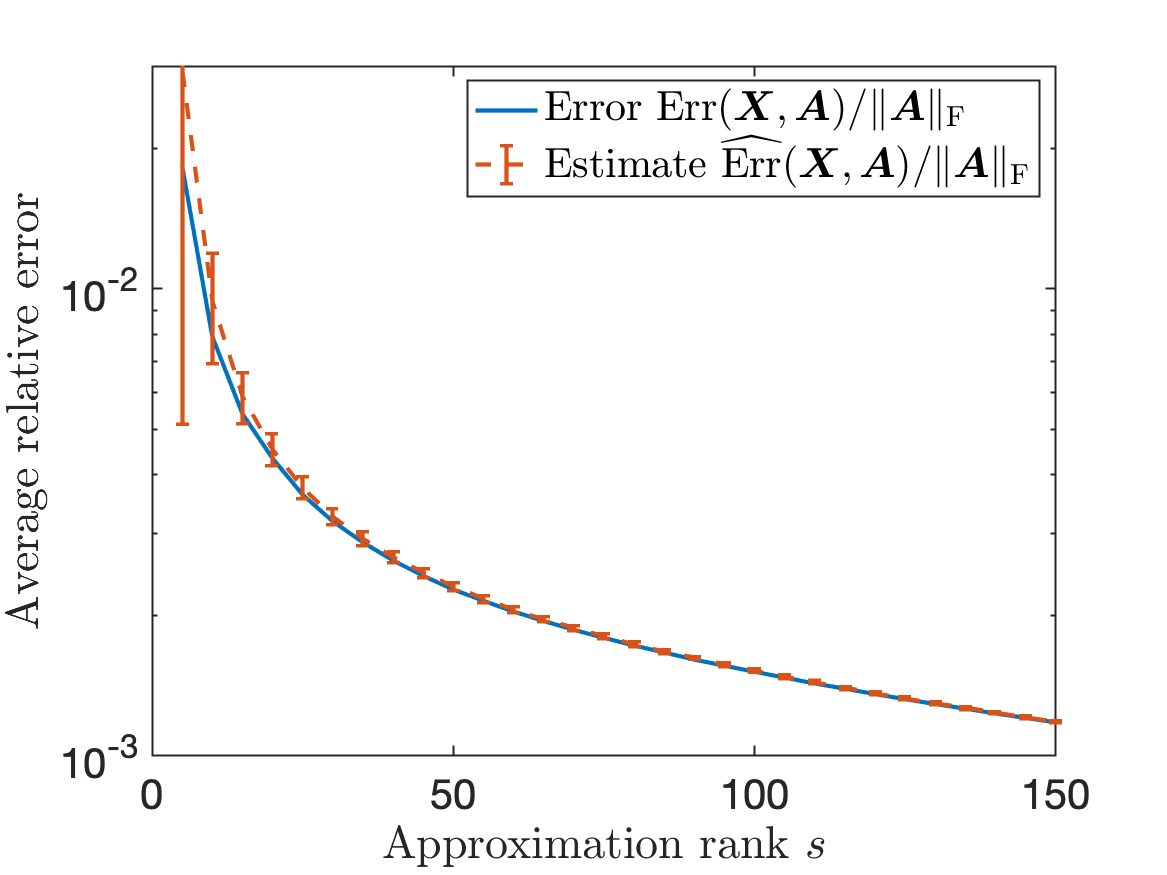
Figure 1: Leave-one-out error estimator. Average relative error $\operatorname{Err}(\boldsymbol{X},\boldsymbol{A})/\left\|\boldsymbol{A}\right\|_{\rm F}$ and normalized error estimate $\widehat{\operatorname{Err}}(\boldsymbol{X},\boldsymbol{A})/\left\|\boldsymbol{A}\right\|_{\rm F}$ for Nyström approximation $\boldsymbol{X}$ to a psd kernel matrix $\boldsymbol{A}\in{}^{10^{4}\times 10^{4}}$. Error and error estimate were computed by an average of $1000$ trials. Error bars show one standard deviation.

1.2 Matrix jackknife motivating example: spectral clustering

Randomized low-rank approximations can also be used for spectral computations (i.e., to approximate eigenvalues, eigenvectors, singular values, etc.). In this case, the low-rank approximation error $\left\|\boldsymbol{A}-\boldsymbol{X}\right\|_{\rm F}$ may only provide indirect information about the accuracy of the computation. For situations such as this, we propose a matrix jackknife variance estimate as a diagnostic tool. In this section, we illustrate the value of this matrix jackknife approach in a spectral clustering application, before introducing the method in generality in Section 3.

1.2.1 Nyström-accelerated spectral clustering

Spectral clustering [29] is an algorithm that uses eigenvectors to assign data points, say $\boldsymbol{c}_{1},\ldots,\boldsymbol{c}_{d}\in{}^{m}$, into groups. To measure similarity between points, we employ a nonnegative, positive definite kernel function $\kappa:{}^{m}\times{}^{m}\to{}_{+}$. One popular choice is the square-exponential kernel

(5) $$\kappa\big{(}\boldsymbol{c},\boldsymbol{c}^{\prime}\big{)}=\exp\left(-\frac{\left\|\boldsymbol{c}-\boldsymbol{c}^{\prime}\right\|^{2}}{2\sigma^{2}}\right).$$

To cluster the data points into groups, we perform the following steps

1. Form the kernel matrix $\boldsymbol{K}$ with entries $k_{ij}=\kappa(\boldsymbol{c}_{i},\boldsymbol{c}_{j})$.

2. Form the diagonal matrix $\boldsymbol{D}=\operatorname{diag}\big{(}\sum_{j=1}^{d}k_{ij}:i=1,\ldots,d\big{)}$.

3. Compute the $n_{\rm dim}$ dominant eigenvectors $\boldsymbol{U}$ of $\boldsymbol{A}\coloneqq\boldsymbol{D}^{-1/2}\boldsymbol{K}\boldsymbol{D}^{-1/2}$.

4. Set $\boldsymbol{W}\coloneqq\boldsymbol{D}^{-1/2}\boldsymbol{U}$.

5. Apply a general-purpose clustering algorithm, such as k-means [1] with $n_{\rm cen}$ centers, to the rows of $\boldsymbol{W}$.

Parameters $n_{\rm dim}$ and $n_{\rm cen}$ set the clustering space dimension and number of clusters.

If one uses direct methods for the eigenvalue problem, the cost of spectral clustering is dominated by the $\mathcal{O}(d^{3})$ cost for the eigenvector calculation in step 3. We can accelerate spectral clustering by using Nyström approximation Eq. 1. The modification is simple: Use the $n_{\rm dim}$ dominant eigenvectors of the Nyström approximation, accessible from the eigendecomposition Eq. 3, in place of the eigenvectors of $\boldsymbol{A}$.

1.2.2 Variance estimation for spectral clustering

As we refine the approximation by increasing $s$, the approximate eigenvectors $\boldsymbol{\widehat{U}}$ will converge to the true eigenvectors $\boldsymbol{U}$ (provided $\boldsymbol{U}$ is unique). But how do we know when we have taken $s$ large enough? Our guiding principle is:

In order to trust the answer provided by a randomized algorithm, the output should be insensitive to the randomness used by the algorithm.

The variance of the matrix output $\boldsymbol{X}$ of a randomized algorithm, defined as

(6) $$\operatorname{Var}(\boldsymbol{X})\coloneqq\operatorname{\mathbb{E}}\left\|\boldsymbol{X}-\operatorname{\mathbb{E}}\boldsymbol{X}\right\|_{\rm F}^{2},$$

provides a quantitative measurement of the sensitivity of the algorithmic output to randomness used by the algorithm. In the context of spectral clustering, we can use a variance estimate to guide our choice of the rank $s$.

To understand the sensitivity of Nyström-accelerated spectral clustering to randomness in the algorithm, we need to specify a target matrix $\boldsymbol{X}$ for variance estimation. The input to k-means clustering are the coordinates

$$\boldsymbol{\widehat{W}}\coloneqq\boldsymbol{D}^{-1/2}\boldsymbol{\widehat{U}}.$$

To respect the invariance of k-means to scaling and rotation of the coordinates, our target for variance estimation will be

$$\boldsymbol{X}=\boldsymbol{\widehat{W}}\boldsymbol{\widehat{W}}^{*}/\big{\|}\boldsymbol{\widehat{W}}\boldsymbol{\widehat{W}}^{*}\big{\|}_{\rm F}.$$

1.2.3 Jackknife variance estimation

Jackknife variance estimation is similar to the leave-one-out error estimator in that we use replicates $\boldsymbol{X}^{(1)},\ldots,\boldsymbol{X}^{(s)}$ recomputed by successively leaving out columns of the random test matrix $\boldsymbol{\Omega}$. As before, we view the target $\boldsymbol{X}$ as a function

$$\boldsymbol{X}=\boldsymbol{X}(\boldsymbol{\Omega})$$

of the test matrix $\boldsymbol{\Omega}$ defining the Nyström approximation by Eq. 1 and Eq. 2. Form jackknife replicates $\boldsymbol{X}^{(j)}$ and their average $\boldsymbol{X}^{(\cdot)}$ via

$$\boldsymbol{X}^{(j)}=\boldsymbol{X}\left(\boldsymbol{\Omega}^{(j)}\right)\quad\text{for $j=1,\ldots,s$}\quad\text{and}\quad\boldsymbol{X}^{(\cdot)}\coloneqq\frac{1}{s}\sum_{j=1}^{s}\boldsymbol{X}^{(j)}$$

where $\boldsymbol{\Omega}^{(j)}$ again denotes $\boldsymbol{\Omega}$ without its $j$th column. The jackknife estimate for $\operatorname{Var}(\boldsymbol{X})$ is

$$\operatorname{Jack}^{2}(\boldsymbol{X})\coloneqq\sum_{j=1}^{s}\left\|\boldsymbol{X}^{(j)}-\boldsymbol{X}^{(\cdot)}\right\|_{\rm F}^{2}.$$

Guarantees for this estimator are provided in Theorem 3.1. Algorithm 3 and LABEL:list:spectral_clustering provide pseudocode and a MATLAB implementation of Nyström-accelerated spectral clustering with the jackknife estimate $\operatorname{Jack}(\boldsymbol{X})$. The cost of forming the jackknife estimate $\operatorname{Jack}(\boldsymbol{X})$ is $\mathcal{O}(s^{2}d)$, much faster than the $\mathcal{O}(qsd^{2})$ cost of Nyström-accelerated spectral clustering.

1.2.4 Numerical example

Correct clustering

Incorrect clustering

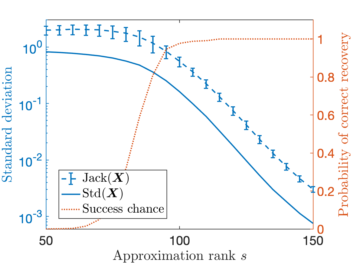
Figure 2: Matrix jackknife for spectral clustering. Top: Example of correct (left) and incorrect (right) clusterings. Bottom: Standard deviation $\operatorname{Std}(\boldsymbol{X})$ and its jackknife estimate $\operatorname{Jack}(\boldsymbol{X})$ (left axis) and success probability of spectral clustering (right axis) versus Nyström approximation rank $50\leq s\leq 150$.

To demonstrate the effectiveness of jackknife variance estimation for spectral clustering, we use the following experimental setup: Consider the task of separating the four letters JACK from a point cloud $\boldsymbol{c}_{1},\ldots,\boldsymbol{c}_{9426}\in{}^{2}$. For spectral clustering, use the square-exponential kernel Eq. 5 and parameters $n_{\rm dim}=n_{\rm cen}=4$. For Nyström, use $q=3$ steps of subspace iteration and test a range of approximation ranks $50\leq s\leq 150$. For each value of $s$, we run $1000$ trials and report the natural Monte Carlo estimate of the standard deviation

(7) $$\operatorname{Std}(\boldsymbol{X})=\left(\operatorname{\mathbb{E}}\left\|\boldsymbol{X}-\operatorname{\mathbb{E}}\boldsymbol{X}\right\|_{\rm F}^{2}\right)^{1/2},$$

the mean and standard deviation for the standard deviation estimate $\operatorname{Jack}(\boldsymbol{X})$, and the empirical success probability for spectral clustering.

Figure 2 shows the results. The estimate $\operatorname{Jack}(\boldsymbol{X})$ overestimates the standard deviation, but by a modest amount (a factor of five at most). The jackknife is not quantitatively sharp, but it is a reliable indicator of whether the variance is high or low.

The jackknife estimate $\operatorname{Jack}(\boldsymbol{X})$ can be used to determine whether the Nyström-based approximations to the eigenvectors are accurate enough for clustering task. At rank $s=50$, clustering is never performed correctly, and the jackknife estimate $\operatorname{Jack}(\boldsymbol{X})\approx 2$ is high. As the approximation rank $s$ is increased, clustering begins to succeed with higher and higher probability and the jackknife estimate $\operatorname{Jack}(\boldsymbol{X})$ decreases, indicating reduced variability. This observation suggests two possible uses for the jackknife estimate:

• User warning. If the jackknife variance estimate is high, provide a warning to the user. This gives the user to determine and fix the problem for themselves by changing the Nyström parameters $s,q$ or the spectral clustering parameters $n_{\rm cen},n_{\rm dim}$.

• Adaptive stopping. Choose parameters $s$ or $q$ for the Nyström approximation adaptively at runtime by increasing these parameters until $\operatorname{Jack}(\boldsymbol{X})$ falls below a tolerance (e.g., $0.1$).

Both of these uses demonstrate the potential for jackknife variance estimation to be helpful in incorporating randomized low-rank approximation into general-purpose software.

1.2.5 Benefits of matrix jackknife variance estimation

The spectral clustering example demonstrates a number of virtues for matrix jackknife variance estimation:

• Flexibility. Matrix jackknife variance estimation can be applied to a very general target function $\boldsymbol{X}(\boldsymbol{\Omega})$ depending on a random test matrix $\boldsymbol{\Omega}$. This allows the jackknife to be applied to a wide array of randomized low-rank approximation algorithms and allows the user to design the variance estimation target for their application.

• Efficiency. By using optimized algorithms (Sections 4 and SM1.2), computation of the jackknife variance estimate can be very fast. For instance, for the clustering problem, the $\mathcal{O}(s^{2}d)$ cost of the jackknife estimate is dwarfed by the $\mathcal{O}(sd^{2})$ cost of the clustering procedure. For $s=150$, computing the jackknife variance estimate amounts to less than 3% of the total runtime.

1.3 Outline

Having introduced our two diagnostics, we present each in more generality; Section 2 discusses leave-one-out error estimation and Section 3 discusses the matrix jackknife. Section 4 discusses efficient computations for both of these diagnostics applied to the randomized SVD and Nyström approximation. Section 5 contains numerical experiments, and Section 6 extends the the matrix jackknife to higher Schatten norms ($p>2$).

1.4 Notation

We work over the field $\mathbb{K}=\real$ or $\mathbb{K}=\mathbb{C}$. Notations ^∗, ^†, and $\left\|\cdot\right\|_{\rm F}$ denote the conjugate transpose, Moore–Penrose pseudoinverse, and Frobenius norm. The expectation of a random variable $X$ is denoted $\operatorname{\mathbb{E}}X$, and its variance is defined as $\operatorname{Var}(X)\coloneqq\operatorname{\mathbb{E}}|X-\operatorname{\mathbb{E}}X|^{2}$. We adopt the convention that nonlinear operators bind before the expectation; for example, $\operatorname{\mathbb{E}}X^{2}\coloneqq\operatorname{\mathbb{E}}(X^{2})$. The variance of a random matrix is given by Eq. 6.

2 Leave-one-out error estimation for low-rank approximation

In this section, we present the leave-one-out error estimation technique introduced in Section 1.1 for more general randomized matrix approximations.

2.1 The estimator

Let $\boldsymbol{A}\in\mathbb{K}^{d_{1}\times d_{2}}$ be a matrix we seek to approximate by a randomized approximation $\boldsymbol{X}$. We are interested in a general class of algorithms which collect information about the matrix $\boldsymbol{A}$ by matrix–vector products

$$\boldsymbol{A}\boldsymbol{\omega}_{1},\ldots,\boldsymbol{A}\boldsymbol{\omega}_{s}$$

with random test vectors $\boldsymbol{\omega}_{1},\ldots,\boldsymbol{\omega}_{s}$. Many algorithms are defined for an arbitrary number of test vectors $s$, allowing us to construct error estimates by leaving out a test vector, resulting in an approximation $\boldsymbol{X}_{s-1}$ defined using only $s-1$ vectors. This motivates the following abstract setup:

• Let $\boldsymbol{\omega}_{1},\ldots,\boldsymbol{\omega}_{s}$ be independent and identically distributed (iid) random vectors in $\mathbb{K}^{d_{2}}$ that are isotropic: $\operatorname{\mathbb{E}}\big{[}\boldsymbol{\omega}_{j}^{\vphantom{*}}\boldsymbol{\omega}_{j}^{*}\big{]}=\mathbf{I}$.

• Let $\boldsymbol{X}$ denote one of two matrix estimators defined for $s$ or $s-1$ inputs:

  $$\boldsymbol{X}:(\mathbb{K}^{d_{2}})^{s}\to\mathbb{K}^{d_{1}\times d_{2}}\quad\textrm{or}\quad\boldsymbol{X}:(\mathbb{K}^{d_{2}})^{s-1}\to\mathbb{K}^{d_{1}\times d_{2}}.$$

• Define estimates $\boldsymbol{X}_{s}\coloneqq\boldsymbol{X}(\boldsymbol{\omega}_{1},\ldots,\boldsymbol{\omega}_{s})$ and $\boldsymbol{X}_{s-1}\coloneqq\boldsymbol{X}(\boldsymbol{\omega}_{1},\ldots,\boldsymbol{\omega}_{s-1})$.

Examples of estimators which fit this description include randomized Nyström approximation, the randomized SVD [11], and randomized block Krylov iteration [17, 26].

We seek to approximate the mean-square error

$$\operatorname{MSE}(\boldsymbol{X}_{s-1},\boldsymbol{A})=\operatorname{\mathbb{E}}\left\|\boldsymbol{A}-\boldsymbol{X}_{s-1}\right\|_{\rm F}^{2}$$

of the $(s-1)$-sample approximation $\boldsymbol{X}_{s-1}$ as a proxy for the mean-square error $\operatorname{MSE}(\boldsymbol{X}_{s})$ of the $s$-sample approximation $\boldsymbol{X}_{s}$. Define the leave-one-out mean-square error estimate

(8) $$\widehat{\operatorname{Err}}^{2}(\boldsymbol{X}_{s-1},\boldsymbol{A})\coloneqq\frac{1}{s}\sum_{j=1}^{s}\left\|\big{(}\boldsymbol{A}-\boldsymbol{X}^{(j)}\big{)}\boldsymbol{\omega}_{j}\right\|^{2},$$

where the replicates $\boldsymbol{X}^{(j)}$ are

$$\boldsymbol{X}^{(j)}=\boldsymbol{X}(\boldsymbol{\omega}_{1},\ldots,\boldsymbol{\omega}_{j-1},\boldsymbol{\omega}_{j+1},\ldots,\boldsymbol{\omega}_{s})\quad\text{for $j=1,\ldots,s$}.$$

This estimator is an unbiased estimator for $\operatorname{MSE}(\boldsymbol{X}_{s-1},\boldsymbol{A})$.

Theorem 2.1 (Leave-one-out error estimator).

With the prevailing notation,

$$\operatorname{MSE}(\boldsymbol{X}_{s-1},\boldsymbol{A})=\operatorname{\mathbb{E}}\,\widehat{\operatorname{Err}}^{2}(\boldsymbol{X}_{s-1},\boldsymbol{A}).$$

Proof 2.2.

For each $j$, $\boldsymbol{X}^{(j)}$ and $\omega_{j}$ are independent. Consequently, letting $\operatorname{\mathbb{E}}_{j}$ denote an expectation over the randomness in $\boldsymbol{\omega}_{j}$ alone, we compute

$$\operatorname{\mathbb{E}}_{j}\big{\|}(\boldsymbol{A}-\boldsymbol{X}^{(j)})\boldsymbol{\omega}_{j}\big{\|}^{2} =\operatorname{\mathbb{E}}_{j}\big{[}\boldsymbol{\omega}_{j}^{*}(\boldsymbol{A}-\boldsymbol{X}^{(j)})^{*}(\boldsymbol{A}-\boldsymbol{X}^{(j)})\boldsymbol{\omega}_{j}^{\vphantom{*}}\big{]}$$

$$=\operatorname{\mathbb{E}}_{j}\operatorname{tr}\big{[}(\boldsymbol{A}-\boldsymbol{X}^{(j)})^{*}(\boldsymbol{A}-\boldsymbol{X}^{(j)})\boldsymbol{\omega}_{j}^{\vphantom{*}}\boldsymbol{\omega}_{j}^{*}\big{]}$$

$$=\operatorname{tr}\big{(}(\boldsymbol{A}-\boldsymbol{X}^{(j)})^{*}(\boldsymbol{A}-\boldsymbol{X}^{(j)})\operatorname{\mathbb{E}}\left[\boldsymbol{\omega}_{j}^{\vphantom{*}}\boldsymbol{\omega}_{j}^{*}\right]\big{)}$$

$$=\operatorname{tr}\big{(}(\boldsymbol{A}-\boldsymbol{X}^{(j)})^{*}(\boldsymbol{A}-\boldsymbol{X}^{(j)})\big{)}=\big{\|}\boldsymbol{A}-\boldsymbol{X}^{(j)}\big{\|}_{\rm F}^{2}.$$

The first line is an identity for the Frobenius norm, the second line is the cyclic property of the trace, the third line is the independence of $\boldsymbol{X}^{(j)}$ and $\boldsymbol{\omega}_{j}$, and the fourth line is the isotropic property of $\boldsymbol{\omega}_{j}$. Thus, by the tower property of conditional expectation, we conclude

$$\operatorname{\mathbb{E}}\,\widehat{\operatorname{Err}}^{2}(\boldsymbol{X}_{s-1},\boldsymbol{A}) =\frac{1}{s}\sum_{j=1}^{s}\operatorname{\mathbb{E}}\,\big{[}\operatorname{\mathbb{E}}_{j}\,\big{\|}\big{(}\boldsymbol{A}-\boldsymbol{X}^{(j)}\big{)}\boldsymbol{\omega}_{j}\big{\|}^{2}\big{]}$$

$$=\frac{1}{s}\sum_{j=1}^{s}\operatorname{\mathbb{E}}\,\big{\|}\big{(}\boldsymbol{A}-\boldsymbol{X}^{(j)}\big{)}\boldsymbol{\omega}_{j}\big{\|}^{2}_{\rm F}=\operatorname{MSE}(\boldsymbol{X}_{s-1},\boldsymbol{A}).$$

This confirms the theorem.

Numerical evidence for the quality of this error estimate is provided in Figs. 1 and 3. With efficient algorithms (Section 4), the leave-one-out error estimator is rapid to compute for the randomized SVD and Nyström approximation.

2.2 Alternatives

Two alternatives to the leave-one-out error estimator are worth mentioning. First, in many situations, it may be possible and computationally cheap to simply compute the error $\left\|\boldsymbol{A}-\boldsymbol{X}\right\|_{\rm F}$ directly. For instance, if $\boldsymbol{X}$ is the approximation produced by the randomized SVD [11], then

$$\left\|\boldsymbol{A}-\boldsymbol{X}\right\|_{\rm F}^{2}=\left\|\boldsymbol{A}\right\|_{\rm F}^{2}-\left\|\boldsymbol{X}\right\|_{\rm F}^{2},$$

which facilitates fast computation of the error if $\boldsymbol{A}$ is a dense or sparse matrix stored in memory. The leave-one-out error estimator should only be used if direct computation of the error is not possible or too expensive. This is the case, for example, in the black-box setting where one has access to $\boldsymbol{A}$ only through the matrix–vector product $\boldsymbol{\omega}\mapsto\boldsymbol{A}\boldsymbol{\omega}$ and adjoint–vector product $\boldsymbol{\omega}\mapsto\boldsymbol{A}^{*}\boldsymbol{\omega}$ operations.

A second alternative is provided by randomized norm estimates [16, §§4–5]. For isotropic random vectors $\boldsymbol{\nu}_{1},\ldots,\boldsymbol{\nu}_{t}$ independent of the random approximation $\boldsymbol{X}$,

(9) $$\frac{1}{t}\sum_{j=1}^{t}\left\|(\boldsymbol{A}-\boldsymbol{X})\boldsymbol{\nu}_{j}\right\|^{2}\quad\text{is an unbiased estimate for}\quad\left\|\boldsymbol{A}-\boldsymbol{X}\right\|_{\rm F}^{2}.$$

The leave-one-out error estimator Eq. 8 has a similar form except that we reuse the test vectors $\boldsymbol{\omega}_{1},\ldots,\boldsymbol{\omega}_{s}$ instead of generating fresh vectors $\boldsymbol{\nu}_{1},\ldots,\boldsymbol{\nu}_{t}$. Because of this reuse, the leave-one-our error estimator is more sample-efficient than the norm estimate Eq. 9. For the leave-one-out error estimator, every matrix–vector product $\boldsymbol{A}\boldsymbol{\omega}_{j}$ is used to both form the approximation $\boldsymbol{X}$ and estimate the error, no extra matrix–vector products required.

3 Matrix jackknife variance estimation

This section outlines our proposal for matrix jackknife variance estimation for more general randomized matrix algorithms. Section 3.1 reviews jackknife variance estimation for scalar quantities. We introduce and analyze the matrix jackknife variance estimator in Section 3.2. Sections 3.3, 3.4, and 3.5 discuss potential applications of the matrix jackknife and complementary topics.

3.1 Tukey’s jackknife variance estimator and the Efron–Stein–Steele inequality

To motivate our matrix jackknife proposal, we begin by presenting the jackknife variance estimator [28] for scalar estimators due to Tukey in Section 3.1.1. In Section 3.1.2, we discuss the Efron–Stein–Steele inequality used in its analysis.

3.1.1 Tukey’s jackknife variance estimator

Consider the problem of estimating the variance of a statistical estimator computed from $s$ random samples. We assume it makes sense to evaluate the estimator with fewer than $s$ samples, as is the case for many classical estimators like the sample mean and variance. This motivates the following setup:

• Let $\omega_{1},\ldots,\omega_{s}$ be independent and identically distributed random elements taking values in a measurable space $\Omega$.

• Let $f$ denote either one of two estimators, defined for $s$ or $s-1$ arguments:

  $$f:\Omega^{s}\to\mathbb{K}\quad\textrm{or}\quad f:\Omega^{s-1}\to\mathbb{K}.$$

• Assume that $f$ is invariant to a reordering of its inputs:

  $$f(\omega_{1},\ldots,\omega_{s})=f(\omega_{\pi(1)},\ldots,\omega_{\pi(s)})\quad\textrm{for any permutation }\pi.$$

• Define estimates $E_{s-1}\coloneqq f(\omega_{1},\ldots,\omega_{s-1})$ and $E_{s}\coloneqq f(\omega_{1},\ldots,\omega_{s})$.

We think of $E_{s}$ as a statistic computed from a collection of samples $\omega_{1},\ldots,\omega_{s}$. We can also evaluate the statistic with only $s-1$ samples, resulting in $E_{s-1}$.

Tukey’s jackknife variance estimator provides an estimate for $\operatorname{Var}(E_{s-1})$, which serves as a proxy for the variance of the $s$-sample estimator $E_{s}$. Define jackknife replicates and mean

$$E^{(j)}\coloneqq f(\omega_{1},\ldots,\omega_{j-1},\omega_{j+1},\ldots,\omega_{s})\quad\mbox{for each }j=1,2,\ldots,s;\quad E^{(\cdot)}\coloneqq\frac{1}{s}\sum_{j=1}^{s}E^{(j)}.$$

The quantities $E^{(1)},\ldots,E^{(s)}$ represent the statistic recomputed with each of the samples $\omega_{1},\ldots,\omega_{s}$ left out in turn.

Tukey’s estimator for $\operatorname{Var}(E_{s-1})$ is given by

(10) $$\widehat{\operatorname{Var}}(E_{s-1})\coloneqq\sum_{j=1}^{s}\left|E^{(j)}-E^{(\cdot)}\right|^{2}.$$

Observe that Tukey’s estimator Eq. 10 is the sample variance of the jackknife replicates $E^{(j)}$ up to a normalizing constant. The form of Tukey’s estimator suggests that the distribution of the jackknife replicates somehow approximates the distribution of the estimator. This intuition can be formalized using the Efron–Stein–Steele inequality.

3.1.2 Efron–Stein–Steele inequality

To analyze Tukey’s estimator, we rely on an inequality of Efron and Stein [7], which was improved by Steele [24]:

Fact 1 (Efron–Stein–Steele inequality).

Let $\omega_{1},\ldots,\omega_{s}\in\Omega$ be independent elements in a measurable space $\Omega$, and let $f:\Omega^{s}\to\mathbb{K}$ be measurable. Let $(\omega_{j}^{\prime}:j=1,\dots,s)$ be an independent copy of $(\omega_{j}:j=1,\dots,s)$. Then

(11) $$\operatorname{Var}\big{(}f\big{(}\omega_{1}^{\vphantom{{}^{\prime}}},\ldots,\omega_{s}^{\vphantom{{}^{\prime}}}\big{)}\big{)}\leq\frac{1}{2}\sum_{i=1}^{s}\operatorname{\mathbb{E}}\Big{|}f\big{(}\omega_{1}^{\vphantom{{}^{\prime}}},\ldots,\omega_{s}^{\vphantom{{}^{\prime}}}\big{)}-f\big{(}\omega_{1}^{\vphantom{{}^{\prime}}},\ldots,\omega_{j-1}^{\vphantom{{}^{\prime}}},\omega_{j}^{\prime},\omega_{j+1}^{\vphantom{{}^{\prime}}},\ldots,\omega_{s}^{\vphantom{{}^{\prime}}}\big{)}\Big{|}^{2}.$$

The complex-valued version of the inequality presented here follows from the more standard version for real values by treating the real and imaginary parts separately.

In the setting of Tukey’s estimator Eq. 10, the samples $\omega_{1},\ldots,\omega_{s-1}$ are identically distributed and the function $f$ depends symmetrically on its arguments. Therefore, the last sample $\omega_{s}$ can be used to fill the role of each $\omega_{j}^{\prime}$ in the right-hand side of Eq. 11. As a consequence, the Efron–Stein–Steele inequality shows that

(12) $$\operatorname{Var}(E_{s-1}) \leq\frac{1}{2}\sum_{i=1}^{s-1}\operatorname{\mathbb{E}}\,\left(E^{(j)}-E^{(s)}\right)^{2}=\frac{1}{2s}\sum_{i,j=1}^{s}\operatorname{\mathbb{E}}\,\left(E^{(i)}-E^{(j)}\right)^{2}$$

$$=\sum_{j=1}^{s}\operatorname{\mathbb{E}}\,\left(E^{(j)}-E^{(\cdot)}\right)^{2}=\operatorname{\mathbb{E}}\,\widehat{\operatorname{Var}}(E_{s-1}).$$

To move from the first line to the second, we expand the square, use the definition of the mean $E^{(\cdot)}=s^{-1}\sum_{j=1}^{s}E^{(j)}$, and regroup terms. This computations shows that Tukey’s variance estimator Eq. 10 overestimates the true variance on average.

3.2 The matrix jackknife estimator of variance

Suppose we are interested in the variance of the output $\boldsymbol{X}\in\mathbb{K}^{d_{1}\times d_{2}}$ to a randomized matrix algorithm. Similar to the scalar setting, we assume that $\boldsymbol{X}$ is a function of independent samples $\omega_{1},\ldots,\omega_{s}$ and that it makes sense to evaluate $\boldsymbol{X}$ with fewer than $s$ samples. The formal setup is as follows:

• Let $\omega_{1},\ldots,\omega_{s}$ be independent and identically distributed random elements in a measurable space $\Omega$.

• Let $\boldsymbol{X}$ denote one of two matrix estimators defined for $s$ or $s-1$ inputs:

  $$\boldsymbol{X}:\Omega^{s}\to\mathbb{K}^{d_{1}\times d_{2}}\quad\textrm{or}\quad\boldsymbol{X}:\Omega^{s-1}\to\mathbb{K}^{d_{1}\times d_{2}}.$$

• Assume $\boldsymbol{X}$ is invariant to reordering of its inputs:

  $$\boldsymbol{X}(\omega_{1},\ldots,\omega_{s})=\boldsymbol{X}(\omega_{\pi(1)},\ldots,\omega_{\pi(s)})\quad\text{for any permutation $\pi$.}$$

• Define estimates $\boldsymbol{X}_{s}\coloneqq\boldsymbol{X}(\omega_{1},\ldots,\omega_{s})$ and $\boldsymbol{X}_{s-1}\coloneqq\boldsymbol{X}(\omega_{1},\ldots,\omega_{s-1})$.

For a randomized low-rank approximation algorithm, the samples $\omega_{1},\ldots,\omega_{s}$ might represent the columns of a test matrix $\boldsymbol{\Omega}$, as they did in Section 1.2.

We are interested in estimating the variance of $\boldsymbol{X}_{s-1}$ as a proxy for the variance of $\boldsymbol{X}_{s}$. We expect that adding additional samples will refine the approximation and thus reduce its variance. Define jackknife replicates $\boldsymbol{X}^{(j)}$ and their average $\boldsymbol{X}^{(\cdot)}$

$$\boldsymbol{X}^{(j)}=\boldsymbol{X}(\omega_{1},\ldots,\omega_{j-1},\omega_{j+1},\ldots,\omega_{s})\quad\mbox{for each }j=1,\ldots,s;\quad\boldsymbol{X}^{(\cdot)}\coloneqq\frac{1}{s}\sum_{j=1}^{s}\boldsymbol{X}^{(j)}.$$

We propose the matrix jackknife estimate

(13) $$\operatorname{Jack}^{2}\big{(}\boldsymbol{X}_{s-1}\big{)}\coloneqq\sum_{j=1}^{s}\left\|\boldsymbol{X}^{(j)}-\boldsymbol{X}^{(\cdot)}\right\|_{\rm F}^{2}$$

for the variance $\operatorname{Var}(\boldsymbol{X}_{s-1})$. The estimator $\operatorname{Jack}(\boldsymbol{X}_{s-1})$ can be efficiently computed for several randomized low-rank approximation, as we shall demonstrate in Section 4. Similar to the classic jackknife variance estimator, we can use the Efron–Stein–Steele inequality to show that this variance estimate is an overestimate on average.

Theorem 3.1 (Matrix jackknife).

With the prevailing notation,

(14) $$\operatorname{Var}(\boldsymbol{X}_{s-1})\leq\operatorname{\mathbb{E}}\,\operatorname{Jack}^{2}\big{(}\boldsymbol{X}_{s-1}\big{)}.$$

Proof 3.2.

Fix a pair of indices $1\leq m\leq d_{1}$ and $1\leq n\leq d_{2}$. Applying Eq. 12 to the $(m,n)$-matrix entry $\left(\boldsymbol{X}_{s-1}\right)_{mn}$, we observe

$$\operatorname{\mathbb{E}}\left|\left(\boldsymbol{X}_{s-1}\right)_{mn}-\operatorname{\mathbb{E}}\left(\boldsymbol{X}_{s-1}\right)_{mn}\right|^{2}\leq\operatorname{\mathbb{E}}\sum_{j=1}^{s}\left|\boldsymbol{X}^{(j)}_{mn}-\boldsymbol{X}^{(\cdot)}_{mn}\right|^{2}$$

Summing this equation over all $1\leq m\leq d_{1}$ and $1\leq n\leq d_{2}$ yields the stated result.

When the jackknife variance estimate is small, Theorem 3.1 shows the variance of the approximation is also small. Empirical evidence (Section 5) suggests that $\operatorname{Var}(\boldsymbol{X}_{s-1})$ and $\operatorname{\mathbb{E}}\,\operatorname{Jack}^{2}(\boldsymbol{X}_{s-1})$ tend to be within an order of magnitude for the algorithms we considered.

It is natural to ask whether we can develop and theoretically jackknife estimates of the bias of randomized matrix algorithms to complement our variance estimate, perhaps using the natural analog of Quenouille’s scalar jackknife bias estimate [20]. This is an interesting question for future work. As we have demonstrated in Section 1.2 and will further demonstrate in Section 5, our variance estimate already provides useful and actionable information for randomized matrix algorithms.

3.3 Uses for matrix jackknife variance estimator

Variance is a useful diagnostic for randomized matrix approximations. When the variance is large, it suggests that one of two issues has arisen:

1. More samples are needed to refine the approximation.

2. The underlying approximation problem is badly conditioned

In either case, the jackknife variance estimate can provide evidence that the computed output should not be trusted.

We anticipate the primary use case for matrix jackknife variance estimation will be for computations using eigenvectors or singular vectors computed by randomized low-rank approximation algorithms such as the randomized SVD and Nyström approximation. Spectral computations with randomized algorithms currently lack effective posterior estimates, making jackknife variance estimation one of the only available tools to assess the quality of the outputs of such computations at runtime. In the context of spectral computations, matrix jackknife variance estimation can be used to adaptively determine the approximation rank $s$ needed to achieve outputs of sufficiently high quality. This was demonstrated in Section 1.2, where we used jackknife variance estimation to determine how large to pick $s$ in a spectral clustering context. As we will later demonstrate in Section 5, we can also use the jackknife variance estimation to detect ill-disposed eigenvectors and to get coordinate-wise variance estimates for singular vector computations.

3.4 Matrix jackknife versus scalar jackknife

Sometimes, we are only interested in scalar outputs of a randomized matrix computation, such as eigenvalues or singular values, entries of eigenvectors or singular vectors, or the trace. In these cases, it might be more efficient to directly apply Tukey’s variance estimator Eq. 10 to assess the variance of these scalars. The matrix jackknife may still be a useful tool because it gives simultaneous variance estimates over many scalar quantities. As examples, the matrix jackknife estimates the maximum variance over all linear functionals:

$$\operatorname{\mathbb{E}}\max_{\left\|\boldsymbol{C}\right\|_{\rm F}\leq 1}\left|\operatorname{tr}(\boldsymbol{C}\boldsymbol{X}_{s-1})-\operatorname{tr}(\boldsymbol{C}\,\operatorname{\mathbb{E}}\boldsymbol{X}_{s-1})\right|^{2}=\operatorname{\mathbb{E}}\left\|\boldsymbol{X}_{s-1}-\operatorname{\mathbb{E}}\boldsymbol{X}_{s-1}\right\|_{\rm F}^{2}\leq\operatorname{\mathbb{E}}\operatorname{Jack}^{2}(\boldsymbol{X}_{s-1}),$$

The matrix jackknife gives the following variance estimate for the singular values:

$$\operatorname{\mathbb{E}}\sum_{j=1}^{\min(d_{1},d_{2})}\left|\sigma_{j}(\boldsymbol{X}_{s-1})-\sigma_{j}(\operatorname{\mathbb{E}}\boldsymbol{X}_{s-1})\right|^{2}=\operatorname{\mathbb{E}}\left\|\boldsymbol{X}_{s-1}-\operatorname{\mathbb{E}}\boldsymbol{X}_{s-1}\right\|_{\rm F}^{2}\leq\operatorname{\mathbb{E}}\operatorname{Jack}^{2}(\boldsymbol{X}_{s-1}).$$

Thus, the matrix jackknife is appealing even when one is interested in multiple scalar-valued functions of the matrix approximation $\boldsymbol{X}_{s-1}$. In addition, efficient algorithms for matrix jackknife variance estimation, as detailed in Section 4, are useful for scalar jackknife variance estimation of functionals of a randomized matrix approximation.

3.5 Related work: bootstrap for randomized matrix algorithms

Bootstrap resampling [6, §5], a close relative of the jackknife, has seen several applications to matrix computations. An early use case was to provide confidence intervals for eigenvalues and eigenvectors of sample covariance matrices [25, §7.2].

A more recent line of work, led by Lopes and collaborators, applies bootstrap resampling to randomized matrix algorithms [13, 14, 15, 32]. The work closest to ours [13] uses the bootstrap to provide asymptotically sharp estimates of the error quantiles with regards to general error metrics for each singular value and singular vector computed by a linear sketched SVD algorithm. In this special case, the bootstrap provides more fine-grained and quantitatively sharp information than the matrix jackknife. Unfortunately, the linear SVD is a poor computational method because its error decays at the Monte Carlo rate.

The main benefit of our matrix jackknife approach is that it applies to very general nonlinear matrix algorithms, such as the randomized SVD and Nyström approximation. These nonlinear algorithms are used far more widely in practice because they produce errors comparable with the best low-rank approximation [11]. The bootstrap is not currently justified in this setting, whereas the jackknife is guaranteed to produce a reliable posterior variance estimate.

4 Case studies in low-rank approximation

In this section, we develop efficient computational procedures to compute the jackknife variance estimate and leave-one-out error estimate for two randomized low-rank approximations, randomized Nyström approximation (Section 4.1) and the randomized SVD (Section 4.2).

4.1 Nyström approximation

Given a test matrix $\boldsymbol{\Omega}\in\mathbb{K}^{d\times s}$, consider again the Nyström approximation Eq. 1 with $q$ steps of subspace iteration Eq. 2 applied to a psd matrix $\boldsymbol{A}\in\mathbb{K}^{d\times d}$:

$$\boldsymbol{X}=\boldsymbol{X}(\boldsymbol{\Omega})\coloneqq\boldsymbol{A}\langle\boldsymbol{\Phi}\rangle=\boldsymbol{A}\boldsymbol{\Phi}(\boldsymbol{\Phi}^{*}\boldsymbol{A}\boldsymbol{\Phi})^{\dagger}(\boldsymbol{A}\boldsymbol{\Phi})^{*}\quad\text{where}\quad\boldsymbol{\Phi}=\boldsymbol{A}^{q}\boldsymbol{\Phi}.$$

The Nyström approximation $\boldsymbol{X}$ is the best psd approximation to $\boldsymbol{A}$ spanned by $\boldsymbol{A}\boldsymbol{\Phi}$ with a psd residual. We focus on the case where $\boldsymbol{\Omega}$ is populated with iid, isotropic columns, such as when $\boldsymbol{\Omega}$ is a standard Gaussian matrix.

We work with the Nyström approximation in eigenvalue decomposition form:

$$\boldsymbol{X}=\boldsymbol{V}\boldsymbol{\Lambda}\boldsymbol{V}^{*}$$

where $\boldsymbol{V}\in\mathbb{K}^{d\times s}$ has orthonormal columns and $\boldsymbol{\Lambda}\in{}^{s\times s}_{+}$ is diagonal. To facilitate efficient computations of our diagnostics, we can compute the Nyström approximation in eigendecomposition form as follows:

1. Draw a test matrix $\boldsymbol{\Omega}\in\mathbb{K}^{d\times s}$ with iid isotropic columns.

2. Apply subspace iteration $\boldsymbol{\Phi}=\boldsymbol{A}^{q}\boldsymbol{\Omega}$.

3. Compute the product $\boldsymbol{Y}=\boldsymbol{A}\boldsymbol{\Omega}$.

4. Orthonormalize $\boldsymbol{Q}=\operatorname{orth}(\boldsymbol{Y})$ using economy QR factorization $\boldsymbol{Y}=\boldsymbol{Q}\boldsymbol{R}$.

5. Compute $\boldsymbol{H}=\boldsymbol{\Omega}^{*}\boldsymbol{Y}$ and Cholesky factorize $\boldsymbol{H}=\boldsymbol{C}^{*}\boldsymbol{C}$.

6. Obtain a singular value decomposition $\boldsymbol{R}\boldsymbol{C}^{-1}=\boldsymbol{U}\boldsymbol{\Sigma}\boldsymbol{Z}^{*}$.

7. Set $\boldsymbol{\Lambda}\coloneqq\boldsymbol{\Sigma}^{2}$ and $\boldsymbol{V}\coloneqq\boldsymbol{Q}\boldsymbol{U}$.

Algorithm 1 provides an implementation with $q=0$ with tricks to improve its numerical stability adapted from [12, 27]. For $q>0$, it may be necessary to introduce additional orthogonalization steps for reasons of numerical stability [23, Alg. 5.2].

Treating the Nyström approximation $\boldsymbol{X}$ as a symmetric function of the iid, isotropic columns $\boldsymbol{\omega}_{1},\ldots,\boldsymbol{\omega}_{s}$ of the test matrix $\boldsymbol{\Omega}$,

$$\boldsymbol{X}=\boldsymbol{X}(\boldsymbol{\omega}_{1},\ldots,\boldsymbol{\omega}_{s}),$$

we can apply both the leave-one-out error estimator and jackknife variance estimation to $\boldsymbol{X}$. Define replicates

$$\boldsymbol{X}^{(j)}=\boldsymbol{X}(\boldsymbol{\omega}_{1},\ldots,\boldsymbol{\omega}_{j-1},\boldsymbol{\omega}_{j+1},\ldots,\boldsymbol{\omega}_{s}).$$

To compute the replicates efficiently, we use the update formula [8, eq. (2.4)]

(15a) $$\boldsymbol{X}^{(j)}=\boldsymbol{V}\left(\boldsymbol{\Lambda}-\boldsymbol{t}_{j}^{\vphantom{*}}\boldsymbol{t}_{j}^{*}\right)\boldsymbol{V}^{*}$$

where $$\boldsymbol{t}_{1},\ldots,\boldsymbol{t}_{s}$$ are the columns of the matrix

(15b) $$\boldsymbol{T}=\boldsymbol{U}^{*}\boldsymbol{R}\boldsymbol{H}^{-1}\cdot\operatorname{diag}\left((\boldsymbol{H}^{-1})_{ii}^{-1/2}:i=1,2,\ldots,s\right).$$

A derivation of this formula is provided in Section A.1.

The update formula facilitates efficient algorithms for the leave-one-out error estimator and jackknife variance estimates for the Nyström approximation and derived quantities like spectral projectors and truncation of $\boldsymbol{X}$ to rank $r<s$. To not belabor the point by presenting all possible variations, Algorithm 1 presents an implementation of Nyström approximation without subspace iteration (i.e., $q=0$) with the leave-one-out error estimate $\widehat{\operatorname{Err}}(\boldsymbol{X},\boldsymbol{A})$. The computation of the error estimate is a simple addition to the algorithm, requiring just a single line and taking only $\mathcal{O}(s^{3})$ operations, independent of the size $d$ of the input matrix. Further variants are discussed in Section SM1.1 and a MATLAB implementation is provided in LABEL:list:nystrom.

Algorithm 1 Nyström approximation ($q=0$) with leave-one-out error estimate

Input: $\boldsymbol{A}\in\mathbb{K}^{d\times d}$ to be approximated and approximation rank $s$
Output: Factors $\boldsymbol{V}\in\mathbb{K}^{d\times s}$ and $\boldsymbol{\Lambda}\in{}^{s\times s}$ defining a rank-$s$ approximation $\boldsymbol{X}=\boldsymbol{V}\boldsymbol{\Lambda}\boldsymbol{V}^{*}$ and leave-one-out error estimate $\widehat{\operatorname{Err}}$

1:$\boldsymbol{\Omega}\leftarrow\mathtt{randn}(d,s)$

2:$\boldsymbol{Y}\leftarrow\boldsymbol{A}\boldsymbol{\Omega}$

3:$\nu\leftarrow\epsilon_{\rm mach}\left\|\boldsymbol{Y}\right\|$ and $\boldsymbol{Y}\leftarrow\boldsymbol{Y}+\nu\boldsymbol{\Omega}$ $\triangleright$ Shift for numerical stability

4:$(\boldsymbol{Q},\boldsymbol{R})\leftarrow\mathtt{qr}(\boldsymbol{Y},\texttt{'econ'})$ $\triangleright$ Economy QR Factorization

5:$\boldsymbol{H}\leftarrow\boldsymbol{\Omega}^{*}\boldsymbol{Y}$

6:$\boldsymbol{C}\leftarrow\mathtt{chol}((\boldsymbol{H}+\boldsymbol{H}^{*})/2)$ $\triangleright$ Upper triangular Cholesky decomposition $\boldsymbol{H}=\boldsymbol{C}^{*}\boldsymbol{C}$

7:$(\boldsymbol{U},\boldsymbol{\Sigma},\sim)\leftarrow\mathtt{svd}(\boldsymbol{R}\boldsymbol{C}^{-1})$ $\triangleright$ Triangular solve

8:$\boldsymbol{\Lambda}\leftarrow\max(\boldsymbol{\Sigma}^{2}-\nu\mathbf{I},0)$ $\triangleright$ Entrywise maximum, shift back for numerical stability

9:$\boldsymbol{V}\leftarrow\boldsymbol{Q}\boldsymbol{U}$

10:$\widehat{\operatorname{Err}}\leftarrow\left\|(\boldsymbol{R}\boldsymbol{C}^{-1})\boldsymbol{C}^{-*}\cdot\operatorname{diag}\{(\boldsymbol{H}^{-1}_{ii})^{-1}:i=1,\ldots,s)\}\right\|_{\rm F}/\sqrt{s}$

4.2 Randomized SVD

The randomized SVD computes a rank-$s$ approximation to $\boldsymbol{A}\in\mathbb{K}^{d_{1}\times d_{2}}$ formed as an economy SVD $\boldsymbol{X}=\boldsymbol{U}\boldsymbol{\Sigma}\boldsymbol{V}^{*}$, where $\boldsymbol{U}\in\mathbb{K}^{d_{1}\times s}$ and $\boldsymbol{V}\in\mathbb{K}^{d_{2}\times s}$ have orthonormal columns and $\boldsymbol{\Sigma}\in{}^{s\times s}_{+}$ is diagonal. With $q\geq 0$ steps of subspace iteration, the algorithm proceeds as follows:

1. Draw a test matrix $\boldsymbol{\Omega}\in\mathbb{K}^{d_{2}\times s}$ with iid isotropic columns.

2. Compute the product $\boldsymbol{Y}=(\boldsymbol{A}\boldsymbol{A}^{*})^{q}\boldsymbol{A}\boldsymbol{\Omega}$.

3. Orthonormalize $\boldsymbol{Q}=\operatorname{orth}(\boldsymbol{Y})$ using economy QR factorization $\boldsymbol{Y}=\boldsymbol{Q}\boldsymbol{R}$.

4. Form the matrix $\boldsymbol{C}=\boldsymbol{Q}^{*}\boldsymbol{A}$.

5. Compute an economy SVD $\boldsymbol{C}=\boldsymbol{W}\boldsymbol{\Sigma}\boldsymbol{V}^{*}$.

6. Set $\boldsymbol{U}=\boldsymbol{Q}\boldsymbol{W}$.

The output $\boldsymbol{X}$ is a symmetric function of the iid, isotropic columns $\boldsymbol{\omega}_{1},\ldots,\boldsymbol{\omega}_{s}$ of $\boldsymbol{\Omega}$,

$$\boldsymbol{X}=\boldsymbol{X}(\boldsymbol{\omega}_{1},\ldots,\boldsymbol{\omega}_{s}),$$

making it a candidate for leave-one-out error estimation and jackknife variance estimation.

To compute the replicates efficiently, we will use the following update formula for the $\boldsymbol{Q}$ matrix in the randomized SVD [8, eq. (2.1)]:

(16) $$\boldsymbol{Q}^{(j)}\left(\boldsymbol{Q}^{(j)}\right)^{*}=\boldsymbol{Q}\left(\mathbf{I}-\boldsymbol{t}_{j}^{\vphantom{*}}\boldsymbol{t}_{j}^{*}\right)\boldsymbol{Q}^{*}$$

where $\boldsymbol{Q}^{(j)}$ denotes the $\boldsymbol{Q}$ matrix produced by the randomized SVD algorithm executed without the $j$th column of $\boldsymbol{\Omega}$ and the vectors $\boldsymbol{t}_{1},\ldots,\boldsymbol{t}_{s}$ are the normalized columns of $(\boldsymbol{R}^{*})^{-1}$. With this formula, the replicates are easily computed

(17) $$\boldsymbol{X}^{(j)}=\boldsymbol{Q}^{(j)}\left(\boldsymbol{Q}^{(j)}\right)^{*}\boldsymbol{A}=\boldsymbol{Q}\left(\mathbf{I}-\boldsymbol{t}_{j}^{\vphantom{*}}\boldsymbol{t}_{j}^{*}\right)\boldsymbol{Q}^{*}\boldsymbol{A}=\boldsymbol{U}(\mathbf{I}-\boldsymbol{W}^{*}\boldsymbol{t}_{j}^{\vphantom{*}}\boldsymbol{t}_{j}^{*}\boldsymbol{W})\boldsymbol{\Sigma}\boldsymbol{V}^{*}.$$

The update formula enables efficient algorithms for the leave-one-out error estimator and jackknife variance estimator for the approximation $\boldsymbol{X}$ and derived quantities like projectors onto singular subspaces and truncation of $\boldsymbol{X}$ to rank $r<s$. As one example, Algorithm 2 gives an implementation the randomized SVD with no subspace iteration ($q=0$) with the leave-one-out error estimator $\widehat{\operatorname{Err}}(\boldsymbol{X},\boldsymbol{A})$. The leave-one-out error estimator requires just two lines and runs in $\mathcal{O}(s^{3})$ operations. Further variants are discussed in Section SM1.3 and a MATLAB implementation is provided in LABEL:list:randsvd.

Algorithm 2 Randomized SVD ($q=0$) with jackknife variance estimate

Input: $\boldsymbol{A}\in\mathbb{K}^{d_{1}\times d_{2}}$ to be approximated and approximation rank $s$
Output: Factors $\boldsymbol{U}\in\mathbb{K}^{d_{1}\times s}$, $\boldsymbol{\Sigma}\in{}^{s\times s}$, and $\boldsymbol{V}\in\mathbb{K}^{d_{2}\times s}$ defining a rank-$s$ approximation $\boldsymbol{X}=\boldsymbol{U}\boldsymbol{\Sigma}\boldsymbol{V}^{*}$, leave-one-out error estimate $\widehat{\operatorname{Err}}=\widehat{\operatorname{Err}}(\boldsymbol{X},\boldsymbol{A})$

1:$\boldsymbol{\Omega}\leftarrow\mathtt{randn}(d_{2},s)$

2:$\boldsymbol{Y}\leftarrow\boldsymbol{A}\boldsymbol{\Omega}$

3:$(\boldsymbol{Q},\boldsymbol{R})\leftarrow\mathtt{qr}(\boldsymbol{Y},\texttt{'econ'})$ $\triangleright$ Economy QR Factorization

4:$\boldsymbol{C}\leftarrow\boldsymbol{Q}^{*}\boldsymbol{A}$

5:$(\boldsymbol{W},\boldsymbol{\Sigma},\boldsymbol{V})\leftarrow\mathtt{svd}(\boldsymbol{C},\texttt{'econ'})$

6:$\boldsymbol{U}\leftarrow\boldsymbol{Q}\boldsymbol{W}$

7:$\boldsymbol{G}\leftarrow(\boldsymbol{R}^{*})^{-1}$

8:$\widehat{\operatorname{Err}}\leftarrow\left(s^{-1}\sum_{j=1}^{s}\left\|\boldsymbol{G}(:,j)\right\|^{-2}\right)^{1/2}$

5 Numerical experiments

In this section, we showcase numerical examples that demonstrate the effectiveness of the matrix jackknife variance estimate and leave-one-our error estimate for the Nyström approximation and randomized SVD. All numerical experiments work over the real numbers, $\mathbb{K}=\real$.

5.1 Experimental setup

To evaluate our diagnostics for matrices with different spectral characteristics, we consider synthetic test matrices from [27, §5]:

(NoisyLR) $$\boldsymbol{A} =\operatorname{diag}(\underbrace{1,\ldots,1}_{R\textrm{ times}},0\ldots,0)+\xi d^{-1}\boldsymbol{G}\boldsymbol{G}^{*}\in{}^{d\times d}.$$

(ExpDecay) $$\boldsymbol{A} =\operatorname{diag}(\underbrace{1,\ldots,1}_{R\textrm{ times}},10^{-q},10^{-2q},\ldots,10^{-(d-R)q})\in{}^{d\times d}.$$

Here, $\xi,q\in\real$ are parameters, and $\boldsymbol{G}\in{}^{d\times d}$ is a standard Gaussian matrix. Using diagonal test matrices is justified by the observation that the randomized SVD, Nyström approximation, and our diagnostics are orthogonally invariant when $\boldsymbol{\Omega}$ is a standard Gaussian matrix, which we use. We also consider matrices from applications:

• Velocity. We consider a matrix $\boldsymbol{A}\in{}^{25096\times 1000}$ whose columns are snapshots of the velocity and pressure from simulations of a fluid flow past a cylinder. We thank Beverley McKeon and Sean Symon for this data.

• Spectral clustering. The matrix $\boldsymbol{A}$ matrix from the spectral clustering example Section 1.2.4.

We apply the jackknife variance estimate and leave-one-out error estimate to the randomized Nyström approximation and randomized SVD with a standard Gaussian test matrix $\boldsymbol{\Omega}$ for a range of values for the approximation rank $s$. For each value of $s$, we estimate the mean error $\operatorname{Err}$ Eq. 4, standard deviation $\operatorname{Std}$ Eq. 7, mean jackknife estimate $\operatorname{Jack}$, or mean leave-one-our error estimator $\widehat{\operatorname{Err}}$ using $1000$ independent trials. Error bars on all figures show one standard deviation.

5.2 Leave-one-out error estimator for randomized SVD

First, we apply leave-one-out error estimation to estimate the error for the randomized SVD

(18) $$\boldsymbol{X}=\boldsymbol{U}\boldsymbol{\Sigma}\boldsymbol{V}^{*}.$$

We set $q=0$. Figure 3 shows the results for three examples in the previous section. In all cases, error estimate $\widehat{\operatorname{Err}}(\boldsymbol{X},\boldsymbol{A})$ tracks the true error $\operatorname{Err}(\boldsymbol{X},\boldsymbol{A})$ closely. Additional examples and analogous plots for randomized Nyström approximation are provided in Appendix SM2.

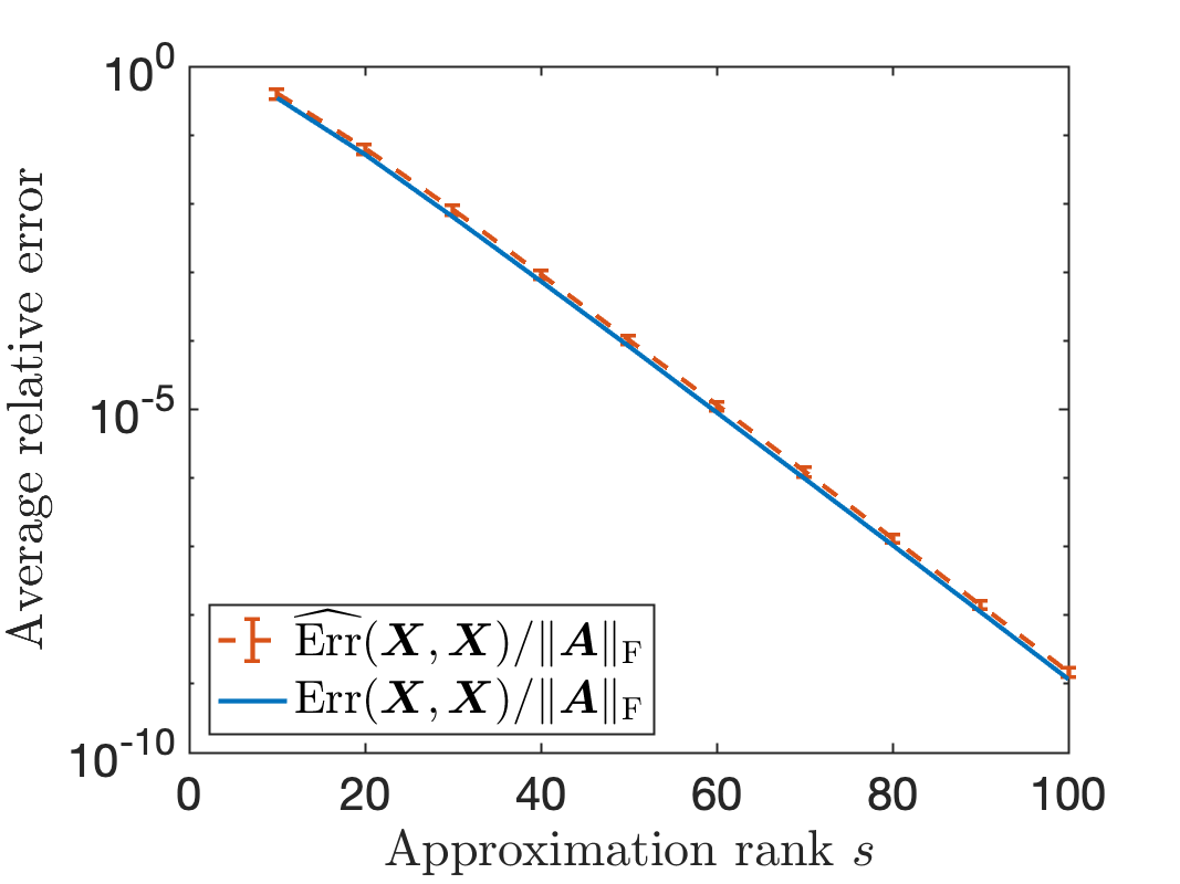
ExpDecay$(q\!=\!0.1,R\!=\!5)$

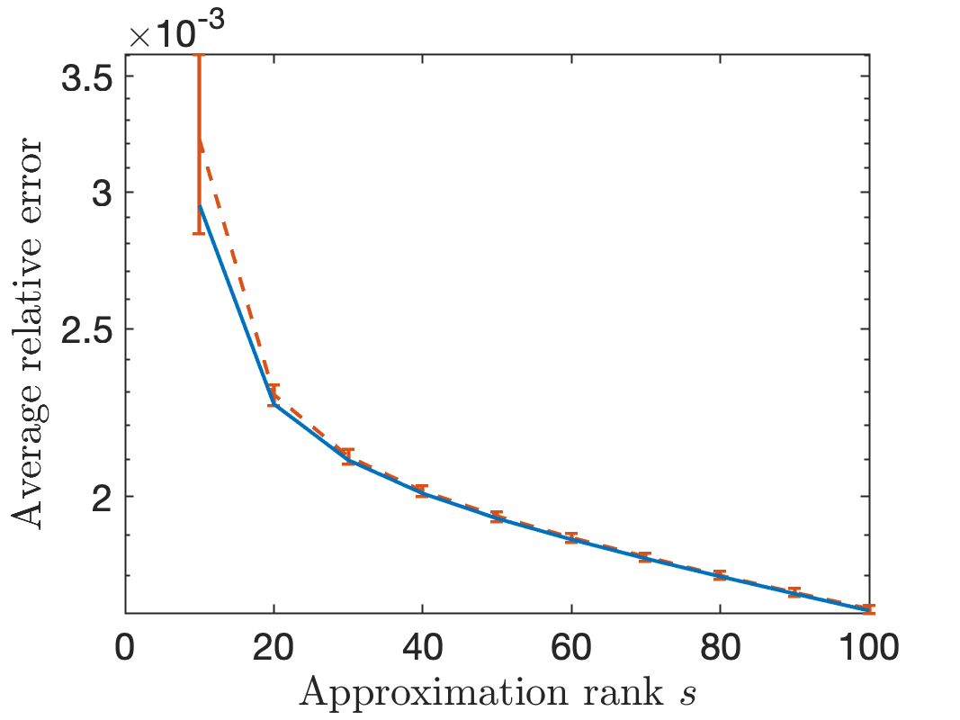
NoisyLR$(\xi\!=\!10^{-4},R\!=\!5)$

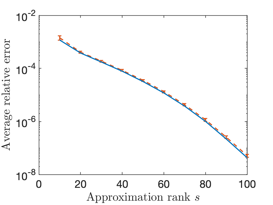
Velocity

Figure 3: Leave-one-out error estimator for randomized SVD. Error and error estimate for randomized SVD ($q=0$) approximation for three different matrices.

5.3 Matrix jackknife for projectors onto singular subspaces

Consider the task of computing the projector $\boldsymbol{\Pi}$ onto the dominant $5$-dimensional right singular subspace to a matrix $\boldsymbol{A}$. The randomized SVD $\boldsymbol{A}\approx\boldsymbol{U}\boldsymbol{\Sigma}\boldsymbol{V}^{*}$ yields the approximation

(19) $$\boldsymbol{X}=\boldsymbol{V}(:,1:5)\boldsymbol{V}(:,1:5)^{*}.$$

Figure 4 shows the mean error $\operatorname{Err}(\boldsymbol{X},\boldsymbol{\Pi})$, standard deviation $\operatorname{Std}(\boldsymbol{X})$, and the jackknife estimate $\operatorname{Jack}(\boldsymbol{X})$ for the same three test matrices as previous. We again set $q=0$. Consistent with Theorem 3.1, the jackknife estimate $\operatorname{Jack}(\boldsymbol{X})$ is an overestimate of $\operatorname{Std}(\boldsymbol{X})$ by a factor of $2\times$ to $8\times$. While the jackknife is not quantitatively sharp, it provides an order of magnitude estimate of the standard deviation and is a useful diagnostic for the quality of the computed output. Additional examples and plots for randomized Nyström approximations of projectors onto invariant subspaces are provided in Appendix SM2.

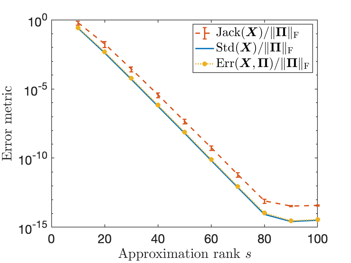
ExpDecay$(q\!=\!0.1,R\!=\!5)$

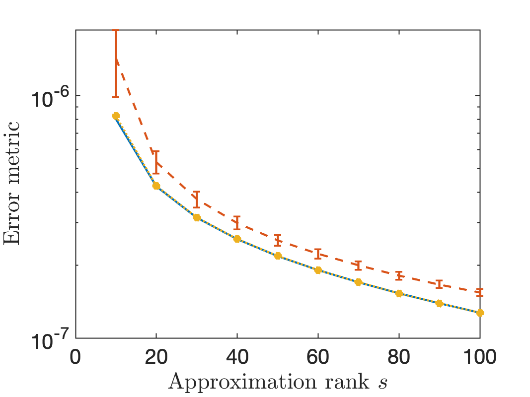
NoisyLR$(\xi\!=\!10^{-4},R\!=\!5)$

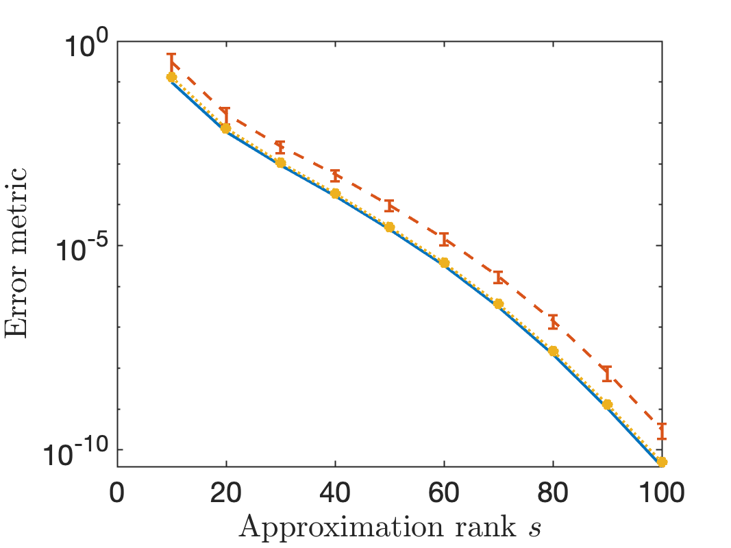
Velocity

Figure 4: Matrix jackknife for projectors onto singular subspaces. Error, standard deviation, and jackknife estimate for randomized SVD ($q=0$) approximation $\boldsymbol{X}$ Eq. 19 to the projector $\boldsymbol{\Pi}$ onto the span of the five dominant right singular vectors for three different matrices.

5.4 Application: Diagnosing ill-conditioning for spectral clustering

Jackknife variance estimates can be used to identify situations when a computational task is ill-posed or ill-conditioned. In such cases, refining the approximation (i.e., increasing $s$ or $q$) may be of little help to improve the quality of the computation.

As an example, consider the spectral clustering application from Section 1.2. In Nyström-accelerated spectral clustering, we use the dominant $n_{\rm dim}$ eigenvectors of a Nyström approximation $\boldsymbol{V}\boldsymbol{\Lambda}\boldsymbol{V}^{*}$ as coordinates for k-means clustering. For spectral clustering to be reliable, we should pick the parameter $n_{\rm dim}$ such that these coordinates are well-conditioned; that is, they should not be highly sensitive to small changes in the normalized kernel matrix $\boldsymbol{A}$. For the example in Section 1.2.4, the five largest eigenvalues of $\boldsymbol{A}$ are

$$\lambda_{1} =0.999999999999999$$

$$\lambda_{2} =0.999999998639842$$

$$\lambda_{3} =0.999999940523446$$

$$\lambda_{4} =0.999999931126177$$

$$\lambda_{5} =0.99\mathbf{7}867975285136$$

The first four eigenvalues agree up to eight digits of accuracy, with the fifth eigenvalue separated by $\lambda_{4}-\lambda_{5}\approx 2\times 10^{-3}$. Based on these values, the natural parameter setting would be $n_{\rm dim}=4$, as the first four eigenvalues are nearly indistinguishable but are well-separated from the fifth.

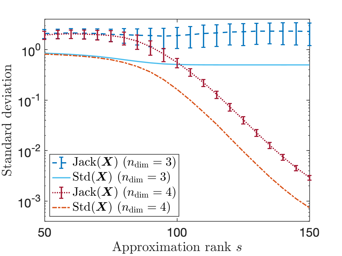
Figure 5: Detecting ill-conditioning. Standard deviation and jackknife estimate for the Nyström spectral projector Eq. 20 associated with the dominant $n_{\rm dim}$-dimensional invariant subspace for $n_{\rm dim}\in\{3,4\}$ for the spectral clustering matrix.

When we use Nyström-accelerated spectral clustering, we do not have access to the true eigenvalues of the matrix $\boldsymbol{A}$ and thus can have difficulties selecting the parameter $n_{\rm dim}$ appropriately. Fortunately, the jackknife variance estimate can help warn the user of a poor choice for $n_{\rm dim}$. Let

(20) $$\boldsymbol{X}=\boldsymbol{V}(:,1:n_{\rm dim})\boldsymbol{V}(:,1:n_{\rm dim})^{*}$$

be the orthoprojector onto the dominant $n_{\rm dim}$-dimensional invariant subspace of the Nyström approximation $\boldsymbol{V}\boldsymbol{\Lambda}\boldsymbol{V}^{*}$. Figure 5 shows the standard deviation $\operatorname{Std}(\boldsymbol{X})$ and its jackknife estimate $\operatorname{Jack}(\boldsymbol{X})$ for both $n_{\rm dim}=3$ and $n_{\rm dim}=4$. As in Section 1.2.4, use $q=3$ and $50\leq s\leq 150$. For the good parameter setting $n_{\rm dim}=4$, the variance decreases sharply as $s$ is increased. For the bad choice $n_{\rm dim}=3$, the variance remains persistently high, even as the approximation is refined. This provides evidence to the user that $\boldsymbol{X}$ is poorly conditioned and allows the user to fix this by changing the parameter $n_{\rm dim}$.

5.5 Application: POD modes

(a) Exact

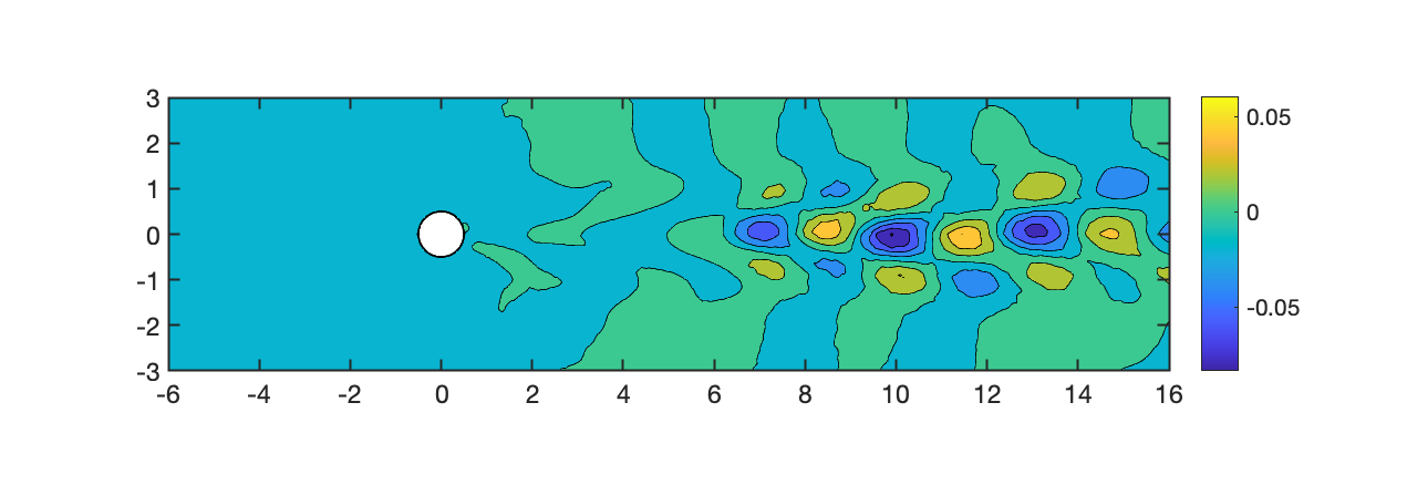
(b) Randomized SVD ($s=20$, $q=0$)

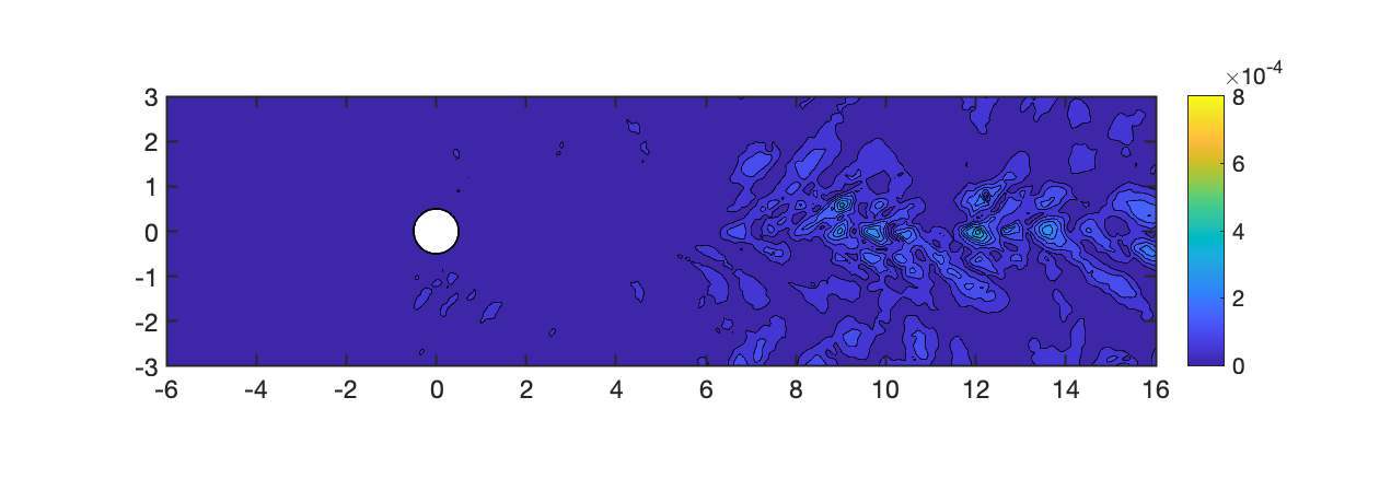
(c) Error

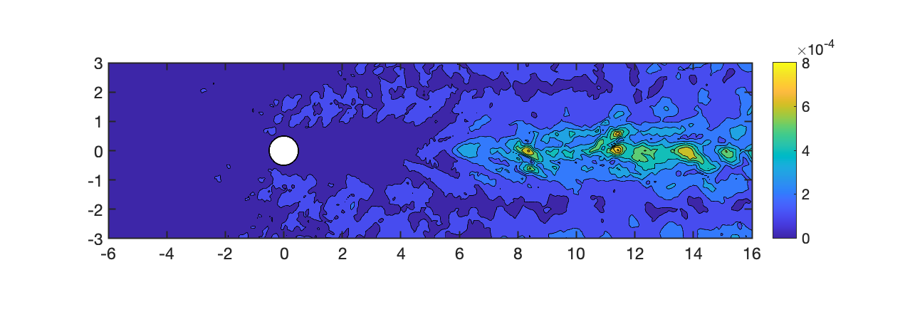
(d) Jackknife standard deviation estimate

Figure 6: Jackknife for singular vector. These panels assess the entrywise errors in the streamwise velocity from the fifth left singular vector of the velocity test matrix. Panel (6(a)) shows the exact answer, and panel (6(b)) shows the estimate produced by the randomized SVD. Panels (6(c)) and (6(d)) display the error and the the Tukey jacknife standard deviation estimate. The jackknife estimate presents a descriptive portrait of where the error is localized.

Jackknife variance estimation can be used to give more fine-grained information about a randomized matrix computation. In Fig. 6, we compute a (scalar) jackknife variance estimate for the absolute value of each entry of the fifth left singular vector of the velocity matrix computed using the randomized SVD with $s=20$ and $q=0$. (The absolute value is introduced to avoid sign ambiguities.)

Left singular vectors of a matrix of simulation data are known as POD modes and are useful for data visualization and model reduction. Since variance is a lower bound on the mean-square error, the coordinate-wise jackknife variance estimates can be used a diagnostic to help identify regions of a POD mode that have high error. This is demonstrated in Fig. 6; the jackknife estimate is not quantitatively sharp but paints a descriptive portrait of where the errors are localized.

6 Extension: Variance estimates for higher Schatten norms

The variance estimate $\operatorname{Jack}(\boldsymbol{X})$ serves as an estimate for the Frobenius-norm variance

$$\operatorname{Jack}^{2}(\boldsymbol{X})\approx\operatorname{Var}(\boldsymbol{X})=\operatorname{\mathbb{E}}\left\|\boldsymbol{X}-\operatorname{\mathbb{E}}\boldsymbol{X}\right\|^{2}_{\rm F}.$$

Often, it is more desirable to have error or variance estimates for Schatten norms ${\left|\kern-1.07639pt\left|\kern-1.07639pt\left|\cdot\right|\kern-1.07639pt\right|\kern-1.07639pt\right|}_{p}$ with $p>2$, defined as the $\ell_{p}$ norm of the singular values:

$${\left|\kern-1.07639pt\left|\kern-1.07639pt\left|\boldsymbol{B}\right|\kern-1.07639pt\right|\kern-1.07639pt\right|}_{p}^{p}\coloneqq\sum_{j=1}^{\min(d_{1},d_{2})}\sigma_{j}^{p}(\boldsymbol{B}).$$

One can also construct jackknife estimates for the variance in higher Schatten norms, although the estimates take more intricate forms. For this section, fix an even number $p\geq 2$ and assume the same setup as Section 3.2 with the additional stipulation that the samples $\omega_{1},\ldots,\omega_{s}$ take values in a Polish space $\Omega$.

The jackknife variance estimate is defined as follows. Consider matrix-valued jackknife variance proxies:

$$\boldsymbol{\widehat{\operatorname{Var}}}_{1}(\boldsymbol{X}_{s-1})\coloneqq\frac{1}{2}\sum_{j=1}^{s-1}\left|\boldsymbol{X}^{(s)}-\boldsymbol{X}^{(j)}\right|^{2}\quad\textrm{and}\quad\boldsymbol{\widehat{\operatorname{Var}}}_{2}(\boldsymbol{X}_{s-1})\coloneqq\frac{1}{2}\sum_{j=1}^{s-1}\left|\boldsymbol{X}^{(s)}-\boldsymbol{X}^{(j)}\right|_{*}^{2}.$$

Define the Schatten $p$-norm variance estimate

$$\operatorname{Jack}_{p}(\boldsymbol{X}_{s-1})\coloneqq 2^{-\tfrac{1}{p}}\sqrt{2(p-1)}\left({\left|\kern-1.07639pt\left|\kern-1.07639pt\left|\boldsymbol{\widehat{\operatorname{Var}}}_{1}\right|\kern-1.07639pt\right|\kern-1.07639pt\right|}_{p/2}^{p/2}+{\left|\kern-1.07639pt\left|\kern-1.07639pt\left|\boldsymbol{\widehat{\operatorname{Var}}}_{2}\right|\kern-1.07639pt\right|\kern-1.07639pt\right|}_{p/2}^{p/2}\right)^{1/p}.$$

This quantity seeks to approximate

$$\operatorname{Jack}_{p}^{p}(\boldsymbol{X}_{s-1})\approx\operatorname{\mathbb{E}}{\left|\kern-1.07639pt\left|\kern-1.07639pt\left|\boldsymbol{X}_{s-1}-\operatorname{\mathbb{E}}\boldsymbol{X}_{s-1}\right|\kern-1.07639pt\right|\kern-1.07639pt\right|}_{p}^{p}.$$

A matrix generalization of the Efron–Stein–Steele inequality [18, Thm. 4.2] shows this jackknife variance estimate overestimates the Schatten $p$-norm variance in the sense

$$\operatorname{\mathbb{E}}{\left|\kern-1.07639pt\left|\kern-1.07639pt\left|\boldsymbol{X}_{s-1}-\operatorname{\mathbb{E}}\boldsymbol{X}_{s-1}\right|\kern-1.07639pt\right|\kern-1.07639pt\right|}_{p}^{p}\leq\operatorname{\mathbb{E}}\,\operatorname{Jack}_{p}^{p}(\boldsymbol{X}_{s-1}).$$

The techniques we introduce in Section 4 can be extended in a natural way to compute $\operatorname{Jack}_{p}(\boldsymbol{X}_{s-1})$ efficiently for the randomized SVD and Nyström approximation.

Appendix A Derivation of update formulas

In this section, we provide proofs of the update formulas Eq. 15 and Eq. 16.

A.1 Proof of Eq. 15

Assume without loss of generality that $j=s$, instate the notation of Section 4.1, and assume $\boldsymbol{H}$ is invertible. The key ingredient is the following consequence of the Banachiewicz inversion formula [19, eq. (0.7.2)]:

$$\begin{bmatrix}\big{(}\boldsymbol{H}^{(s)}\big{)}^{-1}&\boldsymbol{0}\\ \boldsymbol{0}^{*}&0\end{bmatrix}=\boldsymbol{H}^{-1}-\frac{\boldsymbol{H}^{-1}\mathbf{e}_{s}^{\vphantom{*}}\mathbf{e}_{s}^{*}\boldsymbol{H}^{-1}}{\mathbf{e}_{s}^{*}\boldsymbol{H}^{-1}\mathbf{e}_{s}^{\vphantom{*}}}.$$

Using this formula and letting $\boldsymbol{R}_{-s}$ denote $\boldsymbol{R}$ without its $s$th column, we compute

$$\boldsymbol{X}^{(s)}=\boldsymbol{Q}\boldsymbol{R}_{-s}^{\vphantom{*}}\big{(}\boldsymbol{H}^{(s)}\big{)}^{-1}\boldsymbol{R}_{-s}^{*}\boldsymbol{Q}^{*}=\boldsymbol{X}-\frac{\boldsymbol{Q}\boldsymbol{R}\boldsymbol{H}^{-1}\mathbf{e}_{s}^{\vphantom{*}}\mathbf{e}_{s}^{*}\boldsymbol{H}^{-1}\boldsymbol{R}^{*}\boldsymbol{Q}^{*}}{\mathbf{e}_{s}^{*}\boldsymbol{H}^{-1}\mathbf{e}_{s}^{\vphantom{*}}}.$$

Since $\boldsymbol{Q}=\boldsymbol{V}\boldsymbol{U}^{*}$ and $\boldsymbol{X}=\boldsymbol{V}\boldsymbol{\Lambda}\boldsymbol{V}^{*}$, we thus have

$$\boldsymbol{X}^{(s)}=\boldsymbol{V}\left(\boldsymbol{\Lambda}-\frac{\boldsymbol{U}^{*}\boldsymbol{R}\boldsymbol{H}^{-1}\mathbf{e}_{s}^{\vphantom{*}}\mathbf{e}_{s}^{*}\boldsymbol{H}^{-1}\boldsymbol{R}^{*}\boldsymbol{Q}^{*}\boldsymbol{U}}{\mathbf{e}_{s}^{*}\boldsymbol{H}^{-1}\mathbf{e}_{s}^{\vphantom{*}}}\right)\boldsymbol{V}^{*}=\boldsymbol{V}\left(\boldsymbol{\Lambda}-\boldsymbol{t}_{s}^{\vphantom{*}}\boldsymbol{t}_{s}^{*}\right)\boldsymbol{V}^{*},$$

where $\boldsymbol{t}_{s}$ is defined in Eq. 15b. The formula is established. $\proofbox$

A.2 Proof of Eq. 16

Fix $j\in\{1,\ldots,s\}$, instate the notation of Section 4.2, and assume $\boldsymbol{R}$ is invertible. First observe that

$$\boldsymbol{Y}^{(j)}=\boldsymbol{Q}\boldsymbol{R}_{-j},$$

where $\boldsymbol{R}_{-j}$ is $\boldsymbol{R}$ without its $j$th column. To compute $\boldsymbol{Q}^{(j)}$, we need an economy QR factorization of $\boldsymbol{Y}^{(j)}=\boldsymbol{Q}\boldsymbol{R}_{-j}$. To this end, compute a (full) QR decomposition of $\boldsymbol{R}_{-j}$:

(21) $$\boldsymbol{R}_{-j}=\begin{bmatrix}\boldsymbol{Q}^{\prime}&\boldsymbol{t}_{j}\end{bmatrix}\begin{bmatrix}\boldsymbol{R}^{(j)}\\ \boldsymbol{0}^{*}\end{bmatrix},$$

where $\boldsymbol{Q}^{\prime}\in\mathbb{K}^{s\times(s-1)}$, $\boldsymbol{R}^{(j)}\in\mathbb{K}^{(s-1)\times(s-1)}$, and $\boldsymbol{t}_{j}\in\mathbb{K}^{s}$. Then

$$\boldsymbol{Y}^{(j)}=\boldsymbol{Q}^{(j)}\boldsymbol{R}^{(j)}\quad\text{for}\quad\boldsymbol{Q}^{(j)}=\boldsymbol{Q}\boldsymbol{Q}^{\prime}$$

is an economy QR decomposition of $\boldsymbol{Y}^{(j)}$. Since $\begin{bmatrix}\boldsymbol{Q}^{\prime}&\boldsymbol{t}_{j}\end{bmatrix}$ is orthogonal, we have

$$\mathbf{I}=\begin{bmatrix}\boldsymbol{Q}^{\prime}&\boldsymbol{t}_{j}\end{bmatrix}\begin{bmatrix}\boldsymbol{Q}^{\prime}&\boldsymbol{t}_{j}\end{bmatrix}^{*}=\boldsymbol{Q}^{\prime}(\boldsymbol{Q}^{\prime})^{*}+\boldsymbol{t}_{j}^{\vphantom{*}}\boldsymbol{t}_{j}^{*}\implies\boldsymbol{Q}^{\prime}(\boldsymbol{Q}^{\prime})^{*}=\mathbf{I}-\boldsymbol{t}_{j}^{\vphantom{*}}\boldsymbol{t}_{j}^{*}.$$

Thus,

$$\boldsymbol{Q}^{(j)}\bigl{(}\boldsymbol{Q}^{(j)}\bigr{)}^{*}=\boldsymbol{Q}\boldsymbol{Q}^{\prime}(\boldsymbol{Q}^{\prime})^{*}\boldsymbol{Q}^{*}=\boldsymbol{Q}\left(\mathbf{I}-\boldsymbol{t}_{j}^{\vphantom{*}}\boldsymbol{t}_{j}^{*}\right)\boldsymbol{Q}^{*}.$$

Finally, observe that Eq. 21 implies that $\boldsymbol{t}_{j}$ is orthogonal to the columns of $\boldsymbol{R}_{-j}$ so

$$\boldsymbol{t}_{j}^{*}\boldsymbol{R}\quad\text{is a nonzero multiple of $\mathbf{e}_{j}^{*}$}.$$

Therefore, $\boldsymbol{t}_{j}$ is proportional to the $j$th column of $(\boldsymbol{R}^{*})^{-1}$. Since $\boldsymbol{t}_{j}$ is a column of an orthogonal matrix, it is thus a normlized version of the $j$th column of $(\boldsymbol{R}^{*})^{-1}$. $\proofbox$

SUPPLEMENTARY MATERIAL

Section SM1 More on efficient jackknife algorithms

In this section, we discuss additional implementation details for fast computation of the jackknife variance estimate. MATLAB R2022b implementations are provided in Appendix SM3.

SM1.1 Spectral computations with Nyström approximation

One of the great advantages of jackknife variance estimation is can be applied to a wide variety of objects such as eigenvalues, eigenvectors, projectors onto invariant subspaces, and truncations of a matrix to fixed rank $r<s$. Computing jackknife variance estimates efficiently requires care. The essential ingredient is $\mathcal{O}(s^{2})$ algorithms for computing the eigendecomposition of a rank-one modification of a diagonal matrix [4, §5.3.3].

As an example, consider the jackknife variance estimate for the projector onto the dominant eigenspace

$$\boldsymbol{X}=\boldsymbol{v}\boldsymbol{v}^{*}\quad\text{where}\quad\boldsymbol{v}=\boldsymbol{V}(:,1)$$

of the Nyström approximation. Using the update formula Eq. 15, the replicates take the form

$$\boldsymbol{X}^{(j)}=\boldsymbol{v}^{(j)}\left(\boldsymbol{v}^{(j)}\right)^{*}\quad\text{where $\boldsymbol{v}^{(j)}$ is the dominant eigenvector of}\quad\boldsymbol{V}\left(\boldsymbol{\Lambda}-\boldsymbol{t}_{j}^{\vphantom{*}}\boldsymbol{t}_{j}^{*}\right)\boldsymbol{V}^{*}.$$

To compute the replicates efficiently, we make use of the fact that the eigendecomposition

(22) $$\boldsymbol{\Lambda}-\boldsymbol{t}_{j}^{\vphantom{*}}\boldsymbol{t}_{j}^{*}=\boldsymbol{W}_{j}^{\vphantom{*}}\boldsymbol{\Lambda}_{j}\boldsymbol{W}_{j}^{*}$$

of a rank-one modification of a diagonal matrix can be computed in $\mathcal{O}(s^{2})$ operations; see [4, §5.3.3]. By computing the eigendecomposition Eq. 22 for each $j=1,\ldots,s$, we have a representation of the replicates

$$\boldsymbol{X}^{(j)}=\boldsymbol{V}\boldsymbol{W}_{j}(:,1)\boldsymbol{W}_{j}(:,1)^{*}\boldsymbol{V}^{*}.$$

Therefore, the mean of the replicates is

$$\boldsymbol{X}^{(\cdot)}=\boldsymbol{V}\boldsymbol{M}\boldsymbol{V}^{*}\quad\text{where}\quad\boldsymbol{M}=\frac{1}{s}\sum_{j=1}^{s}\boldsymbol{W}_{j}(:,1)\boldsymbol{W}_{j}(:,1)^{*}$$

and the jackknife variance estimate is

$$\operatorname{Jack}^{2}(\boldsymbol{X})=\sum_{j=1}^{s}\left\|\boldsymbol{V}\left(\boldsymbol{W}_{j}(:,1)\boldsymbol{W}_{j}(:,1)^{*}-\boldsymbol{M}\right)\boldsymbol{V}^{*}\right\|_{\rm F}^{2}=\sum_{j=1}^{s}\left\|\boldsymbol{W}_{j}(:,1)\boldsymbol{W}_{j}(:,1)^{*}-\boldsymbol{M}\right\|_{\rm F}^{2}.$$

Using this formula, we can compute $\operatorname{Jack}(\boldsymbol{X})$ in $\mathcal{O}(s^{3})$ operations, independent of the dimension $d$ of the input matrix.

SM1.2 Efficient jackknife procedures for spectral clustering

As a more elaborate example, we sketch the $\mathcal{O}(ds^{2})$ algorithm used to produce the jackknife variance estimates from Section 1.2. Instate the notation of Section 1.2. We begin, as in the previous section, by computing the eigendecomposition Eq. 22 for $j=1,\ldots,s$, requiring $\mathcal{O}(s^{3})$ operations in total. Let $\boldsymbol{Q}_{j}$ denote the first $n_{\rm dim}$ columns of $\boldsymbol{W}_{j}$. The jackknife replicates are

(23) $$\boldsymbol{X}^{(j)}=\frac{\boldsymbol{D}^{-1/2}\boldsymbol{V}\boldsymbol{Q}_{j}^{\vphantom{*}}\boldsymbol{Q}_{j}^{*}\boldsymbol{V}^{*}\boldsymbol{D}^{-1/2}}{\left\|\boldsymbol{D}^{-1/2}\boldsymbol{V}\boldsymbol{Q}_{j}^{\vphantom{*}}\boldsymbol{Q}_{j}^{*}\boldsymbol{V}^{*}\boldsymbol{D}^{-1/2}\right\|_{\rm F}}\quad\text{for $j=1,\ldots,s$}.$$

Introduce

$$\boldsymbol{G}\coloneqq\boldsymbol{V}^{*}\boldsymbol{D}^{-1}\boldsymbol{V},\quad\boldsymbol{F}_{j}\coloneqq\boldsymbol{Q}_{j}/\left\|\boldsymbol{Q}_{j}^{*}\boldsymbol{G}\boldsymbol{Q}_{j}\right\|_{\rm F}^{1/2}.$$

Then the replicates can be written as

$$\boldsymbol{X}^{(j)}=\boldsymbol{D}^{-1/2}\boldsymbol{V}\boldsymbol{F}_{j}^{\vphantom{*}}\boldsymbol{F}_{j}^{*}\boldsymbol{V}^{*}\boldsymbol{D}^{-1/2}\quad\text{for $j=1,\ldots,s$}$$

and their mean is

$$\boldsymbol{X}^{(\cdot)}=\boldsymbol{D}^{-1/2}\boldsymbol{V}\boldsymbol{M}\boldsymbol{V}^{*}\boldsymbol{D}^{-1/2}\quad\text{where}\quad\boldsymbol{M}=\frac{1}{s}\sum_{j=1}^{s}\boldsymbol{F}_{j}^{\vphantom{*}}\boldsymbol{F}_{j}^{*}.$$

The jackknife variance estimate is

$$\operatorname{Jack}^{2}(\boldsymbol{X}) =\sum_{j=1}^{s}\left\|\boldsymbol{D}^{-1/2}\boldsymbol{V}\left(\boldsymbol{F}_{j}^{\vphantom{*}}\boldsymbol{F}_{j}^{*}-\boldsymbol{M}\right)\boldsymbol{V}^{*}\boldsymbol{D}^{-1/2}\right\|_{\rm F}^{2}$$

$$=\sum_{j=1}^{s}\operatorname{tr}\left(\boldsymbol{G}\left(\boldsymbol{F}_{j}^{\vphantom{*}}\boldsymbol{F}_{j}^{*}-\boldsymbol{M}\right)\boldsymbol{G}\left(\boldsymbol{F}_{j}^{\vphantom{*}}\boldsymbol{F}_{j}^{*}-\boldsymbol{M}\right)\right)$$

$$=s\operatorname{tr}(\boldsymbol{G}\boldsymbol{M}\boldsymbol{G}\boldsymbol{M})-2\sum_{j=1}^{s}\operatorname{tr}\left(\boldsymbol{F}_{j}^{*}\boldsymbol{G}\boldsymbol{M}\boldsymbol{G}\boldsymbol{F}_{j}^{\vphantom{*}}\right)+\sum_{j=1}^{s}\left\|\boldsymbol{F}_{j}^{*}\boldsymbol{G}\boldsymbol{F}_{j}^{\vphantom{*}}\right\|^{2}_{\rm F}.$$

Using this formula, $\operatorname{Jack}(\boldsymbol{X})$ can be formed in $\mathcal{O}(ds^{2})$ operations. (In fact, the most expensive part of the calculation is the formation of $\boldsymbol{G}$; everything else requires $\mathcal{O}(s^{3})$ operations.)

Algorithm 3 Nyström-accelerated spectral clustering with variance estimate

Input: Data points $\boldsymbol{c}_{1},\ldots,\boldsymbol{v}_{d}$, dimension $n_{\rm dim}$ of clustering space, number of clusters $n_{\rm cen}$, kernel function $\kappa:{}^{d}\times{}^{d}\to{}_{+}$, and Nyström approximation rank $s$ and subspace iteration steps $q$
Output: Clusters $\mathsf{C}$ and jackknife estimate $\operatorname{Jack}$

1:for $i,j=1,\ldots,d$ do

2:     $k_{ij}\leftarrow\kappa(\boldsymbol{c}_{i},\boldsymbol{c}_{j})$

3:end for

4:$\boldsymbol{D}\leftarrow\operatorname{diag}\big{(}\sum_{j=1}^{d}k_{ij}:i=1,\ldots,d\big{)}$

5:$\boldsymbol{\Phi}\leftarrow\mathtt{randn}(d,s)$

6:for $i=1,\ldots,q$ do

7:     $\boldsymbol{\Phi}\leftarrow\boldsymbol{D}^{-1/2}(\boldsymbol{K}(\boldsymbol{D}^{-1/2}\boldsymbol{\Phi}))$

8:end for

9:$\boldsymbol{Y}\leftarrow\boldsymbol{D}^{-1/2}(\boldsymbol{K}(\boldsymbol{D}^{-1/2}\boldsymbol{\Phi}))$

10:$\nu\leftarrow\epsilon_{\rm mach}\left\|\boldsymbol{Y}\right\|$ and $\boldsymbol{Y}\leftarrow\boldsymbol{Y}+\nu\boldsymbol{\Phi}$ $\triangleright$ Shift for numerical stability

11:$(\boldsymbol{Q},\boldsymbol{R})\leftarrow\mathtt{qr}(\boldsymbol{Y},\texttt{'econ'})$ $\triangleright$ Economy QR Factorization

12:$\boldsymbol{H}\leftarrow\boldsymbol{\Omega}^{*}\boldsymbol{Y}$

13:$\boldsymbol{C}\leftarrow\mathtt{chol}((\boldsymbol{H}+\boldsymbol{H}^{*})/2)$ $\triangleright$ Upper triangular Cholesky decomposition $\boldsymbol{H}=\boldsymbol{C}^{*}\boldsymbol{C}$

14:$(\boldsymbol{U},\boldsymbol{\Sigma},\sim)\leftarrow\mathtt{svd}(\boldsymbol{R}\boldsymbol{C}^{-1})$ $\triangleright$ Triangular solve

15:$\boldsymbol{\Lambda}\leftarrow\max(\boldsymbol{\Sigma}^{2}-\nu\mathbf{I},0)$ $\triangleright$ Entrywise maximum, shift back for numerical stability

16:$\boldsymbol{V}\leftarrow\boldsymbol{Q}\boldsymbol{U}$, $\boldsymbol{W}\leftarrow\boldsymbol{D}^{-1/2}\boldsymbol{V}(:,1:n_{\rm cen})$

17:$\mathsf{C}\leftarrow\mathtt{kmeans}(\{\boldsymbol{W}(:,i):i=1,\ldots,d\},n_{\rm cen})$

18:$\boldsymbol{G}\leftarrow\boldsymbol{V}^{*}\boldsymbol{D}^{-1}\boldsymbol{V}$

19:$\boldsymbol{T}\leftarrow((\boldsymbol{U}^{*}\boldsymbol{R})\boldsymbol{C}^{-1})\boldsymbol{C}^{-*}\cdot\operatorname{diag}\left((\boldsymbol{H}^{-1})_{ii}^{-1/2}:i=1,2,\ldots,s\right)$

20:for $j=1,\ldots,s$ do

21:     $(\boldsymbol{W}_{j},\sim)\leftarrow\mathtt{eig}(\boldsymbol{\Lambda}-\boldsymbol{T}(:,j)\boldsymbol{T}(:,j)^{*})$ $\triangleright$ Use $\mathcal{O}(s^{2})$ algorithm

22:     $\boldsymbol{F}_{j}\leftarrow\boldsymbol{W}_{j}(:,1:n_{\rm cen})/\left\|\boldsymbol{W}_{j}(:,1:n_{\rm cen})^{*}\boldsymbol{G}\boldsymbol{W}_{j}(:,1:n_{\rm cen})\right\|_{\rm F}^{1/2}$

23:end for

24:$\boldsymbol{M}\leftarrow s^{-1}\sum_{j=1}^{s}\boldsymbol{F}_{j}^{\vphantom{*}}\boldsymbol{F}_{j}^{*}$

25:$\boldsymbol{E}\leftarrow\boldsymbol{G}\boldsymbol{M}\boldsymbol{G}$

26:$\operatorname{Jack}\leftarrow\left(s\operatorname{tr}(\boldsymbol{G}\boldsymbol{E})-2\sum_{j=1}^{s}\operatorname{tr}(\boldsymbol{F}_{j}^{*}\boldsymbol{E}\boldsymbol{F}_{j}^{\vphantom{*}}+\sum_{j=1}^{s}\left\|\boldsymbol{F}_{j}^{*}\boldsymbol{G}\boldsymbol{F}_{j}^{\vphantom{*}}\right\|_{\rm F}^{2}\right)^{1/2}$

As this example demonstrates, devising efficient algorithms for matrix jackknife variance estimation can require some symbollic manipulations, the process is entirely systematic. First, use the update formula Eq. 15 and, if necessary, use $\mathcal{O}(s^{2})$ algorithms to solve the sequence of diagonal plus rank-one eigenproblems Eq. 22. After that, the hard work is done and an efficient procedure can often be derived by symbollic manipulation.

SM1.3 Singular values and vectors from the randomized singular value decomposition

Using a modification of the techniques from Section SM1.1, we can derive efficient algorithms for jackknife variance estimation for various quantities derived from the randomized SVD such as singular values, singular vectors, projectors onto singular subspaces, and truncations of the matrix to smaller rank $r<s$. We briefly illustrate by sketching an $\mathcal{O}(s^{3})$ algorithm for estimating the variance of the largest singular value reported by the randomized SVD.

By the update formula Eq. 17, the replicates take the form

$$S^{(j)}=\sigma_{\rm max}\left(\boldsymbol{U}(\mathbf{I}-\boldsymbol{W}^{*}\boldsymbol{t}_{j}^{\vphantom{*}}\boldsymbol{t}_{j}^{*}\boldsymbol{W})\boldsymbol{\Sigma}\boldsymbol{V}^{*}\right)=\sigma_{\rm max}\left((\mathbf{I}-\boldsymbol{W}^{*}\boldsymbol{t}_{j}^{\vphantom{*}}\boldsymbol{t}_{j}^{*}\boldsymbol{W})\boldsymbol{\Sigma}\right)\quad\text{for }j=1,\ldots,s.$$

Using the algorithm of [10, §5], an SVD of the rank-one modified diagonal matrix

(24) $$(\mathbf{I}-\boldsymbol{W}^{*}\boldsymbol{t}_{j}^{\vphantom{*}}\boldsymbol{t}_{j}^{*}\boldsymbol{W})\boldsymbol{\Sigma}=\boldsymbol{U}_{j}^{\vphantom{*}}\boldsymbol{\Sigma}_{j}^{\vphantom{*}}\boldsymbol{V}_{j}^{*}$$

can be computed in $\mathcal{O}(s^{2})$ operations, which immediately yields a jackknife variance estimate of the largest singular value in $\mathcal{O}(s^{3})$ operations. Efficient jackknife variance procedures for singular vectors, projectors onto singular subspaces, etc. can be developed along similar lines.

Section SM2 Additional numerical experiments

In addition to the exponential decay Eq. ExpDecay and noisy low-rank Eq. NoisyLR examples, we consider a third synthetic matrix example with polynomial decay:

(PolyDecay) $$\boldsymbol{A}=\operatorname{diag}(\underbrace{1,\ldots,1}_{R\textrm{ times}},2^{-p},3^{-p},\ldots,(d-R+1)^{-p}),$$

where $p\in\real$ is a real parameter. We again set $d\coloneqq 1000$.

We also consider more application matrices:

• Kernel. The QM9 kernel matrix from Section 1.1.

• Inverse-Poisson. The inverse of the tridiagonal Poisson matrix corresponding to a discretization of the ODE boundary value problem $-u^{\prime\prime}=f$, $u(0)=u(1)=0$ with a three-point centered difference scheme.

• Network. The matrix exponential $\boldsymbol{A}=\exp(\boldsymbol{M})$ of the adjacency matrix $\boldsymbol{M}$ of the yeast network [2] from the SuiteSparse matrix collection [3]. The diagonal entries of this matrix are known as subgraph centralities, which can be estimated with the help of low-rank approximations [8, §4.4].

Results for the leave-one-out error estimator for the randomized SVD and randomized Nyström approximation appear in Figs. SM1 and SM2. Jackknife variance estimates for projectors onto singular subspaces computed by the randomized SVD and projectors onto invariant subspaces computed by randomized Nyström approximation appear in Figs. SM3 and SM4.

ExpDecay$(q\!=\!0.1,R\!=\!5)$

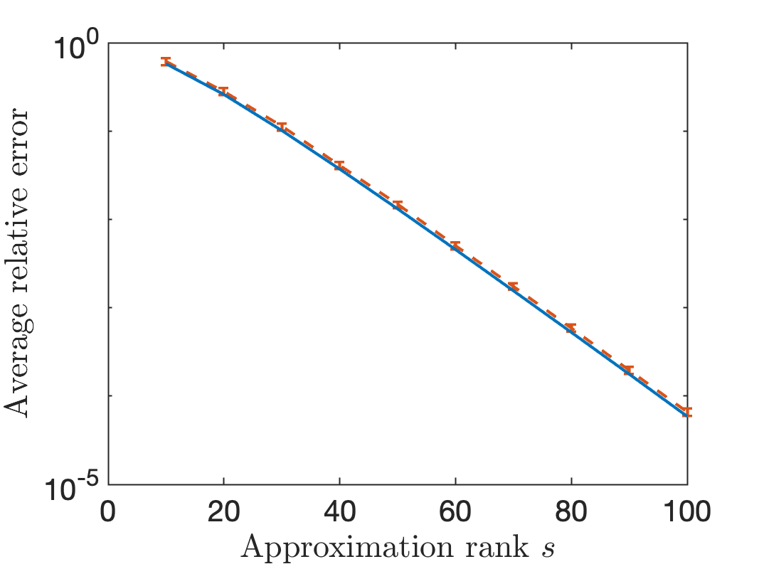
PolyDecay$(p\!=\!2,R\!=\!5)$

NoisyLR$(\xi\!=\!10^{-4},R\!=\!5)$

ExpDecay$(q\!=\!0.05,R\!=\!5)$

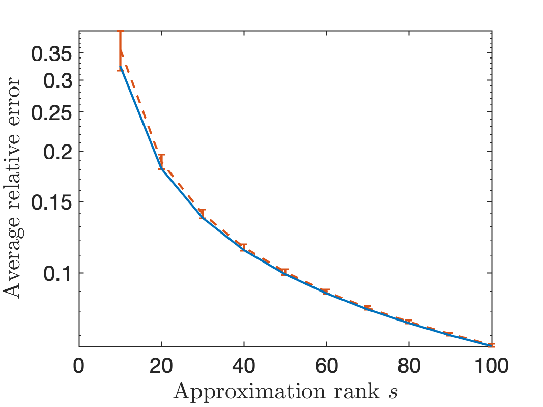
PolyDecay$(p\!=\!1,R\!=\!5)$

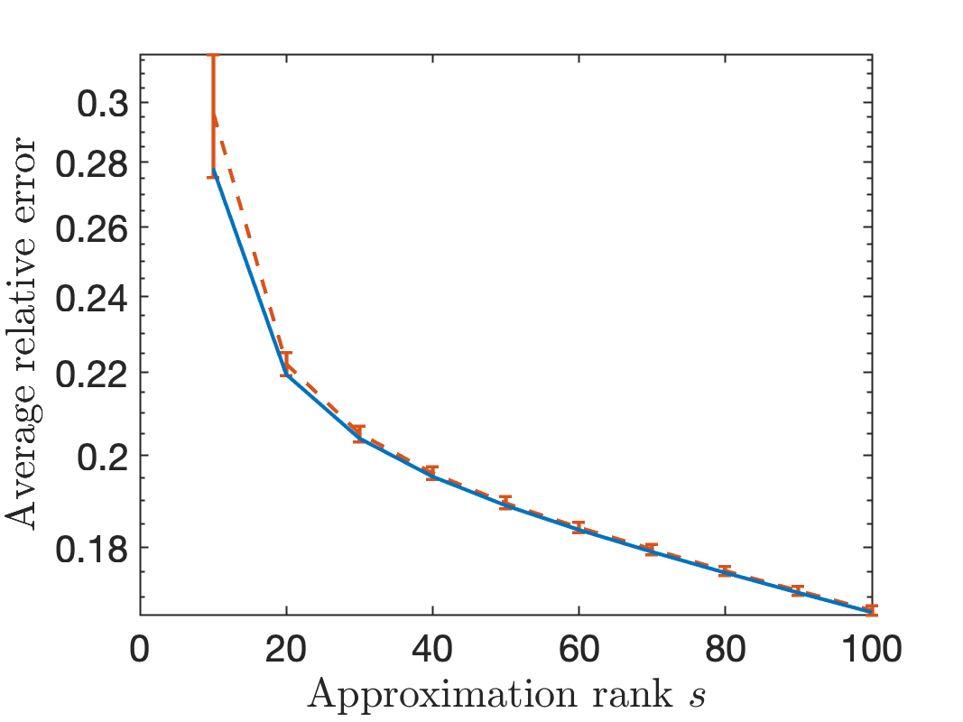
NoisyLR$(\xi\!=\!10^{-2},R\!=\!5)$

Velocity

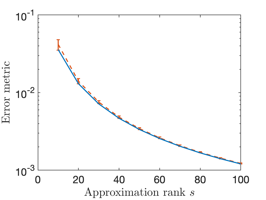
Inverse-Poisson

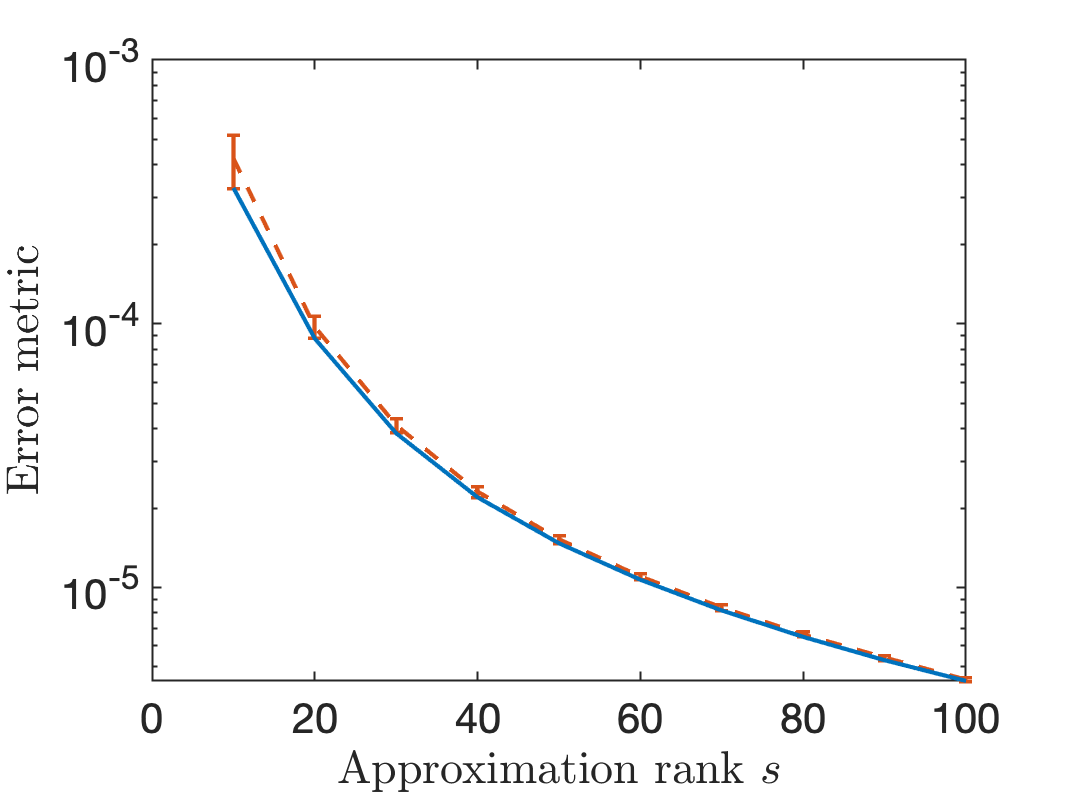
Network

Figure SM1: Leave-one-out error estimator for randomized SVD. Error and error estimate for randomized SVD ($q=0$) approximation. Includes more test matrices than Fig. 3.

ExpDecay$(q\!=\!0.1,R\!=\!5)$

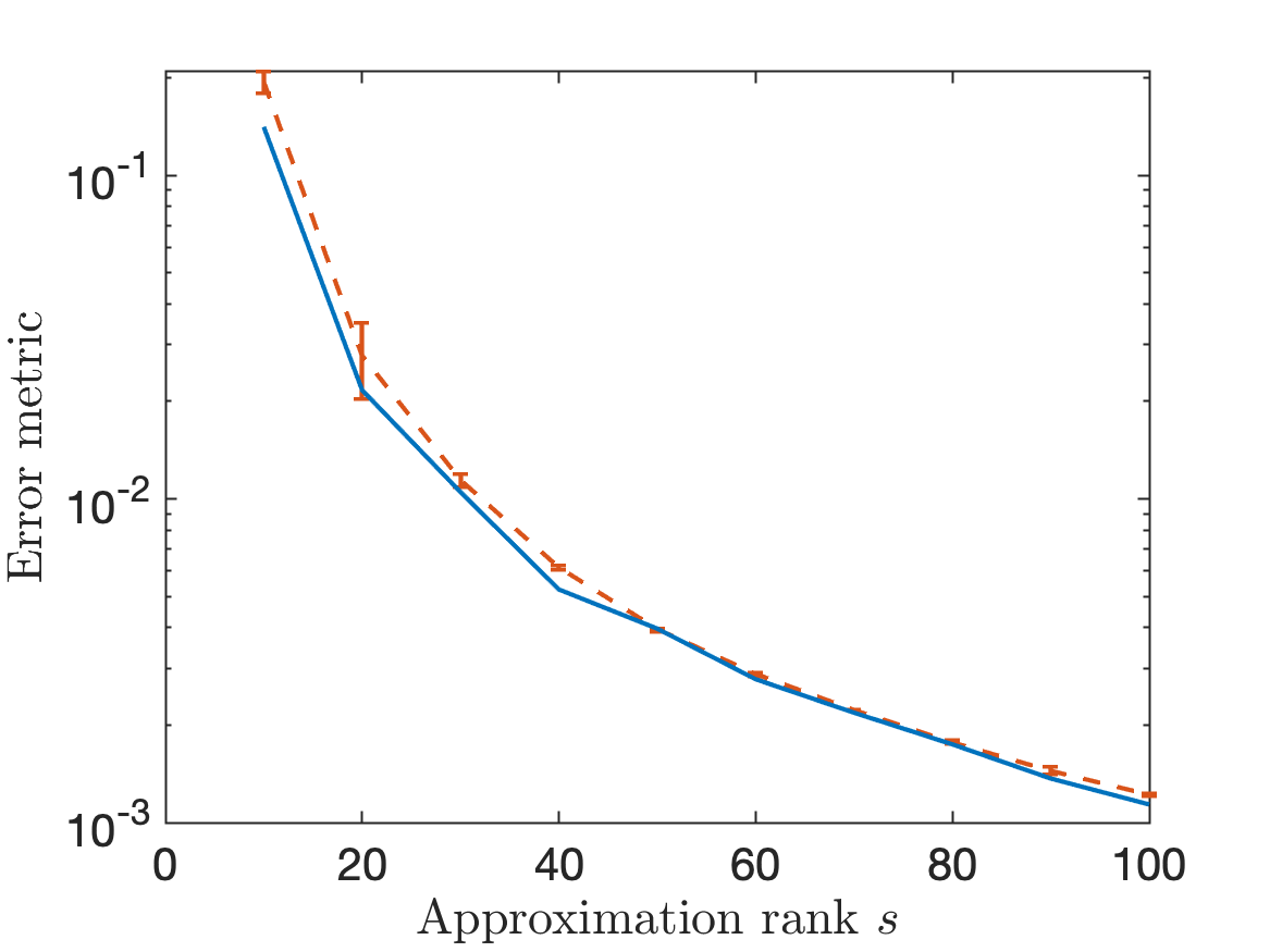
PolyDecay$(p\!=\!2,R\!=\!5)$

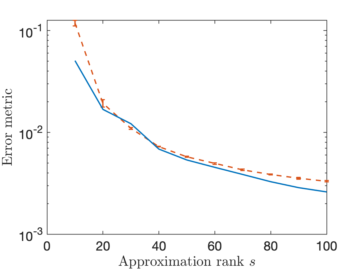
NoisyLR$(\xi\!=\!10^{-4},R\!=\!5)$

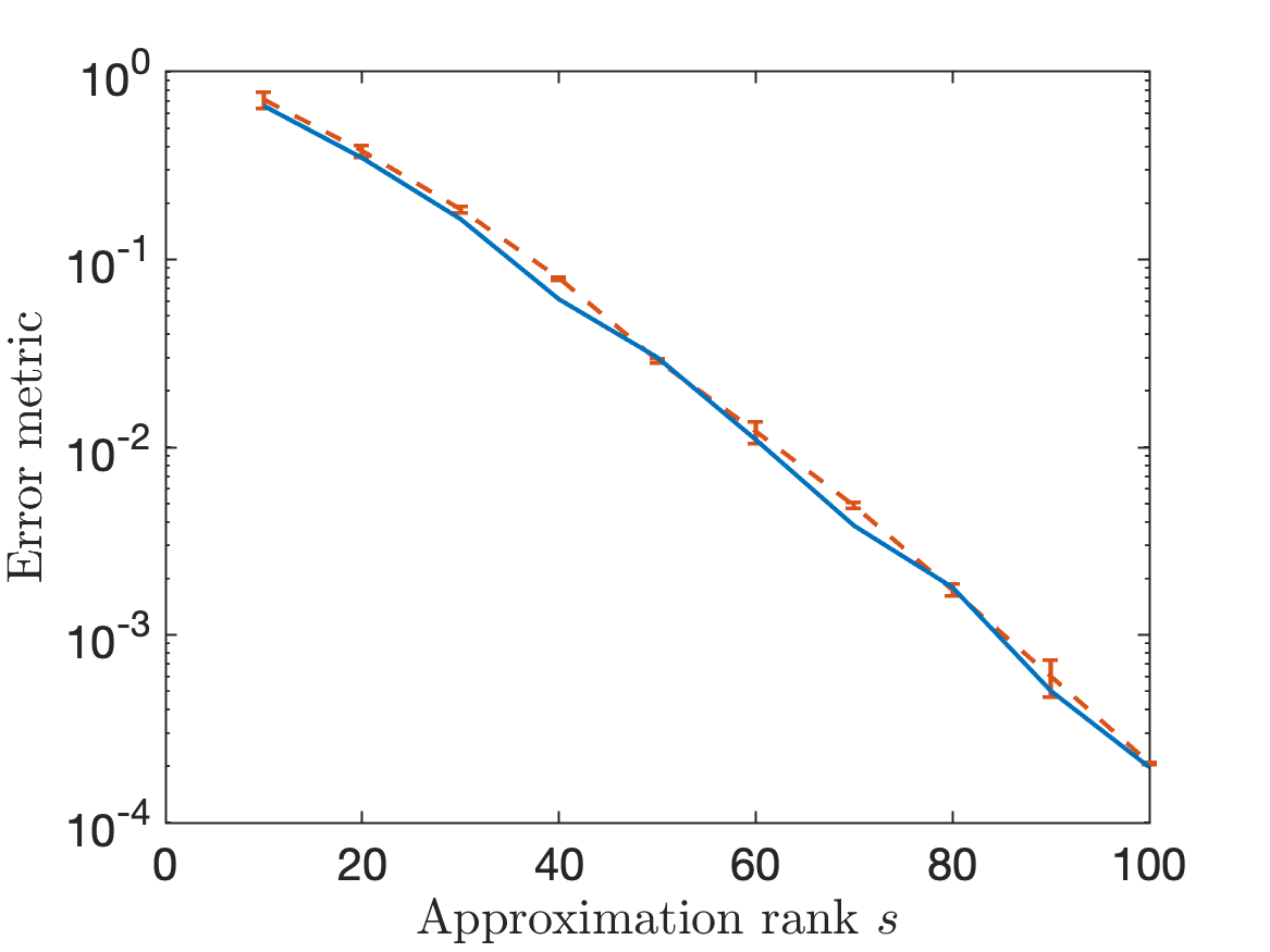
ExpDecay$(q\!=\!0.05,R\!=\!5)$

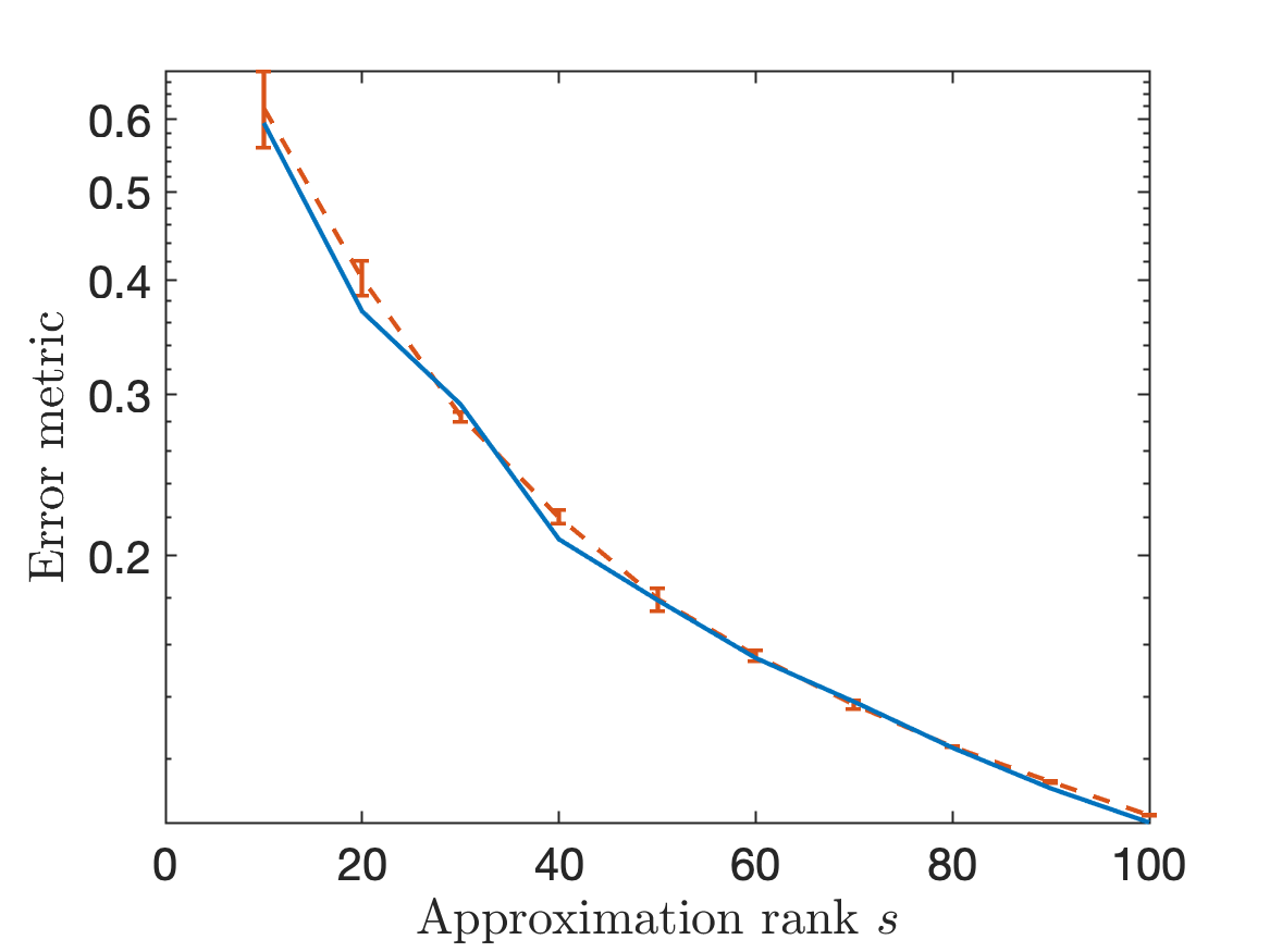
PolyDecay$(p\!=\!1,R\!=\!5)$

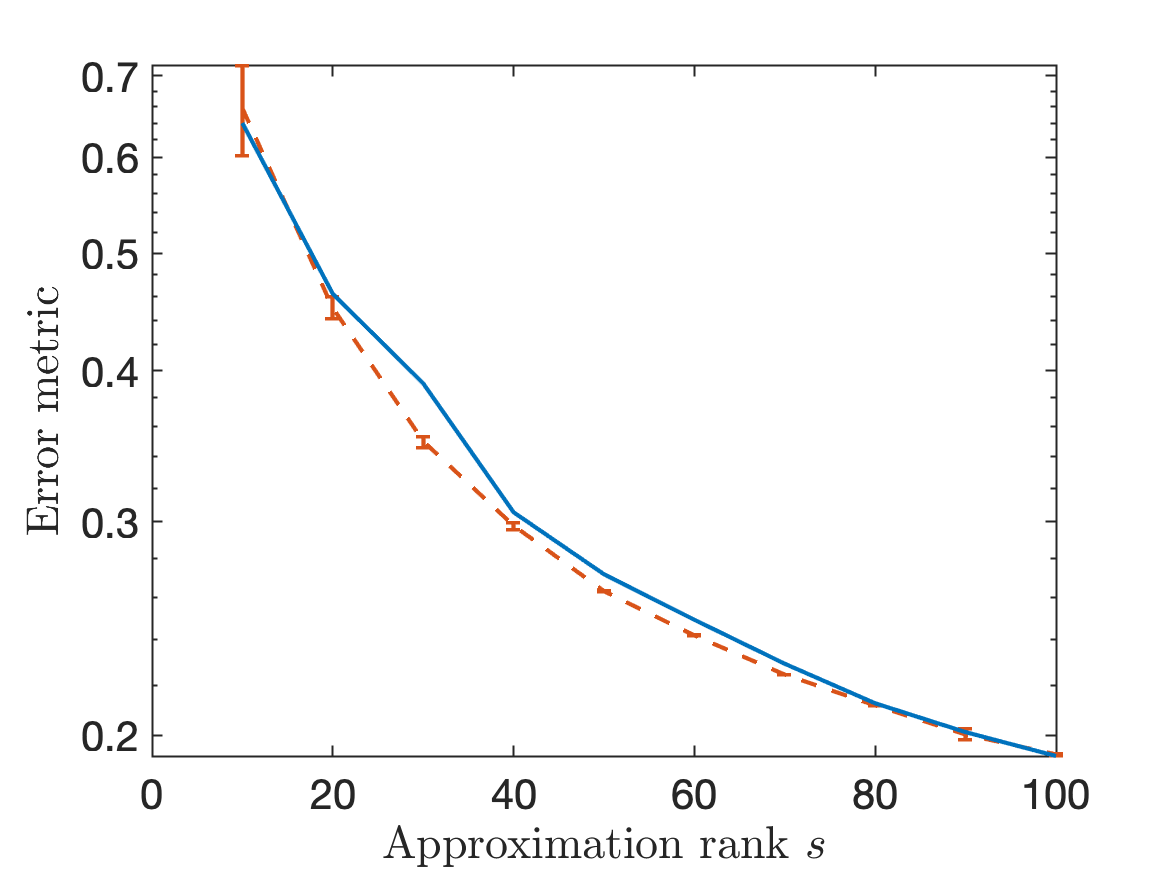
NoisyLR$(\xi\!=\!10^{-2},R\!=\!5)$

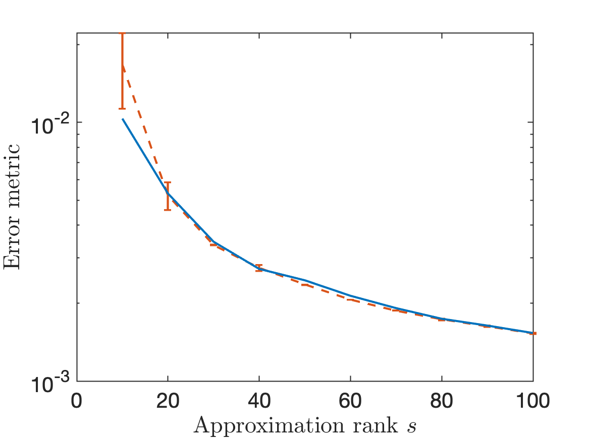
Kernel

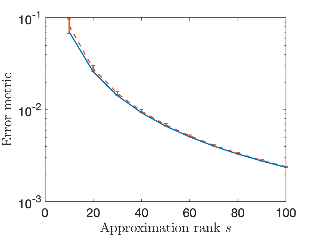
Inverse-Poisson

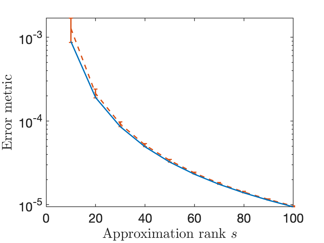
Network

Figure SM2: Leave-one-out error estimator for randomized Nyström. Error and error estimate for randomized Nyström approximation ($q=0$).

ExpDecay$(q\!=\!0.1,R\!=\!5)$

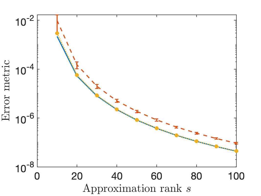
PolyDecay$(p\!=\!2,R\!=\!5)$

NoisyLR$(\xi\!=\!10^{-4},R\!=\!5)$

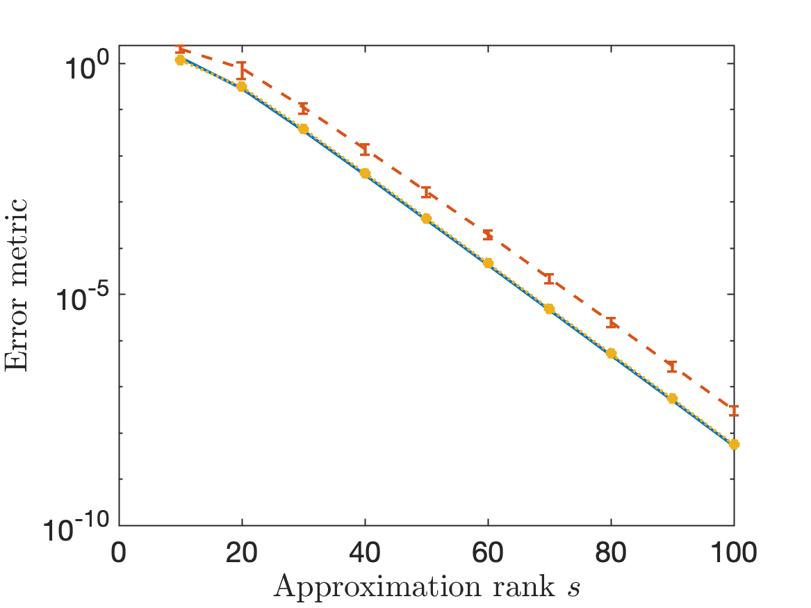
ExpDecay$(q\!=\!0.05,R\!=\!5)$

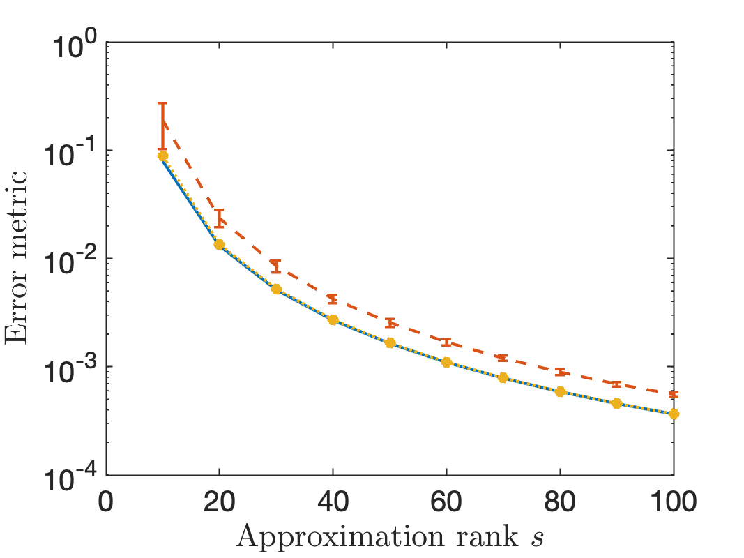
PolyDecay$(p\!=\!1,R\!=\!5)$

NoisyLR$(\xi\!=\!10^{-2},R\!=\!5)$

Velocity

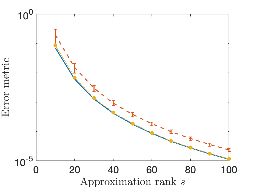
Inverse-Poisson

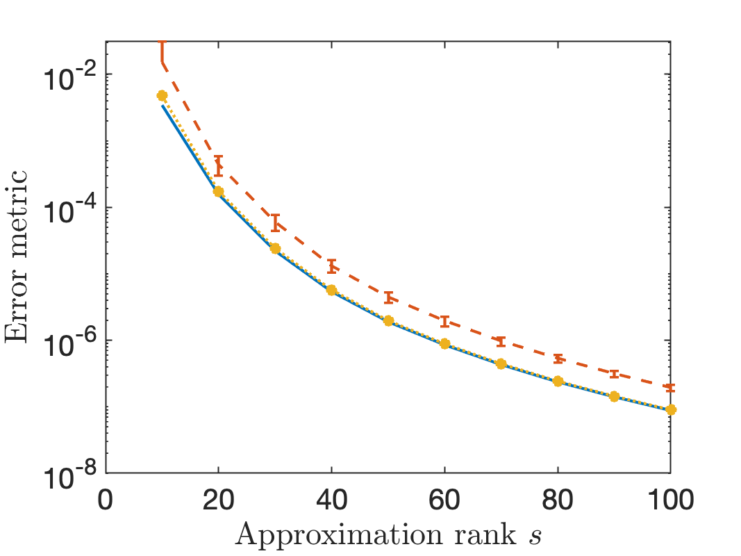
Network

Figure SM3: Matrix jackknife for projectors onto singular subspaces. Error, standard deviation, and jackknife estimate for randomized SVD ($q=0$) approximation $\boldsymbol{X}$ to the projector $\boldsymbol{\Pi}$ onto the span of the five dominant right singular vectors Eq. 19. Includes more test matrices than Fig. 4.

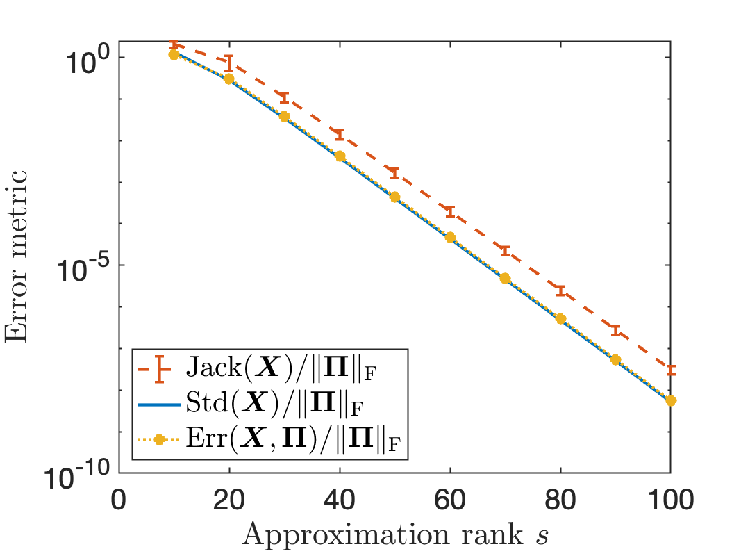
ExpDecay$(q\!=\!0.1,R\!=\!5)$

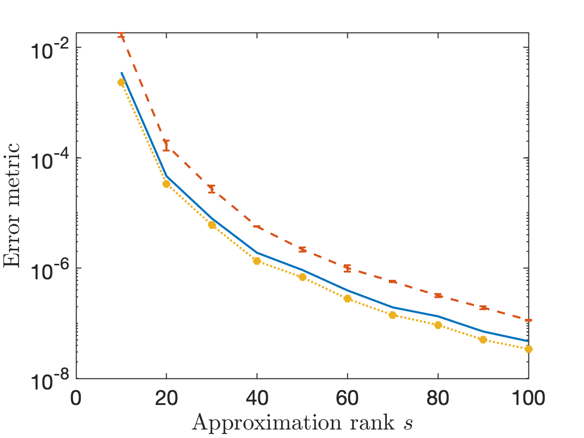
PolyDecay$(p\!=\!2,R\!=\!5)$

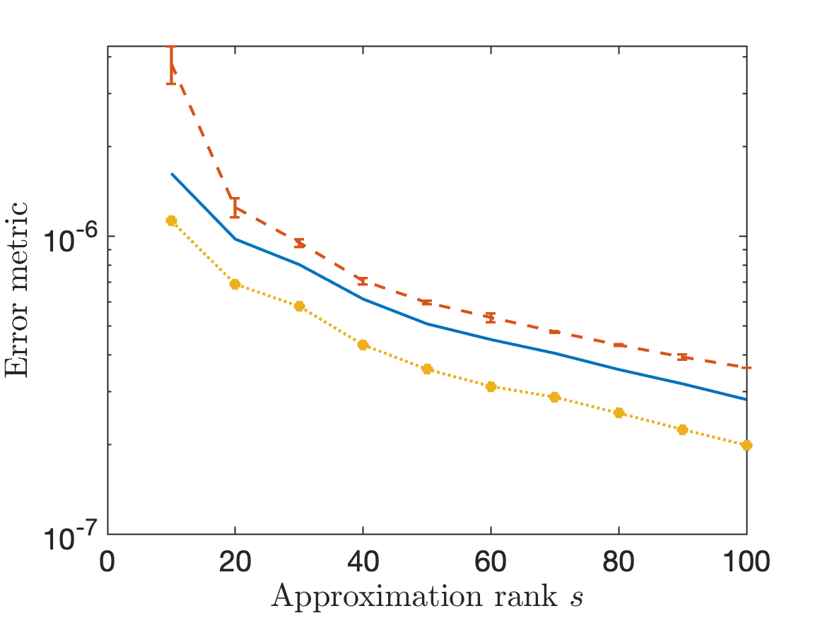
NoisyLR$(\xi\!=\!10^{-4},R\!=\!5)$

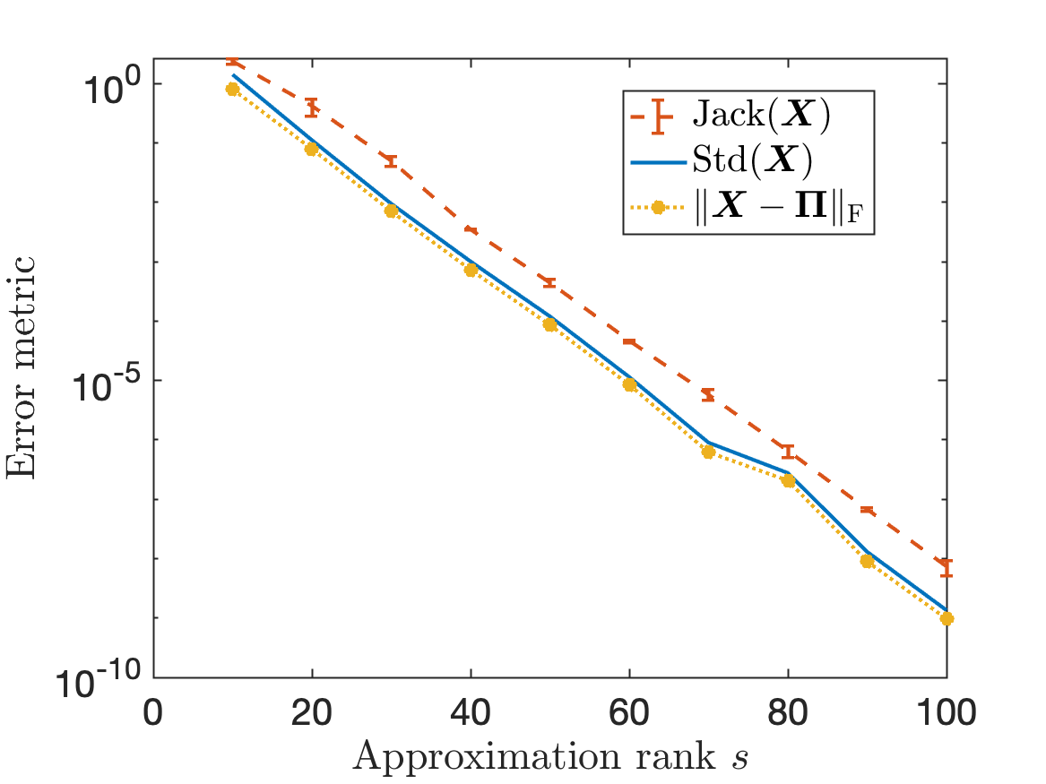
ExpDecay$(q\!=\!0.05,R\!=\!5)$

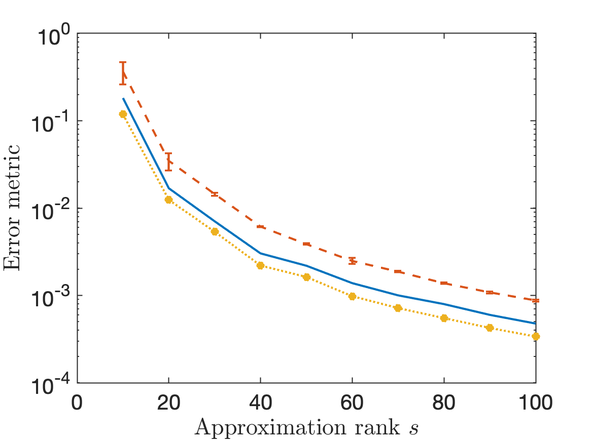
PolyDecay$(p\!=\!1,R\!=\!5)$

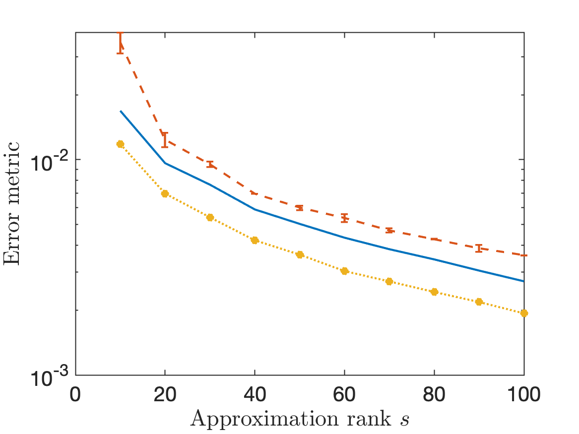
NoisyLR$(\xi\!=\!10^{-2},R\!=\!5)$

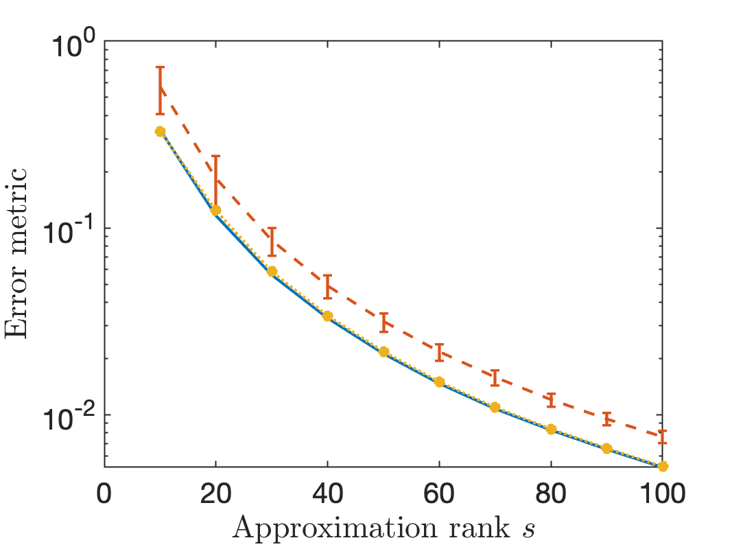
Inverse-Poisson

Network

Figure SM4: Matrix jackknife for spectral projectors. Error, standard deviation, and jackknife estimate for randomized Nyström ($q=0$) approximation $\boldsymbol{X}$ to the projector $\boldsymbol{\Pi}$ onto the span of the five dominant eigenvectors.

Section SM3 MATLAB implementations

In this section, we provide MATLAB R2022b implementations of the leave-one-out error estimate and jackknife variance estimate for the Nyström approximation (Section SM3.1). and randomized SVD (Section SM3.2).

SM3.1 Nyström approximation

LABEL:list:nystrom contains an implementation of Nyström approximation with subspace iteration. This code computes both the leave-one-out error estimate $\widehat{\operatorname{Err}}(\boldsymbol{X},\boldsymbol{A})$ (outputted as err) and the jackknife estimate $\operatorname{Jack}(\boldsymbol{F}(\boldsymbol{X}))$ (outputted as jack) of a transformation $\boldsymbol{F}(\boldsymbol{X})$ of the Nyström approximation. We assume the transformation $\boldsymbol{F}$ takes the form

$$\boldsymbol{F}(\boldsymbol{X}^{(j)})=\boldsymbol{Q}\cdot\mathtt{transform}(\boldsymbol{W}_{j},\boldsymbol{D}_{j})\cdot\boldsymbol{Q}^{*}\quad\text{for every $j=1,\ldots,s$},$$

where $\boldsymbol{Q}$ is a fixed unitary (usually $\boldsymbol{V}$) independent of $j$ and $(\boldsymbol{W}_{j},\boldsymbol{\Lambda}_{j})$ are the eigendecomposition defined in Eq. 22. Natural examples include spectral projectors $\boldsymbol{X}=\boldsymbol{V}\boldsymbol{\Lambda}\boldsymbol{V}^{*}\mapsto\boldsymbol{V}(:,\mathsf{S})\boldsymbol{V}(:,\mathsf{S})^{*}$ for $\mathsf{S}\subseteq\{1,\ldots,s-1\}$ and truncation to rank $r$, $\boldsymbol{X}\mapsto\left\llbracket\boldsymbol{X}\right\rrbracket_{r}$. We solve Eq. 22 using the LAPACK routine dlaed9, called in MATLAB (LABEL:list:update_eig) via a MEX file (LABEL:list:update_eig_mex). An implementation of the Nyström-accelerated spectral clustering procedure with jackknife variance estimation (Algorithm 3) is also provided in LABEL:list:spectral_clustering.

⬇

function [V,Lambda,err,jack] = nystrom(A,s,q,transform)

%% Nystrom approximation

Omega = randn(size(A,1),s);

if q > 0

Omega0 = Omega; Z = A*Omega; Omega = Z;

end

for i = 2:q

Omega = A*Omega;

end

Y = A*Omega;

nu = eps()*norm(Y);

Y = Y + nu*Omega;

[Q,R] = qr(Y,0);

H = Omega’*Y;

C = chol((H+H’)/2);

[U,Sigma,~] = svd(R/C,’econ’);

Lambda = max(Sigma^2 - nu*eye(s), 0);

V = Q*U;

%% Update formula

diagHinv = diag(inv(H))’;

T = ((U’*R/C)/(C’)) .* diagHinv.^(-0.5);

%% Leave-one-out error estimator

if q ~= 0

VO = V’*Omega0;

err = norm(Z-V*(Lambda*VO)+V*(T.*diag(T’*VO)’),’fro’)/sqrt(s);

else

err = norm(((R/C)/(C’)) ./ diagHinv, ’fro’)/sqrt(s);

end

%% Jackknife variance estimate

replicates = zeros(s,s,s);

lambda = diag(Lambda);

for i = 1:s

[Q,D] = update_eig(lambda, T(:,i), -1);

replicates(:,:,i) = transform(Q,D);

end

jack = norm(replicates - mean(replicates, 3), ’fro’);

end

Program 1: nystrom.m: Nyström approximation with leave-one-out error estimator and jackknife variance estimate

⬇

function [Q,D] = update_eig(d,v,c)

%% Negate, sort, and normalize

negative = c < 0;

if negative; d = -d; c = -c; end

[d,p] = sort(d,’ascend’);

v = v(p);

c = c * norm(v)^2;

v = v / norm(v);

%% Compute update

try

[Q,D] = update_eig_mex(d,v,c);

catch ME

if strcmp(ME.identifier, "MATLAB:UndefinedFunction")

error([’Need to build MEX function ’...

’"mex -v update_eig_mex.c -lmwlapack"’])

else

rethrow(ME)

end

end

%% Undo negation and sorting

Q(p,:) = Q;

if negative; D = -D; end

D = diag(D);

end

Program 2: update_eig.m: Solve the updated eigenvalue problem Eq. 22

⬇

// update_eig_mex.c

#include "mex.h"

#include "lapack.h"

void mexFunction(int nlhs, mxArray *plhs[], int nrhs, const mxArray *prhs[])

{

#if MX_HAS_INTERLEAVED_COMPLEX

mxDouble *d, *v, *c, *Q, *l;

#else

double *d, *v, *c, *Q, *l;

#endif

ptrdiff_t n; /* matrix dimensions */

#if MX_HAS_INTERLEAVED_COMPLEX

d = mxGetDoubles(prhs[0]); v = mxGetDoubles(prhs[1]);

c = mxGetDoubles(prhs[2]);

#else

d = mxGetPr(prhs[0]); v = mxGetPr(prhs[1]);

c = mxGetPr(prhs[2]);

#endif

n = mxGetM(prhs[0]);

/* create output matrix C */

plhs[0] = mxCreateDoubleMatrix(n, n, mxREAL);

plhs[1] = mxCreateDoubleMatrix(n, 1, mxREAL);;

#if MX_HAS_INTERLEAVED_COMPLEX

Q = mxGetDoubles(plhs[0]); l = mxGetDoubles(plhs[1]);

#else

Q = mxGetPr(plhs[0]); l = mxGetPr(plhs[1]);

#endif

double *work = malloc(sizeof(double) * n*n);

ptrdiff_t info; ptrdiff_t one = 1;

/* Pass arguments to Fortran by reference */

dlaed9(&n, &one, &n, &n, l, work, &n, c, d, v, Q, &n, &info);

free(work);

}

Program 3: update_eig_mex.c: MEX file to solve the updated eigenvalue problem Eq. 22

⬇

function [clusters, jack, coords] = spectral_clustering(pts,sigma,l,s,q)

%% Set up

K = kernelexp(-pdist2(pts,pts,"euclidean").^2 / (2*sigma^2));

d = sum(K, 2);

A = d.^(-0.5) .* (K .* (d’).^(-0.5));

%% Nystrom approximation

Omega = randn(size(A,1),s);

for i = 1:q

Omega = A*Omega;

end

Y = A*Omega;

nu = eps()*norm(Y);

Y = Y + nu*Omega;

[Q,R] = qr(Y,0);

H = Omega’*Y;

C = chol((H+H’)/2);

[U,Sigma,~] = svd(R/C,’econ’);

lambda = max(diag(Sigma).^2 - nu, 0);

V = Q*U;

%% Spectral clustering

coords = d.^(-0.5).*V(:,1:l);

clusters = kmeans(coords, l);

%% Jackknife variance estiamte

G = V’ * (V ./ d);

diagHinv = diag(inv(H))’;

T = (U’*R/H) .* diagHinv.^(-0.5);

replicates = zeros(s,l,s); avg = zeros(s);

for i = 1:s

Q = update_eig(lambda,T(:,i),-1);

Q = Q(:,1:l);

Q = Q / sqrt(norm(Q’*G*Q,’fro’));

replicates(:,:,i) = Q;

avg = avg + Q*Q’/s;

end

GavgG = G*avg*G;

jack = s * trace(GavgG*avg);

for i = 1:s

Q = replicates(:,:,i);

jack = jack - 2*trace(Q’*GavgG*Q) + norm(Q’*G*Q, ’fro’)^2;

end

jack = sqrt(jack);

end

Program 4: spectral_clustering.m: Spectral clustering with jackknife variance estimation, implementing algorithm Algorithm 3

SM3.2 Randomized SVD

LABEL:list:randsvd contains an implementation of the randomized SVD with subspace iteration. This code computes both the leave-one-out error estimate $\widehat{\operatorname{Err}}(\boldsymbol{X},\boldsymbol{A})$ (outputted as err) and the jackknife estimate $\operatorname{Jack}(\boldsymbol{F}(\boldsymbol{X}))$ (outputted as jack) of a transformation $\boldsymbol{F}(\boldsymbol{X})$ of the randomized SVD approximation. We assume the transformation $\boldsymbol{F}$ takes the form

$$\boldsymbol{F}(\boldsymbol{X}^{(j)})=\boldsymbol{Q}_{1}\cdot\mathtt{transform}(\boldsymbol{U}_{j},\boldsymbol{\Sigma}_{j},\boldsymbol{V}_{j})\cdot\boldsymbol{Q}_{2}^{*}\quad\text{for every $j=1,\ldots,s$},$$

where $\boldsymbol{Q}_{1}$ and $\boldsymbol{Q}_{2}$ are fixed unitaries independent of $j$ and $\boldsymbol{U}_{j},\boldsymbol{\Sigma}_{j},\boldsymbol{V}_{j}$ are defined in Eq. 24. Natural examples include projectors onto left singular subspaces ($\boldsymbol{Q}_{1}=\boldsymbol{Q}_{2}=\boldsymbol{U}$), right singular subspaces ($\boldsymbol{Q}_{1}=\boldsymbol{Q}_{2}=\boldsymbol{V}$), and the truncation of $\boldsymbol{X}$ to rank $r<s$ ($\boldsymbol{Q}_{1}=\boldsymbol{U}$, $\boldsymbol{Q}_{2}=\boldsymbol{V}$). We have not implemented the algorithm of [10] to solve Eq. 24 in $\mathcal{O}(s^{2})$ operations.

⬇

function [U,S,V,err,jack] = randsvd(A,s,q,transform)

%% Randomized SVD

Omega = randn(size(A,2),s);

Z = A*Omega; Y = Z;

for iter = 1:q

Y = A*(A’*Y);

end

[Q,R] = qr(Y,0);

C = Q’*A;

[W,S,V] = svd(C,’econ’);

U = Q * W;

%% Leave-one-out error estimator

T = cnormc(inv(R’));

if q ~= 0

QZ = Q’*Z;

err = norm(Z-Q*QZ+Q*T.*(diag(T’*QZ).’),’fro’)/sqrt(s);

else

err = norm(1./vecnorm(inv(R’)))/sqrt(s);

end

%% Jackknife variance estimate

WT = W’*T;

replicates = zeros(s,s,s);

for i = 1:s

[UU,SS,VV] = svd(S - WT(:,i)*(WT(:,i)’*S));

replicates(:,:,i) = transform(UU,SS,VV);

end

jack = norm(replicates - mean(replicates, 3), ’fro’);

end

Program 5: randsvd.m: Randomized SVD with leave-one-out error estimator and jackknife variance estimate

References

- [1] D. Arthur and S. Vassilvitskii, k-means++: the advantages of careful seeding, in Proceedings of the eighteenth annual ACM-SIAM symposium on Discrete algorithms, SODA ’07, USA, Jan. 2007, Society for Industrial and Applied Mathematics, pp. 1027–1035.
- [2] D. Bu, Y. Zhao, L. Cai, H. Xue, X. Zhu, H. Lu, J. Zhang, S. Sun, L. Ling, N. Zhang, G. Li, and R. Chen, Topological structure analysis of the protein–protein interaction network in budding yeast, Nucleic Acids Research, 31 (2003).
- [3] T. Davis and Y. Hu, The University of Florida sparse matrix collection, ACM Transactions on Mathematical Software (TOMS), 38 (2011), pp. 1–25.
- [4] J. W. Demmel, Applied numerical linear algebra, SIAM, 1997.
- [5] P. Drineas and M. W. Mahoney, RandNLA: Randomized numerical linear algebra, Communications of the ACM, 59 (2016), pp. 80–90.
- [6] B. Efron, The Jackknife, the Bootstrap and Other Resampling Plans, SIAM, 1982.
- [7] B. Efron and C. Stein, The jackknife estimate of variance, The Annals of Statistics, 9 (1981), pp. 586–596.
- [8] E. N. Epperly, J. A. Tropp, and R. J. Webber, XTrace: Making the most of every sample in stochastic trace estimation, Jan. 2023, https://arxiv.org/abs/2301.07825v1.
- [9] A. Gittens and M. Mahoney, Revisiting the Nyström method for improved large-scale machine learning, in Proceedings of the 30th International Conference on Machine Learning, PMLR, 2013, pp. 567–575.
- [10] M. Gu and S. C. Eisenstat, Downdating the Singular Value Decomposition, SIAM Journal on Matrix Analysis and Applications, 16 (1995).
- [11] N. Halko, P.-G. Martinsson, and J. A. Tropp, Finding structure with randomness: Probabilistic algorithms for constructing approximate matrix decompositions, SIAM Review, 53 (2011), pp. 217–288.
- [12] H. Li, G. C. Linderman, A. Szlam, K. P. Stanton, Y. Kluger, and M. Tygert, Algorithm 971: An implementation of a randomized algorithm for principal component analysis, ACM transactions on mathematical software, 43 (2017).
- [13] M. Lopes, N. B. Erichson, and M. Mahoney, Error estimation for sketched SVD via the bootstrap, in Proceedings of the 37th International Conference on Machine Learning, vol. 119 of Proceedings of Machine Learning Research, PMLR, 13–18 Jul 2020, pp. 6382–6392.
- [14] M. E. Lopes, N. B. Erichson, and M. W. Mahoney, Bootstrapping the operator norm in high dimensions: Error estimation for covariance matrices and sketching, Bernoulli, 29 (2023), pp. 428–450.
- [15] M. E. Lopes, S. Wang, and M. W. Mahoney, A bootstrap method for error estimation in randomized matrix multiplication, Journal of Machine Learning Research, (2019), p. 40.
- [16] P.-G. Martinsson and J. A. Tropp, Randomized numerical linear algebra: Foundations and algorithms, Acta Numerica, 29 (2020), pp. 403–572.
- [17] C. Musco and C. Musco, Randomized block Krylov methods for stronger and faster approximate singular value decomposition, in Proceedings of the 28th International Conference on Neural Information Processing Systems - Volume 1, NIPS’15, Cambridge, MA, USA, Dec. 2015, MIT Press, pp. 1396–1404.
- [18] D. Paulin, L. Mackey, and J. A. Tropp, Efron–Stein inequalities for random matrices, Annals of Probability, 44 (2016), pp. 3431–3473.
- [19] S. Puntanen and G. P. H. Styan, Historical introduction: Issai Schur and the early development of the Schur complement, in The Schur Complement and Its Applications, F. Zhang, ed., Numerical Methods and Algorithms, Springer US, 2005, pp. 1–16.
- [20] M. H. Quenouille, Approximate tests of correlation in time-series, Journal of the Royal Statistical Society. Series B (Methodological), 11 (1949), pp. 68–84.
- [21] R. Ramakrishnan, P. O. Dral, M. Rupp, and O. A. von Lilienfeld, Quantum chemistry structures and properties of 134 kilo molecules, Scientific Data, 1 (2014), p. 140022.
- [22] L. Ruddigkeit, R. van Deursen, L. C. Blum, and J.-L. Reymond, Enumeration of 166 billion organic small molecules in the chemical universe database GDB-17, Journal of Chemical Information and Modeling, 52 (2012), pp. 2864–2875.
- [23] Y. Saad, Numerical Methods for Large Eigenvalue Problems, Manchester University Press, 1992.
- [24] J. M. Steele, An Efron-Stein inequality for nonsymmetric statistics, Annals of Statistics, 14 (1986), pp. 753–758.
- [25] R. J. Tibshirani and B. Efron, An introduction to the bootstrap, no. 57 in Monographs on statistics and applied probability, CRC Press, 1 ed., 1993.
- [26] J. A. Tropp and R. J. Webber, Randomized algorithms for low-rank matrix approximation: design, analysis, and applictions, Manuscript in preparation, (2023).
- [27] J. A. Tropp, A. Yurtsever, M. Udell, and V. Cevher, Fixed-rank approximation of a positive-semidefinite matrix from streaming data, in Advances in Neural Information Processing Systems, vol. 30, 2017, pp. 1225–1234.
- [28] J. Tukey, Bias and confidence in not quite large samples, Ann. Math. Statist., 29 (1958), p. 614.
- [29] U. Von Luxburg, A tutorial on spectral clustering, Statistics and computing, 17 (2007), pp. 395–416.
- [30] C. K. I. Williams and M. Seeger, Using the Nyström method to speed up kernel machines, in Proceedings of the 13th International Conference on Neural Information Processing Systems, MIT Press, 2000, pp. 661–667.
- [31] D. P. Woodruff, Sketching as a Tool for Numerical Linear Algebra, Foundations and Trends in Theoretical Computer Science, 10 (2014), pp. 1–157.
- [32] J. Yao, N. B. Erichson, and M. E. Lopes, Error estimation for random Fourier features, Feb. 2023, https://arxiv.org/abs/2302.11174v1. Accepted to AISTATS 2023.