Adaptive Edge Content Delivery Networks for Web-Scale File Systems

Abstract

The InterPlanetary File System (IPFS) is an hypermedia distribution protocol, addressed by content and identities. It aims to make the web faster, safer, and more open. The JavaScript implementation of IPFS runs on the browser, benefiting from the mass adoption potential that it yields. Startrail takes advantage of the IPFS ecosystem and strives to further evolve it, making it more scalable and performant through the implementation of an adaptive network caching mechanism. Our solution aims to add resilience to IPFS and improve its overall scalability, by avoiding overloading the nodes providing highly popular content, particularly during flash-crowd-like conditions where popularity and demand grow suddenly. We add a novel crucial key component to enable an IPFS-based decentralized Content Distribution Network (CDN). Following a peer-to-peer architecture, it runs on a scalable, highly available network of untrusted nodes that distribute immutable and authenticated objects which are cached progressively towards the sources of requests.

I Introduction

In the early days, the Internet was basically a mesh of machines whose main purpose was to share academic and research documents. It was predominantly a peer-to-peer system, computers connected to the network played an equal role, each capable of contributing with as much as they utilised. It was only due to network topology constraints, mainly NATs, that users on the World Wide Web lost the ability to directly dial other peers. Struggling to overcome obstacles in interoperability of protocols, the gap between client and server nodes widen and the pattern remained. In this pattern, computers play either the role of a consumer - “client”- or producer - “server” - serving content to the network.

Serving a big client base requires enormous amounts of server resources. As demand grows, performance deteriorates and the system becomes fragile. Moreover, such an architecture is inherently fragile. Every single source of content at the servers is a potential single point of failure that can result in complete failure and lengthy downtime of the system.

To tackle such flaws, technologies like Content Delivery Networks (CDNs) [cdn-survey] emerged to aggregate and multiplex server resources for many sources of content. This way, a sudden burst of traffic could be more easily handled by sharing the load. Such innovations made the early client-server architecture a little more robust, but at considerable cost regarding infrastructure. Still, despite its inefficiency, the client-server model remains dominant today and runs most of the web.

The InterPlanetary File System (IPFS) [ipfs-filecoin-2020] seeks to revert the historic trend of a client-server only Web. It is a decentralized peer-to-peer content-addressed distributed file system that aims to connect all computers offering the same file system. Due to its decentralized nature, IPFS is intrinsically scalable. As more nodes join the network and content demand increases, so does the resource supply. Such a system is inherently fault tolerant and, leveraging economies-of-scale, actually performs better as its size increases. It uses Merkle DAGs[merkledag][merkledag2], data structures to provide immutable, tamper-proof objects that are content addressed.

However, there are some crucial Content Delivery Network enabling features are lacking in IPFS. In particular, the system lacks the capability of swiftly and organically approximate content from the request path, reducing the latency incurred by future requests. It also does not prepare for the provider of an object to serve a sudden flood of requests, thus rendering content actually inaccessible to some/many.

The goal of this work is, by taking advantage of the ecosystem build by IPFS, to develop an extension to IPFS that implements an adaptive distributed cache that will improve the system’s performance, further evolving it. We aim to:

• reduce the overall latency felt by each peer;

• increase the peers’ throughput retrieving content;

• reduce the system’s overall bandwidth usage;

• improve the overall balance in serving popular content by peers;

• finally, improve nodes’ resilience to flash crowds.

In summary, Startrail serves as a key enabling component for an IPFS-based CDN.

The rest of the document is organized as follows. Section  II describes the proposed solution. We address the architecture of IPFS as a starting point to better understand the integration points of the proposed solution. Next, we further describe Startrail’s architecture, its algorithms and data structures. Section III describes the testbed platform used, all the relevant metrics and obtained results. In Section LABEL:sec:rw, we review previous work and systems in relevant related topics. Some concluding remarks and extension proposals are presented in Section LABEL:sec:conc.

II Architecture

We designed Startrail to be an adaptive network cache, one that continually moves content ever closer to a growing source of requests. The goal is reducing on average the time it takes to access content on the network. It does so without requiring intermediate nodes to previously request such content, thus enabling smaller providers to serve bigger crowds, this way addressing the cost and infrastructure barriers-to-entry of typical CDNs. It also aims to be interoperable, i.e. nodes running Startrail need not depend on other nodes to be effective, enabling nodes to contribute to the network even when adoption is not total.

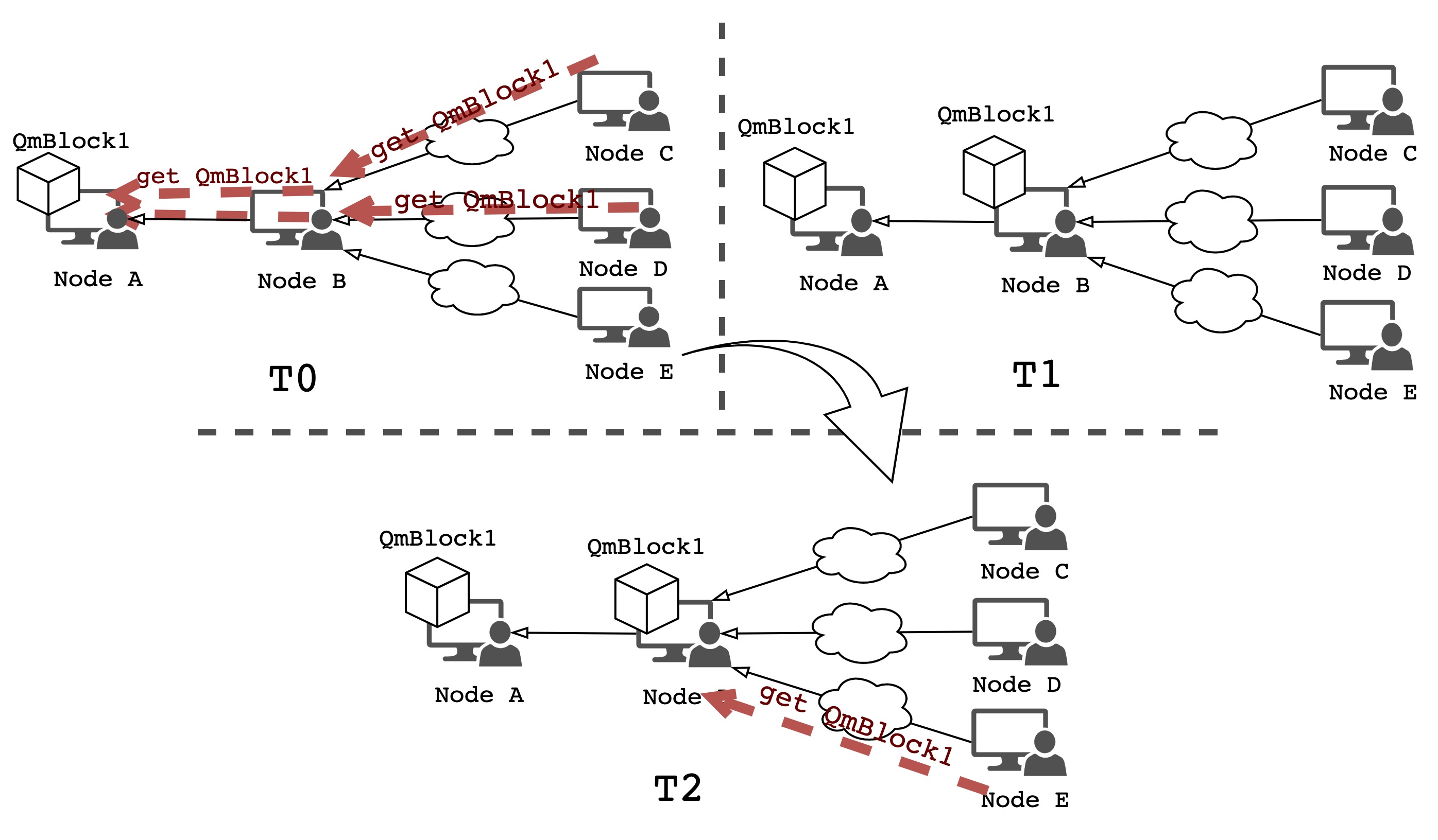
Figure 1: Startrail prototypical example flow

Figure 1 depicts one of simplest scenarios with a small portion of a network where all the nodes are running Startrail: the content, in this case block QmBlock1, is stored on Node A. Nodes C and D request QmBlock1 to the network. While doing so, Node B that is requested by both, detects that the Content Identifier (CID) is popular and flags it, fetching and caching the content itself. Later, when Node E requests the block, the response needs not traverse the whole network, it can be served by Node B.

II-A IPFS Core Architecture

Startrail is built on top of IPFS and integrates with some of its deeper internals and mechanics, thus we address its core. Objects on IPFS consist of Merkle DAGs of content-addressed immutable objects with links, with a construction similar but more general than a Merkle tree [Merkle1988]. Deduplicated, these do not need to be balanced, and non-leaf nodes may contain data. Since they are addressed by content, Merkle DAGs grant tamper proof, which is key to ensure the cached content is genuine. A high-level overview of the architecture of the IPFS core is depicted in Figure 2. We shall delve into each of the illustrated components:

• Core API: the Application Programing Interface (API) exposed by the core, imported by both the Command Line Interface (CLI) and the HTTP API;

• Repo - API responsible for abstracting the datastore or database technology (e.g. Memory, Disk, AWS S3). It aims to enable datastore-agnostic development, allowing datastores to be swapped seamlessly;

• Block: API used to manipulate raw IPFS blocks;

• Files: API used for interacting with the File System. textbfUnixFS is the engine for Unix files layout and chunking mechanisms for network file exchange;

• Bitswap: data trading module for IPFS. It manages requesting and sending blocks to and from other peers in the network. Bitswap has two main jobs: i) to acquire blocks requested by the client from the network; and ii) to send blocks it holds to peers who want them;

• BlockService: content-addressable store for blocks, providing an API for adding, deleting, and retrieving blocks. This service is supported by the Repo and Bitswap APIs.

• libp2p: networking stack and modularized library that grew out of IPFS. It bundles a suite of tools to support the development of large scale peer-to-peer systems. It implements typical P2P mechanisms, e.g. discovery, routing, transport through many specifications, protocols and libraries. One such library is Kad-DHT: the module responsible for implementing the Kademlia DHT [kademlia-02] with the modifications proposed by S/Kademlia [Baumgart2007]. It has tools for peer discovery and content or peer routing.

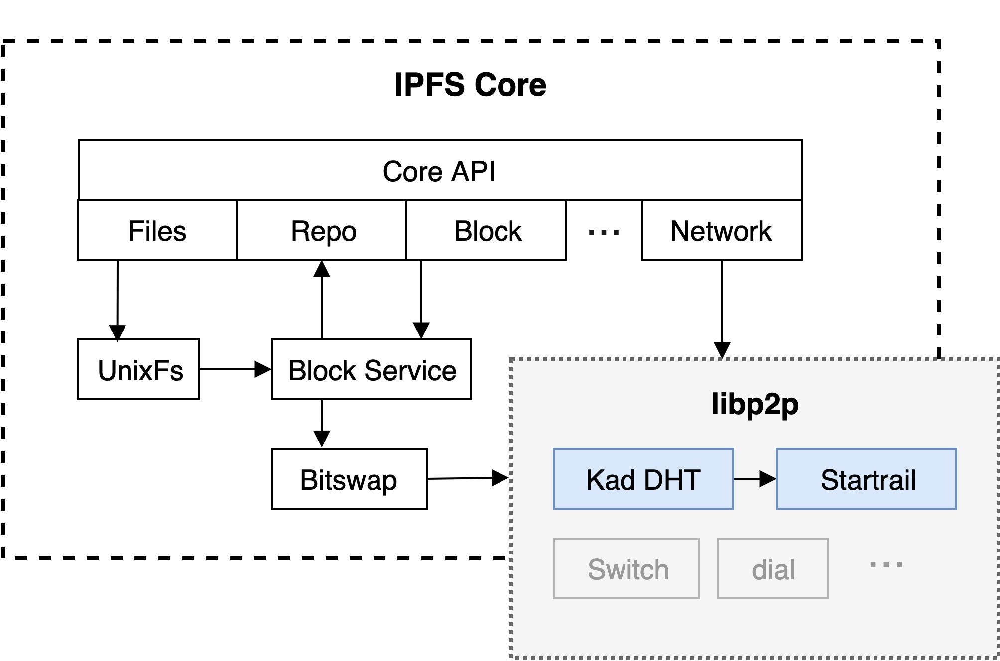
Figure 2: IPFS Core’s Architecture

Data exchanges on IPFS are handled by Bitswap [ipfs-bitswap-2021], a BitTorrent inspired protocol. Peers operate two data-structures:

• want_list: set of blocks a node is looking to acquire;

• have_list: set of blocks a node offers in exchange.

When searching for a block, Bitswap will first search the local BlockService for it. If not found, it will resort to the content routing module, in our case, the Kad-DHT module. This will query the local providers database for the known providers of a certain CID and if not enough are gathered, query the rest from the DHT. Once obtained the set of potential providers, the node will connect to them and pass its want_list containing the target CID (illustrated in Figure 3).

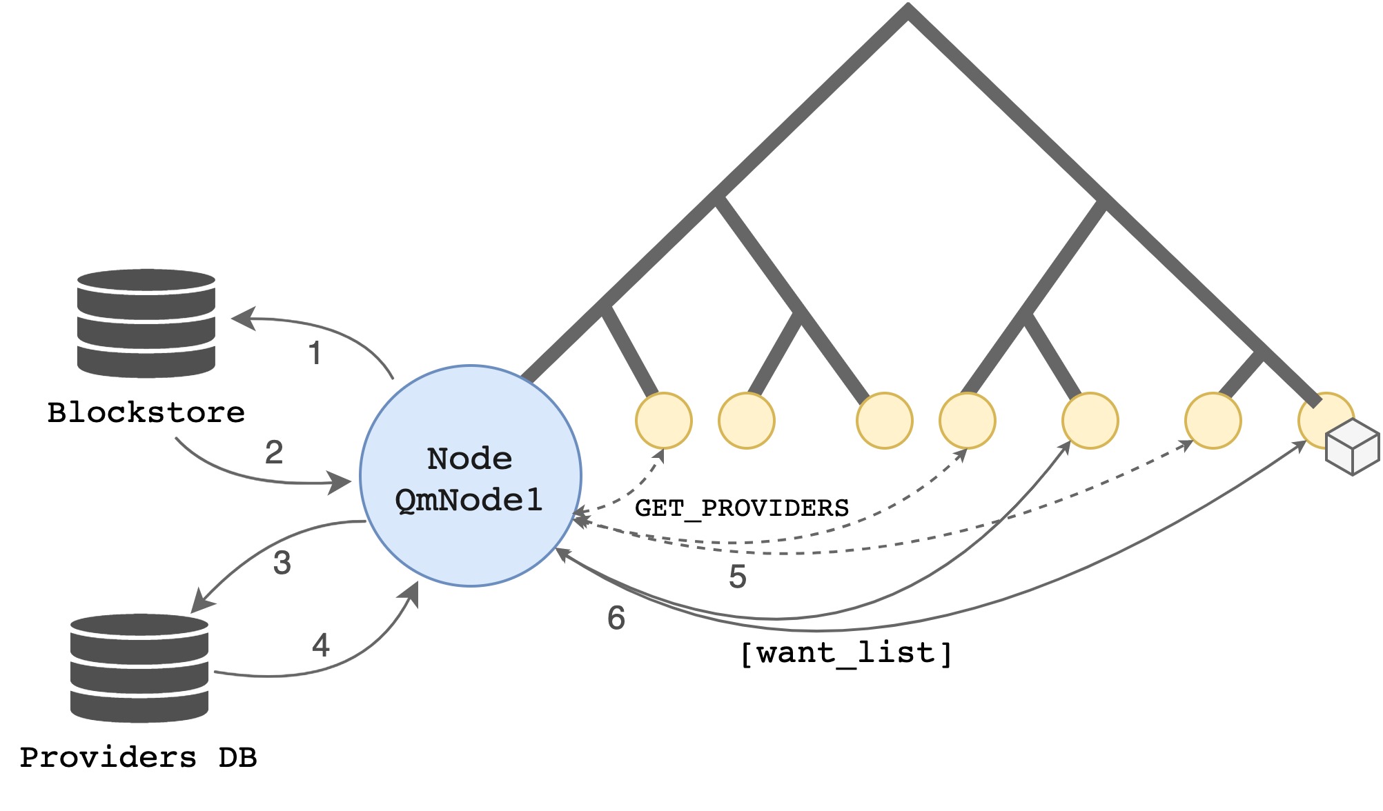
Figure 3: Bitswap-kad-dht interaction when fetching a block from the network

II-B Startrail’s Extension Architecture

We now proceed to describe how and where we integrate the Startrail cache as an IPFS extension to enable CDNs over IPFS. The first step is to identify where to tap into so that new content requests are intercepted. On IPFS, one can do that via two different ways:

• On Kad-DHT, checking for the CID associated to GET_PROVIDER messages;

• On Bitswap, listening for new want_list messages and tracking each of the included CIDs;

Our solution implements the former as it requires addressing just one type of messages.

Startrail’s main activity is to detect trends in object accesses. To do so, it uses two separate components, whose simplified class diagram is depicted in Figure 4:

• Startrail Core: exposing the Startrail API, it is the interface other components will consume to work with StarTrail, It is responsible for integrating with the data trading module (Bitswap), with the BlockService to access data storage, and libp2p for varios network utilities.

• Popularity Manager: component responsible for tracking objects’ popularity. It is totally configurable and it can operate with any specified caching strategy.

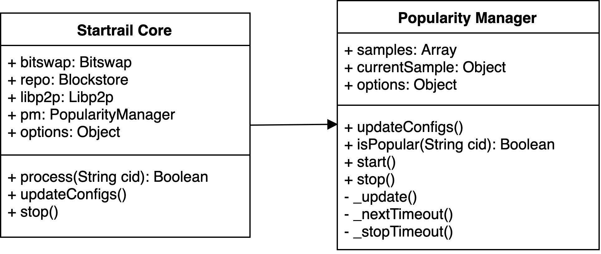
Figure 4: Class diagram of Startrail’s Core and Popularity Manager

The Core includes two main exposed functions: process(cid), responsible for triggering the orchestration and popularity calculation, returning a Boolean for ease of integration with Kad-DHT; updateConfigs(), used for configuration refresh, fetching new configurations from the IPFS Repo and if changes are detected, will update the live ones (useful for hot realoading configurations when testing).

In the Popularity Manager class we find: isPopular(cid), for updating and calculating the popularity for any CID passed as argument; updateConfigs(), serving the same purpose as the above mentioned one; nextTimeout(), managing the sampling timer responsible for scheduling timeouts; update(), runs every time the timeout pops, pushing the current sample to the sampling history and a new one is created.

II-B1 Message processing algorithm

To recognize patterns in object accesses, Startrail examines the CIDs sent on discovery messages. Hence, the process() function is triggered every time the GET_PROVIDER message handler is called. Figure 5 depicts the execution flow starting when a peer requests a block from the network triggering the search for providers on the network. Upon receiving a GET_PROVIDER message, the Kad-DHT handler will execute Startrail’s process hook.

Following the popularity update, either no further action is required, or the block is flagged popular and the peer will attempt to fetch it or retrieve it from the BlockStorage. The block could potentially be found in the storage because, since we are using the IPFS BlockStorage, the block could have been previously fetched by either Startrail or the peer itself. Either way, subsequently to acquiring the block, the peer announces to the network that it is now providing it.

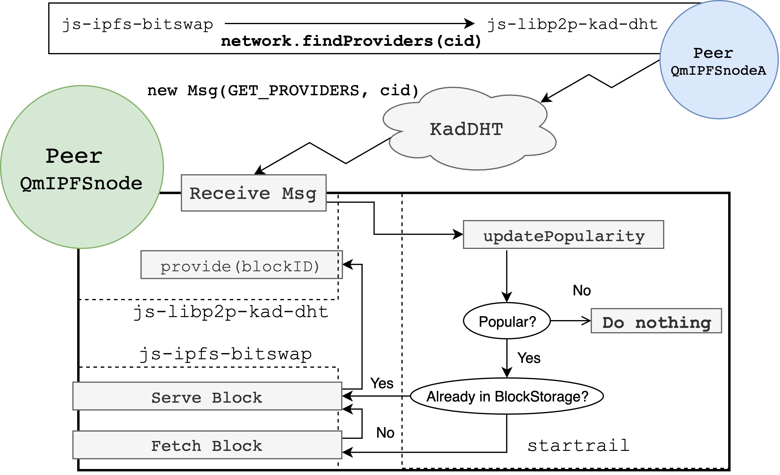
Figure 5: Execution flow inside the Startrail module

II-B2 Popularity Calculation Algorithm

By studying the current and past popularity of a certain CID, we are able to likely forecast content that is going to, at least likely, remain popular in the future. Caching this locally and serving it to other peers has the benefit of making other nodes’ accesses faster. For simplicity, our forecast takes into consideration only a small subset of the node’s past. This subset, or window, can be obtained through various techniques. The one implemented in our solution is a hopping window. Here, sampling windows may overlap. This is desirable in our solution as we want to maintain some notion of continuity and smoothness between samples. Meaning that an object that was popular in the window before, still has high probability to remain popular in the current one, since a portion of the data remains the same. Although parameters are fully configurable, the defaults are 30 seconds for window duration, with hops of 10 seconds.

The Popularity Manager implements the hopping window by dividing it into hop-sized samples. In our case we divide the total 30 second sampling window into three 10 second samples. Every time a new message is processed, the Startrail Core checks the popularity of the referenced object by running the isPopular() function. The function will keep track of objects it has seen in the current 10 second window; incrementing a counter every time the CID processed. Every 10 seconds the current window, or sample expires and is pushed onto a list that holds the previous ones. It is on this latter list of samples (samples in the class diagram Fig. 4) that the popularity calculations are made. An illustration of the interaction between samples and block arrivals is represented on Figure 6.

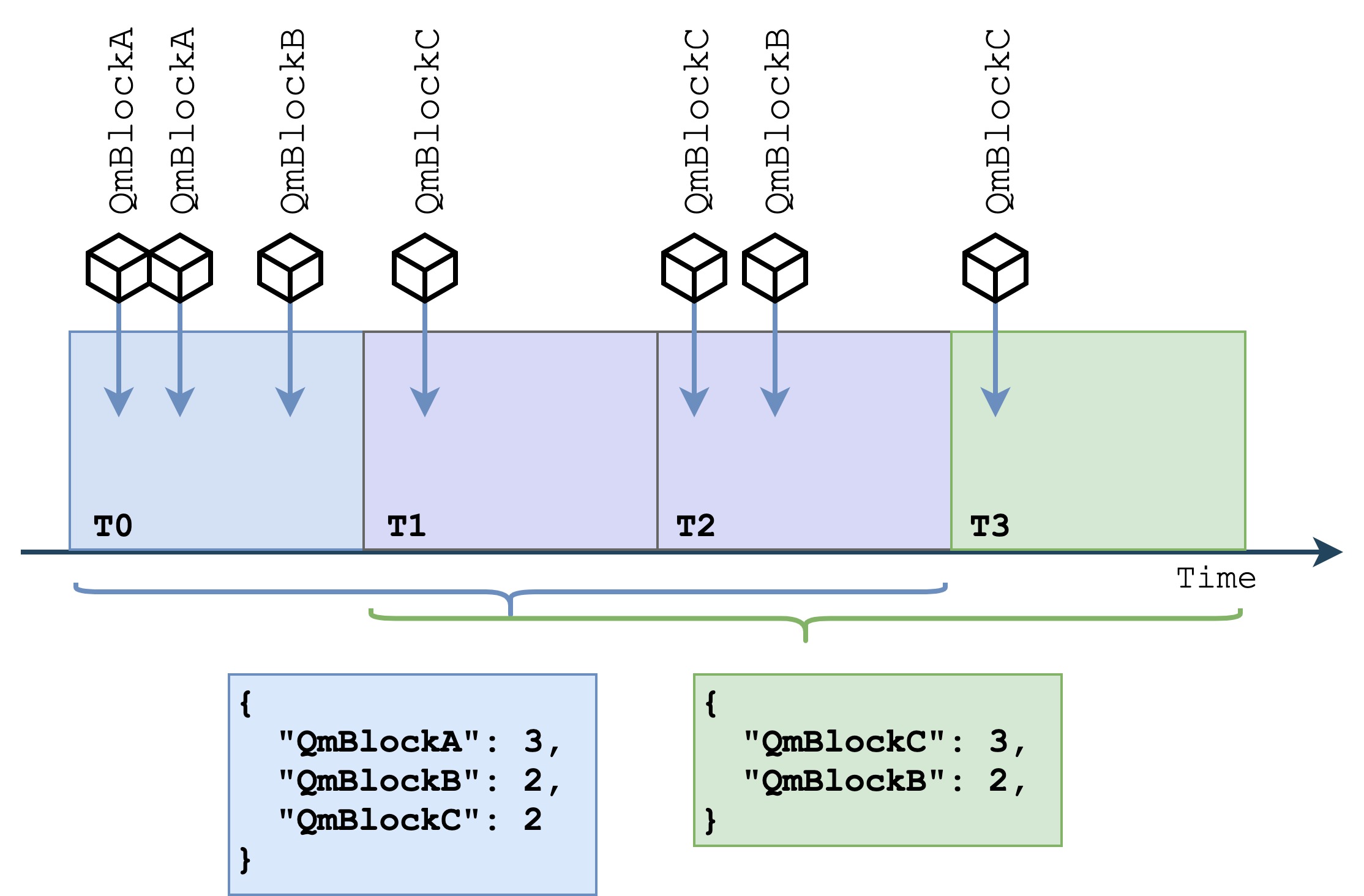
Figure 6: Interaction between new block arrivals and sampling windows

To calculate a block’s popularity the Popularity Manager will first select the three most recent samples after concatenating the current one to this list. Next, it will reduce the array outputting the total amount of times the object was observed. If bigger than a certain configurable threshold the object is considered popular. This heuristic has the benefits of (i) being fairly simple to implement and compute; it also (ii) reacts quickly to changes in content access trends. In out current configuration, it can be considered rather optimistic, since spotting the same object twice will consider it popular.

Our heuristic does not take into account the size of the content being cached. This was a conscious decision, the reasoning for it is that on IPFS most blocks have the maximum default size of 256Kb. Usually only the last one of the sequence that makes up a file is smaller than that. Hence, we disregarded the block size as parameter for caching heuristic.

II-B3 Cache Maintenance

In traditional caching systems [Ali2011], content is always cached by default with the cache replacement algorithm responsible for discarding less relevant documents to create space for new ones. Contrarily, Startrail employs an heuristic to judge which objects should be cached in first place.

We deseign Startrail so that, for the most part, it works by leveraging the internal IPFS mechanics. This ensures the component is lightweight and uses the same procedures as the rest of the system. On Startrail, we allow the node to utilise the full amount of allocated storage by IPFS which defaults to 10 GB. Once it fills up, the IPFS garbage collector (GC) discards unnecessary objects. The IPFS’s GC removes the non-pinned objects. Hence, to prevent popular blocks from being collected when the it executes, we pin the popular objects.

When a block stops being popular it is unpinned, leaving it at the mercy of the GC. When the threshold of 90% of IPFS’ storage is reached blocks are no longer pinned in order to leave room for new blocks.

III Evaluation

III-A The Testbed

There was a considerable amount of effort put into developing a testbed capable of simulating a realistic network. For our specific testbed we were looking for a solution that could fulfill the following requirements:

• enable us to seamlessly adjust and change network conditions, e.g. latency, jitter;

• provide a platform to gather and monitor diverse metrics and logs;

• scale as more computing power is added to the testbed;

• effortlessly enable us to orchestrate and coordinate peers in the networks, i.e execute commands;

• allow for integration with the IPFS codebase. This excluded possible alternatives like PeerSim [Jelasity2009], as this would require porting the whole protocol to the Java API.

III-A1 Testbed Architecture

The complete testbed architecture is depicted on Figure 7. To make the simulations easily reproducible, we leveraged Helm, a tool that helps us release and manage Kubernetes applications. This enabled us to create different node configurations, Charts, and change them for every deployment.

To be able to gather data from different layers of the system during simulations, we resort to the ELK Stack suite of tools. It provides tools for log indexing, searching, transformation, storage and visualisation.

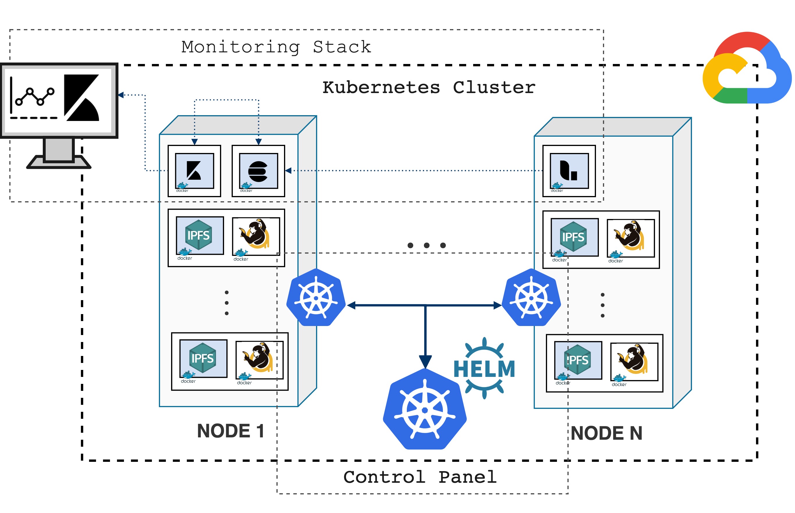
Figure 7: Architecture overview of the testbed network

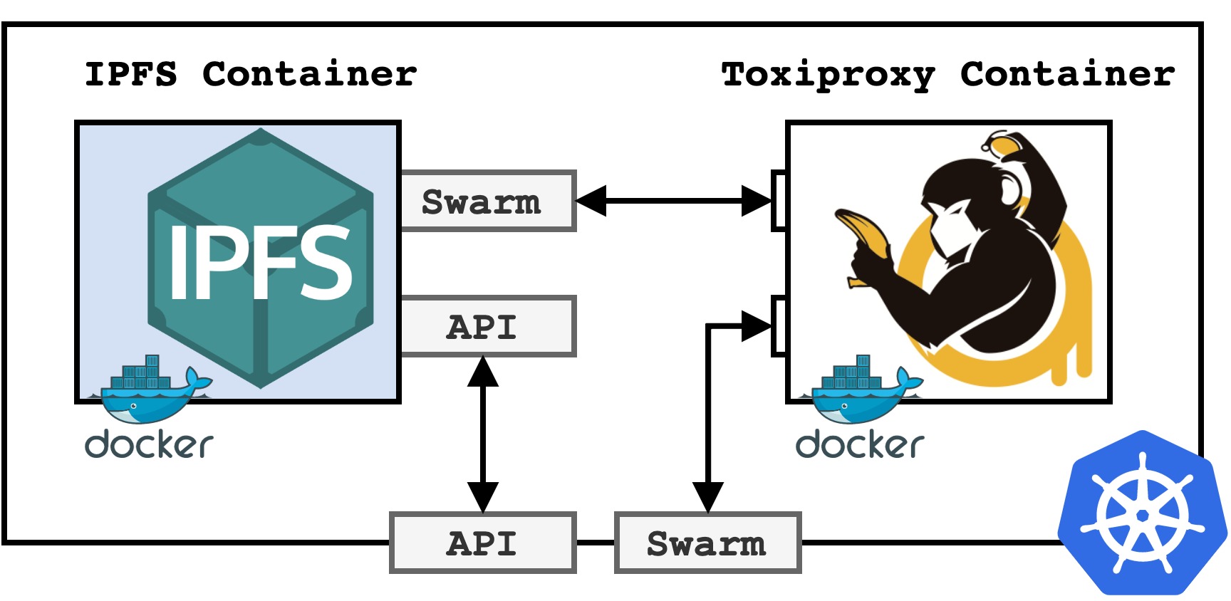
Figure 8: Composition of the Startrail Testbed Kubernetes Pod

To allow for easy addition of computing power into the testbed and management of deployments, we resorted to Kubernetes[kubernetes]. Kubernetes is a tool for deploying and managing containerized applications. It handles the discoverability and liveness of the deployed workloads.

The smallest computing unit on Kubernetes is the Pod. The Pod is a formation of containers, in our case Docker [docker] containers. Our Pod architecture is illustrated in Figure 8. Since Pods allows us to create any arbitrary composition of containers, we took advantage of this and injected, alongside every IPFS node, a Toxiproxy sidecar (a small proxy) from which we channel all IPFS traffic through, coming in and out from the node. This allows us to inject network variability into IPFS connections and simulate diverse network conditions.

III-A2 Deploying a network

We resorted to Unix’s Makefiles to automate the network setup as much as possible, since we were aware that the network would have to be deployed many times. The deployment process, illustrated in Figure 9, is as follows:

• setup Bootstrap nodes: on IPFS, to setup a network we first need to setup the bootstrap peers. These are used by other nodes as a Rendezvous Point to join the network.

• create rest of nodes: additionally, using Helm’s ability to dynamically configure releases, we need to direct these new nodes to the already setup Bootstrap ones.

• deploy Provider nodes: these are nodes preloaded with data. For these, as datasets were sometimes of considerate dimensions, datasets were downloaded onto the Pod from an S3 Bucket before the starting the container.

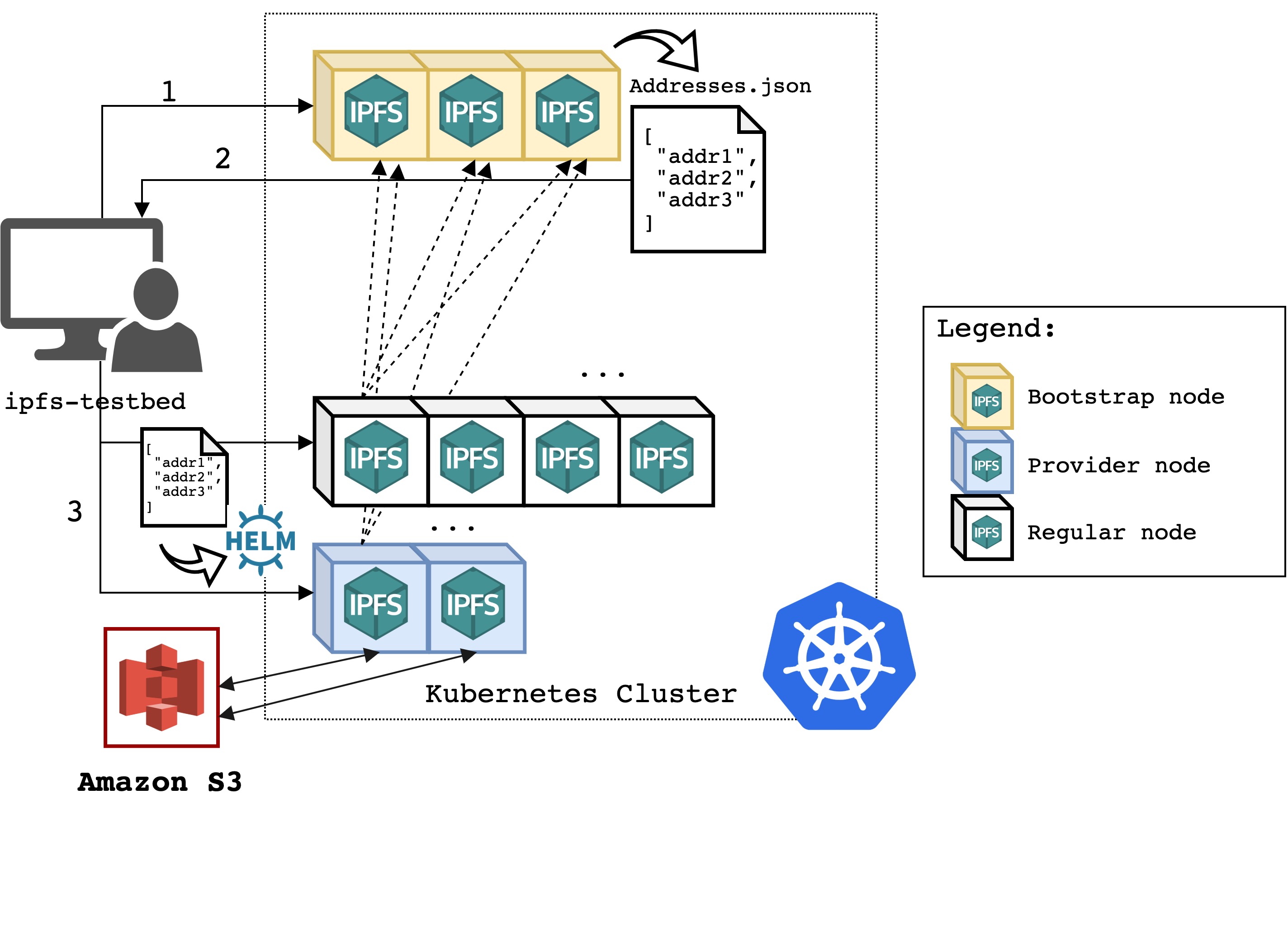
Figure 9: Deployment process of a new network on the Startrail testbed

III-A3 Interacting with the network

To execute our tests, we developed a solution that utilizes the IPFS and Toxiproxy APIs to orchestrate the peers and change the conditions of the network. This interaction can be examined in Figure 10.

With the network in place and a tool with which to execute tests on, it is possible to execute multiple Startrail tests. We executed the tests from our local machine that then would orchestrate commands to each individual peer according to the scripted test file. Using the monitoring platform we then gather live data from the nodes.

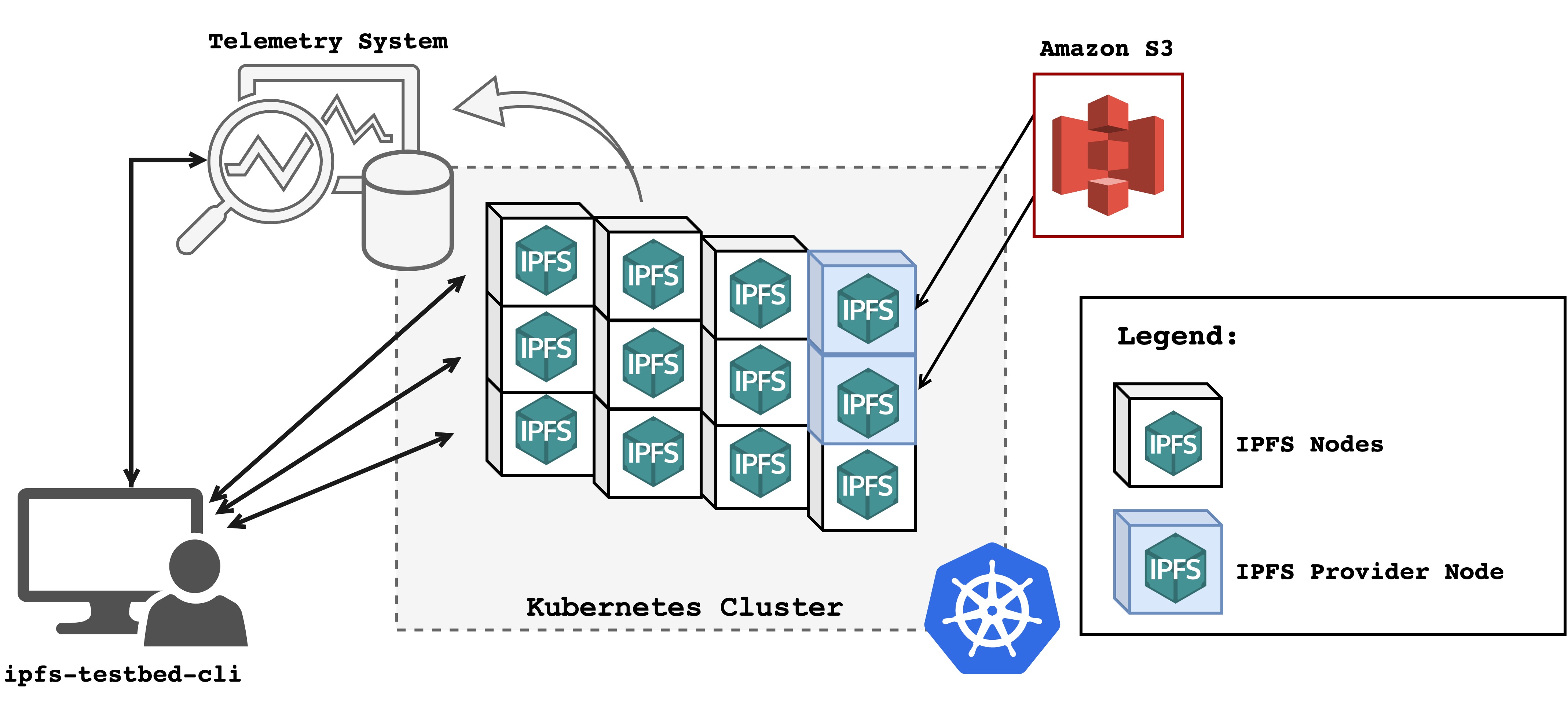
Figure 10: Testbed-cli orchestrating and monitoring Statrail testing cluster

III-B Relevant Metrics

The metrics relevant for Startrail’s performance are:

• request duration: the duration of network request is inherently the most important metric to analyze Startrail’s impact on the system. It can assess if caching mechanism is working and how effective it is. Hence, to measure this we analyze the 95th Percentile request duration.

• memory usage: considering that Startrail Nodes are caching content we want to analyze how much additional data each node has to store.

• network usage: to assess how much each node has to resort to the network in order to fetch content. Hence, we measure the volume of traffic peers send to the network.

For these metrics we calculate the 95th Percentile (95P), that is able to exclude extreme values from the average calculation, the outliers, as do typical cloud provider SLAs.

III-C Testing Setup

The implementation network used to execute the simulations was deployed in the aforementioned Kubernetes cluster running on three n1-standard-4 Virtual Machines on Google Cloud Platform (GCP). These are a general-purpose type of machine with 4 vCPUs, 15 GB of memory and 128 GB of storage, representative of many laptop, desktop, and smaller server machines powering IPFS. With this setup, we were able to simulate a network of 100 peers, of them 5 are bootstrap nodes, and 2 are providers preloaded with data.

To simulate different content access patterns we ran the following request management policies (implemented as functions in the test code) which pick a block from a dataset of thousands and order the peer to fetch it:

• Random Access (RA): the random access policy picks each block with equal probability. This pattern can serve as control;

• Pareto Random (PR): with the Pareto Distribution [Rosen1980] serving as an adequate approximation for Internet objects popularity[pareto], this policy approximates our desired distribution with an alpha equal to 0.3, meaning that 20% of the blocks generate 80% of the overall network traffic;

• File Random (FR): here we divided the total list of blocks into smaller lists, each amounting to 3Mb in block data. Selecting one of these lists means that the peer fetches all the nodes in the list, thus simulating complete file access. We also use a Pareto distribution here.

Table I summarizes all the test scenarios simulated. Each one had an induced latency of 100 ms, ran for 10 minutes and each node requested a new block every 30 seconds.

Test Name	Startrail	Access Type	Window Size	Threshold
RA w/o Startrail	False	RA	N.A.	N.A.
RA w/ Startrail	True	RA	3*10sec	2
PR w/o Startrail	False	PR	N.A.	N.A.
PR w/ Startrail	True	PR	3*10sec	2
FR w/o Startrail	False	FR	N.A.	N.A.
FR w/ Startrail	True	FR	3*10sec	2

TABLE I: Different testing condition for running network tests

The parameter columns are:

• Startrail: defines if Startrail was running on all the nodes in the network;

• Access Type: indicates which of the previously mentioned access patterns we are simulating;

• Latency: the amount of latency introduced by Toxiproxy;

• Req. Freq.: specifies at which frequency the requests for blocks - or array of blocks, in the case of File Random - are made by the individual nodes;

• Duration: indicates for how long we run the simulation;

• Window and Threshold: specify the used Startrail configuration, if applicable. Window being the amount of samples and the duration of each, in seconds; and the Threshold of accesses to trigger caching in Startrail.

III-D Tests Results

III-D1 Latency Analysis

The chart on Figure 11 depicts the calculated 95P Request duration for each simulation. The simulation of the random access running on a regular IPFS nodes’ network, on the far left, yielded a P95 latency of 60 seconds. The same simulation running on the Startrail network only took 40 seconds. This is a considerable reduction of one third. Similar gains in speed can be observed for the tests with Pareto distribution access pattern.

At first glance, one would think that this would be the policy where the impact of Startrail would be the most evident, because the blocks would reach the cache threshold easier, In this case, however, since the same blocks are being requested more often, different peers on the network also serve the content because they previously downloaded it. Hence, the difference remains the same. For the file access type the proportion of gains remains similar, with the overall latency going up since now we are requesting a lot more of different blocks.

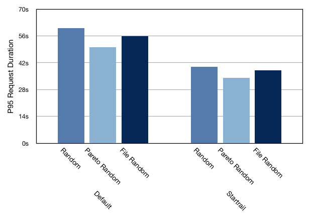
Figure 11: 95th percentile of request duration for the different testing scenarios

III-D2 Memory Consumption Analysis

The chart on Figure 12 compares the memory cost of running the simulations on a network with and without Startrail. Its analysis reveals that running the simulations without Startrail costs generally the same, with only slight variations proportional to the amount of different blocks requested. For the simulations run on the Startrail network we observe a consistent increase in memory utilization. This is expected since nodes are now storing more content, the cached blocks.

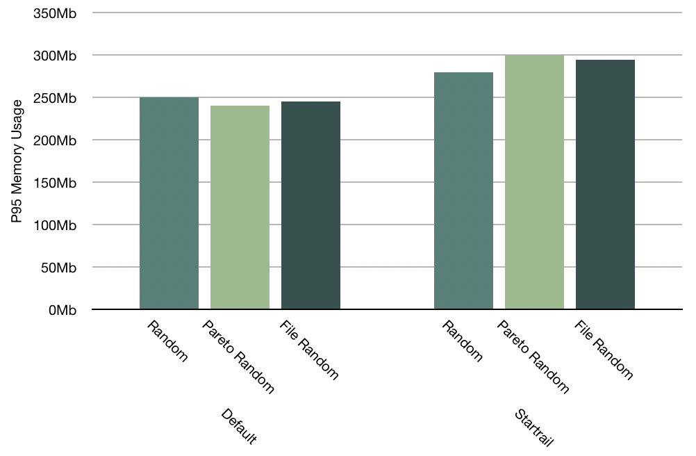
Figure 12: 95th Percentile of memory usage on the different testing scenarios

For the Pareto access pattern we notice an increase in memory consumption relative to the all random ones. This is not completely intuitive, as the smaller diversity of blocks requested could mean less content being cached. However, we find that in this simulation a smaller subset of the dataset is now being constantly requested, meaning that, although smaller, it reaches the cache threshold with a very high probability and is therefore all stored. Additionally, because it doesn’t grow significantly and past the IPFS default 10 GB of storage, the GC is never triggered and thus the cached blocks are kept for the whole duration of the test. This does not happen with the random access pattern because, since it follows a uniform distribution, requests for the same block can be scattered over time and thus some never reach the threshold.

III-D3 Network Consumption Analysis

The chart on Figure 13 illustrates the network impact of running simulations with and without Startrail. Comparison of the obtained results reveals that the savings in network traffic (MBs) are proportional to the speed ups in request latency. This happens because requests are being served closer to their source by caching nodes and thus fewer messages have to transit over the network.

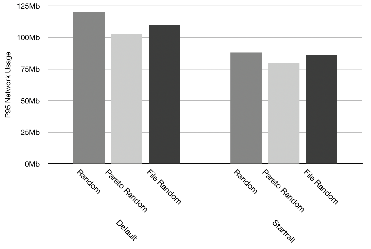
Figure 13: 95th Percentile of network usage on the different testing scenarios

III-D4 Variable Startrail adoption

Additionally, we also analyzed the impact of the percentage of Startrail-enabled nodes in the network. This allows us to assess the interoperability of Startrail with the base IPFS and to confirm their compatibility, which is key for incremental deployment and adoption. Furtermore, it also allows us to determine whether the benefits of Startrail are significant, even if only a smaller percentage of nodes are contributing to caching and if, on the other hand, there is an optimal percentage of Startrail participation in IPFS that would yield the best performance.

In order to evaluate which of the above mentioned propositions were true we ran aditional simulations. The conditions of these were similar to the ones presented earlier: in each test the latency induced was 100, the tests ran for 10 minutes and each node requested a new block every 30 seconds. The distinction between the ones described before and these is that in the latter we alternated the percentage of nodes running Startrail that were deployed on the network. The percentages were: 0%, 30%, 50%, 80% and finally 100% Startrail nodes.

The results obtained from running the simulations were compiled into the chart in Figure LABEL:fig:startrailTestPercentage. The samples start on the far left with higher values of request latency for no Startrail participation on the network, and decrease nearly linearly as the percentage of Startrail nodes increases. Therefore, it appears that the impact of Startrail nodes’ percentage on the network performance can be approximated through the linear regression drawn on the dotted line in the graph. This supports our initial proposition that th performance would improve as the percentage of Startrail nodes increases.

Nevertheless there is a slightly higher slope in the 30% to 50% range. That however does not allow any conclusions of an optimal point to be taken (possibly due to some experimental noise or from the coarse-grained range of the parameter used in the testing but that still highlights the relevant trend).