Quasi Normal Modes of Ayon-Beato Garcia Regular Black Holes For Scalar Field

Abstract

In this paper, we compute quasi-normal modes of ABG black holes (which has a non-linear electrodynamical source) using the WKB methods and AIM. A comparison between the spectrum of QNMs calculated by both methods is made. We analyse how the spectrum of QNMs depends on the black hole parameters, multipole number and overtone number and establish that the ABG black hole is stable against the scalar field.

1 Introduction

Black Holes(BH) are the most radical prediction of Einstein’s General relativity. The study of BH had started in the early 20th century. BH is a very simple object when it’s kept in isolation, and these isolated BHs are characterized by only a few parameters such as their mass, charge and angular momentum. However, a BH cannot be isolated because it interacts with the surrounding astrophysical objects such as accretion disk, stars, planets etc or fields such as scalar field, electromagnetic field, Weyl field. Thus a BH is always in the perturbed state. The perturbed BH responds to perturbations by emitting gravitational waves. The dynamical evolution of these gravitational waves can be conditionally divided into three-stage. Among three divisions of the dynamical evolution of gravitational waves, the damping oscillations of black holes have great interest, known as Quasi- Normal Modes(QNMs) of Black Hole. These QNMs are the dependent of the parameters of BH like mass, charge and angular momentum, of the types of the perturbation like a scalar, electromagnetic etc which are the cause of the excitation of BH. The frequencies of these QNMs are complex, where the real part gives the frequency of the perturbation and the imaginary part gives its damping rate. Since these QNMs depend on the BH parameters, it provides us with lots of information about BH. QNMs are extensively used in conjecture Ads/CFT correspondence Maldacena1999 . The return to thermal equilibrium of the perturbed state in CFT is related to the imaginary part of the QNMs PhysRevD.62.024027 . QNMs are also used to interpret loop quantum gravity BEKENSTEIN19957 ; PhysRevLett.81.4293 ; PhysRevLett.90.081301 and to test different alternative gravity theories.

Regge and Wheeler Regge:1957td were the first persons who discovered that the whole study of perturbation theory of BH could be reduced to a Schrödinger-like equation and their work was extended by Zerilli PhysRevD.2.2141 ; PhysRevLett.24.737 . In 1970, Vishveshwara PhysRevD.1.2870 studied the stability of Schwarzschild metric and showed QNMs behaviour of BH by scattering of gravitational waves Vishveshwara:1970zz . Chandrasekhar and Detweiler proved that the Regge-Wheeler and Zerilli potential are isospectral and also calculated QNMs for Schwarzschild BH, using shooting method Chandrasekhar:1975zza . Hans-Joachim Blome and Bahram Mashhoon BLOME1984231 analytically calculated QNMs of Schwarzschild BH states of the inverted effective potential of BH, an approximation of Eckart potential. In the same year, Ferrari and Mashhoon PhysRevD.30.295 used the same technique to compute QNMs but this time they used Pöshi-Teller potential to approximate inverted BH effective potential. Leaver published series of paper doi:10.1063/1.527130 ; PhysRevD.34.384 ; Leaver:1985ax to calculate QNMs numerically using Continuous Fraction Method (CFM) . Later on some new methods like Horowitz Hubeny method (HH) Horowitz-Hubeny:2000 , asymptotic iteration method (AIM) Cho_2010 were proposed to calculate QNMs numerically. Some review papers Nollert:1999ji ; Kokkotas1999 ; Berti_2009 ; Konoplya:2011qq give a brief description of QNMs and it’s applications. The modified classical general relativity or quantum gravity may give rise to a class of BH with no pathological singular behaviour. These singular BHs are called regular BH Bardeen ; Mars_1996 ; Barrab ; Borde ; AyonBeato:1998ub ; Ayon-Beato1999 ; Ayon-Beato:2000mjt ; PhysRevLett.96.031103 . These regular BHs can be constructed by coupling gravity to matter having non-linear electrodynamic behaviour. Flachi and Lemos PhysRevD.87.024034 , Toshmatove et al. PhysRevD.91.083008 ; Toshmatov:2018ell , Wu refId0 and several other authors like Li:2016oif ; Lopez:2018aec ; Panotopoulos:2019qjk ; PhysRevD.103.124050 found QNMs of regular BHs. Hendi et al. PhysRevD.103.064016 studied the thermodynamic properties of the regular rotating BH using QNMs. Cai and Miac Cai:2020kue studied the regular BH in scalar-tensor-vector gravity. Bronnikov et al. Bronnikov:2012ch showed that the regular BHs and wormholes are unstable against the phantom scalar field except for one special class of black universe. Churilova and Stuchlik Churilova:2019cyt studied the ringing of the one-parameter family of static regular BH/Wormhole geometries and showed that the BH/Wormhole transition is characterised by echoes. Bronniko and Konoplya PhysRevD.101.064004 studied the Echoes in Brane World that occurred during the BH/wormhole transition.

In this paper, we discuss regular BH in section-2 and then we discuss dynamical behaviour of the scalar field in section-3. In section-4, we talk about two methods of calculation of QNMs( which are being applied in this paper ). After that, we present some calculation which is required to perform AIM in section-5. Finally, in section-6, we discuss some of the results of this paper.

In this paper, all quantities are expressed in the natural unit. All the numerical calculations are done by substituting the mass of BH $M=1$ and the mass of the scalar field $\mu=0$.

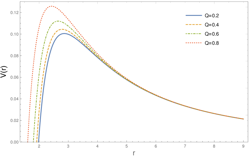
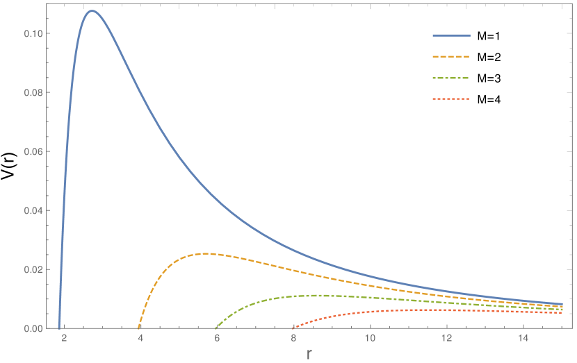
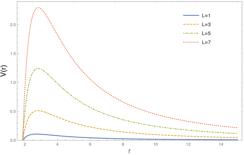
Figure 1: Upper Left: Effective potential $V(r)$ is shown as function of $r$ keeping fixed parameters at $M=1$, $L=1$. Upper Right Effective potential $V(r)$ is shown as function of $r$ keeping fixed parameters at $Q=0.5$, $L=1$ and Lower Centre: Effective potential $V(r)$ is shown as function of $r$ keeping fixed parameters at $M=1$, $Q=0.5$.

2 Formation of Regular BH for Non-Linear electrodynamics

The coupling of Non-linear electrodynamics(NLED) with gravity gives rise to a regular BH for spherically symmetric space-time. Unlike singular BH, the curvature of the space-time does not blow up at $r=0$. The theory of regular BH was first proposed by Bardeen Bardeen . Since then different types of regular black holes have been proposed Mars_1996 ; Barrab ; Borde ; AyonBeato:1998ub ; Ayon-Beato1999 ; Ayon-Beato:2000mjt ; PhysRevLett.96.031103 . The importance of the study of regular BH is that it would give an understanding of the final state of the gravitational collapse.

The action for gravity couple with NLED is written as

$$S(g_{\mu,\nu},A_{\mu})=\int\left[\frac{R}{16\pi}-\frac{1}{4\pi}\mathcal{L}(F)\right]\sqrt{-g}d^{4}x$$ (1)

Where $R$ is the scalar curvature and $F$ is the electromagnetic field scalar defined as $F=\frac{1}{4}F_{\mu\nu}F^{\mu\nu}$,where $F_{\mu\nu}$ is the electromagnetic strength. The action is to be varied with respect to $g_{\mu\nu}$ in order to get Einstein’s equations:

$$R_{\mu\nu}-\frac{1}{2}g_{\mu\nu}R=8\pi T_{\mu\nu}$$ (2)

where $R_{\mu\nu}$ is the Ricci tensor and $T_{\mu\nu}$ is energy-momentum tensor defined as

$$T_{\mu\nu}=\mathcal{L}(F)g_{\mu\nu}-\dfrac{d\mathcal{L}(F)}{dF}F_{\mu\sigma}F_{\nu}^{\sigma}$$ (3)

In order to solve the Einstein’s equation coupled with NLED, we here assume AyonBeato:1999rg ; Berej:2006cc

$$\mathcal{L}(F)=F\left[1-\tanh^{2}\left(\frac{|Q|}{2M}(2Q^{2}F)^{\frac{1}{4}}\right)\right]$$ (4)

where $Q$ and $M$ are the charge and mass of the BH respectively. The solution of Einstein’s equation then gives rise to static spherically symmetric metric described as

$$ds^{2}=-f(r)dt^{2}+\frac{1}{f(r)}dr^{2}+r^{2}d\Omega^{2}$$ (5)

where

$$f(r)=1-\frac{2M}{r}+\frac{2M}{r}\tanh\left(\frac{Q^{2}}{2Mr}\right)$$ (6)

This metric is asymptotically flat, and reduces to Reissner-Nordström metric for smaller value of $Q$. This metric corresponds to a charged BH,does not possess any singularity inside or on the event horizon, only if the value of charge of the source lies below $1.05M$ i.e. $\left|Q\right|\leq 1.05M$ AyonBeato:1999rg . The coupling of Non-linear electrodynamics (NLED) for a specific Lagrangian $\mathcal{L}(F)$ (see Eq-(4)) with gravity gives rise to the Ayon-Beato Garcia Regular Black Holes. Using FP duality the metric function Eq-(6) can be reproduced within a different formulation namely by using $\mathcal{L}(F)=\frac{F}{\cosh^{2}\left(a|F/2|^{\frac{1}{4}}\right)}$, where ‘$a$’ is a constant PhysRevD.63.044005 .

3 Dynamical Evolution of Perturbation

The perturbation of BHs can be achieved in two ways: Either one can add field to the BH space-time or perturb the BH metric itself. The later one means that massive celestial objects disturb the BH space-time i.e. gravitational perturbation. In this paper, we add scalar field to the BH background and see how it couples with gravity of the BH. The Lagrangian of the minimal coupling of a perturbation of a scalar field with gravity is given by

$$L_{MC}=\frac{1}{2}\nabla_{\nu}\Phi\nabla^{\nu}\Phi-\frac{1}{2}\mu^{2}\Phi^{2}$$ (7)

If this scalar field does not backreact on the BH background, then the equation of motion(EOM) of the scalar field in the BH background would be

$$(\nabla_{\nu}\nabla^{\nu}-\mu^{2})\Phi=0$$ (8)

where $\nabla_{\nu}$ is the covariant derivative and $\mu$ is the mass of the scalar field. The metric of static scalar BH is given by

$$d{s}^{2}=-f(r)dt^{2}+\frac{1}{f(r)}dr^{2}+r^{2}d\Omega^{2}$$ (9)

If the background of the BH is static and spherically symmetric, one can use separation of variable method to reduce the above equation into a one dimensional Schrödinger-like equation. For static spherical symmetric background, we can take $\Phi$ as

$$\Phi(t,r,\theta,\phi)=e^{-i\omega t}Y^{m}_{L}(\theta,\phi)\frac{\Psi(r)}{r}$$ (10)

where $Y^{m}_{L}$ are the spherical harmonics. Now the Eq-(8) simplifies to

$$\dfrac{d^{2}\Psi}{dr_{*}^{2}}+[\omega^{2}-V(r)]\Psi=0$$ (11)

where $r_{*}$ is the tortoise coordinate and $V(r)$ is the potential given by

$$V(r)=f(r)\left(\frac{L(L+1)}{r^{2}}+\frac{1}{r}\dfrac{df}{dr}+\mu^{2}\right)$$ (12)

where $L$ is the multipole number.

To solve the Eq-(11), one has to provide the boundary conditions on $\Psi$ at event horizon and spacial infinity. Since no signal come out from an event horizon and no wave coming from infinity to further excite the BH, the choice of boundary conditions such that waves are outgoing at both the boundary 1972ApJ…178..347B . Mathematically

$$\Psi=\begin{cases}e^{-i\omega r_{*}}&\text{if }\hskip 8.53581ptr_{*}\to-\infty\\ e^{+i\omega r_{*}}&\text{if }\hskip 8.53581ptr_{*}\to+\infty\end{cases}$$ (13)

The behaviour of the effective potential is shown in Fig-1. The leftmost figure shows how effective potential depends on the charge of the BH $(Q)$. The height of the potential is increased as the charge of BH is increased. The middle figure shows how effectively potential changes when the mass of the BH $(M)$ is varied. The rightmost figure shows the change in potential when the spherical harmonics no $L$ is varied. This figure clearly shows that the height of the figure is increased as the spherical harmonics no is increased.

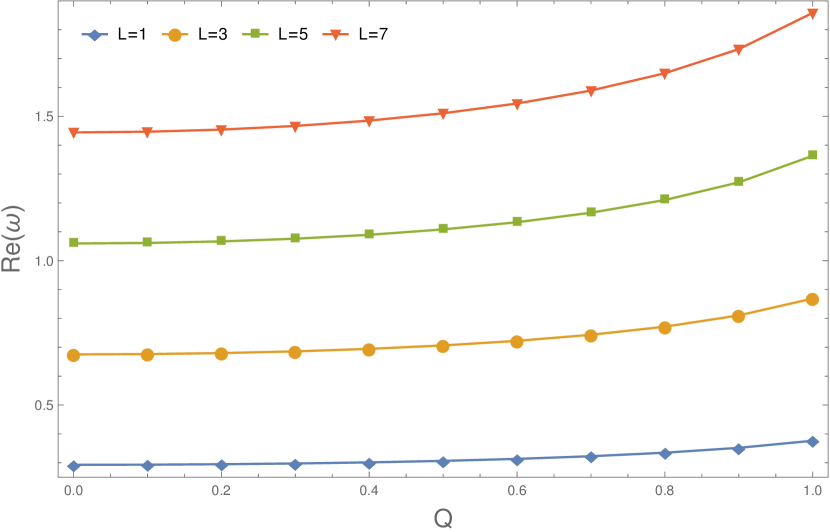
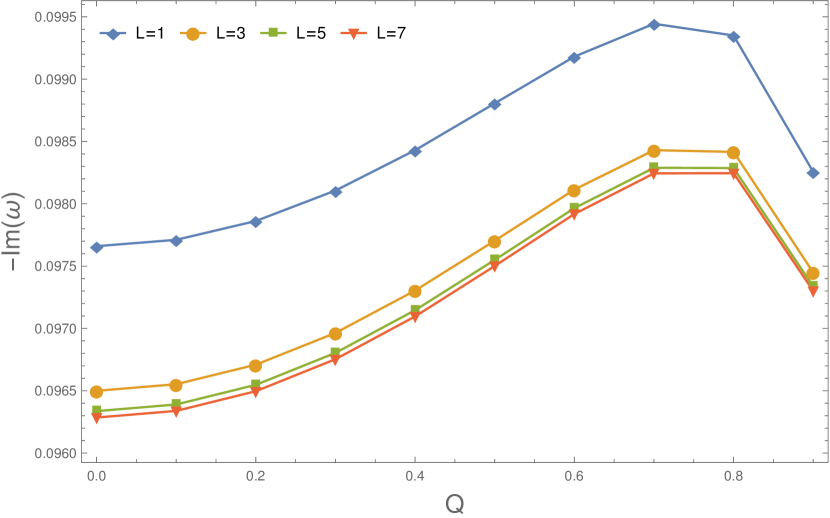
Figure 2: Left: Real part of QNMs [$Re(\omega)$] are shown as function of Charge ($Q$) of keeping fixed parameters at $M=1$, $n=0$ and Right: Imaginary part of QNMs [$-Im(\omega)$] are shown as function of Charge ($Q$) of keeping fixed parameters at $M=1$, $n=0$

.

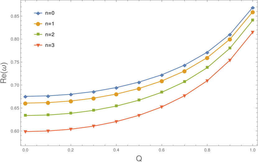
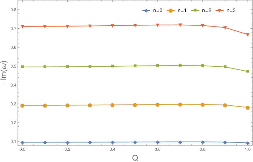
Figure 3: Left: Real part of QNMs [$Re(\omega)$] are shown as function of Charge ($Q$) of keeping fixed parameters at $M=1$, $L=3$ and Right: Imaginary part of QNMs [$-Im(\omega)$] are shown as function of Charge ($Q$) of keeping fixed parameters at $M=1$, $L=3$.

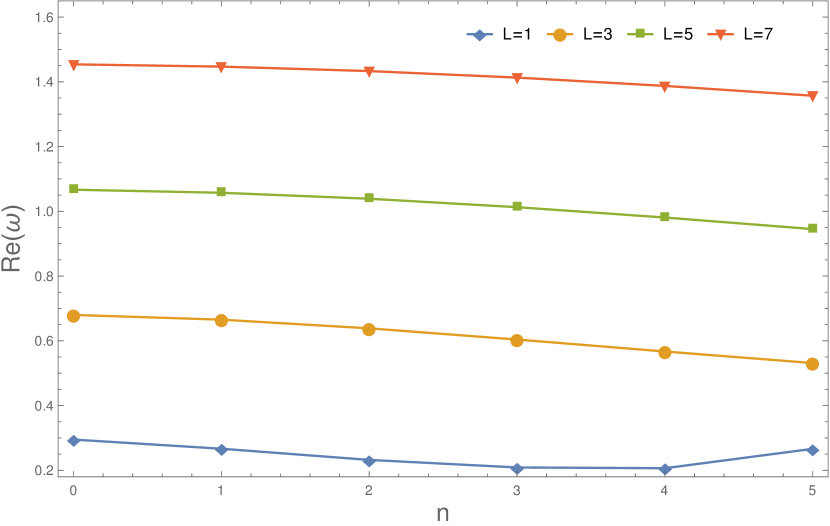
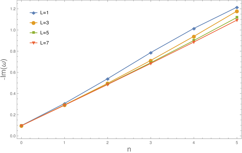
Figure 4: Left: Real part of QNMs [$Re(\omega)$] are shown as function of mode number ($n$) of keeping fixed parameters at $M=1$, $Q=0.2$ and Right: Imaginary part of QNMs [$-Im(\omega)$] are shown as function of mode number ($n$) of keeping fixed parameters at $M=1$, $Q=0.2$.

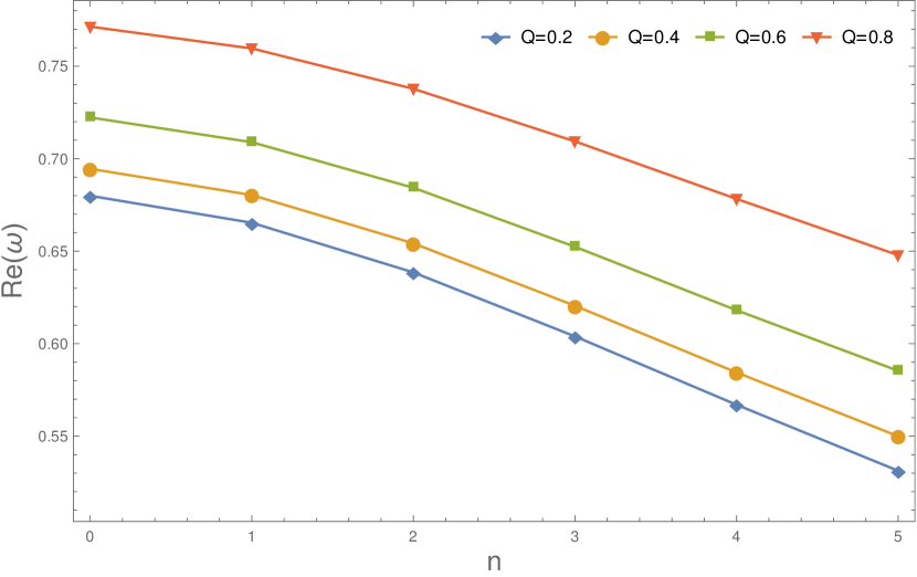
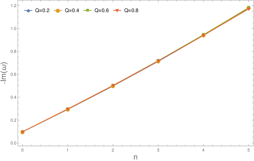
Figure 5: Left: Real part of QNMs [$Re(\omega)$] are shown as function of mode number ($n$) of keeping fixed parameters at $M=1$, $L=3$ and Right: Imaginary part of QNMs [$-Im(\omega)$] are shown as as function of mode number ($n$) of keeping fixed parameters at $M=1$, $L=3$.

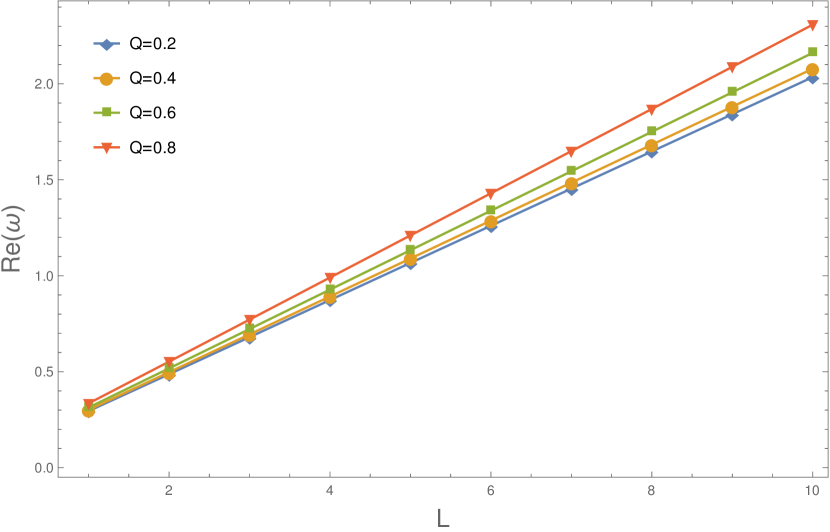
Figure 6: Left: Real part of QNMs [$Re(\omega)$] are shown as function of multipole number $(L)$ of keeping fixed parameters at $M=1$, $n=0$ and Right: Imaginary part of QNMs [$-Im(\omega)$] are shown as function multipole number ($L$) of keeping fixed parameters at $M=1$, $n=0$.

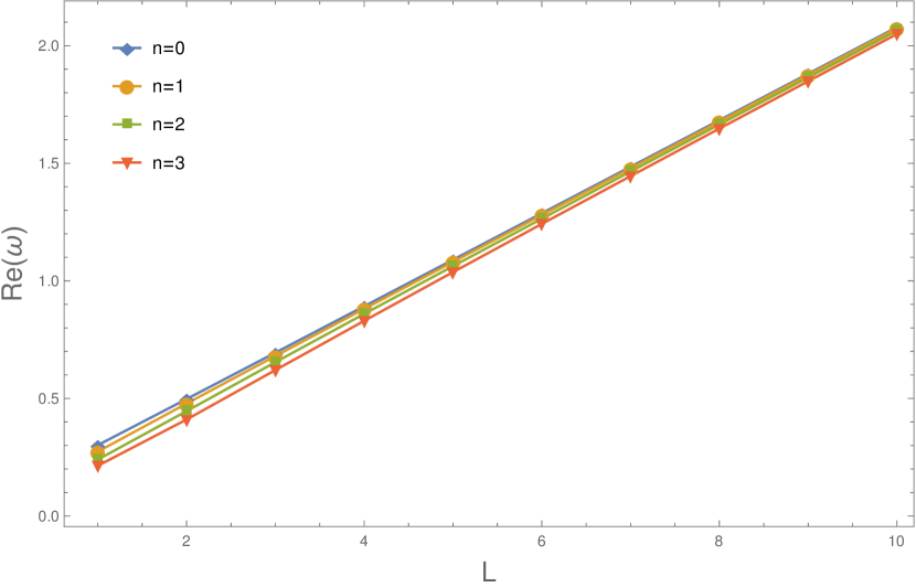
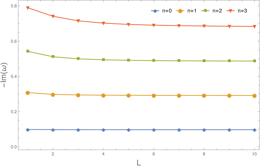
Figure 7: Left: Real part of QNMs [$Re(\omega)$] are shown as function of multipole number $(L)$ of keeping fixed parameters at $M=1$, $Q=0.4$ and Right: Imaginary part of QNMs [$-Im(\omega)$] are shown as function multipole number ($L$) of keeping fixed parameters at $M=1$, $Q=0.4$.

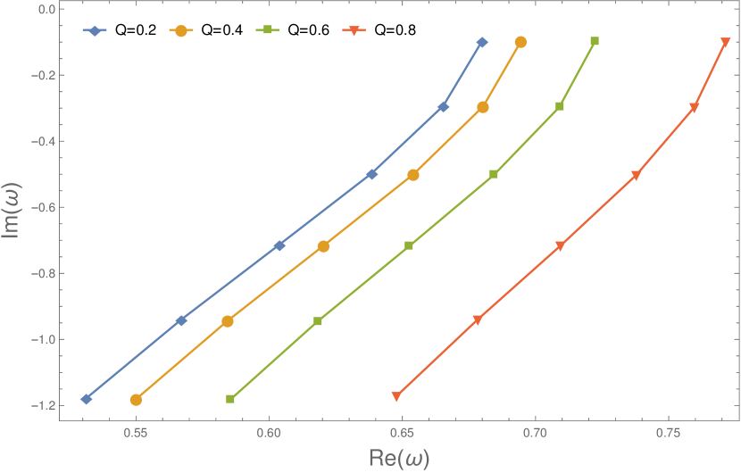
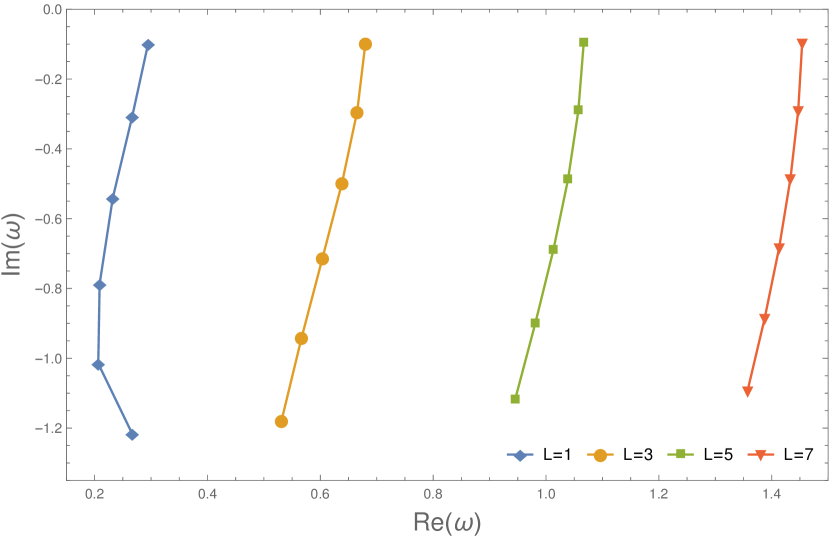
Figure 8: Left: The QNMs are plotted by keeping fixed multiploe number at $L=3$ and Right: The QNMs are plotted by keeping fixed Charge of the BH at $Q=0.2$.

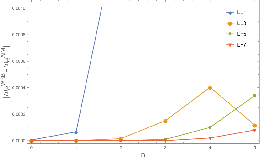
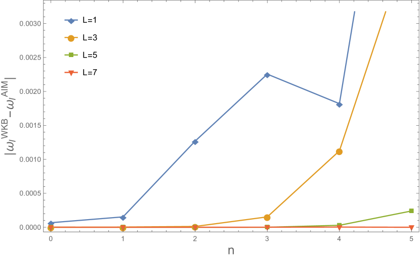
Figure 9: Left: The absolute difference between real part of frequency calculated using WKB and AIM $|\omega^{WKB}_{R}-\omega^{AIM}_{R}|$ vs overtone numbers $n$ and Right: The absolute difference between imaginary part of frequency calculated using WKB and AIM $|\omega^{WKB}_{I}-\omega^{AIM}_{I}|$ vs overtone numbers $n$.

L	n	WKB		AIM
		Re($\omega$)	Im($\omega$)	Re($\omega$)	Im($\omega$)
1	0	0.294919	- 0.0979588	0.294943	- 0.0978619
	1	0.266699	- 0.306989	0.266672	- 0.306742
	2	0.233486	- 0.542641	0.232042	- 0.540594
	3	0.224698	- 0.79528	0.207645	- 0.791114
	4	0.273578	- 1.03941	0.205633	- 1.04657
	5	0.431276	- 1.23769	0.249323	- 1.28677
3	0	0.679946	- 0.0967102	0.679946	- 0.0967092
	1	0.665366	- 0.292893	0.665367	- 0.292890
	2	0.6385	- 0.496942	0.638532	- 0.496939
	3	0.603618	- 0.712533	0.603940	- 0.712370
	4	0.565934	- 0.941304	0.567013	- 0.939842
	5	0.530658	- 1.18319	0.531917	- 1.17717
5	0	1.06679	- 0.0965476	1.06679	- 0.0965476
	1	1.05729	- 0.290777	1.05729	- 0.290777
	2	1.03889	- 0.48835	1.03889	- 0.488351
	3	1.01277	- 0.691261	1.01281	- 0.691269
	4	0.980636	- 0.901104	0.980819	- 0.901093
	5	0.944502	- 1.11895	0.945138	- 1.11868
7	0	1.45398	- 0.0964964	1.45398	- 0.0964964
	1	1.44697	- 0.290102	1.44697	- 0.290102
	2	1.43317	- 0.485529	1.43317	- 0.485529
	3	1.41307	- 0.68393	1.41307	- 0.683934
	4	1.38735	- 0.886353	1.38738	- 0.886365
	5	1.35692	- 1.09368	1.35705	- 1.09369

Table 1: QNMs for the charge of BH $Q=0.2$

L	n	WKB		AIM
		Re($\omega$)	Im($\omega$)	Re($\omega$)	Im($\omega$)
1	0	0.301323	- 0.0985138	0.301339	- 0.0984298
	1	0.273836	- 0.308251	0.273795	- 0.308049
	2	0.241438	- 0.543728	0.239921	- 0.542018
	3	0.233044	- 0.795056	0.214119	- 0.790638
	4	0.281659	- 1.03594	0.160085	-1.01101
	5	0.43885	- 1.22736	0.211545	- 1.11220
3	0	0.694544	- 0.0973048	0.694544	- 0.0973038
	1	0.680351	- 0.294599	0.680351	- 0.294596
	2	0.654201	- 0.499524	0.654227	- 0.499518
	3	0.620254	- 0.715626	0.620513	- 0.715466
	4	0.583612	- 0.944447	0.584460	- 0.943116
	5	0.549413	- 1.18581	0.550303	- 1.18070
5	0	1.08966	- 0.0971462	1.08966	- 0.0971461
	1	1.08041	- 0.292541	1.08041	- 0.292541
	2	1.0625	- 0.491183	1.06250	- 0.491184
	3	1.03708	- 0.695004	1.03711	- 0.695010
	4	1.00581	- 0.905542	1.00596	- 0.905524
	5	0.970648	- 1.12382	0.971179	- 1.12357
7	0	1.48514	- 0.0970962	1.48514	- 0.0970962
	1	1.47831	- 0.291884	1.47831	- 0.291884
	2	1.46488	- 0.488442	1.46488	- 0.488443
	3	1.44531	-0.687889	1.44531	- 0.687892
	4	1.42028	-0.891236	1.42031	- 0.891245
	5	1.39067	- 1.09933	1.39078	- 1.09934

Table 2: QNMs for the charge of BH $Q=0.4$

L	n	WKB		AIM
		Re($\omega$)	Im($\omega$)	Re($\omega$)	Im($\omega$)
1	0	0.313485	- 0.0992476	0.313490	- 0.0991805
	1	0.287529	- 0.309618	0.287462	- 0.309465
	2	0.256777	- 0.543962	0.255072	- 0.542693
	3	0.248881	- 0.792229	0.229728	-0.789974
	4	0.295928	- 1.02734	0.205885	-1.02916
	5	0.449067	- 1.20807	0.182760	- 1.19983
3	0	0.722304	- 0.098115	0.722304	- 0.0981139
	1	0.70892	- 0.296861	0.708920	- 0.296858
	2	0.684259	- 0.502743	0.684274	-0.502731
	3	0.652232	- 0.719043	0.652383	- 0.718890
	4	0.617682	- 0.947138	0.618085	- 0.946013
	5	0.585559	- 1.18668	0.585442	-1.18236
5	0	1.13315	- 0.0979651	1.13315	- 0.0979650
	1	1.12443	-0.29493	1.12443	- 0.294930
	2	1.10755	- 0.494937	1.10755	- 0.494937
	3	1.08358	- 0.699785	1.08359	- 0.699785
	4	1.05408	- 0.9109	1.05418	- 0.910871
	5	1.02092	- 1.12922	1.02126	- 1.12898
7	0	1.5444	-0.097918	1.54440	- 0.0979179
	1	1.53796	- 0.294313	1.53796	- 0.294313
	2	1.52529	- 0.492368	1.52529	- 0.492368
	3	1.50684	-0.693127	1.50684	- 0.693128
	4	1.48324	-0.897532	1.48326	- 0.897535
	5	1.45531	- 1.10637	1.45539	- 1.10637

Table 3: QNMs for the charge of BH $Q=0.6$

L	n	WKB		AIM
		Re($\omega$)	Im($\omega$)	Re($\omega$)	Im($\omega$)
1	0	0.33491	- 0.0994018	0.334902	- 0.0993503
	1	0.311883	- 0.308354	0.311771	- 0.308232
	2	0.283847	- 0.53781	0.281917	- 0.537101
	3	0.275118	- 0.778527	0.257058	-0.778120
	4	0.314347	- 1.00449	0.241982	-1.02535
	5	0.447416	- 1.17416	0.225627	- 1.26343
3	0	0.771405	- 0.0984174	0.771405	- 0.0984163
	1	0.759602	- 0.297409	0.759601	- 0.297404
	2	0.737804	- 0.502491	0.737805	-0.502472
	3	0.709354	- 0.716443	0.709365	- 0.716304
	4	0.678459	- 0.940391	0.678290	- 0.939600
	5	0.649543	- 1.17386	0.647944	-1.17118
5	0	1.21013	- 0.0982866	1.21013	- 0.0982865
	1	1.20244	-0.295747	1.20244	- 0.295747
	2	1.18754	- 0.495812	1.18755	- 0.495811
	3	1.16637	- 0.700008	1.16638	- 0.700002
	4	1.14025	- 0.909541	1.14028	- 0.909500
	5	1.11078	- 1.1252	1.11086	- 1.12499
7	0	1.64928	-0.0982455	1.64928	- 0.0982455
	1	1.6436	- 0.295216	1.64360	- 0.295216
	2	1.63244	- 0.49361	1.63244	- 0.493609
	3	1.61616	-0.694316	1.61616	- 0.694315
	4	1.59532	-0.898132	1.59532	- 0.898129
	5	1.57062	- 1.10573	1.57064	- 1.10571

Table 4: QNMs for the charge of BH $Q=0.8$

4 Methods of Calculations of QNMs

4.1 WKB Approximation

The solution of the Schrödinger-like equation(11) can be achieved by both fully numerical and semi-analytical method based on the problem under consideration. Mashhoon Mashh suggested that the WKB could be used to compute QNMs. WKB technique was first developed by Schutz and Will Schutz:1985 to solve a problem of scattering around BHs. Iyer and Will Iyer-I in their paper extended this method to third order and Konoplya PhysRevD.68.124017 ; Konoplya:2004ip extended this to sixth order. This method allows us to study the QNMs of BH systemically and is applied to any BHs problem with boundary conditions given by Eq-(13). In this method, we match two asymptotic wave function near the position of maximized potential. The QNMs are to be calculated using the WKB method of sixth-order by a formula given by

$$\frac{i(\omega^{2}-V_{o})}{\sqrt{-2V^{{}^{\prime\prime}}_{o}}}-\sum_{j=2}^{6}\Lambda_{j}=n+\frac{1}{2}$$ (14)

where $V_{o}$ is the maximized potential and $V^{{}^{\prime\prime}}_{o}$ is the second-order potential w.r.t tortoise coordinate at the position of maximized potential and $\Lambda_{j}$ is the jth order correction term of the WKB approximation. These correction terms $\Lambda_{2}$,$\Lambda_{3}$ and $\Lambda_{4}$,$\Lambda_{5}$,$\Lambda_{6}$ can be found in Iyer-II and PhysRevD.68.024018 respectively.

4.2 The Asymptotic Iteration Method(AIM)

First we consider a second order homogeneous differential equation for the function $\Psi$ as

$$\dfrac{d^{2}\Psi(x)}{dx^{2}}=\lambda_{o}(x)\dfrac{d\Psi(x)}{dx}+s_{o}(x)\Psi(x)$$ (15)

where $\lambda_{o}(x)$ and $s_{o}(x)$ are the continuous function in between the points a and b. The above equation can be taken derivative upto $(n+1)$th and $(n+2)$th order, where $n=1,2,3,...$. Therefore we have

$$\dfrac{d^{n+1}\Psi(x)}{dx^{n+1}} =\lambda_{n-1}(x)\dfrac{d\Psi(x)}{dx}+s_{n-1}(x)\Psi(x)$$ (16a)

$$\dfrac{d^{n+2}\Psi(x)}{dx^{n+2}} =\lambda_{n}(x)\dfrac{d\Psi(x)}{dx}+s_{n}(x)\Psi(x)$$ (16b)

where

$$\lambda_{n}(x) =\frac{d\lambda_{n-1}(x)}{dx}+s_{n-1}(x)+\lambda_{0}(x)\lambda_{n-1}(x)$$ (17a)

$$s_{n}(x) =\dfrac{ds_{n-1}(x)}{dx}+s_{o}(x)\lambda_{n-1}(x)$$ (17b)

these two recurrence relations was first found by Ciftci Ciftci_2003 ; article .

We introduce the asymptotic aspect of the method by choosing the sufficient large value of n. Therefore we have

$$\frac{s_{n}(x)}{\lambda_{n}(x)}=\frac{s_{n-1}(x)}{\lambda_{n-1}(x)}\equiv\alpha(x)$$ (18)

and the quantization condition is given by

$$\Delta_{n}=s_{n}\lambda_{n-1}-s_{n-1}\lambda_{n}\hskip 8.53581pt\text{n=1,2,3,..}$$ (19)

The solution of the equation then can be written as

$$\Psi(x)=\exp{\left(\int^{x}\alpha(y)dy\right)}*\\ \left[C_{2}+C_{1}\int^{x}\exp{\left\{{\int^{y}\left(\lambda_{o}(z)+2\alpha(z)\right)dz}\right\}dy}\right]$$ (20)

where $C_{1}$ and $C_{2}$ are two constants.

4.2.1 The Improved AIM

Since the above two recurrence relations involves derivative of the previous iteration, it takes lots of time to calculate these recurrence relations, time increases exponentially as no of iteration increase. In the following improved version of AIM, all the derivatives are excluded at each step to make this method time-efficient Cho_2010 . To do the aforesaid, $\lambda_{n}$ and $s_{n}$ are expanded in a Taylor series around the point at which one wants to perform the AIM, $x_{m}$

$$\lambda_{n}(x_{m}) =\sum_{i=o}^{\infty}c_{n}^{i}(x-x_{m})^{i}$$ (21a)

$$s_{n}(x_{m}) =\sum_{i=0}^{\infty}d_{n}^{i}(x-x_{m})^{i}$$ (21b)

where $c_{n}^{i}$ and $d_{n}^{i}$ are the ith Taylor coefficient of $\lambda_{n}(x_{m}$ and $s_{n}(x_{m})$ respectively. Now we substitute the above expression into the previous set of recursion relation to get new set of recursion relation for the coefficient

$$c_{n}^{i} =(i+1)c_{n+1}^{i+1}+d_{n-1}^{i}+\sum_{k=0}^{i}c_{0}^{k}c_{n-1}^{i-k}$$ (22a)

$$d_{n}^{i} =(i+1)d_{n-1}^{i+1}+\sum_{k=0}^{i}d_{0}^{k}c_{n-1}^{i-k}$$ (22b)

These recursion relations do not involve any derivative operators. The quantization condition for this improved method is given by

$$d_{n}^{0}c_{n-1}^{0}-d_{n-1}^{0}c_{n}^{0}=0$$ (23)

The reason behind of the choosing such quantization was explained in Cho_2010

5 Calculation of the QNMS using AIM

We first do a coordinate transformation to make the radial equation relevant to AIM which leads to a simpler solution. For the ABG BH, it is convenient to change coordinate $r$ to $x$ as $x=\frac{1}{r}$. The radial equation then can be written in terms of $x$ as

$$\dfrac{d^{2}\Psi}{dx^{2}}+\dfrac{d[ln(x^{2}f)]}{dx}\dfrac{d\Psi}{dx}+\left(\frac{\omega^{2}}{x^{4}f^{2}}-\frac{L(L+1)x^{2}}{f}+\frac{1}{xf}\dfrac{df}{dx}\right)\Psi=0$$ (24)

Since only the outgoing waves survive at the boundary and there is a regular singularity at the event horizon,we define $\Psi$ as

$$\Psi=(x-x_{o})^{-\frac{i\omega}{K_{o}}}e^{-i\omega\int\frac{dx}{x^{2}f(x)}}u(x)$$ (25)

where $x_{o}$ is the position of the event horizon and $K_{o}$ is the surface gravity at horizon defined as

$$K_{o}=\left.\frac{1}{2}\dfrac{df}{dr}\right|_{r\to r_{o}}=\left.-\frac{x^{2}}{2}\dfrac{df}{dx}\right|_{x\to x_{o}}$$ (26)

The Eq-(24) then takes form

$$\dfrac{d^{2}u(x)}{dx^{2}}=\lambda_{o}(x)\dfrac{du(x)}{dx}+s_{o}(x)u(x)$$ (27)

with

$$\lambda_{o}=\frac{-x^{2}\left\{3M\sinh\left(\frac{Q^{2}x}{M}\right)+Q^{2}x\right\}\text{sech}^{2}\left(\frac{Q^{2}x}{2M}\right)+6Mx^{2}-2x+2i\omega}{x^{2}\left\{2Mx\tanh\left(\frac{Q^{2}x}{2M}\right)-2Mx+1\right\}}+\frac{2i\omega}{(x-x_{o})K_{o}}$$ (28)

$$s_{o}=\frac{1}{x^{2}(x-x_{o})^{2}K_{o}^{2}\left(2Mx\tanh\left(\frac{Q^{2}x}{2M}\right)-2Mx+1\right)}\left[x^{2}\omega^{2}\left\{2Mx\tanh\left(\frac{Q^{2}x}{2M}\right)-2Mx+1\right\}\right.\\ \left.+i\omega K_{o}\left\{x^{2}\left\{2M(2x-3x_{o})\tanh\left(\frac{Q^{2}x}{2M}\right)+Q^{2}x(x-x_{o})\text{sech}^{2}\left(\frac{Q^{2}x}{2M}\right)\right\}-4Mx^{3}+x^{2}(6Mx_{o}+1)-2x(x_{o}+i\omega)+2ix_{o}\omega\right\}\right.\\ \\ +\left.\frac{1}{2}(x-x_{o})^{2}K_{o}^{2}\text{sech}^{2}\left(\frac{Q^{2}x}{2M}\right)\left\{\left(L^{2}+L+2Mx\right)\cosh\left(\frac{Q^{2}x}{M}\right)+L^{2}+L+2x\left(M-Q^{2}x\right)-2Mx\sinh\left(\frac{Q^{2}x}{M}\right)\right\}\right]$$ (29)

To calculate QNMs using AIM, we first find the event horizon in term of $x$ by expanding $f(x)$ about $x=0$ and kept up to 50 terms, then we equate with expanded $f(x)$ to zero to get the event horizon. After finding the value of $\lambda_{o}$ and $s_{o}$, we expand $\lambda_{o}$ and $s_{o}$ in Taylor series about the point where the effective potential get maximized. The ith components of the Taylor series of $\lambda_{o}$ and $s_{o}$ are identified as $c_{0}^{i}$ and $d_{0}^{i}$ respectively. Then using the recurrence relation Eq-(22), we find other $c_{n}^{i}$ and $d_{n}^{i}$. At some large value of n, we truncate the iteration. Then we solve the Eq-(23) to find the QNMs frequency. We use Mathematica Software to perform all the calculations.

6 conclusion

We calculate QNMs of ABG regular BH for the scalar field using two methods WKB and AIM. We show the calculated numerical values of QNMs in table 1-4. The calculation shows that the difference between WKB and AIM significantly reduces as the multipole number increases (see Fig-9). WKB method works correctly for $n\leq L$ .For lower multipole number and higher mode, the calculated QNMs using AIM is more acceptable than WKB.

The Fig-2 and Fig-3 show that the real part of QNMs frequency monotonically increases but the imaginary part first increases and gets maximized around $Q=0.7$ then decreases rapidly (Fig-2) as the value of $Q$ increases. The Fig-4 and Fig-5 show that the real part of frequency decreases and imaginary part linearly increases as the mode number ($n$) increases. The Fig-6 and Fig-7 show that the real part of frequency approximately linear with multipole number ($L$) and the imaginary part is greatest for the lower value of multipole number ($L$).We see the imaginary part gets independent of multipole number ($L$) for larger multipole number ($L$) which reflects the effect of the eikonal limit i.e. $L\to\infty$ . Therefore, the stability of ABG BH is highest around the charge of the BH $Q=0.7$ against the scalar field for BH mass $M=1$. All the QNMs are found stable. How the real and imaginary part of QNMs is related to each other is shown in Fig-8

The QNMs of different regular charged BH for the massless scalar field was studied in PhysRevD.87.024034 . Our result is consistent in comparison to the findings of PhysRevD.87.024034 and reproduces known results in the Schwarzschild limit.We extend the works of the authors of PhysRevD.87.024034 for a particular metric given by references [4,5] in PhysRevD.87.024034 by studying how QNMs are dependent on the BH parameters in details and also find the heights possible region of charge of BH for which BH is most stable.

Note

Before the acceptance of our paper, we were unaware that our work is closely related to these refId0 ; Li:2016oif ; Lopez:2018aec ; Panotopoulos:2019qjk ; PhysRevD.103.124050 ; Cai:2020kue works. Although, the lapse function of our ABG BH is different from the lapse function of the ABG BHs used by many authors to compute their QNMs. No authors have studied the QNMs of the ABG BH having this same lapse function in detail as we have done in our paper.

References

- (1) J Maldacena Int.J.Theor.Phys. 38, 1113(1999)
- (2) G T Horowitz and V E Hubeny Phys. Rev. D 62, 024027(2000)
- (3) J D Bekenstein and V Mukhanov Phys. Lett. B 360, 7(1995)
- (4) S Hod Phys. Rev. Lett. 81, 4293(1998)
- (5) O Dreyer Phys. Rev. Lett. 90, 081301(2003)
- (6) T Regge and J A Wheeler Phys. Rev. 108, 1063(1957)
- (7) F J Zerilli Phys. Rev. D 2, 2141(1970)
- (8) F J Zerilli Phys. Rev. Lett. 24, 737(1970)
- (9) C V Vishveshwara Phys. Rev. D 1, 2870(1970)
- (10) C V Vishveshwara Nature 227, 936(1970)
- (11) S Chandrasekhar and S L Detweiler Proc. Roy. Soc. Lond. A344, 441(1975)
- (12) H J Blome and B Mashhoon Phys. Lett. A 100, 231(1984)
- (13) V Ferrari and B Mashhoon Phys. Rev. D 30, 295(1984)
- (14) E W Leaver J. Math. Phys. 27, 1238(1986)
- (15) E W Leaver Phys. Rev. D 34, 384(1986)
- (16) E W Leaver Proc. Roy. Soc. Lond. A402, 285(1985)
- (17) G T Horowitz and V E Hubeny Phys. Rev. D 62, 024027(2000)
- (18) H T Cho, A S Cornell, J Doukas, and W Naylor Class. Quant. Grav. 27, 155004(2010)
- (19) H P Nollert Class. Quant. Grav. 16, 159(1999)
- (20) K D Kokkotas and B G Schmidt Living Rev. Relativ 2, 2(1999)
- (21) E Berti, V Cardoso, and A O Starinets Class. Quant. Grav. 26, 163001(2009)
- (22) R A Konoplya and A Zhidenko Rev. Mod. Phys. 83, 793(2011)
- (23) J Bardeen published in the conference proceeding in the U.S.S.R (1968)
- (24) M Mars, M M Martín-Prats, and J M M Senovilla Class. Quant. Grav. 13, 51(1996)
- (25) C Barrabès and V P Frolov Phys. Rev. D 53, 3215(1996)
- (26) A Borde Phys. Rev. D 50, 3692(1994)
- (27) E Ayon-Beato and A Garcia Phys. Rev. Lett. 80, 5056(1998)
- (28) E Ayon-Beato and A Garcia Gen. Relativ. Gravit. 31, 629(1999)
- (29) E Ayon-Beato and A Garcia Phys. Lett. B 493, 149(2000)
- (30) S A Hayward Phys. Rev. Lett. 96, 031103(2006)
- (31) A Flachi and J P S Lemos Phys. Rev. D 87, 024034(2013)
- (32) B Toshmatov, A Abdujabbarov, Z Stuchlík, and B Ahmedov Phys. Rev. D 91, 083008(2015)
- (33) B Toshmatov, Z Stuchlík, and B Ahmedov Phys. Rev. D 98, 085021(2018)
- (34) C Wu Eur. Phys. J. C 78, 283(2018)
- (35) J Li, K Lin, and H Wen Adv. High Energy Phys. 2017, 5234214(2017)
- (36) L A Lopez and V Hinojosa Can. J. Phys. 99(1), 44(2020)
- (37) G Panotopoulos and A Rincón Eur. Phys. J. Plus 134, 300(2019)
- (38) X C Cai and Y G Miao Phys. Rev. D 103, 124050(2021)
- (39) S H Hendi, S N Sajadi, and M Khademi Phys. Rev. D 103, 064016(2021)
- (40) X C Cai and Y G Miao Phys. Rev. D 102, 084061(2020)
- (41) K A Bronnikov, R A Konoplya and A Zhidenko Phys. Rev. D 86, 024028(2012)
- (42) M S Churilova and Z Stuchlik Class. Quant. Grav. 37, 075014(2020)
- (43) K A Bronnikov and R A Konoplya Phys. Rev. D 101, 064004(2020)
- (44) E Ayon-Beato and A Garcia Phys. Lett. B 464, 25(1999)
- (45) W Berej, J Matyjasek, D Tryniecki and M Woronowicz Gen. Rel. Grav. 38, 885(2006)
- (46) K A Bronnikov Phys. Rev. D 63, 044005(2001)
- (47) J M Bardeen, W H Press, and S A Teukolsky Astrophys. J 178, 347(1972)
- (48) B. Mashhoon Proc. 3rd Marcel Grossmann Meeting on Recent Developments of General Relativity ed H Ning (Amsterdam: North-Holland), (1983)
- (49) B F Schutz and C M Will Astrophys. J 291, 33(1985)
- (50) S Iyer and C M Will Phys. Rev. D 35, 3621(1987)
- (51) R A Konoplya Phys. Rev. D 68, 124017(2003)
- (52) R A Konoplya J. Phys. Stud. 8, 93(2004)
- (53) S Iyer Phys. Rev. D 35, 3632(1987)
- (54) R A Konoplya Phys. Rev. D 68, 024018(2003)
- (55) H Ciftci, R L Hall and N Saad J. Phys. Math. Gen. 36, 11807(2003)
- (56) H Ciftci, R Hall and N Saad Phys. Lett. A 340, 388(2005)