1 Introduction

Federated learning is a newly emerging paradigm for machine learning where multiple data holders (clients) collaborate to train a model on their combined dataset. Clients only share partially trained models and other statistics computed from their dataset, keeping their raw data local and private (McMahan et al., 2017; Kairouz et al., 2021). By obviating the need for a third party to collect and store clients’ data, federated learning has several advantages over the classical, centralized paradigm (Dean et al., 2012; Iandola et al., 2016; Goyal et al., 2017): it ensures clients’ consent is tied to the specific task at hand by requiring active participation of the clients in training, confers some basic level of privacy, and has the potential to make machine learning more participatory in general (Kulynych et al., 2020; Jones and Tonetti, 2020). Further, widespread legislation of data portability and privacy requirements (such as GDPR and CCPA) might even make federated learning a necessity (Pentland et al., 2021).

Collaboration among clients is most attractive when clients have very different subsets of the combined dataset (data heterogeneity). For example, different autonomous driving companies may only be able to collect data in weather conditions specific to their location, whereas their vehicles would need to function under all conditions. In such a scenario, it would be mutually beneficial for companies in geographically diverse locations to collaborate and share data with each other. Further, in such settings, clients are physically separated and connected by ad-hoc networks with large latencies and limited bandwidth. This is especially true when clients are edge devices such as mobile phones, IoT sensors, etc. Thus, communication efficiency is crucial for practical federated learning. However, it is precisely under such circumstances (large data heterogeneity and low communication) that current algorithms fail dramatically (Hsieh et al., 2020; Li et al., 2020; Karimireddy et al., 2020b; Reddi et al., 2021; Wang et al., 2020b; Acar et al., 2021; Li et al., 2021b; Afonin and Karimireddy, 2021; Wang et al., 2021, etc.). This motivates our central question: Why do current federated methods fail in the face of data heterogeneity—and how can we fix them?

Our solution.

We make two main observations: (i) We show that, even with data heterogeneity, linear models can be trained in a federated manner through gradient correction techniques such as SCAFFOLD (Karimireddy et al., 2020b). While this observation is promising, it alone remains limited, as linear models are not rich enough to solve practical problems of interest (e.g., those that require feature learning). (ii) We shed light on why current federated algorithms struggle to train deep, nonconvex models. We observe that the failure of existing methods for neural networks is not uniform across the layers. The early layers of the network do in fact learn useful features, but the final layers fail to make use of them. Specifically, federated optimization applied to this nonconvex problem results in distorted final layers.

These observations suggest a train-convexify-train federated algorithm, which we call TCT: first, use any off-the-shelf federated algorithm (such as FedAvg, McMahan et al., 2017) to train a deep model to extract useful features; then, compute a convex approximation of the deep model using its empirical Neural Tangent Kernel (eNTK) (Jacot et al., 2018; Lee et al., 2019; Fort et al., 2020; Long, 2021; Wei et al., 2022), and use gradient correction methods such as SCAFFOLD to train the final model. Effectively, the second-stage features freeze the features learned in the first stage and fit a linear model over them. We show that this simple strategy is highly performant on a variety of tasks and models—we obtain accuracy gains up to $36$% points on FMNIST with a CNN, $37$% points on CIFAR10 with ResNet18-GN, and $16$% points on CIFAR100 with ResNet18-GN. Further, its convergence remains unaffected even by extreme data heterogeneity. Finally, we show that given a pre-trained model, our method completely closes the gap between centralized and federated methods.

2 Related Work

Federated learning.

There are two main motivating scenarios for federated learning (FL). The first is where internet service companies (e.g., Google, Facebook, Apple, etc.) want to train machine learning models over their users’ data, but do not want to transmit raw personalized data away from user devices (Ramaswamy et al., 2020; Bonawitz et al., 2021). This is the setting of cross-device federated learning and is characterized by an extremely large number of unreliable clients, each of whom has very little data and the collections of data are assumed to be homogeneous (Kairouz et al., 2021; Bonawitz et al., 2019; Karimireddy et al., 2020a; Bonawitz et al., 2021). The second motivating scenario is when valuable data is split across different organizations, each of whom is either protected by privacy regulation or is simply unwilling to share their raw data. Such “data islands” are common among hospital networks, financial institutions, autonomous-vehicle companies, etc. This is known as cross-silo federated learning and is characterized by a few highly reliable clients, who potentially have extremely diverse data. In this work, we focus on the latter scenario.

Metrics in FL.

FL research considers numerous metrics, such as fairness across users (Mohri et al., 2019; Li et al., 2019; Shi et al., 2021), formal security and privacy guarantees (Bonawitz et al., 2017; Ramaswamy et al., 2020; Fung et al., 2018; Mothukuri et al., 2021), robustness to corrupted agents and corrupted training data (Blanchard et al., 2017; So et al., 2020; Fang et al., 2020; Karimireddy et al., 2021; He et al., 2022), preventing backdoors at test time (Bagdasaryan et al., 2020; Sun et al., 2019; Wang et al., 2020a; Lyu et al., 2020), etc. While these concerns are important, the main goal of FL (and our work) is to achieve high accuracy with minimal communication (McMahan et al., 2017). Clients are typically geographically separated yet need to communicate large deep learning models over unoptimized ad-hoc networks (Kairouz et al., 2021). Finally, we focus on the setting where all users are interested in training the same model over the combined dataset. This is in contrast to model-agnostic protocols (Lin et al., 2020; Ozkara et al., 2021; Afonin and Karimireddy, 2021) or personalized federated learning (Deng et al., 2020; Fallah et al., 2020; Wu et al., 2020; Collins et al., 2021; Kulkarni et al., 2020; Chayti and Karimireddy, 2022). Finally, we focus on minimizing the number of rounds required. Our approach can be combined with communication compression, which reduces bits sent per round (Suresh et al., 2017; Alistarh et al., 2017; Haddadpour et al., 2021; Stich and Karimireddy, 2020).

Federated optimization.

Algorithms for FL proceed in rounds. In each round, the server sends a model to the clients, who partially train this model using their local compute and data. The clients send these partially trained models back to the server who then aggregates them, finishing a round. FedAvg (McMahan et al., 2017), which is the de facto standard FL algorithm, uses SGD to perform local updates on the clients and aggregates the client models by simply averaging their parameters. Unfortunately, however, FedAvg has been observed to perform poorly when faced with data heterogeneity across the clients (Hsieh et al., 2020; Li et al., 2020; Karimireddy et al., 2020b; Reddi et al., 2021; Wang et al., 2020b; Acar et al., 2021; Li et al., 2021b; Afonin and Karimireddy, 2021; Wang et al., 2021; du Terrail et al., 2022, etc.). Theoretical investigations of this phenomenon (Karimireddy et al., 2020b; Woodworth et al., 2020) showed that this was a result of gradient heterogeneity across the clients. Consider FedAvg initialized with the globally optimal model. If this model is not also optimal for each of the clients as well, the local updates will push it away from the global optimum. Thus, convergence would require a careful tuning of hyper-parameters. To overcome this issue, SCAFFOLD (Karimireddy et al., 2020b) and FedDyn (Acar et al., 2021) propose to use control variates to correct for the biases of the individual clients akin to variance reduction (Johnson and Zhang, 2013; Defazio et al., 2014). This gradient correction is applied in every local update by the client and provably nullifies the effect of gradient heterogeneity (Karimireddy et al., 2020b; Mishchenko et al., 2022; Chayti and Karimireddy, 2022). However, as we show here, such methods are insufficient to overcome high data heterogeneity especially for deep learning. Other, more heuristic approaches to combat gradient heterogeneity include using a regularizer (Li et al., 2020) and sophisticated server aggregation strategies such as momentum (Hsu et al., 2019; Wang et al., 2019a; Lin et al., 2021) or adaptivity (Reddi et al., 2021; Karimireddy et al., 2020a; Charles et al., 2021).

A second line of work pins the blame on performance loss due to averaging nonconvex models. To overcome this, Singh and Jaggi (2020); Yu et al. (2021) propose to learn a mapping between the weights of the client models before averaging, Afonin and Karimireddy (2021) advocates a functional perspective and replaces the averaging step with knowledge distillation, and Wang et al. (2019b); Li et al. (2021b); Tan et al. (2021) attempt to align the internal representations of the client models. However, averaging is unlikely to be the only culprit since FedAvg does succeed under low heterogeneity, and averaging nonconvex models can lead to improved performance (Izmailov et al., 2018; Wortsman et al., 2022).

Neural Tangent Kernels (NTK) and neural network linearization.

NTK was first proposed to analyze the limiting behavior of infinitely wide networks (Jacot et al., 2018; Lee et al., 2019). While NTK with MSE may be a bad approximation of real-world finite networks in general (Goldblum et al., 2019), it approximates the fine-tuning of a pre-trained network well (Mu et al., 2020), especially with some minor modifications (Achille et al., 2021). That is, NTK cannot capture feature learning but does capture how a model utilizes learnt features better than last/mid layer activations.

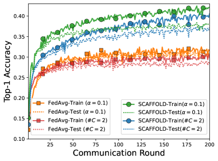
(a) Using linear model.

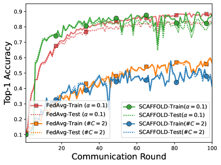
(b) Using ResNet-18.

Figure 1: Performance of FedAvg and SCAFFOLD on CIFAR10 when data are split among ten clients in two ways (#C=2 and $\alpha$=0.1). The #C=2 split is more non-i.i.d. than the $\alpha$=0.1 split. For convex problems (left), gradient correction methods such as SCAFFOLD are relatively unaffected by data heterogeneity, and consistently outperform FedAvg. However, for nonconvex problems (right), FedAvg and SCAFFOLD perform very similarly and both are strongly negatively affected by data heterogeneity.

3 The Effect of Nonconvexity

In this section, we investigate the poor performance of FedAvg (McMahan et al., 2017) and SCAFFOLD (Karimireddy et al., 2020b) empirically in the setting of deep neural networks, focusing on image classification with a ResNet-18. To construct our federated learning setup, we split the CIFAR-10 dataset in a highly heterogeneous manner among ten clients. We either assign each client two classes (denoted by #C=2) or distribute samples according to a Dirichlet distribution with $\alpha=0.1$ (denoted by $\alpha$=0.1). For more details, see Section 5.1.

Insufficiency of gradient correction methods.

Current theoretical work (e.g., Karimireddy et al., 2020b; Reddi et al., 2021; Acar et al., 2021; Wang et al., 2022) attributes the slowdown from data heterogeneity to the individual clients having varying local optima. If no single model is simultaneously optimal for all clients, then the updates of different clients can compete with and distort each other, leading to slow convergence. This tension is captured by the variance of the updates across the clients (client gradient heterogeneity, see Wang et al., 2021). Gradient correction methods such as SCAFFOLD (Karimireddy et al., 2020b) and FedDyn (Acar et al., 2021) explicitly correct for this and are provably unaffected by gradient heterogeneity for both convex and nonconvex losses.

These theoretical predictions are aligned with the results of Figure 1(a), where the loss landscape is convex: SCAFFOLD is relatively unaffected by the level of heterogeneity and consistently outperforms FedAvg. In particular, performance is largely dictated by the algorithm and not the data distributions. This shows that client gradient heterogeneity captures the difficulty of the problem well. On the other hand, when training a ResNet-18 model with nonconvex loss landscape, Figure 1(b) shows that both FedAvg and SCAFFOLD suffer from data heterogeneity. This is despite the theory of gradient correction applying to both convex and nonconvex losses. Further, the train and test accuracies in Figure 1(b) match quite closely, suggesting that the failure lies in optimization (not fitting the training data) rather than generalization. Thus, while the current theory makes no qualitative distinctions between convex and nonconvex convergence, the practical behavior of algorithms in these settings is very different. Such differences between theoretical predictions and practical reality suggests that black-box notions such as gradient heterogeneity are insufficient for capturing the difficulty of training deep models.

Table 1: Feature learning by FedAvg. We report the test accuracy of a ResNet-18 after (centralized) retraining of the last $\ell$ layers on CIFAR10. The earlier $(7-\ell)$ layers are frozen to either random initialization or to the weights of a FedAvg-trained model. The difference measures utility of the $(7-\ell)$ layers learnt by FedAvg. The baseline FedAvg model without additional training gets $56.9$% accuracy. We see that all layers of the FedAvg model contain useful information.

Layers retrained	Accuracy (%)	Accuracy (%)	Improvement (%)
	Random init	FedAvg init	(FedAvg - Random)
1/7 last layer	35.37	77.93
2/7 last layers	67.33	87.04
3/7 last layers	80.18	89.28
4/7 last layers	88.03	90.57
5/7 last layers	91.34	91.61
6/7 last layers	91.78	91.91

Ease of feature learning.

We now dive into how a ResNet-18 trained with FedAvg ($56.9$% accuracy) differs from the centralized baseline ($91.9$% accuracy). We first apply linear probing to the FedAvg model (i.e., retraining with all but the output layer frozen). Note that this is equivalent to (convex) logistic regression over the last-layer activations. This simple procedure produces a striking jump from $56.9$% to $77.9$% accuracy. Thus, of the $35$% gap in accuracy between the FedAvg and centralized models, $21$% may be attributed to a failure to optimize the linear output layer. We next extend this experiment towards probing the information content of other layers.

Given a FedAvg-trained model, we can use centralized training to retrain only the last $\ell$ layers while keeping the rest of the $(7-\ell)$ layers (or ResNet blocks) frozen. We can also perform this procedure starting from a randomly initialized model. The performance difference between these two models can be attributed to the information content of the frozen $(7-\ell)$ layers of the FedAvg model. Table 1 summarizes the results of this experiment. The large difference in accuracy (up to $42.6$%) indicates the initial layers of the FedAvg model have learned useful features. There continues to be a gap between the FedAvg features and random features in the earlier layers as well, meaning that all layers of the FedAvg model learn useful features. We conjecture this is because from the perspective of earlier layers which perform simple edge detection, the tasks are independent of labels and the clients are i.i.d. However, the higher layers are more specialized and the effect of the heterogeneity is stronger.

4 Method

Based on the observations in Section 3, we propose train-convexify-train (TCT) as a method for overcoming data heterogeneity when training deep models in a federated setting. Our high-level intuition is that we want to leverage both the features learned from applying FedAvg to neural networks and the effectiveness of convex federated optimization. We thus perform several rounds of “bootstrap” FedAvg to learn features before solving a convexified version of the original optimization problem.

4.1 Computing the Empirical Neural Tangent Kernel

To sidestep the challenges presented by nonconvexity, we describe how we approximate a neural network by its “linearization.” Given a neural network $f(\,\cdot\,;\theta_{0})$ with weights $\theta_{0}\in\mathbb{R}^{P}$ mapping inputs $x\in\mathbb{R}^{D}$ to $\mathbb{R}^{C}$, we replace it by its empirical neural tangent kernel (eNTK) approximation at $\theta_{0}$ given by

$$f(x;\theta)\approx f(x;\theta_{0})+(\theta-\theta_{0})^{\top}\frac{\partial}{\partial\theta}f(x;\theta_{0}),$$

at each $x\in\mathbb{R}^{D}$. Under this approximation, $f(x;\theta)$ is a linear function of the “feature vector” $(f(x;\theta_{0}),\frac{\partial}{\partial\theta}f(x;\theta_{0}))$ and the original nonconvex optimization problem becomes (convex) linear regression with respect to these features.

To reduce the computational burden of working with the eNTK approximation, we make two further approximations: First, we randomly reinitialize the last layer of $\theta_{0}$ and only consider $\frac{\partial}{\partial\theta}f(x;\theta_{0})$ with respect to a single output logit. Over the randomness of this reinitialization, $\mathbb{E}[f(x;\theta_{0})]=0$. Moreover, given the random reinitialization, all the output logits of $f(x;\theta_{0})$ are symmetric. These observations mean each data point $x$ can be represented by a $P$-dimensional feature vector $\frac{\partial}{\partial\theta}f_{1}(x;\theta_{0})$, where $f_{1}(\,\cdot\,;\theta_{0})$ refers to the first output logit. Then, we apply a dimensionality reduction by subsampling $p$ random coordinates from this $P$-dimensional featurization. In our setting, this sub-sampling has the added benefit of reducing the number of bits communicated per round.

In summary, we transform our original (nonconvex) optimization problem over a neural network initialized at $\theta_{0}$ into a convex optimization problem in three steps: (i) reinitialize the last layer of $\theta_{0}$; (ii) for each data point $x$, compute the gradient $\phi_{\mathrm{eNTK}}(x;\theta_{0})\coloneqq\frac{\partial}{\partial\theta}f_{1}(x;\theta_{0})$; (iii) subsample the coordinates of $\phi_{\mathrm{eNTK}}(x;\theta_{0})$ for each $x$ to obtain a reduced-dimensionality eNTK representation. Let $\mathscr{S}\colon\mathbb{R}^{P}\rightarrow\mathbb{R}^{p}$ denote this subsampling operation. Finally, we solve the resulting linear regression problem over these eNTK representations.

4.2 Convexifying Federated Learning via eNTK Representations

The eNTK approximation lets us convexify the neural net optimization problem: following Section 4.1, we may extract (from a model trained with FedAvg) eNTK representations of inputs from each client. It remains to fit an overparameterized linear model using these eNTK features in a federated manner. For ease of presentation, we denote the subsampled eNTK representation of input $x$ by $z\in\mathbb{R}^{p}$, where $p$ is the eNTK feature dimension after subsampling. We use $z_{i}^{k}$ to represent the eNTK feature of the $i$-th sample from the $k$-th client. Then, for $K$ the number of clients, $Y_{i}^{k}$ the one-hot encoded labels, $n_{k}$ the number of data points of the $k$-th client, $n:=\smash{\sum_{k\in[K]}n_{k}}$ the number of data points across all clients, and $p_{k}:=n_{k}/n$, we can approximate the nonconvex neural net optimization problem by the convex linear regression problem

$$\min_{W}L(W):=\sum_{k=1}^{K}p_{k}\cdot L_{k}(W),\qquad\text{where}\quad L_{k}(W):={\frac{1}{n_{k}}\sum_{i=1}^{n_{k}}\|W^{\top}z_{i}^{k}-Y_{i}^{k}\|_{2}^{2}}.$$ (1)

To obtain the eNTK representation $z$ of an input $x$, we take $\theta_{0}$ in Section 4.1 to be the weights of a model trained with FedAvg. As we will show in Section 5, the convex reformulation in Eq. (1) significantly reduces the number of communication rounds needed to find an optimal solution.

4.3 Train-Convexify-Train (TCT)

We now present our algorithm train-convexify-train (TCT), with convexification done via the neural tangent kernel, for federated optimization.

To motivate TCT, recall that in Section 3 we found that FedAvg learns “useful” features despite its poor performance, especially in the earlier layers. By taking an eNTK approximation, TCT optimizes a convex approximation while using information from all layers of the model. Empirically, we find that these extracted eNTK features significantly reduce the number of communication rounds needed to learn a performant model, even with data heterogeneity.

5 Experiments

We now study the performance of TCT for the decentralized training of deep neural networks in the presence of data heterogeneity. We compare TCT to state-of-the-art federated learning algorithms on three benchmark tasks in federated learning. For each task, we apply these algorithms on client data distributions with varying degrees of data heterogeneity. We find that our proposed approach significantly outperforms existing algorithms when clients have highly heterogeneous data across all tasks. For additional experimental results and implementation details, see Appendix B. Our code is available at https://github.com/yaodongyu/TCT.

5.1 Experimental Setup

Datasets and degrees of data heterogeneity. We assess the performance of federated learning algorithms on the image classification tasks FMNIST (Xiao et al., 2017), CIFAR10, and CIFAR100 (Krizhevsky et al., 2009). FMNIST and CIFAR10 each consist of 10 classes, while CIFAR100 includes images from 100 classes. There are 60,000 training images in FMNIST, and 50,000 training images in CIFAR10/100.

To vary the degree of data heterogeneity, we follow the setup of Li et al. (2021a). We consider two types of non-i.i.d. data distribution: (i) Data heterogeneity sampled from a symmetric Dirichlet distribution with parameter $\alpha$ (Lin et al., 2020; Wang et al., 2020b). That is, we sample $p_{c}\sim\mathrm{Dir}_{K}(\alpha)$ from a $K$-dimensional symmetric Dirichlet distribution and assign a $p_{c}^{k}$-fraction of the class $c$ samples to client $k$. (Smaller $\alpha$ corresponds to more heterogeneity.) (ii) Clients get samples from a fixed subset of classes (McMahan et al., 2017). That is, each client is allocated a subset of classes; then, the samples of each class are split into non-overlapping subsets and assigned to clients that were allocated this class. We use #C to denote the number of classes allocated to each client. For example, #C=2 means each client has samples from 2 classes. To allow for consistent comparisons, all of our experiments are run with $10$ clients.

Models.

For FMNIST, we use a convolutional neural network with ReLU activations consisting of two convolutional layers with max pooling followed by two fully connected layers (SimpleCNN). For CIFAR10 and CIFAR100, we mainly consider an 18-layer residual network (He et al., 2016) with 4 basic residual blocks (ResNet-18). In Appendix B.2, we present experimental results for other architectures.

Algorithms and training schemes.

We compare TCT to state-of-the-art federated learning algorithms, focusing on the widely-used algorithms FedAvg (McMahan et al., 2017), FedProx (Li et al., 2020), and SCAFFOLD (Karimireddy et al., 2020b). (For comparisons to additional algorithms, see Appendix B.1.) Each client uses SGD with weight decay $10^{-5}$ and batch size $64$ by default. For each baseline method, we run it for $200$ total communication rounds using $5$ local training epochs with local learning rate selected from $\{0.1,0.01,0.001\}$ by grid search. For TCT, we run $100$ rounds of FedAvg in Stage 1 following the above and use $100$ communication rounds in Stage 2 with $M=500$ local steps and local learning rate $\eta=5\cdot 10^{-5}$.

Table 2: The top-1 accuracy ($\%$) of our algorithm (TCT) vs. state-of-the-art federated learning algorithms evaluated on FMNIST, CIFAR10, and CIFAR100. We vary the degree of data heterogeneity by controlling the $\alpha$ parameter of the symmetric Dirichlet distribution $\mathrm{Dir}_{K}(\alpha)$ and the #C parameter for assigning how many labels each client owns. Higher accuracy is better. The highest top-1 accuracy in each setting is highlighted in bold.

Datasets	Architectures	Methods	Non-i.i.d. degree
FMNIST	SimpleCNN		$\texttt{\#C}=1$	$\texttt{\#C}=2$	$\alpha=0.1$	$\alpha=0.5$
		FedAvg	35.10%	85.18%	86.18%	90.09%
		FedProx	50.04%	84.91%	86.31%	89.77%
		SCAFFOLD	12.80%	42.80%	83.87%	89.40%
		TCT	86.32%	90.33%	90.78%	91.13%
		Centralized	91.40%
CIFAR-10	ResNet-18		$\texttt{\#C}=1$	$\texttt{\#C}=2$	$\alpha=0.1$	$\alpha=0.5$
		FedAvg	11.27%	56.86%	82.60%	90.43%
		FedProx	12.30%	56.87%	83.31%	90.68%
		SCAFFOLD	10.00%	46.75%	80.46%	90.72%
		TCT	49.92%	83.02%	89.21%	91.10%
		Centralized	91.90%
CIFAR-100	ResNet-18		$\alpha=0.001$	$\alpha=0.01$	$\alpha=0.1$	$\alpha=0.5$
		FedAvg	53.89%	54.22%	63.49%	67.65%
		FedProx	52.87%	54.32%	63.47%	67.54%
		SCAFFOLD	49.86%	54.07%	65.67%	71.07%
		TCT	68.42%	69.07%	69.66%	69.68%
		Centralized	73.61%

5.2 Main Results

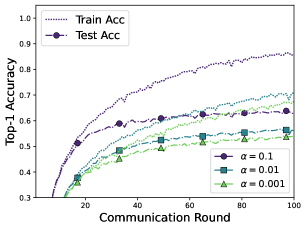
(a) FedAvg.

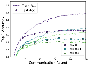
(b) SCAFFOLD.

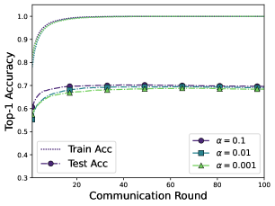
(c) TCT.

Figure 2: Training/test accuracy vs. communication round for FedAvg (left), SCAFFOLD (middle), and our algorithm TCT (right) on the CIFAR100 dataset with various degrees of non-iid-ness ($\mathrm{Dir}_{K}(\alpha)$ with $\alpha\in\{0.1,0.01,0.001\}$). Dotted lines represent the training accuracy, and dashdot lines with markers represent the test accuracy.

Table 2 displays the top-1 accuracy of all algorithm on the three tasks with varying degrees of data heterogeneity. We evaluated each algorithms on each task under four degrees of data heterogeneity. Smaller #C and $\alpha$ in Table 2 correspond to higher heterogeneity.

We find that the existing federated algorithms all suffer when data heterogeneity is high across all three tasks. For example, the top-1 accuracy of FedAvg on CIFAR-10 is $56.86\%$ when #C=2, which is much worse than the $90.43\%$ achieved in a more homogeneous setting (e.g. $\alpha=0.5$). In contrast, TCT achieves consistently strong performance, even in the face of high data heterogeneity. More specifically, TCT achieves the best top-1 accuracy performance across all settings except CIFAR-100 with $\alpha=0.5$, where TCT does only slightly worse than SCAFFOLD.

In absolute terms, we find that TCT is not affected much by data heterogeneity, with performance dropping by less than $1.5\%$ on CIFAR100 as $\alpha$ goes from $0.5$ to $0.001$. Moreover, our algorithm improves over existing methods by at least $15\%$ in the challenging cases, including FMNIST with #C=1, CIFAR-10 with #C=1 and #C=2, and CIFAR-100 with $\alpha=0.01$ and $\alpha=0.001$. And, perhaps surprisingly, our algorithm still performs relatively well in the extreme non-i.i.d. setting where each client sees only a single class.

Figure 2 compares the performances of FedAvg, SCAFFOLD, and TCT in more detail on CIFAR100 dataset with different degrees of data heterogeneity. We consider the Dirichlet distribution with parameter $\alpha\in\{0.1,0.01,0.001\}$ and compare the training and test accuracy of these three algorithms. As shown in Figures 2(a) and 2(b), both FedAvg and SCAFFOLD struggle when data heterogeneity is high: for both algorithms, test accuracy drops significantly when $\alpha$ decreases. In contrast, we see from Figure 2(c) that TCT maintains almost the same test accuracy for different $\alpha$. Furthermore, the same set of default parameters for our algorithm, including local learning rate and the number of local steps, is relatively robust to different levels of data heterogeneity.

5.3 Communication Efficiency

To understand the effectiveness of the local steps in our algorithm, we compare SCAFFOLD (used in TCT-Stage 2) to full batch gradient descent (GD) applied to the overparameterized linear regression problem in Stage 2 of TCT on these datasets. For our algorithm, we set local steps $M\in\{10^{2},10^{3}\}$ and use the default local learning rate. For full batch GD, we vary the learning rate from $10^{-5}$ to $10^{-1}$ and visualize the ones that do not diverge. The results are summarized in Figure 3. Each dotted line with square markers in Figure 3 corresponds to full batch GD with some learning rate. Across all three datasets, our proposed algorithm consistently outperforms full batch GD. Meanwhile, we find that more local steps for our algorithms lead to faster convergence across all settings. In particular, our algorithm converges within 20 communication rounds on CIFAR100 (as shown in Figure 3(c)). These results suggest that our proposed algorithm can largely leverage the local computation and improve communication efficiency.

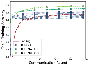
(a) FMNIST.

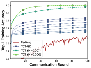
(b) CIFAR10.

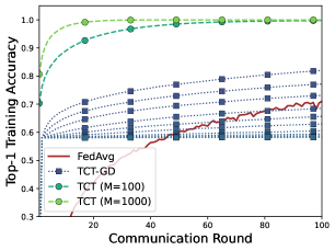
(c) CIFAR100.

Figure 3: Training accuracy vs. communication round for full batch gradient descent (GD) and TCT on FMNIST-[#C=2] (a), CIFAR10-[#C=2] (b), and CIFAR100-[$\alpha=0.01$] (c). Each dotted line with square markers represents the training accuracy of GD with some learning rate. Dashed lines with circle markers represent the training accuracy of TCT with different numbers of local steps. We also include the training accuracy results of FedAvg with learning rate $\eta=0.1$. We use TCT-GD to denote the variant of TCT which replaces SCAFFOLD with GD in Stage 2.

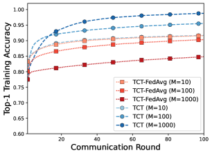
(a) FMNIST.

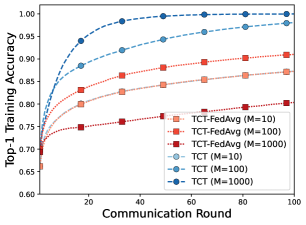
(b) CIFAR10.

(c) CIFAR100.

Figure 4: Comparing TCT to TCT-FedAvg for solving the overparameterized linear regression problem on (a) FMNIST-[#C=2], (b) CIFAR10-[#C=2], and (c) CIFAR100-[$\alpha=0.01$]. We use TCT-FedAvg to denote a variant of TCT that uses FedAvg instead of SCAFFOLD to perform linear regression in TCT-Stage 2. Dotted red lines with square markers represent the training accuracy of TCT-FedAvg with different numbers of local steps. Dashed blue red lines with circle markers represent the training accuracy of TCT with different numbers of local steps. A darker color means more local steps.

5.4 Ablations

Gradient correction. We investigate the role of gradient correction when solving overparameterized linear regression with eNTK features in TCT. We compare SCAFFOLD (used in TCT) to FedAvg on solving the regression problems and summarize the results in Figure 4. We use the default local learning rate and consider three different numbers of local steps for both algorithms, i.e., $M\in\{10,100,1000\}$. As shown in Figure 4, our approach largely outperforms FedAvg when the number of local steps is large ($M\geq 100$) across three datasets. We also find that the performance of FedAvg can even degrade when the number of local steps increases. For example, FedAvg with $M=1000$ performs the worst across all three datasets. In contrast to FedAvg, SCAFFOLD converges faster when the number of local steps increases. These observations highlight the importance of gradient correction in our algorithm.

Model weights for computing eNTK features.

To understand the impact of the model weights trained in Stage 1 of TCT, we evaluate TCT run with different $T_{1}$ parameters. We consider $T_{1}\in\{0,20,40,60,80,100\}$, where $T_{1}=0$ corresponds to randomly initialized weights. From Figure 5(a), we find that weights after FedAvg training are much more effective than weights at random initialization. Specifically, without FedAvg training, the eNTK (at random initialization) performs worse than standard FedAvg. In contrast, TCT significantly outperforms FedAvg by a large margin (roughly $20\%$ in test accuracy) when eNTK features are extracted from a FedAvg-trained model. Also, we find that TCT is stable with respect to the choice of communication rounds $T_{1}$ in Stage 1. For example, models trained by TCT with $T_{1}\geq 60$ achieve similar performance.

Effect of normalization.

In Figure 5(b), we investigate the role of normalization on TCT by comparing TCT run with normalized and unnormalized eNTK features. The same number of local steps ($M=500$) is applied for both settings. We tune the learning rate $\eta$ for each setting and plot the run that performs best (as measured in training accuracy). The results in Figure 5(b) suggest that the normalization step in TCT significantly improves the communication efficiency by increasing convergence speed. In particular, TCT with normalization converges to nearly $100\%$ training accuracy in approximately 40 communication rounds, which is much faster than TCT without normalization.

Pre-training vs. Bootstrapping.

In Appendix B.4, we explore the effect of starting from a pre-trained model instead of relying on bootstrapping to learn the features. We find that pre-training further improves the performance of TCT and completely erases the gap between centralized and federated learning.

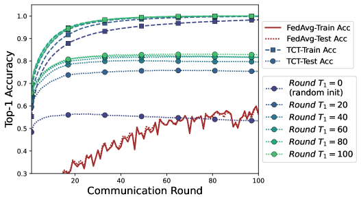
(a) Effect of FedAvg communication rounds in Stage 1.

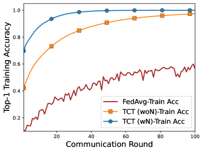
(b) Effect of normalization.

Figure 5: (a). We evaluate TCT on using checkpoints save at different communication rounds $T_{1}$ in Stage 1. $T_{1}=0$ corresponds to the randmon initialized model weights scenario (without FedAvg training). Dash lines with square markers represent the training accuracy, and dotted lines with circle makers represent the test accuracy. (b). We study the effect of pre-conditioning on TCT. TCT (wN) corresponds to the setting where eNTK features are normalized, and TCT (woN) corresponds to the without normalization step setting.

6 Conclusion

We have argued that nonconvexity poses a significant challenge for federated learning algorithms. We found that a neural network trained in such a manner does learn useful features, but fails to use them and thus has poor overall accuracy. To sidestep this issue, we proposed a train-convexify-train procedure: first, train the neural network using FedAvg; then, optimize (using SCAFFOLD) a convex approximation of the model obtained using its empirical neural tangent kernel. We showed that the first stage extracts meaningful features, whereas the second stage learns to utilize these features to obtain a highly performant model. The resulting algorithm is significantly faster and more stable to hyper-parameters than previous federated learning methods. Finally, we also showed that given a good pre-pretrained feature extractor, our convexify-train procedure fully closes the gap between centralized and federated learning.

Our algorithm adds to the growing body of work using eNTK to linearize neural networks and obtain tractable convex approximations. However, unlike most of these past works which only work with pre-trained models, our bootstrapping allows training models from scratch. Finally, we stress that the success of our approach underscores the need to revisit theoretical understanding of heterogeneous federated learning. Nonconvexity seems to play an outsized role but its effect in FL has hitherto been unexplored. In particular, black-box notions of difficulty such as gradient dissimilarity or distances between client optima seem insufficient to capture practical performance. It is likely that further progress in the field (e.g. federated pre-training of foundational models), will require tackling the issue of nonconvexity head on.

Appendix A Additional Details About Our Algorithm

A.1 An Efficient Implementation of SCAFFOLD

  Input: losses $\{L_{k}\}$, $k\in[K]$. Number of local steps $M$, server model $\theta^{0}$, learning rate $\eta$.

  Initialization:  client corrections $\{h_{k}^{-1}=\mathbf{0}\}$, local models$\{\widehat{\theta}^{0}_{i}\}=\theta^{0},\,\,k\in[K]$

  for round $t=0,1,\ldots,T$ do

     for clients $k=1,\ldots,K$ in parallel do

        Receive $\theta^{t}$ from server. Update correction

$$h_{k}^{t} =h_{k}^{t-1}+\tfrac{1}{M\eta}(\theta^{t}-\widehat{\theta}^{t}_{k}).$$ (2)

        Initialize client local model $\widehat{\theta}_{i}^{t,0}=\theta^{t}$.

        for $m=1,\dots,M$ do

           Update with a stochastic gradient sampled from local client data

$$\widehat{\theta}_{k}^{t,m+1} =\widehat{\theta}_{k}^{t,m}-\eta\left(\nabla L_{k}(\theta_{i}^{t,m};\xi_{k}^{t,m})-h_{k}^{t}\right).$$ (3)

        end for

        Set $\widehat{\theta}_{k}^{t+1}=\widehat{\theta}_{k}^{t,M+1}$. Communicate $\widehat{\theta}_{k}^{t+1}$ to server.

     end for

     Aggregate $\theta^{t+1}=\frac{1}{K}\sum_{k=1}^{K}\widehat{\theta}^{t+1}_{k}\,.$

  end for

Algorithm 1 Efficient implementation of SCAFFOLD

We describe a more communication efficient implementation of SCAFFOLD which is equivalent to Option II of SCAFFOLD from Karimireddy et al. [2020b]. Our implementation only requires a single model to be communicated between the client and server each round, making its communication complexity exactly equivalent to that of FedAvg. To see the equivalence, we prove that our implementation satisfies the following condition for any time step $t\geq 0$:

$$c_{k}^{t+1} :=\frac{1}{M}\sum_{m\in[M]}\nabla L_{k}(\theta_{k}^{t,m};\xi_{k}^{t,m})\,,\text{ and}$$

$$c^{t+1} :=\frac{1}{K}\sum_{k\in[K]}c_{k}^{t}\,,\text{ we maintain the invariant that}$$

$$h_{k}^{t+1} =c_{k}^{t+1}-c^{t+1}\,.$$

To see this, note that the local client model after updating in round $t$ is

$$\widehat{\theta}_{k}^{t+1} =\widehat{\theta}_{k}^{t,M+1}$$

$$=\theta^{t}-\eta\sum_{k\in[K]}\nabla L_{k}(\theta_{k}^{t,m};\xi_{k}^{t,m})-h_{k}^{t}$$

$$=\theta^{t}-M\eta(c_{k}^{t+1}-h_{k}^{t})\,.$$

By averaging this over the clients, we can see that the server model is

$$\theta^{t+1}=\theta^{t}-M\eta\Big{(}c^{t+1}-\frac{1}{K}\sum_{l\in[K]}h_{l}^{t}\Big{)}.$$

By induction, suppose that $h_{k}^{t}=c_{k}^{t}-c^{t}$. This implies that summing over the clients, it becomes zero; i.e., $\sum_{l\in[K]}h_{l}^{t}=0$. Plugging this and the previous computations, we have

$$h_{k}^{t+1} =h_{k}^{t}+\tfrac{1}{M\eta}(\theta^{t+1}-\widehat{\theta}^{t+1}_{k})$$

$$=h_{k}^{t}+\tfrac{1}{M\eta}(-M\eta c^{t+1}+M\eta(c_{k}^{t+1}-h_{k}^{t}))$$

$$=c_{k}^{t+1}-c^{t+1}\,.$$

For the base step at $t=0$, note that $h_{i}^{0}=\bm{0}$. This completes the proof by induction.

A.2 Additional Implementation Details

  Input: input dim $D$, output dim $C$, loss $\ell(\cdot,\cdot):\mathbb{R}^{C\times C}\rightarrow\mathbb{R}$, aggr. weights $\{w_{1},\dots,w_{K}\}$,

  model $f$ with parameters $\theta\in\mathbb{R}^{P}$: $f(x;\theta)=\phi\circ\omega~{}(x):\mathbb{R}^{D}\rightarrow\mathbb{R}^{C}$ (e.g., ResNet18), composed of a feature extractor $\phi:\mathbb{R}^{D}\rightarrow\mathbb{R}^{E}$ and final linear layer $\omega:\mathbb{R}^{E}\rightarrow\mathbb{R}^{C}$.

  Hyper-parameters: Local steps $M$ (default 500), Stage-1 lr $\eta_{1}$ (default 0.01), Stage-1 rounds $T_{1}$ (default 100), Stage-2 lr $\eta_{2}$ (default $5\cdot 10^{-5}$), Stage-2 rounds $T_{2}$ (default 100).

  Stage 1 (Bootstrapping):

  Initialize server model $\theta^{0}$.

  for round $t=0,1,\ldots,T_{1}$ do

     for clients $k=1,\ldots,K$ in parallel do

        Receive $\theta^{t}$ from server and initialize client local model $\widehat{\theta}_{k}^{t,0}=\theta^{t}$.

        for $m=1,\dots,M$ do

           Update with a mini-batch gradient sampled from local client data $(x_{k}^{t,m},y_{k}^{t,m})$

$$\widehat{\theta}_{k}^{t,m+1} =\widehat{\theta}_{k}^{t,m}-\eta_{i}\left(\nabla_{\theta}\ell(f(x_{k}^{t,m};\theta_{k}^{t,m}),y_{k}^{t,m})-h_{k}^{t}\right).$$

        end for

        Communicate $\widehat{\theta}_{k}^{t+1}$ to server.

     end for

     Aggregate $\theta^{t+1}=\frac{1}{\sum_{k}w_{k}}\sum_{k=1}^{K}w_{k}\widehat{\theta}^{t+1}_{k}\,.$

  end for

  Stage 2 (Convexification):

  Input: Bootstrapped parameters $\theta^{B}$ decomposed as $\theta^{B}=\phi^{B}\circ\omega^{B}$.

  Randomly re-initialize using fixed seed linear layer $\omega^{r}$ and define $\theta^{0}:=\phi^{B}\circ\omega^{r}$.

  [Comment:] Define basis vector $\mathbf{e_{1}}:=(1,0,\dots,0)$. For input $x$, $(\mathbf{e}_{1}^{\top}f(x;\theta^{0}))$ is the first logit.

  Optionally, compute a random sub-sampling mask $\mathscr{S}(\phi)$ over feature params using fixed seed .

  [Comment:] For a given input $x$, we will learn parameters $(\varphi,b)$ for prediction as

$$\hat{y}=\varphi^{\top}\phi_{\text{eNTK}}(x)+b,\quad\text{where}\quad\phi_{\text{eNTK}}(x):=\mathscr{S}\left(\nabla_{\phi}(\mathbf{e}_{1}^{\top}f(x;\phi^{B}\circ\omega^{r}))\right).$$

  Compute normalized eNTK features $\tilde{\phi}_{\text{eNTK}}(x)$ (mean 0 and variance 1) across clients.

  Also normalize targets to mean 0 using $\tilde{y}:=y-\frac{1}{C}\mathbf{1}$.

  Run SCAFFOLD (Algorithm 1) over params $\psi:=(\varphi,b)$ with learning rate $\eta_{2}$, local steps $M$, initial server params: $\psi^{0}=\mathbf{0}$, and client losses $\{L_{k}\}$ defined over the local data as

$$L_{k}(\psi):=\sum_{(x_{k},y_{k})}\left(\varphi^{\top}\tilde{\phi}_{\text{eNTK}}(x_{k})+b-\tilde{y}_{k}\right)^{2}\,.$$

Algorithm 2 TCT: complete pseudo-code

Algorithm 3 Compute eNTK Pseudocode, PyTorch-like

⬇

def compute_eNTK(model, X, num_params, subsample_size=100000, seed=123):

"""compute␣eNTK␣of␣input␣X␣with␣model"""

# model: model for linearization

# X: (n x d), n -- number of samples, d -- input dimension

# subsample_size: parameter of subsampling operation

# seed: random seed for subsampling operation

# num_params: total number of parameters for model

model.eval()

params = list(model.parameters())

torch.manual_seed(seed)

torch.cuda.manual_seed(seed)

random_index = torch.randperm(num_params)[:subsample_size]

eNTKs = torch.zeros((X.size()[0], subsample_size))

for i in range(X.size()[0]):

# compute eNTK for the i-th input

model.zero_grad()

model.forward(X[i:i+1])[0].backward()

eNTK = []

for param in params:

if param.requires_grad:

eNTK.append(param.grad.flatten())

eNTK = torch.cat(eNTK)

# subsampling

eNTKs[i, :] = eNTK[random_index]

return eNTKs

Additional details about linear regression in TCT.

In our experiments, we normalize the one-hot encoded label of each sample so that the normalized one-hot encoded label has mean 0. More specifically, we subtract $[1/C,\dots,1/C]^{\top}\in\mathbb{R}^{C\times 1}$ from the one-hot encoding label vector, where $C$ is the number of classes. Further,  Hui and Belkin [2020] show that performance for large number of classes can be improved by increasing the penalty for mis-classification and scaling the target from 1 to a larger value (e.g., 30). Achille et al. [2021] show that using Leaky-ReLU, and using K-FAC preconditioning further improves the performance. However, we do not explore such optimizations in this work–these (and other optimization tricks for least-squares regression) can be easily incorporated into our framework.

Local learning rate for TCT.

From our experiments, we find that small local learning rates ($\eta\leq 10^{-4}$) achieve good train/test accuracy performance for TCT with the normalization step. When the normalization step in TCT is applied, larger local learning rates diverge. Meanwhile, local learning rates from $[10^{-6},10^{-4}]$ achieve similar performance for TCT (as shown in Table 7). On the other hand, without the normalization step, TCT with large learning rate ($\eta\in[0.01,0.5]$) does not diverge. When running more communication rounds, TCT (without the normalization step) with large learning rate achieves similar performance as the default TCT (with the normalization step).

Additional details about Stage 2 of TCT.

To solve the linear regression problem in TCT-Stage 2, we use the full batch gradient in Eq. (3) of Algorithm 1 in our implementation.

Additional details about Figure 5.

We consider CIFAR10-[#C=2] in Figure 5(a) and 5(b).

Details about the total amount of compute.

We use NVIDIA 2080 Ti, A4000, and A100 GPUs, and our experiments required around 500 hours of GPU time.

Appendix B Additional Experimental Results

B.1 Additional Baselines

In comparison with FedAdam and FedDyn. We compare TCT to FedAdam [Reddi et al., 2021] and FedDyn [Acar et al., 2021] in Table 3. We consider four settings in Table 3, including CIFAR10 ($\texttt{\#C}=2$), CIFAR10 ($\alpha=0.1$), CIFAR100 ($\alpha=0.001$), and CIFAR100 ($\alpha=0.01$). For FedDyn, we perform similar hyperparameter selection as FedAvg; i.e., select local learning rate from $\{0.1,0.01,0.001\}$. For FedAdam, following recommendation by [Reddi et al., 2021], we set the global learning rate as $\eta_{\mathrm{global}}=0.1$ and select local learning rate from $\{10^{-1},10^{-1.5},10^{-2},10^{-2.5},10^{-3}\}$. Similar to results in Table 2, we find that TCT significantly outperforms the existing methods in high data heterogeneity settings.

Table 3: The top-1 test accuracy ($\%$) of our algorithm (TCT) vs. other federated learning algorithms (FedAdam [Reddi et al., 2021] and FedDyn [Acar et al., 2021]) evaluated on CIFAR10 and CIFAR100. We vary the degree of data heterogeneity by controlling the $\alpha$ parameter of the symmetric Dirichlet distribution $\mathrm{Dir}_{K}(\alpha)$ and the #C parameter for assigning how many labels each client owns. Higher accuracy is better. The highest top-1 accuracy in each setting is highlighted in bold.

Methods	Datasets
	CIFAR10 ($\texttt{\#C}=2$)	CIFAR10 ($\alpha=0.1$)		CIFAR100 ($\alpha=0.001$)	CIFAR100 ($\alpha=0.01$)
FedAdam [Reddi et al., 2021]	33.52%	62.57%		30.85%	37.16%
FedDyn [Acar et al., 2021]	51.67%	81.03%		50.86%	53.79%
TCT	83.02%	89.21%		69.07%	69.66%

B.2 Results of Other Architectures

In Section 5, we use batch normalization [Ioffe and Szegedy, 2015] as the default normalization layer on CIFAR10 and CIFAR100 datasets, and we denote the ResNet-18 with batch normalization layers by ResNet-18-BN. In Table 4, we consider group normalization [Wu and He, 2018] on CIFAR10 and CIFAR100 and let ResNet-18-GN denote the ResNet-18 with group normalization. We set num_groups=2 in group normalization layers. As shown in Table 4, TCT achieves better performance than FedAvg with ResNet-18-GN on both CIFAR10 and CIFAR100 datasets. Our experiments indicate that in extremely heterogeneous settings, group norm is insufficient to fix FedAvg.

Table 4: The top-1 test accuracy ($\%$) of our algorithm (TCT) vs. FedAvg(-GN) evaluated on CIFAR10 and CIFAR100. We vary the degree of data heterogeneity by controlling the $\alpha$ parameter of the symmetric Dirichlet distribution $\mathrm{Dir}_{K}(\alpha)$ and the #C parameter for assigning how many labels each client owns. Higher accuracy is better. The highest top-1 accuracy in each setting is highlighted in bold.

Datasets	Architectures	Methods	Non-i.i.d. degree
CIFAR-10			$\texttt{\#C}=1$	$\texttt{\#C}=2$	$\alpha=0.1$	$\alpha=0.5$
	ResNet-18-GN	FedAvg	21.23%	56.80%	84.72%	89.03%
	ResNet-18-BN	FedAvg	11.27%	56.86%	82.60%	90.43%
	ResNet-18-BN	TCT	49.92%	83.02%	89.21%	91.10%
CIFAR-100			$\alpha=0.001$	$\alpha=0.01$	$\alpha=0.1$	$\alpha=0.5$
	ResNet-18-GN	FedAvg	47.60%	48.60%	53.29%	55.39%
	ResNet-18-BN	FedAvg	53.89%	54.22%	63.49%	67.65%
	ResNet-18-BN	TCT	68.42%	69.07%	69.66%	69.68%

B.3 Additional Experimental Results of the Effect of Stage 1 Communication Round for TCT

In Figure 6, we provide additional results of the effect of $T_{1}$ for TCT on CIFAR10 and CIFAR100 datasets. We find that TCT outperforms existing algorithm across all $T_{1}$ communication rounds, where $T_{1}\geq 20$. Extending the number of rounds for the baseline algorithms to 200 rounds does not improve their performance. In contrast, running 60 rounds of bootstrapping using FedAvg followed by 40 rounds of TCT gives near-optimal performance across all settings.

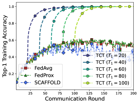
(a) CIFAR10-(#C=2), Train Accuracy.

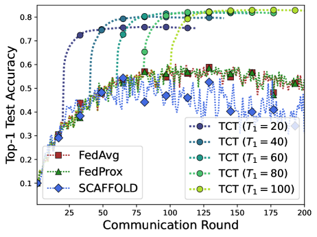
(b) CIFAR10-(#C=2), Test Accuracy.

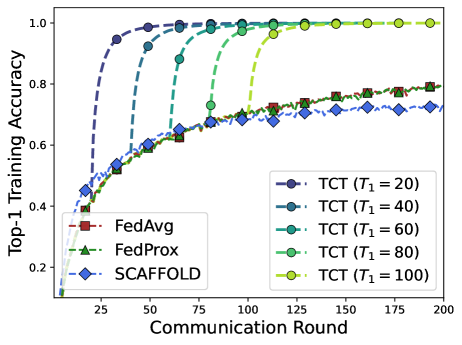
(c) CIFAR100-($\alpha=0.01$), Train Accuracy.

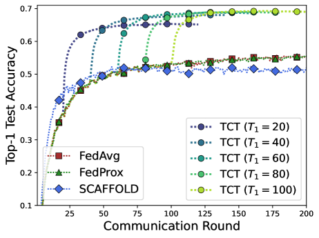
(d) CIFAR100-($\alpha=0.01$), Test Accuracy.

Figure 6: We evaluate TCT on using checkpoints saved at different communication rounds $T_{1}$ in Stage 1. We compare TCT to existing algorithm, including FedAvg, FedProx, and SCAFFOLD. For all three existing algorithms, we visualize the results of local learning rate $\eta=0.1$. The train/test accuracy results in the first $T_{1}$ communication rounds of TCT are the same as FedAvg. For example, “TCT ($T_{1}=20$)” corresponds to training the model with FedAvg for $T_{1}=20$ rounds in Stage 1 and then running $100$ rounds of SCAFFOLD for solving the linear regression problem in Stage 2. Plots (a) and (c) display training accuracy and (b) and (d) display test accuracy.

B.4 Additional Experimental Results of Pre-trained Models

In Table 5 and Figure 7, we provide additional results of the effect of pre-training for FedAvg and TCT on CIFAR10 and CIFAR100 datasets. For both methods, we use the ResNet-18 pre-trained on ImageNet-1k [He et al., 2016] as the initialization. We use FedAvg (last layer) to denote applying FedAvg on learning the last linear layer of the model, i.e., layers except for the last linear layer are freezed during training. Compared to results in Table 2, we find that using pre-trained model as initialization largely improves the performance of both FedAvg and TCT. However, FedAvg still suffers from data heterogeneity. In contrast, TCT achieves similar performance as the centralized setting on both datasets across different degrees of data heterogeneity.

Table 5: The top-1 test accuracy ($\%$) of our algorithm (TCT) vs. FedAvg evaluated on CIFAR10 and CIFAR100 with pre-trained model initialization. We vary the degree of data heterogeneity by controlling the $\alpha$ parameter of the symmetric Dirichlet distribution $\mathrm{Dir}_{K}(\alpha)$ and the #C parameter for assigning how many labels each client owns. Higher accuracy is better. The highest top-1 accuracy in each setting is highlighted in bold.

Methods	Datasets
	CIFAR10 ($\texttt{\#C}=2$)	CIFAR10 ($\alpha=0.1$)		CIFAR100 ($\alpha=0.001$)	CIFAR100 ($\alpha=0.01$)
Centralized	95.13%	95.13%		80.65%	80.65%
FedAvg (last layer)	63.60%	75.16%		50.40%	51.97%
FedAvg	64.73%	84.25%		62.23%	63.81%
TCT	92.97%	93.70%		79.25%	79.55%

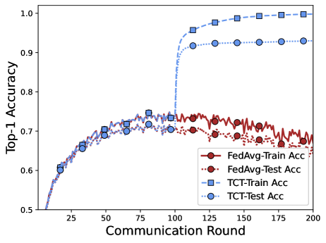
(a) CIFAR10-(#C=2).

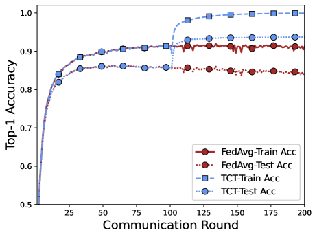
(b) CIFAR10-($\alpha=0.1$).

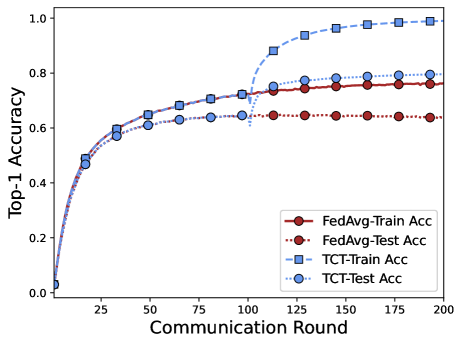
(c) CIFAR100-($\alpha=0.01$).

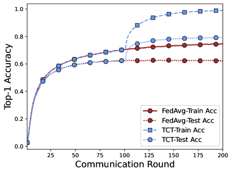
(d) CIFAR100-($\alpha=0.001$).

Figure 7: We evaluate FedAvg and TCT on CIFAR10 and CIFAR100 datasets with pre-trained ResNet-18. Plots (a) and (b) display training/test accuracy on the CIFAR10 dataset and (c) and (d) display training/test accuracy on the CIFAR100 dataset.

B.5 Additional Experimental Results of One-round Communication

In Table 6, we provide additional results of TCT on CIFAR10 and CIFAR100 datasets with one communication round in TCT-Stage 2. Specifically, we set the number of local steps $M=500$, local learning rate $\eta=0.00005$, and the total number of communication round $T=1$ in TCT-Stage 2. The results are summarized in Table 6. With only one communication round in TCT-Stage 2, TCT still achieves better performance than FedAvg in three out of four settings in Table 6. On the other hand, we recommend setting the communication round in TCT-Stage 2 larger than 10 for our method TCT in order to achieve satisfying performance.

Table 6: The top-1 test accuracy ($\%$) of our algorithm (TCT) on CIFAR10 and CIFAR100 with one communication round in TCT-Stage 2.

Methods	Datasets
	CIFAR10 ($\texttt{\#C}=2$)	CIFAR10 ($\alpha=0.01$)		CIFAR100 ($\alpha=0.001$)	CIFAR100 ($\alpha=0.01$)
FedAvg	56.86%	82.60%		53.89%	54.22%
TCT	83.02%	89.21%		68.42%	69.07%
TCT-OneRound	64.94%	82.62%		55.50%	57.51%

B.6 Additional Ablations

Effect of local learning rate for TCT and FedAdam.

As mentioned in Reddi et al. [2021], FedAdam is more robust to the choice of local learning rate compared to FedAvg. We conduct additional ablations on the effect of local learning rate for TCT as well as FedAdam [Reddi et al., 2021] on the CIFAR10 dataset. For each algorithm, we first select a base local learning rate $\eta_{\mathrm{base}}$ and then vary the local learning rate $\eta\in\{\eta_{\mathrm{base}}\cdot 10^{0},\eta_{\mathrm{base}}\cdot 10^{-0.5},\eta_{\mathrm{base}}\cdot 10^{-1.0},\eta_{\mathrm{base}}\cdot 10^{-1.5}\}$. The results are summarized in Table 7. Compared to FedAdam, we find that TCT is much less sensitive to the choice of local learning rate.

Table 7: The top-1 test accuracy ($\%$) of our algorithm (TCT) and FedAdam [Reddi et al., 2021] evaluated on the CIFAR10 dataset. We vary the local learning rate for both algorithms. Higher accuracy is better.

Datasets	Methods	Local learning rate
	($\eta_{\mathrm{base}}=10^{-4}$)	$\eta=\eta_{\mathrm{base}}\cdot 10^{0}$	$\eta=\eta_{\mathrm{base}}\cdot 10^{-0.5}$	$\eta=\eta_{\mathrm{base}}\cdot 10^{-1.0}$	$\eta=\eta_{\mathrm{base}}\cdot 10^{-1.5}$
CIFAR10-(#C=2)	TCT	82.12%	83.60%	83.51%	82.37%
CIFAR10-($\alpha=0.1$)	TCT	88.68%	89.27%	89.23%	89.15%
	($\eta_{\mathrm{base}}=10^{-1.5}$)	$\eta=\eta_{\mathrm{base}}\cdot 10^{0}$	$\eta=\eta_{\mathrm{base}}\cdot 10^{-0.5}$	$\eta=\eta_{\mathrm{base}}\cdot 10^{-1.0}$	$\eta=\eta_{\mathrm{base}}\cdot 10^{-1.5}$
CIFAR10-(#C=2)	FedAdam [Reddi et al., 2021]	31.29%	33.52%	26.20%	14.96%
CIFAR10-($\alpha=0.1$)	FedAdam [Reddi et al., 2021]	10.31%	37.26%	62.57%	49.18%

Effect of local learning rate and number of local steps for TCT.

We conduct additional ablations on the effect of both the local learning rate $\eta$ and the number of local steps $M$ for TCT on CIFAR10 and CIFAR100 datasets. The results in Table 8 and Table 9 indicate that TCT is robust to the choice of the local learning rate $\eta$ and the number of local steps $M$. We find that as the number of steps increases, the learning rate should predictably decrease. The performance is relatively stable along the diagonal, indicating that it is the product $M\cdot\eta$ which affects accuracy.

Table 8: The top-1 test accuracy ($\%$) of our algorithm (TCT) evaluated on the CIFAR10 dataset. We consider CIFAR10-(#C=2) and we set $\eta_{\mathrm{base}}=10^{-4}$. We vary both the local learning rate and the number of local steps for TCT. Higher accuracy is better.

Number of local steps	Local learning rate
	$\eta=\eta_{\mathrm{base}}\cdot 10^{0}$	$\eta=\eta_{\mathrm{base}}\cdot 10^{-0.5}$	$\eta=\eta_{\mathrm{base}}\cdot 10^{-1.0}$	$\eta=\eta_{\mathrm{base}}\cdot 10^{-1.5}$
$M=50$	83.51%	82.37%	80.67%	78.14%
$M=100$	83.59%	83.35%	81.73%	79.71%
$M=500$	82.12%	83.60%	83.51%	82.37%
$M=1000$	80.78%	82.92%	83.59%	83.35%

Table 9: The top-1 test accuracy ($\%$) of our algorithm (TCT) evaluated on the CIFAR100 dataset. We consider CIFAR100-($\alpha=0.01$) and we set $\eta_{\mathrm{base}}=10^{-4}$. We vary both the local learning rate and the number of local steps for TCT. Higher accuracy is better.

Number of local steps	Local learning rate
	$\eta=\eta_{\mathrm{base}}\cdot 10^{0}$	$\eta=\eta_{\mathrm{base}}\cdot 10^{-0.5}$	$\eta=\eta_{\mathrm{base}}\cdot 10^{-1.0}$	$\eta=\eta_{\mathrm{base}}\cdot 10^{-1.5}$
$M=50$	69.12%	67.31%	64.61%	61.34%
$M=100$	69.54%	68.48%	66.43%	63.42%
$M=500$	69.03%	69.60%	69.12%	67.31%
$M=1000$	68.38%	69.42%	69.54%	68.48%

References

- Acar et al. [2021] Durmus Alp Emre Acar, Yue Zhao, Ramon Matas, Matthew Mattina, Paul Whatmough, and Venkatesh Saligrama. Federated learning based on dynamic regularization. In International Conference on Learning Representations, 2021. URL https://openreview.net/forum?id=B7v4QMR6Z9w.
- Achille et al. [2021] Alessandro Achille, Aditya Golatkar, Avinash Ravichandran, Marzia Polito, and Stefano Soatto. Lqf: Linear quadratic fine-tuning. In Proceedings of the IEEE/CVF Conference on Computer Vision and Pattern Recognition, pages 15729–15739, 2021.
- Afonin and Karimireddy [2021] Andrei Afonin and Sai Praneeth Karimireddy. Towards model agnostic federated learning using knowledge distillation. arXiv preprint arXiv:2110.15210, 2021.
- Alistarh et al. [2017] Dan Alistarh, Demjan Grubic, Jerry Li, Ryota Tomioka, and Milan Vojnovic. QSGD: Communication-efficient SGD via gradient quantization and encoding. Advances in Neural Information Processing Systems, 30, 2017.
- [5] Haim Avron, Kenneth L. Clarkson, and David P. Woodruff. Sharper bounds for regularized data fitting. In Approximation, Randomization, and Combinatorial Optimization. Algorithms and Techniques, .
- Bagdasaryan et al. [2020] Eugene Bagdasaryan, Andreas Veit, Yiqing Hua, Deborah Estrin, and Vitaly Shmatikov. How to backdoor federated learning. In International Conference on Artificial Intelligence and Statistics, pages 2938–2948. PMLR, 2020.
- Blanchard et al. [2017] Peva Blanchard, El Mahdi El Mhamdi, Rachid Guerraoui, and Julien Stainer. Machine learning with adversaries: Byzantine tolerant gradient descent. Advances in Neural Information Processing Systems, 30, 2017.
- Bonawitz et al. [2021] Kallista Bonawitz, Peter Kairouz, Brendan McMahan, and Daniel Ramage. Federated learning and privacy: Building privacy-preserving systems for machine learning and data science on decentralized data. Queue, 19(5):87–114, 2021.
- Bonawitz et al. [2017] Keith Bonawitz, Vladimir Ivanov, Ben Kreuter, Antonio Marcedone, H Brendan McMahan, Sarvar Patel, Daniel Ramage, Aaron Segal, and Karn Seth. Practical secure aggregation for privacy-preserving machine learning. In Proceedings of the 2017 ACM SIGSAC Conference on Computer and Communications Security, pages 1175–1191, 2017.
- Bonawitz et al. [2019] Keith Bonawitz, Hubert Eichner, Wolfgang Grieskamp, Dzmitry Huba, Alex Ingerman, Vladimir Ivanov, Chloe Kiddon, Jakub Konečnỳ, Stefano Mazzocchi, Brendan McMahan, et al. Towards federated learning at scale: System design. Proceedings of Machine Learning and Systems, 1:374–388, 2019.
- Charles et al. [2021] Zachary Charles, Zachary Garrett, Zhouyuan Huo, Sergei Shmulyian, and Virginia Smith. On large-cohort training for federated learning. Advances in Neural Information Processing Systems, 34, 2021.
- Chayti and Karimireddy [2022] El Mahdi Chayti and Sai Praneeth Karimireddy. Optimization with access to auxiliary information. arXiv preprint arXiv:2206.00395, 2022.
- Collins et al. [2021] Liam Collins, Hamed Hassani, Aryan Mokhtari, and Sanjay Shakkottai. Exploiting shared representations for personalized federated learning. In International Conference on Machine Learning, pages 2089–2099. PMLR, 2021.
- Dean et al. [2012] Jeffrey Dean, Greg Corrado, Rajat Monga, Kai Chen, Matthieu Devin, Mark Mao, Marc’aurelio Ranzato, Andrew Senior, Paul Tucker, Ke Yang, et al. Large scale distributed deep networks. Advances in Neural Information Processing Systems, 25, 2012.
- Defazio et al. [2014] Aaron Defazio, Francis Bach, and Simon Lacoste-Julien. Saga: A fast incremental gradient method with support for non-strongly convex composite objectives. Advances in Neural Information Processing Systems, 27, 2014.
- Deng et al. [2020] Yuyang Deng, Mohammad Mahdi Kamani, and Mehrdad Mahdavi. Adaptive personalized federated learning. arXiv preprint arXiv:2003.13461, 2020.
- du Terrail et al. [2022] Jean Ogier du Terrail, Samy-Safwan Ayed, Edwige Cyffers, Felix Grimberg, Chaoyang He, Regis Loeb, Paul Mangold, Tanguy Marchand, Othmane Marfoq, Erum Mushtaq, et al. Flamby: Datasets and benchmarks for cross-silo federated learning in realistic settings. 2022.
- Fallah et al. [2020] Alireza Fallah, Aryan Mokhtari, and Asuman Ozdaglar. Personalized federated learning: A meta-learning approach. arXiv preprint arXiv:2002.07948, 2020.
- Fang et al. [2020] Minghong Fang, Xiaoyu Cao, Jinyuan Jia, and Neil Gong. Local model poisoning attacks to Byzantine-Robust federated learning. In 29th USENIX Security Symposium (USENIX Security 20), pages 1605–1622, 2020.
- Fort et al. [2020] Stanislav Fort, Gintare Karolina Dziugaite, Mansheej Paul, Sepideh Kharaghani, Daniel M Roy, and Surya Ganguli. Deep learning versus kernel learning: an empirical study of loss landscape geometry and the time evolution of the neural tangent kernel. In Advances in Neural Information Processing Systems, volume 33, pages 5850–5861, 2020.
- Fung et al. [2018] Clement Fung, Chris JM Yoon, and Ivan Beschastnikh. Mitigating sybils in federated learning poisoning. arXiv preprint arXiv:1808.04866, 2018.
- Goldblum et al. [2019] Micah Goldblum, Jonas Geiping, Avi Schwarzschild, Michael Moeller, and Tom Goldstein. Truth or backpropaganda? an empirical investigation of deep learning theory. arXiv preprint arXiv:1910.00359, 2019.
- Goyal et al. [2017] Priya Goyal, Piotr Dollár, Ross Girshick, Pieter Noordhuis, Lukasz Wesolowski, Aapo Kyrola, Andrew Tulloch, Yangqing Jia, and Kaiming He. Accurate, large minibatch SGD: Training Imagenet in 1 hour. arXiv preprint arXiv:1706.02677, 2017.
- Haddadpour et al. [2021] Farzin Haddadpour, Mohammad Mahdi Kamani, Aryan Mokhtari, and Mehrdad Mahdavi. Federated learning with compression: Unified analysis and sharp guarantees. In International Conference on Artificial Intelligence and Statistics, pages 2350–2358. PMLR, 2021.
- He et al. [2016] Kaiming He, Xiangyu Zhang, Shaoqing Ren, and Jian Sun. Deep residual learning for image recognition. In Proceedings of the IEEE conference on computer vision and pattern recognition, pages 770–778, 2016.
- He et al. [2022] Lie He, Sai Praneeth Karimireddy, and Martin Jaggi. Byzantine-robust decentralized learning via self-centered clipping. arXiv preprint arXiv:2202.01545, 2022.
- Hsieh et al. [2020] Kevin Hsieh, Amar Phanishayee, Onur Mutlu, and Phillip Gibbons. The non-iid data quagmire of decentralized machine learning. In International Conference on Machine Learning, pages 4387–4398. PMLR, 2020.
- Hsu et al. [2019] Tzu-Ming Harry Hsu, Hang Qi, and Matthew Brown. Measuring the effects of non-identical data distribution for federated visual classification. arXiv preprint arXiv:1909.06335, 2019.
- Hui and Belkin [2020] Like Hui and Mikhail Belkin. Evaluation of neural architectures trained with square loss vs cross-entropy in classification tasks. arXiv preprint arXiv:2006.07322, 2020.
- Iandola et al. [2016] Forrest N Iandola, Matthew W Moskewicz, Khalid Ashraf, and Kurt Keutzer. Firecaffe: near-linear acceleration of deep neural network training on compute clusters. In Proceedings of the IEEE Conference on Computer Vision and Pattern Recognition, pages 2592–2600, 2016.
- Ioffe and Szegedy [2015] Sergey Ioffe and Christian Szegedy. Batch normalization: Accelerating deep network training by reducing internal covariate shift. In International conference on machine learning, pages 448–456. PMLR, 2015.
- Izmailov et al. [2018] Pavel Izmailov, Dmitrii Podoprikhin, Timur Garipov, Dmitry Vetrov, and Andrew Gordon Wilson. Averaging weights leads to wider optima and better generalization. arXiv preprint arXiv:1803.05407, 2018.
- Jacot et al. [2018] Arthur Jacot, Franck Gabriel, and Clément Hongler. Neural tangent kernel: Convergence and generalization in neural networks. Advances in Neural Information Processing Systems, 31, 2018.
- Johnson and Zhang [2013] Rie Johnson and Tong Zhang. Accelerating stochastic gradient descent using predictive variance reduction. Advances in Neural Information Processing Systems, 26, 2013.
- Jones and Tonetti [2020] Charles I Jones and Christopher Tonetti. Nonrivalry and the economics of data. American Economic Review, 110(9):2819–58, 2020.
- Kairouz et al. [2021] Peter Kairouz, H. Brendan McMahan, et al. Advances and open problems in federated learning. Foundations and Trends® in Machine Learning, 14(1–2):1–210, 2021.
- Karimireddy et al. [2020a] Sai Praneeth Karimireddy, Martin Jaggi, Satyen Kale, Mehryar Mohri, Sashank J Reddi, Sebastian U Stich, and Ananda Theertha Suresh. Mime: Mimicking centralized stochastic algorithms in federated learning. arXiv preprint arXiv:2008.03606, 2020a.
- Karimireddy et al. [2020b] Sai Praneeth Karimireddy, Satyen Kale, Mehryar Mohri, Sashank Reddi, Sebastian Stich, and Ananda Theertha Suresh. Scaffold: Stochastic controlled averaging for federated learning. In International Conference on Machine Learning, pages 5132–5143. PMLR, 2020b.
- Karimireddy et al. [2021] Sai Praneeth Karimireddy, Lie He, and Martin Jaggi. Byzantine-robust learning on heterogeneous datasets via bucketing. In International Conference on Learning Representations, 2021.
- Krizhevsky et al. [2009] Alex Krizhevsky, Geoffrey Hinton, et al. Learning multiple layers of features from tiny images. 2009.
- Kulkarni et al. [2020] Viraj Kulkarni, Milind Kulkarni, and Aniruddha Pant. Survey of personalization techniques for federated learning. In 2020 Fourth World Conference on Smart Trends in Systems, Security and Sustainability (WorldS4), pages 794–797. IEEE, 2020.
- Kulynych et al. [2020] Bogdan Kulynych, David Madras, Smitha Milli, Inioluwa Deborah Raji, Angela Zhou, and Richard Zemel. Participatory approaches to machine learning. International Conference on Machine Learning Workshop, 2020.
- Lee et al. [2019] Jaehoon Lee, Lechao Xiao, Samuel Schoenholz, Yasaman Bahri, Roman Novak, Jascha Sohl-Dickstein, and Jeffrey Pennington. Wide neural networks of any depth evolve as linear models under gradient descent. Advances in Neural Information Processing Systems, 32, 2019.
- Li et al. [2021a] Qinbin Li, Yiqun Diao, Quan Chen, and Bingsheng He. Federated learning on non-iid data silos: An experimental study. arXiv preprint arXiv:2102.02079, 2021a.
- Li et al. [2021b] Qinbin Li, Bingsheng He, and Dawn Song. Model-contrastive federated learning. In Proceedings of the IEEE/CVF Conference on Computer Vision and Pattern Recognition, pages 10713–10722, 2021b.
- Li et al. [2019] Tian Li, Maziar Sanjabi, Ahmad Beirami, and Virginia Smith. Fair resource allocation in federated learning. arXiv preprint arXiv:1905.10497, 2019.
- Li et al. [2020] Tian Li, Anit Kumar Sahu, Manzil Zaheer, Maziar Sanjabi, Ameet Talwalkar, and Virginia Smith. Federated optimization in heterogeneous networks. Proceedings of Machine Learning and Systems, 2:429–450, 2020.
- Lin et al. [2020] Tao Lin, Lingjing Kong, Sebastian U Stich, and Martin Jaggi. Ensemble distillation for robust model fusion in federated learning. Advances in Neural Information Processing Systems, 33:2351–2363, 2020.
- Lin et al. [2021] Tao Lin, Sai Praneeth Karimireddy, Sebastian U Stich, and Martin Jaggi. Quasi-global momentum: Accelerating decentralized deep learning on heterogeneous data. arXiv preprint arXiv:2102.04761, 2021.
- Long [2021] Philip M Long. Properties of the after kernel. arXiv preprint arXiv:2105.10585, 2021.
- Lyu et al. [2020] Lingjuan Lyu, Han Yu, and Qiang Yang. Threats to federated learning: A survey. arXiv preprint arXiv:2003.02133, 2020.
- McMahan et al. [2017] Brendan McMahan, Eider Moore, Daniel Ramage, Seth Hampson, and Blaise Aguera y Arcas. Communication-efficient learning of deep networks from decentralized data. In Artificial Intelligence and Statistics, pages 1273–1282. PMLR, 2017.
- Mishchenko et al. [2022] Konstantin Mishchenko, Grigory Malinovsky, Sebastian Stich, and Peter Richtárik. Proxskip: Yes! local gradient steps provably lead to communication acceleration! finally! arXiv preprint arXiv:2202.09357, 2022.
- Mohri et al. [2019] Mehryar Mohri, Gary Sivek, and Ananda Theertha Suresh. Agnostic federated learning. In International Conference on Machine Learning, pages 4615–4625. PMLR, 2019.
- Mothukuri et al. [2021] Viraaji Mothukuri, Reza M Parizi, Seyedamin Pouriyeh, Yan Huang, Ali Dehghantanha, and Gautam Srivastava. A survey on security and privacy of federated learning. Future Generation Computer Systems, 115:619–640, 2021.
- Mu et al. [2020] Fangzhou Mu, Yingyu Liang, and Yin Li. Gradients as features for deep representation learning. arXiv preprint arXiv:2004.05529, 2020.
- Ozkara et al. [2021] Kaan Ozkara, Navjot Singh, Deepesh Data, and Suhas Diggavi. Quped: Quantized personalization via distillation with applications to federated learning. Advances in Neural Information Processing Systems, 34, 2021.
- Pentland et al. [2021] Alex Pentland, Alexander Lipton, and Thomas Hardjono. Building the New Economy: Data as Capital. MIT Press, 2021.
- Ramaswamy et al. [2020] Swaroop Ramaswamy, Om Thakkar, Rajiv Mathews, Galen Andrew, H Brendan McMahan, and Françoise Beaufays. Training production language models without memorizing user data. arXiv preprint arXiv:2009.10031, 2020.
- Reddi et al. [2021] Sashank J. Reddi, Zachary Charles, Manzil Zaheer, Zachary Garrett, Keith Rush, Jakub Konečný, Sanjiv Kumar, and Hugh Brendan McMahan. Adaptive federated optimization. In International Conference on Learning Representations, 2021. URL https://openreview.net/forum?id=LkFG3lB13U5.
- Shi et al. [2021] Yuxin Shi, Han Yu, and Cyril Leung. A survey of fairness-aware federated learning. arXiv preprint arXiv:2111.01872, 2021.
- Singh and Jaggi [2020] Sidak Pal Singh and Martin Jaggi. Model fusion via optimal transport. Advances in Neural Information Processing Systems, 33:22045–22055, 2020.
- So et al. [2020] Jinhyun So, Başak Güler, and A Salman Avestimehr. Byzantine-resilient secure federated learning. IEEE Journal on Selected Areas in Communications, 39(7):2168–2181, 2020.
- Stich and Karimireddy [2020] Sebastian U Stich and Sai Praneeth Karimireddy. The error-feedback framework: Better rates for sgd with delayed gradients and compressed updates. Journal of Machine Learning Research, 21:1–36, 2020.
- Sun et al. [2019] Ziteng Sun, Peter Kairouz, Ananda Theertha Suresh, and H Brendan McMahan. Can you really backdoor federated learning? arXiv preprint arXiv:1911.07963, 2019.
- Suresh et al. [2017] Ananda Theertha Suresh, X Yu Felix, Sanjiv Kumar, and H Brendan McMahan. Distributed mean estimation with limited communication. In International Conference on Machine Learning, pages 3329–3337. PMLR, 2017.
- Tan et al. [2021] Yue Tan, Guodong Long, Lu Liu, Tianyi Zhou, Qinghua Lu, Jing Jiang, and Chengqi Zhang. Fedproto: Federated prototype learning over heterogeneous devices. arXiv preprint arXiv:2105.00243, 2021.
- Wang et al. [2020a] Hongyi Wang, Kartik Sreenivasan, Shashank Rajput, Harit Vishwakarma, Saurabh Agarwal, Jy-yong Sohn, Kangwook Lee, and Dimitris Papailiopoulos. Attack of the tails: Yes, you really can backdoor federated learning. Advances in Neural Information Processing Systems, 33:16070–16084, 2020a.
- Wang et al. [2019a] Jianyu Wang, Vinayak Tantia, Nicolas Ballas, and Michael Rabbat. Slowmo: Improving communication-efficient distributed sgd with slow momentum. arXiv preprint arXiv:1910.00643, 2019a.
- Wang et al. [2020b] Jianyu Wang, Qinghua Liu, Hao Liang, Gauri Joshi, and H Vincent Poor. Tackling the objective inconsistency problem in heterogeneous federated optimization. Advances in Neural Information Processing Systems, 33:7611–7623, 2020b.
- Wang et al. [2021] Jianyu Wang, Zachary Charles, Zheng Xu, Gauri Joshi, H Brendan McMahan, Maruan Al-Shedivat, Galen Andrew, Salman Avestimehr, Katharine Daly, Deepesh Data, et al. A field guide to federated optimization. arXiv preprint arXiv:2107.06917, 2021.
- Wang et al. [2022] Jianyu Wang, Rudrajit Das, Gauri Joshi, Satyen Kale, Zheng Xu, and Tong Zhang. On the unreasonable effectiveness of federated averaging with heterogeneous data. arXiv preprint arXiv:2206.04723, 2022.
- Wang et al. [2019b] Shiqiang Wang, Tiffany Tuor, Theodoros Salonidis, Kin K Leung, Christian Makaya, Ting He, and Kevin Chan. Adaptive federated learning in resource constrained edge computing systems. IEEE Journal on Selected Areas in Communications, 37(6):1205–1221, 2019b.
- Wei et al. [2022] Alexander Wei, Wei Hu, and Jacob Steinhardt. More than a toy: Random matrix models predict how real-world neural representations generalize. arXiv preprint arXiv:2203.06176, 2022.
- Woodworth et al. [2020] Blake E Woodworth, Kumar Kshitij Patel, and Nati Srebro. Minibatch vs local sgd for heterogeneous distributed learning. Advances in Neural Information Processing Systems, 33:6281–6292, 2020.
- Wortsman et al. [2022] Mitchell Wortsman, Gabriel Ilharco, Samir Yitzhak Gadre, Rebecca Roelofs, Raphael Gontijo-Lopes, Ari S Morcos, Hongseok Namkoong, Ali Farhadi, Yair Carmon, Simon Kornblith, et al. Model soups: averaging weights of multiple fine-tuned models improves accuracy without increasing inference time. arXiv preprint arXiv:2203.05482, 2022.
- Wu et al. [2020] Qiong Wu, Kaiwen He, and Xu Chen. Personalized federated learning for intelligent IoT applications: A cloud-edge based framework. IEEE Open Journal of the Computer Society, 1:35–44, 2020.
- Wu and He [2018] Yuxin Wu and Kaiming He. Group normalization. In Proceedings of the European Conference on Computer Vision (ECCV), pages 3–19, 2018.
- Xiao et al. [2017] Han Xiao, Kashif Rasul, and Roland Vollgraf. Fashion-MNIST: a novel image dataset for benchmarking machine learning algorithms. arXiv preprint arXiv:1708.07747, 2017.
- Yu et al. [2021] Fuxun Yu, Weishan Zhang, Zhuwei Qin, Zirui Xu, Di Wang, Chenchen Liu, Zhi Tian, and Xiang Chen. Fed2: Feature-aligned federated learning. In Proceedings of the 27th ACM SIGKDD Conference on Knowledge Discovery & Data Mining, pages 2066–2074, 2021.
- Zancato et al. [2020] Luca Zancato, Alessandro Achille, Avinash Ravichandran, Rahul Bhotika, and Stefano Soatto. Predicting training time without training. Advances in Neural Information Processing Systems, 33:6136–6146, 2020.