Stability analysis of non-Abelian electric fields

Abstract

We study the stability of fluctuations around a homogeneous non-Abelian electric field background that is of a form that is protected from Schwinger pair production. Our analysis identifies the unstable modes and we find a limiting set of parameters for which there are no instabilities. We discuss potential implications of our analysis for confining strings in non-Abelian gauge theories.

I Introduction

In pure non-Abelian gauge theory, the gauge fields carry non-Abelian electric charge. Hence a non-Abelian electric field is susceptible to decay via the Schwinger pair production of gauge field quanta Matinyan and Savvidy (1978); Brown and Weisberger (1979); Yildiz and Cox (1980); Ambjorn and Hughes (1982a, b); Cooper and Nayak (2006); Nayak and van Nieuwenhuizen (2005); Cooper et al. (2008); Nair and Yelnikov (2010); Ragsdale and Singleton (2017); Cardona and Vachaspati (2021). However, confining electric field tube configurations do not decay, leading to a quandary – how are electric flux tubes stable to Schwinger pair production? This question was raised and investigated in Vachaspati (2022). The essential idea is that there are many gauge inequivalent ways of constructing an electric field in non-Abelian theory Brown and Weisberger (1979). The straight-forward embedding of the Maxwell gauge field in the non-Abelian theory is indeed unstable to Schwinger pair production. However, other inequivalent gauge fields, that nonetheless produce the same electric field, are protected against quantum dissipation. Such gauge field configurations are candidates for describing confining electric flux tubes.

In a quantum theory, there will be fluctuations about the electric field background and these fluctuations will ultimately be quantized. It is therefore of interest to determine the fluctuation eigenfrequencies and eigenmodes, and especially to determine if there are any unstable fluctuations. The question has been addressed in Refs. Bazak and Mrowczynski (2022a, b) for a homogeneous electric field where a number of unstable modes were found. However those analyses did not eliminate fluctuations that were inconsistent with their adopted gauge conditions; neither did they account for extra conditions imposed by the reality of the gauge fields. Indeed we shall see that these conditions are critical for the stability analysis. The earlier analyses were also limited to either a special point in the parameter space of the background electric field Bazak and Mrowczynski (2022a) or to only the zero momentum modes Bazak and Mrowczynski (2022b).

We start by describing the homogeneous electric field in SU(2) non-Abelian gauge theory in Sec. II. Then we consider small fluctuations around the background electric field in Sec. III, expand the fluctuations in modes in Sec. IV. The modes get classified according to whether they are longitudinal or transverse, and whether they are orthogonal to the electric field. The transverse-orthogonal (TO) modes are discussed in Sec. V while the transverse-nonorthogonal (TN) and longitudinal (L) modes are discussed together in Sec. VI as they are coupled. Unstable TO modes are found to exist in the infrared and depend on the parameters entering the background configuration, and an interesting limit is found for which the unstable TO modes are absent. The analysis for the TN and L modes is significantly more complicated and we limit ourselves to some special cases, for example large or small wavenumbers, and for wave vectors parallel and orthogonal to the electric field. Our results again show some unstable modes in the infrared and once more, just as in the case of TO modes, we find that there are no unstable modes in the special limit of background parameters.

Our results are summarized in Sec. VII where we also discuss other ideas. The reader not interested in the technicalities of the analysis can find details about the electric field background in Sec. II and then proceed to the conclusions in Sec. VII.

II Electric field background

Consider the $SU(2)$ pure gauge theory,

$$L=-\frac{1}{4g^{2}}W_{\mu\nu}^{a}W^{\mu\nu a}+j_{\mu}^{a}W^{\mu a}$$ (1)

where $g$ is the gauge coupling, $\mu,\nu=0,1,2,3$ are Lorentz indices and $a=1,2,3$ is the color index. The current $j_{\mu}^{a}$ is an external current which will be specified below. The field strength $W_{\mu\nu}^{a}$ is given in terms of the gauge potential $W_{\mu}^{a}$ by,

$$W_{\mu\nu}^{a}\equiv\partial_{\mu}W_{\nu}^{a}-\partial_{\mu}W_{\nu}^{a}+\epsilon^{abc}W_{\mu}^{b}W_{\nu}^{c}.$$ (2)

The gauge field equations of motion are

$${\cal D}_{\nu}W^{\mu\nu a}=j^{\mu a}$$ (3)

where

$${\cal D}_{\nu}W^{\mu\nu a}\equiv\partial_{\nu}W^{\mu\nu a}+\epsilon^{abc}W_{\nu}^{b}W^{\mu\nu c}.$$ (4)

We wish to consider the stability of a class of gauge fields that give rise to homogeneous electric fields that we treat as a background. The gauge fields are

$$A_{\mu}^{\pm}\equiv A_{\mu}^{1}\pm iA_{\mu}^{2}=-\epsilon e^{\pm i\Omega t}\partial_{\mu}z,\ \ A_{\mu}^{3}=0$$ (5)

where $\epsilon$ and $\Omega$ are parameters that label members of the class, and $z$ is the spatial $z$ coordinate. The electric field is gauge equivalent to Vachaspati (2022),

$$E^{a}_{i}=\epsilon\Omega\delta^{a3}\delta_{iz}$$ (6)

and the amplitude of the electric field is

$$E=\epsilon\Omega$$ (7)

As shown in Ref. Brown and Weisberger (1979), gauge fields with distinct values of $\Omega^{2}$, even for the same value of $E$, are gauge inequivalent.

In the two dimensional parameter space $(\epsilon,\Omega)$, the electric field is constant whenever $\epsilon\Omega$ is constant. We will find that the limit $\epsilon\to 0$, $\Omega\to\infty$ but with $E=\epsilon\Omega$ held constant to be of interest from the point of view of stability.

The external currents $j_{\mu}^{a}$ in (1) are chosen such that the background is a solution of the classical equations of motion. Therefore

$$j^{\mu a}={\cal D}^{(A)}_{\nu}A^{\mu\nu a}$$ (8)

which gives

$$j_{\mu}^{\pm}\equiv j_{\mu}^{1}\pm ij_{\mu}^{2}=-\frac{\epsilon\Omega^{2}}{2}e^{\pm i\Omega t}\partial_{\mu}z,\ \ j_{\mu}^{3}=0.$$ (9)

For the purposes of the stability analysis we simply assume that this is an external current, though it is possible that the currents can arise semiclassically as discussed in Ref. Vachaspati (2022) and summarized in Sec. VII.

III Fluctuations

We now consider small perturbations around the background,

$$W_{\mu}^{a}=A_{\mu}^{a}+q_{\mu}^{a}.$$ (10)

Inserting this into the equations of motion, (3), and working to linear order in the perturbations $q_{\mu}^{a}$ we get,

$$\partial_{\nu}q^{\mu\nu a}+\epsilon^{abc}(A_{\nu}^{b}q^{\mu\nu c}+q_{\nu}^{b}A^{\mu\nu c})=0$$ (11)

where

$$q_{\mu\nu}^{a}=\partial_{\mu}q_{\nu}^{a}-\partial_{\nu}q_{\mu}^{a}+\epsilon^{abc}(A_{\mu}^{b}q_{\nu}^{c}-A_{\nu}^{b}q_{\mu}^{c})$$ (12)

and

$$A_{\mu\nu}^{a}=\partial_{\mu}A_{\nu}^{a}-\partial_{\nu}A_{\mu}^{a}+\epsilon^{abc}A_{\mu}^{b}A_{\nu}^{c}$$ (13)

which, with our chosen background,

$$A^{\pm}_{\mu}=-\epsilon e^{\pm i\Omega t}\,\partial_{\mu}z,\ \ A^{3}_{\mu}=0,$$ (14)

gives

$$A_{\mu\nu}^{\pm}=\pm iEe^{\pm i\Omega t}(\partial_{\mu}z\partial_{\nu}t-\partial_{\nu}z\partial_{\mu}t),\ \ A_{\mu\nu}^{3}=0$$ (15)

We will be adopting temporal gauge ($W_{0}^{a}=0$), so $q_{0}^{a}=0$.

IV Mode Expansion

We first define fluctuations in a “rotating frame”, $Q^{a}_{i}$, as follows,

$$q^{1}_{i}+iq^{2}_{i}\equiv e^{i\Omega t}(Q^{1}_{i}+iQ^{2}_{i}),\ \ q^{3}_{i}\equiv Q^{3}_{i}$$ (16)

where $Q^{a}_{i}$ are real. Next we expand $Q_{i}^{a}$ in spatial and temporal Fourier modes as follows,

$$Q_{i}^{a} = \int\frac{d^{3}k}{(2\pi)^{3}}e^{-i\omega_{\bf k}t}e^{i{\bf k}\cdot{\bf x}}p_{i,{\bf k}}^{a}$$ (17)

where $p_{i,{\bf k}}^{a}$ are the Fourier amplitudes.

While $\omega_{\bf k}$ can in general be complex, the reality of the fields $Q_{i}^{a}$ constrain physical values of $\omega_{\bf k}$ and $p_{i}^{a}$ to satisfy,

$$\omega_{\bf k}^{*}=-\omega_{-{\bf k}},\ \ (p^{a}_{i,{\bf k}})^{*}=p^{a}_{i,-{\bf k}}.$$ (18)

In what follows we will consider a single ${\bf k}$ mode and drop the ${\bf k}$ subscripts, e.g. we write $\omega_{\bf k}$ simply as $\omega$.

Inserting the Fourier expansion into (11) gives 3 constraint equations (the Gauss constraints) and 9 equations of motion for the 9 components of $p_{i}^{a}$. The constraints are,

$$\omega{\bf k}\cdot{\bf p}^{1}-i\Omega{\bf k}\cdot{\bf p}^{2}+\epsilon\Omega p_{z}^{3} = 0$$ (19)

$$\omega{\bf k}\cdot{\bf p}^{2}+i\Omega{\bf k}\cdot{\bf p}^{1}-i\epsilon\omega p_{z}^{3} = 0$$ (20)

$$\omega{\bf k}\cdot{\bf p}^{3}+i\epsilon\omega p_{z}^{2}-2\epsilon\Omega p_{z}^{1} = 0$$ (21)

and the equations of motion are,

$$\hskip-42.67912pt(-\omega^{2}+k^{2}-\Omega^{2}){\bf p}^{1}+i2\omega\Omega{\bf p}^{2}-({\bf k}\cdot{\bf p}^{1}){\bf k}=0$$ (22)

$$\hskip-42.67912pt(-\omega^{2}+k^{2}-\Omega^{2}+\epsilon^{2}){\bf p}^{2}-i2\omega\Omega{\bf p}^{1}-({\bf k}\cdot{\bf p}^{2}){\bf k}$$

$$\hskip-14.22636pt-\epsilon(-i{\bf k}\cdot{\bf p}^{3}+\epsilon p_{z}^{2}){\hat{z}}+i\epsilon p_{z}^{3}{\bf k}-i2\epsilon k_{z}{\bf p}^{3}=0$$ (23)

$$\hskip-28.45274pt(-\omega^{2}+k^{2}+\epsilon^{2}){\bf p}^{3}-({\bf k}\cdot{\bf p}^{3}){\bf k}-i\epsilon({\bf k}\cdot{\bf p}^{2}){\hat{z}}$$

$$\hskip 42.67912pt+i2\epsilon k_{z}{\bf p}^{2}-i\epsilon p_{z}^{2}{\bf k}-\epsilon^{2}p_{z}^{3}{\hat{z}}=0$$ (24)

where we have now employed the vector notation: ${\bf p}^{a}=(p^{a}_{1},p^{a}_{2},p^{a}_{3})$ and ${\bf k}\cdot{\bf p}^{a}=k_{i}p^{a}_{i}$. It is straightforward to check that any solution of Eqs. (19)-(24) with $\omega_{\bf k}^{*}=-\omega_{-{\bf k}}$ will also satisfy $(p^{a}_{i,{\bf k}})^{*}=p^{a}_{i,-{\bf k}}$, i.e. Eqs. (19)-(24) are consistent with the reality conditions in (18).

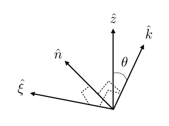
Figure 1: The triad of orthonormal vectors $\{{\hat{k}},{\hat{n}},{\hat{\xi}}\}$ and the direction of the electric field along ${\hat{z}}$. The vectors ${\hat{k}}$, ${\hat{\xi}}$ and ${\hat{z}}$ are in a plane while ${\hat{n}}$ is normal to the plane.

The variables ${\bf p}^{a}$ have a natural decomposition in a basis of spatial vectors $\{{\hat{k}},{\hat{n}},{\hat{\xi}}\}$ (see Fig. 1) where

$$\hat{k}=\frac{{\bf k}}{k},\ \ \hat{n}=\hat{\xi}\times\hat{k},\ \ \hat{\xi}=\frac{\hat{z}-c\hat{k}}{s}$$ (25)

For convenience, we have denoted $c\equiv\hat{k}\cdot\hat{z}=\cos\theta$ and $s=|\hat{z}\times\hat{k}|=\sin\theta$ where $\theta$ is the angle between $\hat{k}$ and $\hat{z}$. Then we have the useful relation

$$\hat{z}=s\hat{\xi}+c\hat{k}.$$ (26)

Next write

$${\bf p}^{a}=\alpha_{a}\hat{k}+\beta_{a}\hat{n}+\gamma_{a}\hat{\xi}$$ (27)

The $\{\alpha_{a}\}$ modes, with polarization in the $\hat{k}$ direction, are longitudinal. The $\{\beta_{a}\}$ modes are polarized in the $\hat{n}$ direction and are transverse and also polarized orthogonal to the electric field. The $\{\gamma_{a}\}$ modes are transverse and polarized in the $\hat{\xi}$ direction which is at an angle $\pi/2-\theta$ to the electric field. We shall call $\{\alpha_{a}\}$ the “longitudinal” (L) modes, the $\{\beta_{a}\}$ as the “transverse-orthogonal” (TO) modes, and the $\{\gamma_{a}\}$ as the “transverse-nonorthogonal” (TN) modes. Note that for $\theta=0$, the TN modes are also orthogonal to the electric field and coincide with TO modes.

The constraints and equations of motion in (19)-(21) and (22)-(24) can be written in terms of the 9 functions $\{\alpha_{a},\beta_{a},\gamma_{a}\}$. The constraints are,

$$\omega k\alpha_{1}-i\Omega k\alpha_{2}+\epsilon\Omega c\alpha_{3}+\epsilon\Omega s\gamma_{3}=0$$ (28)

$$\omega k\alpha_{2}+i\Omega k\alpha_{1}-i\epsilon\omega c\alpha_{3}-i\epsilon\omega s\gamma_{3}=0$$ (29)

$$\hskip-28.45274pt\omega k\alpha_{3}+i\epsilon\omega c\alpha_{2}+i\epsilon\omega s\gamma_{2}-2\epsilon\Omega c\alpha_{1}-2\epsilon\Omega s\gamma_{1}=0$$ (30)

Note that the constraints do not involve the $\{\beta_{a}\}$ functions.

The equations of motion are

$$(-\omega^{2}-\Omega^{2})\alpha_{1}+i2\omega\Omega\alpha_{2}=0$$ (31)

$$\hskip-35.56593pt(-\omega^{2}-\Omega^{2}+\epsilon^{2}s^{2})\alpha_{2}-i2\omega\Omega\alpha_{1}-\epsilon^{2}cs\gamma_{2}$$

$$\hskip 113.81102pt+i\epsilon ks\gamma_{3}=0$$ (32)

$$(-\omega^{2}+\epsilon^{2}s^{2})\alpha_{3}-i\epsilon ks\gamma_{2}-\epsilon^{2}cs\gamma_{3}=0$$ (33)

$$(-\omega^{2}+k^{2}-\Omega^{2})\beta_{1}+i2\omega\Omega\beta_{2}=0$$ (34)

$$\hskip-21.33955pt(-\omega^{2}+k^{2}-\Omega^{2}+\epsilon^{2})\beta_{2}-i2\omega\Omega\beta_{1}-i2\epsilon kc\beta_{3}=0$$ (35)

$$(-\omega^{2}+k^{2}+\epsilon^{2})\beta_{3}+i2\epsilon kc\beta_{2}=0$$ (36)

$$(-\omega^{2}+k^{2}-\Omega^{2})\gamma_{1}+i2\omega\Omega\gamma_{2}=0$$ (37)

$$\hskip-21.33955pt(-\omega^{2}+k^{2}-\Omega^{2}+\epsilon^{2}c^{2})\gamma_{2}-i2\omega\Omega\gamma_{1}+i\epsilon ks\alpha_{3}$$

$$\hskip 85.35826pt-\epsilon^{2}cs\alpha_{2}-i2\epsilon kc\gamma_{3}=0$$ (38)

$$\hskip-28.45274pt(-\omega^{2}+k^{2}+\epsilon^{2}c^{2})\gamma_{3}-i\epsilon ks\alpha_{2}+i2\epsilon kc\gamma_{2}$$

$$\hskip 113.81102pt-\epsilon^{2}sc\alpha_{3}=0$$ (39)

The $\{\beta_{a}\}$ functions do not appear in the constraint equations, nor do they depend on the $\{\alpha_{a},\gamma_{a}\}$. Hence they can be treated separately. In the next subsection we will first consider the $\{\beta_{a}\}$ problem and in the following subsection come to the more complicated $\{\alpha_{a},\gamma_{a}\}$ problem.

V TO modes ($\beta_{a}$)

The equations for $\beta_{a}$ can be written as a matrix equation: $MX=0$,

$$M=\begin{pmatrix}-\kappa^{2}-\Omega^{2}&i2\omega\Omega&0\\ -i2\omega\Omega&-\kappa^{2}-\Omega^{2}+\epsilon^{2}&-i2\epsilon ck\\ 0&+i2\epsilon ck&-\kappa^{2}+\epsilon^{2}\end{pmatrix}$$ (40)

where $\kappa^{2}\equiv\omega^{2}-k^{2}$ and $X^{T}=(\beta_{1},\beta_{2},\beta_{3})$.

To find the eigenvalues, we set the determinant of the matrix to zero. This yields a cubic equation in $\lambda\equiv\omega^{2}$,

$$\hskip-25.6073ptP(\lambda)\equiv\lambda^{3}-\lambda^{2}(3k^{2}+2\epsilon^{2}+2\Omega^{2})$$

$$\hskip 0.0pt+\lambda(3k^{4}+4\epsilon^{2}s^{2}k^{2}+\epsilon^{4}+\epsilon^{2}\Omega^{2}+\Omega^{4})$$

$$\hskip-25.6073pt-(k^{2}-\Omega^{2})[(k^{2}+\epsilon^{2}-\Omega^{2})(k^{2}+\epsilon^{2})-4\epsilon^{2}c^{2}k^{2}]=0$$ (41)

The cubic equation can be solved explicitly to obtain the eigenvalues, however the expressions are opaque. We get more insight by considering a different approach.

The cubic equation in (41) will have three roots and can be written as

$$(\lambda-\lambda_{1})(\lambda-\lambda_{2})(\lambda-\lambda_{3})=0$$ (42)

Note that the roots $\lambda_{1}$, $\lambda_{2}$ and $\lambda_{3}$ for ${\bf k}$ and $-{\bf k}$ are identical since $k^{2}$, $c^{2}$ and $s^{2}$ are unchanged due to the sign flip. Hence, for example, $\lambda_{1,{\bf k}}=\lambda_{1,-{\bf k}}$. Together with the reality condition of (18) this relation implies,

$$\omega_{1,{\bf k}}^{2}=\omega_{1,-{\bf k}}^{2}=(\omega_{1,{\bf k}}^{*})^{2}.$$ (43)

Hence eigenfrequencies of physical modes satisfy

$$\omega_{\bf k}=\pm\omega_{\bf k}^{*}.$$ (44)

i.e. physical eigenfrequencies are purely real or purely imaginary. In terms of $\lambda$, only the real roots of (41) are of physical interest.

Next consider the polynomial as in (41) but without the $\lambda$ independent term,

$${\tilde{P}}(\lambda)\equiv\lambda^{3}-\lambda^{2}(3k^{2}+2\epsilon^{2}+2\Omega^{2})$$

$$\hskip 56.9055pt+\lambda(3k^{4}+4\epsilon^{2}s^{2}k^{2}+\epsilon^{4}+\epsilon^{2}\Omega^{2}+\Omega^{4})$$

Then,

$${\tilde{P}}(\lambda)\equiv\lambda(\lambda-\lambda_{+})(\lambda-\lambda_{-})$$ (45)

where $\lambda_{\pm}$ are obtained by solving a quadratic that involves ${\bf k}$ (as $k^{2}$ and $s^{2}$) and the parameters $\epsilon$ and $\Omega$. We can check that the real parts of all three roots of ${\tilde{P}}$ are non-negative. Therefore ${\tilde{P}}$ has the shape shown in Fig. 2.

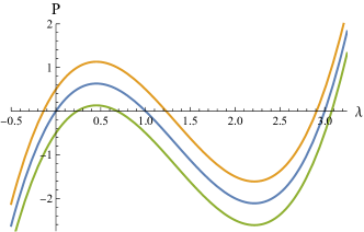
Figure 2: The cubic curve ${\tilde{P}}(\lambda)$ (the middle curve) and the cubics $P(\lambda)$ for $C>0$ (upper curve) and for $C<0$ (lower curve). The zero root of ${\tilde{P}}$ shifts to negative $\lambda$ for $C>0$ and to positive $\lambda$ for $C<0$. The root can become complex for sufficiently large and negative $C$.

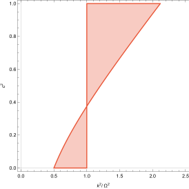
Figure 3: Stability plots for the TO modes for $\epsilon^{2}=\Omega^{2}/2$ (top), $\epsilon^{2}=\Omega^{2}$ (middle) and $\epsilon^{2}=3\Omega^{2}/2$ (bottom). As $\epsilon$ is decreased the two triangular regions in the $\epsilon^{2}<\Omega^{2}$ plot (top) shrink and approach the $k^{2}=\Omega^{2}$ vertical line as $\epsilon^{2}\to 0$.

Next let us return to the cubic in (41) which can be written as,

$$P(\lambda)={\tilde{P}}(\lambda)+C$$ (46)

where

$$C = -(k^{2}-\Omega^{2})[(k^{2}+\epsilon^{2}-\Omega^{2})(k^{2}+\epsilon^{2})-4\epsilon^{2}c^{2}k^{2}]$$ (47)

$$= -(\kappa-\Omega^{2})(\kappa-\kappa_{+})(\kappa-\kappa_{-})$$

where $\kappa\equiv k^{2}$,

$$\kappa_{\pm} = \frac{1}{2}\biggl{[}\Omega^{2}+2\epsilon^{2}c_{2}$$ (48)

$$\hskip 14.22636pt\pm\sqrt{\left(\Omega^{2}+2\epsilon^{2}c_{2}\right)^{2}-4\epsilon^{2}(\epsilon^{2}-\Omega^{2})}\ \biggr{]}$$

and $c_{2}\equiv\cos(2\theta)$. If $C>0$, the ${\tilde{P}}$ curve shifts upwards (see Fig. 2) and the $\lambda=0$ root of ${\tilde{P}}$ shifts to the left, i.e. $\lambda<0$. This indicates an instability. On the other hand, if $C<0$, there is no instability.

It is simplest to analyze the case with $\epsilon^{2}=\Omega^{2}$ for then

$$\kappa_{\pm}=\frac{\Omega^{2}}{2}\left[(4c^{2}-1)\pm|4c^{2}-1|\right]$$ (49)

For $c^{2}>1/4$, $\kappa_{-}=0$ and $\kappa_{+}=\Omega^{2}(4c^{2}-1)$. Then for $c^{2}>1/2$ we obtain an instability ($C>0$) for $\Omega^{2}<k^{2}<\Omega^{2}(4c^{2}-1)$ and for $1/4<c^{2}<1/2$ modes are unstable if $\Omega^{2}(4c^{2}-1)<k^{2}<\Omega^{2}$. For the opposite case of $c^{2}<1/4$, $\kappa_{-}=4c^{2}-1<0$ and $\kappa_{+}=0$. Then the instability occurs for $0<k^{2}<\Omega^{2}$. This explains the instability domains shown in Fig. 3 in the $\epsilon^{2}=\Omega^{2}$ case.

The analysis and results are similar for $\epsilon^{2}<\Omega^{2}$ as is clear from Fig. 3. With $c=0$, we find that $C>0$ for $\Omega^{2}-\epsilon^{2}<k^{2}<\Omega^{2}$. Essentially, as $\epsilon^{2}$ is reduced the domain of instability shrinks towards a vertical line along $k^{2}=\Omega^{2}$. An interesting limit is $\epsilon\to 0$ and $\Omega\to\infty$ with $\epsilon\Omega=E$ held constant. In this limit, there are no unstable TO modes.

The analysis is a bit more involved for $\epsilon^{2}>\Omega^{2}$. First consider $c^{2}=0$ ($c_{2}=-1$). Then (48) gives $\kappa_{\pm}=-\epsilon^{2},\,-\epsilon^{2}+\Omega^{2}$ and both roots are for negative $\kappa$. From (47) we then see that $C>0$ for $0<k^{2}<\Omega^{2}$ as is also seen in Fig. 3. Next consider $c^{2}=1$ ($c_{2}=+1$). Then (48) gives

$$\kappa_{\pm}=\frac{1}{2}\biggl{[}\Omega^{2}+2\epsilon^{2}\pm\sqrt{\Omega^{4}+8\epsilon^{2}\Omega^{2}}\ \biggr{]}.$$ (50)

Now $\kappa_{+}>\Omega^{2}$ but $\kappa_{-}$ may be larger or smaller than $\Omega^{2}$. If $\kappa_{-}<\Omega^{2}$, then from (47) we see that $C>0$ for $0<k^{2}<\kappa_{-}$ and also for $\Omega^{2}<k^{2}<\kappa_{+}$ but $C<0$ for $\kappa_{-}<k^{2}<\Omega^{2}$. Hence we see the gap in the instability domain in Fig. 3 at $c^{2}=1$. If, on the other hand, $\kappa_{-}>\Omega^{2}$, then $C>0$ for $0<k^{2}<\Omega^{2}$ and then again for $\kappa_{-}<k^{2}<\kappa_{+}$.

The shapes of the unstable regions can be understood in terms of the roots of $C$ in (47), namely 1 and $\kappa_{\pm}$. For example, in the case $\epsilon^{2}>\Omega^{2}$, for $c^{2}=0$, there is one real root ($\kappa=\Omega^{2}$) and $\kappa_{\pm}$ are negative. As $c^{2}$ increases, $\kappa_{\pm}$ become complex. At some critical value of $c^{2}$ the imaginary part of $\kappa_{\pm}$ vanishes. This is at the minimum of the parabolic shape in the plot of Fig. 3 and can occur for $k^{2}<\Omega^{2}$ or $k^{2}>\Omega^{2}$ depending on the value of $\epsilon^{2}/\Omega^{2}$. The left edge of the parabola is given by $\kappa_{-}$, and the right edge is given by $\kappa_{+}$. For yet larger $c^{2}$, $\kappa_{+}$ becomes larger than $\Omega^{2}$. The unstable region is when two of the factors in (47) are positive and one is negative.

VI TN and L modes ($\{\alpha_{a},\gamma_{a}\}$)

Eqs. 31-33 and 37-39 can be written in matrix form $MX=0$ with $X^{T}=(\alpha_{1},\alpha_{2},\alpha_{3},\gamma_{1},\gamma_{2},\gamma_{3})$ and

$$M=\begin{pmatrix}-\omega^{2}-\Omega^{2}&i2\omega\Omega&0&0&0&0\\ -i2\omega\Omega&-\omega^{2}-\Omega^{2}+\epsilon^{2}s^{2}&0&0&-\epsilon^{2}cs&i\epsilon sk\\ 0&0&-\omega^{2}+\epsilon^{2}s^{2}&0&-i\epsilon sk&-\epsilon^{2}cs\\ 0&0&0&-\omega^{2}+k^{2}-\Omega^{2}&i2\omega\Omega&0\\ 0&-\epsilon^{2}cs&i\epsilon sk&-i2\omega\Omega&-\omega^{2}+k^{2}-\Omega^{2}+\epsilon^{2}c^{2}&-i2\epsilon ck\\ 0&-i\epsilon sk&-\epsilon^{2}cs&0&i2\epsilon ck&-\omega^{2}+k^{2}+\epsilon^{2}c^{2}\end{pmatrix}$$ (51)

The eigenvectors are also required to satisfy the constraints in (28)-(30) as we will discuss further after considering some special cases.

VI.1 Special case: $c=1$

For $c=1$, the matrix in (51) becomes block diagonal in 3 blocks, the first is the $\{\alpha_{1},\alpha_{2}\}$ $2\times 2$ block with two degenerate eigenvalues $\omega^{2}=\Omega^{2}$, the second block is the $\{\alpha_{3}\}$ $1\times 1$ block with eigenvalue $\omega^{2}=0$, and the third $\{\gamma_{1},\gamma_{2},\gamma_{3}\}$ block is given by the matrix in (40) with $c=1$. Then the analysis in Sec. V for the TO modes applies immediately (with $c=1$). This is expected since for $c=1$ there is no distinction between TO and TN modes.

The constraint equations with $c=1$ read,

$$\omega k\alpha_{1}-i\Omega k\alpha_{2}+\epsilon\Omega\alpha_{3}=0$$ (52)

$$\omega k\alpha_{2}+i\Omega k\alpha_{1}-i\epsilon\omega\alpha_{3}=0$$ (53)

$$\omega k\alpha_{3}+i\epsilon\omega\alpha_{2}-2\epsilon\Omega\alpha_{1}=0$$ (54)

Note that the $\gamma_{a}$ are unconstrained. On the other hand, (52)-(54) over-constrain the eigensolutions in the $\{\alpha_{1},\alpha_{2}\}$ sector with $\omega=\pm\Omega$, and in the $\{\alpha_{3}\}$ sector with $\omega=0$, and neither of these two eigensolutions are physically admissible.

VI.2 Special case: $c=0$

With $c=0$, we have $s=1$, and the matrix in (51) becomes block diagonal in the $\{\alpha_{1},\alpha_{2},\gamma_{3}\}$ and the $\{\alpha_{3},\gamma_{1},\gamma_{2}\}$ blocks. The $3\times 3$ matrix for the first block is

$$M_{1}=\begin{pmatrix}-\omega^{2}-\Omega^{2}&i2\omega\Omega&0\\ -i2\omega\Omega&-\omega^{2}-\Omega^{2}+\epsilon^{2}&i\epsilon k\\ 0&-i\epsilon k&-\omega^{2}+k^{2}\end{pmatrix}$$ (55)

with constraint,

$$\omega k\alpha_{1}-i\Omega k\alpha_{2}+\epsilon\Omega\gamma_{3}=0$$ (56)

$$\omega k\alpha_{2}+i\Omega k\alpha_{1}-i\epsilon\omega\gamma_{3}=0$$ (57)

and the matrix for the second block is

$$\hskip-9.95863ptM_{2}=\begin{pmatrix}-\omega^{2}+\epsilon^{2}&0&-i\epsilon k\\ 0&-\omega^{2}+k^{2}-\Omega^{2}&i2\omega\Omega\\ i\epsilon k&-i2\omega\Omega&-\omega^{2}+k^{2}-\Omega^{2}\end{pmatrix}$$ (58)

with constraint,

$$\omega k\alpha_{3}+i\epsilon\omega\gamma_{2}-2\epsilon\Omega\gamma_{1}=0.$$ (59)

We now discuss these $3\times 3$ blocks separately.

VI.2.1 $\{\alpha_{1},\alpha_{2},\gamma_{3}\}$ block

In this block, gauge fields of the first two colors are oscillating in the longitudinal direction, whereas the third has amplitude in the transverse direction and orthogonal to the background electric field.

A straight-forward procedure would be to first solve the eigenproblem for $M_{1}$ and then check for the eigenvectors that satisfy the constraints. However we find it simpler to first solve the constraints (56)-(57) and then deal with the eigenproblem.

The constrains in (56)-(57) can be used to eliminate two of the three variables, say $\alpha_{2}$ and $\gamma_{3}$, while the third variable can be absorbed in the normalization of the resulting eigenvector. Hence we seek an eigenvector of the form,

$$V_{1}\equiv\begin{pmatrix}\alpha_{1}\\ \alpha_{2}\\ \gamma_{3}\end{pmatrix}=\begin{pmatrix}2\epsilon\omega\Omega\\ -i\epsilon(\omega^{2}+\Omega^{2})\\ k(-\omega^{2}+\Omega^{2})\end{pmatrix}$$ (60)

Insertion in $M_{1}V_{1}=0$ shows that there is no solution for $\omega$ for $\epsilon\neq 0$, $k\neq 0$. Hence these modes are over-constrained and absent. For $k=0$, $M_{1}V_{1}=0$ gives

$$(\omega^{2}-\Omega^{2})^{2}-\epsilon^{2}(\omega^{2}+\Omega^{2})=0$$ (61)

which has the roots

$$\omega_{\pm}^{2}=\Omega^{2}+\frac{\epsilon^{2}}{2}\pm\sqrt{\left(\Omega^{2}+\frac{\epsilon^{2}}{2}\right)^{2}+\Omega^{2}(\epsilon^{2}-\Omega^{2})}$$ (62)

Therefore $\omega_{-}^{2}<0$ if and only if $\Omega^{2}<\epsilon^{2}$ and $k=0$.

VI.2.2 $\{\alpha_{3},\gamma_{1},\gamma_{2}\}$ block

In this block, the gauge field of the third color oscillates in the longitudinal direction, whereas the first two colors oscillate transversely and orthogonal to the background electric field.

Now the constraint (59) reduces the eigenvector to be of the form,

$$V_{2}\equiv\begin{pmatrix}\alpha_{3}\\ \gamma_{1}\\ \gamma_{2}\end{pmatrix}=\begin{pmatrix}2\epsilon\Omega\alpha_{3}\\ \omega(k\alpha_{3}+i\epsilon\gamma_{2})\\ 2\epsilon\Omega\gamma_{2}\end{pmatrix}.$$ (63)

Imposing $M_{2}V_{2}=0$ we find the solution $\omega^{2}=\epsilon^{2}$ provided $k^{2}=\epsilon^{2}+\Omega^{2}$, and this mode is stable. For $k=0$ there is a solution with $\omega^{2}=\epsilon^{2}$.

An unusual feature of the first of these two modes is that it has non-trivial spatial dependence but it exists only for a fixed value of $k=\sqrt{\epsilon^{2}+\Omega^{2}}$ and the direction of ${\bf k}$ is perpendicular to the electric field, while the mode is polarized along the electric field and in the longitudinal direction. This mode represents fluctuations in the homogeneity of the electric field but with a definite wavelength.

VI.3 Special case: $k^{2}\gg\Omega^{2},\epsilon^{2}$

We now consider the ultraviolet limit $k^{2}\gg\Omega^{2},\epsilon^{2}$. The constraints (28)-(30) now give

$$\alpha_{1}=0=\alpha_{2}=\alpha_{3}$$ (64)

and only the $\{\gamma_{a}\}$ represent physical modes with the dispersion relation $\omega^{2}=k^{2}$. There are no unstable modes in this limit.

VI.4 Special case: $k\to 0$

The problem simplifies in the $k\to 0$ limit as the $\{\alpha_{3},\gamma_{3}\}$ block decouples from the $\{\alpha_{1},\alpha_{2},\gamma_{1},\gamma_{2}\}$ block.

The $2\times 2$ matrix for the $\{\alpha_{3},\gamma_{3}\}$ block is

$$M_{3}=\begin{pmatrix}-\omega^{2}+\epsilon^{2}s^{2}&-\epsilon^{2}cs\\ -\epsilon^{2}cs&-\omega^{2}+\epsilon^{2}c^{2}\end{pmatrix}$$ (65)

and the constraint reduces to $c\alpha_{3}+s\gamma_{3}=0$. $M_{3}$ has eigenvalues $\omega^{2}=0$ and $\omega^{2}=\epsilon^{2}$ but only the latter is consistent with the constraint. Thus there are no unstable modes in the $\{\alpha_{3},\gamma_{3}\}$ block.

The $4\times 4$ matrix for the $\{\alpha_{1},\alpha_{2},\gamma_{1},\gamma_{2}\}$ block is

$$M_{4}=\begin{pmatrix}-\omega^{2}-\Omega^{2}&i2\omega\Omega&0&0\\ -i2\omega\Omega&-\omega^{2}-\Omega^{2}+\epsilon^{2}s^{2}&0&-\epsilon^{2}cs\\ 0&0&-\omega^{2}-\Omega^{2}&i2\omega\Omega\\ 0&-\epsilon^{2}cs&-i2\omega\Omega&-\omega^{2}-\Omega^{2}+\epsilon^{2}c^{2}\end{pmatrix}$$ (66)

and the constraint is

$$i\omega(c\alpha_{2}+s\gamma_{2})-2\Omega(c\alpha_{1}+s\gamma_{1})=0.$$ (67)

We solve (31) and (37) with $k=0$ to get

$$\alpha_{2}=-i\frac{(\omega^{2}+\Omega^{2})}{2\omega\Omega}\alpha_{1},\ \ \gamma_{2}=-i\frac{(\omega^{2}+\Omega^{2})}{2\omega\Omega}\gamma_{1},$$ (68)

which, together with (67), gives

$$(\omega^{2}-3\Omega^{2})(c\alpha_{1}+s\gamma_{1})=0.$$ (69)

Therefore to satisfy the constraint we must either have $\omega^{2}=3\Omega^{2}>0$ or $c\alpha_{1}+s\gamma_{1}=0$.

Evaluation of the determinant of $M_{4}$ on Mathematica gives,

$${\rm Det}(M_{4})=(\omega^{2}-\Omega^{2})^{2}[(\omega^{2}-\Omega^{2})^{2}-\epsilon^{2}(\omega^{2}+\Omega^{2})]$$ (70)

This has the root $\omega^{2}=3\Omega^{2}$ but only if $\Omega^{2}=\epsilon^{2}$. In any case, $\omega^{2}=3\Omega^{2}>0$ and implies a stable mode. So we now focus on the other case, namely

$$c\alpha_{1}+s\gamma_{1}=0.$$ (71)

Combining (71) with (68), and ignoring an overall normalization factor, the Gauss constraint forces us to only consider the eigenvector,

$$\hskip-5.69046ptV_{4}^{T}=\left(2\omega\Omega s,-i{(\omega^{2}+\Omega^{2})}s,-2\omega\Omega c,i{(\omega^{2}+\Omega^{2})}c\right).$$ (72)

Requiring $M_{4}V_{4}=0$ leads once again to (61) and to the roots in (62). Therefore $\omega_{-}^{2}<0$ if and only if $\Omega^{2}<\epsilon^{2}$ and $k=0$ and the unstable eigenmode can be found by setting $\omega=\omega_{-}$ in (72).

VI.5 Special case: $\Omega=E/\epsilon$, $\epsilon\to 0$

In Sec. V we have seen that there are no unstable TO modes with $\Omega=E/\epsilon$ and $\epsilon\to 0$. Now we consider the TN and L modes in this regime.

With $\epsilon\to 0$, the matrix $M$ in (51) takes on a simple block diagonal form. The $\{\alpha_{1},\alpha_{2}\}$ block has two degenerate eigenvalues $\omega^{2}=\Omega^{2}$; the $\{\alpha_{3}\}$ block has eigenvalue $\omega^{2}=0$; the $\{\gamma_{1},\gamma_{2}\}$ block has eigenvalues $\omega^{2}=(k\pm\Omega)^{2}$; and the $\{\gamma_{3}\}$ block has eigenvalue $\omega^{2}=k^{2}$. The corresponding eigenvectors can be inserted into equations (28)-(30) to check if the Gauss constraints are satisfied. However, since none of the eigenvalues for $\omega^{2}$ are negative, it is clear that there are no unstable TN and L modes for these limiting parameters.

VII Conclusions

We have considered the stability of a homogeneous electric field background in pure SU(2) gauge theory. The gauge fields underlying the electric field are taken to be of the form in (5) and not of the Maxwell type: $A_{i}^{a}=-Et\delta^{a3}\delta_{iz}$. This is because gauge fields of the Maxwell type are unstable to Schwinger pair production while the gauge fields in (5) are protected from decay due to this process Vachaspati (2022). However, the gauge fields in (5) are not solutions of the vacuum classical equations of motion; instead non-vanishing currents are necessary. There are two ways to explain these non-vanishing currents. The first is that they are due to classical external sources in which case they are simply postulated. The second way is that the classical equations of motion should be replaced by equations that take quantum effects into account and these “effective classical equations” can contain sources. For example, in the semiclassical approximation quantum fluctuations provide current sources for the background Vachaspati (2022),

$$j^{\mu a} \equiv \epsilon^{abc}\langle\partial_{\nu}q^{\nu b}q^{\mu c}-q^{\nu b}\partial^{\mu}q_{\nu}^{c}+2q^{\nu b}\partial_{\nu}q^{\mu c}\rangle_{R}$$ (73)

$$+A_{\nu}^{b}\langle q^{\nu a}q^{\mu b}-2q^{\nu b}q^{\mu a}\rangle_{R}+A_{\nu}^{a}\langle q^{\nu b}q^{\mu b}\rangle_{R}$$

$$+A^{\mu b}\langle q^{b}_{\nu}q^{\nu a}\rangle_{R}-A^{\mu a}\langle q_{\nu}^{b}q^{\nu b}\rangle_{R}$$

where $q^{a}_{\mu}$ are the quantum fluctuations in the background $A^{a}_{\mu}$ and $\langle\cdot\rangle_{R}$ denotes a renormalized expectation value taken in the quantum state of $q^{a}_{\mu}$. For stable modes, the quantum state might be given by simple harmonic oscillator states for each of the eigenmodes of $q^{a}_{\mu}$. However the quantum state of unstable modes will not be simple harmonic oscillator states which is why it is important to perform a stability analysis. We will comment further on the unstable modes after summarizing our results.

The gauge field background in (5) is described by two parameters: $\epsilon$ and $\Omega$. The electric field strength is given by $E=\epsilon\Omega$. The results of the fluctuation analysis depend on whether $\epsilon^{2}>\Omega^{2}$ or $\epsilon^{2}\leq\Omega^{2}$. The fluctuations naturally split into “TO modes”” that are transverse to the wavevector ${\bf k}$ and orthogonal to the background electric field, “TN modes” that are transverse to ${\bf k}$ but not orthogonal to the electric field, and “L modes” that are in the longitudinal direction.

The TO modes decouple from the TN and L modes. The stability analysis of Sec. V shows that TO modes are stable except in a range of $k^{2}$ that depends on the angle $\theta$ between the electric field and the wavevector ${\bf k}$. The instability regions depend on the background parameters and are plotted in Fig. 3. There are two important results emerging from our analysis. The first is that the region of parameter space $(k^{2},c^{2})$ ($c=\cos\theta$) where unstable modes exist depends on the relation between $\epsilon^{2}$ and $\Omega^{2}$. The instability region is smaller when $\epsilon^{2}<\Omega^{2}$ and shrinks to zero as $\epsilon^{2}\to 0$. Note that the electric field strength is given by $E=\epsilon\Omega$ and can be held fixed in the limit by also taking $\Omega\to\infty$. The second is that unstable modes exist only for small values of $k^{2}$. For example, for $\epsilon=\Omega$, there are no unstable modes for $k^{2}>3\epsilon^{2}$ for any value of $c^{2}$.

The TN and L modes are coupled in general and the analysis is more involved than for the TO modes. In Sec. VI we discuss the stability of these modes in various parameter regimes. The special cases of $\theta=0$ and $\theta=\pi/2$ are considered. For $\theta=0$ the analysis is identical to that of TO modes, while for $\theta=\pi/2$ there is an instability if $\epsilon^{2}>\Omega^{2}$ and $k=0$. There is also a special stable mode that corresponds to oscillations of the background electric field orthogonal to its direction, similar to a sound wave. We have also considered the special case of large $k^{2}$ and here the modes are simply those of free massless waves with dispersion $\omega^{2}=k^{2}$. Finally, we examine the $\epsilon\to 0$ limit with $E=\epsilon\Omega$ held fixed and show that there are no unstable TN and L modes, just as there are no unstable TO modes in this limit.

As mentioned in Sec. I, we were motivated to perform this stability analysis because confining strings in QCD are expected to be stable. The electric fields we have considered as backgrounds do not excite Schwinger pair production but, as we have seen, have classical instabilities for certain infrared modes. How do these classical instabilities impact the possibility that the electric fields we have considered are responsible for confining strings? The first point we note is that there are no instabilities in the limit of $\epsilon\to 0$ and $E=\epsilon\Omega$ fixed. So it could be that the electric field in a confining string corresponds to this set of parameters. Then there are no unstable modes and the quantum state for each mode is that of a simple harmonic oscillator. The second point is that the instabilities we have found are for a homogeneous electric field and only occur for small values of $k^{2}$, ($k^{2}\lesssim\epsilon^{2}$ for $\epsilon^{2}>\Omega^{2}$) that is, on large length scales. In contrast, the electric flux in a string only has support in a finite area – the string cross-section – and we do not expect any unstable modes on length scales larger than the thickness of the string. (Though there is still the question of the infinite extent of the string along the electric field direction and whether the instabilities for $\theta=0$ will survive.) It would be worthwhile performing an explicit stability analysis for a flux tube configuration such as Vachaspati (2022),

$$A^{\pm}_{\mu}=-\epsilon e^{\pm i\Omega t}\,f(r)\,\partial_{\mu}z,\ \ A^{3}_{\mu}=0,$$ (74)

where $f(r)$ is a profile function for the string and $r\equiv\sqrt{x^{2}+y^{2}}$ is the cylindrical radial coordinate. Another interesting question is if the homogeneous electric field background we have considered is unstable towards forming an Abrikosov lattice Abrikosov (1957) of electric flux tubes. After all we have identified certain unstable modes with spatial dependence that is orthogonal to the background homogeneous electric field.