Mapping Slightly Broken Higher Spin (SBHS) theory correlators to Free theory correlators: A momentum space bootstrap using SBHS symmetry

Abstract

We develop a systematic method to constrain any n-point correlation function of spinning operators in Slightly Broken Higher Spin (SBHS) theories. As an illustration of the methodology, we work out the three point functions which reproduce the previously known results. We then work out the four point functions of spinning operators. We show that the correlation functions of spinning operators in the interacting SBHS theory take a remarkably simple form and that they can be written just in terms of the free fermionic and critical bosonic theory correlators. They also interpolate nicely between the results in these two theories. When expressed in spinor-helicity variables we obtain an anyonic phase which nicely interpolates between the free fermionic and critical bosonic results which makes 3D bosonization manifest.

Assuming a form of the five point scalar correlator, we also work out several five point functions to illustrate how our method can be used in five or higher point functions. We also put forth a conjecture for any n-point function of spinning operators in SBHS theories. In this paper we have bootstrapped correlators using SBHS symmetry in momentum space and spinor helicity variables. In general, solving the SBHS constraints are complicated to analyse in position space, but in momentum space and spinor-helicity variables they can be solved efficiently and this is greatly helped by the recent development of momentum space CFT correlation functions.

1 Introduction

Bootstrapping is an important idea which enables us to compute physical quantities of interest based on symmetries and general considerations without requiring much of the microscopic details of the theory. Recently, the conformal bootstrap programme Rychkov:2016iqz ; Poland:2022qrs ; Hartman:2022zik and S-matrix bootstrap Kruczenski:2022lot have played a significant role in our understanding of conformal field theory as well as quantum field theories in general. The conformal bootstrap programme has been developed mainly in position space and in Mellin space Gopakumar:2016wkt . The S-matrix bootstrap, on the other hand is naturally developed in momentum space. These two programmes have been developed independently without much overlap. One possible way to bridge this gap is by studying conformal field theory in momentum space. Momentum space CFT analysis is important as it plays an important role in the context of cosmological correlation functions Maldacena:2011nz , in condensed matter physics applications, its connection to one higher dimensional amplitudes in curved space and the flat space S-matrix Maldacena:2011nz ; Penedones:2010ue ; Raju:2012zr . Even though it is important to understand CFT correlation functions in momentum space, there exist very limited results. Maldacena:2011nz ; Coriano:2013jba ; Bzowski:2013sza ; Bzowski:2015pba ; Bzowski:2017poo ; Bzowski:2018fql ; Kundu:2014gxa ; Pajer:2020wxk ; Gillioz:2019lgs ; Isono:2019ihz ; Baumann:2019oyu ; Jain:2020rmw ; Jain:2020puw ; Jain:2021wyn ; Jain:2021vrv ; Caron-Huot:2021kjy ; Jain:2021gwa ; Gandhi:2021gwn .

One of the reasons why conformal field theory in momentum space has got very limited attention is its technical difficulty even at the level of the three point functions. One can also ask, what new things might one learn by thinking in Fourier space? As has been established in recent developments, at least in three dimensions, momentum space analysis has already led to interesting new insights into the structure of CFT correlators Farrow:2018yni ; Caron-Huot:2021kjy ; Jain:2021vrv ; Jain:2021qcl ; Jain:2021gwa ; Gandhi:2021gwn ; Jain:2021whr . In an early work Giombi:2011rz ; Maldacena:2012sf by performing a position space analysis, it was shown that the three point functions of conserved currents in three dimensions generally have three structures which are the free bosonic, the free fermionic and a parity odd part which can’t be obtained from the free theories. However momentum space analysis revealed that the parity odd part can be obtained by a simple transformation Jain:2021gwa of the parity even part. Further it was shown that all three different structures can be constructed just from the free bosonic or just the free fermionic theory results Jain:2021whr . Even though the computation of the three point functions has seen some progress, very limited results exist for four point functions. There has been a lack of systematic analysis of four point CFT correlation functions and all the more less for spinning ones. Any development of the four point functions would be very useful. In this paper we consider a particular class of CFTs, the slightly broken higher spin theories Maldacena:2012sf ; Giombi:2011kc ; Aharony:2011jz . We constrain the form of the four point and five point functions and make a conjecture for n point functions of spinning operators for slightly broken HS theories using momentum space or spinor helicity considerations. We show that the momentum space considerations are particularly useful in the context of theories with slightly broken Higher Spin symmetries.

Examples of slightly broken higher spin theories are given by Chern-Simons matter theories at large N. Chern-Simons gauge field coupled to matter in the fundamental representation has been the subject of intense research in the recent past Sezgin:2002rt ; Klebanov:2002ja ; Giombi:2009wh ; Benini:2011mf ; Giombi:2011kc ; Aharony:2011jz ; Maldacena:2011jn ; Maldacena:2012sf ; Chang:2012kt ; Jain:2012qi ; Aharony:2012nh ; Yokoyama:2012fa ; GurAri:2012is ; Aharony:2012ns ; Jain:2013py ; Takimi:2013zca ; Jain:2013gza ; Yokoyama:2013pxa ; Jain:2014nza ; Gurucharan:2014cva ; Bardeen:2014qua ; Bardeen:2014paa ; Dandekar:2014era ; Frishman:2014cma ; Moshe:2014bja ; Aharony:2015pla ; Inbasekar:2015tsa ; Bedhotiya:2015uga ; Minwalla:2015sca ; Gur-Ari:2015pca ; Radicevic:2015yla ; Geracie:2015drf ; Aharony:2015mjs ; Radicevic:2016wqn ; Karch:2016sxi ; Hsin:2016blu ; Yokoyama:2016sbx ; Gur-Ari:2016xff ; Murugan:2016zal ; Seiberg:2016gmd ; Giombi:2016ejx ; Karch:2016aux ; Giombi:2016zwa ; Wadia:2016zpd ; Aharony:2016jvv ; Giombi:2017rhm ; Charan:2017jyc ; Benini:2017dus ; Sezgin:2017jgm ; Nosaka:2017ohr ; Komargodski:2017keh ; Giombi:2017txg ; Gaiotto:2017tne ; Jensen:2017dso ; Jensen:2017xbs ; Inbasekar:2020hla ; Gomis:2017ixy ; Inbasekar:2017ieo ; Inbasekar:2017sqp ; Cordova:2017vab ; Benini:2017aed ; Aitken:2017nfd ; Jensen:2017bjo ; Karch:2018mer ; Chattopadhyay:2018wkp ; Turiaci:2018nua ; Choudhury:2018iwf ; Aharony:2018npf ; Yacoby:2018yvy ; Aitken:2018cvh ; Aharony:2018pjn ; Dey:2018ykx ; Chattopadhyay:2019lpr ; Dey:2019ihe ; Halder:2019foo ; Aharony:2019mbc ; Li:2019twz ; Jain:2019fja ; Inbasekar:2019wdw ; Inbasekar:2019azv ; Jensen:2019mga ; Kalloor:2019xjb ; Ghosh:2019sqf ; Jain:2020rmw ; Minwalla:2020ysu ; Jain:2020puw ; Mishra:2020wos ; Minwalla:2022sef ; Jain:2022izp . These are interesting models as several large-N exact computations can be performed, they show strong weak field theory/field theory duality which are called Bose-Fermi dualities. These theories also provide a concrete example of non super symmetric Gauge/Gravity duality. Several exact computation suggest that these theories may be integrable. In the context of correlation functions of spinning operators, direct perturbative computations have been done for a few three and four point functions in a special kinemetic regime Aharony:2012nh ; GurAri:2012is ; Bedhotiya:2015uga ; Turiaci:2018nua ; Kalloor:2019xjb . Recently, using purely conformal field theory arguments it was shown that in spinor helicity variables that the three point functions of spinning operators take on a very interesting form and appear to have an anyonic phase Gandhi:2021gwn which was earlier observed in the context of $2\rightarrow 2$ scattering. Since three point functions are universal and are completely fixed by conformal symmetry, we required hardly any input from the Chern-Simons matter theories. However at the level of the four point functions, any such results would require a lot more information from the specific theory at hand . At the level of the three point functions, in Maldacena:2011jn ; Maldacena:2012sf slightly broken HS symmetry was used to constrain the three point functions in these theories. Subsequently, in Li:2019twz ; Jain:2020rmw ; Jain:2020puw ; Silva:2021ece , four point correlation functions of the form $\langle J_{s}OOO\rangle$ were explored. In this paper, we develop a methodology to solve slightly broken HS equations which in principle can be used to solve any n-point function of spinning operators in terms of the free theory correlators.

The rest of the paper is organised as follows:
In section 2, we briefly describe the theory that we shall be interested in. In section 3 we briefly review and summarise the answers that we obtain in this paper. Section 4 describes a flowchart that we use in the rest of the paper to solve slightly broken HS theories. In section 5, we demonstrate our methodology with the help of several examples of three point functions and reproduce known results. In section 6 we solve the four point functions. Then, in section 7 we solve for a particular five point function to illustrate our methodology in the five point case (further supplemented by more examples in H). In section 8 we describe how the WT identity for slightly broken HS theory can be understood in terms of the free theory WT identities. This also suggests that slightly broken HS algebra can be understood in terms of the free theory HS algebra. We explore this in one of the appendices. In section 9 we summarize our results and discuss various future directions. We also have several appendices which are useful for our main text.

2 CS Matter theories: A short summary

Here we will briefly review Chern-Simons matter theories. There are two classes of these theories, namely the Quasi fermion (QF) and the Quasi bosonic theories. In this work, we mainly deal with the QF theory. The details of these theories can be found for example in Aharony:2018pjn .

2.1 Quasi Fermionic theory

Quasi fermionic theory refers to two different theories, namely CS gauge field coupled to a fermion or CS gauge field coupled to a critical boson. We review this below.

Fermionic theory coupled to CS field

The fermionic theory coupled to $SU(N_{f})$ Chern-Simons gauge field has the following action

$$S=\int d^{3}x\left[\bar{\psi}\gamma_{\mu}D^{\mu}\psi+i\epsilon^{\mu\nu\rho}\frac{\kappa_{f}}{4\pi}\text{Tr}(A_{\mu}\partial_{\nu}A_{\rho}-\frac{2i}{3}A_{\mu}A_{\nu}A_{\rho})\right]$$ (1)

We are interested in the limit as $N_{f}\rightarrow\infty$ and $\kappa_{f}\rightarrow\infty$ such that $\lambda_{f}=\frac{N_{f}}{\kappa_{f}}$ is held fixed. The spectrum of operators consists of exactly conserved spin 1 and spin 2 currents and in general spin-s currents $J_{s}$ with scaling dimensions $\Delta_{s}=s+1+{\mathcal{O}}(\frac{1}{N_{f}})$ for $s\geq 3$. The scalar operator has conformal dimension $\Delta=2+\mathcal{O}\left(\frac{1}{N_{f}}\right)$ and is parity odd.

Critical bosonic theory coupled to Chern-Simons theory in $d=3$

Let us consider the critical bosonic theory coupled to Chern-Simons $SU(N_{b})$ gauge field. The critical theory is obtained by adding an interaction of the kind $\sigma_{b}\bar{\phi}\phi$ where $\sigma_{b}$ is an auxiliary field to the free bosonic Lagrangian. The theory has the following action

$$S=\int d^{3}x\left[D_{\mu}\bar{\phi}D^{\mu}\phi+i\epsilon^{\mu\nu\rho}\frac{\kappa_{b}}{4\pi}\text{Tr}(A_{\mu}\partial_{\nu}A_{\rho}-\frac{2i}{3}A_{\mu}A_{\nu}A_{\rho})+\sigma_{b}\bar{\phi}\phi\right]$$ (2)

Again, we are interested in the limit as $N_{b}\rightarrow\infty$ and $\kappa_{b}\rightarrow\infty$ such that $\lambda_{b}=\frac{N_{b}}{\kappa_{b}}$ is held fixed. The spin-1 and spin-2 conserved currents have scaling dimensions 2 and 3 respectively. Apart from these, there is an infinite tower of slightly broken higher spin currents. The conformal dimension of the spin $s$ current $\Delta=s+1+\mathcal{O}\left(\frac{1}{N}\right)$. The scalar operator has conformal dimension $\Delta=2+\mathcal{O}(\frac{1}{N})$ and is parity even.

2.2 Slightly broken Higher spin symmetry

The free theories have exactly conserved higher spin currents $\partial.J_{s}=0$ for all s. For CS matter theories, we have currents which are not exactly conserved, that is $\partial.J_{s}\neq 0$ for $s>2.$ In this paper we are going to use these symmetries to constrain the form of correlation functions of arbitrary spinning operators following Maldacena:2011jn ; Maldacena:2012sf . More precisely we are going to use

$$\sum_{i=1}^{n}\langle J_{s_{1}}(x_{1})\ldots[Q_{s},J_{s_{i}}(x_{i})]\ldots J_{s_{n}}(x_{n})\rangle=\int_{x}\langle\partial.J_{s}(x)J_{s_{1}}(x_{1})\ldots J_{s_{i}}(x_{i})\ldots J_{s_{n}}(x_{n})\rangle$$ (3)

where $Q_{s}$ is the charge associated with current $J_{s}$ and $\partial.J_{s}(x)\neq 0$. A more detailed form will be discussed in the subsequent sections. In this paper following Maldacena:2012sf we shall use (3) to solve for the correlation functions.

Some useful definitions

The coupling constant in the CS gauge field coupled to a fermion in the limit $N_{f}\rightarrow\infty,\kappa_{f}\rightarrow\infty,$ is defined as follows,

$$\lambda_{f}=\frac{N_{f}}{\kappa_{f}}$$ (4)

We now introduce a few other useful variables which will help simplify our expressions Aharony:2012nh ; GurAri:2012is

$$\tilde{N}=2N_{f}\frac{\sin\pi\lambda_{f}}{\pi\lambda_{f}},\quad\tilde{\lambda}=\tan\left(\frac{\pi\lambda_{f}}{2}\right)$$ (5)

In the main text we will be working only in the quasi-fermionic theory. In some normalisation we can fix $\lambda_{f}$ to take values $0\leq\lambda_{f}\leq 1.$ We discuss the Quasi Bosonic theory in appendix A . We will also frequently use the abbreviations listed in the table below:

Abbreviation	Full Form
SBHS	Slightly broken higher spin
HSE	Higher spin equation
FB	Free Boson
FF	Free Fermion
CB	Critical Boson
CF	Critical Fermion
QB	Quasi Boson
QF	Quasi Fermion

Table 1: Abbreviations

3 Summary of results

In this section we summarise the results we have obtained in this paper. Let us describe some of the notation that is going to be useful.

Notation

Here we introduce some notation for the correlators which we will use to state our results. For any correlator we define

Notation	Description
$\langle...\rangle_{\text{QF}}$	In quasi-fermionic theory
$\langle...\rangle_{\text{FF/FB}}$	In free fermionic/bosonic theory
$\langle...\rangle_{\text{CB}}$	In critical bosonic theory
$\langle...\rangle_{\text{odd}}$	Parity odd correlator
$\langle...\rangle_{\text{FF+FB}}$	$\langle...\rangle_{\text{FF}}+\langle...\rangle_{\text{FB}}$
$\langle...\rangle_{\text{FF-FB}}$	$\langle...\rangle_{\text{FF}}-\langle...\rangle_{\text{FB}}$

Table 2: Notation for correlators

Epsilon transform

We will also be using an operation known as the epsilon transform very frequently. We denote the epsilon transform D of $X$ as $\epsilon\cdot X$. The epsilon transform maps a parity even/odd correlation function to a parity odd/even correlator Caron-Huot:2021kjy ; Jain:2021gwa . We also make the following useful definition where,

$$\epsilon\cdot X_{\mu\alpha_{1}...\alpha_{n}}=\frac{\epsilon_{\mu ab}p_{a}}{p}X_{b\alpha_{1}...\alpha_{n}}$$ (7)

In position space, the epsilon transform is defined as Caron-Huot:2021kjy ; Jain:2021gwa

$$\langle\epsilon.J^{\mu_{1}\mu_{2}\cdots\mu_{s_{1}}}(y_{1})J_{s_{2}}(y_{2})J_{s_{3}}(y_{3})\rangle=\epsilon^{(\mu_{1}}_{\sigma\alpha}\int\frac{d^{3}x_{1}}{|y_{1}-x_{1}|^{2}}~{}~{}\partial_{x_{1}}^{\sigma}\langle J^{\alpha\mu_{2}\cdots\mu_{s_{1}})}(x_{1})J_{s_{2}}(y_{2})J_{s_{3}}(y_{3})\rangle$$ (8)

In momentum space the relation is simpler and can be written as Jain:2021gwa

$$\langle\epsilon.J^{\mu_{1}\mu_{2}\cdots\mu_{s_{1}}}(p_{1})J_{s_{2}}(p_{2})J_{s_{3}}(p_{3})\rangle=\frac{1}{p_{1}}\epsilon^{\mu_{1}\alpha p_{1}}\langle J_{\alpha}^{\mu_{2}\cdots\mu_{s_{1}}}(p_{1})J^{\nu_{1}\cdots\nu_{s_{2}}}(p_{2})J^{\rho_{1}\cdots\rho_{s_{3}}}(p_{3})\rangle+ (\mu_{1}\leftrightarrow\mu_{2})+\cdots+(\mu_{1}\leftrightarrow\mu_{s_{1}})$$ (9)

Converting to spinor helicity variables Jain:2021vrv ; Jain:2021gwa , $\langle\epsilon\cdot J_{s_{1}}J_{s_{2}}J_{s_{3}}\rangle$ becomes $\pm i\langle J_{s_{1}}J_{s_{2}}J_{s_{3}}\rangle$ depending on the helicity.

Having discussed various notations, let us now summarise the results in this paper. To do that we first summarise the known two and three point functions and then we come to the four point functions.

3.1 2 point function

We write the general two point function as,

$$\langle J_{s}J_{s}\rangle_{\text{QF}}=\tilde{N}\langle J_{s}J_{s}\rangle_{\text{FF}}+\tilde{N}\tilde{\lambda}\langle J_{s}J_{s}\rangle_{\text{odd}}$$ (10)

It can be shown that Caron-Huot:2021kjy ; Jain:2021gwa the parity odd part can be written in terms of the parity even part and it turns out that

$$\langle J_{s}J_{s}\rangle_{\text{QF}}=\tilde{N}\langle J_{s}J_{s}\rangle_{\text{FF}}+\tilde{N}\tilde{\lambda}\langle\epsilon\cdot J_{s}J_{s}\rangle_{\text{FF}}$$ (11)

which upon converting to spinor helicity variables gives, Gandhi:2021gwn

$$\langle J_{s}^{-}J_{s}^{-}\rangle_{QF}=\frac{Ne^{i\pi\lambda_{f}}}{\pi\lambda_{f}}\langle J_{s}^{-}J_{s}^{-}\rangle_{FF}$$ (12)

where we have used (5).

3.2 3-point functions

It was shown in Maldacena:2012sf that for the case of three point functions in the quasi fermionic theory we have

$$\langle J_{s}OO\rangle_{\text{QF}} =\tilde{N}(1+\tilde{\lambda}^{2})\langle J_{s}OO\rangle_{\text{FF}}$$

$$\langle J_{s_{1}}J_{s_{2}}O\rangle_{\text{QF}} =\tilde{N}\langle J_{s_{1}}J_{s_{2}}O\rangle_{\text{FF}}+\tilde{N}\tilde{\lambda}\langle J_{s_{1}}J_{s_{2}}O\rangle_{\text{CB}}$$

$$\langle J_{s_{1}}J_{s_{2}}J_{s_{3}}\rangle_{\text{QF}} =\frac{\tilde{N}}{1+\tilde{\lambda}^{2}}\bigg{[}\langle J_{s_{1}}J_{s_{2}}J_{s_{3}}\rangle_{\text{FF}}+\tilde{\lambda}\langle J_{s_{1}}J_{s_{2}}J_{s_{3}}\rangle_{\text{odd}}+\tilde{\lambda}^{2}\langle J_{s_{1}}J_{s_{2}}J_{s_{3}}\rangle_{\text{FB}}\bigg{]}$$ (13)

In the above expression the momentum labels and the indices have been suppressed for clarity and they can be restored appropriately.

However, it was realized Jain:2021gwa that we can write the odd piece in terms of the FF and FB correlators and the final answer turns out to be

$$\langle J_{s_{1}}OO\rangle_{\text{QF}} =\tilde{N}(1+\tilde{\lambda}^{2})\langle J_{s_{1}}OO\rangle_{\text{FF}}$$

$$\langle J_{s_{1}}J_{s_{2}}O\rangle_{\text{QF}} =\tilde{N}\langle J_{s_{1}}J_{s_{2}}O\rangle_{\text{FF}}+\tilde{N}\tilde{\lambda}\langle\epsilon\cdot J_{s_{1}}J_{s_{2}}O\rangle_{\text{FF}}$$

$$\langle J_{s_{1}}J_{s_{2}}J_{s_{3}}\rangle_{\text{QF}} =\frac{\tilde{N}}{1+\tilde{\lambda}^{2}}\bigg{[}\langle J_{s_{1}}J_{s_{2}}J_{s_{3}}\rangle_{\text{FF}}+\tilde{\lambda}\langle\epsilon\cdot J_{s_{1}}J_{s_{2}}J_{s_{3}}\rangle_{\text{FF-FB}}+\tilde{\lambda}^{2}\langle J_{s_{1}}J_{s_{2}}J_{s_{3}}\rangle_{\text{FB}}\bigg{]}$$ (14)

We now convert the last equation of (3.2) to spinor helicity variables. For brevity we will work with all helicities as minus. In all minus helicity we have $\langle\epsilon\cdot J_{s_{1}}J_{s_{2}}J_{s_{3}}\rangle_{\text{FF-FB}}=i\langle J_{s_{1}}J_{s_{2}}J_{s_{3}}\rangle_{\text{FF-FB}}$.

Then combining the FF and FB terms, and substituting $\tilde{\lambda}=\tan{\frac{\pi\lambda_{f}}{2}}$ we get,

$$\langle J_{s_{1}}J_{s_{2}}J_{s_{3}}\rangle_{\text{QF}}= \frac{\tilde{N}}{2}\bigg{[}\langle J_{s_{1}}J_{s_{2}}J_{s_{3}}\rangle_{\text{FF+FB}}+e^{-i\pi\lambda_{f}}\langle J_{s_{1}}J_{s_{2}}J_{s_{3}}\rangle_{\text{FF-FB}}\bigg{]}$$

$$= \tilde{N}e^{-\frac{i\pi\lambda_{f}}{2}}\bigg{[}\cos{\frac{\pi\lambda_{f}}{2}}\langle J_{s_{1}}J_{s_{2}}J_{s_{3}}\rangle_{\text{FF}}+i\sin{\frac{\pi\lambda_{f}}{2}}\langle J_{s_{1}}J_{s_{2}}J_{s_{3}}\rangle_{\text{FB}}\bigg{]}$$ (15)

For, $\lambda_{f}=0$, we get the FF correlator and for $\lambda_{f}=1$, we get the FB correlator.

3-point functions in terms of homogeneous and non-homogeneous decomposition

It is very interesting to see that the QF correlators can be written in terms of just the free theory correlators. However for the three-point case it was shown in Jain:2021whr that we can make a further stronger claim by representing the correlators in terms of the homogeneous and non-homogeneous parts Jain:2021whr .

It was shown in Jain:2021whr that when the triangle inequality

$$s_{i}+s_{j}\geq s_{k}$$ (16)

is satisfied, we can define the homogeneous/non-homogeneous parts of a correlator and break up the known free theory correlators as

$$\langle J_{s_{1}}J_{s_{2}}J_{s_{3}}\rangle_{\text{FB}}=\langle J_{s_{1}}J_{s_{2}}J_{s_{3}}\rangle_{\text{nh}}+\langle J_{s_{1}}J_{s_{2}}J_{s_{3}}\rangle_{\text{h}}$$

$$\langle J_{s_{1}}J_{s_{2}}J_{s_{3}}\rangle_{\text{FF}}=\langle J_{s_{1}}J_{s_{2}}J_{s_{3}}\rangle_{\text{nh}}-\langle J_{s_{1}}J_{s_{2}}J_{s_{3}}\rangle_{\text{h}}$$ (17)

We invert these relations to get

$$\langle J_{s_{1}}J_{s_{2}}J_{s_{3}}\rangle_{\text{nh}} =\frac{1}{2}\langle J_{s_{1}}J_{s_{2}}J_{s_{3}}\rangle_{\text{FB+FF}}$$

$$\langle J_{s_{1}}J_{s_{2}}J_{s_{3}}\rangle_{\text{h}} =\frac{1}{2}\langle J_{s_{1}}J_{s_{2}}J_{s_{3}}\rangle_{\text{FB-FF}}$$ (18)

Thus inside the triangle inequality we can express our result for a general spinning correlator in spinor helicity variables (3.2) as follows

$$\langle J_{s_{1}}J_{s_{2}}J_{s_{3}}\rangle_{\text{QF}} =\tilde{N}\langle J_{s_{1}}J_{s_{2}}J_{s_{3}}\rangle_{\text{nh}}+\tilde{N}e^{-i\pi\lambda_{f}}\langle J_{s_{1}}J_{s_{2}}J_{s_{3}}\rangle_{\text{h}}$$ (19)

which is an even stronger statement than (3.2) since the homogeneous and non-homogeneous parts can be computed in just the free bosonic theory or just in the free fermionic theory Gandhi:2021gwn . When we are outside the triangle inequality, such that (16) does not hold, the only contribution is from the non-homogeneous parts Jain:2021whr , i.e. both the parity even structures and the parity odd structure are non-homogeneous. Also

$$\langle J_{s_{1}}J_{s_{2}}J_{s_{3}}\rangle_{\text{nh,FB}}\neq\langle J_{s_{1}}J_{s_{2}}J_{s_{3}}\rangle_{\text{nh,FF}}$$ (20)

In that case the distinction in (3.2) no longer holds and we can only represent in terms of the free theories as in (3.2) in spinor helicity variables.

3.3 4-point functions

Now, we turn our attention to the case of 4-point correlators. For general 4-point correlators, we obtain the following form in momentum space

$$\langle OOOO\rangle_{\text{QF}} =\tilde{N}(1+\tilde{\lambda}^{2})^{2}\langle OOOO\rangle_{\text{FF}}$$ (21)

$$\langle J_{s}OOO\rangle_{\text{QF}} =\tilde{N}(1+\tilde{\lambda}^{2})(\langle J_{s}OOO\rangle_{\text{FF}}+\tilde{\lambda}\langle J_{s}OOO\rangle_{\text{CB}})$$ (22)

$$\langle J_{s_{1}}J_{s_{2}}OO\rangle_{QF} =\tilde{N}\langle J_{s_{1}}J_{s_{2}}OO\rangle_{\text{FF}}+\tilde{N}\tilde{\lambda}\langle\epsilon\cdot J_{s_{1}}J_{s_{2}}OO\rangle_{\text{FF-CB}}+\tilde{N}\tilde{\lambda}^{2}\langle J_{s_{1}}J_{s_{2}}OO\rangle_{\text{CB}}$$ (23)

$$\langle J_{s_{1}}J_{s_{2}}J_{s_{3}}O\rangle_{\text{QF}} =\tilde{N}\langle J_{s_{1}}J_{s_{2}}J_{s_{3}}O\rangle_{\text{FF}}+\tilde{N}\tilde{\lambda}\langle J_{s_{1}}J_{s_{2}}J_{s_{3}}O\rangle_{\text{CB}}$$ (24)

$$\langle J_{s_{1}}J_{s_{2}}J_{s_{3}}J_{s_{4}}\rangle_{\text{QF}} =\frac{\tilde{N}}{(1+\tilde{\lambda}^{2})}\bigg{[}\langle J_{s_{1}}J_{s_{2}}J_{s_{3}}J_{s_{4}}\rangle_{\text{FF}}+\tilde{\lambda}\langle\epsilon\cdot J_{s_{1}}J_{s_{2}}J_{s_{3}}J_{s_{4}}\rangle_{\text{FF-CB}}+\tilde{\lambda}^{2}\langle J_{s_{1}}J_{s_{2}}J_{s_{3}}J_{s_{4}}\rangle_{\text{CB}}\bigg{]}$$ (25)

To get a more intuitive form of these correlators, we convert the above expressions to spinor helicity variables. The general expression for an arbitrary correlator in spinor helicity looks like ,

$$\langle J_{s}OOO\rangle_{\text{QF}} =\frac{\tilde{N}}{\cos^{3}{\frac{\pi\lambda_{f}}{2}}}(\cos{\frac{\pi\lambda_{f}}{2}}\langle J_{s}OOO\rangle_{\text{FF}}+\sin{\frac{\pi\lambda_{f}}{2}}\langle J_{s}OOO\rangle_{\text{CB}})$$ (27)

$$\langle J_{s_{1}}J_{s_{2}}OO\rangle_{QF} =\frac{\tilde{N}}{\cos^{2}{\frac{\pi\lambda_{f}}{2}}}e^{-\frac{i\pi\lambda_{f}}{2}}\big{[}\cos{\frac{\pi\lambda_{f}}{2}}\langle J_{s_{1}}J_{s_{2}}OO\rangle_{\text{FF}}+i\sin{\frac{\pi\lambda_{f}}{2}}\langle J_{s_{1}}J_{s_{2}}OO\rangle_{\text{CB}}\big{]}$$ (28)

$$\langle J_{s_{1}}J_{s_{2}}J_{s_{3}}O\rangle_{\text{QF}} =\frac{\tilde{N}}{\cos{\frac{\pi\lambda_{f}}{2}}}(\cos{\frac{\pi\lambda_{f}}{2}}\langle J_{s_{1}}J_{s_{2}}J_{s_{3}}O\rangle_{FF}+\sin{\frac{\pi\lambda_{f}}{2}}\langle J_{s_{1}}J_{s_{2}}J_{s_{3}}O\rangle_{CB})$$ (29)

$$\langle J_{s_{1}}J_{s_{2}}J_{s_{3}}J_{s_{4}}\rangle_{\text{QF}} =\tilde{N}e^{-\frac{i\pi\lambda_{f}}{2}}\big{[}\cos{\frac{\pi\lambda_{f}}{2}}\langle J_{s_{1}}J_{s_{2}}J_{s_{3}}J_{s_{4}}\rangle_{\text{FF}}+i\sin{\frac{\pi\lambda_{f}}{2}}\langle J_{s_{1}}J_{s_{2}}J_{s_{3}}J_{s_{4}}\rangle_{\text{CB}}\big{]}$$ (30)

where we have suppressed helicity indices. It is clear that for $\lambda_{f}=0$, we get the expression for FF correlator. For $\lambda_{f}=1$ we get the CB result. For $\langle J_{s}OOO\rangle$ and $\langle J_{s_{1}}J_{s_{2}}J_{s_{3}}O\rangle$ at $\lambda_{f}=1$ we need to appropriately redefine the correlator by absorbing the coupling constant dependent factor.

3.4 5-point functions

Now, we turn our attention to the case of 5-point correlators. For general 5-point correlators, we obtain the following form in momentum space

$$\langle OOOOO\rangle_{\text{QF}} =\tilde{N}(1+\tilde{\lambda}^{2})^{2}\bigg{(}\langle OOOOO\rangle_{\text{FF}}+\tilde{\lambda}\langle OOOOO\rangle_{\text{CB}}\bigg{)}$$ (32)

$$\langle J_{s}OOOO\rangle_{\text{QF}} =\tilde{N}(1+\tilde{\lambda}^{2})\bigg{(}\langle J_{s}OOOO\rangle_{\text{FF}}+\tilde{\lambda}\langle\epsilon\cdot J_{s}OOOO\rangle_{\text{FF-CB}}+\tilde{\lambda}^{2}\langle J_{s}OOOO\rangle_{\text{CB}}\bigg{)}$$ (33)

$$\langle J_{s_{1}}J_{s_{2}}OOO\rangle_{QF} =\tilde{N}(1+\tilde{\lambda}^{2})\bigg{(}\langle J_{s_{1}}J_{s_{2}}OOO\rangle_{\text{FF}}+\tilde{\lambda}\langle J_{s_{1}}J_{s_{2}}OOO\rangle_{\text{CB}}\bigg{)}$$ (34)

$$\langle J_{s_{1}}J_{s_{2}}J_{s_{3}}OO\rangle_{\text{QF}} =\tilde{N}\bigg{(}\langle J_{s_{1}}J_{s_{2}}J_{s_{3}}OO\rangle_{\text{FF}}+\tilde{\lambda}\langle\epsilon\cdot J_{s_{1}}J_{s_{2}}J_{s_{3}}OO\rangle_{\text{FF-CB}}+\tilde{\lambda}^{2}\langle J_{s_{1}}J_{s_{2}}J_{s_{3}}OO\rangle_{\text{CB}}\bigg{)}$$ (35)

$$\langle J_{s_{1}}J_{s_{2}}J_{s_{3}}J_{s_{4}}O\rangle_{\text{QF}} =\tilde{N}\bigg{(}\langle J_{s_{1}}J_{s_{2}}J_{s_{3}}J_{s_{4}}O\rangle_{\text{FF}}+\tilde{\lambda}\langle J_{s_{1}}J_{s_{2}}J_{s_{3}}J_{s_{4}}O\rangle_{\text{CB}}\bigg{)}$$ (36)

$$\langle J_{s_{1}}J_{s_{2}}J_{s_{3}}J_{s_{4}}J_{s_{5}}\rangle_{\text{QF}} =\frac{\tilde{N}}{(1+\tilde{\lambda}^{2})}\bigg{(}\langle J_{s_{1}}J_{s_{2}}J_{s_{3}}J_{s_{4}}J_{s_{5}}\rangle_{\text{FF}}+\tilde{\lambda}\langle\epsilon\cdot J_{s_{1}}J_{s_{2}}J_{s_{3}}J_{s_{4}}J_{s_{5}}\rangle_{\text{FF-CB}}$$

$$~{}~{}~{}~{}~{}~{}~{}~{}~{}~{}~{}~{}~{}~{}~{}+\tilde{\lambda}^{2}\langle J_{s_{1}}J_{s_{2}}J_{s_{3}}J_{s_{4}}J_{s_{5}}\rangle_{\text{CB}}\bigg{)}$$ (37)

3.5 Conjecture for n-point function

In this subsection we make a conjecture for n-point functions. The conjecture is based on assuming a form of the scalar n-point function.

$$\langle O_{1}O_{2}\cdots O_{2i+1}\rangle_{\text{QF}} =\tilde{N}(1+\tilde{\lambda}^{2})^{i}\left(\langle O_{1}O_{2}\cdots O_{2i+1}\rangle_{\text{FF}}+{\tilde{\lambda}}\langle O_{1}O_{2}\cdots O_{2i+1}\rangle_{\text{CB}}\right)$$ (38)

$$\langle O_{1}O_{2}\cdots O_{2i}\rangle_{\text{QF}} =\tilde{N}(1+\tilde{\lambda}^{2})^{i-1}\left(\langle O_{1}O_{2}\cdots O_{2i}\rangle_{\text{FF}}+{\tilde{\lambda}}^{2}\langle O_{1}O_{2}\cdots O_{2i}\rangle_{\text{CB}}\right)$$ (39)

$$\langle O_{1}\cdots O_{2i+1}J_{s_{2i+2}}\cdots J_{s_{n}}\rangle_{\text{QF}} =\tilde{N}(1+\tilde{\lambda}^{2})^{i}(\langle O_{1}\cdots O_{2i+1}J_{s_{2i+2}}\cdots J_{s_{n}}\rangle_{\text{FF}}+\tilde{\lambda}\langle O_{1}\cdots O_{2i+1}J_{s_{2i+2}}\cdots J_{s_{n}}\rangle_{\text{CB}})$$ (40)

$$\langle O_{1}\cdots O_{2i}J_{s_{2i+1}}\cdots J_{s_{n}}\rangle_{\text{QF}} =\tilde{N}(1+\tilde{\lambda}^{2})^{i-1}(\langle O_{1}\cdots O_{2i}J_{s_{2i+1}}\cdots J_{s_{n}}\rangle_{\text{FF}}+\tilde{\lambda}\langle O_{1}\cdots O_{2i}J_{s_{2i+1}}\cdots J_{s_{n}}\rangle_{\text{odd}}$$ (41)

$$+\tilde{\lambda}^{2}\langle O_{1}\cdots O_{2i}J_{s_{2i+1}}\cdots J_{s_{n}}\rangle_{\text{CB}})$$ (42)

$$\langle J_{s_{1}}J_{s_{2}}\cdots J_{s_{n}}\rangle_{\text{QF}} =\frac{\tilde{N}}{(1+\tilde{\lambda}^{2})}\bigg{[}\langle J_{s_{1}}J_{s_{2}}\cdots J_{s_{n}}\rangle_{\text{FF}}+\tilde{\lambda}\langle J_{s_{1}}J_{s_{2}}\cdots J_{s_{n}}\rangle_{\text{odd}}+\tilde{\lambda}^{2}\langle J_{s_{1}}J_{s_{2}}\cdots J_{s_{n}}\rangle_{\text{CB}}\bigg{]}$$ (43)

The odd pieces can be written in terms of the epsilon transform of the free theory as follows

$$\langle O_{1}\cdots O_{2i}J_{s_{2i+1}}\cdots J_{s_{n}}\rangle_{\text{odd}} =\langle O_{1}\cdots O_{2i}J_{s_{2i+1}}\cdots\epsilon.J_{s_{n}}\rangle_{\text{FF-CB}}$$ (45)

$$\langle J_{s_{1}}J_{s_{2}}\cdots J_{s_{n}}\rangle_{\text{odd}} =\langle\epsilon\cdot J_{s_{1}}J_{s_{2}}\cdots J_{s_{n}}\rangle_{\text{FF-CB}}$$ (46)

We see that for any n-point function we can determine the interacting theory results purely in terms of the free theory expressions. For five and higher we need to assume a form of the scalar correlator as will be discussed in later sections.
As was discussed in (19), in the case of three-point correlators we can get an even stronger statement that just the FB or just the FF theory is enough to construct QF theory correlation function. However as of yet we don’t have such a statement for four point functions .

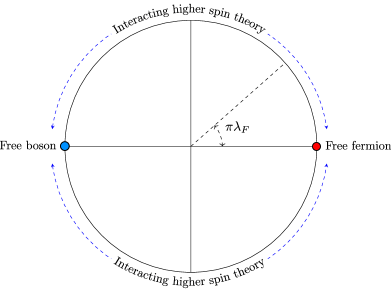
Figure 1: A chart visualizing the space of theories. Exactly conserved or weakly broken at large$-N$ higher spin theories lie on the circle of unit radius.

The above figure summarises our finding that correlation functions in CS matter theory are obtainable from the free theories with some anyonic phase factor Jain:2021whr . For two and three point functions we can just start with the FB or FF answer and appropriately multiply with the anyonic phase factor to obtain the result in CS matter theory. For the four and higher point we do require both the FF and the FB results to get the result for the CS matter theory.

4 Mapping Slightly broken HS correlators to free theory correlators

In the previous section we saw that the results in the QF theory can be written in terms of the FF and FB theory results. In this section we outline the methodology which maps correlation functions in SBHS theories to the free theories. In the next section we show how our methodology works explicitly.

4.1 Method

We make use of the SBHS equation following Maldacena:2012sf to compute the result for correlation functions. Our method can be summarised by the following flowchart.

Figure 2: Flowchart

Step 1: Choose an appropriate charge operator and a seed correlator to write down the higher spin equation in the interacting theory, say the quasi fermionic theory.

Step 2: Repeat the same for the free and critical theories.

Step 3: Write down the ansatz for each correlator that appears in the slightly broken higher spin equation in the interacting theory.

Step 4: Map the equations that are at the lowest $O(\tilde{\lambda}^{0})$ and highest orders in the coupling to the free fermion and critical bosonic theories respectively. This helps us identify the contributions at the lowest and highest orders as the ones from the free and critical theories, respectively.

Step 5: Write the pole equations which are obtained by expanding the HSE around $\tilde{\lambda}=\pm i$ to obtain the remaining unknowns in the ansatz .

Step 6: Plug back the solution in the higher spin equation and map it to a linear combination of the equations in the free and critical theories .
The above map allows us to identify the unknowns in the ansatz of the interacting theory correlator purely in terms of the FF and CB theory results.

5 Example: 3 point functions

The aim of this section is to implement the methodology described in the flowchart 2. The case of two-point functions is straightforward and is dealt with in the appendix E. We illustrate our methodology for three point functions. The simplest spinning correlator is of the kind $\langle J_{s}OO\rangle$. However, we know from (3.2) that this correlator does not have an odd contribution and is completely fixed by the free theory correlator. We start with the simplest nontrivial correlator $\langle JJO\rangle.$

5.1 $\langle JJO\rangle_{\text{QF}}$

As discussed earlier in (3.2), $\langle J_{\alpha}J_{\beta}O\rangle$ in the QF theory has an odd part. In our analysis we make use of higher spin equations and follow the steps given in the flowchart 2.

Step 1: We choose the charge operator and the seed correlator to be $Q_{3}$ and $\langle JOO\rangle$ respectively to write the following HSE in position space Jain:2020puw

$$\langle[Q_{\mu\nu},J_{\alpha}(x_{1})]O(x_{2})O(x_{3})\rangle_{\text{QF}}+\langle J_{\alpha}(x_{1})[Q_{\mu\nu},O(x_{2})]O(x_{3})\rangle_{\text{QF}}$$ (48)

$$+\langle J_{\alpha}(x_{1})O(x_{2})[Q_{\mu\nu},O(x_{3})]\rangle_{\text{QF}}=\int_{x}\langle\partial_{\sigma}J^{\sigma}_{\mu\nu}(x)J_{\alpha}(x_{1})O(x_{2})O(x_{3})\rangle_{\text{QF}}.$$ (49)

We utilize the higher spin algebra (277) and the current non conservation for $J_{\mu\nu\rho}$ (264) in the HSE (48). We then perform an integration by parts and use the large $N$ factorisation of the 5-point correlator that appears on the RHS. After a subsequent Fourier transform of the HSE we obtain the following HSE as an algebraic equation in terms of the correlators of the interacting theory

$$p_{1(\mu}\langle T_{\nu)\alpha}(p_{1})O(p_{2})O(p_{3})\rangle_{\text{QF}}+p_{1\alpha}\langle T_{\mu\nu}(p_{1})O(p_{2})O(p_{3})\rangle_{\text{QF}}$$ (50)

$$+\bigg{(}\epsilon_{(\mu ab}p_{2a}p_{2\nu)}\langle J_{\alpha}(p_{1})J_{b}(p_{2})O(p_{3})\rangle_{\text{QF}}+\left\{2\leftrightarrow 3\right\}\bigg{)}$$

$$=\bigg{(}\frac{1\tilde{\lambda}}{1+\tilde{\lambda}^{2}}p_{2(\mu}p_{2}\langle J_{\alpha}(p_{1})J_{\nu)}(p_{2})O(p_{3})\rangle_{\text{QF}}+\left\{2\leftrightarrow 3\right\}\bigg{)}$$

where the notation $p_{1(\mu}T_{\nu)\alpha}$ denotes $\mu,\nu$ symmetrisation of $p_{1\mu}T_{\nu\alpha}$. We note that Fourier transforming $\eqref{jjohse}$ gets rid of the integral on the RHS of (48) and thus makes it easier to factorise the resulting 5-point function Jain:2020puw .

Step 2: We now write down the corresponding HSEs for the FF theory

$$p_{1(\mu}\langle T_{\nu)\alpha}(p_{1})O(p_{2})O(p_{3})\rangle_{\text{FF}}+p_{1\alpha}\langle T_{\mu\nu}(p_{1})O(p_{2})O(p_{3})\rangle_{\text{FF}}$$ (51)

$$+\bigg{(}\epsilon_{(\mu ab}p_{2a}p_{2\nu)}\langle J_{\alpha}(p_{1})J_{b}(p_{2})O(p_{3})\rangle_{\text{FF}}+\left\{2\leftrightarrow 3\right\}\bigg{)}=0$$

and the CB theory,

$$p_{1(\mu}\langle T_{\nu)\alpha}(p_{1})O(p_{2})O(p_{3})\rangle_{\text{CB}}+c_{2}p_{1\alpha}\langle T_{\mu\nu}(p_{1})O(p_{2})O(p_{3})\rangle_{\text{CB}}$$ (52)

$$=p_{2(\mu}p_{2}\langle J_{\alpha}(p_{1})J_{\nu)}(p_{2})O(p_{3})\rangle_{\text{CB}}+\left\{2\leftrightarrow 3\right\}$$ (53)

Step 3: We consider the following ansatz for the correlators that appear in the HSE (50) Maldacena:2012sf

$$\begin{split}\langle T_{\nu\alpha}(p_{1})O(p_{2})O(p_{3})\rangle_{\text{QF}}&=\tilde{N}(1+\tilde{\lambda}^{2})\langle T_{\nu\alpha}(p_{1})O(p_{2})O(p_{3})\rangle_{\text{FF}}\\ \langle J_{\alpha}(p_{1})J_{\beta}(p_{2})O(p_{3})\rangle_{\text{QF}}&=\tilde{N}\langle J_{\alpha}(p_{1})J_{\beta}(p_{2})O(p_{3})\rangle_{Y_{0}}+\tilde{N}\tilde{\lambda}\langle J_{\alpha}(p_{1})J_{\beta}(p_{2})O(p_{3})\rangle_{\text{odd}}\end{split}$$ (54)

where $\langle J_{\alpha}(p_{1})J_{\beta}(p_{2})O(p_{3})\rangle_{Y_{0}}$ and $\langle J_{\alpha}(p_{1})J_{\beta}(p_{2})O(p_{3})\rangle_{\text{odd}}$ are the unknown parts that we wish to find. The HSE (50) can then be written at different orders in the coupling.

Step 4: At $O(\tilde{\lambda}^{0})$ of (50) the HSE is identical to the FF theory equation (51) which gives

$$\langle J_{\alpha}(p_{1})J_{\beta}(p_{2})O(p_{3})\rangle_{Y_{0}}=\langle J_{\alpha}(p_{1})J_{\beta}(p_{2})O(p_{3})\rangle_{FF}.$$ (55)

Similarly, the highest order equation, namely the one at $O(\tilde{\lambda}^{2})$ is identical to the CB equation (52). Thus, we identify

$$\langle J_{\alpha}(p_{1})J_{\beta}(p_{2})O(p_{3})\rangle_{\text{odd}}=\langle J_{\alpha}(p_{1})J_{\beta}(p_{2})O(p_{3})\rangle_{\text{CB}}$$ (56)

$$\langle T_{\nu\alpha}(p_{1})O(p_{2})O(p_{3})\rangle_{\text{FF}}=\langle T_{\nu\alpha}(p_{1})O(p_{2})O(p_{3})\rangle_{\text{CB}}$$ (57)

Step 5:We now write the pole equation. We expand (50) around the pole $\tilde{\lambda}=\pm i$ to get the following pole equations

$$\epsilon_{(\mu ab}p_{2a}p_{2\nu)}\langle J_{\alpha}(p_{1})J_{b}(p_{2})O(p_{3})\rangle_{\text{odd}}+\left\{2\leftrightarrow 3\right\}=p_{2(\mu}p_{2}\langle J_{\alpha}(p_{1})J_{\nu)}(p_{2})O(p_{3})\rangle_{\text{FF}}+\left\{2\leftrightarrow 3\right\}$$ (58)

$$\epsilon_{(\mu ab}p_{2a}p_{2\nu)}\langle J_{\alpha}(p_{1})J_{b}(p_{2})O(p_{3})\rangle_{\text{FF}}+\left\{2\leftrightarrow 3\right\}=p_{2(\mu}p_{2}\langle J_{\alpha}(p_{1})J_{\nu)}(p_{2})O(p_{3})\rangle_{\text{odd}}+\left\{2\leftrightarrow 3\right\}$$ (59)

which helps us identify the unknown correlator $\langle J_{\alpha}(p_{1})J_{\nu}(p_{2})O(p_{3})\rangle_{\text{odd}}$ in terms of the same correlator in free theory Jain:2021gwa ; Gandhi:2021gwn

$$\langle J_{\alpha}(p_{1})J_{\nu}(p_{2})O(p_{3})\rangle_{\text{odd}}=\frac{1}{p_{2}}\epsilon_{\nu ab}\,p_{2a}\,\langle J_{\alpha}(p_{1})J_{b}(p_{2})O(p_{3})\rangle_{\text{FF}}$$ (60)

The expression for $\langle JJO\rangle_{\text{odd}}$ obtained from (60) is consistent with the results obtained using perturbative techniques in special kinematic regimes Aharony:2012nh ; GurAri:2012is and by solving conformal Ward identities in momentum space Jain:2021gwa ; Gandhi:2021gwn .

Step 6: We now use our results to map the SBHS equation to the free theory HSE. To do this, we use (60) and substitute it back into (50) and see that the remaining HSE maps to the free theory equation. Thus we see that the solution for the odd piece that we obtained from the pole equation is consistent with the HSE at any order.

This confirms the result obtained for $\langle J_{\alpha}(p_{1})J_{\beta}(p_{2})O(p_{3})\rangle_{\text{odd}}$ in (58). Thus we have completely determined the 3-point spinning correlator $\langle J_{\alpha}(p_{1})J_{\beta}(p_{2})O(p_{3})\rangle_{\text{odd}}$ in the interacting theory purely in terms of free theory correlators i.e

$$\langle J_{\alpha}(p_{1})J_{\beta}(p_{2})O(p_{3})\rangle_{\text{QF}} =\tilde{N}\langle J_{\alpha}(p_{1})J_{\beta}(p_{2})O(p_{3})\rangle_{\text{FF}}+\tilde{N}\tilde{\lambda}\frac{\epsilon_{\beta ab}\,p_{2a}}{p_{2}}\langle J_{\alpha}(p_{1})J_{b}(p_{2})O(p_{3})\rangle_{\text{FF}}$$ (61)

Now in spinor-helicity we have $\langle\epsilon\cdot JJO\rangle\rightarrow\pm i\langle JJO\rangle$ depending on the helicity. Thus the final expression becomes,

$$\langle JJO\rangle_{\text{QF}} =\tilde{N}(1+i\tilde{\lambda})\langle JJO\rangle_{\text{FF}}$$ (62)

$$=\frac{iN(1-e^{-i\pi\lambda_{f}})}{\pi\lambda_{f}}\langle JJO\rangle_{\text{FF}}$$ (63)

We note that the expression of the correlator picks up an anyonic phase when we express the full correlator only in terms of the FF theory correlator.

5.2 $\langle TTO\rangle_{\text{QF}}$

We now compute the correlator $\langle T_{\alpha\beta}T_{\mu\nu}O\rangle$ in the QF theory. The analysis here is very similar to $\langle JJO\rangle_{\text{QF}}$ obtained in the previous section. We make use of the higher spin algebra of $Q_{4}$ in (277) and (280) and the current non-conservation equation associated to $J_{4}$ in (264) to obtain the momentum space HSE in terms of the interacting theory correlators.

Now we assume $\langle TTO\rangle_{\text{QF}}$ has the following structure

$$\langle T_{\alpha\beta}(p_{1})T_{\gamma\delta}(p_{2})O(p_{3})\rangle_{\text{QF}}=\tilde{N}\langle T_{\alpha\beta}(p_{1})T_{\gamma\delta}(p_{2})O(p_{3})\rangle_{Y_{0}}+\tilde{N}\tilde{\lambda}\langle T_{\alpha\beta}(p_{1})T_{\gamma\delta}(p_{2})O(p_{3})\rangle_{\text{odd}}$$ (64)

Repeating the steps as in the previous section, we obtain a set of algebraic equations at different orders in the coupling. The $O(\tilde{\lambda}^{0})$ equation is the free theory equation after we identify

$$\langle T_{\alpha\beta}(p_{1})T_{\gamma\delta}(p_{2})O(p_{3})\rangle_{Y_{0}} =\langle T_{\alpha\beta}(p_{1})T_{\gamma\delta}(p_{2})O(p_{3})\rangle_{\text{FF}}$$ (65)

The pole equations help us identify $\langle TTO\rangle_{\text{odd}}$ in terms of the same correlator in the free theory

$$\langle T_{\alpha\beta}(p_{1})T_{\gamma\delta}(p_{2})O(p_{3})\rangle_{\text{odd}} =\epsilon_{\gamma ab}\frac{p_{2a}}{p_{2}}\langle T_{\alpha\beta}(p_{1})T_{b\delta}(p_{2})O(p_{3})\rangle_{\text{FF}}$$ (66)

We then substitute this back (65), (66) in the SBHS equation and map it to the free theory equation. Therefore the interacting theory correlator $\langle TTT\rangle_{\text{QF}}$ is given by

$$\langle T_{\alpha\beta}(p_{1})T_{\gamma\delta}(p_{2})O(p_{3})\rangle_{\text{QF}} =\tilde{N}\langle T_{\alpha\beta}(p_{1})T_{\gamma\delta}(p_{2})O(p_{3})\rangle_{\text{FF}}+\tilde{N}\tilde{\lambda}\epsilon_{\gamma ab}\frac{p_{2a}}{p_{2}}\langle T_{\alpha\beta}(p_{1})T_{b\delta}(p_{2})O(p_{3})\rangle_{\text{FF}}$$ (67)

Now in spinor-helicity we have $\langle\epsilon\cdot TTO\rangle\rightarrow\pm i\langle TTO\rangle$. Thus the final expression becomes,

$$\langle TTO\rangle_{\text{QF}} =\tilde{N}(1+i\tilde{\lambda})\langle TTO\rangle_{\text{FF}}$$ (68)

$$=\frac{iN(1-e^{-i\pi\lambda_{f}})}{\pi\lambda_{f}}\langle TTO\rangle_{\text{FF}}$$ (69)

Yet again we see that the expression of the correlator picks up an anyonic phase.

5.3 $\langle TTT\rangle_{\text{QF}}$

In this section we will make use of the HSE to obtain the odd part of $\langle TTT\rangle$ in the QF theory. As before we follow the algorithm shown in the flowchart.

Step 1: We choose the charge operator and the seed correlator to be $Q_{4}$ and $\langle OTT\rangle$ respectively to write the following HSE in position space

$$\langle[Q_{\mu\nu\rho},O(x_{1})]T_{\alpha\beta}(x_{2})T_{\gamma\theta}(x_{3})\rangle_{\text{QF}}+\langle O(x_{1})[Q_{\mu\nu\rho},T_{\alpha\beta}(x_{2})]T_{\gamma\theta}(x_{3})]\rangle_{\text{QF}}$$ (70)

$$+\langle O(x_{1})T_{\alpha\beta}(x_{2})[Q_{\mu\nu\rho},T_{\gamma\theta}(x_{3})]\rangle_{\text{QF}}=\int_{x}\langle\partial_{\sigma}J^{\sigma}_{\mu\nu\rho}(x)O(x_{1})T_{\alpha\beta}(x_{2})T_{\gamma\theta}(x_{3})\rangle_{\text{QF}}$$ (71)

We make use of the higher spin algebra (277) and (280) along with the current non conservation (264) to obtain the following HSE in momentum space

$$p_{1(\mu}p_{1\nu}p_{1\rho)}\langle O(p_{1})T_{\alpha\beta}(p_{2})T_{\gamma\theta}(p_{3})\rangle_{\text{QF}}+\epsilon_{(\mu ab}p_{1a}p_{1\nu}\langle T_{b\rho)}(p_{1})T_{\alpha\beta}(p_{2})T_{\gamma\theta}(p_{3})\rangle_{\text{QF}}$$ (72)

$$+\bigg{(}p_{2(\mu}p_{2\nu}p_{2\rho)}\langle O(p_{1})T_{\alpha\beta}(p_{2})T_{\gamma\theta}(p_{3})\rangle_{\text{QF}}$$ (73)

$$\hskip 28.45274pt+p_{2(\mu}p_{2\nu}p_{2\alpha}\langle O(p_{1})T_{\rho)\beta}(p_{2})T_{\gamma\theta}(p_{3})\rangle_{\text{QF}}+\left\{2\leftrightarrow 3\right\}\bigg{)}=$$ (74)

$$\frac{\tilde{\lambda}}{1+\tilde{\lambda}^{2}}\Bigg{[}{p_{1(\mu}}p_{1}\langle T_{\nu\rho)}(p_{2})T_{\alpha\beta}(p_{2})T_{\gamma\theta}(p_{3})\rangle_{\text{QF}}+\bigg{(}p_{2(\mu}\langle T_{\nu\rho)}T_{\alpha\beta}\rangle_{\text{QF}}\langle O(p_{1})O(p_{2})T_{\gamma\theta}(p_{3})\rangle_{\text{QF}}$$ (75)

$$+\left\{2\leftrightarrow 3\right\}\bigg{)}\Bigg{]}$$ (76)

Step 2: We now write down the corresponding higher spin equation for the FF theory

$$p_{1(\mu}p_{1\nu}p_{1\rho)}\langle O(p_{1})T_{\alpha\beta}(p_{2})T_{\gamma\theta}(p_{3})\rangle_{\text{FF}}-\epsilon_{(\mu ab}p_{1a}p_{1\nu}\langle T_{b\rho)}(p_{1})T_{\alpha\beta}(p_{2})T_{\gamma\theta}(p_{3})\rangle_{\text{FF}}$$ (77)

$$+\left(p_{2(\mu}p_{2\nu}p_{2\rho)}\langle O(p_{1})T_{\alpha\beta}(p_{2})T_{\gamma\theta}(p_{3})\rangle_{\text{FF}}\right.$$ (78)

$$\left.\hskip 28.45274pt+p_{2(\mu}p_{2\nu}p_{2\alpha}\langle O(p_{1})T_{\rho)\beta}(p_{2})T_{\gamma\theta}(p_{3})\rangle_{\text{FF}}+\left\{2\leftrightarrow 3\right\}\right)=0$$ (79)

and similarly for the CB theory,

$$p_{1(\mu}p_{1\nu}p_{1\rho)}\langle O(p_{1})T_{\alpha\beta}(p_{2})T_{\gamma\theta}(p_{3})\rangle_{\text{CB}}+\left(p_{2(\mu}p_{2\nu}p_{2\rho)}\langle O(p_{1})T_{\alpha\beta}(p_{2})T_{\gamma\theta}(p_{3})\rangle_{\text{CB}}\right.$$ (80)

$$\left.\hskip 113.81102pt+p_{2(\mu}p_{2\nu}p_{2\alpha}\langle O(p_{1})T_{\rho)\beta}(p_{2})T_{\gamma\theta}(p_{3})\rangle_{\text{CB}}+\left\{2\leftrightarrow 3\right\}\right)$$ (81)

$$=\bigg{[}p_{1(\mu}p_{1}\langle T_{\nu\rho)}(p_{1})T_{\alpha\beta}(p_{2})T_{\gamma\theta}(p_{3})\rangle_{\text{CB}}+\bigg{(}p_{2(\mu}\langle T_{\nu\rho)}T_{\alpha\beta}\rangle_{\text{QF}}\langle O(p_{1})O(p_{2})T_{\gamma\theta}(p_{3})\rangle_{\text{CB}}$$ (82)

$$+\left\{2\leftrightarrow 3\right\}\bigg{)}\Bigg{]}$$ (83)

Step 3: We consider the following ansatz for the correlators that appear in the HSE (72) Maldacena:2012sf

$$\begin{split}\langle O(p_{1})O(-p_{1})\rangle_{\text{QF}}&=\tilde{N}(1+\tilde{\lambda}^{2})\langle O(p_{1})O(-p_{1})\rangle_{\text{FF}}\\ \langle O(p_{1})T_{\alpha\beta}(p_{2})T_{\gamma\theta}(p_{3})\rangle_{\text{QF}}&=\tilde{N}\langle O(p_{1})T_{\alpha\beta}(p_{2})T_{\gamma\theta}(p_{3})\rangle_{\text{FF}}+\tilde{N}\tilde{\lambda}\langle O(p_{1})T_{\alpha\beta}(p_{2})T_{\gamma\theta}(p_{3})\rangle_{\text{CB}}\\ \langle T_{\rho\sigma}(p_{1})T_{\alpha\beta}(p_{2})T_{\gamma\theta}(p_{3})\rangle_{\text{QF}}&=\tilde{N}\frac{1}{1+\tilde{\lambda}^{2}}\left[\langle T_{\rho\sigma}(p_{1})T_{\alpha\beta}(p_{2})T_{\gamma\theta}(p_{3})\rangle_{Y_{0}}\right.\cr&\left.+\tilde{\lambda}^{2}\langle T_{\rho\sigma}(p_{1})T_{\alpha\beta}(p_{2})T_{\gamma\theta}(p_{3})\rangle_{Y_{2}}+\tilde{\lambda}\langle T_{\rho\sigma}(p_{1})T_{\alpha\beta}(p_{2})T_{\gamma\theta}(p_{3})\rangle_{odd}\right]\end{split}$$ (84)

Our goal is to determine the parity odd part of $\langle TTT\rangle$, viz. $\langle T_{\rho\sigma}(p_{1})T_{\alpha\beta}(p_{2})T_{\gamma\theta}(p_{3})\rangle_{\text{odd}}$ in terms of the free theory correlators. We can now write the HSE at various orders in the coupling constant.

Step 4: At $O(\tilde{\lambda}^{0})$ of (72), the HSE is identical to the FF HSE (77) which gives

$$\langle T_{\rho\sigma}(p_{1})T_{\alpha\beta}(p_{2})T_{\gamma\theta}(p_{3})\rangle_{Y_{0}}=\langle T_{\rho\sigma}(p_{1})T_{\alpha\beta}(p_{2})T_{\gamma\theta}(p_{3})\rangle_{\text{FF}}$$ (85)

Similarly, the highest order equation namely the $O(\tilde{\lambda}^{3})$ is identical to the critical bosonic equation (80) since the CB theory is the $\tilde{\lambda}\rightarrow\infty$ limit of the QF theory. This happens after we identify

$$\langle T_{\rho\sigma}(p_{1})T_{\alpha\beta}(p_{2})T_{\gamma\theta}(p_{3})\rangle_{Y_{2}}=\langle T_{\rho\sigma}(p_{1})T_{\alpha\beta}(p_{2})T_{\gamma\theta}(p_{3})\rangle_{\text{CB}}$$ (86)

Hence we get 2 of the 3 unknowns.

Step 5: To find the third unknown we expand (72) around the pole $\tilde{\lambda}=\pm i$ to get the following pole equations

$$\epsilon_{(\mu ab}p_{1a}p_{1\nu}\langle T_{b\rho)}(p_{1})T_{\alpha\beta}(p_{2})T_{\gamma\theta}(p_{3})\rangle_{\text{odd}}$$ (87)

$$=p_{1(\mu}p_{1}\bigg{(}\langle T_{\nu\rho)}(p_{1})T_{\alpha\beta}(p_{2})T_{\gamma\theta}(p_{3})\rangle_{\text{FB}}-\langle T_{\nu\rho}(p_{1})T_{\alpha\beta}(p_{2})T_{\gamma\theta}(p_{3})\rangle_{\text{FF}}\bigg{)}$$ (88)

$$\epsilon_{(\mu ab}p_{1a}p_{1\nu}\bigg{(}\langle T_{b\rho)}(p_{1})T_{\alpha\beta}(p_{2})T_{\gamma\theta}(p_{3})\rangle_{\text{FB}}-\langle T_{b\rho)}(p_{1})T_{\alpha\beta}(p_{2})T_{\gamma\theta}(p_{3})\rangle_{\text{FF}}\bigg{)}$$ (89)

$$=p_{1(\mu}p_{1}\langle T_{\nu\rho)}(p_{1})T_{\alpha\beta}(p_{2})T_{\gamma\theta}(p_{3})\rangle_{\text{odd}}$$ (90)

which helps us identify the unknown correlator $\langle T_{\nu\rho}(p_{1})T_{\alpha\beta}(p_{2})T_{\gamma\theta}(p_{3})\rangle_{\text{odd}}$ in terms of the same correlator in the free theories. Thus from (84), after contracting with $\Pi_{\mu\nu}(p_{1})$ and $p_{1\rho}$ we get $\langle TTT\rangle_{\text{odd}}$ to be

$$\langle T_{\mu\nu}(p_{1})T_{\alpha\beta}(p_{2})T_{\gamma\theta}(p_{3})\rangle_{\text{odd}}$$ (91)

$$=\frac{1}{p_{1}}\epsilon_{\mu ab}p_{1a}\bigg{(}\langle T_{b\nu}(p_{1})T_{\alpha\beta}(p_{2})T_{\gamma\theta}(p_{3})\rangle_{\text{FB}}-\langle T_{b\rho)}(p_{1})T_{\alpha\beta}(p_{2})T_{\gamma\theta}(p_{3})\rangle_{\text{FF}}\bigg{)}$$ (92)

Step 6: We now use our results to map the SBHS equation to the free theory HSE. We use the expression for $\langle TTT\rangle_{\text{odd}}$ and substitute it back into the $O(\tilde{\lambda})$ and $O(\tilde{\lambda}^{2})$ equations and see that they map to the free theory equations. Therefore we see that that our solution for $\langle TTT\rangle_{\text{odd}}$ obtained from (91) solves the entire higher spin equation and is also consistent with results obtained in Jain:2021gwa ; Gandhi:2021gwn . The same can also be obtained by solving conformal Ward identities in momentum space. Thus we have seen that in the QF theory the correlator $\langle TTT\rangle$ is given by

$$\langle TTT\rangle_{\text{QF}} =\frac{\tilde{N}}{1+\tilde{\lambda}^{2}}\big{(}\langle TTT\rangle_{\text{FF}}+\tilde{\lambda}\langle TTT\rangle_{\text{odd}}+\tilde{\lambda}^{2}\langle TTT\rangle_{\text{FB}}\big{)}$$ (93)

$$=\frac{\tilde{N}}{2}\left(\langle TTT\rangle_{\text{FF+FB}}+\frac{1-\tilde{\lambda}^{2}}{1+\tilde{\lambda}^{2}}\langle TTT\rangle_{\text{FF-FB}}+\frac{2\tilde{\lambda}}{1+\tilde{\lambda}^{2}}\langle\epsilon\cdot TTT\rangle_{\text{FB-FF}}\right)$$ (94)

Now in spinor-helicity variables we have $\langle\epsilon\cdot TTT\rangle\rightarrow i\langle TTT\rangle$ and thus

$$\langle TTT\rangle_{\text{QF}} =\frac{\tilde{N}}{2}\left(\langle TTT\rangle_{\text{FF+FB}}+\left(\frac{1+i\tilde{\lambda}}{1-i\tilde{\lambda}}\right)\langle TTT\rangle_{\text{FF-FB}}\right)$$ (95)

$$=\frac{\tilde{N}}{2}\left(\langle TTT\rangle_{\text{FF+FB}}+e^{-i\pi\lambda_{f}}\langle TTT\rangle_{\text{FF-FB}}\right)$$ (96)

Thus we see the presence of an anyonic phase yet again in the expression for the correlator. There is one more representation which makes the duality manifest

$$\langle TTT\rangle_{\text{QF}} =e^{-i\pi\frac{\lambda_{f}}{2}}\left(\cos\frac{\pi\lambda_{f}}{2}\langle TTT\rangle_{\text{FF}}+i\sin\frac{\pi\lambda_{f}}{2}\langle TTT\rangle_{\text{FB}}\right)$$ (97)

Note that at $\lambda_{f}=0$ it gives the FF and at $\lambda_{f}=1,$ it gives the FB answer.

5.4 $\langle J_{s_{1}}J_{s_{2}}T\rangle_{QF}$

In this section we use HSEs to constrain the general 3-point correlator $\langle J_{s_{1}}J_{s_{2}}T\rangle$ in the QF theory. We choose the charge operator and the seed correlator to be $Q_{4}$ and $\langle J_{s_{1}}J_{s_{2}}O\rangle$ respectively. The relevant operator algebra is given by Maldacena:2012sf

$$[Q_{4},J_{s}] =c_{s,s-2}\partial^{5}J_{s-2}+c_{s,s}\partial^{3}J_{s}+c_{s,s+2}\partial J_{s+2}$$ (98)

$$[Q_{4},O] =\partial^{3}O+\epsilon\cdot\partial T$$ (99)

To solve the resulting HSEs we make use of the following structure of the correlators,

$$\langle OO\rangle_{\text{QF}} =\tilde{N}(1+\tilde{\lambda}^{2})\langle OO\rangle_{\text{FF}}$$ (100)

$$\langle J_{s_{1}}J_{s_{2}}O\rangle_{\text{QF}} =\tilde{N}\langle J_{s_{1}}J_{s_{2}}O\rangle_{\text{FF}}+\tilde{N}\tilde{\lambda}\langle J_{s_{1}}J_{s_{2}}O\rangle_{\text{odd}}$$ (101)

$$\langle J_{s_{1}}J_{s_{2}}T\rangle_{\text{QF}} =\tilde{N}\frac{1}{1+\tilde{\lambda}^{2}}\big{(}\langle J_{s_{1}}J_{s_{2}}T\rangle_{Y_{0}}+\tilde{\lambda}\langle J_{s_{1}}J_{s_{2}}T\rangle_{\text{odd}}+\tilde{\lambda}^{2}\langle J_{s_{1}}J_{s_{2}}T\rangle_{Y_{2}}\big{)}$$ (102)

where our goal is to obtain $\langle J_{s_{1}}J_{s_{2}}T\rangle_{Y_{0}}$, $\langle J_{s_{1}}J_{s_{2}}T\rangle_{Y_{2}}$ ,$\langle J_{s_{1}}J_{s_{2}}T\rangle_{\text{odd}}$ in terms of the free theory correlators. We use the free and critical theory equations to identify two unknowns

$$\langle J_{s_{1}}J_{s_{2}}T\rangle_{Y_{0}}=\langle J_{s_{1}}J_{s_{2}}T\rangle_{\text{FF}}$$ (103)

$$\langle J_{s_{1}}J_{s_{2}}T\rangle_{Y_{2}}=\langle J_{s_{1}}J_{s_{2}}T\rangle_{\text{CB}}$$ (104)

The pole equations take the form

$$\langle J_{s_{1}}J_{s_{2}}T\rangle_{\text{FF}}-\langle J_{s_{1}}J_{s_{2}}T\rangle_{\text{CB}}=\epsilon\cdot\langle J_{s_{1}}J_{s_{2}}T\rangle_{\text{odd}}$$ (105)

$$\langle J_{s_{1}}J_{s_{2}}T\rangle_{\text{odd}}=\epsilon\cdot\bigg{(}\langle J_{s_{1}}J_{s_{2}}T\rangle_{\text{FF}}-\langle J_{s_{1}}J_{s_{2}}T\rangle_{\text{CB}}\bigg{)}$$ (106)

where the dot indicates a contraction of the Levi-Civita tensor with one of the indices of the spin $s_{1}$ current in the correlator. From the second equation in (105) we obtain the remaining unknown piece of $\langle J_{s_{1}}J_{s_{2}}T\rangle_{\text{QF}}$

$$\langle J_{s_{1}}J_{s_{2}}T\rangle_{\text{odd}}=\epsilon\cdot\bigg{(}\langle J_{s_{1}}J_{s_{2}}T\rangle_{\text{FF}}-\langle J_{s_{1}}J_{s_{2}}T\rangle_{\text{CB}}\bigg{)}$$ (107)

Therefore we have the full correlator in the QF theory given by

$$\langle J_{s_{1}}J_{s_{2}}T\rangle_{\text{QF}}=\tilde{N}\frac{1}{1+\tilde{\lambda}^{2}}\left(\langle J_{s_{1}}J_{s_{2}}T\rangle_{FF}+\tilde{\lambda}\epsilon\cdot\left(\langle J_{s_{1}}J_{s_{2}}T\rangle_{\text{FF}}-\langle J_{s_{1}}J_{s_{2}}T\rangle_{\text{CB}}\right)+\tilde{\lambda}^{2}\langle J_{s_{1}}J_{s_{2}}T\rangle_{CB}\right)$$ (108)

It can be easily checked that the higher spin equations at all orders are satisfied by the above expression for $\langle J_{s_{1}}J_{s_{2}}T\rangle_{\text{odd}}$.

5.5 $\langle J_{s_{1}}J_{s_{2}}J_{s_{3}}\rangle_{QF}$

In this section we use HSEs to constrain the general 3-point correlator $\langle J_{s_{1}}J_{s_{2}}J_{s_{3}}\rangle$ with $s_{i}>2$ in the QF theory. We look at the Ward identity corresponding to the non-conservation equation of the spin-4 current in the correlator $\langle J_{s_{1}}J_{s_{2}}J_{s_{3}}\rangle_{\text{QF}}$. We use the relevant operator algebra (98) for $J_{s}$. The current non-conservation does not contribute to the RHS after we perform a large $N$ factorisation of the resulting 5-point function. The momentum space HSE becomes

$$c_{s_{1},s_{1}-2}p_{1\mu}p_{1\nu}p_{1\rho}p_{1\alpha_{1}}p_{1\alpha_{2}}\langle J_{\alpha_{3}\alpha_{4}...\alpha_{s_{1}}}J_{\beta_{1}\beta_{2}...\beta_{s_{2}}}J_{\gamma_{1}\gamma_{2}...\gamma_{s_{3}}}\rangle_{QF}$$ (109)

$$+c_{s_{1},s_{1}}p_{1\mu}p_{1\nu}p_{1\rho}\langle J_{\alpha_{1}\alpha_{2}...\alpha_{s_{1}}}J_{\beta_{1}\beta_{2}...\beta_{s_{2}}}J_{\gamma_{1}\gamma_{2}...\gamma_{s_{3}}}\rangle_{QF}$$ (110)

$$+c_{s_{1},s_{1}+2}p_{1\mu}\langle J_{\nu\rho\alpha_{1}\alpha_{2}...\alpha_{s_{1}}}J_{\beta_{1}\beta_{2}...\beta_{s_{2}}}J_{\gamma_{1}\gamma_{2}...\gamma_{s_{3}}}\rangle_{QF}+\{1\leftrightarrow 2\}+\{1\leftrightarrow 3\}=0$$ (111)

The corresponding FF equation is

$$c_{s_{1},s_{1}-2}p_{1\mu}p_{1\nu}p_{1\rho}p_{1\alpha_{1}}p_{1\alpha_{2}}\langle J_{\alpha_{3}\alpha_{4}...\alpha_{s_{1}}}J_{\beta_{1}\beta_{2}...\beta_{s_{2}}}J_{\gamma_{1}\gamma_{2}...\gamma_{s_{3}}}\rangle_{FF}$$ (112)

$$+c_{s_{1},s_{1}}p_{1\mu}p_{1\nu}p_{1\rho}\langle J_{\alpha_{1}\alpha_{2}...\alpha_{s_{1}}}J_{\beta_{1}\beta_{2}...\beta_{s_{2}}}J_{\gamma_{1}\gamma_{2}...\gamma_{s_{3}}}\rangle_{FF}$$ (113)

$$+c_{s_{1},s_{1}+2}p_{1\mu}\langle J_{\nu\rho\alpha_{1}\alpha_{2}...\alpha_{s_{1}}}J_{\beta_{1}\beta_{2}...\beta_{s_{2}}}J_{\gamma_{1}\gamma_{2}...\gamma_{s_{3}}}\rangle_{FF}+\{1\leftrightarrow 2\}+\{1\leftrightarrow 3\}=0$$ (114)

We use the following ansatz for the general 3-point spinning correlator

$$\langle J_{s_{1}}J_{s_{2}}J_{s_{3}}\rangle_{QF}=\frac{\tilde{N}}{1+\tilde{{\lambda}}^{2}}\bigg{(}\langle J_{s_{1}}J_{s_{2}}J_{s_{3}}\rangle_{Y_{0}}+\tilde{\lambda}\langle J_{s_{1}}J_{s_{2}}J_{s_{3}}\rangle_{\text{odd}}+\tilde{\lambda}^{2}\langle J_{s_{1}}J_{s_{2}}J_{s_{3}}\rangle_{Y_{2}}\bigg{)}$$ (115)

where $\langle J_{s_{1}}J_{s_{2}}J_{s_{3}}\rangle_{Y_{0}}$, $\langle J_{s_{1}}J_{s_{2}}J_{s_{3}}\rangle_{\text{odd}}$ and $\langle J_{s_{1}}J_{s_{2}}J_{s_{3}}\rangle_{Y_{2}}$, are the unknowns that we wish to find. We substitute this back into (109) and see that the $O(\tilde{\lambda}^{0})$ equation is like the FF equation after we identify

$$\langle J_{\alpha_{3}\alpha_{4}...\alpha_{s_{1}}}J_{\beta_{1}\beta_{2}...\beta_{s_{3}}}J_{\gamma_{1}\gamma_{2}...\gamma_{s_{3}}}\rangle_{Y_{0}}=J_{\alpha_{3}\alpha_{4}...\alpha_{s_{1}}}J_{\beta_{1}\beta_{2}...\beta_{s_{3}}}J_{\gamma_{1}\gamma_{2}...\gamma_{s_{3}}}\rangle_{FF}$$ (116)

The highest order equation in $\tilde{\lambda}$ in (109) is like the CB equation. This can be seen after we use the CB algebra to write the CB higher spin equation and identify

$$\langle J_{\nu\rho\alpha_{1}\alpha_{2}...\alpha_{s_{1}}}J_{\beta_{1}\beta_{2}...\beta_{s_{3}}}J_{\gamma_{1}\gamma_{2}...\gamma_{s_{3}}}\rangle_{Y_{2}}=\langle J_{\nu\rho\alpha_{1}\alpha_{2}...\alpha_{s_{1}}}J_{\beta_{1}\beta_{2}...\beta_{s_{3}}}J_{\gamma_{1}\gamma_{2}...\gamma_{s_{3}}}\rangle_{CB}$$ (117)

We now use the following ansatz for $\langle J_{s_{1}}J_{s_{2}}J_{s_{3}}\rangle_{\text{odd}}$

$$p_{1\mu}p_{1}\langle J_{\alpha_{1}\alpha_{2}...\alpha_{s_{1}}}J_{\beta_{1}\beta_{2}...\beta_{s_{3}}}J_{\gamma_{1}\gamma_{2}...\gamma_{s_{3}}}\rangle_{\text{odd}}=\epsilon_{\nu ab}p_{1a}p_{1\mu}\bigg{(}\langle J_{b\alpha_{2}\alpha_{3}.....\alpha_{s_{1}}}J_{\beta_{1}\beta_{2}...\beta_{s_{3}}}J_{\gamma_{1}\gamma_{2}...\gamma_{s_{3}}}\rangle_{\text{FF}}$$ (118)

$$-\langle J_{b\alpha_{2}\alpha_{3}.....\alpha_{s_{1}}}J_{\beta_{1}\beta_{2}...\beta_{s_{3}}}J_{\gamma_{1}\gamma_{2}...\gamma_{s_{3}}}\rangle_{\text{CB}}\bigg{)}$$ (119)

and plug it back into the HSE (109). The above ansatz helps map the $O(\tilde{\lambda})$ equation to the free and critical theory equations. Therefore our ansatz of $\langle J_{s_{1}}J_{s_{2}}J_{s_{3}}\rangle_{\text{odd}}$ (118) is consistent with the above set of equations. Hence we could compute $\langle J_{s_{1}}J_{s_{2}}J_{s_{3}}\rangle_{QF}$ in terms of free theory correlators as

$$\langle J_{s_{1}}J_{s_{2}}J_{s_{3}}\rangle_{QF}=\frac{\tilde{N}}{1+\tilde{\lambda}^{2}}\bigg{(}\langle J_{s_{1}}J_{s_{2}}J_{s_{3}}\rangle_{FF}+\tilde{\lambda}\epsilon\cdot\bigg{(}\langle J_{s_{1}}J_{s_{2}}J_{s_{3}}\rangle_{FF}-\langle J_{s_{1}}J_{s_{2}}J_{s_{3}}\rangle_{CB}\bigg{)}+\tilde{\lambda}^{2}\langle J_{s_{1}}J_{s_{2}}J_{s_{3}}\rangle_{CB}\bigg{)}$$ (120)

which is consistent with the result obtained by solving the conformal Ward identities in momentum space and reproduces the same result as the one obtained via perturbative calculations which are in general quite difficult.

If we now write the same in the helicity basis, the steps parallel the analysis done for $\langle TTT\rangle$ in 5.3 which gives

$$\langle J_{s_{1}}J_{s_{2}}J_{s_{3}}\rangle_{\text{QF}} =\frac{\tilde{N}}{2}\left(\langle J_{s_{1}}J_{s_{2}}J_{s_{3}}\rangle_{\text{FF+FB}}+e^{-i\pi\lambda_{f}}\langle J_{s_{1}}J_{s_{2}}J_{s_{3}}\rangle_{\text{FF-FB}}\right)$$ (121)

and thus the presence of an anyonic phase is a generic occurrence in three-point functions. Now, if the spins of the operators satisfy the triangle inequality in (16) then from the discussion in 3.2 we can write this result in terms of homogeneous/non-homogeneous parts of just the FF theory or just the FB theory.

6 Example-II: 4-point functions

In the previous section we solved for 3-point functions using HSEs. In this section we look into 4-point functions comprising of operator insertions with arbitrary spins.

6.1 $\langle TOOO\rangle_{\text{QF}}$

To start with, we look at the simple example of $\langle TOOO\rangle_{\text{QF}}.$ The result of this part was obtained first in position space by Li:2019twz , in momentum space in Jain:2020puw and in Mellin space in Silva:2021ece . Below we work in momentum space.

Step 1: We choose the charge operator and the seed correlator to be $Q_{4}$ and $\langle OOOO\rangle$ respectively. Then we make use of the higher spin algebra (277) and (280) along with the current non conservation (264) to obtain the following HSE in momentum space

$$\begin{split}&p_{1\mu}p_{1\nu}p_{1\rho}\langle OOOO\rangle_{\text{QF}}+g_{(\mu\nu}p_{1\rho)}p_{1}^{2}\langle OOOO\rangle_{\text{QF}}+\epsilon_{ab(\mu}p_{1\nu}p_{1a}\langle T_{b\rho)}OOO\rangle_{\text{QF}}\\ &+\{1\leftrightarrow 2\}+\{1\leftrightarrow 3\}+\{1\leftrightarrow 4\}=\tilde{\lambda}p_{1(\mu}p_{1}\langle T_{\nu\rho)}OOO\rangle_{\text{QF}}+\{1\leftrightarrow 2\}+\{1\leftrightarrow 3\}+\{1\leftrightarrow 4\}\end{split}$$ (122)

Step 2: We now write down the corresponding higher spin equations for the free theory

$$\begin{split}&p_{1\mu}p_{1\nu}p_{1\rho}\langle OOOO\rangle_{\text{FF}}+g_{(\mu\nu}p_{1\rho)}p_{1}^{2}\langle OOOO\rangle_{\text{FF}}+\epsilon_{ab(\mu}p_{1\nu}p_{1a}\langle T_{b\rho)}OOO\rangle_{\text{FF}}\\ &+\{1\leftrightarrow 2\}+\{1\leftrightarrow 3\}+\{1\leftrightarrow 4\}=0\end{split}$$ (123)

and similarly for the CB theory,

$$\begin{split}&p_{1(\mu}p_{1\nu}p_{1\rho)}\langle OOOO\rangle_{\text{CB}}+g_{(\mu\nu}p_{1\rho)}p_{1}^{2}\langle OOOO\rangle_{\text{CB}}+\{1\leftrightarrow 2\}+\{1\leftrightarrow 3\}+\{1\leftrightarrow 4\}\\ &=p_{1(\mu}p_{1}\langle T_{\nu\rho)}OOO\rangle_{\text{CB}}+\{1\leftrightarrow 2\}+\{1\leftrightarrow 3\}+\{1\leftrightarrow 4\}\end{split}$$ (124)

Step 3: We consider the following ansatz for the correlators that appear in the HSE (122)

$$\begin{split}&\langle TOOO\rangle_{\text{QF}}=\tilde{N}(1+\tilde{\lambda}^{2})\bigg{(}\langle TOOO\rangle_{\text{$Y_{0}$}}+\tilde{\lambda}\langle TOOO\rangle_{\text{$Y_{1}$}}\bigg{)}\cr&\langle OOOO\rangle_{\text{QF}}=\tilde{N}(1+\tilde{\lambda}^{2})(\langle OOOO\rangle_{\text{FF}}+\tilde{\lambda}^{2}\langle OOOO\rangle_{\text{CB}})\end{split}$$ (125)

Step 4: At $O(\tilde{\lambda}^{0})$ of (122) we obtain the HSE to be identical to the FF theory equation (123) which gives

$$\langle TOOO\rangle_{\text{$Y_{0}$}}=\langle TOOO\rangle_{\text{FF}}$$ (126)

Similarly, the highest order equation( $O(\tilde{\lambda}^{4})$ ) is identical to the CB equation (124) since the CB theory is the $\tilde{\lambda}\rightarrow\infty$ limit of the quasi fermionic theory. This happens after we identify

$$\langle TOOO\rangle_{\text{$Y_{1}$}}=\langle TOOO\rangle_{\text{CB}}$$ (127)

Step 5: We expand the HSE (122) around the point $\tilde{\lambda}=\pm i$ and obtain the following pole equations

$$\begin{split}&\epsilon_{ab(\mu}p_{1\nu}p_{1a}\langle T_{b\rho)}OOO\rangle_{\text{FF}}+\{1\leftrightarrow 2\}+\{1\leftrightarrow 3\}+\{1\leftrightarrow 4\}\\ &=p_{1(\mu}p_{1}\langle T_{\nu\rho)}OOO\rangle_{\text{CB}}+\{1\leftrightarrow 2\}+\{1\leftrightarrow 3\}+\{1\leftrightarrow 4\}\end{split}$$ (128)

and

$$\begin{split}&\epsilon_{ab(\mu}p_{1\nu}p_{1a}\langle T_{b\rho)}OOO\rangle_{\text{CB}}+\{1\leftrightarrow 2\}+\{1\leftrightarrow 3\}+\{1\leftrightarrow 4\}\\ &=p_{1(\mu}p_{1}\langle T_{\nu\rho)}OOO\rangle_{\text{FF}}+\{1\leftrightarrow 2\}+\{1\leftrightarrow 3\}+\{1\leftrightarrow 4\}\end{split}$$ (129)

One can check again that (129) can be mapped to FF and CB equations. In momentum space it looks complicated to map the above equation to FF and CB equations as it requires some epsilon transforms. However, going to spinor helicity variables solves this problem as in spinor helicity variables the epsilon transform becomes trivial .
Step 6: Considering different order equations of (122), it can be shown directly in momentum space that

$$\text{HSE at O}(\tilde{\lambda}^{2}) =\text{FF HSE+CB HSE}$$ (131)

The $O(\tilde{\lambda})$ equation which is the same as the $O(\tilde{\lambda^{3}})$ equation is the same as an epsilon transform of the difference between the FF and CB equations. To see this we move to spinor helicity variables where it is easily seen. Thus we get,

$$\text{HSE at O}(\tilde{\lambda})=\text{HSE at O}(\tilde{\lambda}^{3})=\pm i(\text{FF HSE-CB HSE})$$ (132)

For more details on how the mapping is carried out, refer to G.1. Thus we obtain the following form for $\langle TOOO\rangle$ in the QF theory in spinor helicity variables

$$\langle TOOO\rangle_{\text{QF}} =\tilde{N}(1+\tilde{\lambda}^{2})\bigg{(}\langle TOOO\rangle_{\text{FF}}+\tilde{\lambda}\langle TOOO\rangle_{\text{CB}}\bigg{)}$$ (133)

Using the same procedure, we can also generalize the above result for correlators with arbitrary spin as follows in spinor helicity variables.

$$\langle J_{s}OOO\rangle_{\text{QF}}=\tilde{N}(1+\tilde{\lambda}^{2})(\langle J_{s}OOO\rangle_{\text{FF}}+\tilde{\lambda}\langle J_{s}OOO\rangle_{\text{CB}})$$ (134)

One can check the consistency of the result using the following argument: If we consider the divergence of the correlator,

$$\langle\partial\cdot J_{s}OOO\rangle_{\text{QF}}=(1+\tilde{\lambda}^{2})(\langle\partial\cdot J_{s}OOO\rangle_{\text{FF}}+\tilde{\lambda}\langle\partial\cdot J_{s}OOO\rangle_{\text{CB}})$$ (135)

due to the nonconservation of $J_{s}$ the left hand side is nonzero while in the RHS the free theory contribution drops out but the CB term is nonzero due to its nonconservation which is exactly the same as the left hand side.

6.2 $\langle JJOO\rangle_{\text{QF}}$

Let us now see how higher spin equations can be used to solve for the 4-point spinning correlator $\langle J_{\alpha}J_{\beta}OO\rangle$ in the QF theory.

Step 1: We choose the charge operator and the seed correlator to be $Q_{3}$ and $\langle JOOO\rangle$ respectively. Then we make use of the higher spin algebra (274) and (275) along with the current non conservation (263) to obtain the following HSE in momentum space

$$\begin{split}&\frac{1}{1+\tilde{\lambda}^{2}}\epsilon_{\alpha a(\mu}p_{1\nu)}p_{1}^{a}\langle O(p_{1})O(p_{2})O(p_{3})O(p_{4})\rangle_{QF}+p_{1(\mu}\langle T_{\nu)\alpha}(p_{1})O(p_{2})O(p_{3})O(p_{4})\rangle_{QF}\\ &+p_{1\alpha}\langle T_{\mu\nu}(p_{1})O(p_{2})O(p_{3})O(p_{4})\rangle_{QF}+2(\epsilon_{ab(\mu}p_{2}^{a}p_{2\nu)}\langle J_{\alpha}(p_{1})J^{b}(p_{2})O(p_{3})O(p_{4})\rangle_{QF}+\{2\leftrightarrow 3\}+\{2\leftrightarrow 4\})\\ &=\frac{16\tilde{\lambda}}{(1+\tilde{\lambda}^{2})}\bigg{[}p_{1(\mu}\langle J_{\alpha}J_{\nu)}\rangle_{QF}\langle O(p_{1})O(p_{2})O(p_{3})O(p_{4})\rangle_{QF}\\ &+(p_{2(\mu}\langle O(p_{2})O(-p_{2})\rangle_{QF}\langle J_{\alpha}(p_{1})J_{\nu)}(p_{2})O(p_{3})O(p_{4})\rangle_{QF}+\{2\leftrightarrow 3\}+\{2\leftrightarrow 4\})\bigg{]}\end{split}$$ (136)

Step 2: We now write down the corresponding higher spin equation for the free theory

$$\begin{split}&\epsilon_{\alpha a(\mu}p_{1\nu)}p_{1a}\langle O(p_{1})O(p_{2})O(p_{3})O(p_{4})\rangle_{\text{FF}}+p_{1(\mu}\langle T_{\nu)\alpha}(p_{1})O(p_{2})O(p_{3})O(p_{4})\rangle_{\text{FF}}\\ &+p_{1\alpha}\langle T_{\mu\nu}(p_{1})O(p_{2})O(p_{3})O(p_{4})\rangle_{\text{FF}}+\,2\bigg{(}\epsilon_{ab(\mu}p_{2a}p_{2\nu)}\langle J_{\alpha}(p_{1})J_{b}(p_{2})O(p_{3})O(p_{4})\rangle_{\text{FF}}\\ &+\{2\leftrightarrow 3\}+\{2\leftrightarrow 4\}\bigg{)}=0\end{split}$$ (137)

and similarly we write down the higher spin equation for the CB theory.

$$\begin{split}&p_{1(\mu}\langle T_{\nu)\alpha}(p_{1})O(p_{2})O(p_{3})O(p_{4})\rangle_{\text{CB}}+p_{1\alpha}\langle T_{\mu\nu}(p_{1})O(p_{2})O(p_{3})O(p_{4})\rangle_{\text{CB}}\\ &=\bigg{[}16p_{1(\mu}\langle J_{\alpha}J_{\nu)}\rangle_{\text{FF}}(\langle O(p_{1})O(p_{2})O(p_{3})O(p_{4})\rangle_{\text{CB}})\\ &+\bigg{(}2p_{2(\mu}p_{2}(\langle J_{\alpha}(p_{1})J_{\nu)}(p_{2})O(p_{3})O(p_{4})\rangle_{\text{CB}})+\{2\leftrightarrow 3\}+\{2\leftrightarrow 4\}\bigg{)}\bigg{]}\end{split}$$ (138)

Step 3: We consider the following ansatz for the correlators that appear in the HSE in (LABEL:jjoohse) Kalloor:2019xjb ; Gandhi:2021gwn .

$$\langle J_{\alpha}J_{\beta}OO\rangle_{\text{QF}} =\tilde{N}\langle J_{\alpha}J_{\beta}OO\rangle_{Y_{0}}+\tilde{N}\tilde{\lambda}\langle J_{\alpha}J_{\beta}OO\rangle_{\text{odd}}+\tilde{N}\tilde{\lambda}^{2}\langle J_{\alpha}J_{\beta}OO\rangle_{Y_{2}}$$ (139)

Step 4: At $O(\tilde{\lambda}^{0})$ of (LABEL:jjoohse) the HSE is identical to the FF theory equation (137) which gives

$$\begin{split}&\langle JJOO\rangle_{Y_{0}}=\langle JJOO\rangle_{\text{FF}}\end{split}$$ (140)

Similarly, the highest order equation namely the $O(\tilde{\lambda}^{4})$ is identical to the CB equation (138) since the CB theory is the $\tilde{\lambda}\rightarrow\infty$ limit of the QF theory. This happens after we identify

$$\begin{split}&\langle JJOO\rangle_{Y_{2}}=\langle JJOO\rangle_{\text{CB}}\end{split}$$ (141)

Step 5: We expand the HSE around the point $\tilde{\lambda}=\pm i$ and obtain the following pole equations

$$\epsilon_{ab(\mu}p_{2a}p_{2\nu)}\bigg{(}\langle J_{\alpha}(p_{1})J_{b}(p_{2})O(p_{3})O(p_{4})\rangle_{\text{FF}}-\langle J_{\alpha}(p_{1})J_{b}(p_{2})O(p_{3})O(p_{4})\rangle_{\text{CB}}\bigg{)}+\{2\leftrightarrow 3\}+\{2\leftrightarrow 4\}$$ (142)

$$=p_{2}p_{2(\mu}\langle J_{\alpha}(p_{1})J_{\nu)}(p_{2})O(p_{3})O(p_{4})\rangle_{\text{odd}}+\{2\leftrightarrow 3\}+\{2\leftrightarrow 4\}$$ (143)

and

$$\epsilon_{ab(\mu}p_{2a}p_{2\nu)}\langle J_{\alpha}(p_{1})J_{b}(p_{2})O(p_{3})O(p_{4})\rangle_{\text{odd}}+\{2\leftrightarrow 3\}+\{2\leftrightarrow 4\}$$ (144)

$$=-p_{2}p_{2(\mu}\bigg{(}\langle J_{\alpha}(p_{1})J_{\nu)}(p_{2})O(p_{3})O(p_{4})\rangle_{\text{FF}}-\langle J_{\alpha}(p_{1})J_{\nu)}(p_{2})O(p_{3})O(p_{4})\rangle_{\text{CB}}\bigg{)}+\{2\leftrightarrow 3\}+\{2\leftrightarrow 4\}$$ (145)

To solve this equation, as in the case of the three point function, we neglect the permutation first and then we dot the first pole equation (142) with $p_{2\mu}$ and make use of the trivial transverse Ward identity for $\langle JJOO\rangle$ to obtain the following expression for the unknown $\langle JJOO\rangle_{\text{odd}}$

$$\langle J_{\alpha}J_{\nu}OO\rangle_{\text{odd}}=\frac{\epsilon_{\nu ab}p_{2a}}{p_{2}}(\langle J_{\alpha}J_{b}OO\rangle_{\text{FF}}-\langle J_{\alpha}J_{b}OO\rangle_{\text{CB}}).$$ (147)

Step 6: We now use our results to map slightly broken HSE to free theory HSE. We can show that,

$$\text{HSE at O}(\tilde{\lambda}) =\text{CB HSE}$$ (148)

$$\text{HSE at O}(\tilde{\lambda}^{2}) =\text{FF HSE}$$ (149)

For more details on how the mapping is carried out, refer to G.2. The above analysis gives us all the unknowns that appear in the ansatz (139) for the correlator purely in terms of free theory results. Thus, we can write the QF correlator as

$$\langle J_{\alpha}J_{\nu}OO\rangle_{\text{QF}}=\tilde{N}\langle J_{\alpha}J_{\nu}OO\rangle_{\text{FF}}+\tilde{N}\tilde{\lambda}\frac{\epsilon_{\nu ab}p_{2a}}{p_{2}}(\langle J_{\alpha}J_{b}OO\rangle_{\text{FF}}-\langle J_{\alpha}J_{b}OO\rangle_{\text{CB}})+\tilde{N}\tilde{\lambda}^{2}\langle J_{\alpha}J_{\nu}OO\rangle_{\text{CB}}$$ (150)

Now, to write the expression in spinor helicity we dot the above expression with the null polarization tensors $z_{1}^{\alpha}z_{2}^{\nu}$. In spinor helicity variables we have $\langle\epsilon\cdot JJOO\rangle\rightarrow i\langle JJOO\rangle$ and thus

$$\begin{split}\langle JJOO\rangle_{\text{QF}}&=\tilde{N}\bigg{[}\langle JJOO\rangle_{\text{FF}}-i\tilde{\lambda}(\langle JJOO\rangle_{\text{FF}}-\langle JJOO\rangle_{\text{CB}})+\tilde{\lambda}^{2}\langle JJOO\rangle_{\text{CB}}\bigg{]}\\ &=\frac{\tilde{N}}{2}\bigg{(}(1+\tilde{\lambda}^{2})\langle JJOO\rangle_{\text{FF+CB}}+(1-2i\tilde{\lambda}-\tilde{\lambda}^{2})\langle JJOO\rangle_{\text{FF-CB}}\bigg{)}\end{split}$$ (151)

To get a more intuitive representation of this, we chose a different normalization and use (5) to write the QF correlator as

$$\langle JJOO\rangle_{\text{QF}} =\frac{\tilde{N}}{2(1+\tilde{\lambda}^{2})}\bigg{[}(1+\tilde{\lambda}^{2})\langle JJOO\rangle_{\text{FF+CB}}+(1-2i\tilde{\lambda}-\tilde{\lambda}^{2})\langle JJOO\rangle_{\text{FF-CB}}\bigg{]}$$ (152)

$$=\frac{\tilde{N}}{2}\bigg{[}\langle JJOO\rangle_{\text{FF+CB}}-\frac{\tilde{\lambda}+i}{\tilde{\lambda}-i}\langle JJOO\rangle_{\text{FF-CB}}\bigg{]}$$ (153)

$$=\frac{\tilde{N}}{2}\bigg{[}\langle JJOO\rangle_{\text{FF+CB}}+e^{-i\pi\lambda_{f}}\langle JJOO\rangle_{\text{FF-CB}}\bigg{]}$$ (154)

$$=\tilde{N}e^{-\frac{i\pi\lambda_{f}}{2}}\big{[}\cos{\frac{\pi\lambda_{f}}{2}}\langle JJOO\rangle_{\text{FF}}+i\sin{\frac{\pi\lambda_{f}}{2}}\langle JJOO\rangle_{\text{CB}}\big{]}$$ (155)

6.3 $\langle TTTO\rangle$

Step 1:  The charge operator and seed correlator that we choose are $Q_{4}$ and $\langle TTOO\rangle$ respectively.
After using (280),(277) and (264), the HSE in momentum space reads,

$$\begin{split}&\bigg{[}p_{1\mu}p_{1\nu}p_{1\rho}\langle T_{\alpha\beta}(p_{1})T_{\gamma\sigma}(p_{2})O(p_{3})O(p_{4})\rangle+p_{1\mu}p_{1\nu}p_{1\alpha}\langle T_{\rho\beta}(p_{1})T_{\gamma\sigma}(p_{2})O(p_{3})O(p_{4})\rangle\\ &+p_{1\mu}p_{1\alpha}p_{1\beta}\langle T_{\nu\rho}(p_{1})T_{\gamma\sigma}(p_{2})O(p_{3})O(p_{4})\rangle+p_{1\alpha}\langle J_{4\mu\nu\rho\beta}(p_{1})T_{\gamma\sigma}(p_{2})O(p_{3})O(p_{4})\rangle\\ &+p_{1\mu}\langle J_{4\nu\rho\alpha\beta}(p_{1})T_{\gamma\sigma}(p_{2})O(p_{3})O(p_{4})\rangle+\frac{1}{1+\tilde{\lambda}^{2}}\epsilon_{\nu\alpha a}p_{1a}p_{1\mu}p_{1\rho}p_{1\beta}\langle O(p_{1})T_{\gamma\sigma}(p_{2})O(p_{3})O(p_{4})\rangle\\ &+\{1\leftrightarrow 2,(\alpha,\beta)\leftrightarrow(\gamma,\sigma)\}\bigg{]}\\ &+\bigg{[}p_{3\mu}p_{3\nu}p_{3\rho}\langle T_{\alpha\beta}(p_{1})T_{\gamma\sigma}(p_{2})O(p_{3})O(p_{4})\rangle+\epsilon_{\mu ab}p_{3\nu}p_{3a}\langle T_{\alpha\beta}(p_{1})T_{\gamma\sigma}(p_{2})T_{\rho b}(p_{3})O(p_{4})\rangle+\{3\leftrightarrow 4\}\bigg{]}\\ &=\frac{\tilde{\lambda}}{1+\tilde{\lambda}^{2}}\bigg{[}p_{3\mu}\langle O(-p_{3})O(p_{3})\rangle\langle T_{\alpha\beta}(p_{1})T_{\gamma\sigma}(p_{2})T_{\nu\rho}(p_{3})O(p_{4})\rangle+\{3\leftrightarrow 4\}\\ &+p_{1\mu}\langle T_{\nu\rho}(-p_{1})T_{\alpha\beta}(p_{1})\rangle\langle O(p_{1})T_{\gamma\sigma}(p_{2})O(p_{3})O(p_{4})\rangle+\{(1\leftrightarrow 2),(\alpha,\beta)\leftrightarrow(\gamma,\sigma)\}\bigg{]}\end{split}$$ (156)

Step 2:  The FF and CB equations are,

$$\bigg{[}p_{1\mu}p_{1\nu}p_{1\rho}\langle T_{\alpha\beta}(p_{1})T_{\gamma\sigma}(p_{2})O(p_{3})O(p_{4})\rangle_{\text{FF}}+p_{1\mu}p_{1\nu}p_{1\alpha}\langle T_{\rho\beta}(p_{1})T_{\gamma\sigma}(p_{2})O(p_{3})O(p_{4})\rangle_{\text{FF}}$$

$$+p_{1\mu}p_{1\alpha}p_{1\beta}\langle T_{\nu\rho}(p_{1})T_{\gamma\sigma}(p_{2})O(p_{3})O(p_{4})\rangle_{\text{FF}}+p_{1\alpha}\langle J_{4\mu\nu\rho\beta}(p_{1})T_{\gamma\sigma}(p_{2})O(p_{3})O(p_{4})\rangle_{\text{FF}}$$

$$+p_{1\mu}\langle J_{4\nu\rho\alpha\beta}(p_{1})T_{\gamma\sigma}(p_{2})O(p_{3})O(p_{4})\rangle_{\text{FF}}+\epsilon_{\nu\alpha a}p_{1a}p_{1\mu}p_{1\rho}p_{1\beta}\langle O(p_{1})T_{\gamma\sigma}(p_{2})O(p_{3})O(p_{4})\rangle_{\text{FF}}$$

$$+\{1\leftrightarrow 2,(\alpha,\beta)\leftrightarrow(\gamma,\sigma)\}\bigg{]}$$

$$+\bigg{[}p_{3\mu}p_{3\nu}p_{3\rho}\langle T_{\alpha\beta}(p_{1})T_{\gamma\sigma}(p_{2})O(p_{3})O(p_{4})\rangle_{\text{FF}}+\epsilon_{\mu ab}p_{3\nu}p_{3a}\langle T_{\alpha\beta}(p_{1})T_{\gamma\sigma}(p_{2})T_{\rho b}(p_{3})O(p_{4})\rangle_{\text{FF}}+\{3\leftrightarrow 4\}\bigg{]}=0$$ (157)

and

$$\bigg{[}p_{1\mu}p_{1\nu}p_{1\rho}\langle T_{\alpha\beta}(p_{1})T_{\gamma\sigma}(p_{2})O(p_{3})O(p_{4})\rangle_{\text{CB}}+p_{1\mu}p_{1\nu}p_{1\alpha}\langle T_{\rho\beta}(p_{1})T_{\gamma\sigma}(p_{2})O(p_{3})O(p_{4})\rangle_{\text{CB}}$$

$$+p_{1\mu}p_{1\alpha}p_{1\beta}\langle T_{\nu\rho}(p_{1})T_{\gamma\sigma}(p_{2})O(p_{3})O(p_{4})\rangle_{\text{CB}}+p_{1\alpha}\langle J_{4\mu\nu\rho\beta}(p_{1})T_{\gamma\sigma}(p_{2})O(p_{3})O(p_{4})\rangle_{\text{CB}}$$

$$+p_{1\mu}\langle J_{4\nu\rho\alpha\beta}(p_{1})T_{\gamma\sigma}(p_{2})O(p_{3})O(p_{4})\rangle_{\text{CB}}+\{1\leftrightarrow 2,(\alpha,\beta)\leftrightarrow(\gamma,\sigma)\}\bigg{]}$$

$$+\bigg{[}p_{3\mu}p_{3\nu}p_{3\rho}\langle T_{\alpha\beta}(p_{1})T_{\gamma\sigma}(p_{2})O(p_{3})O(p_{4})\rangle_{\text{CB}}+\{3\leftrightarrow 4\}\bigg{]}$$

$$-\bigg{[}p_{3\mu}\langle O(-p_{3})O(p_{3})\rangle_{\text{CB}}\langle T_{\alpha\beta}(p_{1})T_{\gamma\sigma}(p_{2})T_{\nu\rho}(p_{3})O(p_{4})\rangle_{\text{CB}}+\{3\leftrightarrow 4\}$$

$$+p_{1\mu}\langle T_{\nu\rho}(-p_{1})T_{\alpha\beta}(p_{1})\rangle_{\text{CB}}\langle O(p_{1})T_{\gamma\sigma}(p_{2})O(p_{3})O(p_{4})\rangle_{\text{CB}}+\{(1\leftrightarrow 2),(\alpha,\beta)\leftrightarrow(\gamma,\sigma)\}\bigg{]}=0$$ (158)

Step 3:  Our ansatz is,

$$\langle TTTO\rangle_{\text{QF}}=\frac{\tilde{N}}{1+\tilde{\lambda}^{2}}\bigg{(}\langle TTTO\rangle_{\text{Y0}}+\tilde{\lambda}\langle TTTO\rangle_{\text{Y1}}+\tilde{\lambda}^{2}\langle TTTO\rangle_{\text{Y2}}+\tilde{\lambda}^{3}\langle TTTO\rangle_{\text{Y3}}\bigg{)}$$ (159)

Step 4:   Comparing the lowest and highest order equations with the FF and CB equations give,

$$\langle TTTO\rangle_{Y0}=\langle TTTO\rangle_{\text{FF}}$$

$$\langle TTTO\rangle_{Y3}=\langle TTTO\rangle_{\text{CB}}$$ (160)

Step 5:   Expanding the HSE about $\tilde{\lambda}=i$, we obtain the pole equations,

$$p_{3}p_{3\mu}\bigg{(}-\langle T_{\alpha\beta}(p_{1})T_{\gamma\sigma}(p_{2})T_{\nu\rho}(p_{3})O(p_{4})\rangle_{FF}+\langle T_{\alpha\beta}(p_{1})T_{\gamma\sigma}(p_{2})T_{\nu\rho}(p_{3})O(p_{4})\rangle_{\text{Y2}}+\{3\leftrightarrow 4\}\bigg{)}$$

$$+\epsilon_{\nu ab}p_{3a}p_{3\mu}\bigg{(}-\langle T_{\alpha\beta}(p_{1})T_{\gamma\sigma}(p_{2})T_{\rho b}(p_{3})O(p_{4})\rangle_{CB}+\langle T_{\alpha\beta}(p_{1})T_{\gamma\sigma}(p_{2})T_{\rho b}(p_{3})O(p_{4})\rangle_{\text{Y1}}\bigg{)}=0$$

$$p_{3}p_{3\mu}\bigg{(}\langle T_{\alpha\beta}(p_{1})T_{\gamma\sigma}(p_{2})T_{\nu\rho}(p_{3})O(p_{4})\rangle_{CB}-\langle T_{\alpha\beta}(p_{1})T_{\gamma\sigma}(p_{2})T_{\nu\rho}(p_{3})O(p_{4})\rangle_{\text{Y1}}+\{3\leftrightarrow 4\}\bigg{)}$$

$$+\epsilon_{\nu ab}p_{3a}p_{3\mu}\bigg{(}-\langle T_{\alpha\beta}(p_{1})T_{\gamma\sigma}(p_{2})T_{\rho b}(p_{3})O(p_{4})\rangle_{FF}+\langle T_{\alpha\beta}(p_{1})T_{\gamma\sigma}(p_{2})T_{\rho b}(p_{3})O(p_{4})\rangle_{\text{Y2}}\bigg{)}=0$$ (161)

One of the solutions of the pole equations is,

$$\langle TTTO\rangle_{Y1}=\langle TTTO\rangle_{\text{CB}}$$

$$\langle TTTO\rangle_{Y2}=\langle TTTO\rangle_{\text{FF}}$$ (162)

Step 6:  Plugging these into the HSE yields in momentum space,

$$\text{HSE at~{}}O(\tilde{\lambda}^{2})=\text{FF HSE }+\text{CB HSE}$$

$$\text{HSE at~{}}O(\tilde{\lambda}^{3})=\text{HSE at~{}}O(\tilde{\lambda})$$ (163)

Further, in spinor helicity variables one can show that the $O(\tilde{\lambda})$ maps to the epsilon transform of the difference of the FF and CB HSEs . Thus we have,

$$\langle TTTO\rangle=\tilde{N}\bigg{(}\langle TTTO\rangle_{\text{FF}}+\tilde{\lambda}\langle TTTO\rangle_{\text{CB}}\bigg{)}$$ (164)

For more details on how the mapping is done, please refer to G.3.

6.4 $\langle JJJJ\rangle_{\text{QF}}$

We now deal with the case of $\langle JJJJ\rangle_{\text{QF}}$ which has 4 spinning operator insertions and we will see that its analysis is quite involved compared to the previous examples. In this case, as we will see, the pole equations by themselves are insufficient to solve for the QF correlator and thus we have to look at the different order equations in order to arrive at a solution.
Step 1: We choose the charge operator and the seed correlator to be $Q_{3}$ and $\langle JJJO\rangle$ respectively. Then we make use of the higher spin algebra ((B.22) and (B.23)) along with the current non conservation (B.15) to obtain the following HSE in momentum space

$$\begin{split}&\bigg{[}\epsilon_{\alpha a(\mu}p_{1\nu)}p_{1a}\langle O(p_{1})J_{\beta}(p_{2})J_{\gamma}(p_{3})O(p_{4})\rangle_{\text{QF}}+p_{1(\mu}\langle T_{\nu)\alpha}(p_{1})J_{\beta}(p_{2})J_{\gamma}(p_{3})O(p_{4})\rangle_{\text{QF}}\\ &+p_{1\alpha}\langle T_{\mu\nu}(p_{1})J_{\beta}(p_{2})J_{\gamma}(p_{3})O(p_{4})\rangle_{\text{QF}}+\{1\leftrightarrow 2,\alpha\leftrightarrow\beta\}+\{1\leftrightarrow 3,\alpha\leftrightarrow\gamma\}\bigg{]}\\ &+2\epsilon_{ab(\mu}p_{4a}p_{4\nu)}\langle J_{\alpha}(p_{1})J_{\beta}(p_{2})J_{\gamma}(p_{3})J_{b}(p_{4})\rangle_{\text{QF}}=\frac{-16i\tilde{\lambda}}{1+\tilde{\lambda}^{2}}\bigg{[}\bigg{(}p_{1(\mu}\langle J_{\alpha}J_{\nu)}\rangle_{\text{QF}}\langle O(p_{1})J_{\beta}(p_{2})J_{\gamma}(p_{3})O(p_{4})\rangle_{\text{QF}}\\ &+\{1\leftrightarrow 2,\alpha\leftrightarrow\beta\}+\{1\leftrightarrow 3,\alpha\leftrightarrow\gamma\}\bigg{)}\bigg{]}+p_{4(\mu}\langle O(p_{4})O(-p_{4})\rangle\langle J_{\alpha}(p_{1})J_{\beta}(p_{2})J_{\gamma}(p_{3})J_{\nu)}(p_{4})\rangle_{\text{QF}}\end{split}$$ (165)

Step 2: We now write down the corresponding HSE for the FF theory

$$\begin{split}&\bigg{[}\epsilon_{\alpha a(\mu}p_{1\nu)}p_{1a}\langle O(p_{1})J_{\beta}(p_{2})J_{\gamma}(p_{3})O(p_{4})\rangle_{\text{FF}}+p_{1(\mu}\langle T_{\nu)\alpha}(p_{1})J_{\beta}(p_{2})J_{\gamma}(p_{3})O(p_{4})\rangle_{\text{FF}}\\ &+p_{1\alpha}\langle T_{\mu\nu}(p_{1})J_{\beta}(p_{2})J_{\gamma}(p_{3})O(p_{4})\rangle_{\text{FF}}+(1\leftrightarrow 2,\alpha\leftrightarrow\beta)+(1\leftrightarrow 3,\alpha\leftrightarrow\gamma)\bigg{]}\\ &+2\epsilon_{ab(\mu}p_{4a}p_{4\nu)}\langle J_{\alpha}(p_{1})J_{\beta}(p_{2})J_{\gamma}(p_{3})J_{b}(p_{4})\rangle_{\text{FF}}=0\end{split}$$ (166)

and similarly for the CB theory.

$$\begin{split}&\bigg{[}p_{1(\mu}\langle T_{\nu)\alpha}(p_{1})J_{\beta}(p_{2})J_{\gamma}(p_{3})O(p_{4})\rangle_{\text{CB}}+p_{1\alpha}\langle T_{\mu\nu}(p_{1})J_{\beta}(p_{2})J_{\gamma}(p_{3})O(p_{4})\rangle_{\text{CB}}+(1\leftrightarrow 2,\alpha\leftrightarrow\beta)+(1\leftrightarrow 3,\alpha\leftrightarrow\gamma)\bigg{]}\\ &=-16i\bigg{[}p_{1(\mu}\langle J_{\alpha}(p_{1})J_{\nu)}(-p_{1})\rangle_{\text{FF}}\langle O(p_{1})J_{\beta}(p_{2})J_{\gamma}(p_{3})O(p_{4})\rangle_{\text{CB}}+(1\leftrightarrow 2,\alpha\leftrightarrow\beta)+(1\leftrightarrow 3,\alpha\leftrightarrow\gamma)\bigg{]}\\ &+2ip_{4(\mu}p_{4}\langle J_{\alpha}(p_{1})J_{\beta}(p_{2})J_{\gamma}(p_{3})J_{\nu)}(p_{4})\rangle_{\text{CB}}\end{split}$$ (167)

Step 3: We consider the following ansatz for the correlator $\langle JJJJ\rangle_{\text{QF}}$ in momentum space(momentum and spin labels suppressed for clarity) expanded in orders of the coupling as in Kalloor:2019xjb

$$\begin{split}\langle JJJJ\rangle=\frac{\tilde{N}}{(1+\tilde{\lambda}^{2})^{2}}\bigg{(}\langle JJJJ\rangle_{Y_{0}}+\tilde{\lambda}\langle JJJJ\rangle_{Y_{1}}+\tilde{\lambda}^{2}\langle JJJJ\rangle_{Y_{2}}+\tilde{\lambda}^{3}\langle JJJJ\rangle_{Y_{3}}+\tilde{\lambda}^{4}\langle JJJJ\rangle_{Y_{4}}\bigg{)}\end{split}$$ (168)

Step 4: We substitute the above ansatz into the HSE and at $O(\tilde{\lambda}^{0})$ of (165) the HSE is that of the FF theory (166) which gives

$$\langle JJJJ\rangle_{Y_{0}}=\langle JJJJ\rangle_{\text{FF}}$$ (169)

Similarly, the highest order equation namely the $O(\tilde{\lambda}^{5})$ equation is that of the CB (167) since the CB theory is the $\tilde{\lambda}\rightarrow\infty$ limit of the QF theory. Thus, we identify

$$\langle JJJJ\rangle_{Y_{4}}=\langle JJJJ\rangle_{\text{CB}}$$ (170)

Step 5: We expand the HSE around the point $\tilde{\lambda}=\pm i$ and obtain the following pole equations

$$\begin{split}\epsilon_{ab(\mu}p_{4a}p_{4\nu)}\bigg{(}\langle J_{\alpha}J_{\beta}J_{\gamma}J_{b}\rangle_{Y_{0}}-&\langle J_{\alpha}J_{\beta}J_{\gamma}J_{b}\rangle_{Y_{2}}+\langle J_{\alpha}J_{\beta}J_{\gamma}J_{b}\rangle_{Y_{4}}\bigg{)}=\\ &2ip_{4(\mu}p_{4}\bigg{(}\langle J_{\alpha}J_{\beta}J_{\gamma}J_{\nu)}\rangle_{Y_{3}}-\langle J_{\alpha}J_{\beta}J_{\gamma}J_{\nu}\rangle_{Y_{1}}\bigg{)}\end{split}$$ (171)

and

$$\begin{split}\epsilon_{ab(\mu}p_{4a}p_{4\nu)}\bigg{(}\langle J_{\alpha}J_{\beta}J_{\gamma}J_{b}\rangle_{Y_{1}}&-\langle J_{\alpha}J_{\beta}J_{\gamma}J_{b}\rangle_{Y_{3}}\bigg{)}=\\ &2ip_{4(\mu}p_{4}\bigg{(}\langle J_{\alpha}J_{\beta}J_{\gamma}J_{\nu)}\rangle_{Y_{0}}-\langle J_{\alpha}J_{\beta}J_{\gamma}J_{\nu}\rangle_{Y_{2}}+\langle J_{\alpha}J_{\beta}J_{\gamma}J_{\nu}\rangle_{Y_{4}}\bigg{)}\end{split}$$ (172)

A possible solution to the above pole equations is

$$\langle JJJJ\rangle_{Y_{1}} =\langle JJJJ\rangle_{Y_{3}}$$ (173)

$$\langle JJJJ\rangle_{Y_{2}} =\langle JJJJ\rangle_{Y_{0}}+\langle JJJJ\rangle_{Y_{4}}$$ (174)

In Kalloor:2019xjb it was noticed by direct computation in specific kinematic regime that these relations holds between various components. See Appendix B of Kalloor:2019xjb for more details. As alluded to earlier, the $\langle JJJJ\rangle$ pole equations are insufficient to solve for the entire correlator. The remaining expression in $\langle JJJJ\rangle_{\text{QF}}$ that is still to be determined is $\langle JJJJ\rangle_{Y_{1}}$. To get the expression of $Y_{1}$ in spinor helicity, consider the combination $O(\tilde{\lambda}^{3})-2O(\tilde{\lambda})$ and dot it with the null polarization tensors $z_{1\alpha}z_{2\beta}z_{3\gamma}z_{2\mu}z_{2\nu}$ and then convert the equation to spinor helicity variables. Then the expression for $Y_{1}$ that we get is the following

$$\langle JJJJ\rangle_{Y_{1}}=\epsilon\cdot(\langle JJJJ\rangle_{Y_{0}}-\langle JJJJ\rangle_{Y_{4}}).$$ (175)

Step 6: We now use our results to map the SBHS equation to the free theory HSEs We can show that in spinor helicity variables,

$$\text{HSE at O}(\tilde{\lambda})=$$ CB HSE (176)

$$\text{HSE at O}(\tilde{\lambda}^{2})= 2~{}\text{FF HSE}$$ (177)

$$\text{HSE at O}(\tilde{\lambda}^{3})= 2~{}\text{CB HSE}$$ (178)

$$\text{HSE at O}(\tilde{\lambda}^{4})=$$ FF HSE (179)

For more details on how the mapping is carried out, refer to G.4. Using the answers obtained at different orders in coupling (173) we get the full correlator to be

$$\langle JJJJ\rangle_{\text{QF}} =\frac{\tilde{N}}{(1+\tilde{\lambda}^{2})}\bigg{[}\langle JJJJ\rangle_{\text{FF}}+\tilde{\lambda}\langle\epsilon\cdot JJJJ\rangle_{\text{FF-CB}}+\tilde{\lambda}^{2}\langle JJJJ\rangle_{\text{CB}}\bigg{]}$$ (180)

To get a more intuitive form, we can move to spinor-helicity variables by dotting with null polarisation tensors, which gives us $\langle JJJJ\rangle_{Y_{1}}$ to be

$$\langle JJJJ\rangle_{Y_{1}}=i\bigg{(}\langle JJJJ\rangle_{Y_{0}}-\langle JJJJ\rangle_{Y_{4}}\bigg{)}$$ (182)

Thus, using the solutions of the pole equation(173) and the expression for $Y_{1}$ that we just obtained, we can write the full QF correlator in spinor-helicity variables as

$$\langle JJJJ\rangle_{\text{QF}} =\frac{\tilde{N}}{(1+\tilde{\lambda}^{2})^{2}}\bigg{(}\langle JJJJ\rangle_{\text{FF}}+i\tilde{\lambda}\langle JJJJ\rangle_{\text{FF$-$CB}}+\tilde{\lambda}^{2}\langle JJJJ\rangle_{\text{FF+CB}}$$ (183)

$$+i\tilde{\lambda}^{3}\langle JJJJ\rangle_{\text{FF$-$CB}}+\tilde{\lambda}^{4}\langle JJJJ\rangle_{\text{CB}}\bigg{)}$$ (184)

$$=\frac{\tilde{N}}{2}\bigg{[}\langle JJJJ\rangle_{\text{FF+CB}}+\frac{\tilde{\lambda}+i}{\tilde{\lambda}-i}\langle JJJJ\rangle_{\text{FF$-$CB}}\bigg{]}$$ (185)

$$=\frac{\tilde{N}}{2}\bigg{[}\langle JJJJ\rangle_{\text{FF+CB}}+e^{-i\pi\lambda_{f}}\langle JJJJ\rangle_{\text{FF$-$CB}}\bigg{]}$$ (186)

$$=\tilde{N}e^{-\frac{i\pi\lambda_{f}}{2}}\big{[}\cos{\frac{\pi\lambda_{f}}{2}}\langle JJJJ\rangle_{\text{FF}}+i\sin{\frac{\pi\lambda_{f}}{2}}\langle JJJJ\rangle_{\text{CB}}\big{]}$$ (187)

which yet again, exhibits the characteristic anyonic behaviour.

6.5 $\langle J_{s_{1}}J_{s_{2}}J_{s_{3}}J_{s_{4}}\rangle_{\text{QF}}$

Now we proceed to the general case of spinning correlators, $\langle J_{s_{1}}J_{s_{2}}J_{s_{3}}J_{s_{4}}\rangle_{\text{QF}}$ for $s_{i}>2$. For this analysis we choose to work with the action of the spin-4 current. A similar analysis can also be done with the spin-3 current.

Step 1: To write the HSE for general 3-point spinning correlator with $s_{i}>2$, consider the action of $Q_{\mu\nu\rho}$ on the correlator $\langle J_{s_{1}}J_{s_{2}}J_{s_{3}}J_{s_{4}}\rangle_{\text{QF}}$ which gives us

$$Q_{\mu\nu\rho} \langle J_{s_{1}}~{}J_{s_{2}}~{}J_{s_{3}}~{}J_{s_{4}}\rangle_{\text{QF}}=c_{s_{1},s_{1}-2}~{}~{}p_{1\mu}p_{1\nu}p_{1\rho}p_{1(\alpha_{1}}p_{1\alpha_{2}}\langle J_{s_{1}-2}~{}J_{s_{2}}~{}J_{s_{3}}~{}J_{s_{4}}\rangle_{\text{QF}}$$ (188)

$$+c_{s_{1},s_{1}}~{}~{}p_{1\mu}p_{1\nu}p_{1\rho}\langle J_{s_{1}}~{}J_{s_{2}}~{}J_{s_{3}}~{}J_{s_{4}}\rangle_{\text{QF}}+c_{s_{1},s_{1}+2}~{}~{}p_{1(\mu}\langle J_{s_{1}+2}~{}J_{s_{2}}~{}J_{s_{3}}~{}J_{s_{4}}\rangle_{\text{QF}}$$

$$+(1\leftrightarrow 2)+(1\leftrightarrow 3)+(1\leftrightarrow 4)=0$$

We have set the RHS for this HSE to zero because in the decomposition of six-point correlator $\langle O~{}T~{}J_{s_{1}}~{}J_{s_{2}}~{}J_{s_{3}}~{}J_{s_{4}}\rangle$ coming from the current divergence, the only possible decompositions at the large N limit are those involving multiplication of two 3-point functions and no possible decomposition into a 2-point function multiplied by a 4-point function. Also, we neglect the 3-point contributions while considering the 4-point HSE. Thus, the above HSE is valid upto 3-point functions.

Step 2: We now write down the corresponding HSEs for the free theory,

$$c_{s_{1},s_{1}-2}~{}p_{1\mu}p_{1\nu}p_{1\rho}p_{\alpha_{1}}p_{1\alpha_{2}}\langle J_{s_{1}-2}~{}J_{s_{2}}~{}J_{s_{3}}~{}J_{s_{4}}\rangle_{\text{FF}}+c_{s_{1},s_{1}}p_{1\mu}p_{1\nu}p_{1\rho}\langle J_{s_{1}}~{}J_{s_{2}}~{}J_{s_{3}}~{}J_{s_{4}}\rangle_{\text{FF}}$$ (189)

$$+c_{s_{1},s_{1}+2}p_{1\mu}\langle J_{s_{1}+2}~{}J_{s_{2}}~{}J_{s_{3}}~{}J_{s_{4}}\rangle_{\text{FF}}+(1\leftrightarrow 2)+(1\leftrightarrow 3)+(1\leftrightarrow 4)=0$$

and for the CB theory,

$$c_{s_{1},s_{1}-2}~{}~{}p_{1\mu}p_{1\nu}p_{1\rho}p_{\alpha_{1}}p_{1\alpha_{2}}\langle J_{s_{1}-2}~{}J_{s_{2}}~{}J_{s_{3}}~{}J_{s_{4}}\rangle_{\text{CB}}+c_{s_{1},s_{1}}p_{1\mu}p_{1\nu}p_{1\rho}\langle J_{s_{1}}~{}J_{s_{2}}~{}J_{s_{3}}~{}J_{s_{4}}\rangle_{\text{CB}}$$ (190)

$$+c_{s_{1},s_{1}+2}~{}~{}p_{1\mu}\langle J_{s_{1}+2}~{}J_{s_{2}}~{}J_{s_{3}}~{}J_{s_{4}}\rangle_{\text{CB}}+(1\leftrightarrow 2)+(1\leftrightarrow 3)+(1\leftrightarrow 4)=0$$

Step 3: We consider the following ansatz for the general spinning correlator Kalloor:2019xjb

$$\langle J_{s_{1}}J_{s_{2}}J_{s_{3}}J_{s_{4}}\rangle_{\text{QF}}=\frac{\tilde{N}}{(1+\tilde{\lambda}^{2})^{2}}\bigg{(}\langle J_{s_{1}}J_{s_{2}}J_{s_{3}}J_{s_{4}}\rangle_{Y_{0}}+\tilde{\lambda}\langle J_{s_{1}}J_{s_{2}}J_{s_{3}}J_{s_{4}}\rangle_{Y_{1}}+\tilde{\lambda}^{2}\langle J_{s_{1}}J_{s_{2}}J_{s_{3}}J_{s_{4}}\rangle_{Y_{2}}$$ (191)

$$+\tilde{\lambda}^{3}\langle J_{s_{1}}J_{s_{2}}J_{s_{3}}J_{s_{4}}\rangle_{Y_{3}}+\tilde{\lambda}^{4}\langle J_{s_{1}}J_{s_{2}}J_{s_{3}}J_{s_{4}}\rangle_{Y_{4}}\bigg{)}$$

we get the equation

$$c_{s_{1},s_{1}-2}\frac{p_{1\mu}p_{1\nu}p_{1\rho}p_{1(\alpha_{1}}p_{1\alpha_{2}}}{(1+\tilde{\lambda}^{2})^{2}}\bigg{(}\langle J_{s_{1}-2}J_{s_{2}}J_{s_{3}}J_{s_{4}}\rangle_{Y_{0}}+\tilde{\lambda}\langle J_{s_{1}-2}J_{s_{2}}J_{s_{3}}J_{s_{4}}\rangle_{Y_{1}}+\tilde{\lambda}^{2}\langle J_{s_{1}-2}J_{s_{2}}J_{s_{3}}J_{s_{4}}\rangle_{Y_{2}}$$ (192)

$$+\tilde{\lambda}^{3}\langle J_{s_{1}-2}J_{s_{2}}J_{s_{3}}J_{s_{4}}\rangle_{Y_{3}}+\tilde{\lambda}^{4}\langle J_{s_{1}-2}J_{s_{2}}J_{s_{3}}J_{s_{4}}\rangle_{Y_{4}}\bigg{)}$$

$$+c_{s_{1},s_{1}}\frac{p_{1\mu}p_{1\nu}p_{1\rho}}{(1+\tilde{\lambda}^{2})^{2}}\bigg{(}\langle J_{s_{1}}J_{s_{2}}J_{s_{3}}J_{s_{4}}\rangle_{Y_{0}}+\tilde{\lambda}\langle J_{s_{1}}J_{s_{2}}J_{s_{3}}J_{s_{4}}\rangle_{Y_{1}}+\tilde{\lambda}^{2}\langle J_{s_{1}}J_{s_{2}}J_{s_{3}}J_{s_{4}}\rangle_{Y_{2}}+\tilde{\lambda}^{3}\langle J_{s_{1}}J_{s_{2}}J_{s_{3}}J_{s_{4}}\rangle_{Y_{3}}$$

$$+\tilde{\lambda}^{4}\langle J_{s_{1}}J_{s_{2}}J_{s_{3}}J_{s_{4}}\rangle_{Y_{4}}\bigg{)}$$

$$+c_{s_{1},s_{1}+2}\frac{p_{1(\mu}}{(1+\tilde{\lambda}^{2})^{2}}\bigg{(}\langle J_{s_{1}+2}J_{s_{2}}J_{s_{3}}J_{s_{4}}\rangle_{Y_{0}}+\tilde{\lambda}\langle J_{s_{1}+2}J_{s_{2}}J_{s_{3}}J_{s_{4}}\rangle_{Y_{1}}+\tilde{\lambda}^{2}\langle J_{s_{1}+2}J_{s_{2}}J_{s_{3}}J_{s_{4}}\rangle_{Y_{2}}$$

$$+\tilde{\lambda}^{3}\langle J_{s_{1}+2}J_{s_{2}}J_{s_{3}}J_{s_{4}}\rangle_{Y_{3}}+\tilde{\lambda}^{4}\langle J_{s_{1}+2}J_{s_{2}}J_{s_{3}}J_{s_{4}}\rangle_{Y_{4}}\bigg{)}+(1\leftrightarrow 2)+(1\leftrightarrow 3)+(1\leftrightarrow 4)=0$$

Step 4: Now as before we look at the lowest and the highest order equations of the HSE and note that they match the FF and CB equations respectively after we identify

$$\langle J_{s_{1}}J_{s_{2}}J_{s_{3}}J_{s_{4}}\rangle_{Y_{0}}=\langle J_{s_{1}}J_{s_{2}}J_{s_{3}}J_{s_{4}}\rangle_{\text{FF}},$$ (193)

$$\langle J_{s_{1}}J_{s_{2}}J_{s_{3}}J_{s_{4}}\rangle_{Y_{4}}=\langle J_{s_{1}}J_{s_{2}}J_{s_{3}}J_{s_{4}}\rangle_{\text{CB}}$$ (194)

Step 5: From the pole equations we get the following relations among the unknowns

$$\langle J_{s_{1}}J_{s_{2}}J_{s_{3}}J_{s_{4}}\rangle_{Y_{2}}=\langle J_{s_{1}}J_{s_{2}}J_{s_{3}}J_{s_{4}}\rangle_{Y_{0}}+\langle J_{s_{1}}J_{s_{2}}J_{s_{3}}J_{s_{4}}\rangle_{Y_{4}}$$ (195)

$$\langle J_{s_{1}}J_{s_{2}}J_{s_{3}}J_{s_{4}}\rangle_{Y_{3}}=\langle J_{s_{1}}J_{s_{2}}J_{s_{3}}J_{s_{4}}\rangle_{Y_{1}}$$ (196)

Step 6:We now use our results to map the slightly broken HSE to the free theory HSEs. We have already mapped the lowest and highest order equations in $\tilde{\lambda}$ and now we consider the intermediate order equations

$O(\tilde{\lambda}$):

$$c_{s_{1},s_{1}-2}p_{1\mu}p_{1\nu}p_{1\rho}p_{\alpha_{1}}p_{1\alpha_{2}}\langle J_{s_{1}-2}J_{s_{2}}J_{s_{3}}J_{s_{4}}\rangle_{Y_{1}}+c_{s_{1},s_{1}}p_{1\mu}p_{1\nu}p_{1\rho}\langle J_{s_{1}}J_{s_{2}}J_{s_{3}}J_{s_{4}}\rangle_{Y_{1}}$$ (197)

$$+c_{s_{1},s_{1}+2}p_{1\mu}\langle J_{s_{1}+2}J_{s_{2}}J_{s_{3}}J_{s_{4}}\rangle_{\text{FF}}+(1\leftrightarrow 2)+(1\leftrightarrow 3)+(1\leftrightarrow 4)=0$$

$O(\tilde{\lambda}^{2}$):

$$c_{s_{1},s_{1}-2}p_{1\mu}p_{1\nu}p_{1\rho}p_{\alpha_{1}}p_{1\alpha_{2}}\langle J_{s_{1}-2}J_{s_{2}}J_{s_{3}}J_{s_{4}}\rangle_{Y_{2}}+c_{s_{1},s_{1}}p_{1\mu}p_{1\nu}p_{1\rho}\langle J_{s_{1}}J_{s_{2}}J_{s_{3}}J_{s_{4}}\rangle_{Y_{2}}$$ (198)

$$+c_{s_{1},s_{1}+2}p_{1\mu}\langle J_{s_{1}+2}J_{s_{2}}J_{s_{3}}J_{s_{4}}\rangle_{Y_{2}}+(1\leftrightarrow 2)+(1\leftrightarrow 3)+(1\leftrightarrow 4)=0$$

$O(\tilde{\lambda}^{3}$):

$$c_{s_{1},s_{1}-2}p_{1\mu}p_{1\nu}p_{1\rho}p_{\alpha_{1}}p_{1\alpha_{2}}\langle J_{s_{1}-2}J_{s_{2}}J_{s_{3}}J_{s_{4}}\rangle_{Y_{3}}+c_{s_{1},s_{1}}p_{1\mu}p_{1\nu}p_{1\rho}\langle J_{s_{1}}J_{s_{2}}J_{s_{3}}J_{s_{4}}\rangle_{Y_{3}}$$ (199)

$$+c_{s_{1},s_{1}+2}p_{1\mu}\langle J_{s_{1}+2}J_{s_{2}}J_{s_{3}}J_{s_{4}}\rangle_{Y_{3}}+(1\leftrightarrow 2)+(1\leftrightarrow 3)+(1\leftrightarrow 4)=0$$

Generalizing the results for $\langle JJJJ\rangle_{QF}$, we propose

$$\langle J_{s_{1}}J_{s_{2}}J_{s_{3}}J_{s_{4}}\rangle_{Y_{2}}=\langle J_{s_{1}}J_{s_{2}}J_{s_{3}}J_{s_{4}}\rangle_{\text{FF}}+\langle J_{s_{1}}J_{s_{2}}J_{s_{3}}J_{s_{4}}\rangle_{\text{CB}}$$ (200)

$$\langle J_{s_{1}}J_{s_{2}}J_{s_{3}}J_{s_{4}}\rangle_{Y_{3}}=\langle J_{s_{1}}J_{s_{2}}J_{s_{3}}J_{s_{4}}\rangle_{Y_{1}}=\epsilon_{\eta_{1}ab}p_{4a}(\langle J_{s_{1}}J_{s_{2}}J_{s_{3}}J_{s_{4}}\rangle_{\text{FF}}-\langle J_{s_{1}}J_{s_{2}}J_{s_{3}}J_{s_{4}}\rangle_{\text{CB}})$$ (201)

Plugging these expressions into the different order equations, we can map the equations to the free and critical theory higher spin equations as

$$\text{HSE at O}(\tilde{\lambda})=\text{HSE at O}(\tilde{\lambda}^{3})=\text{FF HSE}-\text{CB HSE}$$ (202)

$$\text{HSE at O}(\tilde{\lambda}^{2})=\text{FF HSE}+\text{CB HSE}$$ (203)

Finally, inputting (200) in the expression for the QF correlator we get it to be

$$\langle J_{s_{1}}J_{s_{2}}J_{s_{3}}J_{s_{4}}\rangle_{\text{QF}} =\frac{\tilde{N}}{(1+\tilde{\lambda}^{2})}\bigg{[}\langle J_{s_{1}}J_{s_{2}}J_{s_{3}}J_{s_{4}}\rangle_{\text{FF}}+\tilde{\lambda}\langle\epsilon\cdot J_{s_{1}}J_{s_{2}}J_{s_{3}}J_{s_{4}}\rangle_{\text{FF-CB}}+\tilde{\lambda}^{2}\langle J_{s_{1}}J_{s_{2}}J_{s_{3}}J_{s_{4}}\rangle_{\text{CB}}\bigg{]}$$ (204)

and converting it into spinor helicity, we get,

$$\begin{split}&\langle J_{s_{1}}J_{s_{2}}J_{s_{3}}J_{s_{4}}\rangle_{\text{QF}}=\frac{\tilde{N}}{(1+\tilde{\lambda}^{2})^{2}}\bigg{(}\langle J_{s_{1}}J_{s_{2}}J_{s_{3}}J_{s_{4}}\rangle_{\text{FF}}-i\tilde{\lambda}\langle J_{s_{1}}J_{s_{2}}J_{s_{3}}J_{s_{4}}\rangle_{\text{FF$-$CB}}\\ &+\tilde{\lambda}^{2}\langle J_{s_{1}}J_{s_{2}}J_{s_{3}}J_{s_{4}}\rangle_{\text{FF+CB}}-i\tilde{\lambda}^{3}\langle J_{s_{1}}J_{s_{2}}J_{s_{3}}J_{s_{4}}\rangle_{\text{FF$-$CB}}+\tilde{\lambda}^{4}\langle J_{s_{1}}J_{s_{2}}J_{s_{3}}J_{s_{4}}\rangle_{\text{CB}}\bigg{)}\end{split}$$ (206)

Now using (5) we finally have

$$\begin{split}\langle J_{s_{1}}J_{s_{2}}J_{s_{3}}J_{s_{4}}\rangle_{\text{QF}}&=\frac{\tilde{N}}{2}\bigg{[}\langle J_{s_{1}}J_{s_{2}}J_{s_{3}}J_{s_{4}}\rangle_{\text{FF+CB}}+e^{-i\pi\lambda_{f}}\langle J_{s_{1}}J_{s_{2}}J_{s_{3}}J_{s_{4}}\rangle_{\text{FF-CB}}\bigg{]}\end{split}$$ (207)

Thus we conclude that the correlation functions in a SBSH theory can be computed using the free theory correlators. We would like to point out once again that the solution found in this paper is one particular solution to the HSE. However we also saw how the HSEs for different correlators are interconnected. For example, if we want to solve the HSE for $\langle JJJJ\rangle$ we need information about $\langle JJTO\rangle$ and $\langle JJOO\rangle.$ To solve for $\langle JJTO\rangle$ we need information about $\langle JJOO\rangle$ and $\langle J_{3}JOO\rangle$ and so on. Thus, we see that we need to solve an interconnected set of HSEs. We suspect that finding out any other solution which would simultaneously satisfy all such constraints would really be a difficult job.

7 Example-III: 5-point functions

7.1 $\langle TOOOO\rangle_{\text{QF}}$

Let us discuss briefly how our strategy can be used to constrain higher point functions in a slightly broken HS theory. In that regard we consider the example of $\langle TOOOO\rangle_{\text{QF}}$. For this we act $Q_{\mu\nu\rho}$ on the scalar 5-point correlator, $\langle OOOOO\rangle_{QF}$. Using the higher spin algebra (250) and the non conservation current equation, (264), we get the HSE to be

$$\begin{split}&p_{1\mu}p_{1\nu}p_{1\rho}\langle OOOOO\rangle_{\text{QF}}+g_{(\mu\nu}p_{1\rho)}p_{1}^{2}\langle OOOOO\rangle_{\text{QF}}\\ &+\bigg{(}\epsilon_{ab(\mu}p_{1\nu}p_{1a}\langle T_{\rho)b}OOOO\rangle_{\text{QF}}+\{1\leftrightarrow 2,3,4,5\}\bigg{)}=12\tilde{\lambda}p_{1(\mu}p_{1}\langle T_{\nu\rho)}OOOO\rangle_{\text{QF}}+\{1\leftrightarrow 2,3,4,5\}\end{split}$$ (208)

Now, we use the decomposition of the QF correlators,

$$\langle OOOOO\rangle_{\text{QF}}=(1+\tilde{\lambda}^{2})^{2}\bigg{(}\langle OOOOO\rangle_{\text{FF}}+\tilde{\lambda}\langle OOOOO\rangle_{\text{CB}}\bigg{)}$$ (209)

$$\langle TOOOO\rangle_{\text{QF}}=(1+\tilde{\lambda}^{2})\bigg{(}\langle TOOOO\rangle_{\text{FF}}+\tilde{\lambda}\langle TOOOO\rangle_{\text{odd}}+\tilde{\lambda}^{2}\langle TOOOO\rangle_{\text{CB}}\bigg{)}$$ (210)

Now, plugging this into (LABEL:5pthse), we can use a similar algorithm as mentioned in the case of the 3-point and 4-point functions to solve for the full correlator, $\langle TOOOO\rangle_{QF}$. Solving the pole equation gives us

$$\langle T_{\nu\rho}OOOO\rangle_{\text{odd}}=\frac{\epsilon_{\nu ab}p_{1a}}{p_{1}}(\langle T_{b\rho}OOOO\rangle_{\text{FF}}-\langle T_{b\rho}OOOO\rangle_{\text{CB}})$$ (211)

Thus, the quasi fermionic correlator is given by

$$\langle T_{\nu\rho}OOOO\rangle_{\text{QF}}=(1+\tilde{\lambda}^{2})\bigg{(}\langle T_{\nu\rho}OOOO\rangle_{\text{FF}}+\tilde{\lambda}\frac{\epsilon_{\nu ab}p_{1a}}{p_{1}}\langle T_{b\rho}OOOO\rangle_{\text{FF-CB}}+\tilde{\lambda}^{2}\langle T_{\nu\rho}OOOO\rangle_{\text{CB}}\bigg{)}$$ (212)

It is not very difficult to generalize this analysis to five point correlators with more spinning operators as well as higher point correlation functions.
For more examples of constraining 5 point functions, please refer to appendix H.

8 Ward Takahashi Identity of QF theory in terms of free theory

In this section we show that the non-conservation Ward Takahashi Identity can be obtained from the Ward Takahashi Identity of conserved currents for the boson and fermion. To see this concretely consider the Ward Takahashi identity for the correlator $\langle J_{s_{1}}J_{s_{2}}J_{s_{3}}\rangle_{\text{QF}}$. To analyse this, let’s write the correlator in terms of the free theory and parity odd correlators:

$$\langle J_{s_{1}}J_{s_{2}}J_{s_{3}}\rangle_{\text{QF}}=\frac{\tilde{N}}{1+\tilde{\lambda}^{2}}\bigg{(}\langle J_{s_{1}}J_{s_{2}}J_{s_{3}}\rangle_{\text{FF}}+\tilde{\lambda}^{2}\langle J_{s_{1}}J_{s_{2}}J_{s_{3}}\rangle_{\text{FB}}+\tilde{\lambda}\langle J_{s_{1}}J_{s_{2}}J_{s_{3}}\rangle_{\text{odd}}\bigg{)}$$ (213)

Now consider the Ward Takahashi identity

$$\langle\partial.J_{s_{1}}J_{s_{2}}J_{s_{3}}\rangle_{\text{QF}}=\frac{1}{1+\tilde{\lambda}^{2}}\bigg{(}\langle\partial\cdot J_{s_{1}}J_{s_{2}}J_{s_{3}}\rangle_{\text{FF}}+\tilde{\lambda}^{2}\langle\partial\cdot J_{s_{1}}J_{s_{2}}J_{s_{3}}\rangle_{\text{FB}}+\tilde{\lambda}\langle\partial\cdot J_{s_{1}}J_{s_{2}}J_{s_{3}}\rangle_{\text{odd}}\bigg{)}$$ (214)

From the pole equation of $\langle J_{s_{1}}J_{s_{2}}J_{s_{3}}\rangle$(118), we know that parity odd correlator is

$$\langle J_{s_{1}}J_{s_{2}}J_{s_{3}}\rangle_{odd}=\epsilon\cdot(\langle J_{s_{1}}J_{s_{2}}J_{s_{3}}\rangle_{FF}-\langle J_{s_{1}}J_{s_{2}}J_{s_{3}}\rangle_{FB})$$ (215)

Inputting (215) in (214), we get

$$\begin{split}\langle&\partial.J_{s_{1}}J_{s_{2}}J_{s_{3}}\rangle_{\text{QF}}=\\ &\frac{1}{1+\tilde{\lambda}^{2}}\bigg{(}\langle\partial\cdot J_{s_{1}}J_{s_{2}}J_{s_{3}}\rangle_{\text{FF}}+\tilde{\lambda}^{2}\langle\partial\cdot J_{s_{1}}J_{s_{2}}J_{s_{3}}\rangle_{\text{FB}}+\tilde{\lambda}~{}\epsilon\cdot(\langle\partial\cdot J_{s_{1}}J_{s_{2}}J_{s_{3}}\rangle_{\text{FF}}-\langle\partial\cdot J_{s_{1}}J_{s_{2}}J_{s_{3}}\rangle_{\text{FB}})\bigg{)}\end{split}$$ (216)

In the LHS, we get two contributions, one from the Ward Takahashi identity of the conservation and the other from the Ward Takahashi identity of the non-conservation.

$$\begin{split}\langle\partial\cdot J_{s_{1}}J_{s_{2}}J_{s_{3}}\rangle_{\textbf{c}}+\langle\partial\cdot J_{s_{1}}J_{s_{2}}J_{s_{3}}\rangle_{\textbf{nc}}&=\frac{1}{1+\tilde{\lambda}^{2}}\bigg{(}\langle\partial\cdot J_{s_{1}}J_{s_{2}}J_{s_{3}}\rangle_{\text{FF}}+\tilde{\lambda}^{2}\langle\partial\cdot J_{s_{1}}J_{s_{2}}J_{s_{3}}\rangle_{\text{FB}}\\ &+\tilde{\lambda}~{}\epsilon\cdot(\langle\partial\cdot J_{s_{1}}J_{s_{2}}J_{s_{3}}\rangle_{\text{FF}}-\langle\partial\cdot J_{s_{1}}J_{s_{2}}J_{s_{3}}\rangle_{\text{FB}})\bigg{)}\end{split}$$ (217)

Now, the Ward Takahashi contribution from the conservation in the LHS comes from the free fermion and free boson terms. Thus, we can write

$$\begin{split}&\frac{1}{1+\tilde{\lambda}^{2}}\bigg{(}\langle\partial\cdot J_{s_{1}}J_{s_{2}}J_{s_{3}}\rangle_{\text{FF}}+\tilde{\lambda}^{2}\langle\partial\cdot J_{s_{1}}J_{s_{2}}J_{s_{3}}\rangle_{\text{FB}}\bigg{)}+\langle\partial\cdot J_{s_{1}}J_{s_{2}}J_{s_{3}}\rangle_{\textbf{nc}}=\\ &\frac{1}{1+\tilde{\lambda}^{2}}\bigg{(}\langle\partial\cdot J_{s_{1}}J_{s_{2}}J_{s_{3}}\rangle_{\text{FF}}+\tilde{\lambda}^{2}\langle\partial\cdot J_{s_{1}}J_{s_{2}}J_{s_{3}}\rangle_{\text{FB}}+\tilde{\lambda}~{}\epsilon\cdot(\langle\partial\cdot J_{s_{1}}J_{s_{2}}J_{s_{3}}\rangle_{\text{FF}}-\langle\partial\cdot J_{s_{1}}J_{s_{2}}J_{s_{3}}\rangle_{\text{FB}})\bigg{)}\end{split}$$ (218)

Thus, the FF and FB contributions cancel out from both sides and we are left with a expression for the Ward Takahashi identity from the non-conservation as

$$\begin{split}\langle\partial\cdot J_{s_{1}}J_{s_{2}}J_{s_{3}}\rangle_{\textbf{nc}}=\frac{1}{1+\tilde{\lambda}^{2}}\tilde{\lambda}~{}\epsilon\cdot(\langle\partial\cdot J_{s_{1}}J_{s_{2}}J_{s_{3}}\rangle_{FF}-\langle\partial\cdot J_{s_{1}}J_{s_{2}}J_{s_{3}}\rangle_{FB})\end{split}$$ (219)

Now, we can have two different cases. For the case of outside the triangle, $s_{1}>s_{2}+s_{3}$, the Ward Takahashi identity for free fermion and free boson are not equal and the the Ward Takahashi identity for the correlator has contribution from non-conservation. But, for the case of inside the triangle, i.e, $s_{1}\leq s_{2}+s_{3}$, the Ward Takahashi identity for the FF and FB are identical and hence looking at (219), we can conclude that the contribution to the Ward Takahashi identity fom the non-conservation in this case is vanishing. It is consistent with the fact that inside the triangle , the parity odd part of $\langle J_{s_{1}}J_{s_{2}}J_{s_{3}}\rangle$ is homogeneous. It can also be explicitly checked that the non-conservation part does not contribute to the Ward Takahashi identity in this case.

Finally, returning to (216)

$$\text{WT}_{\text{QF}}=\frac{1}{1+\tilde{\lambda}^{2}}\bigg{(}\text{WT}_{\text{FF}}+\tilde{\lambda}^{2}\text{WT}_{\text{FB}}+\tilde{\lambda}~{}\epsilon\cdot(\text{WT}_{\text{FF}}-\text{WT}_{\text{FB}})\bigg{)}$$ (220)

Now, to get an interesting perspective, we go to spinor helicity variables where the epsilon transform of the correlator just becomes $i$ times the correlator. We get

$$\text{WT}_{\text{QF}}=\frac{1}{1+\tilde{\lambda}^{2}}\bigg{(}\text{WT}_{\text{FF}}+\tilde{\lambda}^{2}\text{WT}_{\text{FB}}-\tilde{\lambda}~{}i(\text{WT}_{\text{FF}}-\text{WT}_{\text{FB}})\bigg{)}$$ (221)

$$=\frac{1}{1+\tilde{\lambda}^{2}}\bigg{(}\text{WT}_{\text{FF}}(1-i\tilde{\lambda})+i\tilde{\lambda}(1-i\tilde{\lambda})\text{WT}_{\text{FB}})\bigg{)}$$ (222)

This can be modified and written as

$$\text{WT}_{\text{QF}}=\frac{1}{2}\bigg{(}(\text{WT}_{\text{FF}}+\text{WT}_{\text{FB}})-\frac{\tilde{\lambda}+i}{\tilde{\lambda}-i}(\text{WT}_{\text{FF}}-\text{WT}_{\text{FB}})\bigg{)}$$ (223)

Using the definition, $\tilde{\lambda}=\tan{\frac{\pi\lambda_{f}}{2}}$ we get

$$\text{WT}_{\text{QF}} =\frac{1}{2}\bigg{(}(\text{WT}_{\text{FF}}+\text{WT}_{\text{FB}})+e^{-i\pi\lambda_{f}}(\text{WT}_{\text{FF}}-\text{WT}_{\text{FB}})\bigg{)}$$ (224)

$$=\frac{1}{2}\bigg{(}\left(1+e^{-i\pi\lambda_{f}}\right)\text{WT}_{\text{FF}}+\left(1-e^{-i\pi\lambda_{f}}\right)\text{WT}_{\text{FB}}\bigg{)}$$ (225)

$$=e^{-i\pi\frac{\lambda_{f}}{2}}\bigg{(}\cos\frac{\pi\lambda_{f}}{2}\text{WT}_{\text{FF}}+i\sin\frac{\pi\lambda_{f}}{2}\text{WT}_{\text{FB}}\bigg{)}$$ (226)

This gives us an interesting interpretation that the QF correlator can be expressed in terms of the free theory correlators with modified Ward Takahashi identity. As is clear from the previous equation, at $\lambda_{f}=0$ we get the WT of the FF whereas for $\lambda_{f}=1$ we get the WT identity for the FB. For the case when we are inside the triangle $s_{i}\leq s_{j}+s_{k}$ we have $WT_{FF}=WT_{FB}$ which gives

$$\text{WT}_{\text{QF}}=e^{-i\pi\lambda_{f}}~{}WT_{FF}.$$ (227)

A similar calculation can be repeated for higher point functions.

This mapping of WT identities for SBHS theories to the free theories suggests that the non conservation should be accounted for by doing simple modification to the HS algebra for the conserved currents. In Appendix I we elaborate on this topic.

9 Discussion

In this paper, we develop a methodology to systematically solve SBHS equations for spinning correlation functions. Our solution involves mapping the SBHS theory correlation functions to the free theory correlation functions. We demonstrate our procedure first with three point functions which reproduce known results. We then apply our methodology to four point functions of spinning correlators. We show that the four point functions take on a remarkably simple form and can be mapped to the free theory correlation functions. Our analysis in this paper demonstrates the usefulness of momentum space or spinor helicity variables to deal with slightly broken HSEs. Our main strategy was to map the slightly broken HSE to exactly conserved HSEs which in turn maps the interacting correlation functions in terms of the free theory correlators. We also showed that one can rewrite the SBHS algebra in terms of the exactly conserved HS algebra with an appropriate redefinition of currents.

There are a number of interesting followups on our work.

Perturbative calculation

In this paper we have made use of SBHS symmetry to compute the correlation functions. It would be interesting to understand the same result from perturbative calculation in CS matter theory. In general, even for two and three point functions, the perturbative calculation is very complicated and is only performed for a few simple cases that too in special kinemetic regions Aharony:2012nh ; GurAri:2012is . For four point functions see, Bedhotiya:2015uga ; Turiaci:2018nua ; Yacoby:2018yvy ; Inbasekar:2019wdw ; Kalloor:2019xjb . However our results suggests that there should be a better way of formulating the perturbative calculation. For example, if we consider a two point function, the full answer has both parity even and parity odd results. The parity odd results appear only in the odd loop calculation. The parity odd results are just an epsilon transform of the parity even free theory result and since any even loop gives the free theory result, there should be a direct way to see this happening at the perturbative level. We display our results in terms of perturbative calculations in a fermion coupled to CS gauge field by the following set of diagrams.

Figure 3: We denote the effective propagator with a black dot. This black dot contains all possible quantum corrections.

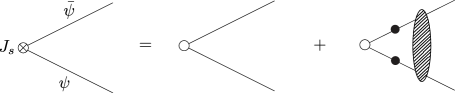
Figure 4: The vertex in interacting theory

Figure 5: The left hand side of the above figure represents a fully quantum corrected two point function. The right hand side expresses the same as a free theory correlation function and its epsilon transform.

Figure 6: The left hand side of the above figure represents a fully quantum corrected three point function in the quasi-fermionic theory. The right side expresses the same as a combination of the free fermionic and the free bosonic correlation functions and their epsilon transform.

Hilbert space interpretation

In Minwalla:2022sef , it was demonstrated that the thermal partition function of CS matter theories at large N can be given a simple Hilbert space interpretation. They showed that the partition function can be understood in terms of an associated ungauged theory Hilbert space subject to a Gauss’ law constraint in CS matter theory. This Hilbert space interpretation is at the level of single and multiparticle fock space and in some sense, the high energy sector. On the other hand currents can be interpreted as bound states and hence can be understood to appear in the low energy sector of Hilbert space. The fact that correlation functions of these currents can be understood from the free theories and the fact that they show anyonic behaviour indicates that for the low energy sector as well there should be some interesting Hilbert space interpretation .

Bosonization, Anyon and Anyonic current

In 2D bosonization, there is a direct map between currents of the fermionic and bosonic theories. In three dimensions, there may not exist a direct map as in this case bosonization is realised through anyonic behaviour. However results in this paper indicate that one might be able to define effective anyonic currents which interpolate between fermionic and bosonic currents. One should as well be able to use these anyonic currents to define some effective Wick contraction to get the correlation functions.

CFT bootstrap in momentum or spinor-helicity variables

Three point function of conserved currents can have three structures

$$\langle J_{s_{1}}J_{s_{2}}J_{s_{3}}\rangle=n_{F}\langle J_{s_{1}}J_{s_{2}}J_{s_{3}}\rangle_{FF}+n_{B}\langle J_{s_{1}}J_{s_{2}}J_{s_{3}}\rangle_{FB}+n_{Odd}\langle J_{s_{1}}J_{s_{2}}J_{s_{3}}\rangle_{odd}.$$ (228)

However solving in spinor helicity and momentum space breaks up things naturally in the following way:

$$\langle J_{s_{1}}J_{s_{2}}J_{s_{3}}\rangle=\left(n_{F}+n_{B}\right)\langle J_{s_{1}}J_{s_{2}}J_{s_{3}}\rangle_{nh}+\left(n_{F}-n_{B}\right)\langle J_{s_{1}}J_{s_{2}}J_{s_{3}}\rangle_{h,even}+n_{odd}\langle J_{s_{1}}J_{s_{2}}J_{s_{3}}\rangle_{h,odd}$$ (229)

where the "nh" peice saturates the WT identity and the coefficient of it is fixed by two point function, whereas the homogeneous piece depends on the OPE coeffcient and contains both parity even and parity odd contributions. Further, using the fact that in spinor helicity variables the homogeneous odd and the homogeneous even parts are related trivially which leads to

$$\langle J_{s_{1}}J_{s_{2}}J_{s_{3}}\rangle=c_{2pt}\langle J_{s_{1}}J_{s_{2}}J_{s_{3}}\rangle_{nh}+c_{s}e^{i\theta}\langle J_{s_{1}}J_{s_{2}}J_{s_{3}}\rangle_{h}.$$ (230)

Now, if we compute the free theory correlators, the homogeneous and non homogeneous parts can be isolated just from say, the free bosonic theory correlator. This gives us a powerful result that the full three point function can just be obtained from just the free bosonic theory or just from the free fermionic theory.

We would like to repeat the same for four point functions, that is write them in the form,

$$\langle J_{s_{1}}J_{s_{2}}J_{s_{3}}J_{s_{4}}\rangle=\langle J_{s_{1}}J_{s_{2}}J_{s_{3}}J_{s_{4}}\rangle_{nh}+\langle J_{s_{1}}J_{s_{2}}J_{s_{3}}J_{s_{4}}\rangle_{h}.$$ (231)

We believe separation of homogeneous and non-homogeneous parts in the four point function would lead to important insights into the structure of four point functions as it did in the case of three point functions. We believe this will lead to an even more beautiful structure in CS matter theory.

It would also be very interesting to develop bootstrapping ideas directly in momentum space or in spinor helicity variables. See Caron-Huot:2021kjy for some progress towards this. A naive analysis is presented below, see also Gandhi:2021gwn .

$\langle TOOO\rangle_{\text{QF}}$

We can use conformal block decomposition to write

$$\begin{split}\langle TOOO\rangle_{\text{QF}}&=\sum_{s}\langle TOJ_{s}\rangle_{\text{QF}}\langle J_{s}OO\rangle_{\text{QF}}\\ &=\sum_{s}\bigg{(}\langle TOJ_{s}\rangle_{\text{FF}}+\tilde{\lambda}\langle TOJ\rangle_{\text{CB}}\bigg{)}\bigg{(}(1+\tilde{\lambda}^{2})\langle J_{s}OO\rangle_{\text{FF}}\bigg{)}\\ &=(1+\tilde{\lambda}^{2})\sum_{s}\bigg{(}\langle TOJ_{s}\rangle_{\text{FF}}\langle J_{s}OO\rangle_{\text{FF}}+\tilde{\lambda}\langle TOJ_{s}\rangle_{\text{CB}}\langle J_{s}OO\rangle_{\text{CB}}\bigg{)}\\ &=(1+\tilde{\lambda}^{2})\bigg{(}\langle TOOO\rangle_{\text{FF}}+\tilde{\lambda}\langle TOOO\rangle_{\text{CB}}\bigg{)}\end{split}$$ (232)

Going from the second to the third line we have used the fact that $\langle J_{s}OO\rangle_{\text{FF}}=\langle J_{s}OO\rangle_{\text{CB}}$

$\langle JJOO\rangle_{\text{QF}}$

Doing the same process for $\langle JJOO\rangle_{QF}$, we can write

$$\begin{split}&\langle JJOO\rangle_{\text{QF}}=\sum_{s}\langle JJJ_{s}\rangle_{\text{QF}}\langle J_{s}OO\rangle_{\text{QF}}\\ &=\sum_{s}\bigg{(}\frac{1}{(1+\tilde{\lambda}^{2})}(\langle JJJ_{s}\rangle_{\text{FF}}+\tilde{\lambda}~{}\epsilon\cdot(\langle JJJ_{s}\rangle_{\text{FF}}-\langle JJJ_{s}\rangle_{\text{CB}})+\tilde{\lambda}^{2}\langle JJJ_{s}\rangle_{\text{CB}})\bigg{)}\bigg{(}(1+\tilde{\lambda}^{2})\langle J_{s}OO\rangle_{\text{FF}}\bigg{)}\\ &=\sum_{s}\langle JJJ_{s}\rangle_{\text{FF}}\langle J_{s}OO\rangle_{\text{FF}}+\tilde{\lambda}~{}\epsilon\cdot\langle JJJ_{s}\rangle_{\text{FF}}\langle J_{s}OO\rangle_{\text{FF}}-\epsilon\cdot\langle JJJ_{s}\rangle_{\text{CB}}\langle J_{s}OO\rangle_{\text{CB}}\\ &+\tilde{\lambda}^{2}\langle JJJ_{s}\rangle_{\text{CB}}\langle J_{s}OO\rangle_{\text{CB}}=\langle JJOO\rangle_{\text{FF}}+\tilde{\lambda}~{}\epsilon\cdot(\langle JJOO\rangle_{\text{FF}}-\langle JJOO\rangle_{\text{CB}})+\tilde{\lambda}^{2}\langle JJOO\rangle_{\text{CB}}\end{split}$$ (233)

Here again, while going from the second to the third line we have used $\langle J_{s}OO\rangle_{FF}=\langle J_{s}OO\rangle_{CB}$. Even though the above analysis is very naive, it gives the same result as we obtained in (21). We have not taken care of the double trace contributions. However, as was explained in the case of scalar four point functions Turiaci:2018nua , these do not contribute. A naive analysis for spinning correlators also suggest the same. It would be very interesting to put these calculations on a firmer footing. Naive analyses for more general cases are discussed in appendix F.

We believe that since spinor-helicity variables give interesting insights into the CFT correlation functions even at the level of three point functions, it would also reveal some interesting structures at the level of the four point functions which have not been understood as of yet in position or Mellin variables. An other attractive feature of the momentum space analysis is its connection to S-matrix bootstrap programme. At the level of three point functions, a detailed relation of flat space amplitudes and CFT correlators appeared in Jain:2022ujj . It would be interesting to understand this connection at the level of the four point function better and thus making a connection to the S-matrix bootstrap.

Supersymmetric extension

For the case of three point functions it was observed Nizami:2013tpa ; Aharony:2019mbc ; Buchbinder:2021qlb that conserved currents have two structures, one parity even and one parity odd. In spinor-helicity variables, this fact can easily be shown, see Jain:2021whr . This just follows from plugging $n_{B}=n_{F}$ in (229). This implies that there will be one non-homogeneous and only one homogeneous odd contribution. In the context of four point functions, it should lead to very simple structures. It would be interesting to understand this both in terms of the higher spin equation as well as the conformal bootstrap perspective in momentum space. See Binder:2021cif for a calculation of four point correlation function for the stress tensor multiplet for ${\mathcal{N}}=6$ susy SBHS theory. Like non-susy case considered in this paper, Binder:2021cif also showed that there is no contact term contributing to four point function using super symmetric localization.

Correlation function under relevant or marginal deformation and at finite tempearture

In this paper we have considered CS matter theories at the conformal fixed point. Three point and four functions results are fully expressible in terms of free theory results. It would be interesting to check if similar conclusions hold true even away from the conformal fixed point. It would also be interesting to understand if at finite temperature similar conclusions can be reached. To start with we can just concentrate on turning on a mass term Jain:2020puw . In this regard we consider a concrete example of determining the two point function $\langle J_{\mu}J_{\nu}\rangle$ of conserved higher spin operators in the free massive bosonic theory where we have deformed the free bosonic theory by introducing the mass term. We start by acting $Q_{\mu\nu}$ on $\langle J_{\alpha}(x_{1})O(x_{2})\rangle$ in position space.

$$\langle\left[Q_{\mu\nu},J_{\alpha}(x_{1})\right]O(x_{2})\rangle_{\text{FMB}}+\langle J_{\alpha}(x_{1})\left[Q_{\mu\nu},O(x_{1})\right]\rangle_{\text{FMB}}=0$$ (234)

Here $\langle...\rangle_{\text{FMB}}$ denotes a correlator in free massive bosonic theory. The algebra in the massive case is the same as in the case of free theory Jain:2020puw . Using the algebra(250) we get the equation

$$\langle\partial_{\mu}\partial_{\nu}\partial_{\alpha}O(x_{1})O(x_{2})\rangle_{\text{FMB}}+g_{\mu\nu}\langle\partial_{\alpha}\square O(x_{1})O(x_{2})\rangle_{\text{FMB}}+\langle\partial_{\mu}T_{\nu\alpha}(x_{1})O(x_{2})\rangle_{\text{FMB}}$$ (235)

$$+\langle\partial_{\alpha}T_{\mu\nu}(x_{1})O(x_{2})\rangle_{\text{FMB}}+\langle J_{\alpha}(x_{1})\partial_{\mu}J_{\nu}(x_{2})\rangle_{\text{FMB}}=0$$ (236)

One important difference between the massless case and the massive one is that for the latter, 2-point functions of different spins may not be zero. Converting this to momentum space we get the equation

$$\begin{split}&p_{1\mu}p_{1\nu}p_{1\alpha}\langle O(p_{1})O(-p_{1})\rangle_{\text{FMB}}+g_{\mu\nu}p_{1\alpha}p_{1}^{2}\langle O(p_{1})O(-p_{1})\rangle_{\text{FMB}}\\ &+p_{1\mu}\langle T_{\nu\alpha}(p_{1})O(-p_{1})\rangle_{\text{FMB}}+p_{1\alpha}\langle T_{\mu\nu}(p_{1})O(-p_{1})\rangle_{\text{FMB}}+p_{2\mu}\langle J_{\alpha}(p_{1})J_{\nu}(-p_{1})\rangle_{\text{FMB}}=0\end{split}$$ (237)

Now, we can compute $\langle O(p_{1})O(-p_{1})\rangle_{\text{FMB}}$ and $\langle T_{\mu\nu}(p_{1})O(-p_{1})\rangle_{\text{FMB}}$ explicitly. Inputting the explicit expression it can be checked that this equation is indeed satisfied Jain:2020puw . It would be an interesting future goal to generalise this for the case of slightly broken higher spin theories and to check that the correlators in the slightly broken theories can be written in terms of the free bosonic, critical fermion correlators and their epsilon transforms.

Derivation of dual of CS-matter theory

The free bosonic or free fermionic theory in three dimensions are dual to Vasiliev Type A or Type B theory. CS matter theory which is a parity violating theory is dual to Vasiliev theory with parity violating $\theta$ term. Given the fact that we are able to derive the correlation functions in the parity violating CS matter theory in terms of free theory, this indicates that there might be a way to write down these parity violating theta deformed theories in terms of Vasiliev-A or Vasileiv-B theories. Recently, in Aharony:2020omh , it was shown how to rewrite the path integral over free theory vector models in d dimensions in terms of path integrals of fields in one higher dimension in AdS space. Since CS matter theory results can be mapped to free theory results, it might turn out that this rewriting of the path integral can be extended for the case of CS matter theory and show how the $\theta$ term arises. One possible difficulty is the fact that position space correlation functions when expressed in terms of free theory results becomes complicated. Also, even though we could express the three point function in terms of just the free fermion theory, the four point function requires both free fermion and crtical bosonic results .

Contact diagram in AdS or double trace contribution

As mentioned above, we could show that the full slightly broken HSEs can be mapped to the FF HSE, CB HSE their combinations or as we defined earlier, an epsilon transformed version of these. In this analysis we did not require any contact diagrams. As mentioned in the main-text, the result reported in the paper solves the SBHS equations but there could be multiple solutions. In principle one can add contact diagrams to our results Turiaci:2018nua ; Silva:2021ece ; Chowdhury:2019kaq . We suspect these contact diagrams would violate the HSEs. However, let us emphasize again that we could solve SBHS equations without requiring contact diagrams.

For scalar four point function in Turiaci:2018nua it was shown explicitly that contact terms are not required. For $\langle JJJJ\rangle$ in Kalloor:2019xjb it was argued that no contact term is required. Our results indicate that, we may not require AdS contact diagrams and hence no double trace contribution os required. The full results are just obtained from single trace contribution. From AdS perspective this would imply existance of sub-AdS locality in the higher spin gauge theories .

Generating functional for correlation function in CS matter theory

Given the simplicity of the results presented in this paper, it would be interesting to find out a generating functional which reproduces all the results. See for three point function for free theories Giombi:2011rz , for four point function in free theories Didenko:2013bj , see also Gerasimenko:2021sxj for recent abstract discussions on interacting theories. It would be interesting to find explicit expression of correlation function for free theories in momentum space for four point functions.

Finite N bootstrap

Reproducing the results presented in this paper from the position space or Melin space bootstrap perspective would be very interesting. Also generalizing the results by taking subleading order in $\mathcal{O}(\frac{1}{N})$ corrections would be an interesting thing to pursue. In Aharony:2018npf it was shown that to obtain CFT data at $\frac{1}{N^{2}}$ we need to know spinning four-point functions $\langle J_{s_{1}}J_{s_{2}}J_{s_{3}}J_{s_{4}}\rangle$. It would be nice to revisit analytic bootstrap program in Aharony:2018npf in light of the results presented in this paper.

Appendix

Appendix A CS matter theory

In the main text we have defined the QF theory. Let us define the QB theory here. The QB theory is two different theories which are dual to each other. These are a boson coupled to the CS gauge field and a critical fermion coupled to the CS gauge field. Here we briefly discuss a boson coupled to the CS gauge field. More details can be found in Aharony:2018pjn .

A.1 Bosonic theory coupled to CS field

The bosonic theory coupled to the Chern-Simons gauge field has the following action

$$S=\int d^{3}x\left[D_{\mu}\bar{\phi}D^{\mu}\phi+i\epsilon^{\mu\nu\rho}\frac{\kappa_{F}}{4\pi}\text{Tr}(A_{\mu}\partial_{\nu}A_{\rho}-\frac{2i}{3}A_{\mu}A_{\nu}A_{\rho})+\frac{(2\pi)^{2}}{\kappa_{B}^{2}}(x_{6}^{B}+1)(\bar{\phi}\phi)^{3}\right]$$ (238)

The scalar primary operator has conformal dimension $\Delta=1+\mathcal{O}\left(\frac{1}{N}\right)$ and is parity even. The spin-1 and spin-2 conserved currents have dimensions 2 and 3 respectively. The theory also has an infinite tower of weakly broken higher spin currents $J_{s}$ with spin $s>2$ and conformal dimension $\Delta=s+1+\mathcal{O}\left(\frac{1}{N}\right)$. In this text we will refer to this as the quasi bosonic(QB) theory.

A.2 Relationship between parameters

The coupling constant in the CS matter theories is defined as follows,

$$\lambda_{b}=\frac{N_{b}}{\kappa_{b}},\quad\lambda_{f}=\frac{N_{f}}{\kappa_{f}}$$ (239)

we now introduce a few other useful variables which will help simplify our expressions. Aharony:2012nh GurAri:2012is

$$\tilde{N}=2N_{b}\frac{\sin\pi\lambda_{b}}{\pi\lambda_{b}}=2N_{f}\frac{\sin\pi\lambda_{f}}{\pi\lambda_{f}}$$ (240)

$$\tilde{\lambda}_{qb}=\tan(\frac{\pi\lambda_{b}}{2})=\cot(\frac{\pi\lambda_{f}}{2})$$ (241)

$$\tilde{\lambda}_{qf}=\cot(\frac{\pi\lambda_{b}}{2})=\tan(\frac{\pi\lambda_{f}}{2})$$ (242)

Appendix B Higher Spin Current Algebra

In theories possessing higher spin symmetry, there exist an infinite tower of conserved currents such that their associated charge $Q_{s}$ kills any correlator. i.e.

$$\sum_{i}\langle J_{s_{1}}...[Q_{s},J_{s_{i}}]..J_{s_{n}}\rangle=0$$ (243)

The conserved charges have an associated algebra with the current operators. We can constrain this algebra from covariance, dimensionality, parity, spin considerations etc. Throughout this text we will be mainly focusing on two charges, namely $Q_{3}$ and $Q_{4}$. For the FB theory we have a scalar operator $O$ with dimension $\Delta=1$ and an infinite tower of exactly conserved currents $J_{s}$ with integer spin $s$ and dimension $\Delta=s+1$. The algebra of charges $Q_{3}$ and $Q_{4}$ with $O$ and $J_{1}$ is given by :

$$[Q_{3},O] =[Q_{\mu\nu},O]=c_{1}\partial_{(\mu}J_{\nu)}$$ (244)

$$[Q_{3},J] =[Q_{\mu\nu},J_{\rho}]=c_{2}\partial_{\mu}\partial_{\nu}\partial_{\rho}O+c_{3}g_{\mu\nu}\partial_{\rho}\Box O+c_{4}\partial_{(\mu}T_{\nu)\rho}+c_{5}\partial_{\rho}T_{\mu\nu}$$ (245)

$$[Q_{4},O] =[Q_{\mu\nu\rho},O]=d_{1}\partial_{\mu}\partial_{\nu}\partial_{\rho}O+d_{2}g_{(\mu\nu}\partial_{\rho)}\square O+d_{3}\partial_{(\mu}T_{\nu\rho)}$$ (247)

$$[Q_{4},J] =[Q_{\mu\nu\rho},J_{\alpha}]=d_{4}\,\partial_{(\mu}\partial_{\nu}\partial_{\rho)}J_{\alpha}+d_{5}\,\partial_{\alpha}\partial_{(\mu}\partial_{\nu}J_{\rho)}+d_{6}g_{(\mu\nu}\partial_{\rho)}\Box J_{\alpha}$$ (248)

$$\hskip 71.13188pt+d_{7}g_{\mu\nu}\partial_{\alpha}\Box J_{\rho}+d_{8}g_{\alpha(\mu}\partial_{\nu}\Box J_{\rho)}+d_{9}\partial_{\alpha}J_{(\mu\nu\rho)}$$ (249)

The several constants $\{c_{i},d_{j}\}$ can be fixed by using two-point and three-point functions. Similarly the FF theory in three dimensions has a pseudo-scalar operator $O$ with dimension $\Delta=2$ and an infinite tower of exactly conserved currents $J_{s}$ with integer spin $s$ and dimension $\Delta=s+1$. The algebra of charges $Q_{3}$ and $Q_{4}$ with $O$ and $J_{1}$ is as follows :

$$[Q_{\mu\nu},O] =\epsilon_{\mu ab}\,\partial^{a}\partial_{\nu}J^{b}$$ (250)

$$[Q_{\mu\nu},J_{\rho}] =\epsilon_{\sigma\rho(\mu}\partial_{\nu)}\partial_{\sigma}O+i\partial_{(\mu}T_{\nu)\rho}+\partial_{\rho}T_{\mu\nu}$$ (251)

$$[Q_{\mu\nu},T_{\alpha\beta}] =p_{\mu}p_{\nu}p_{\alpha}J_{\beta}+p_{\mu}p_{\beta}p_{\alpha}J_{\nu}+g_{\mu\nu}p_{\alpha}p_{1}^{2}J_{\beta}+p_{\mu}J_{\nu\alpha\beta}$$ (252)

$$[Q_{\mu\nu\rho},O] =\partial_{\mu}\partial_{\nu}\partial_{\rho}O+g_{\mu\nu}\partial_{\rho}\Box O+\epsilon_{\mu ab}\partial_{\nu}\partial_{a}T_{b\rho}$$ (254)

$$[Q_{\mu\nu\rho},J_{\alpha}] =a\,\partial_{(\mu}\partial_{\nu}\partial_{\rho)}J_{\alpha}+b\,\partial_{\alpha}\partial_{(\mu}\partial_{\nu}J_{\rho)}+\partial_{\alpha}J_{(\mu\nu\rho)}$$ (255)

$$\hskip 8.5359pt+g_{(\mu\nu}\partial_{\rho)}\Box J_{\alpha}+g_{\mu\nu}\partial_{\alpha}\Box J_{\rho}+cg_{\alpha(\mu}\partial_{\nu}\Box J_{\rho)}$$ (256)

$$[Q_{\mu\nu\rho},T_{\alpha\beta}] =b_{1}\partial_{\mu}\partial_{\nu}\partial_{\rho}T_{\alpha\beta}+b_{2}\partial_{\mu}\partial_{\nu}\partial_{\alpha}T_{\rho\beta}+b_{3}\partial_{\mu}J_{\nu\rho\alpha\beta}+b_{4}\partial_{\alpha}J_{\mu\nu\rho\beta}$$ (257)

In the case of theories with slightly broken higher spin symmetry, the non-conservation equation gets a contribution proportional to the coupling strength $\tilde{\lambda}$ and becomes,

$$\sum_{i}\langle J_{s_{1}}...[Q_{s},J_{s_{i}}]..J_{s_{n}}\rangle=\int\langle\partial\cdot J_{s}J_{s_{1}}...J_{s_{n}}\rangle$$ (258)

The non-conservation for the currents $J_{3}$ and $J_{4}$ for the QB theory is given by Maldacena:2012sf ; Giombi:2016zwa ,

$$\partial\cdot J_{3} =\partial_{\sigma}J^{\sigma}_{\mu\nu}(x)=\epsilon_{\mu ab}\big{(}f_{0}J_{a}(x)\partial_{b}\partial_{\nu}O(x)+b_{1}\partial_{b}J_{a}(x)\partial_{\nu}O(x)$$ (259)

$$\hskip 85.35826pt+f_{1}\partial_{\nu}J_{a}(x)\partial_{b}O(x)+b_{2}O(x)\partial_{b}\partial_{\nu}J_{a}(x)\big{)}$$ (260)

$$\partial\cdot J_{4} =\partial_{\sigma}J^{\sigma}_{\mu\nu\rho}(x)=\epsilon_{\mu ab}\big{(}f_{0}T_{a\nu}(x)\partial_{b}\partial_{\rho}O(x)+b_{1}\partial_{b}T_{a\nu}(x)\partial_{\rho}O(x)$$ (261)

$$\hskip 91.04872pt+f_{1}\partial_{\rho}T_{a\nu}(x)\partial_{b}O(x)+b_{2}O(x)\partial_{b}\partial_{\rho}T_{a\nu}(x)\big{)}$$ (262)

and in the case of QF theories, the non-conservation for $J_{3}$ and $J_{4}$ are given by

$$\partial_{\sigma}J^{\sigma}_{\mu\nu} =a\partial_{(\mu}J_{\nu)}O+bJ_{(\nu}\partial_{\mu)}O$$ (263)

$$\partial_{\sigma}J^{\sigma}_{\mu\nu\rho} =r_{0}\partial_{\mu}O(x)T_{\nu\rho}(x)+\epsilon_{\mu ab}\big{(}a_{0}J_{a}(x)\partial_{\rho}\partial_{\nu}J_{b}(x)+b_{1}J_{a}(x)\partial_{b}\partial_{\nu}J_{\rho}(x)+e_{0}J_{\nu}(x)\partial_{a}\partial_{\rho}J_{b}(x)\big{)}$$ (264)

here the several factors $\{f_{i},b_{j}\}$ are no longer constants but pick up a $\tilde{\lambda}$ dependence. The precise values are given as follows,

$$a=\frac{3}{5\tilde{N}}\frac{\tilde{\lambda}}{1+\tilde{\lambda}^{2}},\quad b=-\frac{2}{5\tilde{N}}\frac{\tilde{\lambda}}{1+\tilde{\lambda}^{2}},\quad$$ (265)

$$r_{0}=\frac{480}{7\tilde{N}}\frac{\tilde{\lambda}}{1+\tilde{\lambda}^{2}},\quad b_{1}=-\frac{512}{3\tilde{N}}\frac{\tilde{\lambda}}{1+\tilde{\lambda}^{2}},\quad b_{2}=\frac{128}{3\tilde{N}}\frac{\tilde{\lambda}}{1+\tilde{\lambda}^{2}}$$ (266)

$$f_{0}=\frac{64}{\tilde{N}}\frac{\tilde{\lambda}}{1+\tilde{\lambda}^{2}},\quad f_{1}=-\frac{128}{3\tilde{N}}\frac{\tilde{\lambda}}{1+\tilde{\lambda}^{2}}$$ (267)

The algebra for the slightly broken HS theory is also slightly modified where the coefficients may or may not pick up a dependence of the coupling constant. The modified algebra for each theory is given by,
Quasi-bosonic theory

$$[Q_{3},O] =[Q_{\mu\nu},O]=c_{1}\partial_{(\mu}J_{\nu)}$$ (268)

$$[Q_{3},J] =[Q_{\mu\nu},J_{\rho}]=c_{2}\partial_{\mu}\partial_{\nu}\partial_{\rho}O+c_{3}g_{\mu\nu}\partial_{\rho}\Box O+c_{4}\partial_{(\mu}T_{\nu)\rho}+c_{5}\partial_{\rho}T_{\mu\nu}$$ (269)

$$[Q_{4},O] =[Q_{\mu\nu\rho},O]=d_{1}\partial_{\mu}\partial_{\nu}\partial_{\rho}O+d_{2}g_{(\mu\nu}\partial_{\rho)}\square O+d_{3}\partial_{(\mu}T_{\nu\rho)}$$ (271)

$$[Q_{4},J] =[Q_{\mu\nu\rho},J_{\alpha}]=d_{4}\,\partial_{(\mu}\partial_{\nu}\partial_{\rho)}J_{\alpha}+d_{5}\,\partial_{\alpha}\partial_{(\mu}\partial_{\nu}J_{\rho)}+d_{6}g_{(\mu\nu}\partial_{\rho)}\Box J_{\alpha}$$ (272)

$$\hskip 71.13188pt+d_{7}g_{\mu\nu}\partial_{\alpha}\Box J_{\rho}+d_{8}g_{\alpha(\mu}\partial_{\nu}\Box J_{\rho)}+d_{9}\partial_{\alpha}J_{(\mu\nu\rho)}$$ (273)

Quasi-fermionic theory

$$[Q_{\mu\nu},O] =c_{1}\epsilon_{\mu ab}\,\partial^{a}\partial_{\nu}J^{b}$$ (274)

$$[Q_{\mu\nu},J_{\rho}] =\frac{1}{1+\tilde{\lambda}^{2}}c_{2}\epsilon_{\sigma\rho(\mu}\partial_{\nu)}\partial_{\sigma}O+c_{3}\partial_{(\mu}T_{\nu)\rho}+c_{4}\partial_{\rho}T_{\mu\nu}$$ (275)

$$[Q_{\mu\nu\rho},O] =a_{1}\partial_{\mu}\partial_{\nu}\partial_{\rho}O+a_{2}g_{\mu\nu}\partial_{\rho}\Box O+a_{3}\epsilon_{\mu ab}\partial_{\nu}\partial_{a}T_{b\rho}$$ (277)

$$[Q_{\mu\nu\rho},J_{\alpha}] =b_{1}\,\partial_{(\mu}\partial_{\nu}\partial_{\rho)}J_{\alpha}+b_{2}\,\partial_{\alpha}\partial_{(\mu}\partial_{\nu}J_{\rho)}+b_{3}\partial_{\alpha}J_{(\mu\nu\rho)}$$ (278)

$$\hskip 8.5359pt+g_{(\mu\nu}\partial_{\rho)}\Box J_{\alpha}+g_{\mu\nu}\partial_{\alpha}\Box J_{\rho}+cg_{\alpha(\mu}\partial_{\nu}\Box J_{\rho)}$$ (279)

$$[Q_{\mu\nu\rho},T_{\alpha\beta}] =b_{1}\partial_{\mu}\partial_{\nu}\partial_{\rho}T_{\alpha\beta}+b_{2}\partial_{\mu}\partial_{\nu}\partial_{\alpha}T_{\rho\beta}+b_{3}\partial_{\mu}J_{\nu\rho\alpha\beta}+b_{4}\partial_{\alpha}J_{\mu\nu\rho\beta}$$ (280)

the precise values of all the $\{a_{i},b_{j},c_{k}\}$ sometimes cannot be determined but it is usually not required. The only information we know about these coefficients is if they are modified for SBHS theories. Our aim in this paper has been to map the correlation function in SBHS theories to the free theories which does not require explicit knowledge of these coefficients . If we now move to lightcone coordinates, these coeffcients are explicitly known and can be found in Maldacena:2012sf ; Jain:2020puw .

Appendix C Spinor helicity variables

Spinor-helicity variables are a useful tool to represent scattering amplitudes and correlation functions in a compact manner. Here we will give a short introduction of the basic definitions and list the identities which we used throughout the text. For a more detailed discussion see Maldacena:2011nz .

We begin by expressing the 4-momentum as,

$$p_{\alpha\dot{\alpha}}=\lambda_{\alpha}\tilde{\lambda}_{\dot{\alpha}}$$ (284)

We define barred spinors using,

$$\bar{\lambda}_{\alpha}=\tilde{\lambda}_{\dot{\alpha}}\tau^{\dot{\alpha}}_{\alpha}\quad\text{where\quad}\tau^{\dot{\alpha}}_{\alpha}=-\epsilon^{\dot{\alpha}\dot{\beta}}\mathbb{I}_{\dot{\beta}\alpha}$$ (285)

The 3-momentum can be expressed as

$$p^{i}=\frac{1}{2}(\sigma^{i})^{\alpha}_{\hphantom{\alpha}\beta}\lambda_{\alpha}\bar{\lambda}^{\beta}$$ (286)

Using the above relations we can express the momentum derivatives in terms of spinorial derivatives and the special conformal generator then becomes

$$K^{\kappa}=2\sum_{i=1}^{n}(\sigma^{\kappa})_{\alpha}^{\hphantom{\alpha}\beta}\frac{\partial^{2}}{\partial\lambda_{i\alpha}\partial\lambda_{i}^{\beta}}$$ (287)

We also define the inner product brackets as follows,

$$\langle ij\rangle=\epsilon^{\alpha\beta}\lambda_{i\alpha}\lambda_{j\beta}\enspace,\;\langle i\bar{j}\rangle=\epsilon^{\alpha\beta}\lambda_{i\alpha}\bar{\lambda}_{j\beta}$$ (288)

Finally we define the transverse polarization vectors as,

$$z_{\alpha\beta}^{-}=\frac{\lambda_{\alpha}\lambda_{\beta}}{2p}\quad\quad z_{\alpha\beta}^{+}=\frac{\bar{\lambda}_{\alpha}\bar{\lambda}_{\beta}}{2p}$$ (289)

Given a momentum space expression we dot it with the polarization tensors to convert it into spinor-helicity notation. For example

$$z_{i}\cdot p_{j}=-\frac{\langle ij\rangle\langle i\bar{j}\rangle}{2p_{i}}\quad\quad z_{i}\cdot z_{j}=-\frac{\langle ij\rangle^{2}}{4p_{i}p_{j}}$$ (290)

When we have three momenta, the spinor brackets satisfy the following relations: Baumann:2020dch

$$\langle ba\rangle\langle\bar{a}\bar{c}\rangle =E\langle b\bar{c}\rangle$$ (291)

$$\langle ba\rangle\langle\bar{a}c\rangle =(E-2k_{c})\langle bc\rangle$$ (292)

$$\langle\bar{b}a\rangle\langle\bar{a}\bar{c}\rangle =(E-2k_{b})\langle\bar{b}\bar{c}\rangle$$ (293)

$$\langle\bar{b}a\rangle\langle\bar{a}c\rangle =(E-2k_{b}-2k_{c})\langle\bar{b}c\rangle$$ (294)

$$\langle ba\rangle\langle\bar{a}b\rangle+\langle bc\rangle\langle\bar{c}b\rangle =0$$ (295)

$$\langle ab\rangle\langle\bar{a}\bar{b}\rangle =E(E-2k_{c})$$ (296)

$$\langle\bar{b}a\rangle\langle\bar{a}b\rangle =(E-2k_{a})(E-2k_{b})=k_{c}^{2}-(k_{a}-k_{b})^{2}$$ (297)

Similarly, when we have four momenta we have the following identities

$$\langle ba\rangle\langle\bar{a}\bar{c}\rangle+\langle bd\rangle\langle\bar{d}\bar{c}\rangle =E\langle b\bar{c}\rangle$$ (298)

$$\langle ba\rangle\langle\bar{a}c\rangle+\langle bd\rangle\langle\bar{d}c\rangle =(E-2k_{c})\langle bc\rangle$$ (299)

$$\langle\bar{b}a\rangle\langle\bar{a}\bar{c}\rangle+\langle\bar{b}d\rangle\langle\bar{d}\bar{c}\rangle =(E-2k_{b})\langle\bar{b}\bar{c}\rangle$$ (300)

$$\langle\bar{b}a\rangle\langle\bar{a}c\rangle+\langle\bar{b}d\rangle\langle\bar{d}c\rangle =(E-2k_{b}-2k_{c})\langle\bar{b}c\rangle$$ (301)

$$\langle ba\rangle\langle\bar{a}b\rangle+\langle bc\rangle\langle\bar{c}b\rangle+\langle bd\rangle\langle\bar{d}b\rangle =0$$ (302)

$$\langle ba\rangle\langle\bar{a}\bar{b}\rangle-\langle cd\rangle\langle\bar{d}\bar{c}\rangle =E(2k_{c}+2k_{d}-E)$$ (303)

$$\langle\bar{b}a\rangle\langle\bar{a}b\rangle-\langle\bar{c}d\rangle\langle\bar{d}c\rangle =(k_{c}-k_{b})^{2}-(k_{a}-k_{b})^{2}$$ (304)

In our computation we also made use of the expression of dot products of momenta with each other and with null transverse polarization vectors $z_{i}$ which satisfy the null condition $z_{i}^{2}=0$ and the transverse condition $z_{i}\cdot p_{i}=0$. The dot products take the following form

Parity Even:

$$2p_{a}\cdot p_{b}=-\langle ab\rangle\langle\bar{a}\bar{b}\rangle,\quad 2p_{a}\cdot z_{b}^{+}=\frac{\langle a\bar{b}\rangle\langle\bar{b}\bar{a}\rangle}{2p_{b}},\quad 2p_{a}\cdot z_{b}^{-}=\frac{\langle\bar{a}b\rangle\langle ba\rangle}{2p_{b}}$$ (305)

$$2z_{a}^{+}\cdot z_{b}^{+}=-\frac{\langle\bar{a}\bar{b}\rangle^{2}}{4p_{a}p_{b}},\quad 2z_{a}^{-}\cdot z_{b}^{-}=-\frac{\langle ab\rangle^{2}}{4p_{a}p_{b}},\quad 2z_{a}^{+}\cdot z_{b}^{-}=-\frac{\langle\bar{a}b\rangle^{2}}{4p_{a}p_{b}}$$ (306)

Parity Odd:

$$\epsilon_{p_{i}p_{j}z^{+}_{k}} =\frac{-1}{p_{k}}\big{(}\langle i\bar{k}\rangle\langle\bar{k}\bar{j}\rangle+p_{j}\langle i\bar{k}\rangle\langle\bar{k}\bar{i}\rangle+p_{i}\langle j\bar{k}\rangle\langle\bar{k}\bar{j}\rangle\big{)}$$ (307)

$$\epsilon_{p_{i}z^{+}_{j}z^{+}_{k}} =\frac{-1}{p_{j}p_{k}}(\langle i\bar{k}\rangle\langle\bar{k}\bar{j}\rangle\langle j\bar{i}\rangle-p_{i}\langle\bar{j}\bar{k}\rangle^{2})$$ (308)

$$\epsilon_{p_{i}z^{-}_{j}z^{+}_{k}} =\frac{-1}{p_{j}p_{k}}(-\langle i\bar{k}\rangle\langle j\bar{k}\rangle\langle j\bar{i}\rangle-p_{i}\langle j\bar{k}\rangle^{2})$$ (309)

Appendix D Epsilon transforms in spinor-helicity variables

We denote the epsilon transform of an object $X$ as follows

$$\epsilon\cdot X_{\mu\nu\alpha_{1}...\alpha_{n}}=\frac{\epsilon_{(\mu ab}p_{a}}{p}X_{b\nu)\alpha_{1}...\alpha_{n}}$$ (311)

We illustrate the epsilon transform by an example. Consider the expression of $\langle JJO\rangle_{\text{odd}}$ in the quasi-bosonic theory

$$\langle J_{\alpha}(p_{1})J_{\nu}(p_{2})O(p_{3})\rangle_{\text{odd}}=\frac{\epsilon_{\alpha ab}\,p_{1a}}{p_{1}}\langle J_{b}(p_{1})J_{\nu}(p_{2})O(p_{3})\rangle_{\text{FB}}$$ (312)

The explicit expression of $\langle JJO\rangle_{\text{FB}}$ is given by,

$$\langle J_{\alpha}(p_{1})J_{\nu}(p_{2})O(p_{3})\rangle_{\text{FB}}=\pi_{\mu a}(p_{1})\pi_{\nu b}(p_{2})\big{(}A(p_{i})p_{2a}p_{1b}+B(p_{i})\delta_{ab}\big{)}$$ (313)

If we dot it with the polarization tensors $z^{-}_{1\mu},z^{-}_{2\nu}$ on both sides we will get

$$\langle J_{-}J_{-}O(p_{3})\rangle_{\text{FB}} =\frac{A\langle 1,2\rangle^{2}\left\langle 1,\bar{2}\right\rangle\left\langle 2,\bar{1}\right\rangle}{8p_{1}p_{2}}+\frac{B\langle 1,2\rangle^{2}}{2p_{1}p_{2}}$$ (314)

$$\langle J_{-}J_{-}O(p_{3})\rangle_{\text{odd}} =i\frac{A\langle 1,2\rangle^{2}\left\langle 1,\bar{2}\right\rangle\left\langle 2,\bar{1}\right\rangle}{8p_{1}p_{2}}+i\frac{B\langle 1,2\rangle^{2}}{2p_{1}p_{2}}$$ (315)

hence we have $\langle\epsilon\cdot JJO\rangle_{\text{FB}}\rightarrow i\langle JJO\rangle_{\text{FB}}$. Similarly if we dot with $z^{+}_{1\mu},z^{+}_{2\nu}$ on both sides we will get

$$\langle J_{-}J_{-}O(p_{3})\rangle_{\text{FB}} =\frac{A\left\langle 1,\bar{2}\right\rangle\left\langle 2,\bar{1}\right\rangle\left\langle\bar{1},\bar{2}\right\rangle^{2}}{16p_{1}p_{2}}+\frac{B\left\langle\bar{1},\bar{2}\right\rangle^{2}}{8p_{1}p_{2}}$$ (316)

$$\langle J_{-}J_{-}O(p_{3})\rangle_{\text{odd}} =-i\frac{A\left\langle 1,\bar{2}\right\rangle\left\langle 2,\bar{1}\right\rangle\left\langle\bar{1},\bar{2}\right\rangle^{2}}{16p_{1}p_{2}}-i\frac{B\left\langle\bar{1},\bar{2}\right\rangle^{2}}{8p_{1}p_{2}}$$ (317)

so we notice $\langle\epsilon\cdot JJO\rangle_{\text{FB}}\rightarrow-i\langle JJO\rangle_{\text{FB}}$. Thus we notice that in spinor-heilcity variables $\langle\epsilon\cdot JJO\rangle_{\text{FB}}\rightarrow\pm i\langle JJO\rangle_{\text{FB}}$

It turns out that this observation is not limited to just $\langle JJO\rangle$ and in-fact for any correlator we have $\langle\epsilon\cdot J_{s_{1}}J_{s_{2}}J_{s_{3}}\rangle\rightarrow\pm i\langle J_{s_{1}}J_{s_{2}}J_{s_{3}}\rangle$. The analogous result for four-point functions holds true as well.

Appendix E Two-point functions

In this section, we use the SBHS equation to calculate the two point functions. We present a simple example and demonstrate how higher spin symmetry can be employed to calculate correlation functions.

E.1 $\langle JJ\rangle_{\text{QF}}$

Consider the action of $Q_{3}$ on the correlator $\langle J_{\alpha}O\rangle$ in the QF theory,

$$[Q_{\mu\nu},\langle J_{\alpha}(x_{1})O(x_{2})\rangle_{\text{QF}}]=\int_{x}\langle\partial_{\sigma}J^{\sigma}_{(\mu\nu)}(x)J_{\alpha}(x_{1})O(x_{2})\rangle_{\text{QF}}$$ (318)

Using (274) and (275) we expand the LHS as follows

$$[Q_{\mu\nu},\langle J_{\alpha}(x_{1})O(x_{2})\rangle_{\text{QF}}]=\langle[Q_{\mu\nu},J_{\alpha}(x_{1})]O(x_{2})\rangle_{\text{QF}}+\langle J_{\alpha}(x_{1})[Q_{\mu\nu},O(x_{2})]\rangle_{\text{QF}}$$ (319)

$$=c_{2}\epsilon_{\sigma\rho(\mu}\partial_{1\nu)}\partial_{\sigma}\langle O(x_{1})O(x_{2})\rangle_{\text{QF}}+c_{3}\partial_{(1\mu}\langle T_{\nu)\rho}(x_{1})O(x_{2})\rangle_{\text{QF}}+c_{4}\partial_{1\rho}\langle T_{\mu\nu}(x_{1})O(x_{2})\rangle_{\text{QF}}$$ (320)

$$+c_{1}\epsilon_{\mu ab}\,\partial^{1a}\partial_{1\nu}\langle J^{b}(x_{1})O(x_{2})\rangle_{\text{QF}}$$ (321)

Now using the fact that $\langle J_{s}O\rangle$ is zero, the LHS simplifies to just two terms

$$c_{2}\epsilon_{\sigma\rho(\mu}\partial_{1\nu)}\partial_{1\sigma}\langle O(x_{1})O(x_{2})\rangle_{\text{QF}}+c_{1}\epsilon_{\mu ab}\,\partial^{1a}\partial_{1\nu}\langle J_{\alpha}(x_{1})J^{b}(x_{2})\rangle_{\text{QF}}$$ (322)

Now, using the non-conservation of $J_{3}$ from (263) we can write the RHS as,

$$\int_{x}\langle\partial_{\sigma}J^{\sigma}_{(\mu\nu)}(x)J_{\alpha}(x_{1})O(x_{2})\rangle_{\text{QF}} =\int_{x}\langle(a\partial_{(\mu}J_{\nu)}(x)O(x)+bJ_{(\nu}(x)\partial_{\mu)}O(x))J_{\alpha}(x_{1})O(x_{2})\rangle_{\text{QF}}$$ (323)

$$=\int_{x}(a-b)\langle\partial_{(\mu}J_{\nu)}(x)O(x)J_{\alpha}(x_{1})O(x_{2})\rangle_{\text{QF}}$$ (324)

$$=\int_{x}(a-b)\langle\partial_{(\mu}J_{\nu)}(x)J_{\alpha}(x_{1})\rangle_{\text{QF}}\langle O(x)O(x_{2})\rangle_{\text{QF}}$$ (325)

where in the second line we used integration by parts and in the third line we wrote the only nonzero large-$\tilde{N}$ contribution.

Now, to get rid of the integral and to make the overall HSE simpler we write it in momentum space as follows

$$c_{2}\epsilon_{\sigma\rho(\mu}p_{1\nu)}p_{1\sigma}\langle O(p_{1})O(-p_{1})\rangle_{\text{QF}}+c_{1}\epsilon_{\mu ab}p^{1a}p_{1\nu}\langle J_{\alpha}(p_{1})J^{b}(-p_{1})\rangle_{\text{QF}}$$ (326)

$$=16i\frac{\tilde{\lambda}}{1+\tilde{\lambda}^{2}}p_{1(\mu}\langle J_{\nu)}(-p_{1})J_{\alpha}(p_{1})\rangle_{\text{QF}}\langle O(p_{1})O(-p_{1})\rangle_{\text{QF}}$$ (327)

where we used the values for $a,b$ from (281). Thus, we have an expression for the unknown correlator $\langle JJ\rangle_{\text{QF}}$ and now we will try to solve for it. The scalar 2-point function in the QF theory is given by,

$$\langle O(p)O(-p)\rangle_{\text{QF}}=\frac{\tilde{N}}{2}(1+\tilde{\lambda}^{2})\langle O(p)O(-p)\rangle_{\text{FF}}=-\frac{\tilde{N}}{2}(1+\tilde{\lambda}^{2})\frac{p}{8}$$ (328)

while the $\langle JJ\rangle_{\text{QF}}$ correlator decomposes as follows,

$$\langle J_{\mu}(p)J_{\nu}(-p)\rangle_{\text{QF}} =\frac{\tilde{N}}{2}[\langle J_{\mu}(p)J_{\nu}(-p)\rangle_{\text{even}}+\langle J_{\mu}(p)J_{\nu}(-p)\rangle_{\text{odd}}]$$ (329)

$$=\frac{\tilde{N}}{2}\left[\frac{p_{\mu}p_{\nu}-p^{2}g_{\mu\nu}}{16p}+\tilde{c}_{JJ}\epsilon_{\mu\nu a}p^{a}\right]$$ (330)

where the even part of the correlator is just the FF correlator and for the odd part we make a guess knowing that the term should be parity odd and have the correct dimensions which leaves only one possibility. Substituting (328) and (329) back in (326) and equating the parity odd tensor structures we get

$$\tilde{c}_{JJ}=\frac{\tilde{\lambda}}{16}$$ (331)

Thus, we see that the above expression for $\langle JJ\rangle_{\text{QF}}$ matches with what we had earlier. Now, using the definition of $\tilde{N}$ and $\tilde{\lambda}$ from (2) let us rewrite the expression in a different way,

$$\langle J_{\mu}(p)J_{\nu}(-p)\rangle_{\text{QF}} =\frac{\tilde{N}}{2}\left[\frac{p_{\mu}p_{\nu}-p^{2}g_{\mu\nu}}{16p}+\frac{\tilde{\lambda}}{16}\epsilon_{\mu\nu a}p^{a}\right]$$ (332)

$$=N_{f}\frac{\sin\pi\lambda_{f}}{\pi\lambda_{f}}\left[\frac{p_{\mu}p_{\nu}-p^{2}g_{\mu\nu}}{16p}+\frac{\tan(\frac{\pi\lambda_{f}}{2})}{16}\epsilon_{\mu\nu a}p^{a}\right]$$ (333)

If we now dot with the polarization tensors $z_{1\mu},z_{2\nu}$ and convert to spinor-helicity variables, we will get

$$z_{1\mu}z_{2\nu}\langle J_{\mu}(p)J_{\nu}(-p)\rangle_{\text{QF}} =N_{f}\frac{\sin\pi\lambda_{f}}{\pi\lambda_{f}}\left[\frac{-pz_{1}\cdot z_{2}}{16p}+\frac{\tan(\frac{\pi\lambda_{f}}{2})}{16}\epsilon_{z_{1}z_{2}p}\right]$$ (334)

$$=-\frac{iNe^{i\pi\lambda_{f}}\langle 12\rangle^{2}}{32\pi\lambda_{f}p}$$ (335)

Thus we see that in spinor-helicity variables, the two-point function turns out to be just the free theory expression but with an overall phase factor. This procedure can be generalised for arbitrary spin-s conserved currents.

Appendix F Naive conformal bootstrapping and conformal block decomposition

In this section we present a naive conformal block decomposition of the four point function. In the discussion section we presented a naive analysis for $\langle TOOO\rangle_{\text{QF}}$ and $\langle JJOO\rangle_{\text{QF}}.$ In the following we consider two more cases of interest.

F.1 $\langle JJTO\rangle_{\text{QF}}$

$$\begin{split}&\langle JJTO\rangle_{\text{QF}}=\sum_{s}\langle JJJ_{s}\rangle_{\text{QF}}\langle J_{s}TO\rangle_{\text{QF}}\\ &=\sum_{s}\bigg{(}\frac{1}{1+\tilde{\lambda}^{2}}(\langle JJJ_{s}\rangle_{\text{FF}}+\tilde{\lambda}~{}\epsilon\cdot(\langle JJJ_{s}\rangle_{\text{FF}}-\langle JJJ_{s}\rangle_{\text{CB}})+\tilde{\lambda}^{2}\langle JJJ_{s}\rangle_{\text{CB}})\bigg{)}\bigg{(}\langle J_{s}TO\rangle_{\text{FF}}+\tilde{\lambda}\langle J_{s}TO\rangle_{\text{CB}}\bigg{)}\\ &=\frac{1}{1+\tilde{\lambda}^{2}}\sum_{s}\bigg{(}\langle JJJ_{s}\rangle_{\text{FF}}\langle J_{s}TO\rangle_{\text{FF}}+\tilde{\lambda}\langle JJJ_{s}\rangle_{\text{FF}}\langle J_{s}TO\rangle_{\text{CB}}+\tilde{\lambda}(\epsilon\cdot\langle JJJ_{s}\rangle_{\text{FF}})\langle J_{s}TO\rangle_{\text{FF}}\\ &+\tilde{\lambda}^{2}(\epsilon\cdot\langle JJJ_{s}\rangle_{\text{FF}})\langle J_{s}TO\rangle_{\text{CB}}-\tilde{\lambda}(\epsilon\cdot\langle JJJ_{s}\rangle_{\text{CB}})\langle J_{s}TO\rangle_{\text{FF}}-\tilde{\lambda}^{2}(\epsilon\cdot\langle JJJ_{s}\rangle_{\text{CB}})\langle J_{s}TO\rangle_{\text{CB}}\\ &+\tilde{\lambda}^{2}\langle JJJ_{s}\rangle_{\text{CB}}\langle J_{s}TO\rangle_{\text{FF}}+\tilde{\lambda}^{3}\langle JJJ_{s}\rangle_{\text{CB}}\langle J_{s}TO\rangle_{\text{CB}}\bigg{)}\end{split}$$ (336)

Now, we can use

$$\langle J_{s}TO\rangle_{\text{FF}}=\epsilon\cdot\langle J_{s}TO\rangle_{\text{CB}}~{}~{}\text{and}~{}~{}\langle J_{s}TO\rangle_{\text{CB}}=-\epsilon\cdot\langle J_{s}TO\rangle_{\text{FF}}$$ (337)

If we input this into (336), we get

$$\begin{split}&\frac{1}{1+\tilde{\lambda}^{2}}\sum_{s}\bigg{(}\langle JJJ_{s}\rangle_{\text{FF}}\langle J_{s}TO\rangle_{\text{FF}}-\tilde{\lambda}\langle JJJ_{s}\rangle_{\text{FF}}(\epsilon\cdot\langle J_{s}TO\rangle_{\text{FF}})+\tilde{\lambda}(\epsilon\cdot\langle JJJ_{s}\rangle_{\text{FF}})\langle J_{s}TO\rangle_{\text{FF}}\\ &-\tilde{\lambda}^{2}(\epsilon\cdot\langle JJJ_{s}\rangle_{\text{FF}})(\epsilon\cdot\langle J_{s}TO\rangle_{\text{FF}})-\tilde{\lambda}(\epsilon\cdot\langle JJJ_{s}\rangle_{\text{CB}})(\epsilon\cdot\langle J_{s}TO\rangle_{\text{CB}})-\tilde{\lambda}^{2}(\epsilon\cdot\langle JJJ_{s}\rangle_{\text{CB}})\langle J_{s}TO\rangle_{\text{CB}}\\ &+\tilde{\lambda}^{2}\langle JJJ_{s}\rangle_{\text{CB}}(\epsilon\cdot\langle J_{s}TO\rangle_{\text{CB}})+\tilde{\lambda}^{3}\langle JJJ_{s}\rangle_{\text{CB}}\langle J_{s}TO\rangle_{\text{CB}}\bigg{)}\end{split}$$ (338)

Schematically, we write $(\epsilon\cdot\langle JJJ_{s}\rangle)(\epsilon\cdot\langle J_{s}TO\rangle)$ as $\pm\langle JJJ_{s}\rangle\langle J_{s}TO\rangle$. Thus the above equation becomes

$$\frac{1}{1+\tilde{\lambda}^{2}}\sum_{s}\bigg{(}\langle JJJ_{s}\rangle_{\text{FF}}\langle J_{s}TO\rangle_{\text{FF}}-\tilde{\lambda}\langle JJJ_{s}\rangle_{\text{FF}}(\epsilon\cdot\langle J_{s}TO\rangle_{\text{FF}})+\tilde{\lambda}(\epsilon\cdot\langle JJJ_{s}\rangle_{\text{FF}})\langle J_{s}TO\rangle_{\text{FF}}$$ (339)

$$\hskip 28.45274pt\mp\tilde{\lambda}^{2}(\langle JJJ_{s}\rangle_{\text{FF}})(\langle J_{s}TO\rangle_{\text{FF}})\mp\tilde{\lambda}(\langle JJJ_{s}\rangle_{\text{CB}})(\langle J_{s}TO\rangle_{\text{CB}})-\tilde{\lambda}^{2}(\epsilon\cdot\langle JJJ_{s}\rangle_{\text{CB}})\langle J_{s}TO\rangle_{\text{CB}}$$

$$\hskip 28.45274pt+\tilde{\lambda}^{2}\langle JJJ_{s}\rangle_{\text{CB}}(\epsilon\cdot\langle J_{s}TO\rangle_{\text{CB}})+\tilde{\lambda}^{3}\langle JJJ_{s}\rangle_{\text{CB}}\langle J_{s}TO\rangle_{\text{CB}}\bigg{)}$$

$$=\frac{1}{1+\tilde{\lambda^{2}}}\bigg{(}\langle JJTO\rangle_{\text{FF}}-\tilde{\lambda}~{}\epsilon\cdot\langle JJTO\rangle_{\text{FF}}+\tilde{\lambda}~{}\epsilon\cdot\langle JJTO\rangle_{\text{FF}}\mp\tilde{\lambda}^{2}\langle JJTO\rangle_{\text{FF}}$$

$$\hskip 28.45274pt\mp\tilde{\lambda}\langle JJTO\rangle_{\text{CB}}-\tilde{\lambda}^{2}~{}\epsilon\cdot\langle JJTO\rangle_{\text{CB}}+\tilde{\lambda}^{2}~{}\epsilon\cdot\langle JJTO\rangle_{\text{CB}}+\tilde{\lambda}^{3}\langle JJTO\rangle_{\text{CB}}\bigg{)}$$

$$=\frac{1}{1+\tilde{\lambda^{2}}}\bigg{(}\langle JJTO\rangle_{\text{FF}}\mp\tilde{\lambda}^{2}\langle JJTO\rangle_{\text{FF}}\mp\tilde{\lambda}\langle JJTO\rangle_{\text{CB}}+\tilde{\lambda}^{3}\langle JJTO\rangle_{\text{CB}}\bigg{)}$$

Comparing to the ansatz that we had for $\langle JJTO\rangle_{\text{QF}}$, we can identify that

$$\langle JJTO\rangle_{\text{Y2}}=\mp\langle JJTO\rangle_{\text{FF}}~{}~{}~{}\langle JJTO\rangle_{\text{Y1}}=\mp\langle JJTO\rangle_{\text{CB}}$$ (340)

However, only the identifications with the plus signs satisfy the pole equations for $\langle JJTO\rangle_{\text{QF}}$. Thus, we have

$$\langle JJTO\rangle_{\text{Y2}}=\langle JJTO\rangle_{\text{FF}}~{}~{}~{}\langle JJTO\rangle_{\text{Y1}}=\langle JJTO\rangle_{\text{CB}}$$ (341)

This is analogous to $\langle TTTO\rangle_{\text{QF}}$ (164).

F.2 $\langle JJJJ\rangle_{\text{QF}}$

$$\begin{split}&\langle JJJJ\rangle_{\text{QF}}=\sum_{s}\langle JJJ_{s}\rangle_{\text{QF}}\langle J_{s}JJ\rangle_{\text{QF}}\\ &=\sum_{s}\frac{1}{1+\tilde{\lambda}^{2}}\bigg{(}\langle JJJ_{s}\rangle_{\text{FF}}+\tilde{\lambda}~{}\epsilon\cdot(\langle JJJ_{s}\rangle_{\text{FF}}-\langle JJJ_{s}\rangle_{\text{CB}})+\tilde{\lambda}^{2}\langle JJJ_{s}\rangle_{\text{CB}}\bigg{)}\\ &\times\bigg{(}\langle J_{s}JJ\rangle_{\text{FF}}+\tilde{\lambda}~{}\epsilon\cdot(\langle J_{s}JJ\rangle_{\text{FF}}-\langle J_{s}JJ\rangle_{\text{CB}})+\tilde{\lambda}^{2}\langle J_{s}JJ\rangle_{\text{CB}}\bigg{)}\\ &=\frac{1}{1+\tilde{\lambda}}\bigg{[}\bigg{(}\langle JJJJ\rangle_{\text{FF}}+2\tilde{\lambda}~{}\epsilon\cdot\langle JJJJ\rangle_{\text{FF}}-2\tilde{\lambda}^{3}~{}\epsilon\cdot\langle JJJJ\rangle_{\text{CB}}+\tilde{\lambda}^{4}\langle JJJJ\rangle_{\text{CB}}\\ &+\tilde{\lambda}^{2}\langle JJJJ\rangle_{\text{FF}}+\tilde{\lambda}^{2}\langle JJJJ\rangle_{\text{CB}}\bigg{)}\\ &+\sum_{s}\bigg{(}-\tilde{\lambda}\langle JJJ_{s}\rangle_{\text{FF}}(\epsilon\cdot\langle J_{s}JJ\rangle_{\text{CB}})+\tilde{\lambda}^{2}\langle JJJ_{s}\rangle_{\text{FF}}\langle J_{s}JJ\rangle_{\text{CB}}-\tilde{\lambda}^{2}(\epsilon.\langle JJJ_{s}\rangle_{\text{FF}})(\epsilon\cdot\langle J_{s}JJ\rangle_{\text{CB}})\\ &+\tilde{\lambda}^{3}(\epsilon\cdot\langle JJJ_{s}\rangle_{\text{FF}})\langle J_{s}JJ\rangle_{\text{CB}}-\tilde{\lambda}(\epsilon\cdot\langle JJJ_{s}\rangle_{\text{CB}})\langle J_{s}JJ\rangle_{\text{FF}}-\tilde{\lambda}^{2}(\epsilon\cdot\langle JJJ_{s}\rangle_{\text{CB}})(\epsilon\cdot\langle J_{s}JJ\rangle_{\text{FF}})\\ &+\tilde{\lambda}^{2}\langle JJJ_{s}\rangle_{\text{CB}}\langle J_{s}JJ\rangle_{\text{FF}}+\tilde{\lambda}^{3}\langle JJJ_{s}\rangle_{\text{CB}}(\epsilon\cdot\langle J_{s}JJ\rangle_{\text{FF}})\bigg{)}\bigg{]}\end{split}$$ (342)

Now, we cannot move forward with the terms inside the summation. This is because in this case we do not have a direct epsilon transform relation between $\langle J_{s}JJ\rangle_{\text{FF}}$ and $\langle J_{s}JJ\rangle_{\text{CB}}$. In case of $\langle JJTO\rangle_{\text{QF}}$, we could proceed because we could write $\langle J_{s}TO\rangle_{\text{FF}}$ and $\langle J_{s}TO\rangle_{\text{CB}}$ as epsilon transforms of each other, but this is not possible in the analysis of $\langle JJJJ\rangle$. Thus, the conformal block argument of $\langle JJJJ\rangle$ does not help us infer much. However, using the higher spin equation, we could solve for $\langle JJJJ\rangle_{\text{QF}}$.

Appendix G Details of four-point HSEs

G.1 $\langle TOOO\rangle_{\text{QF}}$

We discussed the case of $\langle TOOO\rangle$ in section 6.1. It turns out that in this case the HSE allows for a stronger result as follows.

We shall now explicitly show the mapping of the SBHS equations to the free theory HSEs. At O($\tilde{\lambda}$) of (122) we have

$$\begin{split}&\epsilon_{ab(\mu}p_{1\nu}p_{1a}\langle T_{b\rho)}(p_{1})O(p_{2})O(p_{3})O(p_{4})\rangle_{\text{$Y_{1}$}}++\{1\leftrightarrow 2\}+\{1\leftrightarrow 3\}+\{1\leftrightarrow 4\}\\ &=-12p_{1(\mu}p_{1}\langle T_{\nu\rho)}(p_{1})O(p_{2})O(p_{3})O(p_{4})\rangle_{\text{$Y_{0}$}}+\{1\leftrightarrow 2\}+\{1\leftrightarrow 3\}+\{1\leftrightarrow 4\}\end{split}$$ (343)

At O($\tilde{\lambda}^{2}$) we have

$$\begin{split}&p_{1\mu}p_{1\nu}p_{1\rho}\langle O(p_{1})O(p_{2})O(p_{3})O(p_{4})\rangle_{\text{FF+CB}}+g_{(\mu\nu}p_{1\rho)}p_{1}^{2}\langle O(p_{1})O(p_{2})O(p_{3})O(p_{4})\rangle_{\text{FF+CB}}\\ &+\epsilon_{ab(\mu}p_{1\nu}p_{1a}\langle T_{b\rho)}(p_{1})O(p_{2})O(p_{3})O(p_{4})\rangle_{\text{$Y_{0}$}}\\ &+\{1\leftrightarrow 2\}+\{1\leftrightarrow 3\}+\{1\leftrightarrow 4\}=-12p_{1(\mu}p_{1}\langle T_{\nu\rho)}(p_{1})O(p_{2})O(p_{3})O(p_{4})\rangle_{\text{$Y_{1}$}}+\{1\leftrightarrow 2\}+\{1\leftrightarrow 3\}+\{1\leftrightarrow 4\}\end{split}$$ (344)

At O($\tilde{\lambda}^{3}$) the equation takes the form

$$\epsilon_{ab(\mu}p_{1\nu}p_{1a}\langle T_{b\rho)}(p_{1})O(p_{2})O(p_{3})O(p_{4})\rangle_{\text{$Y_{1}$}}+\{1\leftrightarrow 2\}+\{1\leftrightarrow 3\}+\{1\leftrightarrow 4\}$$ (345)

$$=-12p_{1(\mu}p_{1}\langle T_{\nu\rho)}(p_{1})O(p_{2})O(p_{3})O(p_{4})\rangle_{\text{$Y_{0}$}}+\{1\leftrightarrow 2\}+\{1\leftrightarrow 3\}+\{1\leftrightarrow 4\}$$ (346)

It is easy to see directly in momentum space that the O($\tilde{\lambda}^{2}$) equation maps to the simple linear combination of the lowest (123) and highest order equations (124), namely O($\tilde{\lambda}^{0}$)+O($\tilde{\lambda}^{4}$).To show that the O($\tilde{\lambda}$) equation maps to the combination O($\tilde{\lambda}^{0}$)-O($\tilde{\lambda}^{4}$) we move to spinor helicity variables where it is easily verified. That is,

$$\text{HSE at O}(\tilde{\lambda})= \text{FF HSE}-\text{CB HSE}$$ (347)

$$\text{HSE at O}(\tilde{\lambda}^{2})= \text{FF HSE}+\text{CB HSE}$$ (348)

Thus. we map the entire HSE to the free and critical theory HSEs. Let us note that we have taken $\langle OOOO\rangle_{FF}=\langle OOOO\rangle_{CB}$ which can be checked explicitly Turiaci:2018nua .

G.2 $\langle JJOO\rangle_{\text{QF}}$

In 6.2 we found that the correlator $\langle JJOO\rangle_{\text{QF}}$ is given by the expression in (151). Using this expression and plugging it back into (LABEL:jjoohse) we can show that the resulting HSE can be mapped to a combination of the free theory HSEs. As done in the main text, we expand the HSE in (LABEL:jjoohse) at each order in the coupling constant $\tilde{\lambda}$. At $O(\tilde{\lambda})$ in (LABEL:jjoohse) we have

$$\begin{split}&p_{1(\mu}\langle T_{\nu)\alpha}(p_{1})O(p_{2})O(p_{3})O(p_{4})\rangle_{\text{CB}}+p_{1\alpha}\langle T_{\mu\nu}(p_{1})O(p_{2})O(p_{3})O(p_{4})\rangle_{\text{CB}}+\\ &2\bigg{(}\epsilon_{ab(\mu}p_{2a}p_{2\nu)}\langle J_{\alpha}(p_{1})J_{b}(p_{2})O(p_{3})O(p_{4})\rangle_{\text{odd}}+\{2\leftrightarrow 3\}+\{2\leftrightarrow 4\}\bigg{)}\\ &=-16\bigg{[}p_{1(\mu}\langle J_{\alpha}J_{\nu)}\rangle_{\text{FF}}\langle O(p_{1})O(p_{2})O(p_{3})O(p_{4})\rangle_{\text{FF}}\\ &+\frac{p_{2(\mu}p_{2}}{8}(\langle J_{\alpha}(p_{1})J_{\nu)}(p_{2})O(p_{3})O(p_{4})\rangle_{Y_{0}})+\{2\leftrightarrow 3\}+\{2\leftrightarrow 4\}\bigg{]}\end{split}$$ (349)

Now, if we plug the solutions that we got from the pole equation (147) into the O($\lambda$) equation(LABEL:o1jjoo), we get

$$\begin{split}&p_{1\mu}\langle T_{\nu\alpha}(p_{1})O(p_{2})O(p_{3})O(p_{4})\rangle_{\text{CB}}+p_{1\alpha}\langle T_{\mu\nu}(p_{1})O(p_{2})O(p_{3})O(p_{4})\rangle_{\text{CB}}+(2\leftrightarrow 3)+(2\leftrightarrow 4)\\ &=-2ip_{2}p_{2\mu}\langle J_{\alpha}(p_{1})J_{\nu}(p_{2})O(p_{3})O(p_{4})\rangle_{\text{CB}}-16i\langle J_{\alpha}(p_{1})J_{\nu}(-p_{1})\rangle_{FF}\langle O(p_{1})O(p_{2})O(p_{3})O(p_{4})\rangle_{\text{FF}}\\ &+(2\leftrightarrow 3)+(2\leftrightarrow 4)\end{split}$$ (350)

which is exactly the CB HSE. To get (LABEL:o1jjoosim) from (LABEL:o1jjoo), we note that in the LHS of (LABEL:o1jjoo), we used various tensor identities involving $\epsilon_{\mu\nu\rho}$ which turns the $\langle JJOO\rangle_{\text{odd}}$ term proportional to $\langle JJOO\rangle_{\text{FF}}-\langle JJOO\rangle_{\text{CB}}$ using (147). Also using (140) we observe that the free fermion terms cancel with the corresponding FF terms of $\langle JJOO\rangle$ in the RHS and we are left with (LABEL:o1jjoosim).

At the next order, that is at $O(\tilde{\lambda}^{2})$ we have

$$\begin{split}&\epsilon_{\alpha a(\mu}p_{1\nu)}p_{1a}\langle O(p_{1})O(p_{2})O(p_{3})O(p_{4})\rangle_{\text{CB}}+p_{1(\mu}\langle T_{\nu)\alpha}(p_{1})O(p_{2})O(p_{3})O(p_{4})\rangle_{\text{FF}}\\ &+p_{1\alpha}\langle T_{\mu\nu}(p_{1})O(p_{2})O(p_{3})O(p_{4})\rangle_{\text{FF}}+2\bigg{(}\epsilon_{ab(\mu}p_{2a}p_{2\nu)}\langle J_{\alpha}(p_{1})J_{b}(p_{2})O(p_{3})O(p_{4})\rangle_{Y_{2}}\\ &+\{2\leftrightarrow 3\}+\{2\leftrightarrow 4\}\bigg{)}\\ &=-16\bigg{[}\frac{p_{2(\mu}p_{2}}{8}\langle J_{\alpha}(p_{1})J_{\nu)}(p_{2})O(p_{3})O(p_{4})\rangle_{\text{odd}}+\{2\leftrightarrow 3\}+\{2\leftrightarrow 4\}\bigg{]}\end{split}$$ (351)

Now we plug in the solution of the pole equation (147)into the O($\tilde{\lambda}^{2}$) equation which yields,

$$\epsilon_{(\mu|\alpha a}p_{1|\nu)}p_{1}^{a}\langle O(p_{1})O(p_{2})O(p_{3})O(p_{4})\rangle_{\text{FF}}+p_{1(\mu|}\langle T_{|\nu)\alpha}(p_{1})O(p_{2})O(p_{3})O(p_{4})\rangle_{\text{FF}}$$ (352)

$$p_{1\alpha}\langle T_{\mu\nu}(p_{1})O(p_{2})O(p_{3})O(p_{4})\rangle_{\text{FF}}+2\epsilon_{(\mu|ab}p_{2}^{a}p_{2|\nu)}(\langle J_{\alpha}(p_{1})J^{b}(p_{2})O(p_{3})O(p_{4})\rangle_{\text{FF}})$$ (353)

$$+(2\leftrightarrow 3)+(2\leftrightarrow 4)=0$$ (354)

which is exactly the FF equation. Therefore, by using the solutions of the pole equations we can map the O($\tilde{\lambda}$) and O($\tilde{\lambda}^{2}$) and hence the entire HSE to the FF and CB HSEs. Thus, this also proves to be a consistency check of the solution that we have for the correlator.

G.3 $\langle TTTO\rangle_{\text{QF}}$

In 6.3 we found that the correlator $\langle JJTO\rangle_{\text{QF}}$ is given by the expression in (164). Using this expression and plugging it back into (156) we can show that the resulting HSE can be mapped to a combination of free theory HSEs. As done in the main text, we expand the HSE in (156) at each order in the coupling constant $\tilde{\lambda}$.
At $O(\tilde{\lambda})$ in (156) we have

$$\bigg{[}p_{1\alpha}\langle J_{4\mu\nu\rho\beta}(p_{1})T_{\gamma\sigma}(p_{2})O(p_{3})O(p_{4})\rangle_{\text{odd}}+p_{1\mu}\langle J_{4\nu\rho\alpha\beta}(p_{1})T_{\gamma\sigma}(p_{2})O(p_{3})O(p_{4})\rangle_{\text{odd}}$$

$$-p_{1\mu}\langle T_{\nu\rho}(-p_{1})T_{\alpha\beta}(p_{1})\rangle\langle O(p_{1})T_{\gamma\sigma}(p_{2})O(p_{3})O(p_{4})\rangle_{\text{FF}}+\epsilon_{\nu\alpha a}p_{1a}p_{1\beta}p_{1\mu}p_{1\rho}\langle O(p_{1})T_{\gamma\sigma}(p_{2})O(p_{3})O(p_{4})\rangle_{\text{CB}}$$

$$+p_{1\alpha}p_{1\beta}p_{1\mu}\langle T_{\nu\rho}(p_{1})T_{\gamma\sigma}(p_{2})O(p_{3})O(p_{4})\rangle_{\text{odd}}+p_{1\alpha}p_{1\mu}p_{1\nu}\langle T_{\rho\beta}(p_{1})T_{\gamma\sigma}(p_{2})O(p_{3})O(p_{4})\rangle_{\text{odd}}$$

$$+p_{1\mu}p_{1\nu}p_{1\rho}\langle T_{\alpha\beta}(p_{1})T_{\gamma\sigma}(p_{2})O(p_{3})O(p_{4})\rangle_{\text{odd}}+\{1\leftrightarrow 2,(\alpha,\beta)\leftrightarrow(\gamma,\sigma)\}\bigg{]}$$

$$+\bigg{[}p_{3\mu}p_{3\nu}p_{3\rho}\langle T_{\alpha\beta}(p_{1})T_{\gamma\sigma}(p_{2})O(p_{3})O(p_{4})\rangle_{\text{odd}}-p_{3}p_{3\mu}\langle T_{\alpha\beta}(p_{1})T_{\gamma\sigma}(p_{2})T_{\nu\rho}(p_{3})O(p_{4})\rangle_{\text{Y0}}$$

$$+\epsilon_{\mu ab}p_{3a}p_{3\nu}\langle T_{\alpha\beta}(p_{1})T_{\gamma\sigma}(p_{2})T_{\rho b}(p_{3})O(p_{4})\rangle_{\text{Y1}}+\{3\leftrightarrow 4\}\bigg{]}$$ (355)

At $O(\tilde{\lambda}^{2})$ the HSE reads,

$$\bigg{[}p_{1\mu}p_{1\nu}p_{1\rho}\langle T_{\alpha\beta}(p_{1})T_{\gamma\sigma}(p_{2})O(p_{3})O(p_{4})\rangle_{\text{FF+CB}}+p_{1\mu}p_{1\nu}p_{1\alpha}\langle T_{\rho\beta}(p_{1})T_{\gamma\sigma}(p_{2})O(p_{3})O(p_{4})\rangle_{\text{FF+CB}}$$

$$+p_{1\mu}p_{1\alpha}p_{1\beta}\langle T_{\nu\rho}(p_{1})T_{\gamma\sigma}(p_{2})O(p_{3})O(p_{4})\rangle_{\text{FF+CB}}+p_{1\alpha}\langle J_{4\mu\nu\rho\beta}(p_{1})T_{\gamma\sigma}(p_{2})O(p_{3})O(p_{4})\rangle_{\text{FF+CB}}$$

$$+p_{1\mu}\langle J_{4\nu\rho\alpha\beta}(p_{1})T_{\gamma\sigma}(p_{2})O(p_{3})O(p_{4})\rangle_{\text{FF+CB}}+\epsilon_{\nu\alpha a}p_{1a}p_{1\mu}p_{1\rho}p_{1\beta}\langle O(p_{1})T_{\gamma\sigma}(p_{2})O(p_{3})O(p_{4})\rangle_{\text{FF}}$$

$$+\{1\leftrightarrow 2,(\alpha,\beta)\leftrightarrow(\gamma,\sigma)\}\bigg{]}$$

$$+\bigg{[}p_{3\mu}p_{3\nu}p_{3\rho}\langle T_{\alpha\beta}(p_{1})T_{\gamma\sigma}(p_{2})O(p_{3})O(p_{4})\rangle_{\text{FF+CB}}+\epsilon_{\mu ab}p_{3\nu}p_{3a}\langle T_{\alpha\beta}(p_{1})T_{\gamma\sigma}(p_{2})T_{\rho b}(p_{3})O(p_{4})\rangle_{\text{FF}}+\{3\leftrightarrow 4\}\bigg{]}$$

$$-\bigg{[}p_{3\mu}\langle O(-p_{3})O(p_{3})\rangle_{\text{CB}}\langle T_{\alpha\beta}(p_{1})T_{\gamma\sigma}(p_{2})T_{\nu\rho}(p_{3})O(p_{4})\rangle_{\text{CB}}+\{3\leftrightarrow 4\}$$

$$+p_{1\mu}\langle T_{\nu\rho}(-p_{1})T_{\alpha\beta}(p_{1})\rangle_{\text{CB}}\langle O(p_{1})T_{\gamma\sigma}(p_{2})O(p_{3})O(p_{4})\rangle_{\text{CB}}+\{(1\leftrightarrow 2),(\alpha,\beta)\leftrightarrow(\gamma,\sigma)\}\bigg{]}=0$$ (356)

which tells us that,

$$\text{HSE at~{}~{}}O(\tilde{\lambda}^{2})=\text{FF HSE}-\text{CB HSE}$$

At $O(\tilde{\lambda}^{3})$ in (156) we have,

$$\bigg{[}p_{1\alpha}\langle J_{4\mu\nu\rho\beta}(p_{1})T_{\gamma\sigma}(p_{2})O(p_{3})O(p_{4})\rangle_{\text{odd}}+p_{1\mu}\langle J_{4\nu\rho\alpha\beta}(p_{1})T_{\gamma\sigma}(p_{2})O(p_{3})O(p_{4})\rangle_{\text{odd}}$$

$$-p_{1\mu}\langle T_{\nu\rho}(-p_{1})T_{\alpha\beta}(p_{1})\rangle\langle O(p_{1})T_{\gamma\sigma}(p_{2})O(p_{3})O(p_{4})\rangle_{\text{FF}}+\epsilon_{\nu\alpha a}p_{1a}p_{1\beta}p_{1\mu}p_{1\rho}\langle O(p_{1})T_{\gamma\sigma}(p_{2})O(p_{3})O(p_{4})\rangle_{\text{CB}}$$

$$+p_{1\alpha}p_{1\beta}p_{1\mu}\langle T_{\nu\rho}(p_{1})T_{\gamma\sigma}(p_{2})O(p_{3})O(p_{4})\rangle_{\text{odd}}+p_{1\alpha}p_{1\mu}p_{1\nu}\langle T_{\rho\beta}(p_{1})T_{\gamma\sigma}(p_{2})O(p_{3})O(p_{4})\rangle_{\text{odd}}$$

$$+p_{1\mu}p_{1\nu}p_{1\rho}\langle T_{\alpha\beta}(p_{1})T_{\gamma\sigma}(p_{2})O(p_{3})O(p_{4})\rangle_{\text{odd}}+\{1\leftrightarrow 2,(\alpha,\beta)\leftrightarrow(\gamma,\sigma)\}\bigg{]}$$

$$+\bigg{[}p_{3\mu}p_{3\nu}p_{3\rho}\langle T_{\alpha\beta}(p_{1})T_{\gamma\sigma}(p_{2})O(p_{3})O(p_{4})\rangle_{\text{odd}}-p_{3}p_{3\mu}\langle T_{\alpha\beta}(p_{1})T_{\gamma\sigma}(p_{2})T_{\nu\rho}(p_{3})O(p_{4})\rangle_{\text{Y2}}$$

$$+\epsilon_{\mu ab}p_{3a}p_{3\nu}\langle T_{\alpha\beta}(p_{1})T_{\gamma\sigma}(p_{2})T_{\rho b}(p_{3})O(p_{4})\rangle_{\text{Y3}}+\{3\leftrightarrow 4\}\bigg{]}$$ (357)

Using our solution to the pole equations(6.3) we see that,

$$\text{HSE at~{}~{}}O(\tilde{\lambda})=\text{HSE at~{}~{}}O(\tilde{\lambda}^{3})$$

Using spinor helicity variables we can show that,

$$\text{HSE at~{}~{}}O(\tilde{\lambda})=\epsilon\cdot(\text{FF HSE}-\text{CB HSE})$$

and thus we are done. Yet again, we show that the solution that we obtained from the pole equation is indeed consistent as plugging it back into the HSE reduces it at each order to the FF, CB or a linear combination of the FF and CB HSEs.

G.4 $\langle JJJJ\rangle_{\text{QF}}$

In 6.4 we found that the correlator $\langle JJJJ\rangle_{\text{QF}}$ is given by the expression in (180). Using this expression and plugging it back into (165) we can show that the resulting HSE can be mapped to a combination of free theory HSEs. As done in the main text, we expand the HSE in (165) in the coupling constant $\tilde{\lambda}$. Let us now consider the intermediate order equations of the HSE in (165). At $O(\tilde{\lambda}$) we have

$$\begin{split}&\bigg{[}\epsilon_{\alpha a(\mu}p_{1\nu)}p_{1}^{a}\langle O(p_{1})J_{\beta}(p_{2})J_{\gamma}(p_{3})O(p_{4})\rangle_{\text{odd}}+p_{1(\mu}\langle T_{\nu)\alpha}(p_{1})J_{\beta}(p_{2})J_{\gamma}(p_{3})O(p_{4})\rangle_{Y_{1}}\\ &+p_{1\alpha}\langle T_{\mu\nu}(p_{1})J_{\beta}(p_{2})J_{\gamma}(p_{3})O(p_{4})\rangle_{Y_{1}}+(1\leftrightarrow 2,\alpha\leftrightarrow\beta)+(1\leftrightarrow 3,\alpha\leftrightarrow\gamma)\bigg{]}\\ &+2\epsilon_{ab(\mu}p_{2}^{a}p_{2\nu)}\langle J_{\alpha}(p_{1})J_{\beta}(p_{2})J_{\gamma}(p_{3})J^{b}(p_{4})\rangle_{Y_{1}}\\ &=-16i\bigg{[}p_{1(\mu}\langle J_{\alpha}(p_{1})J_{\nu)}(-p_{1})\rangle_{\text{FF}}\langle O(p_{1})J_{\beta}(p_{2})J_{\gamma}(p_{3})O(p_{4})\rangle_{\text{FF}}+(1\leftrightarrow 2,\alpha\leftrightarrow\beta)+(1\leftrightarrow 3,\alpha\leftrightarrow\gamma)\bigg{]}\\ &+2ip_{4(\mu}p_{4}\langle J_{\alpha}(p_{1})J_{\beta}(p_{2})J_{\gamma}(p_{3})J_{\nu)}(p_{4})\rangle_{Y_{0}}\end{split}$$ (358)

Using the solutions of the pole equation and the expression for $Y_{1}$, we checked that the $O(\tilde{\lambda})$ equation (LABEL:jjjjo1) maps to the $O(\tilde{\lambda}^{5})$ equation upon dotting with the null polarisation tensors $z_{1\alpha}z_{2\beta}z_{3\gamma}z_{2\mu}z_{2\nu}$ and converting the expression to spinor helicity variables.

$$\text{HSE at O}(\tilde{\lambda})=$$ CB HSE (359)

At $O(\tilde{\lambda}^{2}$) we get

$$\begin{split}&\bigg{[}\epsilon_{\alpha a(\mu}p_{1\nu)}p_{1a}\langle O(p_{1})J_{\beta}(p_{2})J_{\gamma}(p_{3})O(p_{4})\rangle_{\text{CB}}+2\epsilon_{\alpha a(\mu}p_{1\nu)}p_{1a}\langle O(p_{1})J_{\beta}(p_{2})J_{\gamma}(p_{3})O(p_{4})\rangle_{\text{FF}}\\ &+p_{1(\mu}\langle T_{\nu)\alpha}(p_{1})J_{\beta}(p_{2})J_{\gamma}(p_{3})O(p_{4})\rangle_{Y_{0}+Y_{2}}+p_{1\alpha}\langle T_{\mu\nu}(p_{1})J_{\beta}(p_{2})J_{\gamma}(p_{3})O(p_{4})\rangle_{Y_{0}+Y_{2}}\\ &+(1\leftrightarrow 2,\alpha\leftrightarrow\beta)+(1\leftrightarrow 3,\alpha\leftrightarrow\gamma)\bigg{]}+2\epsilon_{ab(\mu}p_{2a}p_{2\nu)}\langle J_{\alpha}(p_{1})J_{\beta}(p_{2})J_{\gamma}(p_{3})J_{b}(p_{4})\rangle_{Y_{2}}\\ &=-16i\bigg{[}p_{1(\mu}\langle J_{\alpha}(p_{1})J_{\nu)}(-p_{1})\rangle_{\text{FF}}\langle O(p_{1})J_{\beta}(p_{2})J_{\gamma}(p_{3})O(p_{4})\rangle_{\text{odd}}+(1\leftrightarrow 2,\alpha\leftrightarrow\beta)+(1\leftrightarrow 3,\alpha\leftrightarrow\gamma)\bigg{]}\\ &+2ip_{4(\mu}p_{4}\langle J_{\alpha}(p_{1})J_{\beta}(p_{2})J_{\gamma}(p_{3})J_{\nu)}(p_{4})\rangle_{Y_{1}}\end{split}$$ (360)

This maps to $2O(\tilde{\lambda}^{0})$ in spinor helicity varibles. Thus we get,

$$\text{HSE at O}(\tilde{\lambda}^{2})= 2~{}\text{FF HSE}$$ (361)

Moving on, the $O(\tilde{\lambda}^{3})$ equation is

$$\begin{split}&\bigg{[}2\epsilon_{\alpha a(\mu}p_{1\nu)}p_{1a}\langle O(p_{1})J_{\beta}(p_{2})J_{\gamma}(p_{3})O(p_{4})\rangle_{\text{odd}}+2p_{1(\mu}\langle T_{\nu)\alpha}(p_{1})J_{\beta}(p_{2})J_{\gamma}(p_{3})O(p_{4})\rangle_{Y_{1}}\\ &+2p_{1\alpha}\langle T_{\mu\nu}(p_{1})J_{\beta}(p_{2})J_{\gamma}(p_{3})O(p_{4})\rangle_{Y_{1}}+(1\leftrightarrow 2,\alpha\leftrightarrow\beta)+(1\leftrightarrow 3,\alpha\leftrightarrow\gamma)\bigg{]}\\ &+2\epsilon_{ab(\mu}p_{2a}p_{2\nu)}\langle J_{\alpha}(p_{1})J_{\beta}(p_{2})J_{\gamma}(p_{3})J_{b}(p_{4})\rangle_{Y_{3}}\\ &=-16i\bigg{[}+p_{1(\mu}\langle J_{\alpha}(p_{1})J_{\nu)}(-p_{1})\rangle_{\text{even}}\langle O(p_{1})J_{\beta}(p_{2})J_{\gamma}(p_{3})O(p_{4})\rangle_{\text{CB+FF}}+(1\leftrightarrow 2)+(1\leftrightarrow 3)\bigg{]}\\ &+2ip_{4(\mu}p_{4}\langle J_{\alpha}(p_{1})J_{\beta}(p_{2})J_{\gamma}(p_{3})J_{\nu)}(p_{4})\rangle_{Y_{2}}\end{split}$$ (362)

Similar to the case of the $O(\tilde{\lambda})$ equation, the $O(\tilde{\lambda}^{3})$ in (LABEL:jjjjo3) maps to $2O(\tilde{\lambda}^{5})$ equation in spinor helicity variables. Hence,

$$\text{HSE at O}(\tilde{\lambda}^{3})= 2~{}\text{CB HSE}$$ (363)

Finally the $O(\tilde{\lambda}^{4})$ equation is

$$\begin{split}&\bigg{[}\epsilon_{\alpha a(\mu}p_{1\nu)}p_{1}^{a}\langle O(p_{1})J_{\beta}(p_{2})J_{\gamma}(p_{3})O(p_{4})\rangle_{\text{FF}}+2\epsilon_{\alpha a(\mu}p_{1\nu)}p_{1}^{a}\langle O(p_{1})J_{\beta}(p_{2})J_{\gamma}(p_{3})O(p_{4})\rangle_{\text{CB}}\\ &+p_{1(\mu}\langle T_{\nu)\alpha}(p_{1})J_{\beta}(p_{2})J_{\gamma}(p_{3})O(p_{4})\rangle_{Y_{2}}+p_{1\alpha}\langle T_{\mu\nu}(p_{1})J_{\beta}(p_{2})J_{\gamma}(p_{3})O(p_{4})\rangle_{Y_{2}}\\ &+(1\leftrightarrow 2,\alpha\leftrightarrow\beta)+(1\leftrightarrow 3,\alpha\leftrightarrow\gamma)\bigg{]}+2\epsilon_{ab(\mu}p_{2}^{a}p_{2\nu)}\langle J_{\alpha}(p_{1})J_{\beta}(p_{2})J_{\gamma}(p_{3})J^{b}(p_{4})\rangle_{Y_{4}}\\ &=-16i\bigg{[}p_{1(\mu}\langle J_{\alpha}(p_{1})J_{\nu)}(-p_{1})\rangle_{\text{FF}}\langle O(p_{1})J_{\beta}(p_{2})J_{\gamma}(p_{3})O(p_{4})\rangle_{\text{odd}}+(1\leftrightarrow 2,\alpha\leftrightarrow\beta)+(1\leftrightarrow 3,\alpha\leftrightarrow\gamma)\bigg{]}\\ &+2ip_{4(\mu}p_{4}\langle J_{\alpha}(p_{1})J_{\beta}(p_{2})J_{\gamma}(p_{3})J_{\nu)}(p_{4})\rangle_{Y_{3}}\end{split}$$ (364)

The above equation maps to the $O(\tilde{\lambda}^{0})$ equation in spinor-helicity variables. Thus we have

$$\text{HSE at O}(\tilde{\lambda}^{4})=$$ FF HSE (365)

Thus, we can map the entire QF HSE to the free and critical HSEs by using the obtained solution. To summarize,

$$\text{HSE at O}(\tilde{\lambda})=$$ CB HSE (366)

$$\text{HSE at O}(\tilde{\lambda}^{2})= 2~{}\text{FF HSE}$$ (367)

$$\text{HSE at O}(\tilde{\lambda}^{3})= 2~{}\text{CB HSE}$$ (368)

$$\text{HSE at O}(\tilde{\lambda}^{4})=$$ FF HSE (369)

This acts as a consistency check as well. Note however, that for this example, we mapped the HSE at each order to the FF and CB results only in spinor helicity variables. The reason is that in momentum space we would have to perform a host of epsilon transforms and that is quite complicated. However, in spinor helicity, as mentioned earlier, the epsilon transform becomes trivial and we easily perform the mapping.

Appendix H More on five-point functions

Let us now solve for various spinning five-point correlators using the SBHS symmetry.

H.1 $\langle JJOOO\rangle_{\text{QF}}$

Step 1:  The charge operator and seed correlator that we choose are $Q_{3}$ and $\langle JOOOO\rangle$ respectively.
Thus we have,

$$[Q_{\mu\nu},\langle J_{\alpha}(x_{1})O(x_{2})O(x_{3})O(x_{4})O(x_{5})\rangle]=\frac{\tilde{\lambda}}{1+\tilde{\lambda}^{2}}\int d^{3}x\langle\partial_{\sigma}J^{\sigma}_{3\mu\nu}J_{\alpha}(x_{1})O(x_{2})O(x_{3})O(x_{4})O(x_{5})\rangle$$ (370)

Using (274),(275) and (263) and performing a Fourier transform to the above, the HSE in momentum space reads,

$$\epsilon_{a\alpha\nu}p_{1a}p_{1\mu}\langle O(p_{1})O(p_{2})O(p_{3})O(p_{4})O(p_{5})\rangle+p_{1\alpha}\langle T_{\mu\nu}(p_{1})O(p_{2})O(p_{3})O(p_{4})O(p_{5})\rangle$$

$$+p_{1\mu}\langle T_{\alpha\nu}(p_{1})O(p_{2})O(p_{3})O(p_{4})O(p_{5})\rangle+\epsilon_{\nu ab}p_{2a}p_{2\mu}\langle J_{\alpha}(p_{1})J_{b}(p_{2})O(p_{3})O(p_{4})O(p_{5})\rangle$$

$$+(2\leftrightarrow 3)+(2\leftrightarrow 4)+(2\leftrightarrow 5)=\frac{\tilde{\lambda}}{1+\tilde{\lambda}^{2}}\bigg{[}p_{1\mu}\langle J_{\nu}(p_{1})J_{\alpha}(-p_{1})\rangle\langle O(p_{1})O(p_{2})O(p_{3})O(p_{4})O(p_{5})\rangle$$

$$+p_{2\mu}\langle O(-p_{2})O(p_{2})\rangle\langle J_{\alpha}(p_{1})J_{\nu}(p_{2})O(p_{3})O(p_{4})O(p_{5})\rangle+(2\leftrightarrow 3)+(2\leftrightarrow 4)+(2\leftrightarrow 5)\bigg{]}$$ (371)

Step 2:  The FF and CB HSEs are,

$$\epsilon_{a\alpha\nu}p_{1a}p_{1\mu}\langle O(p_{1})O(p_{2})O(p_{3})O(p_{4})O(p_{5})\rangle_{\text{FF}}+p_{1\alpha}\langle T_{\mu\nu}(p_{1})O(p_{2})O(p_{3})O(p_{4})O(p_{5})\rangle_{\text{FF}}$$

$$+p_{1\mu}\langle T_{\alpha\nu}(p_{1})O(p_{2})O(p_{3})O(p_{4})O(p_{5})\rangle_{\text{FF}}+\epsilon_{\nu ab}p_{2a}p_{2\mu}\langle J_{\alpha}(p_{1})J_{b}(p_{2})O(p_{3})O(p_{4})O(p_{5})\rangle_{\text{FF}}$$

$$+(2\leftrightarrow 3)+(2\leftrightarrow 4)+(2\leftrightarrow 5)=0$$ (372)

and

$$p_{1\alpha}\langle T_{\mu\nu}(p_{1})O(p_{2})O(p_{3})O(p_{4})O(p_{5})\rangle_{\text{CB}}+p_{1\mu}\langle T_{\alpha\nu}(p_{1})O(p_{2})O(p_{3})O(p_{4})O(p_{5})\rangle_{\text{CB}}$$

$$+(2\leftrightarrow 3)+(2\leftrightarrow 4)+(2\leftrightarrow 5)=\bigg{[}p_{1\mu}\langle J_{\nu}(p_{1})J_{\alpha}(-p_{1})\rangle_{\text{FF}}\langle O(p_{1})O(p_{2})O(p_{3})O(p_{4})O(p_{5})\rangle_{\text{CB}}$$

$$+p_{2\mu}p_{2}\langle J_{\alpha}(p_{1})J_{\nu}(p_{2})O(p_{3})O(p_{4})O(p_{5})\rangle_{\text{CB}}+(2\leftrightarrow 3)+(2\leftrightarrow 4)+(2\leftrightarrow 5)\bigg{]}$$ (373)

Step 3:  We have,

$$\langle OOOOO\rangle=\tilde{N}(1+\tilde{\lambda}^{2})^{2}\bigg{(}\langle OOOOO\rangle_{\text{FF}}+\tilde{\lambda}\langle OOOOO\rangle_{\text{CB}}\bigg{)}$$

$$\langle TOOOO\rangle=\tilde{N}(1+\tilde{\lambda}^{2})\bigg{(}\langle TOOOO\rangle_{\text{FF}}+\tilde{\lambda}\langle TOOOO\rangle_{\text{Odd}}+\tilde{\lambda}\langle TOOOO\rangle_{\text{CB}}\bigg{)}$$ (374)

We make the following ansatz for the correlator of interest:

$$\langle JJOOO\rangle=\tilde{N}\bigg{(}\langle JJOOO\rangle_{\text{X0}}+\tilde{\lambda}\langle JJOOO\rangle_{\text{X1}}+\tilde{\lambda}^{2}\langle JJOOO\rangle_{X2}+\tilde{\lambda}^{3}\langle JJOOO\rangle_{X3}\bigg{)}$$ (375)

Step 4:  Matching the lowest order of the HSE with the FF HSE and the highest order with the CB HSE gives us,

$$\langle JJOOO\rangle_{\text{X0}}=\langle JJOOO\rangle_{\text{FF}}$$

$$\langle JJOOO\rangle_{\text{X3}}=\langle JJOOO\rangle_{\text{CB}}$$ (376)

Step 5:  Expanding the HSE about $\tilde{\lambda}=i$ we obtain the pole equation which tells us that,

$$\langle JJOOO\rangle_{X1}=\langle JJOOO\rangle_{CB}$$

$$\langle JJOOO\rangle_{X2}=\langle JJOOO\rangle_{FF}$$ (377)

as expected for a correlator with an odd number of scalar operator insertions.
Step 6:  It is now easy to see directly in momentum space that the following relations hold:

$$\text{HSE at~{}}O(\tilde{\lambda})=\text{HSE at~{}}O(\tilde{\lambda}^{3})$$

$$\text{HSE at~{}}O(\tilde{\lambda}^{2})=\text{FF HSE}+\text{CB HSE}$$ (378)

To show that the $O(\tilde{\lambda})$ equation maps to $\text{FF HSE}-\text{CB HSE}$ we need to go to spinor helicity variables.
Thus we have,

$$\langle JJOOO\rangle=\tilde{N}\bigg{(}\langle JJOOO\rangle_{\text{FF}}+\tilde{\lambda}\langle JJOOO\rangle_{\text{CB}}+\tilde{\lambda}^{2}\langle JJOOO\rangle_{FF}+\tilde{\lambda}^{3}\langle JJOOO\rangle_{CB}\bigg{)}$$

$$=\tilde{N}(1+\tilde{\lambda}^{2})\bigg{(}\langle JJOOO\rangle_{\text{FF}}+\tilde{\lambda}\langle JJOOO\rangle_{CB}\bigg{)}$$ (379)

H.2 $\langle TTTOO\rangle_{\text{QF}}$

Step 1:  The charge operator and seed correlator that we choose are $Q_{4}$ and $\langle TTOOO\rangle$ respectively.
Thus we have,

$$[Q_{\mu\nu\rho},\langle T_{\alpha\beta}(x_{1})T_{\gamma\sigma}(x_{2})O(x_{3})O(x_{4})O(x_{5})\rangle]=\frac{\tilde{\lambda}}{1+\tilde{\lambda}^{2}}\int d^{3}x\langle\partial_{\sigma}J^{\sigma}_{4\mu\nu\rho}(x)T_{\alpha\beta}(x_{1})T_{\gamma\sigma}(x_{2})O(x_{3})O(x_{4})O(x_{5})\rangle$$ (380)

Using (280),(277) and (264) and performing a Fourier transform, the HSE in momentum space reads,

$$\bigg{[}p_{1\mu}p_{1\nu}p_{1\rho}\langle T_{\alpha\beta}(p_{1})T_{\gamma\sigma}(p_{2})O(p_{3})O(p_{4})O(p_{5})\rangle_{\text{QF}}+p_{1\mu}p_{1\nu}p_{1\alpha}\langle T_{\rho\beta}(p_{1})T_{\gamma\sigma}(p_{2})O(p_{3})O(p_{4})O(p_{5})\rangle_{\text{QF}}$$

$$+p_{1\mu}p_{1\alpha}p_{1\beta}\langle T_{\nu\rho}(p_{1})T_{\gamma\sigma}(p_{2})O(p_{3})O(p_{4})O(p_{5})\rangle_{\text{QF}}+\frac{1}{1+\tilde{\lambda}^{2}}\epsilon_{\nu\alpha a}p_{1a}p_{1\mu}p_{1\rho}p_{1\beta}\langle O(p_{1})T_{\gamma\sigma}(p_{2})O(p_{3})O(p_{4})O(p_{5})\rangle_{\text{QF}}$$

$$+p_{1\mu}\langle J_{4\nu\rho\alpha\beta}(p_{1})T_{\gamma\sigma}(p_{2})O(p_{3})O(p_{4})O(p_{5})\rangle_{\text{QF}}+p_{1\alpha}\langle J_{4\mu\nu\rho\beta}(p_{1})T_{\gamma\sigma}(p_{2})O(p_{3})O(p_{4})O(p_{5})\rangle_{\text{QF}}$$

$$+\{1\leftrightarrow 2,(\alpha,\beta)\leftrightarrow(\gamma,\sigma)\}\bigg{]}$$

$$+\bigg{[}p_{3\mu}p_{3\nu}p_{3\rho}\langle T_{\alpha\beta}(p_{1})T_{\gamma\sigma}(p_{2})O(p_{3})O(p_{4})O(p_{5})\rangle_{\text{QF}}+\epsilon_{\nu ab}p_{3\mu}p_{3a}\langle T_{\alpha\beta}(p_{1})T_{\gamma\sigma}(p_{2})T_{\rho b}(p_{3})O(p_{4})O(p_{5})\rangle_{\text{QF}}$$

$$+\{3\leftrightarrow 4\}+\{3\leftrightarrow 5\}\bigg{]}$$

$$=\frac{\tilde{\lambda}}{1+\tilde{\lambda}^{2}}\bigg{[}p_{3\mu}\langle O(-p_{3})O(p_{3})\rangle_{\text{QF}}\langle T_{\alpha\beta}(p_{1})T_{\gamma\sigma}(p_{2})T_{\nu\rho}(p_{3})O(p_{4})O(p_{5})\rangle_{\text{QF}}+\{3\leftrightarrow 4\}+\{3\leftrightarrow 5\}$$

$$+p_{1\mu}\langle T_{\nu\rho}(-p_{1})T_{\alpha\beta}(p_{1})\rangle_{\text{QF}}\langle O(p_{1})T_{\gamma\sigma}(p_{2})O(p_{3})O(p_{4})O(p_{5})\rangle_{\text{QF}}+\{1\leftrightarrow 2,(\alpha,\beta)\leftrightarrow(\gamma,\sigma)\}\bigg{]}$$ (381)

Step 2:  The FF and CB HSEs are,

$$\bigg{[}p_{1\mu}p_{1\nu}p_{1\rho}\langle T_{\alpha\beta}(p_{1})T_{\gamma\sigma}(p_{2})O(p_{3})O(p_{4})O(p_{5})\rangle_{\text{FF}}+p_{1\mu}p_{1\nu}p_{1\alpha}\langle T_{\rho\beta}(p_{1})T_{\gamma\sigma}(p_{2})O(p_{3})O(p_{4})O(p_{5})\rangle_{\text{FF}}$$

$$+p_{1\mu}p_{1\alpha}p_{1\beta}\langle T_{\nu\rho}(p_{1})T_{\gamma\sigma}(p_{2})O(p_{3})O(p_{4})O(p_{5})\rangle_{\text{FF}}+\epsilon_{\nu\alpha a}p_{1a}p_{1\mu}p_{1\rho}p_{1\beta}\langle O(p_{1})T_{\gamma\sigma}(p_{2})O(p_{3})O(p_{4})O(p_{5})\rangle_{\text{FF}}$$

$$+p_{1\mu}\langle J_{4\nu\rho\alpha\beta}(p_{1})T_{\gamma\sigma}(p_{2})O(p_{3})O(p_{4})O(p_{5})\rangle_{\text{FF}}+p_{1\alpha}\langle J_{4\mu\nu\rho\beta}(p_{1})T_{\gamma\sigma}(p_{2})O(p_{3})O(p_{4})O(p_{5})\rangle_{\text{FF}}$$

$$+\{1\leftrightarrow 2,(\alpha,\beta)\leftrightarrow(\gamma,\sigma)\}\bigg{]}$$

$$+\bigg{[}p_{3\mu}p_{3\nu}p_{3\rho}\langle T_{\alpha\beta}(p_{1})T_{\gamma\sigma}(p_{2})O(p_{3})O(p_{4})O(p_{5})\rangle_{\text{FF}}+\epsilon_{\nu ab}p_{3\mu}p_{3a}\langle T_{\alpha\beta}(p_{1})T_{\gamma\sigma}(p_{2})T_{\rho b}(p_{3})O(p_{4})O(p_{5})\rangle_{\text{FF}}$$

$$+\{3\leftrightarrow 4\}+\{3\leftrightarrow 5\}\bigg{]}$$

$$=0$$ (382)

and

$$\bigg{[}p_{1\mu}p_{1\nu}p_{1\rho}\langle T_{\alpha\beta}(p_{1})T_{\gamma\sigma}(p_{2})O(p_{3})O(p_{4})O(p_{5})\rangle_{\text{CB}}+p_{1\mu}p_{1\nu}p_{1\alpha}\langle T_{\rho\beta}(p_{1})T_{\gamma\sigma}(p_{2})O(p_{3})O(p_{4})O(p_{5})\rangle_{\text{CB}}$$

$$+p_{1\mu}p_{1\alpha}p_{1\beta}\langle T_{\nu\rho}(p_{1})T_{\gamma\sigma}(p_{2})O(p_{3})O(p_{4})O(p_{5})\rangle_{\text{CB}}$$

$$+p_{1\mu}\langle J_{4\nu\rho\alpha\beta}(p_{1})T_{\gamma\sigma}(p_{2})O(p_{3})O(p_{4})O(p_{5})\rangle_{\text{CB}}+p_{1\alpha}\langle J_{4\mu\nu\rho\beta}(p_{1})T_{\gamma\sigma}(p_{2})O(p_{3})O(p_{4})O(p_{5})\rangle_{\text{CB}}$$

$$+\{1\leftrightarrow 2,(\alpha,\beta)\leftrightarrow(\gamma,\sigma)\}\bigg{]}$$

$$+\bigg{[}p_{3\mu}p_{3\nu}p_{3\rho}\langle T_{\alpha\beta}(p_{1})T_{\gamma\sigma}(p_{2})O(p_{3})O(p_{4})O(p_{5})\rangle_{\text{CB}}+\{3\leftrightarrow 4\}+\{3\leftrightarrow 5\}\bigg{]}$$

$$-\bigg{[}p_{3\mu}\langle O(-p_{3})O(p_{3})\rangle_{\text{CB}}\langle T_{\alpha\beta}(p_{1})T_{\gamma\sigma}(p_{2})T_{\nu\rho}(p_{3})O(p_{4})O(p_{5})\rangle_{\text{CB}}+\{3\leftrightarrow 4\}+\{3\leftrightarrow 5\}$$

$$+p_{1\mu}\langle T_{\nu\rho}(-p_{1})T_{\alpha\beta}(p_{1})\rangle_{\text{CB}}\langle O(p_{1})T_{\gamma\sigma}(p_{2})O(p_{3})O(p_{4})O(p_{5})\rangle_{\text{CB}}+\{1\leftrightarrow 2,(\alpha,\beta)\leftrightarrow(\gamma,\sigma)\}\bigg{]}$$ (383)

Step 3:  We have,

$$\langle J_{s}TOOO\rangle_{\text{QF}}=\tilde{N}(1+\tilde{\lambda}^{2})\bigg{(}\langle J_{s}TOOO\rangle_{\text{FF}}+\tilde{\lambda}\langle J_{s}TOOO\rangle_{\text{CB}}\bigg{)}$$

$$\langle OTOOO\rangle_{\text{QF}}=\tilde{N}(1+\tilde{\lambda}^{2})\bigg{(}\langle OTOOO_{\text{FF}}+\tilde{\lambda}\epsilon\cdot\langle OTOOO\rangle_{\text{FF-CB}}+\tilde{\lambda}^{2}\langle OTOOO\rangle_{\text{CB}}\bigg{)}$$

$$\langle OO\rangle_{\text{QF}}=\tilde{N}(1+\tilde{\lambda}^{2})\langle OO\rangle_{\text{FF}}$$

$$\langle TT\rangle_{\text{QF}}=\tilde{N}\bigg{(}\langle TT\rangle_{\text{FF}}+\tilde{\lambda}\langle TT\rangle_{\text{odd}}\bigg{)}$$ (384)

We make the following ansatz for the correlator of interest:

$$\langle TTTOO\rangle=\frac{\tilde{N}}{1+\tilde{\lambda}^{2}}\bigg{(}\langle TTTOO\rangle_{Y0}+\tilde{\lambda}\langle TTTOO\rangle_{Y1}+\tilde{\lambda}^{2}\langle TTTOO\rangle_{Y2}+\tilde{\lambda}^{3}\langle TTTOO\rangle_{Y3}+\tilde{\lambda}^{4}\langle TTTOO\rangle_{Y4}\bigg{)}$$ (385)

Step 4:  Matching the lowest order of the HSE with the FF HSE and the highest order with the CB HSE gives us,

$$\langle TTTOO\rangle_{Y0}=\langle TTTOO\rangle_{\text{FF}}$$

$$\langle TTTOO\rangle_{Y4}=\langle TTTOO\rangle_{\text{CB}}$$ (386)

Step 5:  Expanding the HSE about $\tilde{\lambda}=i$ we obtain the pole equation which give us a solution,

$$\langle TTTOO\rangle_{Y2}=\langle TTTOO\rangle_{\text{FF}}+\langle TTTOO\rangle_{\text{CB}}$$

$$\langle TTTOO\rangle_{Y1}=\epsilon\cdot\bigg{(}\langle TTTOO\rangle_{\text{FF}}-\langle TTTOO\rangle_{\text{CB}}\bigg{)}$$ (387)

Step 6:   Substituting this solution back into the HSE would reduce it to a linear combination of the FF and CB HSEs at each order.
Thus we have,

$$\langle TTTOO\rangle=\tilde{N}\bigg{(}\langle TTTOO\rangle_{\text{FF}}+\tilde{\lambda}\epsilon\cdot\langle TTTOO\rangle_{\text{FF-CB}}+\tilde{\lambda}^{2}\langle TTTOO\rangle_{\text{CB}}\bigg{)}$$ (388)

H.3 $\langle TTTTO\rangle_{\text{QF}}$

Step 1:  The charge operator and seed correlator that we choose are $Q_{4}$ and $\langle TTTOO\rangle$ respectively.
Thus we have,

$$[Q_{\mu\nu\rho},\langle T_{\alpha\beta}(x_{1})T_{\gamma\sigma}(x_{2})T_{\phi\psi}(x_{3})O(x_{4})O(x_{5})\rangle]=\frac{\tilde{\lambda}}{1+\tilde{\lambda}^{2}}\int d^{3}x\langle\partial_{\sigma}J^{\sigma}_{4\mu\nu\rho}(x)T_{\alpha\beta}(x_{1})T_{\gamma\sigma}(x_{2})T_{\phi\psi}(x_{3})O(x_{4})O(x_{5})\rangle$$ (389)

Using (280),(277) and (264) and performing a Fourier transform, the HSE in momentum space reads,

$$\bigg{[}p_{1\mu}p_{1\nu}p_{1\rho}\langle T_{\alpha\beta}(p_{1})T_{\gamma\sigma}(p_{2})T_{\phi\psi}(p_{3})O(p_{4})O(p_{5})\rangle_{\text{QF}}+p_{1\mu}p_{1\nu}p_{1\alpha}\langle T_{\rho\beta}(p_{1})T_{\gamma\sigma}(p_{2})T_{\phi\psi}(p_{3})O(p_{4})O(p_{5})\rangle_{\text{QF}}$$

$$+p_{1\mu}p_{1\alpha}p_{1\beta}\langle T_{\nu\rho}(p_{1})T_{\gamma\sigma}(p_{2})T_{\phi\psi}(p_{3})O(p_{4})O(p_{5})\rangle_{\text{QF}}+\frac{1}{1+\tilde{\lambda}^{2}}\epsilon_{\nu\alpha a}p_{1a}p_{1\mu}p_{1\rho}p_{1\beta}\langle O(p_{1})T_{\gamma\sigma}(p_{2})T_{\phi\psi}(p_{3})O(p_{4})O(p_{5})\rangle_{\text{QF}}$$

$$+p_{1\mu}\langle J_{4\nu\rho\alpha\beta}(p_{1})T_{\gamma\sigma}(p_{2})T_{\phi\psi}(p_{3})O(p_{4})O(p_{5})\rangle_{\text{QF}}+p_{1\alpha}\langle J_{4\mu\nu\rho\beta}(p_{1})T_{\gamma\sigma}(p_{2})T_{\phi\psi}(p_{3})O(p_{4})O(p_{5})\rangle_{\text{QF}}$$

$$+\{1\leftrightarrow 2,(\alpha,\beta)\leftrightarrow(\gamma,\sigma)\}+\{1\leftrightarrow 3,(\alpha,\beta)\leftrightarrow(\phi,\psi)\}\bigg{]}$$

$$+\bigg{[}p_{4\mu}p_{4\nu}p_{4\rho}\langle T_{\alpha\beta}(p_{1})T_{\gamma\sigma}(p_{2})T_{\phi\psi}(p_{3})O(p_{4})O(p_{5})\rangle_{\text{QF}}+\epsilon_{\nu ab}p_{4\mu}p_{4a}\langle T_{\alpha\beta}(p_{1})T_{\gamma\sigma}(p_{2})T_{\phi\psi}(p_{3})T_{\rho b}(p_{4})O(p_{5})\rangle_{\text{QF}}$$

$$+\{4\leftrightarrow 5\}\bigg{]}$$

$$=\frac{\tilde{\lambda}}{1+\tilde{\lambda}^{2}}\bigg{[}p_{4\mu}\langle O(-p_{4})O(p_{4})\rangle_{\text{QF}}\langle T_{\alpha\beta}(p_{1})T_{\gamma\sigma}(p_{2})T_{\phi\psi}(p_{3})T_{\nu\rho}(p_{4})O(p_{5})\rangle_{\text{QF}}+\{4\leftrightarrow 5\}$$

$$+p_{1\mu}\langle T_{\nu\rho}(-p_{1})T_{\alpha\beta}(p_{1})\rangle_{\text{QF}}\langle O(p_{1})T_{\gamma\sigma}(p_{2})T_{\phi\psi}(p_{3})O(p_{4})O(p_{5})\rangle_{\text{QF}}+\{1\leftrightarrow 2,(\alpha,\beta)\leftrightarrow(\gamma,\sigma)\}+\{1\leftrightarrow 3,(\alpha,\beta)\leftrightarrow(\phi,\psi)\}\bigg{]}$$ (390)

Step 2:  The FF and CB HSEs are,

$$\bigg{[}p_{1\mu}p_{1\nu}p_{1\rho}\langle T_{\alpha\beta}(p_{1})T_{\gamma\sigma}(p_{2})T_{\phi\psi}(p_{3})O(p_{4})O(p_{5})\rangle_{\text{FF}}+p_{1\mu}p_{1\nu}p_{1\alpha}\langle T_{\rho\beta}(p_{1})T_{\gamma\sigma}(p_{2})T_{\phi\psi}(p_{3})O(p_{4})O(p_{5})\rangle_{\text{FF}}$$

$$+p_{1\mu}p_{1\alpha}p_{1\beta}\langle T_{\nu\rho}(p_{1})T_{\gamma\sigma}(p_{2})T_{\phi\psi}(p_{3})O(p_{4})O(p_{5})\rangle_{\text{FF}}+\epsilon_{\nu\alpha a}p_{1a}p_{1\mu}p_{1\rho}p_{1\beta}\langle O(p_{1})T_{\gamma\sigma}(p_{2})T_{\phi\psi}(p_{3})O(p_{4})O(p_{5})\rangle_{\text{FF}}$$

$$+p_{1\mu}\langle J_{4\nu\rho\alpha\beta}(p_{1})T_{\gamma\sigma}(p_{2})T_{\phi\psi}(p_{3})O(p_{4})O(p_{5})\rangle_{\text{FF}}+p_{1\alpha}\langle J_{4\mu\nu\rho\beta}(p_{1})T_{\gamma\sigma}(p_{2})T_{\phi\psi}(p_{3})O(p_{4})O(p_{5})\rangle_{\text{FF}}$$

$$+\{1\leftrightarrow 2,(\alpha,\beta)\leftrightarrow(\gamma,\sigma)\}+\{1\leftrightarrow 3,(\alpha,\beta)\leftrightarrow(\phi,\psi)\}\bigg{]}$$

$$+\bigg{[}p_{4\mu}p_{4\nu}p_{4\rho}\langle T_{\alpha\beta}(p_{1})T_{\gamma\sigma}(p_{2})T_{\phi\psi}(p_{3})O(p_{4})O(p_{5})\rangle_{\text{FF}}+\epsilon_{\nu ab}p_{4\mu}p_{4a}\langle T_{\alpha\beta}(p_{1})T_{\gamma\sigma}(p_{2})T_{\phi\psi}(p_{3})T_{\rho b}(p_{4})O(p_{5})\rangle_{\text{FF}}$$

$$+\{4\leftrightarrow 5\}\bigg{]}=0$$ (391)

and

$$\bigg{[}p_{1\mu}p_{1\nu}p_{1\rho}\langle T_{\alpha\beta}(p_{1})T_{\gamma\sigma}(p_{2})T_{\phi\psi}(p_{3})O(p_{4})O(p_{5})\rangle_{\text{CB}}+p_{1\mu}p_{1\nu}p_{1\alpha}\langle T_{\rho\beta}(p_{1})T_{\gamma\sigma}(p_{2})T_{\phi\psi}(p_{3})O(p_{4})O(p_{5})\rangle_{\text{CB}}$$

$$+p_{1\mu}p_{1\alpha}p_{1\beta}\langle T_{\nu\rho}(p_{1})T_{\gamma\sigma}(p_{2})T_{\phi\psi}(p_{3})O(p_{4})O(p_{5})\rangle_{\text{CB}}$$

$$+p_{1\mu}\langle J_{4\nu\rho\alpha\beta}(p_{1})T_{\gamma\sigma}(p_{2})T_{\phi\psi}(p_{3})O(p_{4})O(p_{5})\rangle_{\text{CB}}+p_{1\alpha}\langle J_{4\mu\nu\rho\beta}(p_{1})T_{\gamma\sigma}(p_{2})T_{\phi\psi}(p_{3})O(p_{4})O(p_{5})\rangle_{\text{CB}}$$

$$+\{1\leftrightarrow 2,(\alpha,\beta)\leftrightarrow(\gamma,\sigma)\}+\{1\leftrightarrow 3,(\alpha,\beta)\leftrightarrow(\phi,\psi)\}\bigg{]}+\bigg{[}p_{4\mu}p_{4\nu}p_{4\rho}\langle T_{\alpha\beta}(p_{1})T_{\gamma\sigma}(p_{2})T_{\phi\psi}(p_{3})O(p_{4})O(p_{5})\rangle_{\text{CB}}$$

$$+\{4\leftrightarrow 5\}\bigg{]}-\bigg{[}p_{4\mu}\langle O(-p_{4})O(p_{4})\rangle_{\text{CB}}\langle T_{\alpha\beta}(p_{1})T_{\gamma\sigma}(p_{2})T_{\phi\psi}(p_{3})T_{\nu\rho}(p_{4})O(p_{5})\rangle_{\text{CB}}+\{4\leftrightarrow 5\}$$

$$+p_{1\mu}\langle T_{\nu\rho}(-p_{1})T_{\alpha\beta}(p_{1})\rangle_{\text{CB}}\langle O(p_{1})T_{\gamma\sigma}(p_{2})T_{\phi\psi}(p_{3})O(p_{4})O(p_{5})\rangle_{\text{CB}}+\{1\leftrightarrow 2,(\alpha,\beta)\leftrightarrow(\gamma,\sigma)\}$$

$$+\{1\leftrightarrow 3,(\alpha,\beta)\leftrightarrow(\phi,\psi)\}\bigg{]}=0$$ (392)

Step 3:  We have,

$$\langle J_{s}TTOO\rangle_{\text{QF}}=\tilde{N}\bigg{(}\langle J_{s}TTOO\rangle_{\text{FF}}+\tilde{\lambda}\epsilon\cdot\langle J_{s}TTOO\rangle_{\text{FF-CB}}+\tilde{\lambda}^{2}\langle J_{s}TTOO\rangle_{\text{CB}}\bigg{)}$$

$$\langle OTTOO\rangle=\tilde{N}(1+\tilde{\lambda}^{2})\bigg{(}\langle OTTOO\rangle_{\text{FF}}+\tilde{\lambda}\langle OTTOO\rangle_{\text{CB}}\bigg{)}$$

$$\langle OO\rangle_{\text{QF}}=\tilde{N}(1+\tilde{\lambda}^{2})\langle OO\rangle_{\text{FF}}$$

$$\langle TT\rangle_{\text{QF}}=\tilde{N}\bigg{(}\langle TT\rangle_{\text{FF}}+\tilde{\lambda}\langle TT\rangle_{\text{odd}}\bigg{)}$$ (393)

We make the following ansatz for the correlator of interest:

$$\langle TTTTO\rangle=\frac{\tilde{N}}{(1+\tilde{\lambda}^{2})^{2}}\bigg{(}\langle TTTTO\rangle_{Y0}+\tilde{\lambda}\langle TTTTO\rangle_{Y1}+\tilde{\lambda}^{2}\langle TTTTO\rangle_{Y2}$$

$$~{}~{}~{}~{}~{}~{}~{}~{}~{}~{}~{}~{}~{}~{}~{}~{}~{}~{}~{}~{}~{}~{}~{}~{}~{}~{}~{}~{}+\tilde{\lambda}^{3}\langle TTTTO\rangle_{Y3}+\tilde{\lambda}^{4}\langle TTTTO\rangle_{Y4}+\tilde{\lambda}^{5}\langle TTTTO\rangle_{Y5}\bigg{)}$$ (394)

Step 4:  Matching the lowest order of the HSE with the FF HSE and the highest order with the CB HSE gives us,

$$\langle TTTTO\rangle_{Y0}=\langle TTTTO\rangle_{\text{FF}}$$

$$\langle TTTTO\rangle_{Y5}=\langle TTTTO\rangle_{\text{CB}}$$ (395)

Step 5:  Expanding the HSE about $\tilde{\lambda}=i$ we obtain the pole equation which give us a solution,

$$\langle TTTTO\rangle_{Y1}=\langle TTTTO\rangle_{\text{CB}}$$

$$\langle TTTTO\rangle_{Y2}=2\langle TTTTO\rangle_{\text{FF}}$$

$$\langle TTTTO\rangle_{Y3}=2\langle TTTTO\rangle_{\text{CB}}$$

$$\langle TTTTO\rangle_{Y4}=\langle TTTTO\rangle_{\text{FF}}$$ (396)

Step 6:   Substituting this solution back into the HSE would reduce it to a linear combination of the FF and CB HSEs at each order. For instance, at $O(\tilde{\lambda}^{2})$ we get $2\text{FF HSE-CB HSE}$ and at $O(\tilde{\lambda}^{4})$ what we get is FF HSE-2CB HSE
Thus we have,

$$\langle TTTTO\rangle=\tilde{N}\bigg{(}\langle TTTTO\rangle_{\text{FF}}+\tilde{\lambda}\langle TTTTO\rangle_{\text{CB}}\bigg{)}$$ (397)

H.4 $\langle TTTTT\rangle_{\text{QF}}$

Step 1:  The charge operator and seed correlator that we choose are $Q_{4}$ and $\langle TTTOO\rangle$ respectively.
Thus we have,

$$[Q_{\mu\nu\rho},\langle T_{\alpha\beta}(x_{1})T_{\gamma\sigma}(x_{2})T_{\phi\psi}(x_{3})T_{\xi\chi}(x_{4})O(x_{5})\rangle]=\frac{\tilde{\lambda}}{1+\tilde{\lambda}^{2}}\int d^{3}x\langle\partial_{\sigma}J^{\sigma}_{4\mu\nu\rho}(x)T_{\alpha\beta}(x_{1})T_{\gamma\sigma}(x_{2})T_{\phi\psi}(x_{3})T_{\xi\chi}(x_{4})O(x_{5})\rangle$$ (398)

Using (280),(277) and (264) and performing a Fourier transform, the HSE in momentum space reads,

$$\bigg{[}p_{1\mu}p_{1\nu}p_{1\rho}\langle T_{\alpha\beta}(p_{1})T_{\gamma\sigma}(p_{2})T_{\phi\psi}(p_{3})T_{\xi\chi}(p_{4})O(p_{5})\rangle_{\text{QF}}+p_{1\mu}p_{1\nu}p_{1\alpha}\langle T_{\rho\beta}(p_{1})T_{\gamma\sigma}(p_{2})T_{\phi\psi}(p_{3})T_{\xi\chi}(p_{4})O(p_{5})\rangle_{\text{QF}}$$

$$+p_{1\mu}p_{1\alpha}p_{1\beta}\langle T_{\nu\rho}(p_{1})T_{\gamma\sigma}(p_{2})T_{\phi\psi}(p_{3})T_{\xi\chi}(p_{4})O(p_{5})\rangle_{\text{QF}}+\frac{1}{1+\tilde{\lambda}^{2}}\epsilon_{\nu\alpha a}p_{1a}p_{1\mu}p_{1\rho}p_{1\beta}\langle O(p_{1})T_{\gamma\sigma}(p_{2})T_{\phi\psi}(p_{3})T_{\xi\chi}(p_{4})O(p_{5})\rangle_{\text{QF}}$$

$$+p_{1\mu}\langle J_{4\nu\rho\alpha\beta}(p_{1})T_{\gamma\sigma}(p_{2})T_{\phi\psi}(p_{3})T_{\xi\chi}(p_{4})O(p_{5})\rangle_{\text{QF}}+p_{1\alpha}\langle J_{4\mu\nu\rho\beta}(p_{1})T_{\gamma\sigma}(p_{2})T_{\phi\psi}(p_{3})T_{\xi\chi}(p_{4})O(p_{5})\rangle_{\text{QF}}$$

$$+\{1\leftrightarrow 2,(\alpha,\beta)\leftrightarrow(\gamma,\sigma)\}+\{1\leftrightarrow 3,(\alpha,\beta)\leftrightarrow(\phi,\psi)\}\bigg{]}$$

$$+\bigg{[}p_{5\mu}p_{5\nu}p_{5\rho}\langle T_{\alpha\beta}(p_{1})T_{\gamma\sigma}(p_{2})T_{\phi\psi}(p_{3})T_{\xi\chi}(p_{4})O(p_{5})\rangle_{\text{QF}}+\epsilon_{\nu ab}p_{5\mu}p_{5a}\langle T_{\alpha\beta}(p_{1})T_{\gamma\sigma}(p_{2})T_{\phi\psi}(p_{3})T_{\xi\chi}(p_{4})T_{\rho b}(p_{5})\rangle_{\text{QF}}\bigg{]}$$

$$=\frac{\tilde{\lambda}}{1+\tilde{\lambda}^{2}}\bigg{[}p_{5\mu}\langle O(-p_{5})O(p_{5})\rangle_{\text{QF}}\langle T_{\alpha\beta}(p_{1})T_{\gamma\sigma}(p_{2})T_{\phi\psi}(p_{3})T_{\xi\chi}(p_{4})T_{\nu\rho}(p_{5})\rangle_{\text{QF}}$$

$$+p_{1\mu}\langle T_{\nu\rho}(-p_{1})T_{\alpha\beta}(p_{1})\rangle_{\text{QF}}\langle O(p_{1})T_{\gamma\sigma}(p_{2})T_{\phi\psi}(p_{3})T_{\xi\chi}(p_{4})O(p_{5})\rangle_{\text{QF}}+\{1\leftrightarrow 2,(\alpha,\beta)\leftrightarrow(\gamma,\sigma)\}+\{1\leftrightarrow 3,(\alpha,\beta)\leftrightarrow(\phi,\psi)\}+\{1\leftrightarrow 4,(\alpha,\beta)\leftrightarrow(\xi,\chi)\}\bigg{]}$$ (399)

Step 2:  The FF and CB HSEs are,

$$\bigg{[}p_{1\mu}p_{1\nu}p_{1\rho}\langle T_{\alpha\beta}(p_{1})T_{\gamma\sigma}(p_{2})T_{\phi\psi}(p_{3})T_{\xi\chi}(p_{4})O(p_{5})\rangle_{\text{FF}}+p_{1\mu}p_{1\nu}p_{1\alpha}\langle T_{\rho\beta}(p_{1})T_{\gamma\sigma}(p_{2})T_{\phi\psi}(p_{3})T_{\xi\chi}(p_{4})O(p_{5})\rangle_{\text{FF}}$$

$$+p_{1\mu}p_{1\alpha}p_{1\beta}\langle T_{\nu\rho}(p_{1})T_{\gamma\sigma}(p_{2})T_{\phi\psi}(p_{3})T_{\xi\chi}(p_{4})O(p_{5})\rangle_{\text{FF}}+\epsilon_{\nu\alpha a}p_{1a}p_{1\mu}p_{1\rho}p_{1\beta}\langle O(p_{1})T_{\gamma\sigma}(p_{2})T_{\phi\psi}(p_{3})T_{\xi\chi}(p_{4})O(p_{5})\rangle_{\text{FF}}$$

$$+p_{1\mu}\langle J_{4\nu\rho\alpha\beta}(p_{1})T_{\gamma\sigma}(p_{2})T_{\phi\psi}(p_{3})T_{\xi\chi}(p_{4})O(p_{5})\rangle_{\text{FF}}+p_{1\alpha}\langle J_{4\mu\nu\rho\beta}(p_{1})T_{\gamma\sigma}(p_{2})T_{\phi\psi}(p_{3})T_{\xi\chi}(p_{4})O(p_{5})\rangle_{\text{FF}}$$

$$+\{1\leftrightarrow 2,(\alpha,\beta)\leftrightarrow(\gamma,\sigma)\}+\{1\leftrightarrow 3,(\alpha,\beta)\leftrightarrow(\phi,\psi)\}\bigg{]}$$

$$+\bigg{[}p_{5\mu}p_{5\nu}p_{5\rho}\langle T_{\alpha\beta}(p_{1})T_{\gamma\sigma}(p_{2})T_{\phi\psi}(p_{3})T_{\xi\chi}(p_{4})O(p_{5})\rangle_{\text{FF}}+\epsilon_{\nu ab}p_{5\mu}p_{5a}\langle T_{\alpha\beta}(p_{1})T_{\gamma\sigma}(p_{2})T_{\phi\psi}(p_{3})T_{\xi\chi}(p_{4})T_{\rho b}(p_{5})\rangle_{\text{FF}}\bigg{]}$$

$$=0$$ (400)

and

$$\bigg{[}p_{1\mu}p_{1\nu}p_{1\rho}\langle T_{\alpha\beta}(p_{1})T_{\gamma\sigma}(p_{2})T_{\phi\psi}(p_{3})T_{\xi\chi}(p_{4})O(p_{5})\rangle_{\text{CB}}+p_{1\mu}p_{1\nu}p_{1\alpha}\langle T_{\rho\beta}(p_{1})T_{\gamma\sigma}(p_{2})T_{\phi\psi}(p_{3})T_{\xi\chi}(p_{4})O(p_{5})\rangle_{\text{CB}}$$

$$+p_{1\mu}p_{1\alpha}p_{1\beta}\langle T_{\nu\rho}(p_{1})T_{\gamma\sigma}(p_{2})T_{\phi\psi}(p_{3})T_{\xi\chi}(p_{4})O(p_{5})\rangle_{\text{CB}}$$

$$+p_{1\mu}\langle J_{4\nu\rho\alpha\beta}(p_{1})T_{\gamma\sigma}(p_{2})T_{\phi\psi}(p_{3})T_{\xi\chi}(p_{4})O(p_{5})\rangle_{\text{CB}}+p_{1\alpha}\langle J_{4\mu\nu\rho\beta}(p_{1})T_{\gamma\sigma}(p_{2})T_{\phi\psi}(p_{3})T_{\xi\chi}(p_{4})O(p_{5})\rangle_{\text{CB}}$$

$$+\{1\leftrightarrow 2,(\alpha,\beta)\leftrightarrow(\gamma,\sigma)\}+\{1\leftrightarrow 3,(\alpha,\beta)\leftrightarrow(\phi,\psi)\}\bigg{]}+p_{5\mu}p_{5\nu}p_{5\rho}\langle T_{\alpha\beta}(p_{1})T_{\gamma\sigma}(p_{2})T_{\phi\psi}(p_{3})T_{\xi\chi}(p_{4})O(p_{5})\rangle_{\text{CB}}$$

$$-\bigg{[}p_{5\mu}\langle O(-p_{5})O(p_{5})\rangle_{\text{CB}}\langle T_{\alpha\beta}(p_{1})T_{\gamma\sigma}(p_{2})T_{\phi\psi}(p_{3})T_{\xi\chi}(p_{4})T_{\nu\rho}(p_{5})\rangle_{\text{CB}}$$

$$+p_{1\mu}\langle T_{\nu\rho}(-p_{1})T_{\alpha\beta}(p_{1})\rangle_{\text{CB}}\langle O(p_{1})T_{\gamma\sigma}(p_{2})T_{\phi\psi}(p_{3})T_{\xi\chi}(p_{4})O(p_{5})\rangle_{\text{CB}}+\{1\leftrightarrow 2,(\alpha,\beta)\leftrightarrow(\gamma,\sigma)\}$$

$$+\{1\leftrightarrow 3,(\alpha,\beta)\leftrightarrow(\phi,\psi)\}+\{1\leftrightarrow 4,(\alpha,\beta)\leftrightarrow(\xi,\chi)\}\bigg{]}=0$$ (401)

Step 3:  We have,

$$\langle J_{s}TTTO\rangle=\tilde{N}\bigg{(}\langle OTTOO\rangle_{\text{FF}}+\tilde{\lambda}\langle OTTOO\rangle_{\text{CB}}\bigg{)}$$

$$\langle OTTTO\rangle_{\text{QF}}=\tilde{N}\bigg{(}\langle OTTTO\rangle_{\text{FF}}+\tilde{\lambda}\epsilon\cdot\langle OTTTO\rangle_{\text{FF-CB}}+\tilde{\lambda}^{2}\langle OTTTO\rangle_{\text{CB}}\bigg{)}$$

$$\langle OO\rangle_{\text{QF}}=\tilde{N}(1+\tilde{\lambda}^{2})\langle OO\rangle_{\text{FF}}$$

$$\langle TT\rangle_{\text{QF}}=\tilde{N}\bigg{(}\langle TT\rangle_{\text{FF}}+\tilde{\lambda}\langle TT\rangle_{\text{odd}}\bigg{)}$$ (402)

We make the following ansatz for the correlator of interest:

$$\langle TTTTT\rangle=\frac{\tilde{N}}{(1+\tilde{\lambda}^{2})^{2}}\bigg{(}\langle TTTTT\rangle_{Y0}+\tilde{\lambda}\langle TTTTT\rangle_{Y1}+\tilde{\lambda}^{2}\langle TTTTT\rangle_{Y2}+\tilde{\lambda}^{3}\langle TTTTT\rangle_{Y3}$$

$$~{}~{}~{}~{}~{}~{}~{}~{}~{}~{}~{}~{}~{}~{}~{}~{}~{}~{}~{}~{}~{}~{}~{}~{}~{}~{}~{}~{}+\tilde{\lambda}^{4}\langle TTTTT\rangle_{Y4}+\tilde{\lambda}^{5}\langle TTTTT\rangle_{Y5}+\tilde{\lambda}^{5}\langle TTTTT\rangle_{Y6}\bigg{)}$$ (403)

Step 4:  Matching the lowest order of the HSE with the FF HSE and the highest order with the CB HSE gives us,

$$\langle TTTTT\rangle_{Y0}=\langle TTTTT\rangle_{\text{FF}}$$

$$\langle TTTTT\rangle_{Y6}=\langle TTTTT\rangle_{\text{CB}}$$ (404)

Step 5:  Expanding the HSE about $\tilde{\lambda}=i$ we obtain the pole equation which give us a solution,

$$\langle TTTTT\rangle_{Y1}=\epsilon\cdot\langle TTTTT\rangle_{\text{FF-CB}}$$

$$\langle TTTTT\rangle_{Y2}=2\langle TTTTT\rangle_{\text{FF}}+\langle TTTTT\rangle_{\text{CB}}$$

$$\langle TTTTT\rangle_{Y3}=2\epsilon\cdot\langle TTTTT\rangle_{\text{FF-CB}}$$

$$\langle TTTTT\rangle_{Y4}=2\langle TTTTT\rangle_{\text{FF}}+2\langle TTTTT\rangle_{\text{CB}}$$

$$\langle TTTTT\rangle_{Y5}=\epsilon\cdot\langle TTTTT\rangle_{\text{FF-CB}}$$ (405)

Step 6:   Substituting this solution back into the HSE would reduce it to a linear combination of the FF and CB HSEs at each order.
Thus we have,

$$\langle TTTTT\rangle=\frac{\tilde{N}}{1+\tilde{\lambda}^{2}}\bigg{(}\langle TTTTT\rangle_{\text{FF}}+\tilde{\lambda}\langle TTTTT\rangle_{\text{FF-CB}}+\tilde{\lambda}^{2}\langle TTTTT\rangle_{\text{CB}}\bigg{)}$$ (406)

Appendix I Slightly broken HS algebra interms of exactly conserved HS algebra

As is well understood and discussed in the previous section, a crucial difference between the free and the interacting theories is that the higher spin symmetry in the latter is weakly broken.

Let us now consider the three point function of spinning operators in the QF theory. We have (5),

$$\langle J_{s_{1}}J_{s_{2}}J_{s_{3}}\rangle_{\text{QF}}=\frac{1}{1+\tilde{\lambda}^{2}}\bigg{(}\langle J_{s_{1}}J_{s_{2}}J_{s_{3}}\rangle_{\text{FF}}+\tilde{\lambda}\epsilon\cdot\langle J_{s_{1}}J_{s_{2}}J_{s_{3}}\rangle_{\text{FF-FB}}+\tilde{\lambda}^{2}\langle J_{s_{1}}J_{s_{2}}J_{s_{3}}\rangle_{\text{FB}}\bigg{)}$$ (407)

As mentioned before, in spinor helicity variables, we can further break the correlator into homogeneous and non homogeneous pieces ( inside the triangle inequality where $s_{i}+s_{j}\geq s_{k}$ holds ) as,

$$\langle J_{s_{1}}J_{s_{2}}J_{s_{3}}\rangle_{\text{FF}}=\langle J_{s_{1}}J_{s_{2}}J_{s_{3}}\rangle_{\text{nh}}-\langle J_{s_{1}}J_{s_{2}}J_{s_{3}}\rangle_{\text{h}}$$

$$\langle J_{s_{1}}J_{s_{2}}J_{s_{3}}\rangle_{\text{FB}}=\langle J_{s_{1}}J_{s_{2}}J_{s_{3}}\rangle_{\text{nh}}+\langle J_{s_{1}}J_{s_{2}}J_{s_{3}}\rangle_{\text{h}}$$ (408)

such that,

$$\langle J_{s_{1}}J_{s_{2}}J_{s_{3}}\rangle_{\text{FB-FF}}=2\langle J_{s_{1}}J_{s_{2}}J_{s_{3}}\rangle_{\text{h}}$$

$$\langle J_{s_{1}}J_{s_{2}}J_{s_{3}}\rangle_{\text{FB+FF}}=2\langle J_{s_{1}}J_{s_{2}}J_{s_{3}}\rangle_{\text{nh}}$$ (409)

where the nh piece saturates the WT identity. For instance, in $\langle TTT\rangle$, the nh piece comes from the Einstein Hilbert term in $AdS_{4}$ (or $dS_{4}$ ) and the h piece comes from the $W^{3}$ term.
Then re-writing (I) in terms of the h and nh terms yields,

$$\langle J_{s_{1}}J_{s_{2}}J_{s_{3}}\rangle_{\text{QF}}=\langle J_{s_{1}}J_{s_{2}}J_{s_{3}}\rangle_{\text{nh}}-e^{i\pi\lambda_{f}}\langle J_{s_{1}}J_{s_{2}}J_{s_{3}}\rangle_{\text{h}}$$ (410)

where $0\leq\lambda_{f}\leq 1$ is the coupling constant that appears in CS matter theories.
As we can see, if $\lambda_{f}$=0 we get the FF answer and for $\lambda_{f}=1$ we get the FB answer which is exactly what we should get due to the duality. Thus, the SBHS theory answer interpolates nicely between FF and FB theory answers. We can also see the explicit appearance of an "anyonic phase" $e^{i\pi\lambda_{f}}$ which interpolates between the FF and FB correlators. In equation (410)the correlator is given in terms of the free theory alone, say just the FF theory since both h and nh parts can be identified from the FF theory.
This leads us to the motivation for this section where we investigate the possibility that the algebra for the QF theory can be written in terms of the FF theory alone.
Thus we introduce a modification to the higher spin algebra of the interacting theory which enables us to write the HSE in a manner that mimics the HSEs of the free theory. Demanding such a modification of the algebra would conceivably give us a notion of an effective current in the SBHS theories which we could then make use to compute correlators using a generalized notion of Wick’s theorem in free theories.

I.1 Effective Algebra

We begin our discussion with a general 3-point correlator with arbitrary spins $s_{1},s_{2}$ and $s_{3}$ and modify the $Q_{4}$ higher spin algebra when the spins $s_{i}$ for $i=1,2,3$ satisfy certain conditions that arise after incorporating the current non conservation for $J_{4}$.

The Ward identity corresponding to the non conservation of $J_{4}$ is given by

$$Q_{\mu\nu\rho}\langle J_{s_{1}}(x_{1})J_{s_{2}}(x_{2})J_{s_{3}}(x_{3})\rangle=\int_{x}\langle\partial_{\sigma}J^{\sigma}_{\mu\nu\rho}(x)J_{s_{1}}(x_{1})J_{s_{2}}(x_{2})J_{s_{3}}(x_{3})\rangle.$$ (411)

Using the fact that non-conservation of $J_{4}$ only contains $O$ and $T$ (264), at large $N$ the factorisation of the RHS would yield a non zero contribution only when one of the insertions in the correlator $\langle J_{s_{1}}(x_{1})J_{s_{2}}(x_{2})J_{s_{3}}(x_{3})\rangle$ corresponds to the stress tensor or a scalar. If none of the operator insertions correspond to the scalar or the stress tensor then the current non-conservation plays no role i.e

$$Q_{\mu\nu\rho}\langle J_{s_{1}}(x_{1})J_{s_{2}}(x_{2})J_{s_{3}}(x_{3})\rangle=0.$$ (412)

This implies that the slightly broken HS algebra can effectively be given by the free theory exactly conserved HS algebra. However, if we consider the case when one of the operator insertions is a spin 2 operator, i.e. the stress tensor, then the RHS is non zero and is given by

$$Q_{\mu\nu\rho}\langle T_{\gamma\delta}(p_{1})J_{s_{2}}(p_{2})J_{s_{3}}(p_{3})\rangle=p_{\rho}\langle T_{\mu\nu}(-p_{1})T_{\gamma\delta}(p_{1})\rangle\langle O(p_{1})J_{s_{2}}(p_{2})J_{s_{3}}(p_{3})\rangle.$$ (413)

Our aim is to redefine the $Q_{4}$ algebra in the LHS in a way such that it cancels the contribution due to non-conservation in RHS. Let us consider an example

$\langle TTT\rangle$ in QF theory interms of effective algebra

We first consider the action of $Q_{4}$ on $\langle OTT\rangle$ in the QF theory. The relevant algebra takes the form as in (277) and (280) The WI corresponding to the non conservation of $J_{4}$ is

$$\langle[Q_{\mu\nu\rho},O(x_{1})]T_{\alpha\beta}(x_{2})T_{\gamma\sigma}(x_{3})\rangle_{\text{QF}}=\int_{x}\langle\partial_{a}J^{a}_{(\mu\nu\rho)}(x)O(x_{1})T_{\alpha\beta}(x_{2})T_{\gamma\sigma}(x_{3})\rangle_{\text{QF}}$$ (414)

We use the fermionic current equation (262) and get the following HSE in momentum space

$$a_{1}p_{1\mu}p_{1\nu}p_{1\rho}\langle O(p_{1})T_{\alpha\beta}(p_{2})T_{\gamma\sigma}(p_{3})\rangle_{\text{QF}}+a_{2}g_{(\mu\nu}p_{1\rho)}p^{2}_{1}\langle O(p_{1})T_{\alpha\beta}(p_{2})T_{\gamma\sigma}(p_{3})\rangle_{\text{QF}}$$ (415)

$$+a_{3}\epsilon_{ab(\mu}p_{1\nu}p_{1a}\langle T_{b\rho)}(p_{1})T_{\alpha\beta}(p_{2})T_{\gamma\sigma}(p_{3})\rangle_{\text{QF}}+\bigg{(}b_{1}p_{2\mu}p_{2\nu}p_{2\rho}\langle O(p_{1})T_{\alpha\beta}(p_{2})T_{\gamma\sigma}(p_{3})\rangle_{\text{QF}}$$ (416)

$$+b_{2}p_{2(\mu}p_{2\nu}p_{2\alpha}\langle O(p_{1})T_{\rho)\beta}(p_{2})T_{\gamma\sigma}(p_{3})\rangle_{\text{QF}}+b_{3}p_{2(\mu}\langle O(p_{1})J_{\nu\rho)\alpha\beta}(p_{2})T_{\gamma\sigma}(p_{3})\rangle_{QF}+\left\{2\leftrightarrow 3\right\}\bigg{)}$$ (417)

$$=c_{0}\frac{\tilde{\lambda}}{1+\tilde{\lambda}^{2}}\Bigg{[}p_{1(\mu}\langle O(p_{1})O(-p_{1})\rangle_{\text{QF}}\langle T_{\rho\nu)}(p_{1})T_{\alpha\beta}(p_{2})T_{\gamma\sigma}(p_{3})\rangle_{\text{QF}}$$ (418)

$$\bigg{(}p_{2(\mu}\langle T_{\rho\nu)}(p_{1})T_{\alpha\beta}(-p_{1})\rangle_{\text{QF}}\langle O(p_{1})O(p_{2})T_{\gamma\sigma}(p_{3})\rangle_{\text{QF}}+\left\{2\leftrightarrow 3\right\}\bigg{)}\Bigg{]}$$ (419)

The modification that we propose in the algebra is the following. The stress tensor in the $[Q_{\mu\nu\rho},O]$ algebra is transformed via the following rule

$$T_{\nu\rho}(p_{1})\rightarrow T_{\nu\rho}(p_{1})+\tilde{\lambda}\frac{\epsilon_{cd\nu}p_{1d}}{p_{1}}T_{c\rho}(p_{1})$$ (420)

A similar modification should also be done in the case of the scalar operator in $[Q_{\mu\nu\rho},T]$ algebra. With the modification as given in 420 the QF algebra for $[Q_{4},O]$ is modified in momentum space as

$${}[Q_{\mu\nu\rho},O]= a_{1}p_{\mu}p_{\nu}p_{\rho}O+a_{2}\epsilon_{\mu ab}p_{\nu}p_{a}T_{b\rho}+\tilde{a_{3}}\tilde{\lambda}\epsilon_{\mu ab}p_{\nu}p_{a}\bigg{(}\frac{\epsilon_{cd\rho}p_{d}}{p}T_{bc}(p)\bigg{)}$$ (421)

$$= a_{1}p_{\mu}p_{\nu}p_{\rho}O+a_{2}\epsilon_{\mu ab}p_{\nu}p_{a}T_{b\rho}+\tilde{a_{3}}\tilde{\lambda}p_{\nu}pT_{\mu\rho}(p)$$

In going from the first line to the second line of the RHS we have used the transversality and the tracelessness of the stress-tensor. We now re-write the HSE using 421. With the modified algebra, the RHS will become zero but we shall get some additional terms in the LHS and we would require $\tilde{a}_{3}=c_{0}$ to account for non conservation.

One can easily work out the four point function, say $\langle TOOO\rangle$ using this modified algebra and show that this reproduces the non-conservation HSE.

Therefore we see that with a redefinition of the higher spin algebra we can compare the modified higher spin equation with one that corresponds to exact conservation of the current.

I.2 Higher spin equations in spinor helicity variables

In spinor helicity variables, the correlation functions take a very simple form as in (207). The anyonic behaviour of the correlators also appears in spinor helicity variables (207). This suggest that it would be illuminating to write down the HS algebra in spinor helcity variables.

In the previous sections we made use of the higher spin equations in momentum space to solve for correlators in the interacting theory. The same exercise can be done in spinor helicity variables where we start with the higher spin algebra and the current equation in these variables. We begin by writing the FF algebra in spinor helicity variables.

Free fermionic HSE in spinor helicity

Dotting the free fermion algebra (277) with null polarization tensors we get

$$z^{\mu}_{q}z^{\nu}_{q}z^{\rho}_{q}[Q_{\mu\nu\rho},O(p)]=\frac{\langle\bar{p}q\rangle^{3}\langle qp\rangle^{3}}{8q^{3}}O+ip\frac{\langle\bar{p}q\rangle\langle qp\rangle}{2q}T_{qq}$$ (424)

$$z^{\mu}_{q}z^{\nu}_{q}z^{\rho}_{q}z^{\alpha}_{p}z^{\beta}_{p}[Q_{\mu\nu\rho},T_{\alpha\beta}(p)]=\frac{\langle\bar{p}q\rangle^{3}\langle qp\rangle^{3}}{8q^{3}}T_{pp}+\frac{\langle\bar{p}q\rangle\langle qp\rangle}{2q}J_{qqpp}+p\frac{\langle\bar{p}q\rangle\langle pq\rangle^{5}}{32q^{3}}O$$ (425)

where, $z_{q}$ is the null polarization tensor corresponding to momenta $q\neq p$ and $T_{qq}=z^{\nu}_{q}z^{\rho}_{q}T_{\nu\rho}$, $J_{qqpp}=z_{q}^{\mu}z_{q}^{\nu}z_{p}^{\rho}z_{p}^{\sigma}J_{\mu\nu\rho\sigma}$.

Quasi fermionic HSE in spinor helicity

Coming to the QF case, to write the charge algebra in spinor helicity,once again we dot with the polarization tensors which gives us the same algebra as in the FF case (424). Now, we focus on writing the non-conservation RHS of the HSE in spinor helicity . To do so we dot the following null polarization tensor combination with the current equation(264) which gives us

$$z^{\mu}_{q}z^{\nu}_{q}z^{\rho}_{q}\partial_{\sigma}J^{\sigma}_{\mu\nu\rho}(p)=\frac{\tilde{\lambda}}{1+\tilde{\lambda}^{2}}\left[\frac{\langle\bar{p}q\rangle\langle qp\rangle}{2q}O(p)T_{qq}(p)\right]$$ (428)

One can use (424) and (428) to write the slightly broken HSE in spinor helicity variables. In spinor helicity variables the HSE takes a very simple form and can be solved easily and can be shown to give exactly the same results as discussed in the main text.

References

• (1) S. Rychkov, EPFL Lectures on Conformal Field Theory in D$>$= 3 Dimensions. SpringerBriefs in Physics. 1, 2016.
• (2) D. Poland and D. Simmons-Duffin, Snowmass White Paper: The Numerical Conformal Bootstrap, in 2022 Snowmass Summer Study, 3, 2022. arXiv:2203.08117.
• (3) T. Hartman, D. Mazac, D. Simmons-Duffin, and A. Zhiboedov, Snowmass White Paper: The Analytic Conformal Bootstrap, in 2022 Snowmass Summer Study, 2, 2022. arXiv:2202.11012.
• (4) M. Kruczenski, J. Penedones, and B. C. van Rees, Snowmass White Paper: S-matrix Bootstrap, arXiv:2203.02421.
• (5) R. Gopakumar, A. Kaviraj, K. Sen, and A. Sinha, Conformal Bootstrap in Mellin Space, Phys. Rev. Lett. 118 (2017), no. 8 081601, [arXiv:1609.00572].
• (6) J. M. Maldacena and G. L. Pimentel, On graviton non-Gaussianities during inflation, JHEP 09 (2011) 045, [arXiv:1104.2846].
• (7) J. Penedones, Writing CFT correlation functions as AdS scattering amplitudes, JHEP 03 (2011) 025, [arXiv:1011.1485].
• (8) S. Raju, New Recursion Relations and a Flat Space Limit for AdS/CFT Correlators, Phys. Rev. D 85 (2012) 126009, [arXiv:1201.6449].
• (9) C. Coriano, L. Delle Rose, E. Mottola, and M. Serino, Solving the Conformal Constraints for Scalar Operators in Momentum Space and the Evaluation of Feynman’s Master Integrals, JHEP 07 (2013) 011, [arXiv:1304.6944].
• (10) A. Bzowski, P. McFadden, and K. Skenderis, Implications of conformal invariance in momentum space, JHEP 03 (2014) 111, [arXiv:1304.7760].
• (11) A. Bzowski, P. McFadden, and K. Skenderis, Scalar 3-point functions in CFT: renormalisation, beta functions and anomalies, JHEP 03 (2016) 066, [arXiv:1510.08442].
• (12) A. Bzowski, P. McFadden, and K. Skenderis, Renormalised 3-point functions of stress tensors and conserved currents in CFT, JHEP 11 (2018) 153, [arXiv:1711.09105].
• (13) A. Bzowski, P. McFadden, and K. Skenderis, Renormalised CFT 3-point functions of scalars, currents and stress tensors, JHEP 11 (2018) 159, [arXiv:1805.12100].
• (14) N. Kundu, A. Shukla, and S. P. Trivedi, Constraints from Conformal Symmetry on the Three Point Scalar Correlator in Inflation, JHEP 04 (2015) 061, [arXiv:1410.2606].
• (15) E. Pajer, Building a Boostless Bootstrap for the Bispectrum, JCAP 01 (2021) 023, [arXiv:2010.12818].
• (16) M. Gillioz, Conformal 3-point functions and the Lorentzian OPE in momentum space, Commun. Math. Phys. 379 (2020), no. 1 227–259, [arXiv:1909.00878].
• (17) H. Isono, T. Noumi, and T. Takeuchi, Momentum space conformal three-point functions of conserved currents and a general spinning operator, JHEP 05 (2019) 057, [arXiv:1903.01110].
• (18) D. Baumann, C. Duaso Pueyo, A. Joyce, H. Lee, and G. L. Pimentel, The cosmological bootstrap: weight-shifting operators and scalar seeds, JHEP 12 (2020) 204, [arXiv:1910.14051].
• (19) S. Jain, R. R. John, and V. Malvimat, Momentum space spinning correlators and higher spin equations in three dimensions, JHEP 11 (2020) 049, [arXiv:2005.07212].
• (20) S. Jain, R. R. John, and V. Malvimat, Constraining momentum space correlators using slightly broken higher spin symmetry, JHEP 04 (2021) 231, [arXiv:2008.08610].
• (21) S. Jain, R. R. John, A. Mehta, A. A. Nizami, and A. Suresh, Momentum space parity-odd CFT 3-point functions, arXiv:2101.11635.
• (22) S. Jain, R. R. John, A. Mehta, A. A. Nizami, and A. Suresh, Higher spin 3-point functions in 3d CFT using spinor-helicity variables, JHEP 09 (2021) 041, [arXiv:2106.00016].
• (23) S. Caron-Huot and Y.-Z. Li, Helicity basis for three-dimensional conformal field theory, JHEP 06 (2021) [arXiv:2102.08160].
• (24) S. Jain and R. R. John, Relation between parity-even and parity-odd CFT correlation functions in three dimensions, JHEP 12 (2021) 067, [arXiv:2107.00695].
• (25) Y. Gandhi, S. Jain, and R. R. John, Anyonic correlation functions in Chern-Simons matter theories, arXiv:2106.09043.
• (26) S. Jain, N. Kundu, S. Kundu, A. Mehta, and S. K. Sake, A CFT interpretation of cosmological correlation functions in $\alpha-$vacua in de-Sitter space, arXiv:2206.08395.
• (27) S. Jain and A. Mehta, 4D Flat-space scattering amplitude /$CFT_{3}$ correlator correspondence revisited, arXiv:2201.07248.
• (28) J. A. Farrow, A. E. Lipstein, and P. McFadden, Double copy structure of CFT correlators, JHEP 02 (2019) 130, [arXiv:1812.11129].
• (29) S. Jain, R. R. John, A. Mehta, A. A. Nizami, and A. Suresh, Double copy structure of parity-violating CFT correlators, JHEP 07 (2021) 033, [arXiv:2104.12803].
• (30) S. Jain, R. R. John, A. Mehta, and D. K. S, Constraining momentum space CFT correlators with consistent position space OPE limit and the collider bound, arXiv:2111.08024.
• (31) S. Giombi, S. Prakash, and X. Yin, A Note on CFT Correlators in Three Dimensions, JHEP 07 (2013) 105, [arXiv:1104.4317].
• (32) J. Maldacena and A. Zhiboedov, Constraining conformal field theories with a slightly broken higher spin symmetry, Class.Quant.Grav. 30 (2013) 104003, [arXiv:1204.3882].
• (33) A. Bzowski, P. McFadden, and K. Skenderis, Conformal $n$-point functions in momentum space, Phys. Rev. Lett. 124 (2020), no. 13 131602, [arXiv:1910.10162].
• (34) S. Giombi, S. Minwalla, S. Prakash, S. P. Trivedi, S. R. Wadia, and X. Yin, Chern-Simons Theory with Vector Fermion Matter, Eur. Phys. J. C72 (2012) 2112, [arXiv:1110.4386].
• (35) O. Aharony, G. GurAri, and R. Yacoby, d=3 Bosonic Vector Models Coupled to Chern-Simons Gauge Theories, JHEP 1203 (2012) 037, [arXiv:1110.4382].
• (36) E. Sezgin and P. Sundell, Massless higher spins and holography, Nucl. Phys. B644 (2002) 303–370, [hep-th/0205131]. [Erratum: Nucl. Phys.B660,403(2003)].
• (37) I. R. Klebanov and A. M. Polyakov, AdS dual of the critical O(N) vector model, Phys. Lett. B550 (2002) 213–219, [hep-th/0210114].
• (38) S. Giombi and X. Yin, Higher Spin Gauge Theory and Holography: The Three-Point Functions, JHEP 09 (2010) 115, [arXiv:0912.3462].
• (39) F. Benini, C. Closset, and S. Cremonesi, Comments on 3d Seiberg-like dualities, JHEP 1110 (2011) 075, [arXiv:1108.5373].
• (40) J. Maldacena and A. Zhiboedov, Constraining Conformal Field Theories with A Higher Spin Symmetry, J.Phys. A46 (2013) 214011, [arXiv:1112.1016].
• (41) C.-M. Chang, S. Minwalla, T. Sharma, and X. Yin, ABJ Triality: from Higher Spin Fields to Strings, J. Phys. A46 (2013) 214009, [arXiv:1207.4485].
• (42) S. Jain, S. P. Trivedi, S. R. Wadia, and S. Yokoyama, Supersymmetric Chern-Simons Theories with Vector Matter, JHEP 1210 (2012) 194, [arXiv:1207.4750].
• (43) O. Aharony, G. Gur-Ari, and R. Yacoby, Correlation Functions of Large N Chern-Simons-Matter Theories and Bosonization in Three Dimensions, JHEP 1212 (2012) 028, [arXiv:1207.4593].
• (44) S. Yokoyama, Chern-Simons-Fermion Vector Model with Chemical Potential, JHEP 1301 (2013) 052, [arXiv:1210.4109].
• (45) G. Gur-Ari and R. Yacoby, Correlators of Large N Fermionic Chern-Simons Vector Models, JHEP 1302 (2013) 150, [arXiv:1211.1866].
• (46) O. Aharony, S. Giombi, G. Gur-Ari, J. Maldacena, and R. Yacoby, The Thermal Free Energy in Large N Chern-Simons-Matter Theories, JHEP 1303 (2013) 121, [arXiv:1211.4843].
• (47) S. Jain, S. Minwalla, T. Sharma, T. Takimi, S. R. Wadia, et al., Phases of large $N$ vector Chern-Simons theories on $S^{2}xS^{1}$, JHEP 1309 (2013) 009, [arXiv:1301.6169].
• (48) T. Takimi, Duality and higher temperature phases of large N Chern-Simons matter theories on $S^{2}$ x $S^{1}$, JHEP 1307 (2013) 177, [arXiv:1304.3725].
• (49) S. Jain, S. Minwalla, and S. Yokoyama, Chern Simons duality with a fundamental boson and fermion, JHEP 1311 (2013) 037, [arXiv:1305.7235].
• (50) S. Yokoyama, A Note on Large N Thermal Free Energy in Supersymmetric Chern-Simons Vector Models, JHEP 1401 (2014) 148, [arXiv:1310.0902].
• (51) S. Jain, M. Mandlik, S. Minwalla, T. Takimi, S. R. Wadia, and S. Yokoyama, Unitarity, Crossing Symmetry and Duality of the S-matrix in large N Chern-Simons theories with fundamental matter, JHEP 04 (2015) 129, [arXiv:1404.6373].
• (52) V. Gurucharan and S. Prakash, Anomalous dimensions in non-supersymmetric bifundamental Chern-Simons theories, JHEP 1409 (2014) 009, [arXiv:1404.7849].
• (53) W. A. Bardeen, The Massive Fermion Phase for the U(N) Chern-Simons Gauge Theory in D=3 at Large N, JHEP 1410 (2014) 39, [arXiv:1404.7477].
• (54) W. A. Bardeen and M. Moshe, Spontaneous breaking of scale invariance in a D=3 U(N ) model with Chern-Simons gauge fields, JHEP 1406 (2014) 113, [arXiv:1402.4196].
• (55) Y. Dandekar, M. Mandlik, and S. Minwalla, Poles in the $S$-Matrix of Relativistic Chern-Simons Matter theories from Quantum Mechanics, JHEP 04 (2015) 102, [arXiv:1407.1322].
• (56) Y. Frishman and J. Sonnenschein, Large N Chern-Simons with massive fundamental fermions - A model with no bound states, JHEP 1412 (2014) 165, [arXiv:1409.6083].
• (57) M. Moshe and J. Zinn-Justin, 3D Field Theories with Chern–Simons Term for Large $N$ in the Weyl Gauge, JHEP 1501 (2015) 054, [arXiv:1410.0558].
• (58) O. Aharony, P. Narayan, and T. Sharma, On monopole operators in supersymmetric Chern-Simons-matter theories, JHEP 05 (2015) 117, [arXiv:1502.00945].
• (59) K. Inbasekar, S. Jain, S. Mazumdar, S. Minwalla, V. Umesh, and S. Yokoyama, Unitarity, crossing symmetry and duality in the scattering of $\mathcal{N}=1$ susy matter Chern-Simons theories, JHEP 10 (2015) 176, [arXiv:1505.06571].
• (60) A. Bedhotiya and S. Prakash, A test of bosonization at the level of four-point functions in Chern-Simons vector models, JHEP 12 (2015) 032, [arXiv:1506.05412].
• (61) S. Minwalla and S. Yokoyama, Chern Simons Bosonization along RG Flows, JHEP 02 (2016) 103, [arXiv:1507.04546].
• (62) G. Gur-Ari and R. Yacoby, Three Dimensional Bosonization From Supersymmetry, JHEP 11 (2015) 013, [arXiv:1507.04378].
• (63) D. Radicevic, Disorder Operators in Chern-Simons-Fermion Theories, JHEP 03 (2016) 131, [arXiv:1511.01902].
• (64) M. Geracie, M. Goykhman, and D. T. Son, Dense Chern-Simons Matter with Fermions at Large N, JHEP 04 (2016) 103, [arXiv:1511.04772].
• (65) O. Aharony, Baryons, monopoles and dualities in Chern-Simons-matter theories, JHEP 02 (2016) 093, [arXiv:1512.00161].
• (66) D. Radicevic, D. Tong, and C. Turner, Non-Abelian 3d Bosonization and Quantum Hall States, JHEP 12 (2016) 067, [arXiv:1608.04732].
• (67) A. Karch and D. Tong, Particle-Vortex Duality from 3d Bosonization, Phys. Rev. X6 (2016), no. 3 031043, [arXiv:1606.01893].
• (68) P.-S. Hsin and N. Seiberg, Level/rank Duality and Chern-Simons-Matter Theories, JHEP 09 (2016) 095, [arXiv:1607.07457].
• (69) S. Yokoyama, Scattering Amplitude and Bosonization Duality in General Chern-Simons Vector Models, JHEP 09 (2016) 105, [arXiv:1604.01897].
• (70) G. Gur-Ari, S. A. Hartnoll, and R. Mahajan, Transport in Chern-Simons-Matter Theories, JHEP 07 (2016) 090, [arXiv:1605.01122].
• (71) J. Murugan and H. Nastase, Particle-vortex duality in topological insulators and superconductors, JHEP 05 (2017) 159, [arXiv:1606.01912].
• (72) N. Seiberg, T. Senthil, C. Wang, and E. Witten, A Duality Web in 2+1 Dimensions and Condensed Matter Physics, Annals Phys. 374 (2016) 395–433, [arXiv:1606.01989].
• (73) S. Giombi, Higher Spin ? CFT Duality, in Proceedings, Theoretical Advanced Study Institute in Elementary Particle Physics: New Frontiers in Fields and Strings (TASI 2015): Boulder, CO, USA, June 1-26, 2015, pp. 137–214, 2017. arXiv:1607.02967.
• (74) A. Karch, B. Robinson, and D. Tong, More Abelian Dualities in 2+1 Dimensions, JHEP 01 (2017) 017, [arXiv:1609.04012].
• (75) S. Giombi, V. Gurucharan, V. Kirilin, S. Prakash, and E. Skvortsov, On the Higher-Spin Spectrum in Large N Chern-Simons Vector Models, JHEP 01 (2017) 058, [arXiv:1610.08472].
• (76) S. R. Wadia, Chern-Simons theories with fundamental matter: A brief review of large $N$ results including Fermi?Bose duality and the S-matrix, Int. J. Mod. Phys. A31 (2016), no. 32 1630052.
• (77) O. Aharony, F. Benini, P.-S. Hsin, and N. Seiberg, Chern-Simons-matter dualities with $SO$ and $USp$ gauge groups, JHEP 02 (2017) 072, [arXiv:1611.07874].
• (78) S. Giombi, V. Kirilin, and E. Skvortsov, Notes on Spinning Operators in Fermionic CFT, JHEP 05 (2017) 041, [arXiv:1701.06997].
• (79) V. G. Charan and S. Prakash, On the Higher Spin Spectrum of Chern-Simons Theory coupled to Fermions in the Large Flavour Limit, JHEP 02 (2018) 094, [arXiv:1711.11300].
• (80) F. Benini, P.-S. Hsin, and N. Seiberg, Comments on global symmetries, anomalies, and duality in (2 + 1)d, JHEP 04 (2017) 135, [arXiv:1702.07035].
• (81) E. Sezgin, E. D. Skvortsov, and Y. Zhu, Chern-Simons Matter Theories and Higher Spin Gravity, JHEP 07 (2017) 133, [arXiv:1705.03197].
• (82) T. Nosaka and S. Yokoyama, Complete factorization in minimal $\mathcal{N}=4$ Chern-Simons-matter theory, JHEP 01 (2018) 001, [arXiv:1706.07234].
• (83) Z. Komargodski and N. Seiberg, A symmetry breaking scenario for QCD3, JHEP 01 (2018) 109, [arXiv:1706.08755].
• (84) S. Giombi, Testing the Boson/Fermion Duality on the Three-Sphere, arXiv:1707.06604.
• (85) D. Gaiotto, Z. Komargodski, and N. Seiberg, Time-reversal breaking in QCD4, walls, and dualities in 2 + 1 dimensions, JHEP 01 (2018) 110, [arXiv:1708.06806].
• (86) K. Jensen and A. Karch, Bosonizing three-dimensional quiver gauge theories, JHEP 11 (2017) 018, [arXiv:1709.01083].
• (87) K. Jensen and A. Karch, Embedding three-dimensional bosonization dualities into string theory, JHEP 12 (2017) 031, [arXiv:1709.07872].
• (88) K. Inbasekar, L. Janagal, and A. Shukla, Scattering Amplitudes in $\mathcal{N}=3$ Supersymmetric $SU(N)$ Chern-Simons-Matter Theory at Large $N$, JHEP 04 (2020) 101, [arXiv:2001.02363].
• (89) J. Gomis, Z. Komargodski, and N. Seiberg, Phases Of Adjoint QCD3 And Dualities, SciPost Phys. 5 (2018), no. 1 007, [arXiv:1710.03258].
• (90) K. Inbasekar, S. Jain, P. Nayak, and V. Umesh, All tree level scattering amplitudes in Chern-Simons theories with fundamental matter, Phys. Rev. Lett. 121 (2018), no. 16 161601, [arXiv:1710.04227].
• (91) K. Inbasekar, S. Jain, S. Majumdar, P. Nayak, T. Neogi, T. Sharma, R. Sinha, and V. Umesh, Dual superconformal symmetry of $\mathcal{N}$ = 2 Chern-Simons theory with fundamental matter at large N, JHEP 06 (2019) 016, [arXiv:1711.02672].
• (92) C. Cordova, P.-S. Hsin, and N. Seiberg, Global Symmetries, Counterterms, and Duality in Chern-Simons Matter Theories with Orthogonal Gauge Groups, SciPost Phys. 4 (2018), no. 4 021, [arXiv:1711.10008].
• (93) F. Benini, Three-dimensional dualities with bosons and fermions, JHEP 02 (2018) 068, [arXiv:1712.00020].
• (94) K. Aitken, A. Baumgartner, A. Karch, and B. Robinson, 3d Abelian Dualities with Boundaries, JHEP 03 (2018) 053, [arXiv:1712.02801].
• (95) K. Jensen, A master bosonization duality, JHEP 01 (2018) 031, [arXiv:1712.04933].
• (96) A. Karch, D. Tong, and C. Turner, Mirror Symmetry and Bosonization in 2d and 3d, JHEP 07 (2018) 059, [arXiv:1805.00941].
• (97) A. Chattopadhyay, P. Dutta, and S. Dutta, From Phase Space to Integrable Representations and Level-Rank Duality, JHEP 05 (2018) 117, [arXiv:1801.07901].
• (98) G. J. Turiaci and A. Zhiboedov, Veneziano Amplitude of Vasiliev Theory, JHEP 10 (2018) 034, [arXiv:1802.04390].
• (99) S. Choudhury, A. Dey, I. Halder, S. Jain, L. Janagal, S. Minwalla, and N. Prabhakar, Bose-Fermi Chern-Simons Dualities in the Higgsed Phase, JHEP 11 (2018) 177, [arXiv:1804.08635].
• (100) O. Aharony, L. F. Alday, A. Bissi, and R. Yacoby, The Analytic Bootstrap for Large $N$ Chern-Simons Vector Models, JHEP 08 (2018) 166, [arXiv:1805.04377].
• (101) R. Yacoby, Scalar Correlators in Bosonic Chern-Simons Vector Models, arXiv:1805.11627.
• (102) K. Aitken, A. Baumgartner, and A. Karch, Novel 3d bosonic dualities from bosonization and holography, JHEP 09 (2018) 003, [arXiv:1807.01321].
• (103) O. Aharony, S. Jain, and S. Minwalla, Flows, Fixed Points and Duality in Chern-Simons-matter theories, JHEP 12 (2018) 058, [arXiv:1808.03317].
• (104) A. Dey, I. Halder, S. Jain, L. Janagal, S. Minwalla, and N. Prabhakar, Duality and an exact Landau-Ginzburg potential for quasi-bosonic Chern-Simons-Matter theories, JHEP 11 (2018) 020, [arXiv:1808.04415].
• (105) A. Chattopadhyay, D. Suvankar, and Neetu, Chern-Simons Theory on Seifert Manifold and Matrix Model, Phys. Rev. D 100 (2019), no. 12 126009, [arXiv:1902.07538].
• (106) A. Dey, I. Halder, S. Jain, S. Minwalla, and N. Prabhakar, The large N phase diagram of $\mathcal{N}$ = 2 SU(N) Chern-Simons theory with one fundamental chiral multiplet, JHEP 11 (2019) 113, [arXiv:1904.07286].
• (107) I. Halder and S. Minwalla, Matter Chern Simons Theories in a Background Magnetic Field, JHEP 11 (2019) 089, [arXiv:1904.07885].
• (108) O. Aharony and A. Sharon, Large N renormalization group flows in 3d $\mathcal{N}$ = 1 Chern-Simons-Matter theories, JHEP 07 (2019) 160, [arXiv:1905.07146].
• (109) Z. Li, Bootstrapping Veneziano Amplitude of Vasiliev Theory and $3D$ Bosonization, arXiv:1906.05834.
• (110) S. Jain, V. Malvimat, A. Mehta, S. Prakash, and N. Sudhir, All order exact result for the anomalous dimension of the scalar primary in Chern-Simons vector models, Phys. Rev. D 101 (2020), no. 12 126017, [arXiv:1906.06342].
• (111) K. Inbasekar, S. Jain, V. Malvimat, A. Mehta, P. Nayak, and T. Sharma, Correlation functions in ${\cal N}=2$ Supersymmetric vector matter Chern-Simons theory, JHEP 04 (2020) 207, [arXiv:1907.11722].
• (112) K. Inbasekar, L. Janagal, and A. Shukla, Mass-deformed $N=3$ supersymmetric Chern-Simons-matter theory, Phys. Rev. D 100 (2019), no. 8 085008, [arXiv:1908.08119].
• (113) K. Jensen and P. Patil, Chern-Simons dualities with multiple flavors at large $N$, JHEP 12 (2019) 043, [arXiv:1910.07484].
• (114) R. R. Kalloor, Four-point functions in large $N$ Chern-Simons fermionic theories, arXiv:1910.14617.
• (115) S. Ghosh and S. Mazumdar, Thermal Correlators and Bosonization Dualities in Large $N$ Chern Simons Matter Theories, arXiv:1912.06589.
• (116) S. Minwalla, A. Mishra, and N. Prabhakar, Fermi seas from Bose condensates in Chern-Simons matter theories and a bosonic exclusion principle, JHEP 11 (2020) 171, [arXiv:2008.00024].
• (117) A. Mishra, On thermal correlators and bosonization duality in Chern-Simons theories with massive fundamental matter, JHEP 01 (2021) 109, [arXiv:2010.03699].
• (118) S. Minwalla, A. Mishra, N. Prabhakar, and T. Sharma, The Hilbert Space of large $N$ Chern-Simons matter theories, arXiv:2201.08410.
• (119) A. Jain and A. A. Nizami, Superconformal invariants and spinning correlators in 3d $\cal{N}=2$ SCFTs, arXiv:2205.11157.
• (120) E. Skvortsov, Light-Front Bootstrap for Chern-Simons Matter Theories, JHEP 06 (2019) 058, [arXiv:1811.12333].
• (121) J. A. Silva, Four point functions in CFT’s with slightly broken higher spin symmetry, JHEP 05 (2021) 097, [arXiv:2103.00275].
• (122) A. A. Nizami, T. Sharma, and V. Umesh, Superspace formulation and correlation functions of 3d superconformal field theories, JHEP 07 (2014) 022, [arXiv:1308.4778].
• (123) E. I. Buchbinder and B. J. Stone, Three-point functions of a superspin-2 current multiplet in 3D, N=1 superconformal theory, Phys. Rev. D 104 (2021), no. 10 106004, [arXiv:2108.01865].
• (124) D. J. Binder, S. M. Chester, and M. Jerdee, ABJ Correlators with Weakly Broken Higher Spin Symmetry, JHEP 04 (2021) 242, [arXiv:2103.01969].
• (125) O. Aharony, S. M. Chester, and E. Y. Urbach, A Derivation of AdS/CFT for Vector Models, JHEP 03 (2021) 208, [arXiv:2011.06328].
• (126) S. D. Chowdhury, A. Gadde, T. Gopalka, I. Halder, L. Janagal, and S. Minwalla, Classifying and constraining local four photon and four graviton S-matrices, JHEP 02 (2020) 114, [arXiv:1910.14392].
• (127) V. E. Didenko, J. Mei, and E. D. Skvortsov, Exact higher-spin symmetry in CFT: free fermion correlators from Vasiliev Theory, Phys. Rev. D 88 (2013) 046011, [arXiv:1301.4166].
• (128) P. Gerasimenko, A. Sharapov, and E. Skvortsov, Slightly broken higher spin symmetry: general structure of correlators, JHEP 01 (2022) 097, [arXiv:2108.05441].
• (129) D. Baumann, C. Duaso Pueyo, A. Joyce, H. Lee, and G. L. Pimentel, The Cosmological Bootstrap: Spinning Correlators from Symmetries and Factorization, SciPost Phys. 11 (2021) 071, [arXiv:2005.04234].