A Grand Scan of the pMSSM Parameter Space for Snowmass 2021

1 Introduction

It is well known that the Standard Model of particle physics (SM) cannot be the ultimate theory of fundamental particles and interactions. Most obviously, the SM does not incorporate gravity and explains neither the identity of the astronomically observed dark matter (DM) nor the observed multiplicities and hierarchies of interactions, flavor, and fermion generations. Of the many models proposed to address the shortcomings of the SM, supersymmetry (SUSY) garners significant interest because it simultaneously explains the finite mass of the recently discovered Higgs particle, provides a DM candidate, and allows more precise unification of the forces.

The minimal supersymmetric standard model (MSSM) [1, 2, 3, 4, 5] has 105 parameters (in addition to the SM parameters) describing particle masses and interactions. In order to facilitate interpretation of experimental results within the MSSM framework, there are two main possibilities to deal with this large number of free parameters. One consists in assuming unification at some high scale, at which a certain soft SUSY-breaking mechanism is adopted. This can reduce the number of free parameters to as few as five, depending on the mechanism responsible for the values of the new particles’ masses, referred to as the soft SUSY breaking mechanism. The most prominent example is the “Constrained MSSM” (cMSSM) [6, 7, 8, 9]. Another assumes the production of one set of SUSY particles at the electroweak (EW) scale with a fixed decay chain. This approach is called “simplified model spectra” (SMS) approach [10, 11, 12]. While these frameworks allow for efficient interpretation of results, they do so at the expense of sampling only a very small part of the phase space of the MSSM and potentially focusing on signatures that may not be realized in nature.

In recent years, the ATLAS and CMS collaborations [13, 14] and theorists have attempted to ameliorate the limitations of interpretations based on the cMSSM and SMS by using the phenomenological MSSM (pMSSM)[15, 16, 17, 18, 19, 20]. The pMSSM reduces the full MSSM space to nineteen free parameters, specified at the electroweak (EW) scale, based on assumptions consistent with current experimental constraints rather than details of the soft SUSY breaking mechanism. The parameters of the pMSSM and their definitions are listed in Table 1.

Param.	Definition	Range	Sampling
$M_{A}$	mass of pseudoscalar Higgs boson	100 GeV - 25 TeV	Log
$\tan\beta$	ratio of Higgs vevs	1 - 60	Log
$|\mu|$	Higgs-higgsino mass parameter	80 GeV - 25 TeV	Log
$|M_{1}|$	bino mass parameter	1 GeV - 25 TeV	Log
$|M_{2}|$	wino mass parameter	70 GeV - 25 TeV	Log
$M_{3}$	gluino mass parameter	200 GeV - 50 TeV	Linear
$m_{\tilde{L}^{1,2}}$	1, 2 gen. left-handed slepton mass	90 GeV - 25 TeV	Log
$m_{\tilde{R}^{1,2}}$	1, 2 gen. right-handed slepton mass	90 GeV - 25 TeV	Log
$m_{\tilde{L}^{3}}$	3 gen. left-handed slepton mass	90 GeV - 25 TeV	Log
$m_{\tilde{R}^{3}}$	3 gen. right-handed slepton mass	90 GeV - 25 TeV	Log
$m_{\tilde{q}^{1,2}}$	1, 2 gen. left-handed squark mass	200 GeV - 50 TeV	Linear
$m_{\tilde{u}^{1,2}}$	1, 2 gen. right-handed $u$-type squark mass	200 GeV - 50 TeV	Linear
$m_{\tilde{d}^{1,2}}$	1, 2 gen. right-handed $d$-type squark mass	200 GeV - 50 TeV	Linear
$m_{\tilde{q}^{3}}$	3 gen. left-handed squark mass	100 GeV - 50 TeV	Linear
$m_{\tilde{u}^{3}}$	right-handed stop quark mass parameter	100 GeV - 50 TeV	Linear
$m_{\tilde{d}^{3}}$	right-handed sbottom quark mass parameter	100 GeV - 50 TeV	Linear
$|A_{\tau}|$	$\tau$ trilinear coupling	1 GeV - 7 TeV	Log
$|A_{b}|$	bottom trilinear coupling	1 GeV - 7 TeV	Log
$|A_{t}|$	top trilinear coupling	1 GeV - $3(m_{\tilde{q}^{3}}m_{\tilde{u}^{3}})^{1/2}$	Log

Table 1: The 19 parameters of the pMSSM, their allowed ranges, and sampling method in the Snowmass 2021 scan. Sampling methods are described in Sec. 2.2. All complex parameters are taken to be real.

Building on the methods of the CMS and ATLAS collaborations, we have developed a flexible framework for interpretation of SUSY sensitivity studies for future colliders in the framework of the pMSSM. We perform a grand scan of the pMSSM parameter space that covers the logical OR of accessible ranges of many collider scenarios, including electron, muon, and hadron colliders at a variety of center of mass energies. This enables comparisons of sensitivity and complementarity of different future experiments, including both colliders and precision measurements in the Cosmological and Rare Frontiers.

The scan procedure is described in detail in later sections, but we summarize the general approach here. The SM parameters required for spectrum generation are fixed to their experimentally determined values, except for the top quark mass, bottom quark mass, and strong coupling constant $\alpha_{S}$, which are sampled from Gaussian distributions based on their measured value and uncertainty as shown in Table 2. The ranges of values for pMSSM parameters are listed in Table 1. The lower bounds on each parameter are chosen based on experimental constraints and phenomenology considerations. The upper bounds are chosen to be within reach of the sensitivity of a 100 TeV proton-proton collider.

SM Param.	Definition	Measurement
$m_{t}$	top quark mass	$173.1\pm 0.9$ GeV
$m_{b}$	bottom quark mass	$4.18_{-0.02}^{+0.03}$ GeV
$\alpha_{s}$	strong coupling constant	$0.1181\pm 0.0011$

Table 2: SM parameters that are sampled in the pMSSM scan. All other SM parameters are fixed to their experimentally determined values.

The output of the scan for each selected pMSSM point includes the pMSSM parameter values, the values of SM parameters drawn from distributions in Table 2, and the values of interesting observables computed for the selected pMSSM point including the Higgs boson mass and couplings, the anomalous magnetic moment of the muon, and the dark matter composition and relic density. The SUSY particle spectrum is obtained from the SPheno 4.0.5 [21, 22] spectrum generator, which also produces an SLHA file [23] for generating signal events for each point. Section 2 describes how the scan is performed by using a Markov chain Monte Carlo procedure to sample points from the 19-dimensional pMSSM parameter space. Section 3 describes how properties of theoretical and experimental interest are calculated for each point. Section 4 reviews the scan coverage in terms of a selection of interesting physics processes and estimates the impact of future precision measurements on the pMSSM parameter space. Conclusions and an outlook are given in Section 5.

2 Markov chain Monte Carlo sampling procedure

Because of the high dimensionality of the pMSSM and the large range of parameter values considered in the scan (Table 1), the parameter space covered by this scan is extremely large. A Markov chain Monte Carlo (McMC) algorithm [24, 25, 26, 27, 28] is used to explore the space in an efficient way, guided by a likelihood constructed from existing experimental results as described in Sec. 2.1.

To begin the McMC scan, an initial pMSSM point is selected at random within the ranges specified in Table 1. The SPheno spectrum generator is used to calculate the corresponding particle masses and decays. The Higgs sector is then replaced with that calculated by FeynHiggs 2.18.0 [29, 30, 31, 32, 33, 34, 35, 36]. If the resulting point is not a valid pMSSM model, e.g., if there is a tachyon present in the spectrum, a new point is selected randomly and the process is repeated until a viable initial point is obtained. The McMC likelihood for the initial point is calculated as described in Section 2.1, and then the following steps are repeated until the desired number of points is selected:

1. A new pMSSM point $\vec{x}^{\prime}$ is obtained from the most recently accepted point ($\vec{x}$) by sampling randomly from the probability distribution given by the stepping functions $f_{i}(x_{i})$, where $i$ is the parameter index. The form of the stepping function is discussed in detail in Section 2.2.

2. If any parameter value of $\vec{x}^{\prime}$ does not fall within the ranges listed in Table 1, return to step 1.

3. The particle spectrum and Higgs sector quantities for $\vec{x}^{\prime}$ are calculated with SPheno and FeynHiggs, respectively. If $\vec{x}^{\prime}$ is not a valid model or the uncertainty on the calculated Higgs boson mass is larger than 5 GeV, return to step 1.

4. Perform additional calculations required to compute the McMC likelihood as described in detail in Sec. 2.1.

5. The point is accepted with a probability of its likelihood ratio $L(\vec{x}^{\prime})/L(\vec{x})>1$ and rejected otherwise, which allows the McMC to move away from potential local minima.

6. If the point is rejected, return to step 1.

7. If the point is accepted, save the point and repeat from step 1 taking $\vec{x}^{\prime}$ as the new most recently accepted point.

The final pMSSM scan comprises the union of 400 independent McMC scan threads, each starting from a unique random initial point.

2.1 Construction of the McMC likelihood

In order to steer the McMC out of regions of parameter space that are excluded by existing measurements, a likelihood function is constructed to quantify the compatibility of each generated pMSSM point with current measurements. For each of the following observables, a contribution to the total likelihood is computed as described and included in the total likelihood:

1. branching ratios for $B\rightarrow\tau\nu$, $D_{s}\rightarrow\tau\nu$, and $D_{s}\rightarrow\mu\nu$ as computed with SPheno 4.0.5;

2. isospin symmetry breaking in the decay $\Delta_{0}(B^{0}\rightarrow K^{\star}\gamma$) and other $B$ meson branching ratios shown in Table 3 as computed with Superiso 4.1 [37];

3. SM Higgs boson mass and couplings as computed with HiggsSignals 2.6.0 [38, 39];

4. limits on the production of heavy Higgs bosons decaying to a pair of $\tau$ leptons as computed with HiggsBounds 5.9.1  [40, 41, 42, 43, 44];

5. and the anomalous magnetic moment of the muon as computed with GM2Calc [45, 46] and used in half of the pMSSM scan (see below).

For item (a), the contribution of each observable to the total likelihood is a Gaussian likelihood function, with mean and width corresponding to the measured value and uncertainty, evaluated at the branching ratio value calculated by SPheno.

Observable	N(meas.)
$\Delta_{0}(B^{0}\rightarrow K^{\star}\gamma)$	1
$BR(B^{0}\rightarrow K^{*0}\gamma)$	1
$BR(B_{s}\rightarrow\mu\mu)$	1
$BR(B_{d}\rightarrow\mu\mu)$	1
$BR(b\rightarrow s\gamma)$	1
$BR(b\rightarrow s\mu\mu)$	2
$BR(b\rightarrow see)$	2

Table 3: $B$-physics observables included in the $\chi^{2}$ from Superiso. For the last two rows, measurements from two separate energy regions are included.

For item (b), Superiso is used to calculate the values of nine additional $B$-physics observables, shown in Table 3, from the spectrum provided by SPheno. Superiso provides the compatibility of the calculated observables with existing measurements in the form of a $\chi^{2}$, which is incorporated into the likelihood using the number of measurements for each observable $n$ with the factor

$$L=\frac{(\chi^{2})^{(\frac{n}{2}-1)}}{2^{\frac{n}{2}}\Gamma(\frac{n}{2})}e^{-\chi^{2}/2}\text{.}$$ (1)

For item (c), HiggsSignals 2.6.0 returns a $\chi^{2}$ value, which is incorporated into the total likelihood according to Equation 1 with $n=107$, corresponding to the number of coupling and mass measurements used. For item (d), the likelihood corresponding to $H/A\rightarrow\tau\tau$ searches at the LHC is calculated by HiggsBounds 5.9.1 and included in the total McMC likelihood; selection based on exclusions from other heavy Higgs search channels is applied in a post processing step described in Sec. 3. For item (e), the difference between the standard model value and the pMSSM value for the anomalous muon magnetic moment ($\Delta a_{\mu}$) is calculated for each point by the GM2Calc package. In order to allow for sufficient statistics near both the SM value of $\Delta a_{\mu}=0$ and the measured central value of $\Delta a_{\mu}=251\times 10^{-11}$ [47], $\Delta a_{\mu}$ is included in the likelihood for only half of the scan threads. When included in the likelihood, the $\Delta a_{\mu}$ contribution is taken to be Gaussian with mean corresponding to the measured central value, with the same value ($251\times 10^{-11}$) used for the width. This approach ensures that pMSSM regions near the measured value and the SM prediction are both populated by the scan.

The McMC likelihood does not include the following observables, though their values are computed for each point to allow understanding of how the allowed pMSSM space relates to physical observables of interest:

• Character and composition of the lightest neutralino, which is taken as the DM candidate;

• DM-nucleon cross sections;

• DM relic density $\Omega h^{2}$.

2.2 Stepping in the McMC

Given pMSSM point $\vec{x}$, the stepping functions $f_{i}(x_{i})$ are the probability distributions from which the next pMSSM point is chosen, where $i$ is the parameter index. Two forms are considered for the stepping functions in the pMSSM scan. The first is denoted linear:

$$f(x_{i})=\text{Gaus}(\mu=x_{i},\sigma=\sigma_{0}\times w)\;\text{.}$$ (2)

Here, $w$ is the width of the parameter range allowed for parameter $x_{i}$ (see Table 1), and $\sigma_{0}$ is a tunable step size parameter. The second stepping function is denoted logarithmic:

$$f(x_{i})=\exp\left[\text{Gaus}(\mu=\ln|x_{i}|,\sigma=\sigma_{0}\times w)\right]\;\text{,}$$ (3)

where $w$ and $\sigma_{0}$ have the same meanings as above. In general, the linear function provides approximately uniform coverage over the range of parameter values, while the logarithmic function ensures that lower parameter values are explored with finer granularity than higher ones, which is advantageous for certain parameters in the scan. First, the highest parameter values are inaccessible to many collider scenarios of interest for Snowmass 2021, and the use of log stepping in some or all parameters ensures that the scan is not overwhelmed by points only accessible at a 100 TeV proton-proton collider. Second, with a higher concentration of lower sparticle masses, it becomes more likely to obtain so called “compressed spectra” for which small differences between masses of SUSY particles in the decay chain result in a more diverse array of experimental signatures including low missing transverse momentum, leptons with low transverse momentum, and long-lived particles.

Because the logarithmic stepping function is positive definite, each new point selected from this distribution will have positive sign. However, some pMSSM parameters can have negative values ($M_{1}$, $M_{2}$, $\mu$, $A_{t}$, $A_{b}$, $A_{l}$). The sign of each parameter is therefore fixed to that of the randomly selected initial point, and the magnitude only is determined by the stepping function. The final combination of many scans with different initial points ensures that all sign combinations are explored.

A series of small-scale test scans (200k points) are generated to optimize the choice of stepping functions. In these tests, the logarithmic stepping function is taken as the default for all pMSSM parameters, and four values of the step size are tested: $\sigma_{0}=$ 0.05, 0.10, 0.20, and 0.30. These scans are labelled by “Log $\sigma_{0}$” for the remainder of this section. An additional scan setup, “Lin 0.05”, aims to sample a higher fraction of points where the strong SUSY sector is decoupled: here, the logarithmic stepping function ($\sigma_{0}=0.05$) is used for all but the squark and gluino mass parameters, which instead employ the linear stepping function with $\sigma_{0}=0.05$. The configurations of the stepping function test scans are listed in the top section of Table 4. The middle section of this table reports the number of points sampled, accepted by the McMC, and accepted after post-processing (described in Section 3), as well as the total efficiency. The lower portion of Table 4 shows the fraction of points in two regions that are of special interest:

• points with lightest squark or gluino mass exceeding 10 TeV represent a sample in which the strong SUSY sector is decoupled from electroweak production at the LHC and HL-LHC, and

• points with mass difference between the lightest SUSY particle (LSP) and the stop or gluino not exceeding $500$ GeV represent a sample of compressed spectra described above.

A high density of points in both regions is useful for Snowmass 2021 studies.

	Log 0.05	Log 0.10	Log 0.20	Log 0.30	Lin 0.05
Stepping ($\tilde{q}$, $\tilde{g}$)	log	log	log	log	lin
Stepping (other)	log	log	log	log	log
Step width $\sigma_{0}$	5%	10%	20%	30%	5%
Sampled points	200,100	200,100	200,100	200,100	200,100
McMC accepted points	1,376	483	227	178	46,141
Post-process accepted points	345	124	53	46	23,064
Total Efficiency	0.17%	0.06%	0.03%	0.02%	11.8%
Strong decoupling	34	22	18	13	3,917
$\Delta m$(LSP – $\tilde{g}$) $<$ 500 GeV	4	2	0	0	13
$\Delta m$(LSP – $\tilde{t}$) $<$ 500 GeV	2	0	0	0	9

Table 4: Results of the test scans with different stepping configurations. As described in the text, the criteria for points with “strong decoupling” is that the squark and gluino masses exceed $10$ TeV.

Figure 1 shows the behavior of the different stepping configurations for an example parameter: $M_{3}$. For the logarithmic stepping scenarios, an increase in $\sigma_{0}$ corresponds to an increase in the slope of the distribution, and therefore to the fraction of events with high squark masses. The difference in the integral of each distribution corresponds to the difference in acceptance efficiency of the McMC for the different configurations.

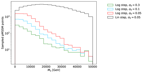
Figure 1: Distribution of the gluino mass parameter $M_{3}$ for different stepping configurations. The black distribution corresponds to Lin 0.05, which is chosen as the baseline.

The Lin 0.05 configuration results in the highest fraction of points with squark and gluino masses above 10 TeV, as seen in Table 4. Largely for this reason, the Lin 0.05 test scan is deemed the most optimal and is used as the final stepping configuration. In order to maximize the statistics of the final scan, the results of the four non-optimal test scans presented in this section are combined with the results of the final configuration. However, the contribution from these test scans is small, and the overall scan behavior follows that of Lin 0.05.

3 Selection of sampled points

Following the sampling of pMSSM points according to the procedure described in the previous section, a post-processing step is applied to further remove experimentally disfavored regions of the parameter space from the scan. A scan point is excluded if it satisfies one or more of the following criteria:

1. the LSP of the spectrum is not a neutralino,

2. the point is excluded at 95% CL by one ore more LHC Higgs searches as calculated by HiggsBounds,

3. the point is excluded at 95% CL by one or more LHC SUSY searches as calculated by SModelS 2.1[48, 49, 50, 51, 52],

4. the point is excluded at 90% CL by dark matter measurements as calculated by MicrOMEGAs 5.2.7.a, [53, 54, 55].

For item (b), boolean constraints indicating whether a point is excluded by LHC Higgs searches are computed by HiggsBounds and applied at the post-processing step. HiggsBounds tests each of the Higgs bosons individually, where in each case the potentially strongest bound is applied. A pMSSM point is rejected if it is excluded at 95% CL by at least one of the applied Higgs boson search channels. This is in addition to the inclusion of the HiggsBounds likelihood for the $H/A\rightarrow\tau\tau$ search directly in the McMC likelihood, as described in Sec. 2.1. For item (c), SModelS computes exclusion limits from LHC SMS searches for each pMSSM point by decomposing each point into all relevant SMS models, computing the cross section of the simplified model processes, and then comparing the cross section of each simplified model process to the experimental limit. The pMSSM point is rejected if any simplified model process is excluded at 95% CL. For item (d), the MicrOMEGAs package calculates exclusion limits from $Z\rightarrow$ invisible, DM direct detection experiments [55], and searches for sparticle and DM production in $e^{+}e^{-}$ collisions from LEP [54]. Points excluded by any of these measurements at 90% CL are rejected.

The DM relic density $\Omega h^{2}$ is also calculated at the post-processing step by MicrOMEGAs. Though not included in the McMC likelihood, this observable can be used to further focus on regions of the pMSSM scan that are experimentally and theoretically motivated.

An overview of the scanned pMSSM points is shown in Table 5. The first and second columns show the portions of the scan that do and do not use $\Delta a_{\mu}$ in the McMC likelihood, respectively. Note that the scan efficiency is much higher when $\Delta a_{\mu}$ is not included in the likelihood, but the fraction of points with $\Delta a_{\mu}$ near the measured value (last row) is small. The total scan statistics, corresponding to the sum of the first two columns, are shown in the final column of Table 5.

	With $\Delta a_{\mu}$	Without $\Delta a_{\mu}$	Total
Sampled points	14,194,316	16,848,695	31,043,011
McMC accepted points	156,599	6,800,642	6,957,241
Post-process accepted points	44,444	3,312,480	3,356,924
Total Efficiency	0.3%	20%	11%
Strong decoupling	5,529	577,695	583,224
$\Delta m$(LSP, gluino) $<$ 500 GeV	24	2,412	2,436
$\Delta m$(LSP, stop) $<$ 500 GeV	14	1,480	1,494
$\Delta a_{\mu}$ within measured $\pm 1\sigma$	19,540	3,212	22,752

Table 5: Summary of the scanned pMSSM points. The criteria for points with strong decoupling is that the squark, gluino masses exceed 10 TeV.

4 Results

Precision measurements of sensitive observables can be a powerful tool for constraining physics beyond the standard model. This section presents studies of how measurements of Higgs boson properties, the anomalous magnetic moment of the muon, and dark matter at current and future experiments are expected to impact the allowed pMSSM parameter space.

4.1 Higgs boson properties

Higgs boson couplings for each pMSSM point are calculated by FeynHiggs and studied in the $\kappa$-framework [56, 57], where for particle $p$ with Higgs coupling $\lambda_{p}$

$$\kappa_{p}=\frac{\lambda_{p}}{\lambda_{p,\text{SM}}}~{}.$$ (4)

The Higgs boson coupling to quarks (top, bottom, and charm) and leptons (tau and muon) are found to peak sharply the expected SM value of $\kappa=1$. This is consistent with the LHC measurements to date, which enter the McMC likelihood through the contribution from HiggsSignals. The couplings to the top quark, bottom quark, and tau lepton are shown for each pMSSM point in Figure 2. The sampled pMSSM points that are excluded in the post-processing step described in Sec. 3 are shown separately from the final accepted sample. Points accepted by the McMC but excluded at 95% CL by HiggsBounds (LHC Higgs searches) are shown in purple. Of the remaining points, those excluded at 95% CL by SModelS (LHC SUSY searches) are shown in dark blue. And of the remaining points, those excluded at 90% CL by MicrOMEGAs (DM measurements) are shown in light blue. The green distribution shows the points that are fully accepted after all post-processing steps. The distributions of $\kappa_{c}$ and $\kappa_{\mu}$ (not shown) closely resemble those of $\kappa_{t}$ and $\kappa_{\tau}$, respectively.

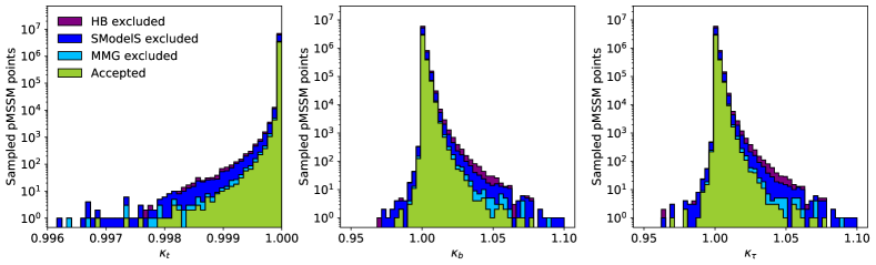
(a)

Figure 2: Higgs couplings with top quark ($\kappa_{t}$), bottom quark ($\kappa_{b}$), and tau ($\kappa_{\tau}$) calculated by FeynHiggs for each pMSSM point. Points accepted by the McMC but excluded by HiggsBounds (LHC Higgs searches) are shown in purple. Of the remaining points, those excluded by SModelS (LHC SUSY searches) are shown in dark blue. And of the remaining points, those excluded by MicrOMEGAs (DM measurements) are shown in light blue. The green distribution shows the points that are fully accepted after all post-processing steps.

The distributions found for $\kappa_{t}$, $\kappa_{b}$, and $\kappa_{\tau}$ are consistent with deviations expected for tree-level contributions from the MSSM Higgs sector (a type-II two-Higgs-doublet model) rather than genuine SUSY loop contributions to the various Higgs couplings. This observation is consistent with previous studies including Ref. [58]. The deviations from unity scale with $\sin(\beta-\alpha)+\cos(\beta-\alpha)/\tan\beta$ for $\kappa_{t}$ and with $\sin(\beta-\alpha)-\cos(\beta-\alpha)\tan\beta$ for $\kappa_{b,\tau}$ ($\alpha$ is the angle that diagonalizes the CP-even Higgs sector). For $M_{A}\to\infty$, one finds $\beta-\alpha\to\pi/2$ and $\sin(\beta-\alpha)\to 1$. Consequently, for $\tan\beta>1$ (as in this scan) one finds smaller deviations from unity for $\kappa_{t}$ and larger opposite sign deviations for $\kappa_{b,\tau}$. The pseudoscalar component of each Higgs-fermion coupling is also calculated, but is not found to deviate from zero in any of the sampled pMSSM points. Taking into account the size of the deviations of $\kappa_{t,b,\tau}$ from unity and the expected experimental precision at current and future experiments in the various $\kappa$ determinations, $\kappa_{b}$ is expected to provide most sensitivity to deviations from the SM.

Figure 3 shows the fraction of the sampled pMSSM points in the $M_{A}$–$\tan\beta$ plane having $\kappa_{b}$ within $\pm 1\%$ of unity (on the left), which roughly corresponds to the 95% CL precision expected for the combination of FCC-ee/eh/hh [59], and within $\pm 0.2\%$ of unity (on the right). The gray region is excluded by current searches for heavy MSSM Higgs bosons. The $1\%$ limit cuts away most points below $M_{A}\leq 1500$ GeV, setting an indirect lower bound on the MSSM heavy Higgs mass scale. A stronger bound can be found for the increased precision of $0.2\%$, where $M_{A}$ less than $\sim 3$ TeV would only be allowed in a small fraction of models, all with large $\tan\beta$ values. The projected limits from direct searches for heavy MSSM Higgs bosons at the HL-LHC (cyan) and the FCC-hh (green) are overlaid. Even with the full precision on $\kappa_{b}$ expected at the FCC-hh, the indirect limit is far less powerful than direct searches.

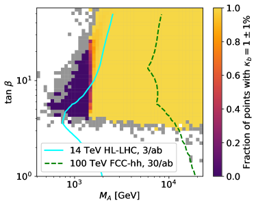
(a)

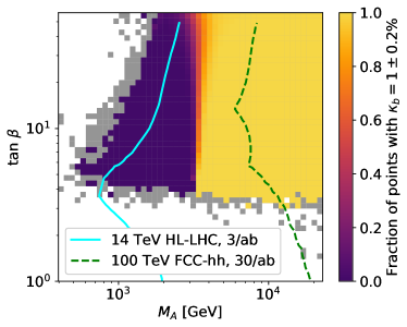
(b)

Figure 3: Fraction sampled pMSSM points with $\kappa_{b}$ within $\pm 1\%$ (left) and $\pm 0.2\%$ (right) of the SM expectation, shown as a function of $\tan\beta$ and $M_{A}$. The $\pm 1\%$ range roughly corresponds to the 95% CL precision expected for the combination of FCC-ee/eh/hh [59]. The projected limits from direct searches for heavy MSSM Higgs bosons at the HL-LHC (cyan) and the FCC-hh (green) are overlaid.

4.2 Anomalous magnetic moment of the muon

Recent measurements of the anomalous muon magnetic moment $\Delta a_{\mu}$ [47] that disagree with established SM predictions [60] at the level of 4.2 standard deviations have renewed interest in possible physics beyond the SM contributing to this observable. The McMC likelihood of the present pMSSM scan is constructed to populate the region near the measured value as well as the value predicted within the SM $(\Delta a_{\mu}=0)$. The distribution of $\Delta a_{\mu}$ for the sampled pMSSM points shown in Figure 4 exhibits the desired two-peak structure. Though much of the peak at the measured value is excluded by SModelS, approximately 10% of points passing all selection have $\Delta a_{\mu}$ within $1\sigma$ of the measurement (denoted by vertical lines).

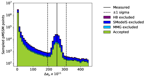
Figure 4: Distribution of $\Delta a_{\mu}$ for the sampled pMSSM points. The predicted Standard Model value corresponds to $\Delta a_{\mu}=0$, and the measured central value and uncertainties indicated by vertical lines. Points accepted by the McMC but excluded by HiggsBounds (LHC Higgs searches) are shown in purple. Of the remaining points, those excluded by SModelS (LHC SUSY searches) are shown in dark blue. And of the remaining points, those excluded by MicrOMEGAs (DM measurements) are shown in light blue. The green distribution shows the points that are fully accepted after all post-processing steps.

In order to achieve a value of $\Delta a_{\mu}$ near the measured value of $\Delta a_{\mu}=251\times 10^{-11}$, SUSY contributions involving smuon-neutralino or muon sneutrino-chargino loops are required. The corresponding particle masses should not be too high, not to suppress these loop contributions, leading typically to a light smuon (see, e.g., [61]). The fraction of sampled pMSSM points with $\Delta a_{\mu}$ within $\pm 1\sigma$ of the measured value is shown in Figure 5 as a function of the smuon mass. Three values of $\sigma$ are considered: the uncertainty on the 2021 Muon $g-2$ measurement ($59\times 10^{-11}$), the projected uncertainty at the end of running of the Muon $g-2$ experiment (a factor of two improvement in over 2021 in the combined experimental and theoretical uncertainty), and a potential future precision benchmark of five times higher precision than the 2021 result. The fraction of sampled points satisfying the $\pm 1\sigma$ criterion is high for low values of the smuon mass ($<500$ GeV).

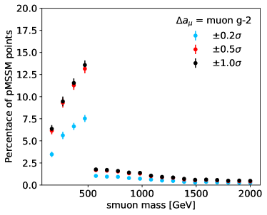
(a)

Figure 5: Fraction of scanned pMSSM points with $\Delta a_{\mu}$ within $\pm 1\sigma$ of the measured value, as a function of the smuon mass. The black line corresponds to the measured 2021 uncertainty $\sigma=59\times 10^{-11}$. The red and blue lines correspond to a reduction in the total uncertainty by a factor of two and five, respectively.

4.3 Electroweakino dark matter

For each pMSSM point in the scan, the dark matter particle is taken to be the lightest neutralino in the model, $\tilde{\chi}^{0}_{1}$. The DM relic density ($\Omega h^{2}$) and DM-nucleon cross sections are calculated by MicrOMEGAs. Figure 6 shows the fraction of pMSSM points surviving after limits from existing searches have been applied: from left to right, points are removed if they are excluded by LHC SMS searches (SModelS), BSM Higgs searches (HiggsBounds), and DM/LEP measurements (MicrOMEGAs). The three rows show the impact on different variable distributions: Figure 6 (a) shows the lightest neutralino vs. lightest chargino mass plane, (b) shows the relic density vs. DM mass, and (c) shows the spin-independent DM-neutron cross section vs. DM mass.

LHC searches for heavy stable charged particles (HSCPs) provide strong exclusions, but because HSCPs arise in the MSSM electroweakino sector primarily through small mass splittings between charged and neutral winos, these exclusions should be interpreted qualitatively rather than quantitatively.

In the left panel of Figure 6a, HSCP searches at the LHC exclude nearly all sampled points in the region near $m(\tilde{\chi}^{0}_{1})\sim m(\tilde{\chi}^{+}_{1})\in 100-1000$ GeV. The excluded region at low neutralino mass near $m(\tilde{\chi}^{+}_{1})\sim 100$ GeV, where $<10\%$ of pMSSM points survive, corresponds to the exclusion from searches for chargino pair production with $\tilde{\chi}^{\pm}_{1}\rightarrow W^{\pm}\tilde{\chi}^{0}_{1}$. The exclusion in the dark pink region from $m(\tilde{\chi}^{0}_{1})\sim 100-500$ GeV, which corresponds to 40-50% of points remaining, is dominated by searches for the following final states:

• $\tilde{\chi}^{+}_{1}\tilde{\chi}^{-}_{1}$ production with $\tilde{\chi}^{\pm}_{1}\rightarrow W^{\pm}\tilde{\chi}^{0}_{1}$;

• $\tilde{\chi}^{\pm}_{1}\tilde{\chi}^{0}_{2}$ production with $\tilde{\chi}^{\pm}_{1}\rightarrow W^{\pm}\tilde{\chi}^{0}_{1}$ and $\tilde{\chi}^{0}_{2}\rightarrow H\tilde{\chi}^{0}_{1}$;

• $\tilde{\chi}^{\pm}_{1}\tilde{\chi}^{0}_{2}$ production with $\tilde{\chi}^{\pm}_{1}\rightarrow W^{\pm}\tilde{\chi}^{0}_{1}$ and $\tilde{\chi}^{0}_{2}\rightarrow Z\tilde{\chi}^{0}_{1}$.

The right panel of Figure 6a shows the exclusions from MicrOMEGAs, which are dominated by mass limits from LEP (chargino mass $<100$ GeV) and limits from $Z\rightarrow$ invisible (chargino mass $\sim 100-300$ GeV).

Figure 6b shows the impact of existing measurements as a function of DM relic density and mass. The Planck measurement of the DM relic density [63], $\Omega h^{2}=0.120\pm 0.001$, is indicated by a horizontal line in each panel. The pMSSM scan populates values of this parameter over a very wide range compared to the experimental precision. The left panel shows the fraction of points surviving SModelS. The Z-funnel, where the Z boson contributes resonantly to the DM annihilation cross section, is clearly visible. Points with $m(\tilde{\chi}^{0}_{1})>m_{Z}$ and relic density less than $\sim 0.1$ (dark purple region) are excluded by HSCP searches. The excluded diagonal strip at $m(\chi^{0}_{1})<100$ GeV corresponds to searches for slepton pair production. The right panel shows that points with DM mass near $m_{Z}/2$ and relic density less than $\sim 0.1$ are excluded by MicrOMEGAS (specifically, DM direct detection experients and mass limits from LEP). Points with DM mass less than $\sim 1$ GeV are excluded by limits from $Z\rightarrow$ invisible for for lower relic densities.

Finally, Figure 6c shows exclusions in terms of the DM candidate mass and the spin-independent DM-neutron cross section (the DM-proton cross section yields a similar distribution). Few points are sampled with DM mass below 1 GeV: this corresponds to the lower limit on $M_{1}$ used in the scan, and points with lower neutralino masses require some mixing between bino and other electroweakino states. In the left panel, LHC HSCP searches exclude points with high cross section, with the strongest limits in the range 100-1000 GeV. In the right panel, the exclusion due to DM direct detection experiments is clearly visible at high cross section values in the region above $m(\chi_{1}^{0})\sim 10$ GeV.

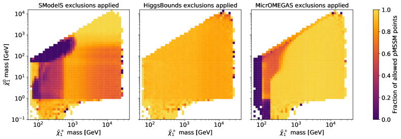
(a) Mass of neutralino vs. chargino

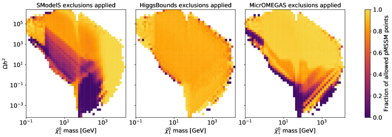
(b) DM relic density vs. neutralino mass

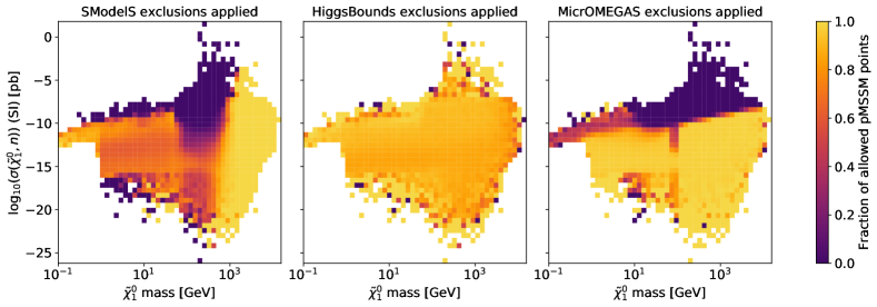
(c) Spin-independent neutralino-neutron cross section vs. neutralino mass

Figure 6: Fraction of sampled pMSSM points after applying limits from existing measurements: from left to right, LHC SMS searches (SModelS), BSM Higgs searches (HiggsBounds), and DM/LEP measurements (MicrOMEGAs). Shown as a function of (a) neutralino vs. chargino mass, (b) relic density vs. neutralino mass, and (c) the spin-independent neutralino-neutron cross section vs. neutralino mass. The Planck measurement of $\Omega h^{2}$ is shown as a black line in (b).

The DM candidate particle is a superposition of electroweakino states (bino, wino, and higgsino). Each pMSSM point is labelled by the electroweakino comprising the largest component of $\tilde{\chi}^{0}_{1}$, thereby separating the scan into samples with bino-, wino-, and higgsino-like DM. Table 6 shows the breakdown of pMSSM points by the composition of the DM candidate. The two-dimensional distribution of the DM candidate mass and relic density is shown for each component sample in Figure 7. The sampled points with very high relic density are dominated by models with bino-like DM. Wino-like DM, on the other hand, is concentrated at low values of $\Omega h^{2}$. Near the measured value of the relic density, wino-, bino-, and higgsino-like DM all contribute. Points that are excluded by SModelS, HiggsBounds, and MicrOMEGAS are shown in light gray.

	McMC accepted	Post-process accepted
Mostly wino	872,256	188,576
Mostly bino	5,513,680	3,071,103
Mostly higgsino	506,469	97,222
Mixed wino/bino	172	6
Mixed bino/higgsino	9,219	2
Mixed wino/higgsino	8,100	1
Other	47,445	14

Table 6: Number of scanned pMSSM points with different composition of the DM candidate. The DM candidate is considered mostly pure if a single electroweakino comprises $>80\%$ of the admixture and mixed if two components each contribute $>40\%$.

Figure 7: Distribution of sampled pMSSM points as function of the DM relic density vs. DM candidate mass. Points excluded by existing measurements (as implemented in SModelS, HiggsBounds, and MicrOMEGAS) are shown in light gray. The remaining points are broken down by the electroweakino composition of the DM candidate. The DM candidate is considered mostly pure if a single electroweakino comprises $>80\%$ of the admixture, and mixed otherwise.

Figure 8a shows the distribution of neutralino vs. chargino mass, with each point color-coded according to the DM composition. In the left panel, points excluded by SModelS, HiggsBounds, and MicrOMEGAS are shown in light gray, as in Figure 7. Because wino- and bino-like dark matter tend to have compressed spectra, where $m(\tilde{\chi}^{0}_{1})\sim m(\tilde{\chi}^{+}_{1})$, these points are clustered on the diagonal. The right panel shows the same distribution, but with the additional criterion that points with $\Omega h^{2}$ differing from the Planck measurement by more than 50% are also colored gray.

Figure 8b shows the distribution of the DM candidate mass and DM-neutron spin-independent cross section broken down by the DM composition. The colored points in the left panel correspond to models that are not excluded by existing measurements (SModelS, HiggsBounds, and MicrOMEGAS), while in the right panel the colored points are further required to be within 50% of the measured relic density.

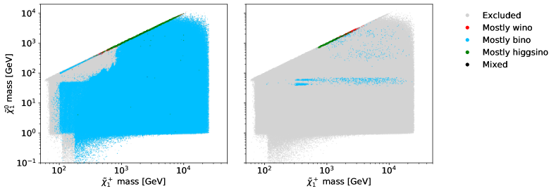
(a)

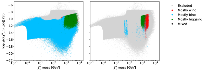
(b)

Figure 8: Distribution of (a) the chargino and neutralino mass, and (b) the DM candidate mass and DM-neutron spin-independent cross section for the sampled pMSSM points. In the left panels, points excluded by existing measurements (as implemented in SModelS, HiggsBounds, and MicrOMEGAS) are shown in light gray. The remaining points are broken down by the electroweakino composition of the DM candidate. The right panels show the same distribution with the additional criterion that points with $\Omega h^{2}$ differing from the Planck measurement by more than 50% are also colored gray.

The requirement that models yield a DM relic density within 50% of the Planck measurement rules out all sampled points with DM mass less than $\sim 25$ GeV (dominantly bino-like). The surviving points include wino, bino, or higgsino dark matter candidates.

5 Conclusion

An extensive scan of the pMSSM parameter space has been completed for Snowmass 2021. The scanned parameter space covers ranges that will be accessible ranges to many future collider scenarios, including electron, muon, and hadron colliders at a center of mass energies up to 100 TeV. The choice of a Markov chain Monte Carlo sampling method ensures that the 19 dimensional parameter space is explored efficiently. The inclusion of current measurements in the likelihood ensures that space that is experimentally disfavored is not prioritized. Additional selection at the post-processing stage accounts for the effects of LHC Higgs measurements, LHC searches for SUSY and other new phenomena, and DM measurements. The impact of future precision measurements on Higgs couplings, $\Delta a_{\mu}$, and DM quantities is presented.

The next steps for this ongoing Snowmass pMSSM effort include performing studies with simulated events in order to quantitatively assess the sensitivity of selected future colliders in the context of the pMSSM. Studies will be based on common tools, such as Pythia8 for event generation and Delphes3 for detector simulation, and will employ implementations of recent searches for BSM physics at the LHC with optimization for future colliders. Following these studies, pMSSM points not excluded by current or future experiments can be used to identify promising new regions in the space of experimental observables (e.g. particle momenta and invariant masses) in order to guide design of future analyses and detectors. We are exploring the use of machine-learning-based clustering techniques based on $k$-means [64] and density-based clustering [65] to identify categories and group pMSSM models with similar experimental signatures together.

Appendix A Coverage of the scan

Throughout this section, sampled pMSSM points that are excluded at post-processing are shown separately from the final accepted sample. Points accepted by the McMC but excluded at 95% CL by HiggsBounds (LHC Higgs searches) are shown in purple. Of the remaining points, those excluded at 95% CL by SModels (LHC SUSY searches) are shown in dark blue. And of the remaining points, those excluded at 90% CL by MicrOMEGAs (dark matter measurements) are shown in light blue. The green distribution shows the points that are fully accepted after all post-processing steps.

A.1 pMSSM parameters

The distribution of the sampled trilinear couplings ($A_{t}$, $A_{b}$, and $A_{l}$) are shown in Figure 9. The symmetry across 0 shows that the random selection of initial scan points does indeed populate all sign combinations effectively.

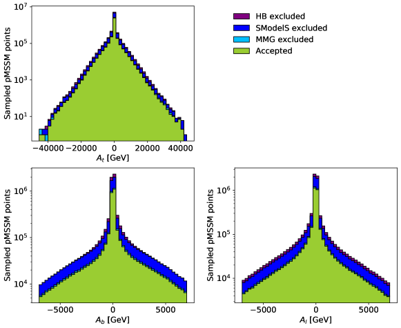
Figure 9: Distribution of the trilinear couplings $A_{t}$, $A_{b}$, and $A_{l}$ of sampled pMSSM points.

The distributions of the sampled gaugino mass parameters ($\mu$, $M_{1}$, $M_{2}$, and $M_{3}$) are shown in Figure 10. Again, good symmetry across 0 is observed in $\mu$, $M_{1}$, and $M_{2}$. The power of LHC SUSY searches is visible at low values of these mass parameters, where the SModelS exclusion rules out the majority of points accepted by the McMC.

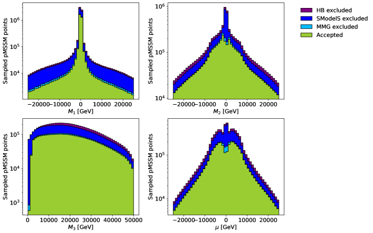
Figure 10: Distribution of the gaugino mass parameters $M_{1}$, $M_{2}$, $M_{3}$, and $\mu$ of sampled pMSSM points.

The sampled values of slepton mass parameters are shown in Figure 11 for left-handed (left) and right-handed (right) sleptons. The peak at low values of the smuon/selectron mass corresponds to those points with large $\Delta a_{\mu}$. These are largely excluded by SModelS.

Figure 11: Distribution of slepton mass parameters $m_{\tilde{L}^{1,2}}$, $m_{\tilde{L}^{3}}$, $m_{\tilde{R}^{1,2}}$, and $m_{\tilde{R}^{3}}$ of sampled pMSSM points.

The sampled squark mass parameters are shown in Figure 12: the left column shows the right-handed up-type, the center column shows the right-handed down-type, and the right column shows the left-handed squark masses. Again, LHC searches have been able to exclude much of the parameter space at low squark masses, as showwn by the SModelS exclusion.

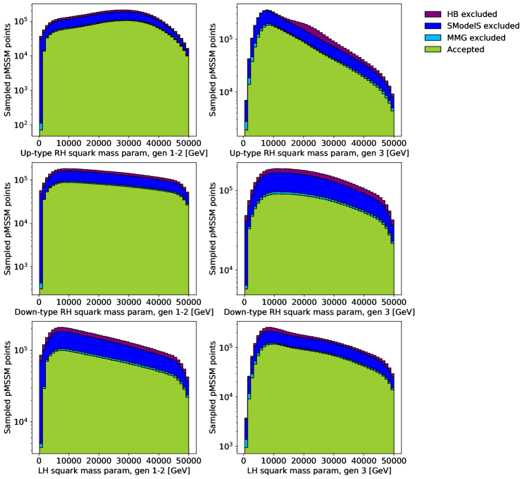
Figure 12: Distribution of squark mass parameters (top) $m_{\tilde{u}^{1,2}}$, $m_{\tilde{u}^{3}}$, (middle) $m_{\tilde{d}^{1,2}}$, $m_{\tilde{d}^{3}}$, (bottom) $m_{\tilde{q}^{1,2}}$, $m_{\tilde{q}^{3}}$ of sampled pMSSM points.

The pMSSM Higgs paramters, the mass of the heavy Higgs boson $M_{A}$ and $\tan\beta$, are shown in Figure 13. HiggsBounds, which includes dedicated LHC searches for the decay of the heavy Higgs, and SModelS exclude all points with $M_{A}<500$ GeV.

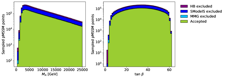
Figure 13: The sampled mass of the heavy Higgs boson $M_{A}$ (left), and $\tan\beta$ (right) for the sampled pMSSM points.

A.2 Sparticle masses

This section shows the distributions of sparticle masses of the sampled pMSSM points. Figure 14 shows the slepton masses, and Figure 15 shows the sneutrino masses. Figure 16 shows the sbottom and stop quark masses, and Figure 17 shows the gluino mass. The neutralino and chargino masses are shown in Figures 18 and 19, respectively.

Figure 14: Slepton masses

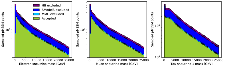
Figure 15: Sneutrino masses

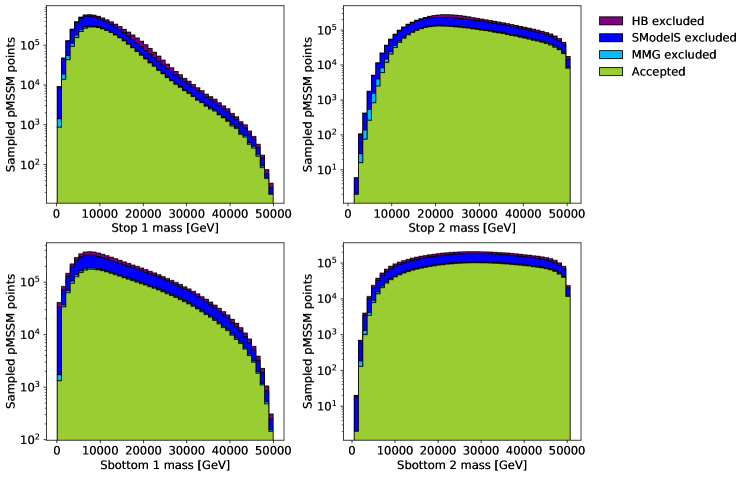
Figure 16: Heavy squark masses

Figure 17: Gluino mass

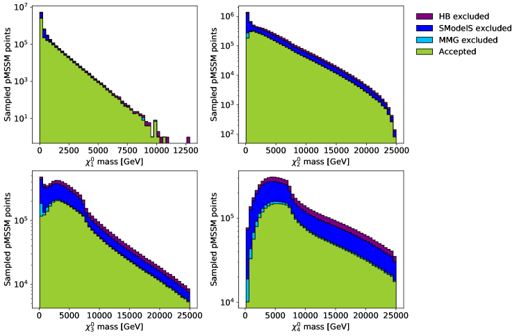
Figure 18: Neutralino masses

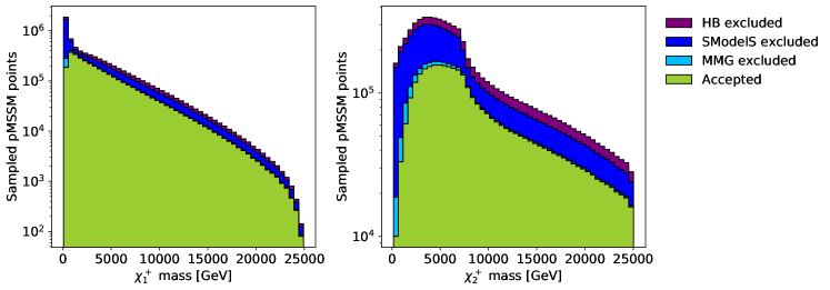
Figure 19: Chargino masses

A.3 Standard model observables

The top and bottom quark masses, along with the strong coupling constant $\alpha_{S}$, for each pMSSM point are shown in Figure 20.

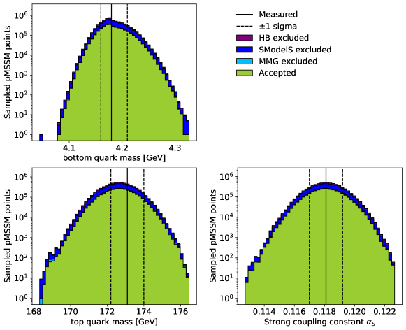
Figure 20: The bottom quark mass, top quark mass, and strong coupling constant for each sampled pMSSM point, with the measured value and uncertainties indicated by vertical lines.

References

- [1] P. Fayet “Supersymmetry and weak, electromagnetic and strong interactions” In Physics Letters B 64.2, 1976, pp. 159–162 DOI: https://doi.org/10.1016/0370-2693(76)90319-1
- [2] P. Fayet “Spontaneously broken supersymmetric theories of weak, electromagnetic and strong interactions” In Physics Letters B 69.4, 1977, pp. 489–494 DOI: https://doi.org/10.1016/0370-2693(77)90852-8
- [3] Glennys R. Farrar and Pierre Fayet “Phenomenology of the production, decay, and detection of new hadronic states associated with supersymmetry” In Physics Letters B 76.5, 1978, pp. 575–579 DOI: https://doi.org/10.1016/0370-2693(78)90858-4
- [4] Pierre Fayet “Relations between the masses of the superpartners of leptons and quarks, the goldstino coupling and the neutral currents” In Physics Letters B 84.4, 1979, pp. 416–420 DOI: https://doi.org/10.1016/0370-2693(79)91229-2
- [5] Savas Dimopoulos and Howard Georgi “Softly broken supersymmetry and SU(5)” In Nuclear Physics B 193.1, 1981, pp. 150–162 DOI: https://doi.org/10.1016/0550-3213(81)90522-8
- [6] Ali H. Chamseddine, Richard L. Arnowitt and Pran Nath “Locally Supersymmetric Grand Unification” In Phys. Rev. Lett. 49, 1982, pp. 970 DOI: 10.1103/PhysRevLett.49.970
- [7] Riccardo Barbieri, S. Ferrara and Carlos A. Savoy “Gauge Models with Spontaneously Broken Local Supersymmetry” In Phys. Lett. B 119, 1982, pp. 343 DOI: 10.1016/0370-2693(82)90685-2
- [8] Luis E. Ibanez “Locally Supersymmetric SU(5) Grand Unification” In Phys. Lett. B 118, 1982, pp. 73–78 DOI: 10.1016/0370-2693(82)90604-9
- [9] Lawrence J. Hall, Joseph D. Lykken and Steven Weinberg “Supergravity as the Messenger of Supersymmetry Breaking” In Phys. Rev. D 27, 1983, pp. 2359–2378 DOI: 10.1103/PhysRevD.27.2359
- [10] Johan Alwall, Philip C. Schuster and Natalia Toro “Simplified models for a first characterization of new physics at the LHC” In Physical Review D 79.7 American Physical Society (APS), 2009 DOI: 10.1103/physrevd.79.075020
- [11] Daniele Alves et al. “Simplified models for LHC new physics searches” In Journal of Physics G: Nuclear and Particle Physics 39.10 IOP Publishing, 2012, pp. 105005 DOI: 10.1088/0954-3899/39/10/105005
- [12] S. Chatrchyan et al. “Interpretation of searches for supersymmetry with simplified models” In Physical Review D 88.5 American Physical Society (APS), 2013 DOI: 10.1103/physrevd.88.052017
- [13] ATLAS Collaboration “Summary of the ATLAS experiment’s sensitivity to supersymmetry after LHC Run 1 — interpreted in the phenomenological MSSM” In JHEP 2015.10 Springer ScienceBusiness Media LLC, 2015 DOI: 10.1007/jhep10(2015)134
- [14] CMS Collaboration “Phenomenological MSSM interpretation of CMS searches in pp collisions at and 8 TeV” In JHEP 2016.10 Springer ScienceBusiness Media LLC, 2016 DOI: 10.1007/jhep10(2016)129
- [15] G. Aad et al. “Summary of the ATLAS experiment’s sensitivity to supersymmetry after LHC Run 1 — interpreted in the phenomenological MSSM” In Journal of High Energy Physics 2015.10 Springer ScienceBusiness Media LLC, 2015 DOI: 10.1007/jhep10(2015)134
- [16] V. Khachatryan et al. “Phenomenological MSSM interpretation of CMS searches in pp collisions at and 8 TeV” In Journal of High Energy Physics 2016.10 Springer ScienceBusiness Media LLC, 2016 DOI: 10.1007/jhep10(2016)129
- [17] Carola F Berger, James S Gainer, JoAnne L Hewett and Thomas G Rizzo “Supersymmetry without prejudice” In Journal of High Energy Physics 2009.02 Springer ScienceBusiness Media LLC, 2009, pp. 023–023 DOI: 10.1088/1126-6708/2009/02/023
- [18] Matthew W. Cahill-Rowley et al. “The new look pMSSM with neutralino and gravitino LSPs” In The European Physical Journal C 72.9 Springer ScienceBusiness Media LLC, 2012 DOI: 10.1140/epjc/s10052-012-2156-1
- [19] Federico Ambrogi et al. “On the coverage of the pMSSM by simplified model results” In The European Physical Journal C 78.3 Springer ScienceBusiness Media LLC, 2018 DOI: 10.1140/epjc/s10052-018-5660-0
- [20] S. S. AbdusSalam “Benchmark Models, Planes, Lines and Points for Future SUSY Searches at the LHC” In Eur. Phys. J. C 71, 2011, pp. 1835 DOI: 10.1140/epjc/s10052-011-1835-7
- [21] W. Porod “SPheno, a program for calculating supersymmetric spectra, SUSY particle decays and SUSY particle production at e+e- colliders” In Computer Physics Communications 153.2, 2003, pp. 275–315 DOI: https://doi.org/10.1016/S0010-4655(03)00222-4
- [22] W. Porod and F. Staub “SPheno 3.1: extensions including flavour, CP-phases and models beyond the MSSM” In Computer Physics Communications 183.11 Elsevier BV, 2012, pp. 2458–2469 DOI: 10.1016/j.cpc.2012.05.021
- [23] P Skands et al. “SUSY Les Houches Accord: Interfacing SUSY Spectrum Calculators, Decay Packages, and Event Generators” In Journal of High Energy Physics 2004.07 Springer ScienceBusiness Media LLC, 2004, pp. 036–036 DOI: 10.1088/1126-6708/2004/07/036
- [24] Anthony O’Hagan and Jonathan J. Forster “Kendall’s Advanced Theory of Statistics, volume 2B: Bayesian Inference” London: Arnold, 1994
- [25] A. A. Markov “Extension of the limit theorems of probability theory to a sum of variables connected in a chain” reprinted in Appendix B of: R. Howard, Dynamic Probabilistic Systems, volume 1: Markov Chains John WileySons, 1971
- [26] N. Metropolis al. “Equation of state calculations by fast computing machines” In J. Chem. Phys 21 1087, 1953 DOI: 10.1063/1.1699114
- [27] W. K. Hastings “Monte Carlo sampling methods using Markov chains and their applications” In Biometrika 12.97, 1970 DOI: 10.1093/biomet/57.1.97
- [28] B. A. Berg “Markov chain Monte Carlo simulations and their statistical analysis” Singapore: World Scientific, 2004
- [29] Henning Bahl et al. “Precision calculations in the MSSM Higgs-boson sector with FeynHiggs 2.14”, 2019 arXiv:1811.09073 [hep-ph]
- [30] Henning Bahl, Sven Heinemeyer, Wolfgang Hollik and Georg Weiglein “Reconciling EFT and hybrid calculations of the light MSSM Higgs-boson mass” In The European Physical Journal C 78.1 Springer ScienceBusiness Media LLC, 2018 DOI: 10.1140/epjc/s10052-018-5544-3
- [31] Henning Bahl and Wolfgang Hollik “Precise prediction for the light MSSM Higgs-boson mass combining effective field theory and fixed-order calculations” In The European Physical Journal C 76.9 Springer ScienceBusiness Media LLC, 2016 DOI: 10.1140/epjc/s10052-016-4354-8
- [32] T. Hahn et al. “High-Precision Predictions for the LightCP-Even Higgs Boson Mass of the Minimal Supersymmetric Standard Model” In Physical Review Letters 112.14 American Physical Society (APS), 2014 DOI: 10.1103/physrevlett.112.141801
- [33] Markus Frank et al. “The Higgs boson masses and mixings of the complex MSSM in the Feynman-diagrammatic approach” In Journal of High Energy Physics 2007.02 Springer ScienceBusiness Media LLC, 2007, pp. 047–047 DOI: 10.1088/1126-6708/2007/02/047
- [34] G. Degrassi et al. “Towards high-precision predictions for the MSSM Higgs sector” In The European Physical Journal C 28.1 Springer ScienceBusiness Media LLC, 2003, pp. 133–143 DOI: 10.1140/epjc/s2003-01152-2
- [35] S. Heinemeyer, W. Hollik and G. Weiglein “The masses of the neutral -even Higgs bosons in the MSSM: Accurate analysis at the two-loop level” In The European Physical Journal C 9.2 Springer ScienceBusiness Media LLC, 1999, pp. 343–366 DOI: 10.1007/s100529900006
- [36] S. Heinemeyer, W. Hollik and G. Weiglein “FeynHiggs: a program for the calculation of the masses of the neutral -even Higgs bosons in the MSSM” In Computer Physics Communications 124.1 Elsevier BV, 2000, pp. 76–89 DOI: 10.1016/s0010-4655(99)00364-1
- [37] F. Mahmoudi “SuperIso v2.3: A program for calculating flavor physics observables in supersymmetry” In Computer Physics Communications 180.9 Elsevier BV, 2009, pp. 1579–1613 DOI: 10.1016/j.cpc.2009.02.017
- [38] Philip Bechtle et al. “HiggsSignals: Confronting arbitrary Higgs sectors with measurements at the Tevatron and the LHC” In The European Physical Journal C 74.2 Springer ScienceBusiness Media LLC, 2014 DOI: 10.1140/epjc/s10052-013-2711-4
- [39] Philip Bechtle et al. “HiggsSignals-2: Probing new physics with precision Higgs measurements in the LHC 13 TeV era” In Eur. Phys. J. C 81.2, 2021, pp. 145 DOI: 10.1140/epjc/s10052-021-08942-y
- [40] P. Bechtle et al. “HiggsBounds: Confronting arbitrary Higgs sectors with exclusion bounds from LEP and the Tevatron” In Computer Physics Communications 181.1 Elsevier BV, 2010, pp. 138–167 DOI: 10.1016/j.cpc.2009.09.003
- [41] Philip Bechtle et al. “Recent Developments in HiggsBounds and a Preview of HiggsSignals”, 2013 arXiv:1301.2345 [hep-ph]
- [42] Philip Bechtle et al. “HiggsBounds-4: improved tests of extended Higgs sectors against exclusion bounds from LEP, the Tevatron and the LHC” In The European Physical Journal C 74.3 Springer ScienceBusiness Media LLC, 2014 DOI: 10.1140/epjc/s10052-013-2693-2
- [43] Philip Bechtle et al. “Applying exclusion likelihoods from LHC searches to extended Higgs sectors” In The European Physical Journal C 75.9 Springer ScienceBusiness Media LLC, 2015 DOI: 10.1140/epjc/s10052-015-3650-z
- [44] Philip Bechtle et al. “HiggsBounds-5: Testing Higgs Sectors in the LHC 13 TeV Era” In Eur. Phys. J. C 80.12, 2020, pp. 1211 DOI: 10.1140/epjc/s10052-020-08557-9
- [45] Peter Athron et al. “GM2Calc: precise MSSM prediction for of the muon” In The European Physical Journal C 76.2 Springer ScienceBusiness Media LLC, 2016 DOI: 10.1140/epjc/s10052-015-3870-2
- [46] Peter Athron et al. “Two-loop Prediction of the Anomalous Magnetic Moment of the Muon in the Two-Higgs Doublet Model with GM2Calc 2”, 2021 arXiv:2110.13238 [hep-ph]
- [47] B. Abi et al. “Measurement of the Positive Muon Anomalous Magnetic Moment to 0.46 ppm” In Physical Review Letters 126.14 American Physical Society (APS), 2021 DOI: 10.1103/physrevlett.126.141801
- [48] Sabine Kraml et al. “SModelS: a tool for interpreting simplified-model results from the LHC and its application to supersymmetry” In Eur. Phys. J. C 74, 2014, pp. 2868 DOI: 10.1140/epjc/s10052-014-2868-5
- [49] Federico Ambrogi et al. “SModelS v1.1 user manual: Improving simplified model constraints with efficiency maps” In Comput. Phys. Commun. 227, 2018, pp. 72–98 DOI: 10.1016/j.cpc.2018.02.007
- [50] Federico Ambrogi “SModelS v1.2: long-lived particles, combination of signal regions, and other novelties” In Comput. Phys. Commun. 251, 2020, pp. 106848 DOI: 10.1016/j.cpc.2019.07.013
- [51] Gaël Alguero et al. “New developments in SModelS” In PoS TOOLS2020, 2021, pp. 022 DOI: 10.22323/1.392.0022
- [52] Gaël Alguero et al. “Constraining new physics with SModelS version 2” arXiv, 2021 DOI: 10.48550/ARXIV.2112.00769
- [53] G. Bélanger, F. Boudjema, A. Pukhov and A. Semenov “micrOMEGAs 3: A program for calculating dark matter observables” In Computer Physics Communications 185.3 Elsevier BV, 2014, pp. 960–985 DOI: 10.1016/j.cpc.2013.10.016
- [54] D. Barducci et al. “Collider limits on new physics within micrOMEGAs 4.3”, 2017 arXiv:1606.03834 [hep-ph]
- [55] G. Bélanger, F. Boudjema, A. Pukhov and A. Semenov “Dark matter direct detection rate in a generic model with micrOMEGAs 2.2” In Computer Physics Communications 180.5 Elsevier BV, 2009, pp. 747–767 DOI: 10.1016/j.cpc.2008.11.019
- [56] LHC Higgs Cross Section Working Group et al. “LHC HXSWG interim recommendations to explore the coupling structure of a Higgs-like particle” arXiv, 2012 DOI: 10.48550/ARXIV.1209.0040
- [57] C T Potter et al. “Handbook of LHC Higgs Cross Sections: 3. Higgs Properties: Report of the LHC Higgs Cross Section Working Group” CERN, 2013 DOI: 10.5170/CERN-2013-004
- [58] H. Bahl et al. “HL-LHC and ILC sensitivities in the hunt for heavy Higgs bosons” In Eur. Phys. J. C 80.10, 2020, pp. 916 DOI: 10.1140/epjc/s10052-020-08472-z
- [59] J. Blas et al. “Higgs Boson studies at future particle colliders” In Journal of High Energy Physics 2020.1 Springer ScienceBusiness Media LLC, 2020 DOI: 10.1007/jhep01(2020)139
- [60] T. Aoyama “The anomalous magnetic moment of the muon in the Standard Model” In Phys. Rept. 887, 2020, pp. 1–166 DOI: 10.1016/j.physrep.2020.07.006
- [61] Manimala Chakraborti, Sven Heinemeyer and Ipsita Saha “The new “MUON G-2” result and supersymmetry” In Eur. Phys. J. C 81.12, 2021, pp. 1114 DOI: 10.1140/epjc/s10052-021-09900-4
- [62] Manimala Chakraborti, Sven Heinemeyer and Ipsita Saha “Improved measurements and wino/higgsino dark matter” In Eur. Phys. J. C 81.12, 2021, pp. 1069 DOI: 10.1140/epjc/s10052-021-09814-1
- [63] Planck Collaboration: N. Aghanim al. “Planck 2018 results” In Astronomy & Astrophysics 641 EDP Sciences, 2020, pp. A6 DOI: 10.1051/0004-6361/201833910
- [64] S. Lloyd “Least squares quantization in PCM” In IEEE Trans. Inf. Theory 28.2, 1982, pp. 129–137 DOI: 10.1109/TIT.1982.1056489
- [65] Martin Ester, Hans-Peter Kriegel, Jörg Sander and Xiaowei Xu “A Density-Based Algorithm for Discovering Clusters in Large Spatial Databases with Noise” In Proceedings of the Second International Conference on Knowledge Discovery and Data Mining, KDD’96 Portland, Oregon: AAAI Press, 1996, pp. 226–231