Open Set Classification of Untranscribed Handwritten Documents

Abstract

Huge amounts of digital page images of important manuscripts are preserved in archives worldwide. The amounts are so large that it is generally unfeasible for archivists to adequately tag most of the documents with the required metadata so as to allow proper organization of the archives and effective exploration by scholars and the general public. The class or “typology” of a document is perhaps the most important tag to be included in the metadata. The technical problem is one of automatic classification of documents, each consisting of a set of untranscribed handwritten text images, by the textual contents of the images. The approach considered is based on “probabilistic indexing”, a relatively novel technology which allows to effectively represent the intrinsic word-level uncertainty exhibited by handwritten text images. We assess the performance of this approach on a large collection of complex notarial manuscripts from the Spanish Archivo Hostórico Provincial de Cádiz, with promising results.

1 Introduction

Content-based classification of manuscripts is an important task that is generally performed by expert archivists. Unfortunately, however, many manuscript collections are so vast that it is not possible to have the huge number of archive experts that would be needed to perform this task.

Current approaches for textual-content-based manuscript classification require the handwritten images to be first transcribed into text – but achieving sufficiently accurate transcripts are generally unfeasible for large sets of historical manuscripts. We propose a new approach to perform automatically this classification task which does not rely on any explicit image transcripts.

Hereafter, bundles or folders of manuscript images are called “image bundles” or just “bundles” or “books”. A bundle may contain several “files”, also called “acts” or just “image documents”. The task consists of classifying a given image document, that may range from a few to tens of handwritten text images, into a predefined set of classes or “types”. Classes are associated with the topic or (semantic) content conveyed by the text written in the images of the document.

This task is different from other related tasks which, are often called with similar names, such as “content-based image classification”, applied to single, natural scene (not text) images, and “image document classification”, where classification is based on visual appearance or page layout. See [12] for a more detailed discussion on these differences, as well as references to previous publications dealing with related problems, but mainly aimed at printed text.

Our task is comparable to the time-honoured and well known task of content-based document classification, were the data are plain text documents. Popular examples of this traditional task, are Twenty News Groups, Reuters, WebKB, etc. [11, 9, 1]. The task here considered (textual-content-based handwritten text image document classification), is similar, except for a severe difference: our data are sets of digital images of handwritten text rather than flile of (electronic) plain text. The currently accepted wisdom to approach our task would be to split the process into two sequential stages. First, a handwritten text recognition (HTR) system is used to transcribe the images into text and, second, content-based document classification methods, such as those referred to above, can be applied to the resulting text documents.

This approach might work to some extent for simple manuscripts, where HTR can provide over 90% word recognition accuracy [17]. But it is not an option for large historical collections, where the best available HTR systems can only provide word recognition accuracies as low as 40-60% [17, 14, 4]. This is the case of the collection which motivates this work, which encompasses millions of handwritten notarial files from the Spanish Archivo Histórico Provincial de Cádiz. A small subset of these manuscripts was considered in the Carabela project [4] and the average word recognition accuracy achieved was below 65% [14], dropping to 46% or less when conditions are closer to real-world usage [4]. Clearly, for these kinds of manuscript collections, the aforementioned two-stage idea would not work and more holistic approaches are needed.

In previous works [4, 12], we have proposed an approach which strongly relies on the so-called probabilistic indexing (PrIx) technology, recently developed to deal with the intrinsic word-level uncertainty generally exhibited by handwritten text and, more so, by historical handwritten text images [20, 3, 10, 13, 19]. This technology was primarily developed to allow search and retrieval of textual information in large untranscribed manuscript collections [3, 18, 4].

In our proposal, PrIx provides the probability distribution of words which are likely written in the images, from which statistical expectations of word and document frequencies are estimated. These estimates are then used to compute well-known text features such as Information Gain and $\operatorname*{\operatorname*{Tf}\!\cdot\!\operatorname*{Idf}}$ [11], which are in turn considered inputs to a Multilayer Perceptron classifier [12].

In this paper, we further develop and consolidate this approach and, as mentioned above, apply it to a new collection of handwritten notarial documents from the Archivo Provincial de Cádiz. In contrast with [4, 12], where the underlying class structure was very limited (just three rather artificial classes), here the classes correspond to real typologies, such as power of attorney, lease, will, etc. Our results clearly show the capabilities of the proposed approach, which achieves classification accuracy as high as 90–97%, depending on the specific set of manuscripts considered.

2 Probabilistic Indexing of Handwritten Text Images

The Probabilistic Indexing (PrIx) framework was proposed to deal with the intrinsic word-level uncertainty generally exhibited by handwritten text in images and, in particular, images of historical manuscripts. It draws from ideas and concepts previously developed for keyword spotting, both in speech signals and text images. However, rather than caring for ”key” words, any element in an image which is likely enough to be interpreted as a word is detected and stored, along with its relevance probability (RP) and its location in the image. These text elements are referred to as “pseudo-word spots”.

Following [20, 13], the image-region word RP is denoted as $P(R\!=\!1\mid X\!=\!x,V\!=v\!)$, but for the sake of conciseness, the random variable names will be omitted and, for $R=1$, we will simply write $R$. As discussed in [21], this RP can be simply approximated as:

$$P(R\mid x,v)=\sum_{b\sqsubseteq x}P(R,b\mid x,v)\approx\max_{b\sqsubseteq x}P(v\mid x,b)$$ (1)

where $b$ is a small, word-sized image sub-region or Bounding Box (BB), and with $b\sqsubseteq x$ we mean the set of all BBs contained in $x$. $P(v\mid x,b)$ is just the posterior probability needed to “recognize” the BB image $(x,b)$. Therefore, assuming the computational complexity entailed by (1) is algorithmically managed, any sufficiently accurate isolated word classifier can be used to obtain $P(R\mid x,v)$.

This word-level indexing approach has proved to be very robust, and it has been used to very successfully index several large iconic manuscript collections, such as the French Chancery collection [3], the Bentham papers [18], and the Spanish Carabela collection considered in this paper, among others.​

3 Plain Text Document Classification

If a text document is given in some electronic form, its words can be trivially identified as discrete, unique elements, and then the whole field of text analytics [11, 1] is available to approach many document processing problems, including document classification (DC). Most DC methods assume a document representation model known as vector model or bag of words (BOW) [6, 11, 1]. In this model, the order of words in the text is ignored, and a document is represented as a feature vector (also called “word embedding”) indexed by $V$. Let $\mathcal{D}$ be a set of documents, $D\in\mathcal{D}$ a document, and $\vec{D}\in\mathbb{R}^{N}$ its BOW representation, where $N\operatorname*{\stackrel{{\scriptstyle\text{\tiny def}}}{{=}}}|V|$. For each word $v\in V$, $D_{v}\in\mathbb{R}$ is the value of the $v$-th feature of $\vec{D}$.

Each document is assumed to belong to a unique class $c$ out of a finite number of classes, $C$. The task is to predict the best class for any given document, $D$. Among many pattern recognition approaches suitable for this task, from those studied in [12] the Multi-Layer Perceptron (MLP) was the one most promising.

3.1 Feature Selection

Not all the words are equally helpful to predict the class of a document $D$. Thus, a classical first step in DC is to determine a “good” vocabulary, $V_{n}$, of reasonable size $n<N$. One of the best ways to determine $V_{n}$ is to compute the information gain (IG) of each word in $V$ and retain in $V_{n}$ only the $n$ words with highest IG.

Using the notation of [12], let $t_{v}$ be the value of a boolean random variable that is True iff, for some random $D$, the word $v$ appears in $D$. So, $P(t_{v})$ is the probability that $\exists D\in\mathcal{D}$ such that $v$ is used in $D$, and $P(\overline{t}_{v})=1-P(t_{v})$ is the probability that no document uses $v$. The IG of a word $v$ is then defined as:

$$\textrm{IG}(v)= - \!\sum_{c\in{C}}{P(c)\log{P(c)}}$$ (2)

$$+ P(t_{v})\sum_{c\in{C}}{P(c\mid t_{v})\log{p(c\mid t_{v})}}$$

$$+ P(\overline{t}_{v})\sum_{c\in{C}}{P(c\mid\overline{t}_{v})\log{P(c\mid\overline{t}_{v})}}$$

where $P(c)$ is de prior probability of class $c$, $P(c\mid t_{v})$ is the conditional probability that a document belongs to class $c$, given that it contains the word $v$, and $P(c\mid\overline{t}_{v})$ is the conditional probability that a document belongs to class $c$, given that it does not contain $v$. Note that the first addend of Eq. (2) does not depend on $v$ and can be ignored to rank all $v\in V$ in decreasing order of IG$(v)$.

To estimate the relevant probabilities in Eq. 2, let $f(t_{v})\leq M\operatorname*{\stackrel{{\scriptstyle\text{\tiny def}}}{{=}}}|\mathcal{D}|$ be the number of documents in $\mathcal{D}$ which contain $v$ and $f(\overline{t}_{v})=M-f(t_{v})$ the number of those which do not contain $v$. Let $M_{c}\leq M$ be the number of documents of class $c$, $f(c,t_{v})$ the number of these documents which contain $v$ and $f(c,\overline{t}_{v})=M_{c}-f(c,t_{v})$ the number of those that do not contain $v$. Then, the relevant probabilities used in Eq. (2) can be estimated as follows:

$$~{}~{}~{}~{}~{}~{}~{}~{}~{}~{}P(t_{v}) ~{}=~{}~{}~{}\frac{f(t_{v})}{M}~{}~{}~{}~{}~{}~{}~{}~{}~{}~{}~{}~{}~{}~{}~{}~{}~{}~{}~{}~{}P(\overline{t}_{v}) =~{}\frac{M-f(t_{v})}{M}~{}~{}~{}~{}~{}~{}~{}~{}~{}~{}~{}\,$$ (3)

$$\!\!\!\!\!\!\!\!\!\!P(c\mid t_{v}) ~{}=~{}\frac{f(c,t_{v})}{f(t_{v})}~{}~{}~{}~{}~{}~{}~{}~{}~{}~{}~{}~{}~{}~{}~{}~{}~{}P(c\mid\overline{t}_{v})\!\!\!\!\! =~{}\frac{M_{c}-f(c,t_{v})}{M-f(t_{v})}~{}~{}~{}~{}~{}~{}~{}~{}$$ (4)

3.2 Feature Extraction

Using information gain, a vocabulary $V_{n}$ of size $n\leq N$ can be defined by selecting the $n$ words with highest IG. By attaching a (real-valued) feature to each $v\in V_{n}$, a document $D$ can be represente by a $n$-dimensional feature vector $\vec{D}\in\mathbb{R}^{n}\!$.

The value $D_{v}$ of each feature $v$ is typically related with the frequency $f(v,D)$ of $v$ in $D$, However, absolute word frequencies can dramatically vary with the size of the documents and normalized frequencies are generally preferred. Let $f(D)=\sum_{v\in V_{n}}\!\!f(v,D)$ be the total (or “running”) number of words in $D$. The normalized frequency of $v\in V_{n}$, often called term frequency and denoted $\operatorname*{Tf}(v,D),$ is the ratio $f(v,D)\,/\,f(D)$, which is is a max-likelihood estimate of the conditional probability of word $v$, given a document $D$, $P(v\!\mid\!D)$.

While $\operatorname*{Tf}$ adequately deals with document size variability, it has been argued that better DC accuracy can be achieved by further weighting each feature with a factor that reflects its “importance” to predict the class of a document. Of course, IG could be used for this purpose, but the so-called inverse document frequency ($\operatorname*{Idf}$) [16, 8, 2] is argued to be preferable. $\operatorname*{Idf}$ is defined as $\log(M\,/\,f(t_{v}))$, which, according to Eq. (3), can be written as $-\log P(t_{v})$.

Putting it all together, a document $D$ is represented by a feature vector $\vec{D}$. The value of each feature, $D_{v}$, is computed as the $\operatorname*{\operatorname*{Tf}\!\cdot\!\operatorname*{Idf}}$ of $D$ and $v$; i.e., $\operatorname*{Tf}(v,D)$, weighted by $\operatorname*{Idf}(t)$:

$$~{}~{}~{}~{}~{}~{}~{}~{}~{}~{}~{}~{}~{}~{}~{}D_{v} =~{}\operatorname*{\operatorname*{Tf}\!\cdot\!\operatorname*{Idf}}(v,D)\!\! =~{}\operatorname*{Tf}(v,D)\cdot\operatorname*{Idf}(v)~{}~{}~{}~{}~{}~{}~{}~{}~{}~{}~{}~{}~{}~{}~{}~{}~{}~{}~{}~{}$$

$$=~{}P(v\!\mid\!D)\log\frac{1}{P(t_{v})}\!\! =~{}\frac{f(v,D)}{f(D)}\log\frac{M}{f(t_{v})}~{}~{}~{}~{}~{}~{}~{}~{}~{}~{}~{}~{}~{}~{}~{}~{}~{}~{}~{}$$ (5)

4 Textual-Content-Based Classification of Sets of Images

The primary aim of PrIx is to allow fast and accurate search for textual information in large image collections. However, the information provided by PrIx can be useful for many other text analytics applications which need to rely on incomplete and/or imprecise textual contents of the images. In particular, PrIx results can be used to estimate all the text features discussed in Sec. 3, which are needed for image document classification.

4.1 Estimating Text Features from Image PrIx’s

Since $R$ is a binary random variable, theRP $P(R\mid x,v)$ can be properly seen as the statistical expectation that $v$ is written in $x$. As discussed in [12], the sum of RPs for all the pseudo-words indexed in an image region $x$ is the statistical expectation of the number of words written in $x$. Following this estimation principle, all the text features discussed in Sec. 3, which are needed for image document classification can be easily estimated.

Let $n(x)$ be the total (or “running”) number of words written in an image region $x$ and and $n(X)$ the running words in an image document $X$ encompassing several pages (i.e., $f(D)$, see 3.2). Let $n(v,X)$ be the frequency of a specific (pseudo-)word $v$ in a document $X$. And let $m(v,\mathcal{X})$ be the number of documents in a collection, $\mathcal{X}$, which contain the (pseudo-)word $v$. As explained in [12], the expected values of these counts are:

$$\hskip 40.00006ptE[n(x)] = \sum_{v}P(R\mid x,v)\!\!$$ (6)

$$\hskip 40.00006ptE[n(X)]=\!\sum_{x\sqsubseteq X}\sum_{v}P(R\mid x,v)$$ (7)

$$\hskip 40.00006ptE[n(v,X)]=\sum_{x\sqsubseteq X}P(R\mid x,v)$$ (8)

$$\hskip 40.00006ptE[m(v,\mathcal{X})]=\sum_{X\sqsubseteq\mathcal{X}}\max_{x\in X}P(R\mid x,v)\vspace{-0.3em}$$ (9)

4.2 Estimating Information Gain and $\operatorname*{\operatorname*{Tf}\!\cdot\!\operatorname*{Idf}}$ of Sets of Text Images

Using the statistical expectations of document and word frequencies of Eqs. (6–9), IG and $\operatorname*{\operatorname*{Tf}\!\cdot\!\operatorname*{Idf}}$ can be strightforwardly estimated for a collection of text images. According to the notation used previously, a document $D$ in Sec. 3 becomes a set of text images or image document, $X$. Also, the set of all documents $\mathcal{D}$ becomes the text image collection $\mathcal{X}$, and we will denote $\mathcal{X}_{c}$ the subset of image documents of class $c$. Thus $M\operatorname*{\stackrel{{\scriptstyle\text{\tiny def}}}{{=}}}|\mathcal{X}|$ is now the total number of image documents and $M_{c}\operatorname*{\stackrel{{\scriptstyle\text{\tiny def}}}{{=}}}|\mathcal{X}_{c}|$ the number of them which belong to class $c$.

The document frequencies needed to compute the IG of a word, $v$ are summarized in Eqs. (3–4). Now the number of image documents that contain the word $v$, $f(t_{v})\equiv m(v,\mathcal{X})$, is directly estimated using Eq. (9), and the number of image documents of class $c$ which contain $v$, $f(c,t_{v})$, is also estimated as in Eq. (9) changing $\mathcal{X}$ with $\mathcal{X}_{c}$.

On the other hand, the frequencies needed to compute the $\operatorname*{\operatorname*{Tf}\!\cdot\!\operatorname*{Idf}}$ document vector features are summarized in Eq. (3.2). In addition to $f(t_{v})\!\equiv\!m(v,\mathcal{X})$, we need the total number of running words in a document $D$, $f(D)$, and the number of times the word $v$ appears in $D$, $f(v,D)$. Clearly, $f(D)\!\equiv\!n(X)$ and $f(v,D)\!\equiv\!n(v,X)$, which can be directly estimated using Eq. (7) and (8), respectively.

4.3 Image Document Classification

Using the $\operatorname*{\operatorname*{Tf}\!\cdot\!\operatorname*{Idf}}$ vector representation $\vec{X}$ of an image document $X\in\mathcal{X}$, optimal prediction of the class of $X$ is achieved under the minimum-error risk statistical framework as:

$$\hskip 40.00006ptc^{\star}(X)~{}=\operatorname*{arg\,max}_{c\in\{1,\dots,C\}}P(c\mid\vec{X})$$ (10)

The posterior $P(c\mid\vec{X})$ can be computed following several well-known approaches, some of which are discussed and tested in [12]. Following the results reported in that paper, the Multi-Layer Perceptron (MLP) was adopted for the present work. The output of all the MLP architectures considered is a softmax layer with $C$ units and training is performed by backpropagation using the cross-entropy loss. Under these conditions, it is straightforward that the outputs for an input $\vec{X}$ approach $P(c\mid\vec{X})$, $1\leq c\leq C$. Thus Eq. (10) directly applies.

Three MLP configurations with different numbers of layers have been considered. In all the cases, every layer except the last one is followed by batch normalization and ReLU activation functions [7]. The basic configuration is a plain $C$-class perceptron where the input is totally connected to each of the $C$ neurons of the output layer (hence no hidden layers are used). For the sake of simplifying the terminology, here we consider such a model as a “0-hidden-layers MLP” and refer to it as MLP-0. The next configuration, MLP-1, is a proper MLP including one hidden layer with $128$ neurons. The hidden layer was expected to do some kind of intra-document clustering, hopefully improving the classification ability of the last layer. Finally, we have also tested a deeper model, MLP-2, with two hidden layers with $128$ neurons each.

5 Dataset and Experimental Settings

The dataset considered in this work is a small part of a huge manuscript collection of manuscripos held by the Spanish Archivo Histórico Provincial de Cádiz (AHPC). In this section, we provide details of the dataset and of the settings adopted for the experiments discussed in Sec.6.

5.1 A Handwritten Notarial Document Dataset

The AHPC (Provincial Historical Archive of Cádiz) was established in 1931, with the main purpose of collecting and guarding notarial documentation that was more than one hundred years old. Its functions and objectives include the preservation of provincial documentary heritage and to offer a service to researchers that allows the use and consultation of these documentary sources.

The notarial manuscripts considered in the present work come from a very large collection of 16 849 bundles or “protocol books”, with an average of 250 notarial acts or files and about 800 pages per book.

Among these AHPC books, 50 were included in the collection compiled in the Carabela project [4]. From these 50 books, for the present work we selected two protocol books, JMBD_4949 and JMBD_4950, dated 1723-1724, to be manually tagged with GT annotations.

Figure 1 shows examples of page images of these two books. The selected books were manually divided into sequential sections, each corresponding to a notarial act.

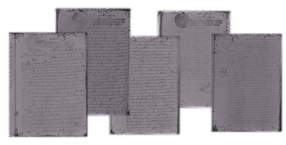
Figure 1: Example of corpus pages from books JMDB_4949 and JMBD_4950.

A first section of about 50 pages, which contains a kind of table of contents of the book, was also identified but not used in the present experiments. It is worth noting that each notarial act can contain from one to dozens of pages, and separating these acts is not straightforward. In future works, we plan to develop methods to also perform this task automatically, but for the present work we take the manual segmentation as given.

During the segmentation and labeling of the two protocol books, the experts found a total of 558 notarial acts, 296 from JMBD_4949 and 261 from JMBD_4950, belonging to 38 different types or classes. However, for most classes, only very few acts were available. To allow the classification results to be sufficiently reliable, only those classes having at least five acts in each book were taken into account.

This way, thirteen classes were retained as sufficiently representative and an ’other’ class was added to represent the remaining classes, making it possible to use 557 notarial acts (i.e., documents), and discarding just one.(EXPLICAR PORQUE)

The thirteen types (classes) we are finally left with are: Power of Attorney (P, from Spanish “Poder”), Letter of Payment (CP, “Carta de Pago”), Debenture (O, “Obligación”), Lease (A, “Arrendamiento”), Will (T, “Testamento”), Sale (V, “Venta”), Risk (R, “Riesgo”), Census (CEN, “Censo”), Deposit (DP, “Deposito”), Statement (D, “Declaración”), Cession (C, “Cesión”), Treaty of fact (TH, “Tratado de hecho”) and Redemption (RED, “Redención”),

Details of this dataset are shown in Table 1.

	JMBD_4949 & JMBD_4950
Classes	Nº docs.	Avg. pages per doc.	Min-max pages per doc.	Typical deviation	Total pages
P	240	3.34	2-24	3.45	803
CP	73	4.78	2-30	5.38	349
O	44	4.81	2-32	5.64	212
A	32	4.75	2-16	2.63	152
T	29	8.55	4-48	9.36	248
V	21	22.85	4-122	29.79	480
R	17	4.00	4-4	0.00	68
CEN	12	11.50	2-26	9.02	138
DP	10	3.80	2-8	1.88	38
D	10	2.40	2-4	0.80	24
C	6	5.33	2-14	3.94	32
TH	6	5.33	4-8	1.88	32
RED	1	12.00	12-12	0.0	12
OTHER	56	9.17	2-70	12.32	514
Total	557	5.56	2-122	9.14	3102

Table 1: Number of documents and page images for JMBD_4949 and JMBD_4950: per class, per document & class, and totals.

The machine learning task consists in training a model to classify each document into one of the $C=14$ classes considered.

5.2 Empirical settings

PrIx vocabularies typically contain huge amounts of pseudo-word hypotheses. However, many of these hypotheses have low relevance probability and most of the low-probability pseudo-words are not real words. Therefore, as a first step, the huge PrIx vocabulary was pruned out avoiding entries with less than three characters, as well as pseudo-words $v$ with too low estimated document frequency; namely, $E[m(v,\mathcal{X})]<1.0$. This resulted in a vocabulary $V$ of $559\,012$ pseudo-words for the two books considered in this work. Secondly, to retain the most relevant features, (pseudo-)words were sorted by decreasing values of IG and the first $n$ entries of the sorted list were selected to define a BOW vocabulary $V_{n}$. Exponentially increasing values of $n$ from $8$ up to $16\,384$ were considered in the experiments. Finally, a $\operatorname*{\operatorname*{Tf}\!\cdot\!\operatorname*{Idf}}$ $n$-dimensional vector was calculated for each document, $D\equiv X\in\mathcal{X}$. For experimental simplicity, $\operatorname*{\operatorname*{Tf}\!\cdot\!\operatorname*{Idf}}(v,D)$ was estimated just once all for all $v\in V$, using the normalized factor $f(D)\equiv E[n(X)]$ computed for all $v\in V$, rather than just $v\in V_{n}$.

For MLP classification, document vectors were normalized by subtracting the mean and dividing by the standard deviation, resulting in zero-mean and unit-variance input vectors. The parameters of each MLP architecture were initialized following [5] and trained according to the cross-entropy loss for 100 epochs using the SGD optimizer [15] with a learning rate of $0.01$. This configuration has been used for all the experiments presented in section 6.

6 Experiments and Results

The empirical work has focused on MLP classification of documents (handwritten notarial acts) of two books, JMBD_4949 and JMBD_4950. For the two books at the same time, we classify their documents (groups of images of handwritten pages) in the fourteen established classes in Sec. 5.

For this paper, two types of experiments have been performed. First, we performed a leave-one-out classification with the pages grouped by notarial acts and then, we performed another leave-one-out classification, but this time with the samples divided by pages and a subsequent vote to determine the class to which the notarial act belongs.

6.1 Groups

For this first experiment, we have made a leave one out classification with the pages grouped by notarial acts.

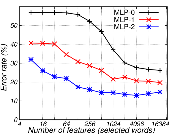
Figure 2: Leaving-one-out classification error rate for three classifiers for JMBD_4949 and JMBD_4950. 95% confidence intervals (not shown for clarity) are all smaller than $\pm 3.0\%$ for all the errors.

As shown in Figure 2, best results are obtained using MLP-2, archieving an error of 12.92% with a vocabulary of n = 4096 words. For this model we can see a degradation for lower and higher values of n. The rest of models not even come close to MLP-2 model, since the best result comes from MLP-1 and is 19.74 for n = 16384, which is far from the best result obtained with MLP-2.

Model complexity, in terms of numbers of parameters to train, grows with the number of features, $n$ as:

$$\centering\vspace{-0.2em}\text{MLP-0:}~{}5\,n+5~{}~{}~{}~{}\text{MLP-1:}~{}128\,n+773~{}~{}~{}~{}\text{MLP-2:}~{}128\,n+17\,285\vspace{-0.2em}\@add@centering$$

For all $n>64$, the least complex model is MLP-0, followed by MLP-1 and MLP-2. For $n=2\,048$, MLP-0, MLP-1 and MLP-2 have $10\,245$, $262\,917$ and $279\,429$ parameters, respectively. Therefore, despite the complexity of the model, MLP-2 is the best choice for the task considered in this work.

Table  6.1 shows the average confusion matrix and the specific error rate per class, using the best model (MLP-2) with the best vocabulary ($n$).

JMBD_4949 & JMBD_4950
	TH	C	D	DP	CE	R	V	T	A	O	CP	P	RE	OT	Total	Error (%)
TH	6	0	0	0	0	0	0	0	0	0	0	0	0	0	6	0.0
C	0	1	0	0	0	0	0	0	0	0	4	1	0	0	6	83.3
D	0	0	3	0	0	0	0	3	1	0	0	0	0	3	10	70.0
DP	0	0	0	9	0	0	1	0	0	0	0	0	0	0	10	10.0
CEN	0	0	0	1	7	0	0	0	0	0	0	0	0	4	12	41.6
R	0	0	0	0	0	17	0	0	0	0	0	0	0	0	17	0.0
V	1	0	0	0	0	0	18	0	0	0	1	0	0	1	21	14.3
T	0	0	0	0	1	0	0	26	0	0	0	1	0	1	29	10.3
A	0	0	0	0	0	0	0	0	29	0	1	0	0	2	32	9.4
O	0	0	0	0	0	0	0	0	1	33	1	3	0	6	44	25.0
CP	0	0	0	0	0	0	2	0	1	3	62	3	0	2	73	15.06
P	0	0	0	0	2	0	0	0	0	0	3	230	0	5	240	4.16
RED	0	0	0	0	1	0	0	0	0	0	0	0	0	0	1	100.0
OTHER	0	0	1	0	4	0	2	0	0	3	3	4	0	39	56	30.3

6.2 1-Page without voting

For this experiment, all the pages of the two files were classified one by one by means of leave one out.

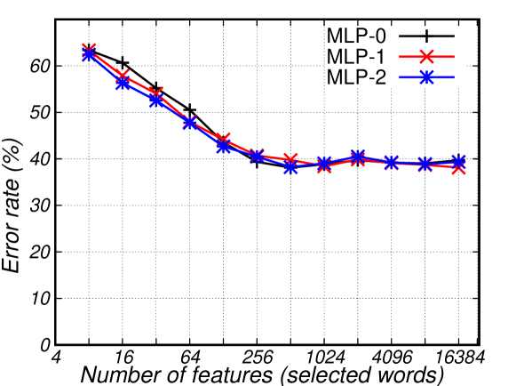
Figure 3: Leaving-one-out classification error rate for three classifiers for JMBD_4949 and JMBD_4950. 95% confidence intervals (not shown for clarity) are all smaller than $\pm 3.0\%$ for all the errors.

In this case, we can see in the Figure 3 a much higher error than in the previous experiment, since the pages have been sorted one by one and not by notarial acts. The best error rate is obtained with MLP-0 and MLP-1 for 512 and 16384 input words respectively, obtaining an error of 38.13%.

From these results we can conclude that page-by-page classification models would not be of great advance to the field of content based document classification. However, if we add to these models a vote between the pages of the same notarial act to determine the class to which it belongs, things change, as we will see in the next section.

6.3 1-Page with voting

Regarding this experiment, all the pages of the two files were classified one by one by means of leave one out, like the previous experiment, and then a vote was taken among the pages of each notarial act to determine to which class this act belongs.

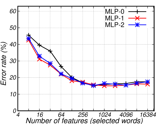
Figure 4: Leaving-one-out classification error rate for three classifiers for JMBD_4949 and JMBD_4950 with subsequent voting. 95% confidence intervals (not shown for clarity) are all smaller than $\pm 3.0\%$ for all the errors.

As we can see in Figure 4, the results this time are much better than in the previous case. Here again we find a tie between MLP-0 and MLP-1, both obtaining the same error rate, although for different number of input words.

While MLP-0 obtains an error rate of 15.06% for n = 512, MLP-1 obtains this same rate for n = 1024 and n = 2048, which is why despite obtaining the same result, the MLP-1 model would be a better option for this work, since we can also verify that MLP-1 always obtains a lower error than MLP-0, except on two occasions (n = 256 and n = 512).

As a result of these error rates, we can conclude that voting significantly improves model predictions. Since we have gone from unproductive models to ones that would be of great utility and advance for expert archivists.

7 Conclusions

We have presented and showcased an approach that is able to perform textual-content-based document classification directly on multi-page documents of untranscribed handwritten text images. Our method uses rather traditional techniques for plaintext document classification, estimating the required word frequencies from image probabilistic indexes. This way, we overcome the need to explicitly transcribe manuscripts, which is generally unfeasible for large collections.

The experimental results obtained with the proposed approach leave no doubt regarding its capabilities to model the textual contents of the page images and to discriminate among content-defined classes.

In our opinion, probabilistic indexing opens new avenues for research in textual-content-based image document classification. In future works, we plan to explore the use of other classification methods based on information extracted from probabilistic indexes. On the other hand, we aim to capitalize on the observation that fairly accurate classification can be achieved with relatively small vocabularies, down to 64 words in the task considered in this paper. In this direction, we will explore the use of information gain and/or $\operatorname*{\operatorname*{Tf}\!\cdot\!\operatorname*{Idf}}$ values estimated for probabilistic index (pseudo-)words to derive a small set of words that semantically describes the contents of each bundle of manuscripts. This would allow the automatic or semi-automatic creation of metadata which could be extremely useful for scholars and the general public searching for historical information in archived manuscripts.

References

- [1] Aggarwal, C.C., Zhai, C.: Mining text data. Springer Science & Business Media (2012)
- [2] Aizawa, A.: An information-theoretic perspective of tf–idf measures. Inf. Proc. & Management 39(1), 45–65 (2003)
- [3] Bluche, T., Hamel, S., Kermorvant, C., Puigcerver, J., Stutzmann, D., Toselli, A.H., Vidal, E.: Preparatory KWS Experiments for Large-Scale Indexing of a Vast Medieval Manuscript Collection in the HIMANIS Project. In: 14th IAPR Int. Conf. on Document Analysis and Recognition (ICDAR). vol. 01, pp. 311–316 (Nov 2017)
- [4] E. Vidal et al.: The carabela project and manuscript collection: Large-scale probabilistic indexing and content-based classification. In: 16th ICFHR (Sep 2020)
- [5] Glorot, X., Bengio, Y.: Understanding the difficulty of training deep feedforward neural networks. Journal of Machine Learning Research 9, 249–256 (2010)
- [6] Ikonomakis, M., Kotsiantis, S., Tampakas, V.: Text classification using machine learning techniques. WSEAS transactions on computers 4,8, 966–974 (2005)
- [7] Ioffe, S., Szegedy, C.: Batch Normalization: Accelerating Deep Network Training by Reducing Internal Covariate Shift (2015)
- [8] Joachims, T.: A probabilistic analysis of the Rocchio algorithm with TFIDF for text categorization. Tech. rep., Carnegie-mellon univ pittsburgh pa dept of computer science (1996)
- [9] Khan, A., Baharudin, B., Lee, L.H., Khan, K.: A review of machine learning algorithms for text-documents classification. Journal of advances in information technology 1(1), 4–20 (2010)
- [10] Lang, E., Puigcerver, J., Toselli, A.H., Vidal, E.: Probabilistic indexing and search for information extraction on handwritten german parish records. In: 2018 16th International Conference on Frontiers in Handwriting Recognition (ICFHR). pp. 44–49 (Aug 2018)
- [11] Manning, C.D., Raghavan, P., Schtze, H.: Introduction to Information Retrieval. Cambridge University Press, New York, NY, USA (2008)
- [12] Prieto, J.R., Bosch, V., Vidal, E., Alonso, C., Orcero, M.C., Marquez, L.: Textual-content-based classification of bundles of untranscribed manuscript images. In: 2020 25th International Conference on Pattern Recognition (ICPR). pp. 3162–3169. IEEE (2021)
- [13] Puigcerver, J.: A Probabilistic Formulation of Keyword Spotting. Ph.D. thesis, Univ. Politècnica de València (2018)
- [14] Romero, V., Toselli, A.H., Vidal, E., Sánchez, J.A., Alonso, C., Marqués, L.: Modern vs diplomatic transcripts for historical handwritten text recognition. In: International Conference on Image Analysis and Processing. pp. 103–114. Springer (2019)
- [15] Ruder, S.: An overview of gradient descent optimization algorithms 14, 2–3 (2017)
- [16] Salton, G., Buckley, C.: Term-weighting approaches in automatic text retrieval. Inf. Proc. & Management 24(5), 513/523 (1988)
- [17] Sánchez, J.A., Romero, V., Toselli, A.H., Villegas, M., Vidal, E.: A set of benchmarks for handwritten text recognition on historical documents. Pattern Recognition 94, 122–134 (2019)
- [18] Toselli, A., Romero, V., Vidal, E., Sánchez, J.: Making two vast historical manuscript collections searchable and extracting meaningful textual features through large-scale probabilistic indexing. In: 2019 15th IAPR Int. Conf. on Document Analysis and Recognition (ICDAR) (2019)
- [19] Toselli, A.H., Vidal, E., Puigcerver, J., Noya-García, E.: Probabilistic multi-word spotting in handwritten text images. Pattern Analysis and Applications 22(1), 23–32 (2019)
- [20] Toselli, A.H., Vidal, E., Romero, V., Frinken, V.: HMM Word Graph based Keyword Spotting in Handwritten Document Images. Information Sciences 370-371, 497–518 (2016)
- [21] Vidal, E., Toselli, A.H., Puigcerver, J.: A probabilistic framework for lexicon-based keyword spotting in handwritten text images. Tech. rep., UPV (2017)