A Mean Field Game Approach to Equilibrium Consumption under External Habit Formation

Abstract

This paper studies the equilibrium consumption under external habit formation in a large population of agents. We first formulate problems under two types of conventional habit formation preferences, namely linear and multiplicative external habit formation, in a mean field game framework. In a log-normal market model with the asset specialization, we characterize one mean field equilibrium in analytical form in each problem, allowing us to understand some quantitative properties of the equilibrium strategy and conclude distinct financial implications caused by different consumption habits from a mean field perspective. In each problem with $n$ agents, we then construct an approximate Nash equilibrium for the $n$-player game using the obtained mean field equilibrium when $n$ is sufficiently large. The explicit convergence order in each problem can also be obtained.

Mathematics Subject Classification (2020): 49N80, 91A15, 91B42, 91B50, 91B10

Keywords: Catching up with the Joneses, linear habit formation, multiplicative habit formation, mean field equilibrium, approximate Nash equilibrium

1 Introduction

To reconcile the observed equity premium puzzle, the time non-separable habit formation preference has been proposed (see Constantinides (1990)) as a new paradigm for measuring individual’s consumption satisfaction and risk aversion over the past decades. The dependence of the utility on the entire past consumption path can partially explain why consumers’ reported sense of well-being often seems more related to recent changes than to the absolute levels. The time non-separable structure can also help to explain the well documented smoothness in consumption data. Some recent developments in internal habit formation for an individual investor can be found in Detemple and Zapatero (1992), Englezos and Karatzas (2009), Schroder and Skiadas (2002), Yu (2015), Yu (2017), Guan et al. (2020), van Bilsen et al. (2020), Yang and Yu (2022), Bahman et al. (2022) among others.

Another research direction with fruitful outcomes is to extend from a single agent’s optimal consumption problem to the study of equilibrium consumption behavior with a group of agents, in which each individual’s habit level depends on the average of the aggregate consumption from all peers in the economy; see Abel (1990), Detemple and Zapatero (1991), Abel (1999), Campbell and Cochrane (1999) and references therein. The so-called “catching up with the Joneses” has been widely used to refer to the external habit formation preferences and depict the flavor of competition in the equilibrium problem as each agent chooses the relative consumption by competing with the historical consumption record from others. In the literature with $n$ agents, the linear external habit formation and the multiplicative external habit formation have been two dominating preferences thanks to their mathematical tractability and simple structure for financial interpretations. The linear external habit formation preference (see, for example, Constantinides (1990), Detemple and Zapatero (1991)) measures the difference between the current consumption rate and the average of the aggregate consumption from all agents under the CRRA utility, featuring the addictive consumption habits in the sense that each agent can not tolerate the consumption to fall below the external habit level induced by the infinite marginal utility. On the other hand, the multiplicative habit formation preference (see, for example, Abel (1990), Campbell and Cochrane (1999), Carroll (2000)) is defined on the ratio of the current consumption and the average of the aggregate consumption. It is conventionally referred to non-addictive habit formation as the agent can bear the consumption plan to be lower than the habit level from time to time and may strategically suppress the consumption temporarily to accumulate higher wealth from the financial market.

In this paper, we revisit these two types of external habit formation preferences, however, from the relative performance and mean field game perspective. We aim to investigate the equilibrium consumption behavior with a continuum of agents when each agent focuses on the investment on the individual stock or asset class. In particular, we will first study the equilibrium consumption as a mean field game problem when the market is populated by infinitely many heterogenous agents. We then establish some connections to the model with $n$ agents by providing the approximation to the Nash equilibrium when $n$ is sufficiently large. In sharp contrast to the aforementioned studies on equilibrium consumption under external habit formation, we will not characterize the excessive return of the risky asset as the equilibrium output (see, for example, Abel (1990), Detemple and Zapatero (1991), Abel (1999)). Instead, we regard the external habit formation as the relative performance benchmark and examine the associated $n$-player game and mean field game (MFG) in the same spirit of Lacker and Zariphopoulou (2019) and Lacker and Soret (2020). We can then take advantage of the tractability in the mean field game formulation when the influence of each agent on the population is negligible; see Huang et al. (2006) and Lasry and Lions (2007) and many subsequent studies. In each problem with linear habit formation and multiplicative habit formation respectively, we can obtain one mean field equilibrium in an elegant analytical form, allowing us to investigate some impacts by model parameters and the external consumption habits and discuss some new and interesting financial implications. Moreover, we can further construct the approximate Nash equilibrium in the model with $n$ agents using the simple mean field equilibrium with the explicit order of approximation error, which can reduce the dimensionality significantly in the practical implementation of the $n$-player game.

On the other hand, the present paper is also an important add-on to the literature of relative performance and competition games by featuring our path-dependent competition benchmark. The research on $n$-player games and mean field games under relative performance has been active in recent years. To name a few recent studies, we refer to Espinosa and Touzi (2015), Lacker and Zariphopoulou (2019), Lacker and Soret (2020), Dos Reis and Platonov (2020), Fu et al. (2020), Hu and Zariphopoulou (2021), Bo et al. (2021) among others. Unlike the previous research, the external habit formation process in the present paper is generated by the weighted average integral of consumption controls from all competitors, which gives rise to some new challenges in the proof of the consistency condition for the conjectured mean field equilibrium. In addition, in the construction and verification of the approximate Nash equilibrium for the $n$-player game, more efforts are needed to ensure that the addictive habit constraint is satisfied in the problem with linear habit formation and the well-posedness of the problem with multiplicative habit formation. Some technical arguments are also required to derive some estimations and to show convergence results due to the path-dependent feature in the external habit formation. In numerical illustrations, thanks to the analytical form of the mean field equilibrium and the approximate Nash equilibrium, we can make some new and interesting comparison analysis on quantitative impacts by two types of external habit formation preferences and highlight their distinct financial implications.

The rest of the paper is organized as follows. In Section 2, we introduce the $n$-player game problems under linear and multiplicative habit formation preferences when the asset specialization is applied to each agent. In Section 3, we formulate two MFG problems under two types of external habit formation with infinitely many agents. A mean field equilibrium in each problem is established in analytical form. Some numerical illustrations and sensitivity analysis of the mean field equilibrium as well as their financial implications are presented in Section 4. In Section 5, we construct and verify an approximate Nash equilibrium in each $n$-player game when $n$ is sufficiently large using the mean field equilibrium and derive the explicit order of the approximation error. Some conclusions and future research directions are given in Section 6.

2 The Market Model

For a finite horizon $T>0$, let $(\Omega,\mathcal{F},\mathbb{F},\mathbb{P})$ be a filtered probability space, where the filtration $\mathbb{F}=(\mathcal{F}_{t})_{t\in[0,T]}$ satisfies the usual conditions. We consider a market model consisting of one riskless bond and $n$ risky assets, in which there are $n$ heterogeneous agents who dynamically invest and consume up to the finite horizon $T$. Without loss of generality, the interest rate of the riskless bond is assumed be $r=0$ by changing of numéraire.

Similar to Lacker and Zariphopoulou (2019), the asset specialization to each agent is assumed that the agent $i$ can only invest in the risky asset $S^{i}=(S^{i}_{t})_{t\in[0,T]}$ whose price process follows

$$dS^{i}_{t}=S^{i}_{t}\mu_{i}dt+S^{i}_{t}\sigma_{i}dW^{i}_{t},\ \ i=1,\ldots,n,$$ (2.1)

where $W=(W_{t}^{1},\ldots,W_{t}^{n})_{t\in[0,T]}$ is an $n$-dimensional $\mathbb{F}$-adapted Brownian motion.

For $i=1,\ldots,n$, let $(\pi^{i},C^{i})=(\pi^{i}_{t},C_{t}^{i})_{t\in[0,T]}$ be an $\mathbb{F}$-adapted process, where $\pi^{i}$ represents the dynamic proportion of wealth that the agent $i$ allocates in the risky asset $S^{i}$ and $C^{i}$ represents the consumption rate process of agent $i$. We also denote the consumption-to-wealth proportion $c_{t}^{i}:=C^{i}_{t}/X^{i}_{t}$ if $X_{t}^{i}>0$. The resulting self-financing wealth process $X^{i}=(X^{i}_{t})_{t\in[0,T]}$ of agent $i$ is governed by

$$\frac{dX^{i}_{t}}{X^{i}_{t}}=\pi^{i}_{t}\mu_{i}dt+\pi^{i}_{t}\sigma_{i}dW^{i}_{t}-c^{i}_{t}dt,\quad t\in[0,T],$$ (2.2)

with the initial wealth $X^{i}_{0}=x^{i}_{0}>0$.

The so-called habit formation process $Z^{i}=(Z_{t}^{i})_{t\in[0,T]}$ of agent $i$ generated by the consumption rate process $C^{i}=(C_{t}^{i})_{t\in[0,T]}$ is defined by

$$dZ^{i}_{t}=-\delta_{i}(Z^{i}_{t}-C^{i}_{t})dt,\quad Z_{0}^{i}=z^{i}_{0}>0,$$

where $z^{i}_{0}$ stands for the initial habit. It follows that

$$Z^{i}_{t}=e^{-\delta_{i}t}\left(z^{i}_{0}+\int_{0}^{t}\delta_{i}e^{\delta_{i}s}C^{i}_{s}ds\right),\quad t\in[0,T].$$ (2.3)

Here, the habit intensity parameter $\delta_{i}>0$ depicts how much the habit is influenced by the recent consumption path comparing with the initial habit level.

For the group of $n$ agents in the financial market, let us define their average habit formation process by

$$\bar{Z}_{t}^{n}:=\frac{1}{n}\sum_{i=1}^{n}Z_{t}^{i},\quad t\in[0,T],$$ (2.4)

which depicts the average of aggregate consumption trend in the economy.

We now introduce the agent’s optimal relative consumption problem by taking into account the average habit formation from all $n$ peers. In particular, we consider two types of conventional external habit formation preferences, namely the linear habit formation and the multiplicative habit formation. For the $i$-th agent, the optimal relative consumption problem with the linear external habit formation is defined by

$$\max_{(\pi^{i},c^{i})\in\mathcal{A}^{l,i}(x^{i}_{0})}J_{i}^{l}(\bm{\pi},\bm{c}) :=\max_{(\pi^{i},c^{i})\in\mathcal{A}^{l,i}(x^{i}_{0})}\mathbb{E}\left[\int_{0}^{T}U_{i}\left(c^{i}_{t}X_{t}^{i}-\bar{Z}^{n}_{t}\right)dt+U_{i}(X_{T}^{i})\right],$$ (2.5)

and the optimal consumption problem with the multiplicative external habit formation is defined by

$$\max_{(\pi^{i},c^{i})\in\mathcal{A}^{m,i}(x^{i}_{0})}J_{i}^{m}(\bm{\pi},\bm{c}) :=\max_{(\pi^{i},c^{i})\in\mathcal{A}^{m,i}(x^{i}_{0})}\mathbb{E}\left[\int_{0}^{T}U_{i}\left(\frac{c^{i}_{t}X_{t}^{i}}{(\bar{Z}_{t}^{n})^{\alpha_{i}}}\right)dt+U_{i}(X_{T}^{i})\right],$$ (2.6)

where $(\bm{\pi},\bm{c})=((\pi^{1},c^{1}),\ldots,(\pi^{n},c^{n}))$, $\alpha_{i}\in(0,1]$ represents the habit persistence in the multiplicative habit formation that can also be understood as the competition level of the relative performance, and $U_{i}:\mathbb{R}_{+}\to\mathbb{R}_{+}$ ($i=1,\ldots,n$) is the power utility of agent $i$ that

$$U_{i}(y)=\frac{1}{p_{i}}y^{p_{i}},\quad p_{i}\in(0,1),\quad y\geq 0.$$ (2.7)

For two types of external habit formation preferences, we stress that the admissible control sets are different. In problem (2.5) under the linear habit formation, the external consumption habits are addictive in the sense that $C^{i}_{t}=c^{i}_{t}X^{i}_{t}\geq\bar{Z}^{n}_{t}$ for $t\in[0,T]$ a.s. because of the infinite marginal utility. Therefore, we define ${\cal A}^{l,i}(x^{i}_{0})$ as the set of $\mathbb{F}$-adapted (r.c.l.l.) consumption-portfolio pairs $(\pi^{i},c^{i})$ such that $c^{i}_{t}X^{i}_{t}\geq\bar{Z}^{n}_{t}$ and no bankruptcy condition holds that $X^{i}_{t}>0$ a.s. for $t\in[0,T]$. To ensure that the admissible set ${\cal A}^{l,i}(x^{i}_{0})$ is non-empty, we additionally require that $x^{i}_{0}>z^{i}_{0}T$ such that the initial wealth $x^{i}_{0}$ of the agent $i$ is sufficiently large to support the consumption under addictive habit constraint.

On the other hand, in view of the ratio form in problem (2.6) under multiplicative habit formation, the consumption can fall below the habit level and the external habit is non-addictive. Therefore, we shall define ${\cal A}^{m,i}(x^{i}_{0})$ as the set of $\mathbb{F}$-adapted (r.c.l.l.) consumption-portfolio pairs $(\pi^{i},c^{i})$ such that $c^{i}_{t}\geq 0$, a.s. and no bankruptcy is allowed that $X^{i}_{t}>0$ a.s. for $t\in[0,T]$. For the well-posedness of the problem, it is additionally assumed in ${\cal A}^{m,i}(x^{i}_{0})$ that the uniform boundedness condition holds that $\sup_{i\geq 1}\sup_{t\in[0,T]}|\pi_{t}^{i}|\vee|c_{t}^{i}|<\infty$, a.s. and the initial habit is strictly positive that $z^{i}_{0}>\epsilon$ for some constant $\epsilon>0$.

For technical convenience and ease of presentation, we shall make the following assumption throughout the paper.

• $\bm{(A_{h})}$: Assume that all agents are homogenous in their initial wealth, the initial habit, the habit discounting factor and the habit persistence level such that $(x^{i}_{0},z^{i}_{0},\delta_{i},\alpha_{i})=(x_{0},z_{0},\delta,\alpha)\in\mathbb{R}_{+}^{3}\times{(0,1]}$, $i=1,\ldots,n$. Additionally, in problem (2.5), it is assumed that $x_{0}>z_{0}T$; In problem (2.6), it is assumed that $z_{0}>\epsilon$ for some constant $\epsilon>0$.

Note that the heterogeneity of $n$ agents in the present paper is captured via their different type vectors $o_{i}:=(\mu_{i},\sigma_{i},p_{i})\in{\cal O}:=\mathbb{R}\times\mathbb{R}_{+}\times(0,1)$.

3 Mean Field Game Problems

We now proceed to formulate the mean field games under linear and multiplicative external habit formation when the number of agents grows to infinity. The type vector $o_{i}=(\mu_{i},\sigma_{i},p_{i})$, $i=1,\ldots,n$, induces an empirical measure on the type space ${\cal O}$ given by

$${\rm m}_{n}(A):=\frac{1}{n}\sum_{i=1}^{n}\mathbf{1}_{A}(o_{i}),$$

for Borel sets $A\subset{\cal O}$ (i.e., $A\in{\cal B}({\cal O})$). The following assumption is needed to formulate the MFG problems:

• $\bm{(A_{o})}$: there exists a random type vector $o=(\mu,\sigma,p)\in\mathcal{O}$ with the distribution ${\rm m}\in{\cal P}({\cal O})$ such that $\int_{{\cal O}}fd{\rm m}_{n}\rightarrow\int_{{\cal O}}fd{\rm m}$, as $n\to\infty$, for every bounded and continuous function $f$ on ${\cal O}$ (i.e., $f\in C_{b}({\cal O})$).

For the random type vector $o=(\mu,\sigma,p)$ given in the assumption $\bm{(A_{o})}$, the wealth process of a representative agent is giverned by

$$\frac{dX_{t}}{X_{t}}=\pi_{t}\mu dt+\pi_{t}\sigma dW_{t}-c_{t}dt,\quad X_{0}=x_{0}.$$ (3.1)

For $n$ sufficiently large, we may approximate $\bar{Z}^{n}=(\bar{Z}^{n}_{t})_{t\in[0,T]}$ by a deterministic function $\bar{Z}=(\bar{Z}_{t})_{t\in[0,T]}$, and this can be heuristically justified by the law of large numbers as long as the individual controls satisfy some mild conditions. To this purpose, let the deterministic function $\bar{Z}=(\bar{Z}_{t})_{t\in[0,T]}\in{\cal C}_{T}:=C([0,T];\mathbb{R}_{+})$ denote the approximation of the average habit formation process $\bar{Z}^{n}=(\bar{Z}^{n}_{t})_{t\in[0,T]}$ as $n\to\infty$.

3.1 Mean field equilibrium under linear habit formation

In this section, we formulate and study the MFG problem under linear external habit formulation associated to the $n$-player problem considered in (2.5). Given a deterministic function $\bar{Z}=(\bar{Z}_{t})_{t\in[0,T]}$ as the approximation of $\bar{Z}^{n}=(\bar{Z}^{n}_{t})_{t\in[0,T]}$ when $n\to\infty$, the dynamic version of the objective function for a representative agent under linear external habit formulation is defined by

$$\bar{J}^{l}((\pi,c),t,x;\bar{Z}):=\mathbb{E}_{t,x}\left[\int_{t}^{T}\frac{1}{p}(c_{s}X_{s}-\bar{Z}_{s})^{p}ds+\frac{(X_{T})^{p}}{p}\right],$$ (3.2)

where $\mathbb{E}_{t,x}=\mathbb{E}[\cdot|X_{t}=x]$. Accordingly, the optimal control problem is given by

$$\sup_{(\pi,c)\in{\cal A}^{l}(x)}\bar{J}^{l}((\pi,c),t,x;\bar{Z})=\mathbb{E}_{\rm m}\left[V^{l}(t,x,o)\right]:=\int_{{\cal O}}V^{l}(t,x,o){\rm m}(do),$$ (3.3)

where ${\cal A}^{l}(x)$ is the dynamic admissible control set of $\mathbb{F}$-adapted consumption-portfolio pairs $(\pi,c)$ such that $c_{s}X_{s}\geq\bar{Z}_{s}$, $s\in[t,T]$, and no bankruptcy condition holds that $X_{s}>0$ a.s. for $s\in[t,T]$, and $V^{l}(t,x,o)$ is the value function for a given random type vector $o$.

Recall that $x_{0}>z_{0}T$ in the assumption $\bm{(A_{h})}$. Let us denote

$${\cal C}_{T,x_{0}}:=\left\{\bar{Z}=(\bar{Z}_{t})_{t\in[0,T]}\in{\cal C}_{T}:\int_{0}^{T}\bar{Z}_{t}dt<x_{0}\right\}.$$ (3.4)

We then formally give the definition of the mean field equilibrium as below.

Definition 3.1.

For a given $\bar{Z}=(\bar{Z}_{t})_{t\in[0,T]}\in{\cal C}_{T,x_{0}}$, let $(\pi^{*,\bar{Z}},c^{*,\bar{Z}})\in{\cal A}^{l}(x_{0})$ be the best response strategy to the stochastic control problem (3.3) from the initial time $t=0$. The strategy $(\pi^{l},c^{l}):=(\pi^{*,\bar{Z}^{l}},c^{*,\bar{Z}^{l}})$ is called a mean field equilibrium if it is the best response to itself in the sense that $\bar{Z}^{l}_{t}=z_{0}e^{-\delta t}+\int_{0}^{t}\delta e^{\delta(s-t)}\mathbb{E}[c_{s}^{l}X_{s}^{l,\bar{Z}^{l}}]ds$, $t\in[0,T]$, where $X^{l,\bar{Z}^{l}}=(X_{t}^{l,\bar{Z}^{l}})_{t\in[0,T]}$ is the wealth process under the best response control $(\pi^{l},c^{l})$ with $X_{0}^{l,\bar{Z}^{l}}=x_{0}$.

By Definition 3.1, we shall first find the best response strategy to the stochastic control problem (3.3) for a given function $\bar{Z}=(\bar{Z}_{t})_{t\in[0,T]}\in{\cal C}_{T,x_{0}}$. Let $o=(\mu,\sigma,p)$ now represent a deterministic sample from its random type distribution. Using dynamic program arguments, we can derive the associated HJB equation of the value function $V^{l}(t,x):=V^{l}(t,x,o)$ on the effective domain $\{(t,x)\in[0,T]\times\mathbb{R}_{+}:x>\int_{t}^{T}\bar{Z}_{s}ds\}$ that

$$\partial_{t}V^{l}+\sup_{\pi\in\mathbb{R}}\left(\mu\pi x\partial_{x}V^{l}+\frac{\sigma^{2}}{2}\pi^{2}x^{2}\partial_{x}^{2}V^{l}\right)+\sup_{c\geq 0}\left(\frac{1}{p}(cx-\bar{Z}_{t})^{p}-cx\partial_{x}V^{l}\right)=0,$$ (3.5)

with the terminal condition $V^{l}(T,x)=\frac{1}{p}x^{p}$ for $x>0$.

Lemma 3.1.

Let $\bar{Z}=(\bar{Z}_{t})_{t\in[0,T]}\in{\cal C}_{T,x_{0}}$. The classical solution of the HJB equation (3.5) on the effective domain $\{(t,x)\in[0,T]\times\mathbb{R}_{+}:x>\int_{t}^{T}\bar{Z}_{s}ds\}$ admits the closed-form that

$$V^{l}(t,x)=\frac{1}{p}\left(x-\int_{t}^{T}\bar{Z}_{s}ds\right)^{p}g^{l}(t),$$ (3.6)

where

$$g^{l}(t):=\left[\left(1+\frac{1}{a}\right)e^{a(T-t)}-\frac{1}{a}\right]^{1-p},\quad\quad a:=\frac{1}{2}\frac{\mu^{2}}{\sigma^{2}}\frac{p}{(1-p)^{2}}>0.$$ (3.7)

The feedback functions of the optimal investment and consumption to the problem (3.3) from the initial time are given by

$$\pi^{*,\bar{Z}}(t,x) =\frac{\mu}{(1-p)\sigma^{2}x}\left(x-\int_{t}^{T}\bar{Z}_{s}ds\right),\quad c^{*,\bar{Z}}(t,x)=\frac{1}{x}\left[\bar{Z}_{t}+\left(x-\int_{t}^{T}\bar{Z}_{s}ds\right)g^{l}(t)^{\frac{1}{p-1}}\right],$$ (3.8)

and the controlled optimal wealth process satisfies $X^{*,\bar{Z}}_{t}>\int_{t}^{T}\bar{Z}_{s}ds$, a.s., for all $t\in[0,T]$.

Proof.

Suppose that there exists a classical solution $V$ to the HJB equation (3.5) on the effective domain $\{(t,x)\in[0,T]\times\mathbb{R}_{+}:x>\int_{t}^{T}\bar{Z}_{s}ds\}$ that is strictly concave (i.e., $\partial_{x}^{2}V^{l}<0$) and $\partial_{x}V^{l}>0$. The first-order condition gives the optimal (feedback) investment-consumption strategies that

$$\pi^{*,\bar{Z}}(t,x) =-\frac{\mu}{\sigma^{2}}\frac{\partial_{x}V^{l}(t,x)}{x\partial_{x}^{2}V^{l}(t,x)},\quad c^{*,\bar{Z}}(t,x)=\frac{1}{x}\left(\bar{Z}_{t}+(\partial_{x}V^{l})^{\frac{1}{p-1}}\right).$$

Plugging them into the HJB equation (3.5), we obtain that

$$\partial_{t}V^{l}-\frac{\mu^{2}}{2\sigma^{2}}\frac{(\partial_{x}V^{l})^{2}}{\partial_{x}^{2}V^{l}}-\bar{Z}_{t}\partial_{x}V^{l}+\frac{1-p}{p}(\partial_{x}V^{l})^{\frac{p}{p-1}}=0.$$

We conjecture that the value function satisfies the form $V^{l}(t,x)=\frac{(x-f(t))^{p}}{p}g^{l}(t)$, where $f(t):=\int_{t}^{T}\bar{Z}_{s}ds$ and $t\to g^{l}(t)$ is a positive function satisfying $g^{l}(T)=1$. Plugging the expression of $V^{l}(t,x)$ into the HJB equation, we arrive at

$$\frac{1}{p}(g^{l})^{\prime}(t)-\frac{\mu^{2}}{2\sigma^{2}(p-1)}g^{l}(t)+\frac{1-p}{p}(g^{l}(t))^{\frac{p}{p-1}}=0.$$ (3.9)

Note that (3.9) is a Bernoulli ODE. To solve this ODE, let us consider $g^{l}(t)=(u(t))^{1-p}$ for $t\in[0,T]$. Then $u(t)$ satisfies the following linear ODE:

$$u^{\prime}(t)+\frac{\mu^{2}p}{2\sigma^{2}(1-p)^{2}}u(t)+1=0,\quad u(T)=1.$$ (3.10)

This yields that $u(t)=(1+\frac{1}{a})e^{a(T-t)}-\frac{1}{a}$ with $a=\frac{p\mu^{2}}{2(1-p)^{2}\sigma^{2}}>0$. Therefore, we can find an explicit classical solution to the HJB equation on the domain $\{(t,x)\in[0,T]\times\mathbb{R}_{+}:x>\int_{t}^{T}\bar{Z}_{s}ds\}$ that

$$V^{l}(t,x)=\frac{(x-f(t))^{p}}{p}g^{l}(t)=\frac{1}{p}\left(x-\int_{t}^{T}\bar{Z}_{s}ds\right)^{p}\left[\left(1+\frac{1}{a}\right)e^{a(T-t)}-\frac{1}{a}\right]^{1-p},$$

which satisfies $\partial_{x}^{2}V^{l}<0$ and $\partial_{x}V^{l}>0$ .

We can then follow some standard arguments to prove the verification theorem and conclude that the optimal controls $(\pi^{x,\bar{Z}},c^{*,\bar{Z}})$ of the problem (3.3) are given in feedback form by (3.8) as long as we can show that the resulting wealth process $X^{*,\bar{Z}}$ under $(\pi^{*,\bar{Z}},c^{*,\bar{Z}})$ satisfies the constraint $X_{t}^{*,\bar{Z}}>\int_{t}^{T}\bar{Z}_{s}ds$, $t\in[0,T]$, such that $(\pi^{*,\bar{Z}}(t,X_{t}^{*,\bar{Z}}),c^{*,\bar{Z}}(t,X_{t}^{*,\bar{Z}})$ is an admissible control. That is, we need to show the existence of a strong solution to the SDE

$$\frac{dX_{t}^{*,\bar{Z}}}{X_{t}^{*,\bar{Z}}}=\pi^{*,\bar{Z}}_{t}\mu dt+\pi^{*,\bar{Z}}_{t}\sigma dW_{t}-c_{t}^{*,\bar{Z}}dt,\quad X_{0}^{*,\bar{Z}}=x_{0},$$ (3.11)

which evolves in the effective domain $\{(t,x)\in[0,T]\times\mathbb{R}_{+}:x>\int_{t}^{T}\bar{Z}_{s}ds\}$. To this end, let us consider $Y_{t}^{*,\bar{Z}}:=X_{t}^{*,\bar{Z}}-\int_{t}^{T}\bar{Z}_{s}ds$, $t\in[0,T]$. We deduce from (3.11) that

$$\frac{dY_{t}^{*,\bar{Z}}}{Y_{t}^{*,\bar{Z}}}=\left[\frac{\mu^{2}}{(1-p)\sigma^{2}}-g^{l}(t)^{\frac{1}{p-1}}\right]dt+\frac{\mu}{(1-p)\sigma}dW_{t},\quad Y_{0}^{*,\bar{Z}}=x_{0}-\int_{0}^{T}\bar{Z}_{s}ds.$$ (3.12)

It follows that $Y_{t}^{*,\bar{Z}}$ is a GBM, and the SDE (3.11) admits a strong solution. Moreover, $X_{t}^{*,\bar{Z}}>\int_{t}^{T}\bar{Z}_{s}ds$ indeed holds thanks to the condition $\int_{0}^{T}\bar{Z}_{s}ds<x_{0}$ using the fact that $\bar{Z}\in{\cal C}_{T,x_{0}}$. ∎

We next examine the fixed point problem from the consistence condition in Definition 3.1 that

$$\bar{Z}^{l}_{t}=e^{-\delta t}\left\{z_{0}+\int_{0}^{t}\delta e^{\delta s}\mathbb{E}[c_{s}^{l}X_{s}^{l,\bar{Z}^{l}}]ds\right\},\quad t\in[0,T].$$ (3.13)

For $t\in[0,T]$, recall that $Y_{t}^{*,\bar{Z}}=X_{t}^{*,\bar{Z}}-\int_{t}^{T}\bar{Z}_{s}ds$ is a GBM that satisfies (3.12). We have that

$$\mathbb{E}\left[Y_{t}^{*,\bar{Z}}\right]=\left(x_{0}-\int_{0}^{T}\bar{Z}_{s}ds\right)\exp\left\{\int_{0}^{t}\left(\frac{\mu^{2}}{(1-p)\sigma^{2}}-g^{l}(s)^{\frac{1}{p-1}}\right)ds\right\}.$$ (3.14)

With the help of (3.14), the consistency condition (3.13) for $\bar{Z}=(\bar{Z}_{t})_{t\in[0,T]}$ can be written as

$$d\bar{Z}_{t} =\delta\mathbb{E}\left[X_{t}^{*,\bar{Z}}-\int_{t}^{T}\bar{Z}_{s}ds\right]g^{l}(t)^{\frac{1}{p-1}}dt$$

$$=\delta\left(x_{0}-\int_{0}^{T}\bar{Z}_{s}ds\right)\exp\left\{\int_{0}^{t}\left(\frac{\mu^{2}}{(1-p)\sigma^{2}}-g^{l}(s)^{\frac{1}{p-1}}\right)ds\right\}g^{l}(t)^{\frac{1}{p-1}}dt,\quad\bar{Z}_{0}=z_{0}.$$ (3.15)

We then have the next result.

Proposition 3.1.

There exists a unique deterministic fixed point $\bar{Z}^{l}=(\bar{Z}^{l}_{t})_{t\in[0,T]}\in{\cal C}_{T,x_{0}}$ to Eq. (3.1), and hence $(\pi^{l},c^{l})=(\pi^{*,\bar{Z}^{l}},c^{*,\bar{Z}^{l}})$ is a mean field equilibrium, where $(\pi^{*,\bar{Z}},c^{*,\bar{Z}})$ is defined in (3.8) for a given $\bar{Z}$.

Proof.

Let us define that, for all $(t,Z)\in[0,T]\times{\cal C}_{T}$,

$$\Phi(t,Z) :=z_{0}+\delta\left(x_{0}-\int_{0}^{T}Z_{u}du\right)\int_{0}^{t}{\phi}(s)ds,$$ (3.16)

where ${\phi}(t):=\exp\{\int_{0}^{t}(\frac{\mu^{2}}{(1-p)\sigma^{2}}-g(u)^{\frac{1}{p-1}})du\}g^{l}(t)^{\frac{1}{p-1}}$. In light of (3.16), for any $Z^{1},Z^{2}\in{\cal C}_{T}$, we have that

$$\left\|\Phi(\cdot,Z^{1})-\Phi(\cdot,Z^{2})\right\|_{T} \leq\delta\left(\int_{0}^{T}|Z^{1}_{u}-Z_{u}^{2}|du\right)\left(\int_{0}^{T}\phi(t)dt\right)$$

$$\leq\delta C(T)\|Z^{1}-Z^{2}\|_{T},$$ (3.17)

where $C(T):=\delta T(\int_{0}^{T}\phi(t)dt)$. Note that $T\to C(T)$ is continuous on $\mathbb{R}_{+}$ and it satisfies $\lim_{T\to 0}C(T)=0$. Then, we can choose $t_{1}\in(0,T]$ small enough such that $C(t_{1})\in(0,1)$. Thus, ${\Phi}$ is a contraction map on ${\cal C}_{t_{1}}$ by (3.1), and hence there exists a unique fixed point of $\Phi$ on $[t_{0},t_{1}]$ with $t_{0}=0$. Note that $T\to C(T)$ is independent of $z$. Then, we can apply this similar argument to conclude that there exists a unique fixed point of $\Phi$ on $[t_{1},t_{2}]$ for some $t_{2}>t_{1}$ small enough. Repeating this procedure, we can conclude the existence of a unique fixed point $\bar{Z}^{l}$ of $\Phi$ on $[0,T]$.

We next verify that the fixed point $\bar{Z}^{l}$ of $\Phi$ on $[0,T]$ satisfies $\int_{0}^{T}\bar{Z}^{l}_{t}dt<x_{0}$. As $\bar{Z}^{l}$ is the unique fixed point of $\Phi$ (i.e., $\bar{Z}_{t}=\Phi(t,\bar{Z})$ for $t\in[0,T]$), we deduce from (3.16) that

$$x_{0}-\int_{0}^{T}\bar{Z}^{l}_{t}dt=x_{0}-z_{0}T-\delta\left(x_{0}-\int_{0}^{T}\bar{Z}^{l}_{u}du\right)\int_{0}^{T}\int_{0}^{t}{\phi}(s)dsdt.$$

This yields that $x_{0}-\int_{0}^{T}\bar{Z}^{l}_{t}dt=(x_{0}-z_{0}T)/(1+\delta\int_{0}^{T}\int_{0}^{t}{\phi}(s)dsdt)$. Note that $x_{0}-z_{0}T>0$ by the assumption $\bm{(A_{h})}$, we hence conclude that $x_{0}-\int_{0}^{T}\bar{Z}^{l}_{t}dt>0$, which completes the proof. ∎

3.2 Mean field equilibrium under multiplicative habit formation

This section formulates and studies the MFG problem under the multiplicative external habit formation associated to the $n$-player game problem defined in (2.6). The dynamic version of the objective function of a representative agent is defined by

$$\bar{J}^{m}((\pi,c),t,x;\bar{Z}):=\mathbb{E}_{t,x}\left[\int_{t}^{T}\frac{(c_{s}X_{s})^{p}}{p(\bar{Z}_{s})^{\alpha p}}ds+\frac{(X_{T})^{p}}{p}\right].$$ (3.18)

The stochastic control problem is given by

$$\sup_{(\pi,c)\in{\cal A}^{m}(x)}\bar{J}^{m}((\pi,c),t,x;\bar{Z})=\mathbb{E}_{\rm m}[V^{m}(t,x,o)],$$ (3.19)

where ${\cal A}^{m}(x)$ is the admissible control set for the MFG problem that is defined similar to ${\cal A}^{m,i}(x_{0})$, and $V^{m}(t,x,o)$ is the value function defined for a random type vector $o$.

Recall that $z_{0}>\epsilon>0$ in the assumption $\bm{(A_{h})}$. For $\beta:=\epsilon^{\frac{1}{1-p}}$, let us denote

$${\cal C}_{T,\beta}:=\{\bar{Z}=(\bar{Z}_{t})_{t\in[0,T]}\in{\cal C}_{T}:\bar{Z}_{t}\geq\beta,\ \forall t\in[0,T]\}.$$ (3.20)

Definition 3.2.

For a given deterministic function $\bar{Z}=(\bar{Z}_{t})_{t\in[0,T]}\in{\cal C}_{T,\beta}$, let $(\pi^{*,\bar{Z}},c^{*,\bar{Z}})\in{\cal A}^{m}(x_{0})$ be the best response strategy to the stochastic control problem (3.19). The strategy $(\pi^{m},c^{m}):=(\pi^{*,\bar{Z}^{m}},c^{*,\bar{Z}^{m}})$ is called a mean field equilibrium if it is the best response to itself in the sense that $\bar{Z}^{m}_{t}=z_{0}e^{-\delta t}+\int_{0}^{t}\delta e^{\delta(s-t)}\mathbb{E}[c_{s}^{m}X_{s}^{m,\bar{Z}^{m}}]ds$, $t\in[0,T]$, where $X^{m,\bar{Z}^{m}}=(X_{t}^{m,\bar{Z}^{m}})_{t\in[0,T]}$ is the wealth process under the best response control $(\pi^{m},c^{m})$ with $X_{0}^{m,\bar{Z}^{m}}=x_{0}$.

Similarly, we first solve the stochastic control problem (3.19) with a deterministic sample $o=(\mu,\sigma,p)$ from its distribution. The associated HJB equation on the domain $(t,x)\in[0,T]\times\mathbb{R}_{+}$ is given by

$$\partial_{t}V^{m}(t,x)+\sup_{\pi\in\mathbb{R}}\left(\mu\pi x\partial_{x}V^{m}+\frac{\sigma^{2}}{2}\pi^{2}x^{2}\partial_{x}^{2}V^{m}\right)+\sup_{c\geq 0}\left(-cx\partial_{x}V^{m}+\frac{1}{p}c^{p}x^{p}\bar{Z}_{t}^{-\alpha p}\right)=0$$ (3.21)

with the terminal condition $V^{m}(T,x)=\frac{1}{p}x^{p}$ for all $x>0$. The best response control is given in the next result.

Lemma 3.2.

Given $\bar{Z}=(\bar{Z}_{t})_{t\in[0,T]}\in{\cal C}_{T,\beta}$, the classical solution to the HJB equation (3.21) admits the following closed-form that

$$V^{m}(t,x)=\frac{1}{p}x^{p}g^{m}(t),\quad t\in[0,T],$$ (3.22)

where

$$g^{m}(t)=\left(e^{a(t-T)}+e^{at}\int_{t}^{T}e^{-as}(\bar{Z}_{s})^{\frac{\alpha p}{p-1}}ds\right)^{1-p},\quad a:=\frac{1}{2}\frac{\mu^{2}}{\sigma^{2}}\frac{p}{(1-p)^{2}}>0.$$ (3.23)

The feedback functions of the optimal investment and consumption to the problem (3.19) from the initial time are given by

$$\pi^{*,\bar{Z}}(t,x) \equiv\frac{\mu}{(1-p)\sigma^{2}},\quad c^{*,\bar{Z}}(t,x)=\bar{Z}_{t}^{\frac{\alpha p}{p-1}}g^{m}(t)^{\frac{1}{p-1}},\quad t\in[0,T].$$ (3.24)

Proof.

Let us first assume that the classical solution $V^{m}$ is strictly concave (i.e., $\partial_{x}^{2}V<0$). Then, the first-order condition gives the optimal (feedback) strategies that, for $(t,x)\in[0,T]\times\mathbb{R}_{+}$,

$$\pi^{*,\bar{Z}}(t,x) =-\frac{\mu}{\sigma^{2}}\frac{\partial_{x}V^{m}(t,x)}{x\partial_{x}^{2}V^{m}(t,x)},\quad c^{*,\bar{Z}}(t,x)=\left(x^{1-p}\bar{Z}_{t}^{\alpha p}\partial_{x}V^{m}(t,x)\right)^{\frac{1}{p-1}}.$$ (3.25)

Plugging the optimal (feedback) strategies (3.25) into Eq. (3.21), we have that

$$0= \partial_{t}V^{m}-\frac{\mu^{2}}{2\sigma^{2}}\frac{(\partial_{x}V^{m})^{2}}{\partial_{x}^{2}V^{m}}+\frac{1-p}{p}\left(\bar{Z}_{t}\right)^{\frac{\alpha p}{p-1}}\left(\partial_{x}V^{m}\right)^{\frac{p}{p-1}}.$$ (3.26)

To solve (3.26), we make the ansatz that

$$V^{m}(t,x)=\frac{1}{p}g^{m}(t)x^{p},\quad(t,x)\in[0,T]\times\mathbb{R}_{+}.$$ (3.27)

Substituting (3.27) into (3.26), we get that

$$0= (g^{m})^{\prime}(t)x^{p}-\left(\frac{p\mu^{2}}{2(p-1)\sigma^{2}}x^{p}\right)g^{m}(t)+\left((1-p)\left(\bar{Z}_{t}\right)^{\frac{\alpha p}{p-1}}x^{p}\right)g^{m}(t)^{\frac{p}{p-1}}.$$

We can obtain the ODE for $g^{m}(t)$ that

$$\left\{\begin{aligned} (g^{m})^{\prime}(t)&=-\frac{\mu^{2}}{2\sigma^{2}}\frac{p}{p-1}g^{m}(t)-(1-p)\left(\bar{Z}_{t}\right)^{\frac{\alpha p}{p-1}}g^{m}(t)^{\frac{p}{p-1}},\\[3.99994pt] g^{m}(T)&=1.\end{aligned}\right.$$ (3.28)

We then consider

$$h(t)=g^{m}(t)^{\frac{1}{1-p}},\quad t\in[0,T].$$ (3.29)

Consequently, $h^{\prime}(t)=\frac{1}{1-p}h(t)^{p}(g^{m})^{\prime}(t)$, and it follows from (3.28) that

$$h^{\prime}(t) =\frac{\mu^{2}}{2\sigma^{2}}\frac{p}{(1-p)^{2}}h(t)-\left(\bar{Z}_{t}\right)^{\frac{\alpha p}{p-1}},\quad h(T)=1.$$ (3.30)

Then, $h(t)=e^{a(t-T)}+e^{at}\int_{t}^{T}e^{-as}(\bar{Z}_{s})^{\frac{\alpha p}{p-1}}ds$ for $t\in[0,T]$. The solution (3.23) follows from (3.29). Finally, it follows from (3.22) that $\partial_{x}^{2}V<0$ indeed holds. Following some standard verification arguments, the optimal feedback controls to the problem (3.19) are given by (3.24). ∎

Let $X^{*,\bar{Z}}=(X_{t}^{*,\bar{Z}})_{t\in[0,T]}$ be the wealth process under the optimal investment-consumption control in (3.24) that

$$\frac{dX_{t}^{*,\bar{Z}}}{X_{t}^{*,\bar{Z}}}=\pi_{t}^{*,\bar{Z}}\mu dt+\pi_{t}^{*,\bar{Z}}\sigma dW_{t}-c_{t}^{*,\bar{Z}}dt,\quad X_{0}^{*,\bar{Z}}=x_{0}>0.$$ (3.31)

Note that $c_{t}^{*,\bar{Z}}$ in (3.24) is deterministic, the consistency condition for $\bar{Z}\in\mathcal{C}_{T}$ reduces to

$$\bar{Z}_{t}=e^{-\delta t}\left\{z_{0}+\int_{0}^{t}\delta e^{\delta s}c_{s}^{*,\bar{Z}}\mathbb{E}\left[X_{s}^{*,\bar{Z}}\right]ds\right\},\quad t\in[0,T],$$ (3.32)

which is equivalent to

$$d\bar{Z}_{t} =-\delta\{\bar{Z}_{t}-c_{t}^{*,\bar{Z}}\mathbb{E}[X_{t}^{*,\bar{Z}}]\}dt.$$ (3.33)

In order to simplify the consistency condition (3.32) or (3.33), for a given $\bar{Z}\in\mathcal{C}_{T}$, we first compute $\mathbb{E}[X_{t}^{*,\bar{Z}}]$. By virtue of (3.31), it holds that

$$X_{t}^{*,\bar{Z}} =x_{0}\exp\left\{\int_{0}^{t}\left(\pi^{*,\bar{Z}}_{s}\mu-\frac{\sigma^{2}}{2}(\pi^{*,\bar{Z}}_{s})^{2}-c_{s}^{*,\bar{Z}}\right)ds+\pi^{*,\bar{Z}}_{t}\sigma W_{t}\right\}.$$

Therefore, for $(t,\bar{Z})\in[0,T]\times{\cal C}_{T}$,

$$f(t,\bar{Z}):=\mathbb{E}\left[X_{t}^{*,\bar{Z}}\right] =x_{0}\mathbb{E}\left[\exp\left(\int_{0}^{t}\left(\pi^{*,\bar{Z}}_{s}\mu-c_{s}^{*,\bar{Z}}\right)ds\right)\right]$$

$$=x_{0}\exp\left(\int_{0}^{t}\left(\frac{\mu^{2}}{(1-p)\sigma^{2}}-\bar{Z}_{s}^{\frac{\alpha p}{p-1}}g^{m}(s)^{\frac{1}{p-1}}\right)ds\right).$$ (3.34)

Thus, we have from (3.33) that

$$d\bar{Z}_{t} =-\delta\left(\bar{Z}_{t}-\bar{Z}_{t}^{\frac{\alpha p}{p-1}}g^{m}(t)^{\frac{1}{p-1}}f(t,\bar{Z})\right)dt.$$ (3.35)

In the next result, the fixed point theorem guarantees the well-posedness of the functional ODE (3.35).

Proposition 3.2.

There exists a unique fixed point $\bar{Z}^{m}=(\bar{Z}^{m}_{t})_{t\in[0,T]}\in{\cal C}_{T,\beta}$ with $\beta=\epsilon^{\frac{1}{1-p}}$ to Eq. (3.35), and hence $(\pi^{m},c^{m})=(\pi^{*,\bar{Z}^{m}},c^{*,\bar{Z}^{m}})$ is a mean field equilibrium, where $(\pi^{*,\bar{Z}},c^{*,\bar{Z}})$ is defined in (3.24) for a given $\bar{Z}$.

Proof.

Let us define

$$\hat{Z}_{t}:=\exp\left(\frac{\delta}{1-p}t\right)\bar{Z}_{t}^{\frac{1}{1-p}},\quad t\in[0,T].$$ (3.36)

Then, we have from (3.35) that

$$d\hat{Z}_{t} =\frac{\delta}{1-p}\exp\left(\frac{\delta}{1-p}t\right)\bar{Z}_{t}^{\frac{p(1-\alpha)}{1-p}}g^{m}(t)^{\frac{1}{p-1}}f(t,\bar{Z})dt$$

$$=\frac{\delta}{1-p}\exp\left(\frac{\delta}{1-p}t\right)\hat{g}^{\hat{Z}}(t)^{\frac{1}{p-1}}\hat{f}(t,\hat{Z})dt,\quad\hat{Z}_{0}=z_{0}^{\frac{1}{1-p}},$$ (3.37)

where, for $t\in[0,T]$,

$$\hat{g}^{\hat{Z}}(t) :=\left(e^{a(t-T)}+e^{at}\int_{t}^{T}e^{-as}\exp\left(\frac{\alpha p\delta}{1-p}s\right)(\hat{Z}_{s})^{-\alpha p}ds\right)^{1-p},$$

$$\hat{f}(t,\hat{Z}) :=x_{0}\exp\left(\frac{\mu^{2}}{(1-p)\sigma^{2}}t\right)\exp\left(-\int_{0}^{t}\exp\left(\frac{\alpha p\delta}{1-p}s\right)\hat{Z}_{s}^{-\alpha p}\hat{g}^{\hat{Z}}(s)^{\frac{1}{p-1}}ds\right).$$ (3.38)

Now, it is enough to study the well-posedness of (3.2). To do it, for any $(t,Z)\in[0,T]\times{\cal C}_{T}$, let us define

$$\Phi(t,Z) :=z_{0}^{\frac{1}{1-p}}+\int_{0}^{t}\frac{\delta}{1-p}\exp\left(\frac{\delta}{1-p}s\right)\hat{g}^{Z}(s)^{\frac{1}{p-1}}\hat{f}(s,Z)ds=z_{0}^{\frac{1}{1-p}}+\frac{\delta}{1-p}\int_{0}^{t}\phi(s,Z)ds,$$ (3.39)

where, for $\kappa:=\frac{\alpha p\delta}{1-p}$,

$$\phi(t,Z) :=\frac{x_{0}\exp\left(\frac{\mu^{2}+\sigma^{2}\delta}{(1-p)\sigma^{2}}t\right)}{\left(e^{a(t-T)}+\int_{t}^{T}\frac{e^{a(t-s)+\kappa s}}{Z_{s}^{{\alpha}p}}ds\right)\exp\left(\int_{0}^{t}\frac{ds}{Z_{s}^{{\alpha}p}e^{-\kappa s}(e^{a(s-T)}+\int_{s}^{T}e^{a(s-v)+\kappa v}Z_{v}^{-{\alpha}p}dv)}\right)}.$$ (3.40)

Recall that $z_{0}>\epsilon>0$ by the assumption $\bm{(A_{h})}$. Then, for any $Z\in{\cal C}_{T,\beta}$ with $\beta=\epsilon^{\frac{1}{1-p}}$, the mapping $\Phi(\cdot,Z)\in{\cal C}_{T}$. Moreover, as $\phi$ is positive, we deduce from (3.39) and $p\in(0,1)$ that $\Phi(t,Z)\geq z_{0}^{\frac{1}{1-p}}\geq\beta$ for all $t\in[0,T]$. Hence, it holds that $\Phi(\cdot,Z)\in{\cal C}_{T,\beta}$.

Thus, for any $Z^{1},Z^{2}\in{\cal C}_{T,\beta}$, we have from (3.39) that

$$\left|\phi(t,Z^{1})-\phi(t,Z^{2})\right|\leq\frac{x_{0}\exp\left(\frac{\mu^{2}+\sigma^{2}\delta}{(1-p)\sigma^{2}}t\right)}{\exp(2a(t-T))}\Bigg{\{}e^{at}\exp\left(\int_{0}^{t}\frac{ds}{(Z_{s}^{1})^{{\alpha}p}e^{a(s-T)-\kappa s}}\right)\int_{t}^{T}e^{-as+\kappa s}|(Z_{s}^{1})^{-{\alpha}p}-(Z_{s}^{2})^{-{\alpha}p}|ds$$

$$\qquad+\left(e^{a(t-T)}+e^{at}\int_{t}^{T}e^{-as+\kappa s}(Z_{s}^{1})^{-{\alpha}p}ds\right)\Bigg{|}\exp\left(\int_{0}^{t}\frac{ds}{(Z_{s}^{1})^{{\alpha}p}e^{-\kappa s}(e^{a(s-T)}+\int_{s}^{T}e^{a(s-v)+\kappa v}(Z_{v}^{1})^{-{\alpha}p}dv)}\right)$$

$$\qquad-\exp\left(\int_{0}^{t}\frac{ds}{(Z_{s}^{2})^{{\alpha}p}e^{-\kappa s}(e^{a(s-T)}+\int_{s}^{T}e^{a(s-v)+\kappa v}(Z_{v}^{2})^{-{\alpha}p}dv)}\right)\Bigg{|}\Bigg{\}}.$$ (3.41)

Note that $Z^{1},Z^{2}\in{\cal C}_{T,\beta}$. Then $\min\{Z_{t}^{1},Z_{t}^{2}\}\geq\beta$ for all $t\in[0,T]$. Using the mean-value theorem, it follows that $|(Z_{s}^{1})^{-{\alpha}p}-(Z_{s}^{2})^{-{\alpha}p}|={\alpha}p\xi^{-(p+1)}|Z_{s}^{1}-Z_{s}^{2}|$, where $\xi\geq\min\{Z_{s}^{1},Z_{s}^{2}\}\geq\beta$. Let $\|Z\|_{T}:=\sup_{t\in[0,T]}|Z_{t}|$ for any $Z\in{\cal C}_{T,\beta}\subset{\cal C}_{T}$. This yields that, for all $t\in[0,T]$,

$$e^{at}\exp\left(\int_{0}^{t}\frac{ds}{(Z_{s}^{1})^{{\alpha}p}e^{a(s-T)-\kappa s}}\right)\int_{t}^{T}e^{-as+\kappa s}|(Z_{s}^{1})^{-{\alpha}p}-(Z_{s}^{2})^{-{\alpha}p}|ds$$

$$\qquad\leq e^{at}\exp\left(\int_{0}^{t}\frac{ds}{\beta^{{\alpha}p}e^{a(s-T)-\kappa s}}\right)\int_{t}^{T}{\alpha}p\beta^{-(p+1)}e^{-as+\kappa s}|Z_{s}^{1}-Z_{s}^{2}|ds$$

$$\qquad\leq\frac{e^{at}}{\kappa-a}\left[e^{(\kappa-a)T-e^{(\kappa-a)t}}\right]{\alpha}p\beta^{-(p+1)}\exp\left(\int_{0}^{t}\frac{ds}{\beta^{{\alpha}p}e^{a(s-T)-\kappa s}}\right)\left\|Z^{1}-Z^{2}\right\|_{T}.$$ (3.42)

On the other hand, it follows from the mean-value theorem and $p\in(0,1)$ again that

$$\Bigg{|}\exp\left(\int_{0}^{t}\frac{ds}{(Z_{s}^{1})^{{\alpha}p}e^{-\kappa s}(e^{a(s-T)}+\int_{s}^{T}e^{a(s-v)+\kappa v}(Z_{v}^{1})^{-p}dv)}\right)$$

$$\qquad-\exp\left(\int_{0}^{t}\frac{ds}{(Z_{s}^{2})^{{\alpha}p}e^{-\kappa s}(e^{a(s-T)}+\int_{s}^{T}e^{a(s-v)+\kappa v}(Z_{v}^{2})^{-{\alpha}p}dv)}\right)\Bigg{|}$$

$$\quad\leq\exp\left(\int_{0}^{t}\frac{ds}{\beta^{{\alpha}p}e^{a(s-T)-\kappa s}}\right)$$ (3.43)

$$\times\left|\int_{0}^{t}\frac{ds}{(Z_{s}^{1})^{{\alpha}p}e^{-\kappa s}(e^{a(s-T)}+\int_{s}^{T}e^{a(s-v)+\kappa v}(Z_{v}^{1})^{-{\alpha}p}dv)}-\int_{0}^{t}\frac{ds}{(Z_{s}^{2})^{{\alpha}p}e^{-\kappa s}(e^{a(s-T)}+\int_{s}^{T}e^{a(s-v)+\kappa v}(Z_{v}^{2})^{-{\alpha}p}dv)}\right|$$

$$\quad\leq\exp\left(\int_{0}^{t}\frac{ds}{\beta^{{\alpha}p}e^{a(s-T)-\kappa s}}\right)\left(\int_{0}^{t}\frac{|(Z_{s}^{1})^{{\alpha}p}-(Z_{s}^{2})^{{\alpha}p}|}{(Z_{s}^{1})^{{\alpha}p}(Z_{s}^{2})^{{\alpha}p}e^{2a(s-T)-2\kappa s}}ds+\int_{0}^{t}\frac{\int_{s}^{T}e^{a(s-v)}|(Z_{v}^{1})^{-{\alpha}p}-(Z_{v}^{2})^{-{\alpha}p}|dv}{(Z_{s}^{1})^{{\alpha}p}e^{2a(s-T)-2\kappa s}}ds\right)$$

$$\quad\leq\exp\left(\int_{0}^{t}\frac{ds}{\beta^{{\alpha}p}e^{a(s-T)-\kappa s}}\right)\left(\int_{0}^{t}\frac{p\beta^{{\alpha}p-1}|Z_{s}^{1}-Z_{s}^{2}|}{\beta^{2{\alpha}p}e^{2a(s-T)-2\kappa s}}ds+\int_{0}^{t}\frac{\int_{s}^{T}e^{a(s-v)}p\beta^{-{\alpha}p-1}|Z_{v}^{1}-Z_{v}^{2}|dv}{\beta^{{\alpha}p}e^{2a(s-T)-2\kappa s}}ds\right)$$

$$\quad\leq\exp\left(\int_{0}^{t}\frac{ds}{\beta^{{\alpha}p}e^{a(s-T)-\kappa s}}\right)\left(\int_{0}^{t}\frac{p\beta^{-{\alpha}p-1}}{e^{2a(s-T)-2\kappa s}}ds+\int_{0}^{t}\frac{\int_{s}^{T}e^{a(s-v)}p\beta^{-2{\alpha}p-1}dv}{e^{2a(s-T)-2\kappa s}}ds\right)\left\|Z^{1}-Z^{2}\right\|_{T}.$$

In view of (3.2) with the estimates (3.2) and (3.2), there exists a positive continuous function $T\to C(T)$ independent of $z_{0}$ that satisfies $\lim_{T\to 0}C(T)=0$ such that

$$\left\|\phi(\cdot,Z^{1})-\phi(\cdot,Z^{2})\right\|_{T}\leq C(T)\left\|Z^{1}-Z^{2}\right\|_{T},\quad\forall Z^{1},Z^{2}\in{\cal C}_{T,\beta}.$$ (3.44)

Now, we rewrite the equation (3.2) as a fixed point problem on $t\in[0,T]$ given by

$$\hat{Z}_{t} =\Phi(t,\hat{Z}).$$ (3.45)

We then consider the problem (3.45) on a time interval $[t_{0},t_{1}]$ with $t_{0}=0$ and $t_{1}\in(0,T]$. In light of (3.44), we may take $t_{1}$ small enough such that $C(t_{1})\in(0,1)$, and hence $\Phi$ is a contraction map on $C_{t_{1},\beta}$. Thus, there exists a unique fixed point of (3.45) on $[t_{0},t_{1}]$. Note that $T\to C(T)$ in (3.44) is independent of $z$. Then, we can apply this similar argument to conclude that there exists a unique fixed point of (3.45) on $[t_{1},t_{2}]$ for some $t_{2}>t_{1}$ small enough. Repeating this procedure, we conclude the existence of a unique fixed point of (3.45) on $[0,T]$. ∎

4 Numerical Illustrations of Mean Field Equilibrium

In this section, for a given constant type vector $o=(\mu,\sigma,p)$ in the mean field model, we numerically illustrate and compare the mean field equilibrium (MFE) for a representative agent under two types of external habit formation. From the main results in Lemmas 3.1 and 3.2 and Propositions 3.1 and 3.2, we stress that MFE controls depend on model parameters in complicated ways due to the sophisticated structure of the fixed points $\bar{Z}^{l}$ and $\bar{Z}^{m}$. Some monotonicity results with respect to model parameters can only be concluded within some reasonable parameter regimes. In this section, given some proper choices of parameters, we will plot some sensitivity results and interpret their financial implications.

From Figures $1$ and $2$, it is interesting to see that the mean field habit formation process $\bar{Z}^{l}_{t}$ under the linear (addictive) habit formation is always an increasing function of time $t$ under various choices of parameters, i.e., the average habit level of the total population exhibits a ratcheting phenomenon over time when the external habit is addictive to each agent. More importantly, the feedback function of the MFE consumption rate $C^{l}(t,x)=xc^{l}(t,x)$ is also increasing in time $t$ with the increasing slope (i.e., $d^{2}C^{l}(t,x)/dt^{2}>0$) under different choices of parameters. These observations can be explained by the fact that the fierce competition induced by addictive external habits forces each agent to consume more aggressively. When the wealth level is adequate, each representative agent would increase her consumption rate drastically especially when it is close to the terminal time, not only to obtain the higher excessive consumption to outperform the benchmark $\bar{Z}^{l}_{t}$ from the society, but also will strategically increase her own habit level by increasing her current consumption such that the population’s average habit level can be lifted up and other competitor’s expected utility may drop because of the increased benchmark.

In sharp contrast, under the multiplicative (non-addictive) habit formation, the mean field habit formation process $\bar{Z}^{m}_{t}$ and the MFE consumption rate $C^{m}(t,x)=xc^{m}(t,x)$ of each representative agent exhibit more diverse trends over time, sensitively depending on different choices of model parameters. In Figure $3$, when the initial habit $z_{0}$ is very low, we can see that both the mean field habit formation process $\bar{Z}^{m}_{t}$ and the MFE consumption rate $C^{m}(t,x)$ are increasing functions of time $t$, similar to the results of $\bar{Z}^{l}_{t}$ and $C^{l}(t,x)$ under the linear habit formation. One can give the same interpretation as above that the competition nature of the problem motivates each agent to consume aggressively when the habit level is reasonable. However, we also illustrate in Figures $1$-$2$ that when the initial habit level $z_{0}$ is large and the initial wealth level $x_{0}$ is relatively low (note that there is no constraint between $x_{0}$ and $z_{0}$ as in the case of linear habit formation), the mean field habit formation process $\bar{Z}^{m}_{t}$ is usually first decreasing in time and then increasing in time. One can interpret this pattern that the average habit of the population, in the mean field equilibrium state, satisfies a type of mean-reverting mechanism. That is, when the habit level of the society is too high, the multiplicative habit formation preference often pulls down $\bar{Z}^{m}_{t}$ to a sustainable level and continues with another wave of growth, which can not be observed in the case under the linear habit formation. As for the MFE $C^{m}(t,x)$, more subtle trends can be observed over time, heavily relying on the representative agent’s risk preference, the habit intensity, the competition parameter and other model parameters. We will present some illustrations and elaborate their financial implications in the following figures respectively.

Let us first illustrate in Figure 1 the sensitivity results of the MFE on the risk aversion parameter $p$. We choose and fix the model parameters $T=2,~{}\delta=0.1,~{}x_{0}=5,~{}z_{0}=1,~{}\mu=0.2,~{}\sigma=0.6$, $x=5$ and take different values $p=0.2,0.3,0.5$ under the linear habit formation, and choose and fix $T=2,~{}\delta=0.1,~{}x_{0}=5,~{}z_{0}=10,~{}\mu=0.2,~{}\sigma=0.2$, $x=1$, $\alpha=1$ and take different values $p=0.2,0.5,0.7$ under the multiplicative habit formation. We first note that both MFE portfolio $\pi^{l}(t,x)$ and $\pi^{m}(t,x)$ are increasing in $p$, which are similar to the Merton’s solution that an individual investor allocates less wealth in the risky asset when she is more risk averse. These results are reasonable because our relative performance is purely measured by the excessive consumption with respect to the average external habit, and hence the equilibrium portfolio behaves similarly to the one in Merton’s problem when the wealth level is adequate. From the top panel, it is interesting to observe that when the habit formation process $\bar{Z}_{t}^{l}$ becomes reasonably large (after the accumulation over some time period), $\bar{Z}_{t}^{l}$ turns to be increasing in the parameter $p$, indicating that the more risk averse the agent is in the society, the lower average habit of the population is attained at the terminal time. The same conclusion also holds for $\bar{Z}^{m}_{t}$ under the multiplicative habit formation. These results are reasonable because the average habit level has adverse effect in the expected utility, the larger risk aversion (smaller $p$) would lead to a lower mean field equilibrium habit level at the terminal time. We also see from the left panel that both $C^{l}(t,x)$ and $C^{m}(t,x)$ are roughly decreasing in $p$, indicating that the more risk averse representative agent chooses higher MFE consumption plan. This can be essentially explained by the fact that the smaller $p$ value implies that the representative agent feels more painful when the MFE consumption rate is close to or lower than the external habit level and will hence consume more aggressively. In addition, three plots of $C^{m}(t,x)$ further show that the smaller $p$ value leads to the higher rivalry in the consumption behavior. When $p=0.2$, the representative agent would increase the MFE consumption over time similar to the behavior under the linear and addictive habit formation; while when $p=0.5$, the representative agent may decrease the MFE consumption in view of the decreasing external habit level of the population.

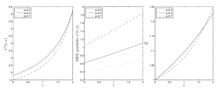
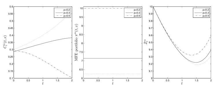
Figure 1: Top panel: The MFE consumption rate $C^{l}(t,x)$, the MFE portfolio $\pi^{l}(t,x)$, and the habit formation process $\bar{Z}^{l}_{t}$ with risk aversion parameters $p=0.2,~{}0.5$ and $0.7$. Bottom panel: The MFE consumption rate $C^{m}(t,x)$, the MFE portfolio $\pi^{m}(t,x)$, and the habit formation process $\bar{Z}^{m}_{t}$ with risk aversion parameters $p=0.2,~{}0.3$ and $0.5$.

In Figure 2, we numerically illustrate the impact by the habit formation intensity parameter $\delta$. We choose and fix $T=2,~{}p=0.1,~{}x_{0}=3,~{}z_{0}=0.5,~{}\mu=0.1,~{}\sigma=0.1,~{}x=2$ under the linear habit formation with different values $\delta=0.1,0.2,0.3$, and choose and fix $T=2,~{}p=0.4,~{}x_{0}=3,~{}z_{0}=10,~{}\mu=0.2,~{}\sigma=0.2,~{}x=1$ and $\alpha=1$ under the multiplicative habit formation with different values $\delta=0.1,0.2,0.3$. From the top panel, we observe that both the habit formation process $\bar{Z}^{l}_{t}$ and the MFE consumption rate $C^{l}(t,x)$ do not display simple monotonicity in the parameter $\delta$. These observations can be explained by the fact that the habit formation process of each agent is defined as the combination of the discounted initial value $z_{0}e^{-\delta t}$ (decreasing in $\delta$) and the weighted average $\int_{0}^{t}\delta e^{\delta(s-t)}C^{l}_{s}ds$ (usually increasing in $\delta$). When the initial level $z_{0}$ is very small, as plotted in the top-right panel, the average habit level $\bar{Z}^{l}_{t}$ depends on $\delta$ in a more subtle way. The addictive habit constraint then causes complicated dependence of $C^{l}(t,x)$ on the parameter $\delta$ as well. However, as illustrated in the bottom-right panel under the multiplicative habit formation, when the initial habit $z_{0}$ is very large, the term $z_{0}e^{-\delta t}$ significantly dominates the integral term $\int_{0}^{t}\delta e^{\delta(s-t)}C^{l}_{s}ds$, and hence the mean field average habit $\bar{Z}^{m}_{t}$ is observed as decreasing in $\delta$.

More importantly, we observe from the bottom-left panel of Figure 2 that the representative agent displays the hump-shaped consumption path, i.e. the consumption trajectory is first increasing in time and then decreasing in time, which matches with the well documented phenomenon in many empirical studies on individual’s consumption behavior. Kraft et al. (2017) has proposed and verified the internal habit formation preference as an effective answer to support the hump-shaped consumption pattern of the individual agent. From the perspective of mean field competition, we can also give an explanation to the hump-shaped equilibrium consumption when the initial habit is very high. At the beginning of the time horizon, the population’s average habit $\bar{Z}^{m}$ is high and decreasing in time $t$ due to the discount by $\delta$, and the competition mechanism takes the leading role in each agent’s decision making. That is, each agent would increase her consumption rate to attain higher excessive consumption and larger expected utility. As time moves on, the past increasing consumption path will take more effect in each agent’s habit formation process and the average habit level $\bar{Z}^{m}$ in the economy will also start to increase, indicating a high future standard of living in the society. As each agent has no obligation to consume above the high standard of living, the sense of competition is weakened and the self-satisfaction starts to take the leading role in decision making. Each agent is more likely to reduce her consumption rate after a period of time such that the growth rate of the population’s habit level can start to slow down and everyone may suffer less from the high future benchmark.

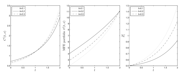
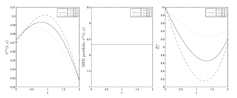
Figure 2: Top panel: The MFE consumption rate $C^{l}(t,x)$, the MFE portfolios $\pi^{l}(t,x)$, and the habit formation processes $\bar{Z}^{l}_{t}$ with habit persistence parameters $\delta=0.1,~{}0.2$ and $0.3$. Bottom panel: The MFE consumption rate $C^{m}(t,x)$, the MFE portfolios $\pi^{m}(t,x)$, and the habit formation processes $\bar{Z}^{m}_{t}$ with habit persistence parameters $\delta=0.1,~{}0.2$ and $0.3$.

At last, we illustrate in Figure 3 how the competition parameter $\alpha$ affects the MFE under the multiplicative habit formation. Let us fix model parameters $T=2,~{}p=0.5,~{}x_{0}=3,~{}\mu=0.1,~{}\delta=0.1,~{}\sigma=0.8,~{}x=1$ and consider different values $\alpha=0.5,~{}0.8,~{}1$. To compare with two previous figures, let us consider a small initial habit $z_{0}=0.2$ and illustrate the trend of $\bar{Z}^{m}_{t}$ and the MFE controls. As discussed previously, when the initial habit is low, the mean field habit formation process $\bar{Z}^{m}_{t}$ and the MFE consumption $C^{m}(t,x)$ become increasing functions of time $t$ that are similar to the case under the linear habit formation. In addition, we can see that both $\bar{Z}^{m}_{t}$ and $C^{m}(t,x)$ are increasing in the parameter $\alpha$, indicating that the more competitive the representative agent is, the higher equilibrium consumption policy she chooses and the average habit level of the population also gets larger.

Figure 3: The MFE consumption rate $C^{m}(t,x)$, the MFE portfolio $\pi^{m}(t,x)$, and the habit formation process $\bar{Z}^{m}_{t}$ with competition parameters $\alpha=0.5,~{}0.8$ and $1$.

5 Approximate Nash Equilibrium in n-player Games

This section examines the approximate Nash equilibrium in finite population games under two types of habit formation preferences when $n$ is sufficiently large. We will construct the approximate Nash equilibrium using the obtained mean field equilibrium from the previous section. Let us recall two previous assumptions $\bm{(A_{h})}$ and $\bm{(A_{o})}$. In this section, in order to derive the explicit convergence rate in terms of $n$, we need to further assume that the mean field model is symmetric:

• $\bm{(A_{c})}$: there exists a constant vector $o=(\mu,\sigma,p)\in\mathcal{O}$ such that $o_{n}\rightarrow o$ as $n\rightarrow\infty$ with the order of convergence $O(\frac{1}{\sqrt{n}})$.

Note that if the market model with $n$ agents is homogenous, i.e., the type vector $o_{i}=(\mu,\sigma,p)$ is symmetric for $i=1,\ldots,n$, the above assumption holds trivially.

5.1 Approximation under linear habit formation

For $i=1,\ldots,n$, we recall that the objective functional (2.5) of agent $i$ can be rewritten as: for $(\pi^{i},c^{i})\in{\cal A}^{l,i}(x_{0})$,

$$J^{l}_{i}((\pi^{i},c^{i}),(\bm{\pi},\bm{c})^{-i})=\mathbb{E}\left[\int_{0}^{T}U_{i}\left(c^{i}_{s}X_{s}^{i}-\bar{Z}_{s}^{n}\right)ds+U_{i}(X_{T}^{i})\right],$$ (5.1)

where the vector of policies $(\bm{\pi},\bm{c})^{-i}$ for $i=1,\ldots,n$ is defined by

$$(\bm{\pi},\bm{c})^{-i}:=((\pi^{1},c^{1}),\ldots,(\pi^{i-1},c^{i-1}),(\pi^{i+1},c^{i+1}),\ldots,(\pi^{n},c^{n})).$$ (5.2)

Then, the definition of an approximate Nash equilibrium for the model consisting of $n$ agents is defined as follows:

Definition 5.1 (Approximate Nash equilibrium).

Let ${\cal A}^{l}(x_{0}):=\prod_{i=1}^{n}{\cal A}^{l,i}(x_{0})$. An admissible strategy $(\bm{\pi}^{*,l},\bm{c}^{*,l})=((\pi^{*,l,1},c^{*,l,1}),\ldots,(\pi^{*,l,n},c^{*,l,n}))\in{\cal A}^{l}(x_{0})$ is called an $\epsilon$-Nash equilibrium to the $n$-player game problem (2.5) if, for any $((\pi^{i},c^{i}))_{i=1}^{n}\in{\cal A}^{l}(x_{0})$, it holds that

$$\sup_{(\pi^{i},c^{i})\in{\cal A}^{l,i}(x_{0})}J^{l}_{i}((\pi^{i},c^{i}),(\bm{\pi}^{*,l},\bm{c}^{*,l})^{-i})\leq J^{l}_{i}((\bm{\pi}^{*,l},\bm{c}^{*,l}))+\epsilon,\quad\forall i=1,\ldots,n.$$ (5.3)

In what follows, we plan to construct and verify the approximate Nash equilibrium for the $n$-player game. However, we note that the addictive habit constraint $C_{t}^{i}\geq\bar{Z}^{n}_{t}$, $t\in[0,T]$, needs to be guaranteed. Let us define $\overline{m}_{p}:=\sup_{i\in\mathbb{N}}p_{i}$ and $\underline{m}_{p}:=\inf_{i\in\mathbb{N}}p_{i}$. It is clear that $0<\underline{m}_{p}\leq\overline{m}_{p}<1$. For $i=1,\ldots,n$, we now give a careful construction of the candidate investment and consumption pair $(\pi^{*,l,i},c^{*,l,i})=(\pi_{t}^{*,l,i},c_{t}^{*,l,i})_{t\in[0,T]}$ for agent $i$ in the following form

$$\left\{\begin{aligned} &\pi_{t}^{*,l,i}:=\frac{\mu_{i}}{(1-p_{i})\sigma_{i}^{2}X_{t}^{*,l,i}}\left(X_{t}^{\bar{Z}^{l},i}-\int_{t}^{T}\bar{Z}^{l}_{s}ds\right),\\[3.99994pt] &c_{t}^{*,l,i}:=\frac{1}{X_{t}^{*,l,i}}\left(\bar{Z}_{t}^{*,l,n}+\left(X_{t}^{\bar{Z}^{l},i}-\int_{t}^{T}\bar{Z}^{l}_{s}ds\right)g^{l}_{i}(t)^{\frac{1}{p_{i}-1}}\right),\end{aligned}\right.$$ (5.4)

where $X^{*,l,i}=(X_{t}^{*,l,i})_{t\in[0,T]}$ is the wealth process defined in (2.2) for agent $i$ under the control $(\pi^{*,l,i},c^{*,l,i})$ that

$$\frac{dX_{t}^{*,l,i}}{X_{t}^{*,l,i}}=\pi_{t}^{*,l,i}\mu_{i}dt+\pi_{t}^{*,l,i}\sigma_{i}dW^{i}_{t}-c_{t}^{*,l,i}dt,\quad X_{0}^{*,l,i}=x_{0},$$ (5.5)

and the average habit formation process from $n$ agents is defined by $\bar{Z}_{t}^{*,l,n}:=\frac{1}{n}\sum_{i=1}^{n}Z_{t}^{*,l,i}$ with

$$Z_{t}^{*,l,i}=e^{-\delta t}\left(z_{0}+\int_{0}^{t}\delta e^{\delta s}c_{s}^{*,l,i}X_{s}^{*,l,i}ds\right).$$ (5.6)

The positive function $t\to g^{l}_{i}(t)$ is given by

$$g^{l}_{i}(t)=\left(\left(1+\frac{1}{a_{i}}\right)e^{a_{i}(T-t)}-\frac{1}{a_{i}}\right)^{1-p_{i}},\quad t\in[0,T],$$ (5.7)

with $a_{i}:=\frac{1}{2}\frac{\mu_{i}^{2}}{\sigma_{i}^{2}}\frac{p_{i}}{(1-p_{i})^{2}}>0$. Note that $\bar{Z}^{l}=(\bar{Z}^{l}_{t})_{t\in[0,T]}$ in (5.4) differs from the average habit formation process $\bar{Z}^{*,l,n}$ in the $n$-player game. Indeed, $\bar{Z}^{l}$ is the unique fixed point established in Proposition 3.1 in the mean field game problem, and the auxiliary process $X^{\bar{Z}^{l},i}=(X_{t}^{\bar{Z}^{l},i})_{t\in[0,T]}$ in (5.4) is defined by the SDE

$$\left\{\begin{aligned} \frac{d(X_{t}^{\bar{Z}^{l},i}-\int_{t}^{T}\bar{Z}^{l}_{s}ds)}{X_{t}^{\bar{Z}^{l},i}-\int_{t}^{T}\bar{Z}^{l}_{s}ds}&=\left(\frac{\mu_{i}^{2}}{(1-p_{i})\sigma_{i}^{2}}-g^{l}_{i}(t)^{\frac{1}{p_{i}-1}}\right)dt+\frac{\mu_{i}}{(1-p_{i})\sigma_{i}}dW^{i}_{t},\\ X_{0}^{\bar{Z}^{l},i}&=x_{0}.\end{aligned}\right.$$ (5.8)

It is clear that $(X_{t}^{\bar{Z}^{l},i}-\int_{t}^{T}\bar{Z}^{l}_{s}ds)_{t\in[0,T]}$ is a GBM for each $i$ that is nonnegative in view of Lemma 3.1. Moreover, we can write

$$X_{t}^{\bar{Z}^{l},i}-\int_{t}^{T}\bar{Z}_{s}^{l}ds=\left(x_{0}-\int_{0}^{T}\bar{Z}^{l}_{s}ds\right)\exp\left(\int_{0}^{t}G_{i}(s)ds+\frac{\mu_{i}}{(1-p_{i})\sigma_{i}}W^{i}_{t}\right)$$ (5.9)

with $G_{i}(t):=\frac{\mu_{i}^{2}}{(1-p_{i})\sigma_{i}^{2}}-g^{l}_{i}(t)^{\frac{1}{p_{i}-1}}-\frac{\mu_{i}^{2}}{2(1-p_{i})^{2}\sigma_{i}^{2}}$ for all $t\in[0,T]$. As $X_{t}^{\bar{Z}^{l},i}>\int_{t}^{T}\bar{Z}_{s}^{l}ds$ and $g_{i}^{l}(t)>0$ for $t\in[0,T]$, by definition in (5.4), it is clear that the addictive habit constraint $C_{t}^{*,l,i}=c_{t}^{*,l,j}X_{t}^{*,l,i}>\bar{Z}_{t}^{*,l,n}$, $t\in[0,T]$, is satisfied. In fact, we can show in the next result that $C^{*,l,i}$ can be fully expressed by the given $\bar{Z}^{l}$. Let us denote the average aggregate consumption rate

$$\bar{C}_{t}^{*,l,n}:=\frac{1}{n}\sum_{i=1}^{n}C_{t}^{*,l,i}=\frac{1}{n}\sum_{i=1}^{n}c_{t}^{*,l,i}X_{t}^{*,l,i}.$$ (5.10)

We also recall that $d\bar{Z}_{t}^{*,l,n}=-\delta(\bar{Z}_{t}^{*,l,n}-\bar{C}_{t}^{*,l,n})dt$.

Lemma 5.1.

Let $\bar{Z}^{l}=(\bar{Z}_{t}^{l})_{t\in[0,T]}\in{\cal C}_{T,x_{0}}$ be the unique fixed point in Proposition 3.1. Then, we can express the average consumption rate $\bar{C}_{t}^{*,l,n}$ and the average habit formation process $\bar{Z}_{t}^{*,l,n}$ explicitly in terms of $\bar{Z}^{l}$ that

$$\begin{cases}\displaystyle\bar{C}_{t}^{*,l,n}=\bar{Z}_{t}^{*,l,n}+\left(x_{0}-\int_{0}^{T}\bar{Z}^{l}_{s}ds\right)\frac{1}{n}\sum_{i=1}^{n}\exp\left(\int_{0}^{t}G_{i}(s)ds+\frac{\mu_{i}}{(1-p_{i})\sigma_{i}}W^{i}_{t}\right)g_{i}(t)^{\frac{1}{p_{i}-1}},\\[16.00008pt] \displaystyle\bar{Z}_{t}^{*,l,n}=z_{0}+\left(x_{0}-\int_{0}^{T}\bar{Z}^{l}_{s}ds\right)\int_{0}^{t}\frac{\delta}{n}\sum_{i=1}^{n}\exp\left(\int_{0}^{s}G_{i}(v)dv+\frac{\mu_{i}}{(1-p_{i})\sigma_{i}}W^{i}_{s}\right)ds.\end{cases}$$ (5.11)

Moreover, for any $q\geq 1$, it holds that $\sup_{t\in[0,T]}\mathbb{E}[(\bar{Z}_{t}^{*,l,n})^{q}]\leq C_{q,T}$ for some constant $C_{q,T}>0$ that is independent of $n$.

Proof.

In view of (5.4) and (5.10), we have that

$$\bar{C}_{t}^{*,l,n} =\bar{Z}_{t}^{*,l,n}+\frac{1}{n}\sum_{i=1}^{n}\left(X_{t}^{\bar{Z}^{l},i}-\int_{t}^{T}\bar{Z}^{l}_{s}ds\right)g^{l}_{i}(t)^{\frac{1}{p_{i}-1}}.$$ (5.12)

Then, it holds from (5.12) that

$$d\bar{Z}_{t}^{*,l,n} =-\delta(\bar{Z}_{t}^{*,l,n}-\bar{C}_{t}^{*,l,n})dt=\frac{\delta}{n}\sum_{i=1}^{n}\left(X_{t}^{\bar{Z}^{l},i}-\int_{t}^{T}\bar{Z}^{l}_{s}ds\right)g^{l}_{i}(t)^{\frac{1}{p_{i}-1}}.$$

The equalities in (5.11) follow directly from (5.9). By using the second equality in (5.11), it follows from Jensen’s inequality that

$$\sup_{t\in[0,T]}\mathbb{E}\left[\left(\bar{Z}_{t}^{*,l,n}\right)^{q}\right]$$

$$\quad=\sup_{t\in[0,T]}\mathbb{E}\left[\left(z_{0}+\left(x_{0}-\int_{0}^{T}\bar{Z}^{l}_{s}ds\right)\int_{0}^{t}\frac{\delta}{n}\sum_{i=1}^{n}\exp\left(\int_{0}^{s}G_{i}(v)dv+\frac{\mu_{i}}{(1-p_{i})\sigma_{i}}W^{i}_{s}\right)ds\right)^{q}\right]$$

$$\quad\leq C_{q}z_{0}^{q}+C_{q,T}\left(x_{0}-\int_{0}^{T}\bar{Z}^{l}_{s}ds\right)^{q}\int_{0}^{T}\frac{1}{n}\sum_{i=1}^{n}\mathbb{E}\left[\exp\left(\int_{0}^{s}qG_{i}(v)dv+\frac{q\mu_{i}}{(1-p_{i})\sigma_{i}}W^{i}_{s}\right)\right]ds$$

$$\quad=C_{q}z_{0}^{q}+C_{q,T}\left(x_{0}-\int_{0}^{T}\bar{Z}^{l}_{s}ds\right)^{q}\int_{0}^{T}\frac{1}{n}\sum_{i=1}^{n}\exp\left(\int_{0}^{s}qG_{i}(v)dv+\frac{q^{2}\mu_{i}^{2}}{2(1-p_{i})^{2}\sigma_{i}^{2}}s\right)ds.$$

Then, the desired estimate on $\sup_{t\in[0,T]}\mathbb{E}[(\bar{Z}_{t}^{*,l,n})^{q}]$ follows from the assumption $\bm{(A_{c})}$. Thus, we complete the proof of the lemma. ∎

We now present the main result of this subsection on the existence of an approximate Nash equilibrium under linear external habit formation.

Theorem 5.1.

The control pair $(\bm{\pi}^{\ast,l},\bm{c}^{\ast,l})=((\pi^{*,l,1},c_{t}^{*,l,1}),\ldots,(\pi^{*,l,n},c_{t}^{*,l,n}))_{t\in[0,T]}$ given in (5.4) is an $\epsilon_{n}$-Nash equilibrium for the $n$-player game problem (2.5) with the explicit order $\epsilon_{n}=O(n^{-\frac{\underline{m}_{p}}{2}})$.

To prove Theorem 5.1, we need the following auxiliary results. First, a direct implication of the representation (5.9) is given in the next lemma, whose proof is omitted.

Lemma 5.2.

Let $\bar{Z}^{l}=(\bar{Z}_{t}^{l})_{t\in[0,T]}\in{\cal C}_{T,x_{0}}$ be the unique fixed point in Proposition 3.1. Then, for any $q>0$, there exists a constant $C_{q}>0$ independent of $i$ such that

$$\sup_{t\in[0,T]}\mathbb{E}\left[\left(X_{t}^{\bar{Z}^{l},i}-\int_{t}^{T}\bar{Z}_{s}^{l}ds\right)^{q}\right]\leq C_{q}.$$ (5.13)

The next result follows from Lemmas 5.2 and 5.1.

Lemma 5.3.

For $q\geq 1$, there exists a $C_{q}>0$ independent of $i$ such that $\sup_{t\in[0,T]}\mathbb{E}[(Z_{t}^{*,l,i})^{q}]\leq C_{q}$. Moreover, it holds that

$$\sup_{t\in[0,T]}\mathbb{E}\left[\left|\bar{Z}_{t}^{*,l,n}-\bar{Z}^{l}_{t}\right|^{2}\right]=O\left(n^{-1}\right).$$ (5.14)

Proof.

We have that

$$\bar{Z}_{t}^{*,l,n}-\bar{Z}^{l}_{t}=e^{-\delta t}\int_{0}^{t}\delta e^{\delta s}\left(\frac{1}{n}\sum_{i=1}^{n}c_{s}^{*,l,i}X_{s}^{*,l,i}-\mathbb{E}[c_{s}^{l}X_{s}^{l,\bar{Z}^{l}}]\right)ds$$

$$\quad=e^{-\delta t}\int_{0}^{t}\delta e^{\delta s}\left\{\frac{1}{n}\sum_{i=1}^{n}\left(\bar{Z}_{s}^{*,l,n}+\left(X_{s}^{\bar{Z}^{l},i}-\int_{s}^{T}\bar{Z}^{l}_{u}du\right)g^{l}_{i}(s)^{\frac{1}{p_{i}-1}}\right)\right.$$

$$\quad\qquad\left.-\bar{Z}^{l}_{s}-\mathbb{E}\left[\left(X_{s}^{l,\bar{Z}^{l}}-\int_{s}^{T}\bar{Z}_{u}^{l}du\right)g^{l}(s)^{\frac{1}{p-1}}\right]\right\}ds$$

$$\quad=\int_{0}^{t}\delta e^{\delta(s-t)}\left(\bar{Z}_{s}^{*,l,n}-\bar{Z}^{l}_{s}\right)ds+\int_{0}^{t}\delta e^{\delta(s-t)}\left[\frac{1}{n}\sum_{i=1}^{n}X_{s}^{\bar{Z}^{l},i}-\mathbb{E}\left[X_{s}^{l,\bar{Z}^{l}}\right]\right]g^{l}(s)^{\frac{1}{p-1}}ds$$

$$\qquad\quad+\int_{0}^{t}\delta e^{\delta(s-t)}\left[\frac{1}{n}\sum_{i=1}^{n}\left(X_{s}^{\bar{Z}^{l},i}-\int_{s}^{T}\bar{Z}^{l}_{u}du\right)\left(g^{l}_{i}(s)^{\frac{1}{p_{i}-1}}-g^{l}(s)^{\frac{1}{p-1}}\right)\right]ds.$$

Then, by applying Cauchy inequality, it holds that

$$\left|\bar{Z}_{t}^{*,l,n}-\bar{Z}^{l}_{t}\right|^{2} \leq 4\left(\int_{0}^{t}\delta\left|\bar{Z}_{s}^{*,l,n}-\bar{Z}^{l}_{s}\right|ds\right)^{2}+4\left(\int_{0}^{t}\delta\left|\frac{1}{n}\sum_{i=1}^{n}X_{s}^{\bar{Z}^{l},i}-\mathbb{E}\left[X_{s}^{l,\bar{Z}^{l}}\right]\right|ds\right)^{2}$$

$$\quad+4\left(\int_{0}^{t}\delta e^{\delta(s-t)}\frac{1}{n}\sum_{i=1}^{n}\left|g^{l}_{i}(s)^{\frac{1}{p_{i}-1}}-g^{l}(s)^{\frac{1}{p-1}}\right|\left(X_{s}^{\bar{Z}^{l},i}-\int_{s}^{T}\bar{Z}^{l}_{u}du\right)ds\right)^{2}$$

$$\leq 4\delta^{2}T\int_{0}^{t}\left|\bar{Z}_{s}^{*,l,n}-\bar{Z}^{l}_{s}\right|^{2}ds+4\delta^{2}T\int_{0}^{t}\left|\frac{1}{n}\sum_{i=1}^{n}X_{s}^{\bar{Z}^{l},i}-\mathbb{E}\left[X_{s}^{l,\bar{Z}^{l}}\right]\right|^{2}ds$$

$$\quad+4\delta^{2}T\int_{0}^{t}\left(\frac{1}{n}\sum_{i=1}^{n}\left|g^{l}_{i}(s)^{\frac{1}{p_{i}-1}}-g^{l}(s)^{\frac{1}{p-1}}\right|\left(X_{s}^{\bar{Z}^{l},i}-\int_{s}^{T}\bar{Z}^{l}_{u}du\right)\right)^{2}ds.$$

There exists a constant $C_{T}>0$ depending on $T$ only, but it may be different from line to line that

$$\mathbb{E}\left[\left|\bar{Z}_{t}^{*,l,n}-\bar{Z}^{l}_{t}\right|^{2}\right]$$

$$\qquad\leq C_{T}\int_{0}^{t}\mathbb{E}\left[\left|\bar{Z}_{s}^{*,l,n}-\bar{Z}^{l}_{s}\right|^{2}\right]ds+C_{T}\int_{0}^{t}\mathbb{E}\left[\left|\frac{1}{n}\sum_{i=1}^{n}X_{s}^{\bar{Z}^{l},i}-\mathbb{E}\left[X_{s}^{l,\bar{Z}^{l}}\right]\right|^{2}\right]ds$$

$$\qquad\quad+C_{T}\int_{0}^{t}\left(\frac{1}{n}\sum_{i=1}^{n}\left(g^{l}_{i}(s)^{\frac{1}{p_{i}-1}}-g^{l}(s)^{\frac{1}{p-1}}\right)^{2}\right)\mathbb{E}\left[\frac{1}{n}\sum_{i=1}^{n}\left(X_{s}^{\bar{Z}^{l},i}-\int_{s}^{T}\bar{Z}^{l}_{u}du\right)\right]ds$$

$$\qquad\leq C_{T}\int_{0}^{t}\mathbb{E}\left[\left|\frac{1}{n}\sum_{i=1}^{n}X_{s}^{\bar{Z}^{l},i}-\mathbb{E}\left[X_{s}^{l,\bar{Z}^{l}}\right]\right|^{2}\right]ds$$

$$\qquad\quad+C_{T}\int_{0}^{t}\frac{1}{n}\sum_{i=1}^{n}\left(g^{l}_{i}(s)^{\frac{1}{p_{i}-1}}-g^{l}(s)^{\frac{1}{p-1}}\right)^{2}ds+C_{T}\int_{0}^{t}\mathbb{E}\left[\left|\bar{Z}_{s}^{*,l,n}-\bar{Z}^{l}_{s}\right|^{2}\right]ds$$

$$\qquad:=L_{1}^{(n)}+L_{2}^{(n)}(t)+C_{T}\int_{0}^{t}\mathbb{E}\left[\left|\bar{Z}_{s}^{*,l,n}-\bar{Z}^{l}_{s}\right|^{2}\right]ds.$$ (5.15)

For the estimate of $L_{1}^{(n)}(t)$, we introduce the following SDE, for $i=1,\ldots,n$,

$$\frac{d\tilde{X}_{t}^{i}}{\tilde{X}_{t}^{i}}=\pi^{l}(t,\tilde{X}_{t}^{i})\mu dt+\pi^{l}(t,\tilde{X}_{t}^{i})\sigma dW_{t}^{i}-c^{l}(t,\tilde{X}_{t}^{i})dt,\quad\tilde{X}_{0}^{i}=x_{0},$$ (5.16)

where $\pi^{l}(t,x)=\pi^{*,\bar{Z}^{l}}(t,x)$ and $c^{l}(t,x)=c^{*,\bar{Z}^{l}}(t,x)$ are defined in (3.8) as the (feedback) mean field equilibrium with the given $\bar{Z}^{l}$. Hence, $(\tilde{X}^{i})_{i=1}^{n}$ are i.i.d. such that $\mathbb{E}[\tilde{X}_{t}^{i}]=\mathbb{E}[X_{t}^{l,\bar{Z}^{l}}]$ for all $i=1,\ldots,n$. Here, we recall that $X^{l,\bar{Z}^{l}}=(X_{t}^{l,\bar{Z}^{l}})_{t\in[0,T]}$ satisfies the dynamics

$$\frac{dX_{t}^{l,\bar{Z}^{l}}}{X_{t}^{l,\bar{Z}^{l}}}=\pi^{l}(t,X_{t}^{l,\bar{Z}^{l}})\mu dt+\pi^{l}(t,X_{t}^{l,\bar{Z}^{l}})\sigma dW_{t}-c^{l}(t,X_{t}^{l,\bar{Z}^{l}})dt,\quad X_{0}^{l,\bar{Z}^{l}}=x_{0}.$$ (5.17)

It follows from Jensen’s inequality that

$$\mathbb{E}\left[\left|\frac{1}{n}\sum_{i=1}^{n}X_{t}^{\bar{Z}^{l},i}-\mathbb{E}[X_{t}^{l,\bar{Z}^{l}}]\right|^{2}\right] \leq 2\mathbb{E}\left[\left|\frac{1}{n}\sum_{i=1}^{n}X_{t}^{\bar{Z}^{l},i}-\frac{1}{n}\sum_{i=1}^{n}\tilde{X}_{t}^{i}\right|^{2}\right]+2\mathbb{E}\left[\left|\frac{1}{n}\sum_{i=1}^{n}\tilde{X}_{t}^{i}-\mathbb{E}[X_{t}^{l,\bar{Z}^{l}}]\right|^{2}\right]$$

$$\leq\frac{2}{n}\sum_{i=1}^{n}\mathbb{E}\left[\left|X_{t}^{\bar{Z}^{l},i}-\tilde{X}_{t}^{i}\right|^{2}\right]+\frac{2}{n^{2}}\mathbb{E}\left[\left|\sum_{i=1}^{n}(\tilde{X}_{t}^{i}-\mathbb{E}[X_{t}^{l,\bar{Z}^{l}}])\right|^{2}\right]$$

$$=\frac{2}{n}\sum_{i=1}^{n}\mathbb{E}\left[\left|X_{t}^{\bar{Z}^{l},i}-\tilde{X}_{t}^{i}\right|^{2}\right]+\frac{2}{n^{2}}\sum_{i=1}^{n}\mathbb{E}\left[\left|\tilde{X}_{t}^{i}-\mathbb{E}[X_{t}^{l,\bar{Z}^{l}}]\right|^{2}\right]$$

$$=\frac{2}{n}\sum_{i=1}^{n}\mathbb{E}\left[\left|X_{t}^{\bar{Z}^{l},i}-\tilde{X}_{t}^{i}\right|^{2}\right]+\frac{2}{n}\mathbb{E}\left[\left|\tilde{X}_{t}^{1}-\mathbb{E}[X_{t}^{l,\bar{Z}^{l}}]\right|^{2}\right].$$ (5.18)

Denote by $\theta_{i}:=\frac{\mu_{i}}{(1-p_{i})\sigma_{i}^{2}}$ and $\theta:=\frac{\mu}{(1-p)\sigma^{2}}$. We deduce from (5.8) and (5.16) that

$$X_{t}^{\bar{Z}^{l},i}-\tilde{X}_{t}^{i}$$

$$=\int_{0}^{t}\left[\left(\mu_{i}\theta_{i}-g^{l}_{i}(s)^{\frac{1}{p_{i}-1}}\right)\left(X_{s}^{\bar{Z}^{l},i}-\tilde{X}_{s}^{i}\right)+\left(\mu_{i}\theta_{i}-g^{l}_{i}(s)^{\frac{1}{p_{i}-1}}-\mu\theta+g^{l}(s)^{\frac{1}{p-1}}\right)\left(\tilde{X}_{s}^{i}-\int_{s}^{T}\bar{Z}^{l}_{s}ds\right)\right]ds$$

$$\quad+\int_{0}^{t}\left[\sigma_{i}\theta_{i}\left(X_{s}^{\bar{Z}^{l},i}-\tilde{X}_{s}^{i}\right)+\left(\sigma_{i}\theta_{i}-\sigma\theta\right)\left(\tilde{X}_{s}^{i}-\int_{s}^{T}\bar{Z}^{l}_{s}ds\right)\right]dW_{s}^{i}.$$

In the sequel, let $C_{T}>0$ be a generic constant depending on $T$ only, which may be different from line to line. By applying Lemma 5.2 and BDG inequality, we deduce that

$$\mathbb{E}\left[\left|X_{t}^{\bar{Z}^{l},i}-\tilde{X}_{t}^{i}\right|^{2}\right] \leq C_{T}\int_{0}^{t}\mathbb{E}\left[\left|X_{s}^{\bar{Z}^{l},i}-\tilde{X}_{s}^{i}\right|^{2}\right]ds+C_{T}\int_{0}^{t}\left|\mu_{i}\theta_{i}-g^{l}_{i}(s)^{\frac{1}{p_{i}-1}}-\mu\theta+g^{l}(s)^{\frac{1}{p-1}}\right|^{2}ds$$

$$\quad+C_{T}\left(\sigma_{i}\theta_{i}-\sigma\theta\right)^{2}+C_{T}\int_{0}^{t}\mathbb{E}\left[\left|X_{s}^{\bar{Z}^{l},i}-\tilde{X}_{s}^{i}\right|^{2}\right]ds$$

$$\leq C_{T}\int_{0}^{t}\mathbb{E}\left[\left|X_{s}^{\bar{Z}^{l},i}-\tilde{X}_{s}^{i}\right|^{2}\right]ds+C_{T}\int_{0}^{t}\left|\mu_{i}\theta_{i}-g^{l}_{i}(s)^{\frac{1}{p_{i}-1}}-\mu\theta+g^{l}(s)^{\frac{1}{p-1}}\right|^{2}ds$$

$$\quad+C_{T}(\sigma_{i}\theta_{i}-\sigma\theta)^{2}.$$

Thus, we arrive from (5.4) at

$$\frac{1}{n}\sum_{i=1}^{n}\mathbb{E}\left[\left|X_{t}^{\bar{Z}^{l},i}-\tilde{X}_{t}^{i}\right|^{2}\right] \leq C_{T}\int_{0}^{t}\frac{1}{n}\sum_{i=1}^{n}\mathbb{E}\left[\left|X_{s}^{\bar{Z}^{l},i}-\tilde{X}_{s}^{i}\right|^{2}\right]ds+\frac{C_{T}}{n}\sum_{i=1}^{n}\left|\sigma_{i}\theta_{i}-\sigma\theta\right|^{2}$$

$$\quad+C_{T}\int_{0}^{t}\frac{1}{n}\sum_{i=1}^{n}\left|\mu_{i}\theta_{i}-g^{l}_{i}(s)^{\frac{1}{p_{i}-1}}-\mu\theta+g^{l}(s)^{\frac{1}{p-1}}\right|^{2}ds.$$ (5.19)

It follows from the assumption $\bm{(A_{c})}$ that

$$\begin{cases}\displaystyle\frac{1}{n}\sum_{i=1}^{n}\left|\sigma_{i}\theta_{i}-\sigma\theta\right|^{2}=O\left(n^{-1}\right),\\ \displaystyle\sup_{s\in[0,T]}\frac{1}{n}\sum_{i=1}^{n}\left|\mu_{i}\theta_{i}-g^{l}_{i}(s)^{\frac{1}{p_{i}-1}}-\mu\theta+g^{l}(s)^{\frac{1}{p-1}}\right|^{2}=O\left(n^{-1}\right).\end{cases}$$ (5.20)

Then, the Gronwall’s lemma with (5.1) yields that

$$\sup_{t\in[0,T]}\frac{1}{n}\sum_{i=1}^{n}\mathbb{E}\left[\left|X_{t}^{\bar{Z}^{l},i}-\tilde{X}_{t}^{i}\right|^{2}\right]=O\left(n^{-1}\right).$$ (5.21)

Moreover, we also have from (5.20) that $L_{2}^{(n)}(t)=O(n^{-1})$. Finally, it is obvious to have that

$$\frac{2}{n}\sup_{t\in[0,T]}\mathbb{E}\left[\left|\tilde{X}_{t}^{1}-\mathbb{E}[X_{t}^{l,\bar{Z}^{l}}]\right|^{2}\right]=O\left(n^{-1}\right).$$ (5.22)

Therefore, by (5.1) and (5.22), it holds that $L_{1}^{(n)}(t)=O(n^{-1})$. Then, applying Gronwall’s inequality to (5.1) yields (5.14). ∎

We then provide the proof of Theorem 5.1.

Proof of Theorem 5.1.

For $i=1,\ldots,n$, let $Z^{i}=(Z_{t}^{i})_{t\in[0,T]}$ and $Z^{*,l,i}=(Z_{t}^{*,l,i})_{t\in[0,T]}$ be the habit formation processes of agent $i$ under an arbitrary admissible strategy $(\pi^{i},c^{i})\in{\cal A}^{l,i}(x_{0})$ and under the strategy $(\pi^{*,l,i},c^{*,l,i})\in{\cal A}^{l,i}(x_{0})$ given in (5.4) respectively. We denote

$$\bar{Z}^{*,l,n,-i}_{t}:=\frac{1}{n}\sum_{j\neq i}Z_{t}^{\ast,l,j},\quad t\in[0,T].$$ (5.23)

In terms of (2.5), we have that, for $i=1,\ldots,n$,

$$J^{l}_{i}((\pi^{i},c^{i}),(\bm{\pi}^{*,l},\bm{c}^{*,l})^{-i}) =\mathbb{E}\left[\int_{0}^{T}U_{i}\left(c^{i}_{s}X_{s}^{i}-\bar{Z}_{s}^{*,l,n,-i}-\frac{1}{n}Z_{s}^{i}\right)ds+U_{i}(X_{T}^{i})\right],$$

$$J^{l}_{i}((\pi^{*,l,i},c^{*,l,i}),(\bm{\pi}^{*,l},\bm{c}^{*,l})^{-i}) =\mathbb{E}\left[\int_{0}^{T}U_{i}\left(c^{*,l,i}_{s}X_{s}^{*,l,i}-\bar{Z}_{s}^{*,l,n}\right)ds+U_{i}(X_{T}^{*,l,i})\right].$$

where $X^{*,l,i}=(X_{t}^{*,l,i})_{t\in[0,T]}$ obeys the dynamics (5.5), and for an admissible control $(\pi^{i},c^{i})\in{\cal A}^{l,i}(x_{0})$, the process $X^{i}=(X_{t}^{i})_{t\in[0,T]}$ satisfies

$$\frac{dX_{t}^{i}}{X_{t}^{i}}=\pi^{i}_{t}\mu_{i}dt+\pi^{i}_{t}\sigma_{i}dW^{i}_{t}-c^{i}_{t}dt,\quad X_{0}^{i}=x_{0}.$$ (5.24)

In order to prove (5.37) in Definition 5.2, we also introduce an auxiliary optimal control problem (P): for $\bar{Z}^{l}=(\bar{Z}^{l}_{t})_{t\in[0,T]}$ being the unique fixed point in Proposition 3.1, let us consider

$$\sup_{(\pi^{i},c^{i})\in\mathcal{A}^{l,i}(x_{0})}\bar{J}_{i}((\pi^{i},c^{i});\bar{Z}^{l}):=\sup_{(\pi^{i},c^{i})\in\mathcal{A}^{l,i}(x_{0})}\mathbb{E}\left[\int_{0}^{T}U_{i}\left(c^{i}_{s}{X}_{s}^{i}-\bar{Z}^{l}_{s}\right)ds+U_{i}({X}_{T}^{i})\right],$$ (5.25)

It is straightforward to see that the optimal strategy of the auxiliary control problem (P) is

$$\left\{\begin{aligned} &\pi_{t}^{*,\bar{Z}^{l},i}=\frac{\mu_{i}}{(1-p_{i})\sigma_{i}^{2}X_{t}^{\bar{Z}^{l},i}}\left(X_{t}^{\bar{Z}^{l},i}-\int_{t}^{T}\bar{Z}^{l}_{s}ds\right),\\[3.99994pt] &c_{t}^{*,\bar{Z}^{l},i}=\frac{1}{X_{t}^{\bar{Z}^{l},i}}\left(\bar{Z}^{l}_{t}+\left(X_{t}^{\bar{Z}^{l},i}-\int_{t}^{T}\bar{Z}^{l}_{s}ds\right)g^{l}_{i}(t)^{\frac{1}{p_{i}-1}}\right),\end{aligned}\right.$$ (5.26)

where the controlled wealth process $X^{\bar{Z}^{l},i}=(X^{\bar{Z}^{l},i}_{t})_{t\in[0,T]}$ is given by (5.9).

We then focus on the verification of (5.37) by using the auxiliary problem $(\bf{P})$ in (5.25). We have that

$$\sup_{(\pi^{i},c^{i})\in\mathcal{A}^{l,i}(x_{0})}J^{l}_{i}\left((\pi^{i},c^{i}),(\bm{\pi}^{*,l},\bm{c}^{*,l})^{-i}\right)-J^{l}_{i}\left(\bm{\pi}^{*,l},\bm{c}^{*,l}\right)$$

$$\qquad=\left(\sup_{(\pi^{i},c^{i})\in\mathcal{A}^{l,i}(x_{0})}J^{l}_{i}\left((\pi^{i},c^{i}),(\bm{\pi}^{*,l},\bm{c}^{*,l})^{-i}\right)-\sup_{(\pi^{i},c^{i})\in\mathcal{A}^{l}(x_{0})}\bar{J}^{l}_{i}\left((\pi^{i},c^{i});\bar{Z}^{l}\right)\right)$$

$$\qquad\quad+\sup_{(\pi^{i},c^{i})\in\mathcal{A}^{l,i}(x_{0})}\bar{J}^{l}_{i}\left((\pi^{i},c^{i});\bar{Z}^{l}\right)-J_{i}^{l}\left(\bm{\pi}^{*,l},\bm{c}^{*,l}\right)$$

$$\qquad\leq\sup_{(\pi^{i},c^{i})\in\mathcal{A}^{l,i}(x_{0})}\left(J_{i}^{l}\left((\pi^{i},c^{i}),(\bm{\pi}^{*,l},\bm{c}^{*,l})^{-i}\right)-\bar{J}^{l}_{i}\left((\pi^{i},c^{i});\bar{Z}^{l}\right)\right)$$

$$\qquad\quad+\sup_{(\pi^{i},c^{i})\in\mathcal{A}^{l,i}(x_{0})}\bar{J}^{l}_{i}\left((\pi^{i},c^{i});\bar{Z}^{l}\right)-J^{l}_{i}\left(\bm{\pi}^{*,l},\bm{c}^{*,l}\right).$$ (5.27)

We first evaluate the first term of RHS of (5.1) that, for all $(\pi^{i},c^{i})\in\mathcal{A}^{l,i}(x_{0})$,

$$J^{l}_{i}((\pi^{i},c^{i}),(\bm{\pi}^{*,l,i},\bm{c}^{*,l,i})^{-i})-\bar{J}^{l}_{i}((\pi^{i},c^{i});\bar{Z}^{l})$$

$$\quad=\left\{\mathbb{E}\left[\int_{0}^{T}U_{i}\left(c^{i}_{s}X_{s}^{i}-\bar{Z}_{s}^{*,l,n,-i}-\frac{1}{n}Z_{s}^{i}\right)ds\right]-\mathbb{E}\left[\int_{0}^{T}U_{i}\left(c^{i}_{s}X_{s}^{i}-\bar{Z}_{s}^{*,l,n}\right)ds\right]\right\}$$

$$\qquad+\left\{\mathbb{E}\left[\int_{0}^{T}U_{i}\left(c^{i}_{s}X_{s}^{i}-\bar{Z}_{s}^{*,l,n}\right)ds\right]-\mathbb{E}\left[\int_{0}^{T}U_{i}\left(c^{i}_{s}X_{s}^{i}-\bar{Z}^{l}_{s}\right)ds\right]\right\}$$

$$\quad:=I_{i}^{(1)}+I_{i}^{(2)}.$$

For the term $I_{i}^{(1)}$, we have that

$$I_{i}^{(1)}=\frac{1}{p_{i}}\mathbb{E}\left[\int_{0}^{T}\left[\left(c^{i}_{s}X_{s}^{i}-\bar{Z}_{s}^{*,l,n,-i}-\frac{1}{n}Z_{s}^{i}\right)^{p_{i}}-\left(c^{i}_{s}X_{s}^{i}-\bar{Z}_{s}^{*,l,n}\right)^{p_{i}}\right]ds\right].$$

Using the inequality $(a+b)^{p_{i}}\leq a^{p_{i}}+b^{p_{i}}$ for all $a,b>0$, we can derive on the event $\{Z_{s}^{*,l,i}>Z_{s}^{i}\}$ that

$$\left(c^{i}_{s}X_{s}^{i}-\bar{Z}_{s}^{*,l,n,-i}-\frac{1}{n}Z_{s}^{i}\right)^{p_{i}}-\left(c^{i}_{s}X_{s}^{i}-\bar{Z}_{s}^{*,l,n}\right)^{p_{i}}\leq\left(\bar{Z}_{s}^{*,l,n}-\bar{Z}_{s}^{*,l,n,-i}-\frac{1}{n}Z_{s}^{i}\right)^{p_{i}}$$

$$= \frac{1}{n^{p_{i}}}\left(Z_{s}^{\ast,l,i}-Z_{s}^{i}\right)^{p_{i}}\leq\frac{1}{n^{p_{i}}}\left(Z_{s}^{\ast,l,i}\right)^{p_{i}}.$$ (5.28)

With the help of Lemma 5.3, the Jensen inequality with (5.1) and $p_{i}\in(0,1)$, we arrive at

$$I_{i}^{(1)} \leq\frac{1}{p_{i}}\mathbb{E}\left[\int_{0}^{T}\frac{1}{n^{p_{i}}}\left(Z_{s}^{\ast,l,i}\right)^{p_{i}}ds\right]\leq\frac{1}{p_{i}}\frac{1}{n^{p_{i}}}\int_{0}^{T}\left(\mathbb{E}\left[Z_{s}^{\ast,l,i}\right]\right)^{p_{i}}dt\leq\frac{C_{T}}{n^{p_{i}}}=O(n^{-\underline{m}_{p}}),$$

for some constant $C_{T}>0$ independent of $i$. Here, we have used the fact that $0<\underline{m}_{p}:=\inf_{i\in\mathbb{N}}p_{i}\leq\bar{m}_{p}:=\sup_{i\in\mathbb{N}}p_{i}<1$. On the other hand, on the event $\{Z_{s}^{*,l,i}\leq Z_{s}^{i}\}$, we have that $(c^{i}_{s}X_{s}^{i}-\bar{Z}_{s}^{*,l,n,-i}-\frac{1}{n}Z_{s}^{i})^{p_{i}}-(c^{i}_{s}X_{s}^{i}-\bar{Z}_{s}^{*,l,n})^{p_{i}}\leq 0$. This yields that

$$I_{i}^{(1)} =\frac{1}{p_{i}}\mathbb{E}\left[\int_{0}^{T}\left[\left(c^{i}_{s}X_{s}^{i}-\bar{Z}_{s}^{*,l,n,-i}-\frac{1}{n}Z_{s}^{i}\right)^{p_{i}}-\left(c^{i}_{s}X_{s}^{i}-\bar{Z}_{s}^{*,l,n}\right)^{p_{i}}\right]ds\right]=O(n^{-\underline{m}_{p}}).$$ (5.29)

Similarly, for the term $I_{i}^{(2)}$, it suffices to consider its estimate on the event $\{\bar{Z}^{l}_{s}>\bar{Z}_{s}^{*,l,n}\}$, on which we have

$$(c^{i}_{s}X_{s}^{i}-\bar{Z}_{s}^{*,l,n})^{p_{i}}-(c^{i}_{s}X_{s}^{i}-\bar{Z}^{l}_{s})^{p_{i}} \leq(\bar{Z}_{s}^{l}-\bar{Z}_{s}^{\ast,l,n})^{p_{i}}.$$

By applying Hölder inequality and Lemma 5.3, it holds that

$$I_{i}^{(2)} =\mathbb{E}\left[\int_{0}^{T}\left[\left(c^{i}_{s}X_{s}^{i}-\bar{Z}_{s}^{*,l,n}\right)^{p_{i}}-\left(c^{i}_{s}X_{s}^{i}-\bar{Z}^{l}_{s}\right)^{p_{i}}\right]ds\right]\leq\frac{1}{p_{i}}\mathbb{E}\left[\int_{0}^{T}\left(\bar{Z}^{l}_{s}-\bar{Z}_{s}^{*,l,n}\right)^{p_{i}}ds\right]$$

$$\leq\frac{1}{p_{i}}\int_{0}^{T}\mathbb{E}\left[\left|\bar{Z}^{l}_{s}-\bar{Z}_{s}^{*,l,n}\right|^{2}\right]^{\frac{p_{i}}{2}}ds=O\left(n^{-\frac{\underline{m}_{p}}{2}}\right).$$ (5.30)

We then conclude that

$$\sup_{(\pi^{i},c^{i})\in\mathcal{A}^{l,i}(x_{0})}\left(J^{l}_{i}\left((\pi^{i},c^{i}),(\bm{\pi}^{*,l},\bm{c}^{*,l})^{-i}\right)-\bar{J}^{l}_{i}\left((\pi^{i},c^{i});\bar{Z}^{l}\right)\right)=O\left(n^{-\frac{\underline{m}_{p}}{2}}\right).$$ (5.31)

We next focus on the second term of RHS of (5.1). We emphasize that the optimal solution $(\pi^{*,\bar{Z}^{l},i},c^{*,\bar{Z}^{l},i})$ of the auxiliary control problem $(\bf{P})$ defined in (5.26) differs from the control pair $(\pi^{*,l,i},c^{*,l,i})$ constructed in (5.4). Note that

$$\sup_{(\pi^{i},c^{i})\in\mathcal{A}^{l,i}(x_{0})}\bar{J}^{l}_{i}((\pi^{i},c^{i});\bar{Z}^{l})-J^{l}_{i}(\bm{\pi}^{*,l},\bm{c}^{*,l}) =\bar{J}^{l}_{i}((\pi^{*,\bar{Z}^{l},i},c^{*,\bar{Z}^{l},i});\bar{Z}^{l})-J^{l}_{i}(\bm{\pi}^{*,l},\bm{c}^{*,l}).$$

From the construction of $(\pi^{*,l,i},c^{*,l,i})$ in (5.4), it follows that $c_{t}^{*,\bar{Z}^{l},i}X_{t}^{\bar{Z}^{l},i}-\bar{Z}^{l}_{t}=c_{t}^{*,l,i}X_{t}^{*,l,i}-\bar{Z}_{t}^{*,l,n}$ for all $t\in[0,T]$. As a consequence, we deduce that

$$\bar{J}^{l}_{i}((\pi^{*,\bar{Z}^{l},i},c^{*,\bar{Z}^{l},i});\bar{Z}^{l})-J^{l}_{i}(\bm{\pi}^{*,l},\bm{c}^{*,l})$$

$$=\mathbb{E}\left[\int_{0}^{T}U_{i}\left(c_{s}^{*,\bar{Z}^{l},i}X_{s}^{\bar{Z}^{l},i}-\bar{Z}^{l}_{s}\right)ds+U_{i}(X_{T}^{\bar{Z}^{l},i})\right]-\mathbb{E}\left[\int_{0}^{T}U_{i}\left(c_{s}^{*,l,i}X_{s}^{*,l,i}-\bar{Z}_{s}^{*,l,n}\right)ds+U_{i}(X_{T}^{*,l,i})\right]$$

$$=\frac{1}{p_{i}}\mathbb{E}\left[\left(X_{T}^{\bar{Z}^{l},i}\right)^{p_{i}}-\left(X_{T}^{*,l,i}\right)^{p_{i}}\right].$$ (5.32)

It is sufficient to analyze (5.1) on the event $\{X_{T}^{\bar{Z}^{l},i}>X_{T}^{*,l,i}\}$ because $\mathbb{E}[(X_{T}^{\bar{Z},i})^{p_{i}}-(X_{T}^{*,l,i})^{p_{i}}]\leq 0$ on the event $\{X_{T}^{\bar{Z},i}\leq X_{T}^{*,l,i}\}$. Then, by applying Jesen inequality, we can derive that

$$\bar{J}^{l}_{i}((\pi^{*,\bar{Z}^{l},i},c^{*,\bar{Z}^{l},i});\bar{Z})-J^{l}_{i}(\bm{\pi}^{*,l},\bm{c}^{*,l})\leq\frac{1}{p_{i}}\mathbb{E}\left[\left(X_{T}^{\bar{Z}^{l},i}-X_{T}^{*,l,i}\right)^{p_{i}}\right]\leq\frac{1}{p_{i}}\mathbb{E}\left[\left|X_{T}^{\bar{Z}^{l},i}-X_{T}^{*,l,i}\right|^{2}\right]^{\frac{p_{i}}{2}}.$$ (5.33)

It follows from (5.8) and (5.5) that

$$X_{T}^{\bar{Z}^{l},i}-X_{T}^{*,l,i} =\int_{0}^{T}\left(\bar{Z}^{l}_{t}-\bar{Z}_{t}^{*,l,n}\right)dt+\int_{0}^{T}\left(\mu_{i}\theta_{i}-g^{l}_{i}(t)^{\frac{1}{p_{i}-1}}\right)\left(X_{t}^{\bar{Z}^{l},i}-X_{t}^{*,l,i}\right)dt$$

$$\quad+\int_{0}^{T}\sigma_{i}\theta_{i}(X_{t}^{\bar{Z}^{l},i}-X_{t}^{*,l,i})dW_{t}^{i}.$$

By Fubini theorem, there exists a constant $C_{T}>0$ independent of $i$ such that

$$\mathbb{E}\left[\left|X_{T}^{\bar{Z}^{l},i}-X_{T}^{*,l,i}\right|^{2}\right] \leq C_{T}\int_{0}^{T}\mathbb{E}\left[\left|\bar{Z}^{l}_{t}-\bar{Z}_{t}^{*,l,n}\right|^{2}\right]dt+C_{T}\int_{0}^{T}\sigma_{i}^{2}\theta_{i}^{2}\mathbb{E}\left[\left|X_{t}^{\bar{Z}^{l},i}-X_{t}^{*,l,i}\right|^{2}\right]dt$$

$$\quad+C_{T}\int_{0}^{T}\left|\mu_{i}\theta_{i}-g^{l}_{i}(t)^{\frac{1}{p_{i}-1}}\right|^{2}\mathbb{E}\left[\left|X_{t}^{\bar{Z}^{l},i}-X_{t}^{*,l,i}\right|^{2}\right]dt$$

$$\leq C_{T}\int_{0}^{T}\mathbb{E}\left[\left|\bar{Z}^{l}_{t}-\bar{Z}_{t}^{*,l,n}\right|^{2}\right]dt+C_{T}\int_{0}^{T}\mathbb{E}\left[\left|X_{t}^{\bar{Z}^{l},i}-X_{t}^{*,l,i}\right|^{2}\right]dt.$$

The Gronwall lemma together with Lemma 5.3 yield that

$$\mathbb{E}\left[\left|X_{T}^{\bar{Z}^{l},i}-X_{T}^{*,l,i}\right|^{2}\right]=O\left(n^{-1}\right).$$ (5.34)

Thus, the estimates (5.33) and (5.34) imply that

$$\bar{J}^{l}_{i}((\pi^{*,i},c^{*,i});\bar{Z}^{l})-J^{l}_{i}(\bm{\pi}^{*,l,i},\bm{c}^{*,l,i})=O\left(n^{-\frac{\underline{m}_{p}}{2}}\right).$$ (5.35)

We obtain from (5.1), (5.31) and (5.35) that

$$\sup_{(\pi^{i},c^{i})\in\mathcal{A}^{l,i}(x_{0})}J^{l}_{i}\left((\pi^{i},c^{i}),(\bm{\pi}^{*,l},\bm{c}^{*,l})^{-i}\right)-J^{l}_{i}\left(\bm{\pi}^{*,l},\bm{c}^{*,l}\right)=O\left(n^{-\frac{\underline{m}_{p}}{2}}\right).$$

Thus, we get the desired result with $\epsilon_{n}=O(n^{-\frac{\underline{m}_{p}}{2}})$. ∎

5.2 Approximation under multiplicative habit formation

We next construct and verify an approximate Nash equilibrium to the $n$-player game under the multiplicative habit formation preference. Again, for $i=1,\ldots,n$, we recall that the objective functional (2.6) of agent $i$ can be rewritten as: for $(\pi^{i},c^{i})\in{\cal A}^{m,i}(x_{0})$,

$$J^{m}_{i}((\pi^{i},c^{i}),(\bm{\pi},\bm{c})^{-i})=\mathbb{E}\left[\int_{0}^{T}U_{i}\left(\frac{c^{i}_{s}X_{s}^{i}}{(\bar{Z}_{s}^{n})^{{\alpha}}}\right)ds+U_{i}(X_{T}^{i})\right].$$ (5.36)

The definition of an approximate Nash equilibrium under the multiplicative habit formation is given below.

Definition 5.2 (Approximate Nash equilibrium).

Let ${\cal A}^{m}(x):=\prod_{i=1}^{n}{\cal A}^{m,i}(x)$. An admissible strategy $(\bm{\pi}^{*,m},\bm{c}^{*,m})=((\pi^{*,m,1},c^{*,m,1}),\ldots,(\pi^{*,m,n},c^{*,m,n}))\in{\cal A}^{m}(x)$ is called an $\epsilon$-Nash equilibrium to the $n$-player game problem (2.6) if, for all $(\pi^{i},c^{i})\in{\cal A}(x)$ with $i=1,\ldots,n$, it holds that

$$\sup_{(\pi^{i},c^{i})\in{\cal A}^{m,i}(x)}J_{i}((\pi^{i},c^{i}),(\bm{\pi}^{*,m},\bm{c}^{*,m})^{-i})\leq J_{i}((\bm{\pi}^{*,m},\bm{c}^{*,m}))+\epsilon.$$ (5.37)

Thanks to the non-addictive nature of the habit formation in (5.36), the construction of the approximate Nash equilibrium for the $n$-player game under multiplicative habit formation becomes much easier than the case under linear habit formation. For $i=1,\ldots,n$, let us now construct the following candidate investment and consumption pair $(\pi^{*,m,i},c^{*,m,i})=(\pi_{t}^{*,m,i},c_{t}^{*,m,i})_{t\in[0,T]}$ that, for $t\in[0,T]$,

$$\left\{\begin{aligned} &\pi_{t}^{*,m,i}:=\frac{\mu_{i}}{(1-p_{i})\sigma_{i}^{2}},\\ &c_{t}^{*,m,i}:=g^{m}_{i}(t)^{\frac{1}{p_{i}-1}}(\bar{Z}_{t}^{m})^{\frac{{\alpha}p_{i}}{p_{i}-1}},\end{aligned}\right.$$ (5.38)

where $\bar{Z}^{m}=(\bar{Z}^{m}_{t})_{t\in[0,T]}$ is the unique fixed point of (3.35) established in Proposition 3.2 for the mean field game problem. The function $t\to g^{m}_{i}(t)$ is given by, for $t\in[0,T]$,

$$g^{m}_{i}(t)=\left(e^{a_{i}(t-T)}+e^{a_{i}t}\int_{t}^{T}e^{-a_{i}s}\left(\bar{Z}_{s}\right)^{\frac{\alpha p_{i}}{p_{i}-1}}ds\right)^{1-p_{i}},\quad a_{i}:=\frac{1}{2}\frac{\mu_{i}^{2}}{\sigma_{i}^{2}}\frac{p_{i}}{(1-p_{i})^{2}}>0.$$ (5.39)

Denote by $X^{*,m,i}=(X_{t}^{*,m,i})_{t\in[0,T]}$ the wealth process of agent $i$ under the investment and consumption strategy pair $(\pi^{*,m,i},c^{*,m,i})$ in (5.38) that

$$\frac{dX_{t}^{*,m,i}}{X_{t}^{*,m,i}}=\pi_{t}^{*,m,i}\mu_{i}dt+\pi_{t}^{*,m,i}\sigma_{i}dW^{i}_{t}-c_{t}^{*,m,i}dt,\quad X_{0}^{*,i}=x_{0}>0.$$ (5.40)

For $i=1,\ldots,n$, the $i$th agent’s habit formation process is given by

$$Z_{t}^{*,m,i}=e^{-\delta t}\left(z_{0}+\int_{0}^{t}\delta e^{\delta s}c_{s}^{*,m,i}X_{s}^{*,m,i}ds\right).$$ (5.41)

Let us also denote

$$\bar{C}_{t}^{*,m,n}:=\frac{1}{n}\sum_{i=1}^{n}C_{t}^{*,m,i}=\frac{1}{n}\sum_{i=1}^{n}c_{t}^{*,m,i}X_{t}^{*,m,i},\quad\bar{Z}_{t}^{*,m,n}:=\frac{1}{n}\sum_{i=1}^{n}Z_{t}^{*,m,i},\quad t\in[0,T].$$ (5.42)

It follows that

$$\bar{Z}_{t}^{*,m,n}=e^{-\delta t}\left(z_{0}+\int_{0}^{t}\delta e^{\delta s}\bar{C}_{s}^{*,m,n}ds\right),\quad t\in[0,T].$$ (5.43)

Next, we introduce the main result of this section on the existence of an approximate Nash equilibrium under the multiplicative external habit formation.

Theorem 5.2.

The control pair $(\bm{\pi}^{\ast,m},\bm{c}^{\ast,m})=((\pi^{*,m,1},c_{t}^{*,m,1}),\ldots,(\pi^{*,m,n},c_{t}^{*,m,n}))_{t\in[0,T]}$ given in (5.38) is an $\epsilon_{n}$-Nash equilibrium for the $n$-player game problem (2.6) with the explicit order $\epsilon_{n}=O(n^{-\frac{1}{2}})$.

To prove Theorem 5.2, we need the following auxiliary results.

Lemma 5.4.

For any $n\geq 1$, it holds that

• For $i=1,\ldots,n$, let the wealth process $X^{*,m,i}=(X_{t}^{*,m,i})_{t\in[0,T]}$ be defined by (5.40). Then, for any $q>1$, there exists a constant $C_{q}>0$ independent of $i$ such that

  $$\sup_{t\in[0,T]}\mathbb{E}\left[\left(X_{t}^{*,m,i}\right)^{q}\right]\leq C_{q}.$$ (5.44)

• For $i=1,\ldots,n$, let $Z^{*,m,i}=(Z_{t}^{*,m,i})_{t\in[0,T]}$ be defined by (5.41). Then, for any $q\in(1,\infty)\cup(-\infty,0)$, there exists a constant $C_{q}>0$ independent of $i$ such that

  $$\sup_{t\in[0,T]}\mathbb{E}\left[\left(Z_{t}^{*,m,i}\right)^{q}\right]\leq C_{q}.$$ (5.45)

• Let $\bar{Z}^{m}=(\bar{Z}^{m}_{t})_{t\in[0,T]}$ be the unique fixed point to (3.35), and let $\bar{Z}^{*,m,n}=(\bar{Z}_{t}^{*,m,n})_{t\in[0,T]}$ be defined by (5.43). Then, for any even number $q\geq 2$,

  $$\sup_{t\in[0,T]}\mathbb{E}\left[\left|\bar{Z}_{t}^{*,m,n}-\bar{Z}^{m}_{t}\right|^{q}\right]=O\left(n^{-\alpha_{q}}\right),\quad\alpha_{q}:=\frac{q}{2}\wedge(q-1).$$ (5.46)

Proof.

(i) Given $(\pi^{*,m,i},c^{*,m,i})$ in (5.38), by applying Itô’s formula to $(X_{t}^{*,m,i})^{q}$ with $q>1$, we have from the dynamics (5.40) that

$$\left(X_{t}^{*,m,i}\right)^{q} =x_{0}^{q}\exp\left\{\int_{0}^{t}q\left(\mu_{i}\pi_{s}^{*,m,i}-c_{s}^{*,m,i}-\frac{\sigma_{i}^{2}}{2}(\pi_{s}^{*,m,i})^{2}\right)ds+\int_{0}^{t}q\sigma_{i}\pi_{s}^{*,m,i}dW_{s}^{i}\right\}.$$ (5.47)

It follows from (5.38) that

$$\mathbb{E}\left[\left(X_{t}^{*,m,i}\right)^{q}\right] =x_{0}^{q}\mathbb{E}\left[\exp\left(\int_{0}^{t}\left(q\mu_{i}\pi^{*,m,i}-qc_{s}^{*,m,i}+\frac{(q^{2}-q)\sigma_{i}^{2}}{2}(\pi^{*,m,i})^{2}\right)ds\right)\right]$$

$$=x_{0}^{q}\exp\left(\int_{0}^{t}\left(\frac{q\mu_{i}^{2}(1+q-2p_{i})}{2(1-p_{i})^{2}\sigma_{i}^{2}}-2(\bar{Z}^{m}_{s})^{\frac{\alpha p_{i}}{p_{i}-1}}g^{m}_{i}(s)^{\frac{1}{p_{i}-1}}\right)ds\right)$$

$$\leq\sup_{i\in\mathbb{N}}x_{0}^{q}\exp\left(\frac{qT(1+q-2p_{i})\mu_{i}^{2}}{2(1-p_{i})^{2}\sigma_{i}^{2}}\right):=C_{q},$$ (5.48)

where we have used the positivity of $\bar{Z}^{m}_{t}$ and $g^{m}_{i}(t)$ for $t\in[0,T]$ for the first inequality above. Note that, as $i\to\infty$, $\exp\left(\frac{qT(1+q-2p_{i})\mu_{i}^{2}}{2(1-p_{i})^{2}\sigma_{i}^{2}}\right)\to\exp\left(\frac{qT(1+q-2p)\mu^{2}}{2(1-p)^{2}\sigma^{2}}\right)$ by the assumption $\bm{(A_{c})}$. Then, the sequence $\exp\left(\frac{qT(1+q-2p_{i})\mu_{i}^{2}}{2(1-p_{i})^{2}\sigma_{i}^{2}}\right)$ for $i\in\mathbb{N}$ is bounded, and hence $C_{q}$ is finite.

(ii) Recall the inequality $(a+b)^{r}\leq 2^{r-1}(a^{r}+b^{r})$ for $a,b>0$ and $r>1$. From (5.41), (5.44) and Hölder inequality with exponents $(q,q_{0})\in(1,+\infty)^{2}$ satisfying $\frac{1}{q_{0}}+\frac{1}{q}=1$, it follows that

$$\sup_{t\in[0,T]}\mathbb{E}\left[\left(Z_{t}^{*,m,i}\right)^{q}\right] \leq 2^{q-1}z_{0}^{q}+2^{q-1}\delta^{q}\mathbb{E}\left[\left(\int_{0}^{T}c_{s}^{*,m,i}X_{s}^{*,m,i}ds\right)^{q}\right]$$

$$\leq 2^{q-1}z_{0}^{q}+2^{q-1}\delta^{q}\left(\int_{0}^{T}\left(c_{s}^{*,m,i}\right)^{q_{0}}ds\right)^{\frac{q}{q_{0}}}\mathbb{E}\left[\int_{0}^{T}\left(X_{s}^{*,m,i}\right)^{q}ds\right]$$

$$\leq 2^{q-1}z_{0}^{q}+2^{q-1}\delta^{q}C_{q}T\sup_{i\in\mathbb{N}}\left(\int_{0}^{T}\left(c_{s}^{*,m,i}\right)^{q_{0}}ds\right)^{\frac{q}{q_{0}}},$$ (5.49)

where the constant $C_{q}>0$ is given in (5.44). On the other hand, in view of (5.38), we have that, for $q_{0}>1$,

$$\sup_{i\in\mathbb{N}}\sup_{t\in[0,T]}\left(c_{t}^{*,m,i}\right)^{q_{0}} =\sup_{i\in\mathbb{N}}\sup_{t\in[0,T]}\left(\frac{(\bar{Z}^{m}_{t})^{\frac{{\alpha}p_{i}}{p_{i}-1}}}{e^{a_{i}(t-T)}+e^{a_{i}t}\int_{t}^{T}e^{-a_{i}s}\left(\bar{Z}_{s}^{m}\right)^{\frac{{\alpha}p_{i}}{p_{i}-1}}ds}\right)^{q_{0}}$$

$$\leq\sup_{i\in\mathbb{N}}\sup_{t\in[0,T]}\left(\frac{(\bar{Z}^{m}_{t})^{\frac{{\alpha}p_{i}}{p_{i}-1}}}{e^{-a_{i}T}}\right)^{q_{0}}\leq\sup_{i\in\mathbb{N}}\left(e^{a_{i}T}(e^{-\delta t}z_{0})^{\frac{{\alpha}p_{i}}{p_{i}-1}}\right)^{q_{0}}$$

$$\leq\sup_{i\in\mathbb{N}}e^{(a_{i}+\frac{\delta{\alpha}p_{i}}{1-p_{i}})q_{0}T}z_{0}^{\frac{q_{0}{\alpha}p_{i}}{p_{i}-1}}:=K,$$ (5.50)

where we used that fact $\bar{Z}^{m}_{t}\geq e^{-\delta t}z_{0}$ from Proposition 3.2 with (3.35) and $\frac{{\alpha}p_{i}}{p_{i}-1}<0$ for the second inequality. In addition, it follows from the assumption $\bm{(A_{c})}$ that $K$ is a finite (positive) constant. Then, using (5.2) and (5.2), we obtain that

$$\sup_{t\in[0,T]}\mathbb{E}\left[\left(Z_{t}^{*,m,i}\right)^{q}\right]\leq 2^{q-1}z_{0}^{q}+2^{q-1}\delta^{q}C_{q}T(KT)^{\frac{q}{q_{0}}},$$

which proves the estimate (5.45) under $q>1$.

For $q<0$, it follows from (5.41) that, for all $t\in[0,T]$,

$$Z_{t}^{*,m,i}=e^{-\delta t}\left(z_{0}+\int_{0}^{t}\delta e^{\delta s}c_{s}^{*,m,i}X_{s}^{*,m,i}ds\right)\geq e^{-\delta t}z_{0}.$$

This yields from the assumption $\bm{(A_{c})}$ that

$$\sup_{t\in[0,T]}\mathbb{E}\left[\left(Z_{t}^{*,m,i}\right)^{q}\right] \leq e^{-\delta qt}z_{0}^{q}\leq e^{-\delta qT}z_{0}^{q}:=C_{q}<+\infty.$$

Thus, we complete the proof of the estimate (ii).

(iii) In light of the consumption strategy $c^{*,m,i}$ given by (5.38) and the (feedback) consumption strategy given by (3.24), we have that

$$\bar{Z}_{t}^{*,m,n}-\bar{Z}^{m}_{t} =e^{-\delta t}\int_{0}^{t}\delta e^{\delta s}c_{s}^{m}\left(\frac{1}{n}\sum_{i=1}^{n}X_{s}^{*,m,i}-\mathbb{E}[X_{s}^{m,\bar{Z}^{m}}]\right)ds$$

$$\quad+e^{-\delta t}\int_{0}^{t}\delta e^{\delta s}\frac{1}{n}\sum_{i=1}^{n}X_{s}^{*,m,i}(c_{s}^{*,m,i}-c_{s}^{m})ds.$$

Note that, it follows from Jensen’s inequality that $(a+b)^{q}\leq 2^{q-1}(a^{q}+b^{q})$, for any $a,b>0$ and $q>1$. Then, by applying Hölder inequality with arbitrary $q_{0}>1$ satisfying $\frac{1}{q}+\frac{1}{q_{0}}=1$, we arrive at

$$\left|\bar{Z}_{t}^{*,m,n}-\bar{Z}^{m}_{t}\right|^{q} \leq 2^{q-1}\left(\int_{0}^{t}\delta e^{\delta(s-t)}c_{s}^{m}\left|\frac{1}{n}\sum_{i=1}^{n}X_{s}^{*,m,i}-\mathbb{E}[X_{s}^{m,\bar{Z}^{m}}]\right|ds\right)^{q}$$

$$\quad+2^{q-1}\left(\int_{0}^{t}\delta e^{\delta(s-t)}\frac{1}{n}\sum_{i=1}^{n}X_{s}^{*,m,i}|c_{s}^{*,m,i}-c_{s}^{m}|ds\right)^{q}$$

$$\leq 2^{q-1}\left(\int_{0}^{t}\delta^{q_{0}}e^{q_{0}\delta(s-t)}(c_{s}^{m})^{q_{0}}ds\right)^{\frac{q}{q_{0}}}\int_{0}^{t}\left|\frac{1}{n}\sum_{i=1}^{n}X_{s}^{*,m,i}-\mathbb{E}[X_{s}^{m,\bar{Z}^{m}}]\right|^{q}ds$$

$$\quad+2^{q-1}\left(\int_{0}^{t}\delta^{q_{0}}e^{q_{0}\delta(s-t)}ds\right)^{\frac{q}{q_{0}}}\int_{0}^{t}\left(\frac{1}{n}\sum_{i=1}^{n}X_{s}^{*,m,i}|c_{s}^{*,m,i}-c_{s}^{m}|\right)^{q}ds.$$

Take the expectation of both sides of above inequality, it deduces that, for all $t\in[0,T]$,

$$\mathbb{E}\left[\left|\bar{Z}_{t}^{*,m,n}-\bar{Z}^{m}_{t}\right|^{q}\right] \leq 2^{q-1}\left(\int_{0}^{t}\delta^{q_{0}}e^{q_{0}\delta(s-t)}(c_{s}^{m})^{q_{0}}ds\right)^{\frac{q}{q_{0}}}\int_{0}^{t}\mathbb{E}\left[\left|\frac{1}{n}\sum_{i=1}^{n}X_{s}^{*,m,i}-\mathbb{E}[X_{s}^{m,\bar{Z}^{m}}]\right|^{q}\right]ds$$

$$\quad+2^{q-1}\left(\int_{0}^{t}\delta^{q_{0}}e^{q_{0}\delta(s-t)}ds\right)^{\frac{q}{q_{0}}}\mathbb{E}\left[\int_{0}^{t}\left(\frac{1}{n}\sum_{i=1}^{n}X_{s}^{*,m,i}|c_{s}^{*,m,i}-c_{s}^{m}|\right)^{q}ds\right]$$

$$\leq 2^{q-1}\delta^{q}\left(\int_{0}^{t}(c_{s}^{m})^{q_{0}}ds\right)^{\frac{q}{q_{0}}}\int_{0}^{t}\mathbb{E}\left[\left|\frac{1}{n}\sum_{i=1}^{n}X_{s}^{*,m,i}-\mathbb{E}[X_{s}^{m,\bar{Z}^{m}}]\right|^{q}\right]ds$$

$$\quad+2^{q-1}\delta^{q}T^{\frac{q}{q_{0}}}\mathbb{E}\left[\int_{0}^{t}\frac{1}{n}\sum_{i=1}^{n}\left(X_{s}^{*,i}\right)^{q}\left|c_{s}^{*,m,i}-c_{s}^{m}\right|^{q}ds\right]$$

$$=2^{q-1}\delta^{q}\left(\int_{0}^{t}(c_{s}^{m})^{q_{0}}ds\right)^{\frac{q}{q_{0}}}\int_{0}^{t}\mathbb{E}\left[\left|\frac{1}{n}\sum_{i=1}^{n}X_{s}^{*,m,i}-\mathbb{E}[X_{s}^{m,\bar{Z}^{m}}]\right|^{q}\right]ds$$

$$\quad+2^{q-1}\delta^{q}T^{\frac{q}{q_{0}}}\int_{0}^{t}\frac{1}{n}\sum_{i=1}^{n}\left|c_{s}^{*,m,i}-c_{s}^{m}\right|^{q}\mathbb{E}\left[\left(X_{s}^{*,m,i}\right)^{q}\right]ds.$$ (5.51)

Recall $X^{*,m,i}=(X_{t}^{*,m,i})_{t\in[0,T]}$ satisfies (5.40). It follows from Lemma 5.4-(i) that, there exists a constant $C_{q}>0$ independent of $i$ such that

$$\sup_{t\in[0,T]}\mathbb{E}\left[\left|X_{t}^{*,m,i}\right|^{q}\right]\leq C_{q}.$$ (5.52)

In view of (3.24), we have from Proposition 3.2 that, for all $t\in[0,T]$,

$$c_{t}^{m} =g^{m}(t)^{\frac{1}{p-1}}(\bar{Z}^{m}_{t})^{\frac{{\alpha}p}{p-1}}=\frac{(\bar{Z}_{t}^{m})^{\frac{{\alpha}p}{p-1}}}{e^{a(t-T)}+e^{at}\int_{t}^{T}e^{-as}\left(\bar{Z}^{m}_{s}\right)^{\frac{{\alpha}p}{p-1}}ds}\leq e^{aT}z_{0}^{\frac{{\alpha}p}{p-1}}:=C_{0}.$$ (5.53)

Thus, we combine (5.52) and (5.53) to have the following estimate given by

$$\mathbb{E}\left[\left|\bar{Z}_{t}^{*,m,n}-\bar{Z}^{m}_{t}\right|^{q}\right] \leq 2^{q-1}\delta^{q}C_{0}^{q}T^{\frac{q}{q_{0}}}\int_{0}^{t}\mathbb{E}\left[\left|\frac{1}{n}\sum_{i=1}^{n}X_{s}^{*,m,i}-\mathbb{E}[X_{s}^{m,\bar{Z}^{m}}]\right|^{q}\right]ds$$

$$\quad+2^{q-1}\delta^{q}T^{\frac{q}{q_{0}}}C_{q}\int_{0}^{t}\frac{1}{n}\sum_{i=1}^{n}\left|c_{s}^{*,m,i}-c_{s}^{m}\right|^{q}ds$$

$$:=I_{1}^{(n)}(t)+I_{2}^{(n)}(t).$$ (5.54)

For the estimate of $I_{1}^{(n)}(t)$, let us consider the auxiliary process $\hat{X}^{i}$, for $i=1,\ldots,n$, which satisfies that

$$\frac{d\hat{X}_{t}^{i}}{\hat{X}_{t}^{i}}=\pi_{t}^{m}\mu dt+\pi_{t}^{m}\sigma dW_{t}^{i}-c_{t}^{m}dt,\quad\hat{X}_{0}^{i}=x_{0},$$ (5.55)

where $(\pi_{t}^{m},c_{t}^{m})$, $t\in[0,T]$, is defined by (3.24) with the given $\bar{Z}^{m}$. Therefore, we have from (5.55) that, for $t>0$, the sequence $(\hat{X}_{t}^{i})_{i=1}^{n}$ is i.i.d., and $\mathbb{E}[\hat{X}_{t}^{i}]=\mathbb{E}[X_{t}^{m,\bar{Z}^{m}}]$ for all $i=1,\ldots,n$. Then, using Jensen’s inequality, it follows that

$$\quad\mathbb{E}\left[\left|\frac{1}{n}\sum_{i=1}^{n}X_{t}^{*,m,i}-\mathbb{E}[X_{t}^{m,\bar{Z}^{m}}]\right|^{q}\right]$$

$$\leq 2^{q-1}\mathbb{E}\left[\left|\frac{1}{n}\sum_{i=1}^{n}X_{t}^{*,m,i}-\frac{1}{n}\sum_{i=1}^{n}\hat{X}_{t}^{i}\right|^{q}\right]+2^{q-1}\mathbb{E}\left[\left|\frac{1}{n}\sum_{i=1}^{n}\hat{X}_{t}^{i}-\mathbb{E}[X_{t}^{m,\bar{Z}^{m}}]\right|^{q}\right]$$

$$\leq\frac{2^{q-1}}{n}\sum_{i=1}^{n}\mathbb{E}\left[\left|X_{t}^{*,m,i}-\hat{X}_{t}^{i}\right|^{q}\right]+\frac{2^{q-1}}{n^{q}}\mathbb{E}\left[\left|\sum_{i=1}^{n}\left(\hat{X}_{t}^{i}-\mathbb{E}[X_{t}^{m,\bar{Z}^{m}}]\right)\right|^{q}\right]$$

$$=\frac{2^{q-1}}{n}\sum_{i=1}^{n}\mathbb{E}\left[\left|X_{t}^{*,m,i}-\hat{X}_{t}^{i}\right|^{q}\right]+\frac{2^{q-1}}{n^{q}}\sum_{i=1}^{n}\mathbb{E}\left[\left|\hat{X}_{t}^{i}-\mathbb{E}[X_{t}^{m,\bar{Z}^{m}}]\right|^{q}\right]$$

$$=\frac{2^{q-1}}{n}\sum_{i=1}^{n}\mathbb{E}\left[\left|X_{t}^{*,m,i}-\hat{X}_{t}^{i}\right|^{q}\right]+\frac{2^{q-1}}{n^{q-1}}\mathbb{E}\left[\left|\hat{X}_{t}^{1}-\mathbb{E}[X_{t}^{m,\bar{Z}^{m}}]\right|^{q}\right].$$ (5.56)

It follows that (5.40) and (5.55) that

$$X_{t}^{*,m,i}-\hat{X}_{t}^{i} =\int_{0}^{t}\left[\left(\pi_{s}^{*,m,i}\mu_{i}-c_{s}^{*,m,i}\right)X_{s}^{*,m,i}-\left(\pi_{s}^{m}\mu-c_{s}^{m}\right)\hat{X}_{s}^{i}\right]ds$$

$$\quad+\int_{0}^{t}\left[\pi_{s}^{*,m,i}\sigma_{i}X_{s}^{*,m,i}-\pi_{s}^{m}\sigma\hat{X}_{s}^{i}\right]dW_{s}^{i}$$

$$=\int_{0}^{t}\left(\pi_{s}^{m}\mu-c_{s}^{m}\right)\left(X_{s}^{*,m,i}-\hat{X}_{s}^{i}\right)ds+\int_{0}^{t}\left(\pi_{s}^{*,m,i}\mu_{i}-c_{s}^{*,m,i}+\pi_{s}^{m}\mu-c_{s}^{m}\right)X_{s}^{*,m,i}ds$$

$$\quad+\int_{0}^{t}(\sigma_{i}\pi_{s}^{*,m,i}-\sigma\pi_{s}^{m})X_{s}^{*,m,i}dW_{s}^{i}+\int_{0}^{t}\sigma\pi_{s}^{m}\left(X_{s}^{*,m,i}-\hat{X}_{s}^{i}\right)dW_{s}^{i}.$$

For $q\geq 1$, it follows from Jensen’s inequality that

$$\left|X_{t}^{*,m,i}-\hat{X}_{t}^{i}\right|^{q} \leq 4^{q-1}\left(\int_{0}^{t}\left|\pi_{s}^{m}\mu-c_{s}^{m}\right|\left|X_{s}^{*,m,i}-\hat{X}_{s}^{i}\right|ds\right)^{q}$$

$$\quad+4^{q-1}\left(\int_{0}^{t}\left|\pi_{s}^{*,m,i}\mu_{i}-c_{s}^{*,m,i}+\pi_{s}^{m}\mu-c_{s}^{m}\right|X_{s}^{*,m,i}ds\right)^{q}$$

$$\quad+4^{q-1}\left|\int_{0}^{t}(\sigma_{i}\pi_{s}^{*,m,i}-\sigma\pi_{s}^{m})X_{s}^{*,m,i}dW_{s}^{i}\right|^{q}+4^{q-1}\left|\int_{0}^{t}\sigma\pi_{s}^{m}\left(X_{s}^{*,m,i}-\hat{X}_{s}^{i}\right)dW_{s}^{i}\right|^{q}.$$

We first take the expectation on both sides of above inequality. By applying Burkholder-Davis-Gundy (BDG) inequality, and Hölder inequality for respective $q_{0}>1$ and $q_{1}>1$ satisfying $\frac{1}{q}+\frac{1}{q_{0}}=1$ and $\frac{2}{q}+\frac{1}{q_{1}}=1$ (for the case with $q=2$, we don’t need to apply Hölder inequality), there exists a constant $K_{q}>0$ that might be different from line to line such that, for all $t\in[0,T]$,

$$\mathbb{E}\left[\left|X_{t}^{*,m,i}-\hat{X}_{t}^{i}\right|^{q}\right]\leq 4^{q-1}\left(\int_{0}^{t}\left|\pi_{s}^{m}\mu-c_{s}^{m}\right|^{q_{0}}ds\right)^{\frac{q}{q_{0}}}\mathbb{E}\left[\int_{0}^{t}\left|X_{s}^{*,m,i}-\hat{X}_{s}^{i}\right|^{q}ds\right]$$

$$\qquad+4^{q-1}\left(\int_{0}^{t}\left|\pi_{s}^{*,m,i}\mu_{i}-c_{s}^{*,m,i}+\pi^{m}_{s}\mu-c_{s}^{m}\right|^{q_{0}}ds\right)^{\frac{q}{q_{0}}}\int_{0}^{t}\mathbb{E}\left[\left(X_{s}^{*,m,i}\right)^{q}\right]ds$$

$$\qquad+K_{q}\mathbb{E}\left[\left(\int_{0}^{t}\left(\sigma_{i}\pi_{s}^{*,m,i}-\sigma\pi^{m}_{s}\right)^{2}\left(X_{s}^{*,m,i}\right)^{2}ds\right)^{\frac{q}{2}}\right]+K_{q}\mathbb{E}\left[\left(\int_{0}^{t}(\sigma\pi_{s}^{m})^{2}\left|X_{s}^{*,m,i}-\hat{X}_{s}^{i}\right|^{2}ds\right)^{\frac{q}{2}}\right]$$

$$\quad\leq K_{q}\int_{0}^{t}\mathbb{E}\left[\left|X_{s}^{*,m,i}-\hat{X}_{s}^{i}\right|^{q}\right]ds+4^{q-1}C_{q}T\left(\int_{0}^{t}\left|\pi_{s}^{*,m,i}\mu_{i}-c_{s}^{*,m,i}+\pi_{s}^{m}\mu-c_{s}^{m}\right|^{q_{0}}ds\right)^{\frac{q}{q_{0}}}$$

$$\quad+K_{q}\left(\int_{0}^{t}|\sigma_{i}\pi_{s}^{*,m,i}-\sigma\pi_{s}^{m}|^{2q_{1}}ds\right)^{\frac{q}{2q_{1}}}\int_{0}^{t}\mathbb{E}\left[\left(X_{s}^{*,m,i}\right)^{q}\right]ds$$

$$\quad+K_{q}\left(\int_{0}^{t}(\sigma\pi_{s}^{m})^{2q_{1}}ds\right)^{\frac{q}{2q_{1}}}\int_{0}^{t}\mathbb{E}\left[\left|X_{s}^{*,m,i}-\hat{X}_{s}^{i}\right|^{q}\right]ds$$

$$\quad\leq K_{q}\int_{0}^{t}\mathbb{E}\left[\left|X_{s}^{*,m,i}-\hat{X}_{s}^{i}\right|^{q}\right]ds+4^{q-1}C_{q}T\left(\int_{0}^{t}\left|\pi_{s}^{*,m,i}\mu_{i}-c_{s}^{*,m,i}+\pi_{s}^{m}\mu-c_{s}^{m}\right|^{q_{0}}ds\right)^{\frac{q}{q_{0}}}$$

$$\qquad+K_{q}C_{q}T\left(\int_{0}^{t}|\sigma_{i}\pi_{s}^{*,m,i}-\sigma\pi_{s}^{m}|^{2q_{1}}ds\right)^{\frac{q}{2q_{1}}}+K_{q}\left(\int_{0}^{t}(\sigma\pi_{s}^{m})^{2q_{1}}ds\right)^{\frac{q}{2q_{1}}}\int_{0}^{t}\mathbb{E}\left[\left|X_{s}^{*,m,i}-\hat{X}_{s}^{i}\right|^{q}\right]ds$$

$$\quad\leq K_{q}\int_{0}^{t}\mathbb{E}\left[\left|X_{s}^{*,m,i}-\hat{X}_{s}^{i}\right|^{q}\right]ds+K_{q}T^{1+\frac{q}{q_{0}}}\sup_{t\in[0,T]}\left|\pi^{*,m,i}_{t}\mu_{i}-\pi^{m}_{t}\mu\right|^{q}$$

$$+K_{q}C_{q}T^{1+\frac{q}{2q_{1}}}\sup_{t\in[0,T]}\left|\sigma_{i}\pi^{*,m,i}_{t}-\sigma\pi^{m}_{t}\right|^{q}+K_{q}T\left(\int_{0}^{t}\left|c_{s}^{*,m,i}-c_{s}^{m}\right|^{q_{0}}ds\right)^{\frac{q}{q_{0}}},$$

where the constant $C_{q}>0$ is given in Lemma 5.4-(i).

Note that $\frac{1}{q}+\frac{1}{q_{0}}=1$. Then $q_{0}=\frac{q}{q-1}\leq q$ since $q\geq 2$, and hence $\frac{q}{q_{0}}=q-1\geq 1$. This yields from Hölder’s inequality that

$$\left(\int_{0}^{t}\left|c_{s}^{*,m,i}-c_{s}^{m}\right|^{q_{0}}ds\right)^{\frac{q}{q_{0}}}\leq K_{q,T}\left(\int_{0}^{t}\left|c_{s}^{*,m,i}-c_{s}^{m}\right|^{q}ds\right),\quad\forall~{}t\in[0,T],$$

for some constant $K_{q,T}$ depending on $(q,T)$. Thus, by (3.24) in Lemma 3.2, and (5.38), we arrive at, for all $t\in[0,T]$,

$$\frac{1}{n}\sum_{i=1}^{n}\mathbb{E}\left[\left|X_{t}^{*,m,i}-\hat{X}_{t}^{i}\right|^{q}\right]\leq K_{q,T}\int_{0}^{t}\frac{1}{n}\sum_{i=1}^{n}\mathbb{E}\left[\left|X_{s}^{*,m,i}-\hat{X}_{s}^{i}\right|^{q}\right]ds+K_{q,T}\int_{0}^{t}\frac{1}{n}\sum_{i=1}^{n}\left|c_{s}^{*,m,i}-c_{s}^{m}\right|^{q}ds$$

$$\qquad\qquad+\frac{K_{q,T}}{n}\sum_{i=1}^{n}\left[\left|\frac{\mu_{i}^{2}}{(1-p_{i})\sigma_{i}^{2}}-\frac{\mu^{2}}{(1-p)\sigma^{2}}\right|^{q}+\left|\frac{\mu_{i}}{(1-p_{i})\sigma_{i}}-\frac{\mu}{(1-p)\sigma}\right|^{q}\right].$$ (5.57)

It follows from the assumption $\bm{(A_{c})}$ that

$$\begin{cases}\displaystyle\frac{1}{n}\sum_{i=1}^{n}\left[\left|\frac{\mu_{i}^{2}}{(1-p_{i})\sigma_{i}^{2}}-\frac{\mu^{2}}{(1-p)\sigma^{2}}\right|^{q}+\left|\frac{\mu_{i}}{(1-p_{i})\sigma_{i}}-\frac{\mu}{(1-p)\sigma}\right|^{q}\right]=O\left(n^{-\frac{q}{2}}\right),\\ \\ \displaystyle\sup_{t\in[0,T]}\frac{1}{n}\sum_{i=1}^{n}\left|c_{t}^{*,m,i}-c_{t}^{m}\right|^{q}=O\left(n^{-\frac{q}{2}}\right).\end{cases}$$ (5.58)

By using (5.2), the Gronwall’s lemma yields that

$$\sup_{t\in[0,T]}\frac{1}{n}\sum_{i=1}^{n}\mathbb{E}\left[\left|X_{t}^{*,m,i}-\hat{X}_{t}^{i}\right|^{q}\right]=O\left(n^{-\frac{q}{2}}\right).$$ (5.59)

Meanwhile, we also have from (5.58) that $I_{2}^{(n)}(t)=O(n^{-\frac{q}{2}})$. Finally, it is obvious to have that

$$\frac{2^{q-1}}{n^{q-1}}\sup_{t\in[0,T]}\mathbb{E}\left[\left|\hat{X}_{t}^{1}-\mathbb{E}[X_{t}^{*,m,1}]\right|^{q}\right]=O\left(n^{-(q-1)}\right).$$ (5.60)

Therefore, using (5.2) and (5.60), it holds that $I_{1}^{(n)}(t)=O(n^{-\alpha_{q}})$, with $\alpha_{q}=\frac{q}{2}\wedge(q-1)$. This gives (5.46). ∎

We are now ready to prove Theorem 5.2.

Proof of Theorem 5.2.

For $i=1,\ldots,n$, let $Z^{i}=(Z_{t}^{i})_{t\in[0,T]}$ and $Z^{*,m,i}=(Z_{t}^{*,m,i})_{t\in[0,T]}$ be the habit formation processes of agent $i$ under an arbitrary admissible strategy $(\pi^{i},c^{i})\in{\cal A}^{m,i}(x_{0})$ and under the strategy $(\pi^{*,m,i},c^{*,m,i})\in{\cal A}^{m,i}(x_{0})$ given in (5.38) respectively. For ease of presentation, let us denote

$$\bar{Z}^{*,m,n,-i}_{t}:=\frac{1}{n}\sum_{j\neq i}Z_{t}^{\ast,m,j},\quad t\in[0,T].$$ (5.61)

Recall the objective functionals $J^{m}_{i}$ in (2.6). Then, we have that, for $i=1,\ldots,n$,

$$J^{m}_{i}((\pi^{i},c^{i}),(\bm{\pi}^{*,m},\bm{c}^{*,m})^{-i})=\mathbb{E}\left[\int_{0}^{T}U_{i}\left(\frac{c^{i}_{s}X_{s}^{i}}{\left(\bar{Z}_{s}^{*,m,n,-i}+\frac{1}{n}Z_{s}^{i}\right)^{{\alpha}}}\right)ds+U_{i}(X_{T}^{i})\right],$$

and

$$J_{i}^{m}((\pi^{*,m,i},c^{*,m,i}),(\bm{\pi}^{*,m},\bm{c}^{*,m})^{-i})=\mathbb{E}\left[\int_{0}^{T}U_{i}\left(\frac{c^{*,m,i}_{s}X_{s}^{*,m,i}}{\left(\bar{Z}_{s}^{*,m,n}\right)^{{\alpha}}}\right)ds+U_{i}(X_{T}^{*,m,i})\right],$$

where $X^{*,m,i}=(X_{t}^{*,m,i})_{t\in[0,T]}$ (resp. $X^{i}=(X_{t}^{i})_{t\in[0,T]}$) obeys the dynamics (5.40) (resp. (2.2) under an arbitrary admissible strategy $(\pi^{i},c^{i})\in\mathcal{A}^{m,i}(x_{0})$).

To show (5.37) in Definition 5.2, let us introduce an auxiliary optimal control problem (P): for $\bar{Z}^{m}=(\bar{Z}^{m}_{t})_{t\in[0,T]}$ being the unique fixed point to (3.35) in Proposition 3.2, let us consider

$$\sup_{(\pi^{i},c^{i})\in\mathcal{A}^{m,i}(x_{0})}\bar{J}_{i}^{m}((\pi^{i},c^{i});\bar{Z}^{m}):=\sup_{(\pi^{i},c^{i})\in\mathcal{A}^{m,i}(x_{0})}\mathbb{E}\left[\int_{0}^{T}U_{i}\left(\frac{c^{i}_{s}X_{s}^{i}}{(\bar{Z}^{m}_{s})^{{\alpha}}}\right)ds+U_{i}(X_{T}^{i})\right].$$ (5.62)

We get that the optimal strategy of the auxiliary problem (P) coincides with $(\pi^{*,m,i},c^{*,m,i})$ constructed in (5.38) for the given $\bar{Z}^{m}$.

Similar to (5.1), we have that

$$\sup_{(\pi^{i},c^{i})\in\mathcal{A}^{m,i}(x_{0})}J^{m}_{i}\left((\pi^{i},c^{i}),(\bm{\pi}^{*,m},\bm{c}^{*,m})^{-i}\right)-J^{m}_{i}\left(\bm{\pi}^{*,m},\bm{c}^{*,m}\right)$$

$$\qquad\leq\sup_{(\pi^{i},c^{i})\in\mathcal{A}^{m,i}(x_{0})}\left(J^{m}_{i}\left((\pi^{i},c^{i}),(\bm{\pi}^{*,m},\bm{c}^{*,m})^{-i}\right)-\bar{J}^{m}_{i}\left((\pi^{i},c^{i});\bar{Z}^{m}\right)\right)$$

$$\qquad\quad+\sup_{(\pi^{i},c^{i})\in\mathcal{A}^{m,i}(x_{0})}\bar{J}^{m}_{i}\left((\pi^{i},c^{i});\bar{Z}^{m}\right)-J^{m}_{i}\left(\bm{\pi}^{*,m},\bm{c}^{*,m}\right).$$ (5.63)

We first evaluate the first term of RHS of (5.2), we have that

$$J_{i}((\pi^{i},c^{i}),(\bm{\pi}^{*,m,i},\bm{c}^{*,m,i})^{-i})-\bar{J}_{i}((\pi^{i},c^{i});\bar{Z}^{m})$$

$$\quad=\left\{\mathbb{E}\left[\int_{0}^{T}U_{i}\left(\frac{c^{i}_{s}X_{s}^{i}}{(\bar{Z}_{s}^{*,m,n,-i})^{{\alpha}}}\right)ds\right]-\mathbb{E}\left[\int_{0}^{T}U_{i}\left(\frac{c^{i}_{s}X_{s}^{i}}{(\bar{Z}_{s}^{*,m,n})^{{\alpha}}}\right)ds\right]\right\}$$

$$\qquad+\left\{\mathbb{E}\left[\int_{0}^{T}U_{i}\left(\frac{c^{i}_{s}X_{s}^{i}}{(\bar{Z}_{s}^{*,m,n})^{{\alpha}}}\right)ds\right]-\mathbb{E}\left[\int_{0}^{T}U_{i}\left(\frac{c^{i}_{s}X_{s}^{i}}{(\bar{Z}^{m}_{s})^{{\alpha}}}\right)ds\right]\right\}$$

$$\quad:=I_{i}^{(1)}+I_{i}^{(2)}.$$

For the term $I_{i}^{(1)}$, it is clear that

$$I_{i}^{(1)}=\mathbb{E}\left[\int_{0}^{T}\frac{1}{p_{i}}\left(c^{i}_{s}X_{s}^{i}\right)^{p_{i}}\left[\left(\bar{Z}_{s}^{*,m,n,-i}\right)^{-{\alpha}p_{i}}-\left(\bar{Z}_{s}^{*,m,n}\right)^{-{\alpha}p_{i}}\right]ds\right].$$

Note that $p_{i}\in(0,1)$ and $\alpha\in(0,1]$. Using the inequality $|a^{{\alpha}p_{i}}-b^{{\alpha}p_{i}}|\leq{\alpha}p_{i}|a-b|\max\{a^{{\alpha}p_{i}-1},b^{{\alpha}p_{i}-1}\}$ for all $a,b>0$, we can derive on $\{Z_{t}^{*,m,i}>Z_{t}^{i}\}$ that

$$\left(\bar{Z}_{t}^{*,m,n,-i}\right)^{-{\alpha}p_{i}}-\left(\bar{Z}_{t}^{*,m,n}\right)^{-{\alpha}p_{i}}=\frac{1}{(\bar{Z}_{t}^{*,m,n,-i})^{{\alpha}p_{i}}\left(\bar{Z}_{t}^{\ast,m,n}\right)^{{\alpha}p_{i}}}\left[\left(\bar{Z}_{t}^{*,m,n}\right)^{{\alpha}p_{i}}-\left(\bar{Z}_{t}^{\ast,m,n,-i}\right)^{{\alpha}p_{i}}\right]$$

$$\qquad\leq\frac{{\alpha}p_{i}}{n}\frac{1}{(\bar{Z}_{t}^{\ast,m,n,-i})^{{\alpha}p_{i}}\left(\bar{Z}_{t}^{\ast,m,n}\right)^{{\alpha}p_{i}}}\left(Z_{t}^{\ast,m,i}-Z_{t}^{i}\right)\max\left\{\left(Z_{t}^{*,m,n}\right)^{{\alpha}p_{i}-1},\left(Z_{t}^{*,m,n,-i}\right)^{{\alpha}p_{i}-1}\right\}$$

$$\qquad\leq\frac{{\alpha}p_{i}}{n}\frac{1}{\left(\frac{1}{n}\sum_{j\neq i}Z_{t}^{*,m,i}\right)^{2{\alpha}p_{i}}}Z_{t}^{\ast,m,i}\left(Z_{t}^{*,m,n,-i}\right)^{{\alpha}p_{i}-1}$$

$$\qquad\leq\frac{{\alpha}p_{i}}{n}Z_{t}^{*,m,i}\left(\frac{1}{n}\sum_{j\neq i}Z_{t}^{*,m,j}\right)^{-{\alpha}p_{i}-1}.$$ (5.64)

Obviously, the inequality (5.2) trivially holds on $\{Z_{t}^{*,m,i}\leq Z_{t}^{i}\}$. Note that $Z^{*,m,i}=(Z_{t}^{*,m,i})_{t\in[0,T]}$ is positive. Then, it follows from Jensen’s inequality that

$$\left(\frac{1}{n}\sum_{j\neq i}Z_{t}^{*,m,j}\right)^{-{\alpha}p_{i}-1}\leq\left(\frac{n-1}{n}\right)^{-{\alpha}p_{i}-1}\frac{1}{n-1}\sum_{j\neq i}\left(Z_{t}^{*,m,j}\right)^{-{\alpha}p_{i}-1}.$$ (5.65)

Combining (5.2) and (5.65), and using the generalized Hölder inequality for any $q_{1},q_{2}>1$ satisfying $\frac{1}{q_{1}}+\frac{1}{q_{2}}+p_{i}=1$, we derive from Lemma 5.4 (c.f. (ii) and (iv)) at

$$I_{i}^{(1)} \leq\mathbb{E}\left[\int_{0}^{T}\frac{1}{p_{i}}\left(c^{i}_{t}X_{t}^{i}\right)^{p_{i}}\frac{{\alpha}p_{i}}{n}Z_{t}^{*,m,i}\left(\frac{1}{n}\sum_{j\neq i}Z_{t}^{*,m,j}\right)^{-{\alpha}p_{i}-1}dt\right]$$ (5.66)

$$\leq\frac{{\alpha}}{n}\left(\frac{n-1}{n}\right)^{-{\alpha}p_{i}-1}\frac{1}{n-1}\sum_{j\neq i}\mathbb{E}\left[\int_{0}^{T}\left(c^{i}_{t}X_{t}^{i}\right)^{p_{i}}Z_{t}^{*,m,i}\left(Z_{t}^{*,m,j}\right)^{-{\alpha}p_{i}-1}dt\right]$$

$$\leq\frac{{\alpha}}{n}\left(\frac{n-1}{n}\right)^{-{\alpha}p_{i}-1}\frac{1}{n-1}\sum_{j\neq i}\int_{0}^{T}\mathbb{E}\left[c^{i}_{t}X_{t}^{i}\right]^{p_{i}}\mathbb{E}\left[\left(Z_{t}^{*,m,i}\right)^{q_{1}}\right]^{\frac{1}{q_{1}}}\mathbb{E}\left[\left(Z_{t}^{*,m,j}\right)^{-({\alpha}p_{i}+1)q_{2}}\right]^{\frac{1}{q_{2}}}dt$$

$$\leq\frac{{\alpha}}{n}\left(\frac{n-1}{n}\right)^{-{\alpha}p_{i}-1}\frac{1}{n-1}\sum_{j\neq i}C_{q_{1}}^{\frac{1}{q_{1}}}C_{-({\alpha}p_{i}+1)q_{2}}^{\frac{1}{q_{2}}}\left(\int_{0}^{T}\mathbb{E}\left[c^{i}_{t}X_{t}^{i}\right]^{p_{i}}dt\right)$$

$$\leq\frac{{\alpha}}{n}\left(\frac{n-1}{n}\right)^{-{\alpha}p_{i}-1}C_{q_{1}}^{\frac{1}{q_{1}}}C_{-({\alpha}p_{i}+1)q_{2}}^{\frac{1}{q_{2}}}T^{1-p_{i}}\left(\int_{0}^{T}\mathbb{E}\left[c^{i}_{t}X_{t}^{i}\right]dt\right)^{p_{i}}=O(n^{-1}),$$

where the constant $C_{q}$ with $q\in(1,\infty)\cup(-\infty,0)$ is given in Lemma 5.4-(ii). In the last inequality, we used Hölder inequality that $\int_{0}^{T}\mathbb{E}\left[c^{i}_{t}X_{t}^{i}\right]^{p_{i}}dt\leq(\int_{0}^{T}1^{\frac{1}{1-p_{i}}}dt)^{1-p_{i}}(\int_{0}^{T}\mathbb{E}[c^{i}_{t}X_{t}^{i}]dt)^{p_{i}}$.

Similarly, for the term $I_{i}^{(2)}$, we can apply Hölder inequality and the estimate (5.46) in Lemma 5.4 to get that

$$I_{i}^{(2)} \leq\frac{1}{p_{i}}\mathbb{E}\left[\int_{0}^{T}\left(c^{i}_{s}X_{s}^{i}\right)^{p_{i}}\frac{1}{\left(\bar{Z}^{m}_{s}\right)^{{\alpha}p_{i}}\left(\bar{Z}_{s}^{*,m,n}\right)^{{\alpha}p_{i}}}\left[\left(\bar{Z}^{m}_{s}\right)^{{\alpha}p_{i}}-\left(\bar{Z}_{s}^{*,m,n}\right)^{{\alpha}p_{i}}\right]ds\right]$$

$$\leq\alpha\mathbb{E}\left[\int_{0}^{T}\left(c^{i}_{s}X_{s}^{i}\right)^{p_{i}}\frac{1}{\left(\bar{Z}^{m}_{s}\right)^{{\alpha}p_{i}}\left(\bar{Z}_{s}^{*,m,n}\right)^{{\alpha}p_{i}}}\left|\bar{Z}^{m}_{s}-\bar{Z}_{s}^{*,m,n}\right|\max\left\{\left(\bar{Z}^{m}_{s}\right)^{{\alpha}p_{i}-1},\left(\bar{Z}_{s}^{*,m,n}\right)^{{\alpha}p_{i}-1}\right\}ds\right]$$

$$\leq{\alpha}\mathbb{E}\left[\int_{0}^{T}\left(c^{i}_{s}X_{s}^{i}\right)^{p_{i}}\left|\bar{Z}^{m}_{s}-\bar{Z}_{s}^{*,m,n}\right|\max\left\{(\bar{Z}_{s}^{m})^{-{\alpha}p_{i}-1},(\bar{Z}_{s}^{*,m,n})^{-{\alpha}p_{i}-1}\right\}ds\right].$$ (5.67)

Using Hölder inequality, Lemma 5.4 (c.f. (iii) and (iv)) and Proposition 3.2 with (3.35), we have that, for all $(\pi^{i},c^{i})\in{\cal A}(x_{0})$,

$$\mathbb{E}\left[\int_{0}^{T}\left(c^{i}_{s}X_{s}^{i}\right)^{p_{i}}\left|\bar{Z}^{m}_{s}-\bar{Z}_{s}^{*,m,n}\right|\left(\bar{Z}_{s}^{m}\right)^{-{\alpha}p_{i}-1}ds\right]\leq z^{-{\alpha}p_{i}-1}\int_{0}^{T}\mathbb{E}\left[\left(c^{i}_{s}X_{s}^{i}\right)^{2p_{i}}\right]^{\frac{1}{2}}\mathbb{E}\left[\left|\bar{Z}^{m}_{s}-\bar{Z}_{s}^{*,m,n}\right|^{2}\right]^{\frac{1}{2}}ds$$

$$\qquad\quad\leq z^{-\alpha p_{i}-1}K^{p_{i}}\int_{0}^{T}\mathbb{E}\left[\left|X_{s}^{i}\right|^{2p_{i}}\right]^{\frac{1}{2}}\mathbb{E}\left[\left|\bar{Z}^{m}_{s}-\bar{Z}_{s}^{*,m,n}\right|^{2}\right]^{\frac{1}{2}}ds=O(n^{-\frac{1}{2}}).$$ (5.68)

Note that, in view of (2.2), we have that, for all $(\pi^{i},c^{i})\in{\cal A}^{m,i}(x_{0})$, and $q\geq 2$,

$$\mathbb{E}\left[\left|X_{t}^{i}\right|^{q}\right] \leq x^{q}\mathbb{E}^{\mathbb{Q}_{i}}\left[\exp\left(\int_{0}^{t}\left(q\mu_{i}\pi_{s}^{i}+\frac{q(q-1)}{2}\sigma_{i}^{2}(\pi_{s}^{i})^{2}\right)ds\right)\right]$$

$$\leq x^{q}\mathbb{E}^{\mathbb{Q}_{i}}\left[\exp\left(\int_{0}^{t}\left(qK\mu_{i}+\frac{q(q-1)}{2}K^{2}\sigma_{i}^{2}\right)ds\right)\right],$$ (5.69)

where we defined the probability measure $\mathbb{Q}_{i}\sim\mathbb{P}$ with $\frac{d\mathbb{Q}_{i}}{d\mathbb{P}}|_{{\cal F}_{t}}=\exp(q\int_{0}^{t}\sigma_{i}\pi_{s}^{i}dW_{s}^{i}-\frac{q^{2}}{2}\int_{0}^{t}\sigma_{i}^{2}|\pi_{s}^{i}|^{2}ds)$ for $t\in[0,T]$. By applying the assumption $\bm{(A_{c})}$, $(\mu_{i},\sigma_{i})\to(\mu,\sigma)$ as $i\to\infty$, and hence the sequence $((\mu_{i},\sigma_{i}))_{i\in\mathbb{N}}$ is bounded (denote by $C$ the bound of this sequence). This implies that $\mathbb{E}^{\mathbb{Q}_{i}}\left[\exp\left(\int_{0}^{t}\left(qK\mu_{i}+\frac{q(q-1)}{2}K^{2}\sigma_{i}^{2}\right)ds\right)\right]\leq\exp\left(\left(qKC+\frac{q(q-1)}{2}K^{2}C^{2}\right)T\right)$ for all $t\in[0,T]$. This yields that $M_{q}:=\sup_{i\in\mathbb{N}}\sup_{t\in[0,T]}\mathbb{E}[|X_{t}^{i}|^{q}]<\infty$ for any $q\geq 2$. Hence, by the assumption $\bm{(A_{c})}$, it follows from (5.2) and Lemma 5.4-(ii) with $q=2$ that

$$\mathbb{E}\left[\int_{0}^{T}\left(c^{i}_{s}X_{s}^{i}\right)^{p_{i}}\left|\bar{Z}^{m}_{s}-\bar{Z}_{s}^{*,m,n}\right|\left(\bar{Z}_{s}^{m}\right)^{-p_{i}-1}ds\right] \leq z^{{-p_{i}-1}}K^{p_{i}}M_{2}^{1/2}T\sup_{t\in[0,T]}\mathbb{E}\left[\left|\bar{Z}_{t}^{*,m,n}-\bar{Z}^{m}_{t}\right|^{2}\right]^{\frac{1}{2}}=O\left(n^{-\frac{1}{2}}\right).$$

On the other hand, by Jensn’s inequality and the generalized Hölder inequality with $q_{1},q_{2}\geq 2$ satisfying $q_{1}^{-1}+q_{2}^{-1}=\frac{1}{2}$, it follows that, for all $(\pi^{i},c^{i})\in{\cal A}^{m,i}(x_{0})$,

$$\mathbb{E}\left[\int_{0}^{T}\left(c^{i}_{s}X_{s}^{i}\right)^{p_{i}}\left|\bar{Z}^{m}_{s}-\bar{Z}_{s}^{*,m,n}\right|\left(\bar{Z}_{s}^{*,m,n}\right)^{-{\alpha}p_{i}-1}ds\right]$$

$$\qquad\leq\frac{1}{n}\sum_{j=1}^{n}\int_{0}^{T}\mathbb{E}\left[\left(c^{i}_{s}X_{s}^{i}\right)^{p_{i}}\left|\bar{Z}^{m}_{s}-\bar{Z}_{s}^{*,m,n}\right|(Z_{s}^{*,m,j})^{-{\alpha}p_{i}-1}\right]ds$$

$$\qquad\leq\frac{1}{n}\sum_{j=1}^{n}\int_{0}^{T}\mathbb{E}\left[\left(c^{i}_{s}X_{s}^{i}\right)^{q_{1}p_{i}}\right]^{\frac{1}{q_{1}}}\mathbb{E}\left[\left|\bar{Z}^{m}_{s}-\bar{Z}_{s}^{*,m,n}\right|^{2}\right]^{\frac{1}{2}}\mathbb{E}\left[\left|Z_{s}^{*,m,j}\right|^{-({\alpha}p_{i}+1)q_{2}}\right]^{\frac{1}{q_{2}}}ds$$

$$\qquad\leq K^{p_{i}}C_{-(p_{i}+1)q_{2}}^{\frac{1}{q_{2}}}\int_{0}^{T}\mathbb{E}\left[\left|X_{s}^{i}\right|^{q_{1}}\right]^{\frac{1}{q_{1}}}\mathbb{E}\left[\left|\bar{Z}^{m}_{s}-\bar{Z}_{s}^{*,m,n}\right|^{2}\right]^{\frac{1}{2}}ds$$

$$\qquad\leq K^{p_{i}}C_{-({\alpha}p_{i}+1)q_{2}}^{\frac{1}{q_{2}}}M_{q_{1}}^{\frac{1}{q_{1}}}T\sup_{t\in[0,T]}\mathbb{E}\left[\left|\bar{Z}^{m}_{t}-\bar{Z}_{t}^{*,m,n}\right|^{2}\right]^{\frac{1}{2}}=O\left(n^{-\frac{1}{2}}\right),$$ (5.70)

where $C_{-(p_{i}+1)q_{2}}$ is the constant given in Lemma 5.4-(ii) with $q=-(\alpha p_{i}+1)q_{2}<0$, and we also used Lemma 5.4-(iii) with $q=2$ therein. By combining (5.2) and (5.2), it yields that

$$I_{i}^{(2)} =\mathbb{E}\left[\int_{0}^{T}U_{i}\left(\frac{c^{i}_{s}X_{s}^{i}}{(\bar{Z}_{s}^{*,m,n})^{{\alpha}}}\right)ds\right]-\mathbb{E}\left[\int_{0}^{T}U_{i}\left(\frac{c^{i}_{s}X_{s}^{i}}{(\bar{Z}^{m}_{s})^{{\alpha}}}\right)ds\right]=O\left(n^{-\frac{1}{2}}\right).$$ (5.71)

For the second term of RHS of (5.2), it follows from (5.38) that

$$\sup_{(\pi^{i},c^{i})\in\mathcal{A}(x_{0})}\bar{J}^{m}_{i}((\pi^{i},c^{i});\bar{Z}^{m})-J^{m}_{i}(\bm{\pi}^{*,m},\bm{c}^{*,m}) =\bar{J}^{m}_{i}((\pi^{*,m,i},c^{*,m,i});\bar{Z}^{m})-J^{m}_{i}(\bm{\pi}^{*,m},\bm{c}^{*,m}).$$

We can therefore follow the similar argument in showing the convergence error of $I_{i}^{(2)}$ with the fixed $(\bm{\pi}^{*,m},\bm{c}^{*,m})$ to get that

$$\bar{J}^{m}_{i}((\pi^{*,m,i},c^{*,m,i});\bar{Z}^{m})-J^{m}_{i}(\bm{\pi}^{*,m},\bm{c}^{*,m})=O\left(n^{-\frac{1}{2}}\right).$$ (5.72)

Therefore, the estimates (5.66), (5.71) and (5.72) jointly yield (5.37) with $\epsilon_{n}=O(n^{-\frac{1}{2}})$. ∎

6 Conclusions

We study the equilibrium consumption under external habit formation in the MFG and n-player game framework. By assuming the asset specialization for each agent, the external habit formation preference can be naturally regarded as the relative performance, where the interaction of agents occurs via the average external habit process. Both linear (addictive) habit formation and multiplicative (non-addictive) habit formation are considered in the present work, and one mean field equilibrium can be characterized in analytical form in each MFG problem. For both preferences, we also establish the connection to the n-player game by constructing its approximate Nash equilibrium using the mean field equilibrium and the explicit order of approximation error is derived.

For future research, it will be interesting to extend our current work to MFGs and n-player games with common shock and random market model parameters, in which the mean field habit formation process becomes a stochastic process instead of a deterministic function and the FBSDE approach needs to be developed. It is also appealing to investigate the MFGs and n-player games when the external habit formation is defined by the average of the past spending maximum from all peers in the linear form as studied by Deng et al. (2022) and Li et al. (2021) and in the multiplicative form as studied by Guasoni et al. (2020). New difficulties arise in the verification of consistency condition and the approximation of the $n$-player Nash equilibrium due to the structure of the running maximum process.

Acknowledgements: L. Bo was supported by Natural Science Foundation of China under grant no. 11971368 and 11961141009. S. Wang is supported by the Fundamental Research Funds for the Central Universities under grant no. WK3470000024. X. Yu is supported by the Hong Kong Polytechnic University research grant under no. P0039251.

References

- Abel (1990) A. B. Abel (1990): Asset prices under habit formation and catching up with the Joneses. American Economic Review 80, 38-42.
- Abel (1999) A. B. Abel (1999): Risk premia and term premia in general equilibrium. Journal of Monetary Economics 43, 3-33.
- Bahman et al. (2022) A. Bahman, E. Bayraktar and V. R. Young (2022): Optimal investment and consumption under a habit-formation constraint. SIAM Journal on Financial Mathematics 13(1), 321-352.
- van Bilsen et al. (2020) S. van Bilsen, A. L. Bovenberg and R. J. A. Laeven (2020): Consumption and Portfolio Choice under Internal Multiplicative Habit Formation. Journal of Financial Quantitative Analysis 55(7), 2334-2371.
- Bo et al. (2021) L. Bo, S. Wang and X. Yu (2021): Mean field game of optimal relative investment with contagious risk. Preprint, available at arXiv:2108.00799.
- Campbell and Cochrane (1999) J. Y. Campbell and J. H. Cochrane (1999): By force of habit: A consumption-based explanation of aggregate stock market behavior. Journal of Political Economy 107(2), 205-251.
- Carroll (2000) C. D. Carroll (2000): Solving consumption models with multiplicative habits. Economics Letters 68, 67-77.
- Constantinides (1990) G. M. Constantinides (1990): Habit formation: A resolution of the equity premium puzzle. Journal of Political Economy 98(3), 519–543.
- Deng et al. (2022) S. Deng, X. Li, H. Pham and X. Yu. (2022): Optimal consumption with reference to past spending maximum. Finance and Stochastics 26:217-266.
- Detemple and Zapatero (1991) J. Detemple and F. Zapatero (1991): Asset prices in an exchange economy with habit formation. Econometrica 59(6), 1633-1657.
- Detemple and Zapatero (1992) J. Detemple and F. Zapatero (1992): Optimal consumption-portfolio policies with habit formation. Mathematical Finance 2(4), 251–274.
- Dos Reis and Platonov (2020) G. Dos Reis and V. Platonov (2020): Forward utilities and mean-field games under relative performance concerns. Preprint, available at arXiv:2005.09461.
- Englezos and Karatzas (2009) N. Englezos and I. Karatzas (2009): Utility maximization with habit formation: Dynamic programming and stochastic PDEs. SIAM Journal on Control and Optimization 48(2), 481-520.
- Espinosa and Touzi (2015) G. E. Espinosa and N. Touzi (2015): Optimal investment under relative performance concerns. Mathematical Finance 25(2), 221-257.
- Fu et al. (2020) G. Fu, X. Su and C. Zhou (2020): Mean field exponential utility game: A probabilistic approach. Preprint, available at arXiv:2006.07684.
- Guan et al. (2020) G. Guan, Z. Liang and F. Yuan (2020): Retirement decision and optimal consumption-investment under addictive habit persistence. Preprint, available at arXiv:2011.10166.
- Guasoni et al. (2020) P. Guasoni, G. Huberman and D. Ren (2020): Shortfall aversion. Mathematical Finance 30(3), 869-920.
- Hu and Zariphopoulou (2021) R. Hu and T. Zariphopoulou (2021): -player and mean-field games in Itô-diffusion markets with competitive or homophilous interaction. Preprint, available at arXiv:2106.00581.
- Huang et al. (2006) M. Huang, R. Malhamé and P. E. Caines (2006): Large population stochastic dynamic games: closed-loop McKean-Vlasov systems and the Nash certainty equivalence principle. Communications in Information and System 6, 221-252.
- Kraft et al. (2017) H. Kraft, C. Munk, F. T. Seifried and S. Wagner (2017): Consumption habits and humps. Economic Theory 64(2), 305-330.
- Lacker and Soret (2020) D. Lacker and A. Soret (2020): Many-player games of optimal consumption and investment under relative performance criteria. Mathematics and Financial Economics 14, 263-281.
- Lacker and Zariphopoulou (2019) D. Lacker and T. Zariphopoulou (2019): Mean field and -agent games for optimal investment under relative performance criteria. Mathematical Finance 29, 1003-1038.
- Lasry and Lions (2007) J. M. Lasry and P. L. Lions (2007): Mean field games. Japanese Journal of Mathematics 2, 229-260.
- Li et al. (2021) X. Li, X. Yu, and Q. Zhang (2021): Optimal consumption with loss aversion and reference to past spending maximum. Preprint, available at arXiv: 2108.02648.
- Schroder and Skiadas (2002) M. Schroder and C. Skiadas (2002): An isomorphism between asset pricing models with and without linear habit formation. The Review of Financial Studies 15(4), 1189-1221.
- Yang and Yu (2022) Y. Yang and X. Yu (2022) Optimal entry and consumption under habit formation. Advances in Applied Probability 54(2), 433-459.
- Yu (2015) X. Yu (2015): Utility maximization with addictive consumption habit formation in incomplete semimartingale markets. The Annals of Applied Probability 25(3), 1383-1419.
- Yu (2017) X. Yu (2017): Optimal consumption under habit formation in markets with transaction costs and random endowments. The Annals of Applied Probability 27(2), 960-1002.