Can Convolution Neural Networks Be Used for Detection of Gravitational Waves from Precessing Black Hole Systems?

Abstract

Current searches for gravitational waves (GW) from black hole binaries with the LIGO and Virgo observatories are limited to using the analytical models computed for the systems with spins of the black holes aligned (or anti-aligned) with the orbital angular momentum of the binary. The observation of black hole binaries with precessing spins (spins not aligned/anti-aligned with the orbital angular momentum) could provide unique astrophysical insights into the formation of these sources; thus, it is crucial to design a search scheme to detect compact binaries with precession spins. It has been shown that the detection of compact binaries carrying precessing spins is not achievable with aligned-spins template waveforms. Efforts have been made to construct the template banks to detect the precessing binaries using the matched filtering based detection pipelines. However, in the absence of robust methods and huge computational requirements, the precessing searches, more or less, still remain a challenge. This work introduces a detection scheme for the binary black holes to classify them into aligned and precessing systems using a convolution neural network (CNN). We treat the detection of the GW signals from BBH systems as a classification problem. Our architecture first classifies data as GW signals originated from binary black holes (BBH) or noise and then it further classifies the detected BBH systems as precessing or non-precessing (aligned/anti-aligned) systems. Our classifier with an accuracy of $\approx$ 99% classifies between noise and the signal and with an accuracy of $\approx$ 91% it classifies the detected signals into aligned and precessing signals. We have also extended our analysis for a multi-detector framework and tested the performance of our designed architecture on $\text{O}1$, $\text{O}2$ and $\text{O}3$ data to identify the detected BBH events as aligned and precessing events.

I Introduction

Gravitational waves (GW) are an essential signature to the correctness of Einstein’s General Relativity. Any mass configuration with quadrupole or higher moments produces the GWs. But due to the stiffness of space-time, the GW generated by terrestrial sources are too weak to be detected. Hence, we need to depend on the astrophysical sources to detect the GW signals. Like the electromagnetic spectrum, GWs also have a frequency range, expected to vary from $10^{-18}\,\mathrm{Hz}$ to $10^{4}\,\mathrm{Hz}$ Cutler and Thorne (2002) depending upon the origin of source. Among the variety of sources, binaries of compact objects (neutron stars, black holes) are the most sought-after sources by the ground-based gravitational wave observatories LIGO Aasi et al. (2015) and VIRGO Accadia et al. (2011). The reason being 1. these objects can produce the detectable strain in the LIGO and VIRGO bands. 2. the analytical waveforms from these sources are available to high accuracy, which presents an advantage of using the matched filter technique Owen and Sathyaprakash (1999) to increase the visibility of actual GW signals in the noisy data. In total, $90$ GW events have been reported hitherto in three observing runs of LIGO and Virgo detectors Abbott et al. (2019) Abbott et al. (2020) The LIGO Scientific Collaboration et al. (2021). The first observing run ($\text{O}1$) of LIGO detectors took place between September $12$, $2015$ and January $19$, $2016$, and recorded the first-ever GW event ($\text{GW}150914$)Abbott et al. (2016). After an upgrade, the second observing run ($\text{O}2$) started on November $30$, $2016$ and ended on August $25$, $2017$. The Advanced Virgo detector joined the $\text{O}2$ on August $1$, $2017$. After further upgrade of the detectors, the first half of the third observation ($\text{O}3a$) took place during April $1$, $2019$ – October $1$, $2019$. During $\text{O}1$ and $\text{O}2$, $11$ observations were made, with ten binary black hole events and one binary neutron star event. The third observing run saw the first $39$ more GW events The LIGO Scientific Collaboration et al. (2021). Most recently, two GW events from neutron star and black hole merger were observed for the first time in $\text{O}3a$ data The LIGO Scientific Collaboration et al. (2021).

For an effective search of GW signals from CBC sources (e.g., BBH, NSBH, and BNS), we need to generate a set of analytical waveforms by varying the intrinsic parameters (e.g., mass components, spin components). Further, we need to compute the matched filter output between strain data and this set of analytical waveforms. In general, the analytical waveforms are placed over a parameter space very densely to ensure that likelihood of the detection of arbitrary signal is high. Since the number of such waveforms is vast (e.g., $10^{6}$ for $\text{O}3$ run) Roy et al. (2019), the overall matched filtering cost is enormous. Due to this fact, in the current search, LIGO-VIRGO-KAGRA(LVK) uses an aligned spin template bank with a minimal match of $0.97$ in between $1-400M_{\odot}$. It is expected that with the improvement of the lower cut-off frequency of the existing GW detectors, the number of such analytical waveforms based on the aligned spin systems will increase an order of $2$. Thus, the cost of the search will increase drastically. Researchers have attempted the precessing search using aligned spin templates to detect the precessing GW signals. However, the full features of the precessing GW signals are not captured by aligned spin templates which also can affect the sensitivity of CBC searches. Ian et al. Harry et al. (2016) had developed a new statistics to generate the precessing template bank which shows an overall improvement in signal recovery at fixed alarm rate when compared to aligned spin template bank based search but at the coast of marginal loss of sensitivity for the system which is already covered by aligned spin templates. Fairhurst et al. Fairhurst et al. (2020) have developed precession SNR statistics $\rho_{p}$ which measures the observability of precession events. This statistics could be useful in future precession searches by identifying the regions of the parameter space where precession is important.

Further, aligned spin template waveforms are not suitable for the direct search of GW signals from the precessing systems Harry et al. (2016). Covering the same parameter space with the precession templates will require more templates than aligned spins because an aligned spin bank is limited to the four-dimensional space only, whereas a precession spin bank requires an eight-dimensional space. Hence, the current or upcoming search methods are not scalable directly to search the precession systems. Thus we need an alternative scheme by which we can search the precession system directly from the strain data. In this work, we present a deep learning-based search scheme by which precession and the aligned spin systems can be detected with high accuracy

I.1 Related work

In machine learning, the GW signal detection can be formulated as a classification problem. Since machine learning-based classification classifies the strain data into the signal or pure noise in no time, this approach can address the issue of latency, a common phenomenon in the current classical, statistics-based search pipelines ( PyCBC Usman et al. (2016), GstLAL Messick et al. (2017). In recent past, various deep learning based methods have been applied for classification of GW signals from Noisy data Krastev (2020); Lin et al. (2020); Wang et al. (2020); Gabbard et al. (2018); George et al. (2018); George and Huerta (2018a, b); Gebhard et al. (2019); Li et al. (2020); Wei and Huerta (2020); Miller et al. (2019). In contrast to the CBC searches, the main goal of these methods is to achieve low latency as well as higher accuracy at low SNR GW signals. Gabbard et al.Gabbard et al. (2018) described a deep learning-based scheme to identify the BBH signals from the noisy data. They used simulated Gaussian noise to generate training data, and they considered the detection problem as a binary label classification between pure noise and GW signals from BBH embedded in noise. They compared the performance of their scheme with that of matched-filtering-based search scheme and showed that both are equally sensitive to detect GW triggers in case of simulated Gaussian noise. Krastev et al. Krastev (2020) followed the same approach for real-time detection of GW signals from binary neutron star (BNS) mergers. Huerta et al. George and Huerta (2018a, b); George et al. (2018) proposed a new approach named as ’deep filtering’ method to classify and estimate the parameters of BBH signals via two separate deep learning architectures, one for classification and another for parameter estimation based on regression, respectively.

II Methods

In this work we focus only on GW signals produced by the mergers of two black holes. The spins of the black holes could be aligned (/anti-aligned) with the orbital angular momentum or may precess about it. To classify between the GW signals from BBH aligned and precessing systems, we use a two stage binary (with labels $0$ and $1$) classifier. The classifier, at the first stage classifies the strain data into noise only (henceforth, ’noise’) and BBH signals (henceforth, ’signal’). The correctly classified BBH signals from the first stage are further classified into aligned and precessing BBH signals (henceforth, ’aligned Signals’ and ’precessing Signals’, respectively) by the second stage binary classifier. The CNN architecture on which the classifier is based is described in section II.1

Another approach could be to use a multi-label classifier in which the noise is labeled as the first, aligned spin BBH system as second, and precessing spin BBH system as the third class, respectively. In Section LABEL:sec:results we show that the performance of the two classifier is comparable with the first classifier having marginally better performance. Due to this, we stick to the first classifier throughout in this manuscript.

Figure 1: This figure depicts the schematic diagram of our proposed method: Classifier I is two stage binary classifier with labels 0: Noise, 1: BBH at Stage I and labels 1a: aligned spins, 1b: precessing spins at Stage II. Classifier II is a single stage multi-label classifier with labels 0: Noise, 1: BBH aligned spins, 2: BBH precessing spins

Figure 2: The panel ( upper and lower) shows the whitened strain containing BBH signals from an aligned and precessing spin. The injected aligned spin signal is of masses $m_{1,2}=(20.3,8.8)$ and $\chi_{\text{eff}}=0.88$, whereas the precessing spin signal is of masses $m_{1,2}=(30.5,3.5)$ and $\chi_{\text{p}}=0.7$. We used $\texttt{IMRPhenomPv}2$ waveform model to generate those signals.

Figure 3: The upper panel of the figure shows an example of noisy strain data. The simulated noise is obtained from the Gaussian distribution whitened by the modeled PSD aLIGOZerodetHighPower. The lower panel shows a whitened strain that contains a GW signal from BBH sources. The injected signal is an aligned spin BBH waveform of masses $m_{1,2}=(20.3,8.8)$ and $\chi_{\text{eff}}=0.88$, generated using the $\texttt{IMRPhenomPv}2$ waveform model.

Figure 4: This figure depicts the amplitude spectral density(ASD) estimated from O3 data of two detectors(L1 and H1) and simulated ASD using aLIGOZerodetHighPower model

II.1 CNN architecture

For this analysis, we used a $2\text{D}$ CNN architecture instead of $1\text{D}$. In all the previous works, the authors, in general, used $1\text{D}$ architecture as a one-dimensional time-series data set feeding to the architecture. However, during our experiment, we observed that $2\text{D}$ CNN architecture works faster as well as provides better accuracy at the time of training as compared to the $1\text{D}$ CNN architecture for our GW data set. The reason might be due to the reduction in the training parameters in the case of $2\text{D}$ CNN. The architectural structure is adopted from Krastev et al. Krastev (2020). However, we varied the number of epochs, batch size, and learning rate. We have chosen the number of epochs to be $50$, batch size of $50$, and the learning rate of $10^{-4}$. The specific configuration of our architecture, e.g., the number of neurons at each layer, activation function, filter size, and hidden layers, is shown in Table  1. The number of neurons across the layers are first progressively increased to increase the ability of the network to extract features in the data in an initial set of layers, followed by a gradual reduction in the number of neurons in subsequent layers to enable classification. Notably, the configuration used provides optimal accuracy for our data set. However, Alternative similar structures could be designed to obtain similar or better accuracy.

Parameter (Option)	1	2	3	4	5	6	7
Type	C	C	C	C	H	H	H
No. of Neurons	$32$	$64$	$128$	$256$	$128$	$64$	No. of classes
Filter-size	($1$, $16$)	($1$, $8$)	($1$, $8$)	($1$, $8$)	N/A	N/A	N/A
Max pool size	($1$, $4$)	($1$, $4$)	($1$, $4$)	($1$, $4$)	N/A	N/A	N/A
Drop out	$0$	$0$	$0$	$0$	$0.5$	$0.5$	$0$
Activation function	relu	relu	relu	relu	relu	relu	$\text{S}_{\text{Max}}$

Table 1: The CNN network consists of four convolution layers (C) followed by two hidden layers (H). Max pooling is performed at each convolution layer. We also use the dropout layer with a rate of $0.5$ at the hidden layers. The last hidden layer has the number of neurons equal to the number of classes used in the experiment. The final layer uses the soft-max ( $\text{S}_{\text{Max}}$) activation function, which gives the output in terms of the prediction probabilities.

II.2 Data preparation

In general, the data can be represented as:

$$d(t)=n(t)+h(t)\,,$$ (1)

where, $h(t)$ represents the signal and $n(t)$ represents the noise. In our work, we use the IMRPhenom (Inspiral-Merger-Rngdown Phenomenological) waveform models [ref] to simulate the aligned and precessing systems (see figure 2 for a typical structure of the waveforms). We also use two noise models: simulated and real. The simulated noise has been generated using a model power spectral density $(\text{PSD})$ named aLIGOZerodetHighPower. For the data with real noise, the noise is generated using the noise PSD corresponding to first three months of $\text{O}3$ data. (Figure 4) The parameters associated with aligned signals ($\chi_{eff}$) Biscoveanu et al. (2021) and precessing signals ($\chi_{p})$ Schmidt et al. (2015) are defined below.

$$\chi_{eff}=\frac{m_{1}\chi_{1\parallel}+m_{2}\chi_{2\parallel}}{m_{1}+m_{2}}$$ (2)

$$\chi_{p}=\frac{1}{A_{1}{m_{1}}^{2}}~{}max(A_{1}{m_{1}}^{2}\chi_{1\perp},A_{2}{m_{2}}^{2}\chi_{2\perp})\,,$$ (3)

where $A_{1}=2+\frac{3q}{2}$ and $A_{2}=2+\frac{3}{2q}$. $\chi_{1\perp}$ and $\chi_{2\perp}$ are the in-plane spin magnitudes of component black holes. $\chi_{1\parallel}$ and $\chi_{2\parallel}$ are the spin magnitudes of two black holes parallel to the direction of their orbital angular momenta. $m_{1}$, $m_{2}$ are the component masses of a binary system with $m_{1}>m_{2}$. q represents the component mass ratio.

Signal	System	$m_{1}(M_{\odot})$	$m_{2}(M_{\odot})$	$q$	$\chi_{eff}$	$\chi_{p}$
BBH	AS	[5, 95]	[5, 95]	[1, 5]	[0.1, 0.9]	–
	PS	[5, 95]	[5, 95]	[1, 5]	–	[0.1, 0.9]

Table 2: The table describes the intrinsic parameter space that is used to train and test our CNN architecture. $m_{1}$, $m_{2}$ are the component masses of a binary system with $m_{1}>m_{2}$. q represents the component mass ratio. The parameters $\chi_{eff}$ and $\chi_{p}$ represents effective spin of aligned spin and precessing spin systems, respectively. AS and PS represent the aligned and precessing spins systems, respectively

Events	Masses	$\chi_{\text{eff}}$	SNR	$\texttt{L}1$ (Spin classification)	$\texttt{H}1$ (Spin Classification)
$\texttt{GW}150914$	($35.6$, $30.6$)	$-0.01$	$24.4$	BBH   (PS)	BBH   (PS)
$\texttt{GW}170104$	($30.8$, $20.0$)	$-0.04$	$13.0$	BBH   (AS)	BBH   (AS)
$\texttt{GW}170608$	($11.0$, $7.6$)	$0.03$	$14.9$	BBH   (AS)	BBH   (AS)
$\texttt{GW}170814$	($30.6$, $25.2$)	$0.07$	$15.9$	BBH   (AS)	BBH   (PS)

Table 3: This table describes the BBH events chosen from the GWTC1 catalogue. The events are chosen based on their network $\text{SNR}\geq 13.0$. The last two columns of the table shows the classified signals and their corresponding spin classification (AS: aligned spin, PS: precessing spin) by our CNN architecture (Classifier I) for L1 and H1 detectors. The blue(red) colors represent agreement(disagreement) between L1 and H1 detectors’ output at second stage of Classifier I

Events	Masses	$\chi_{\text{eff}}$	SNR	$\texttt{L}1$ (Spin classification)	$\texttt{H}1$ (Spin Classification)
$\texttt{GW}191109\textunderscore 010717$	($65.0$, $47.0$)	$-0.29$	$17.0$	BBH   (PS)	BBH   (PS)
$\texttt{GW}200129\textunderscore 065458$	($34.5$, $28.9$)	$0.11$	$26.8$	BBH   (PS)	BBH   (PS)
$\texttt{GW}200224\textunderscore 222234$	($40.0$, $32.5$)	$0.10$	$20.0$	BBH   (PS)	BBH   (PS)
$\texttt{GW}200311\textunderscore 115853$	($34.2$, $27.8$)	$-0.02$	$17.8$	BBH   (PS)	BBH   (PS)

Table 4: This table describes the BBH events chosen from the GWTC3 catalogue. The events are chosen based on their network $\text{SNR}\geq 13.0$. The last two columns of the table shows the classified signals and their corresponding spin classification (AS: aligned spin, PS: precessing spin) by our CNN architecture (Classifier I) for L1 and H1 detectors. The blue color represents agreement between L1 and H1 detectors’ output at second stage of Classifier I

Events	Masses	$\chi_{\text{eff}}$	SNR	$\texttt{L}1$ (Spin classification)	$\texttt{H}1$ (Spin Classification)
$\texttt{GW}190408\textunderscore 181802$	($24.6$, $18.4$)	$-0.03$	$14.7$	BBH   (AS)	BBH   (PS)
$\texttt{GW}190521\textunderscore 074359$	($42.2$, $32.8$)	$0.09$	$24.4$	BBH   (PS)	BBH   (PS)
$\texttt{GW}190707\textunderscore 093326$	($11.6$, $8.4$)	$-0.05$	$13.0$	BBH   (PS)	BBH   (AS)
$\text{GW}190728\textunderscore 064510$	($12.3$, $8.1$)	$0.12$	$13.6$	BBH   (AS)	BBH   (AS)
$\texttt{GW}190828\textunderscore 063405$	($32.1$, $26.2$)	$0.19$	$16.0$	BBH   (AS)	BBH   (AS)
$\text{GW}190915\textunderscore 235702$	($35.3$, $24.4$)	$0.02$	$13.1$	BBH   (PS)	BBH   (PS)
$\texttt{GW}190519\textunderscore 153544$	($66.0$, $40.5$)	$0.3$	$13.7$	BBH   (PS)	BBH   (PS)
$\texttt{GW}190412$	($30.1$, $8.3$)	$0.25$	$18.9$	BBH   (PS)	BBH   (PS)
$\texttt{GW}190521$	($98.4$, $57.2$)	$-0.14$	$14.3$	BBH   (PS)	BBH   (PS)

Table 5: This table describes the BBH events chosen from the GWTC2 catalogue. The events are chosen based on their network $\text{SNR}\geq 13.0$. The last two columns of the table shows the classified signals and their corresponding spin classification (AS: aligned spin, PS: precessing spin) by our CNN architecture (Classifier I) for L1 and H1 detectors. The blue(red) colors represent agreement(disagreement) between L1 and H1 detectors’ output at second stage of Classifier I

II.3 Training and Evaluation

We train the classifiers I and II with the dataset containing 150,000 samples which each sample being a 1 sec long time-series having sample rate of 4096 Hz. For the classifier I, we use two independent datasets with a sample size of 150,000 each. The training dataset for the first stage is divided into two parts (50% Noise samples and 50% signal samples). Signal samples consist of 50% aligned systems and other 50% are precessing systems. The independent dataset of second stage is also divided equally into aligned and precessing signal samples. Both the stages of classifier I are trained independently using the same CNNarchitecture.

For classifier II the training dataset is equally divided into three parts: noise, aligned signals and precessing signals. The component masses for each binary range from $5M_{\odot}$ to $95M_{\odot}$ which are drawn from uniform distribution. Spins of each black hole in the binary system are also drawn from uniform distribution such that the parameters $\chi_{eff}$ and $\chi_{p}$ both range from 0.1 to 0.9 for aligned and precessing spins system, respectively. The extrinsic parameters of each signal, such as right ascension, declination, polarization angle, phase and inclination angle are taken to be same as given in Krastev et al. (2020). As mentioned earlier, the aligned and precessing signals are simulated using IMRPhenom models. Figure 2).

Each signal is injected in 1 sec noise time-series such that the merger (peak) time of the signal lies between 0.9 to 0.91 sec. The amplitude of each signal has been re-scaled by optimal SNR Sathyaprakash (1996). We have chosen the optimal SNR varying between $10$ and $20$, randomly assigned to each signal. Each time-series is whitened by its noise PSD. We incorporate both kinds of noises to generate the datasets: Gaussian noise generated by advanced LIGO’s PSD at zero-detuned high-power and real noise generated by $\text{O}3$ PSD for the two detectors(L1 and H1). A sample of training dataset containing whitened strain data of noise, aligned and precessing BBH waveforms is shown in Figure 3.

II.4 Extension to a multi-detector case

Currently there are four GW detectors in operation known as LIGO-VIRGO-KAGRA(LVK). LIGO has two detectors: L1 (at Livingston) and H1 (at Hanford). VIRGO and KAGRA collaborations each has one detector. LIGO detectors (L1 and H1) operate in same frequency band with L1 being more sensitive than H1. VIRGO and KAGRA detectors have different frequency bandwidth and have lower sensitivities compared to LIGO detectors. In a detection pipeline, the data from each detector is match-filtered with the template bank which results in GW triggers for each detector. These triggers obtained from each detector undergo the coincidence test. Coincidence test reduces the false triggers which may have originated from instrumental and/or environmental glitches.

Similarly, to avoid false signals predicted by our CNN architecture, we also incorporate a coincidence test across multiple detectors. However, our study is limited to only two detectors (L1 and H1). The figure 6 illustrates our coincidence test scheme performed in time. We observe many triggers with high detection probability (softmax value) arising across both the detectors at different locations in the 32 second long time-series. We notice that the output of H1 (in red) and L1 (in blue) detectors show high probability of a trigger at the same location in time ( around 16 sec) and hence are coincident triggers. The output of H1 detector shows the other triggers having high probability values around 20 sec and 30 sec which are not visible in the output of the L1 detector and hence are non-coincident. These non-coincidence triggers are labeled as the false alarms.

Figure 5: This figure depicts the flow chart indicating different steps. The data from different detectors are sent to stage I of our classifier which gives the triggers from BBH for each detector. The triggers are generated by thresholding the detection probability (softmax value). These triggers from each detector then go through a coincidence test in time at stage I. The same triggers are also sent to the stage II of our classifier which classifies them into aligned (AS) or precessing (PS) triggers for each detector. These triggers at stage II also go through the coincidence test in time. Finally, the stage I coincident BBH triggers and stage II coincident aligned or precessing triggers go through a final coincidence test.

Figure 6: The figure depicts the detection of GW170104 event using our coincident method. The first panel shows the whitened strain data of L1 and H1 detectors which is scanned by 1 sec. window (in cyan color) for both the detectors to find the probable GW event. The second panel shows the corresponding detection probability values (softmax values) for L1( in blue) and H1 (in red) detectors. An overlap of detection probability values for both the detectors determines the coincident event at overlapped region of time as shown in panel third.

III Performance Evaluation of the Classifiers

To test the performance of our classifier (Classifier I) we prepare 10,000 testing samples comprising of 50% noise and 50% signals (with 50% aligned and 50% precessing) samples. Each testing sample is 1 sec long time series whitened by its noise PSD. The classifier has been tested on simulated as well as the real noise. For both kinds of noise, the classifier at the first stage classifies signals from noise with more that 99% accuracy.

The correctly classified signals are fed into the second stage to classify them into aligned and precessing signals. From the results, we find that the second stage performs this classification with an accuracy of 91%. The performance of the architecture for Gaussian, real (H1 and L1) noise is shown in figures 7, 8 and 9 respectively.

Figure 7: The left panel and the right panel shows the confusion matrices for the first stage (Noise and BBH) and the second stage of the Classifier-I( BBH aligned and precessing spins) for the case of simulated noise.

Figure 8: The left panel and the right panel shows the confusion matrices for the first stage (Noise and BBH) and the second stage of the Classifier I( BBH aligned and precessing spins) for the case of H1 detector noise.

Figure 9: The left panel and the right panel shows the confusion matrices for the first stage (Noise and BBH) and the second stage of the Classifier I( BBH aligned and precessing spins) for the case of L1 detector noise.

(a) Gaussian noise

(b) H1 noise

(c) L1 noise

Figure 10: This figure shows the performance of Classifier II for the Gaussian noise and two detector(H1 and L1) noises, respectively

As mentioned in the previous section, we also test another classifier (Classifier II). We feed $3,000$ whitened time series, each $1$ sec long and equally divided into three classes: noise, aligned signals and precessing signals. This classifier gives and overall accuracy of  94% for both kinds of noise (simulated and real)(Figure 10). This shows that performance of the two stage binary classifier (Classifier I) and that of the multi-label single stage classifier (Classifier II) are almost equal, with the former doing only marginally better. Since the performance of the two classifiers were comparable, for further study, we decided to stay with Classifier I. However, it is expected that one could get similar results with Classifier II as well. In the next section, we discuss how to utilize the learned network architecture for real-time detection of continuously produced waveforms from the GW detectors

IV Adaptation for Real-time detection of continuous time data

The actual detector output is the continuous stretch of time series data. In the classical detection pipeline this data is divided into small data chunks to perform the match-filtering operations on each chunk. Therefore, to test the performance of our architecture on a continuous stretch of data, we divide it into 10 sec long time-series chunks. We make 1,000 such chunks (testing time-series samples) consisting of 50% signals and 50% noise for both the detectors. In each signal sample, injections (IMPRPhenom waveforms) are placed with the peak position at the middle of the time-series i.e, at 5 seconds. Each testing sample is whitened by its noise PSD. Since our architecture is trained with 1 sec long samples (noise as well as signals), we use a moving window method to analyse the longer duration of data segments. We place the 1 second window at the beginning of the data segment of the larger data segment (10 sec) and shift it by 0.1 second until we reach the end of the data segment. The corresponding output, i,e. the softmax value (probability) of finding signal or noise are recorded for every 0.1 sec slide. If there is no signal present in that segment we observe high (higher than a certain threshold) softmax value corresponding to the noise class and consequently low (lower than a certain threshold) softmax value for the signal class. In case, a signal is present in the data, as soon as the window starts to overlap with the segment where a signal may be present, we observe the high (low) softmax values corresponding to the signal (noise). As we slide the window further, the softmax values for signal start to decrease (increases for noise) as soon as the window recedes away from the signal. For every high softmax value at a time step corresponding to signal we also record the softmax values corresponding to aligned and precessing spin signals obtained at the second stage of classifier. The average distribution, corresponding to all $1000$ injections, of the triggers in H1 and L1 data at the first stage of classifier is shown in the first two panels of the Fig. 11.

IV.1 Multidetector coincidence test

After recording the softmax values corresponding to each time series for the two detectors, we perform the coincidence test on the triggers generated by the two detectors. If the high softmax value for the signal occurs at the same time for both the detectors, we mark it as a coincident trigger. The third panel of Fig. 11 shows the average distribution of the coincident triggers across the output of the two detectors. Comparing the first two panels of Fig. 11 with the third panel, we observe that the false triggers (away from the injection time) reduce significantly in the coincident test. Once we get the coincident triggers from the first stage of classifier, we perform the same coincident test to find the coincident aligned and precessing triggers. Fig. 12 shows the average distribution of the coincident triggers corresponding to aligned and precessing signals in the two panels, respectively. Form the Fig. 12 we also observed that, on average, precessing signal generates more triggers around them compared to an aligned signal.

Our coincident scheme, recovers $498$ BBH signals out of $500$ injected ones, at the first stage. Moreover, out of $498$, $214$ signals are recovered as aligned and $206$ as precessing signals, at the second stage.

IV.2 Confinement of merger time

In Figure 11 we obtained the average distribution of the triggers for the individual detectors (H1 and L1) as well as the coincident triggers for a threshold softmax (probability) value of $0.9$. We now vary the threshold softmax to observe the variations in the rate of trigger generation. We plot the cumulative histogram of the individual detector triggers and the coincident triggers at different threshold softmax ($0.5$, $0.75$ and $0.9$) (Figure  13 (a)). The number of triggers away from the injection time increase with a decrease in the threshold, which is a characteristics of the background triggers. However, the number of triggers around the injection time do not vary too much with change in the softmax threshold, suggesting that the triggers are originated from a true event (hence, foreground ground triggers). We plot the density function of individual detectors’ triggers and the coincident triggers (Figure 13 (b)). To measure the spread of these distribution of H1, L1 and coincident triggers, we measure the standard deviations ($\sigma_{H1}$,$\sigma_{L1}$ and $\sigma_{Coinc}$, respectively) associated with them. We find that the spread of the distribution is minimum for the coincident triggers: $\sigma_{Coinc}=0.37$ while H1 has the maximum spread($\sigma_{H1}=0.54$) and L1 has the intermediate value($\sigma_{L1}=0.48$). The mean of the three distributions are, $4.98$, $5.00$, $4.98$. Hence, we found that the coincidence test not only helps to filter out the non-coincident triggers (glitches or false alarms), but also is useful to confine the merger time of the signals.

Figure 11: The upper, middle and lower panels show the average distribution of triggers obtained from the two detector (H1 and L1) noise and that of their coincident output respectively. The average distribution is obtained by dividing the numbers in each bin by the number of BBH injections. Red vertical line indicates the merger time of injections.

Figure 12: The upper panel shows the average distribution of coincident triggers corresponding to the aligned spin injections. The lower penal shows the same corresponding to the precessing spin injections. The average distribution is obtained by dividing the numbers in each bin by the number of aligned/precessing injections. Red vertical line indicates the merger time of injections. The threshold of the detection is chosen to be $0.90$

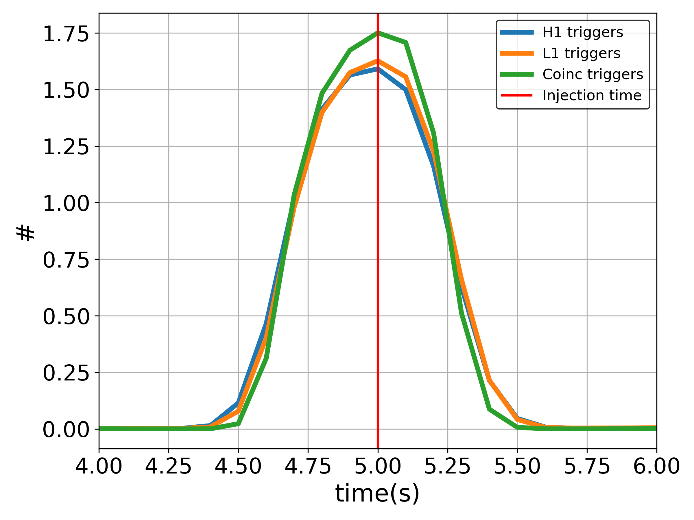
(a)	(b)

Figure 13: (a) This figure represents the cumulative histogram of L1 triggers, H1 triggers and the coincident triggers obtained for different detection probability thresholds($0.50$, $0.75$ and $0.90$). (b) This figure shows the density plots for the triggers obtained from two detectors (H1 and L1) noises and that of their coincidence outcome.

IV.3 Performance on O1, O2 and O3 data

Finally, we test the performance of our architecture against the real events obtained in O1, O2, and O3 data included in GWTC-1, GWTC-2, and GWTC-3 catalogs. To remind ourselves, we trained our architecture using the sensitivity curves of H1 and L1 based on the first three months of O3 data. Since our training is limited to the optimal SNR of range (10, 20), we only choose the events for which the network SNR lies in this specific range. Our architecture successfully detects all the chosen GW events in the first level of classification. Figures 14, 15 and 16 show the corresponding GW detection probability plots and their coincidence in H1 and L1 detectors. Most of the events are correctly classified during the second label of classification, based on their aligned and precession spins. The list of correctly classified aligned and precession events is listed in the tables 3, 5, 4. However, for the some of the events there is a disagreement between the two detectors in classifying them as aligned/precessing signals. In those cases, we would depend upon the result of the L1 detector as it is more sensitive compared to H1.

The parameter estimation studies on the catalog events does not say conclusively if the detected events are aligned or precessing, except for a few events. Below, we discuss our results vis-a-vis the predictions in the GW catalog papers.

Events from GWTC - 1: GW150914 is declared as precessing, while GW170104 and 170608 are declared to be aligned event. For GW170814, the two detectors show a disagreement in their results. However, none of the GW events in GWTC - 1 were reported to exhibit clear precession. The $\chi_{p}$ posteriors are broad, covering the entire domain from 0 to 1, and are overall similar to the conditioned priors (induced by the spin prior assumptions).

Events from GWTC-2: In our analysis of GWTC - 2 events, 5 have been declared as the precessing and 2 have as the aligned signals. While, for the other two events the two detectors show disagreement in their results. The events GW190412 and GW190521 were reported to indicate the precession with $\chi_{p}$ posterior distribution constrained away from zero. For these two events, our analysis is in agreement with this as well as with Fairhurst et al. Fairhurst et al. (2020).

Events from GWTC-3: All the four events have been declared to be precessing by both the detectors. GW200129_065458 has been reported to have an inferred $\chi_{p}$ of $0.54^{+0.39}_{-0.39}$. However, the inference has been shown to be sensitive to the waveform model used. For the other events the $\chi_{p}$ posteriors are broad and uninformative. However, the precession effects for those events can not be disregarded.

Figure 14: This figure shows the detection of GWTC1 catalogue BBH events in coincident with L1 and H1 detectors by using out coincident method. The events are chosen based on their network $\text{SNR}\geq 13.0$

Figure 15: This figure shows the detection of GWTC2 catalogue BBH events in coincident with L1 and H1 detectors by using out coincident method. The events are chosen based on their network $\text{SNR}\geq 13.0$

Figure 16: This figure shows the detection of GWTC3 catalogue BBH events in coincident with L1 and H1 detectors by using out coincident method. The events are chosen based on their network $\text{SNR}\geq 13.0$

V Conclusion

In this work we presented a machine learning-based detection scheme for the GW signals from BBH sources and identify them as aligned or precessing spin systems. We used synthetic as well as the real data for the training and testing of our machine learning based architecture. We first apply our method to the individual detectors and extend it to a multi-detector GW network. We developed an optimal configuration that provides binary classification between pure noise and noisy BBH signal from aligned or precessing spin systems with very high accuracy. Our architecture, at the first stage classified between the pure noise and noisy BBH signal. A signal obtained from the first level of classification is then used for further classification in terms of aligned or precessing signals at the second stage. We applied our scheme to the already detected events in gravitational wave transient catalogs (GWTC). The events were identified as both aligned as well as the precessing. The proposed scheme has an advantage: the prohibitive computational cost of performing a precession spin search can be reduced significantly compared to the classical matched-filter based approaches proposed in the literature Harry et al. (2016). Our approach can be used to develop a real-time search pipeline to detect the precession BBH systems. Further, our scheme is easily extendable to detect the precessing spin systems for the other binary systems (e.g., NSBH).