Guided Exploration in Reinforcement Learning
via Monte Carlo Critic Optimization

Abstract

The class of deep deterministic off-policy algorithms is effectively applied to solve challenging continuous control problems. However, current approaches use random noise as a common exploration method that has several weaknesses, such as a need for manual adjusting on a given task and the absence of exploratory calibration during the training process. We address these challenges by proposing a novel guided exploration method that uses a differential directional controller to incorporate scalable exploratory action correction. An ensemble of Monte Carlo Critics that provides exploratory direction is presented as a controller. The proposed method improves the traditional exploration scheme by changing exploration dynamically. We then present a novel algorithm exploiting the proposed directional controller for both policy and critic modification. The presented algorithm outperforms modern reinforcement learning algorithms across a variety of problems from DMControl suite.

1 Introduction

In reinforcement learning, exploration is a vital component of policy optimization. The method chosen to be an exploration strategy defines the interaction with the world, thus influences the final agent’s success being key in solving continuous (Zhang & Van Hoof, 2021), navigation (Mazoure et al., 2020) and hierarchical problems (Vigorito, 2016). On a high level, all exploration methods can be divided into undirected and directed ones (Thrun, 1992). The undirected methods provide random exploratory actions based on desired exploration-exploitation trade-off, while directed algorithms rely on information provided by a policy or a learned world model.

In real world, humans and animals seldom rely on random exploration of the environment, always pursuing some intrinsic motivation as safety (Tully et al., 2017), curiosity (Berlyne, 1966; Kidd & Hayden, 2015) or uncertainty minimization (Gershman, 2019). Equivalents of these psychological phenomena are successfully applied within corresponding research directions of reinforcement learning, forming the class of intrinsically-motivated algorithms (Garcıa & Fernández, 2015; Pathak et al., 2017). A scheme of such intrinsically motivating guided exploration is depicted in Figure 1, showing different directions of policy parameters change for the external- and intrinsic-reward objectives.

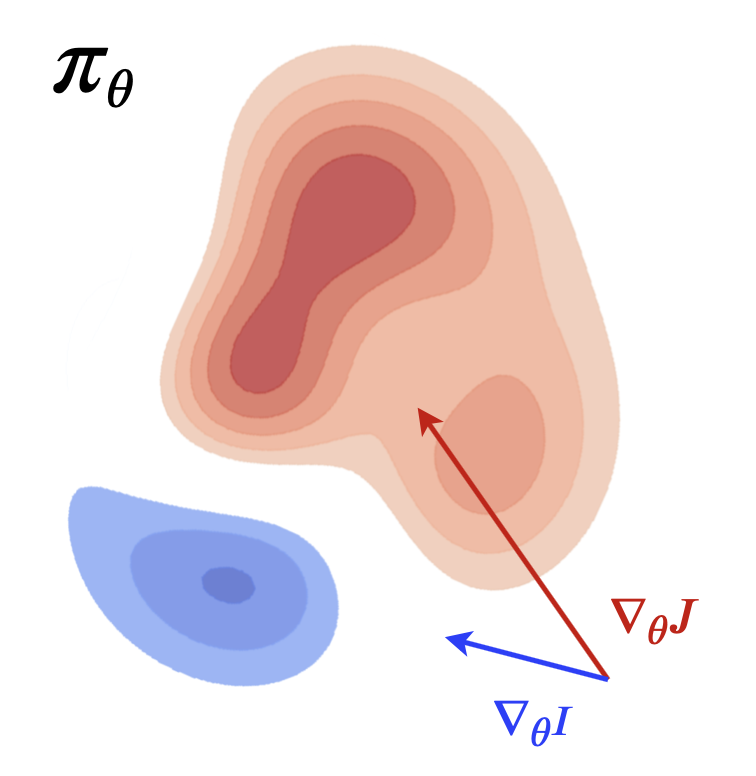
Figure 1: A scheme of a guided exploration model. Policy gradients $\nabla_{\theta}$ are directed by the final reward objective $J$ and corrected by an intrinsic objective $I$ facilitating directed exploration.

In the context of continuous control problems, the class of deep deterministic off-policy methods gains high popularity in the reinforcement learning community due to its implementation simplicity and state-of-the-art results. However, from an exploration perspective, such algorithms as DDPG (Lillicrap et al., 2015) and TD3 (Fujimoto et al., 2018) use Gaussian or time-dependent Ornstein-Uhlenbeck noise that is applied to deterministic action. While being a simple and rather effective exploration tool, the methods based on random noise suffer from three limitations. Firstly, in high dimensional environments random exploration is an inefficient strategy to achieve certain regions of interest in the state-space that can lead to success (Burda et al., 2018). Secondly, the algorithms discussed apply noise with the same mean and deviation during the whole period of policy optimization. Being a crucial instrument in the beginning of parameter search, excessive exploration may hurt the policy performance to reach its optimal condition. Finally, the aforementioned methods apply noise of the same magnitude for all actions, whereas actions in continuous control often relate to the entities of different scales.

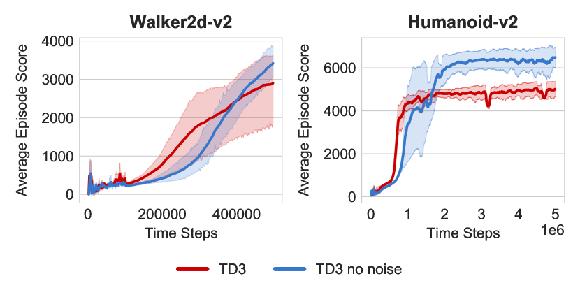
Figure 2: Preliminary motivation experiment. The performance of the original version of TD3 algorithm compared with a variant without exploration noise.

To illustrate the sub-optimality of conventional random exploration and justify our motivation we consider the TD3 algorithm performance on two continuous control domains, Walker2d-v2 and Humanoid-v2 (Brockman et al., 2016). We compare the original version of TD3 and a variant without any noise applied during action selection and calculation of a critic value. Original TD3 provides poor performance compared with the version without any exploration noise (Figure 2). This simple experiment demonstrates that current Gaussian-based exploration can hurt the agent’s performance. Nevertheless, the total absence of exploration may also lead to lower episodic reward, as our later experiments show. We aim to develop an effective method of directed exploration that enhances the results of deterministic off-policy algorithms.

We address the mentioned weaknesses of random exploration by introducing a directional controller that is able to guide a policy in a meaningful exploratory direction. Specifically, we propose to use an ensemble of Q-function approximations trained to predict Monte Carlo Q-values as such a controller. By optimizing multiple independent predictions and using the action gradient from calculated variance we are able to obtain an uncertainty estimate for a given state. Based on this gradient we provide an exploratory action correction towards the most unexplored environment regions.

The contribution of this paper is twofold. First, we present a method for a guided exploration that can substitute Gaussian noise and be incorporated into any off-policy deterministic algorithm. We show that the proposed exploration improves over other exploration methods on a set of continuous control tasks. Second, we present a novel algorithm that exploits the proposed uncertainty-based directional controller for both actor and critic parts of model architecture. The proposed method demonstrates superior results compared with modern reinforcement learning algorithms on a set of tasks from DMControl suite.

Following the guidelines of reproducibility of reinforcement learning algorithms (Henderson et al., 2018) we report the results on a large number of seeds and release the source code alongside raw data of learning curves .

2 Preliminaries

We consider a standard reinforcement learning (RL) setup, in which an agent interacts with an environment $\mathcal{E}$ at discrete time steps aiming to maximize the reward signal. The environment is a Markov Decision Process (MDP) that can be defined as $\langle\mathcal{S},\mathcal{A},\mathcal{R},\rho,\mathcal{\gamma}\rangle$, where $\mathcal{S}$ is a state space, $\mathcal{A}$ is an action space, $\mathcal{R}$ is a reward function, $\rho$ is a transition dynamics and $\gamma\in[0,1]$ is a discount factor. At time step $t$ the agent receives state $s_{t}\in\mathcal{S}$ and performs action $a_{t}\in\mathcal{A}$ according to policy $\pi$, a distribution of $a$ given $s$ that leads the agent to the next state $s_{t+1}$ according to the transition probability $\rho(s_{t+1}|s_{t},a_{t})$. After providing the action to $\mathcal{E}$, the agent receives a reward $r_{t}\sim\mathcal{R}(s_{t},a_{t})$. The discounted sum of rewards during the episode is defined as a return $R_{t}=\sum_{i=t}^{T}\gamma^{i-t}r(s_{i},a_{i})$.

The RL agent aims to find the optimal policy $\pi_{\theta}$, with parameters $\theta$, which maximizes the expected return from the initial distribution $J(\theta)=\operatorname{\mathbb{E}}_{s_{i}\sim\rho_{\pi},a_{i}\sim\pi_{\theta}}[R_{0}]$. The action-value function $Q$ is at core of many RL algorithms and denotes the expected return when performing action $a$ from the state $s$ following the current policy $\pi$:

$$Q^{\pi}(s,a)=\operatorname{\mathbb{E}}_{s_{i}\sim\rho_{\pi},a_{i}\sim\pi}\left[R_{t}|s,a\right].$$ (1)

In continuous control problems the actions are real-valued and the policy $\pi_{\theta}$ can be updated taking the gradient of the expected return $\nabla_{\theta}J(\theta)$ with deterministic policy gradient algorithm  (Silver et al., 2014):

$$\nabla_{\theta}J(\theta)=\operatorname{\mathbb{E}}_{s\sim\rho_{\pi}}\left[\nabla_{a}Q^{\pi}(s,a)|_{a=\pi(s)}\nabla_{\theta}\pi_{\theta}(s)\right].$$ (2)

The class of actor-critic methods operates with two parameterized functions. An actor represents policy $\pi$ and the critic is the Q-function. The critic is updated with temporal difference learning by iteratively minimizing the Bellman error  (Watkins & Dayan, 1992):

$$J_{Q}=\operatorname{\mathbb{E}}\left[(Q(s_{t},a_{t})-(r+\gamma Q(s_{t+1},a_{t+1})))^{2}\right].$$ (3)

In deep reinforcement learning, the parameters of Q-function are modified with additional frozen target network $Q_{\theta^{\prime}}$ which is updated by $\tau$ proportion to match the current Q-function $\theta^{{}^{\prime}}\leftarrow\tau\theta+(1-\tau)\theta^{{}^{\prime}}$

$$J_{Q}=\operatorname{\mathbb{E}}\left[(Q(s_{t},a_{t})-Q^{\prime})^{2}\right],$$ (4)

where

$$Q^{\prime}=r(s_{t},a_{t})+\gamma Q_{\theta^{\prime}}(s_{t+1},a^{\prime}),a^{\prime}\sim\pi_{\theta^{{}^{\prime}}}(s_{t+1}).$$ (5)

The actor is learned to maximize the current $Q$ function:

$$J_{\pi}=\operatorname{\mathbb{E}}\left[Q(s,\pi(s))\right].$$ (6)

In this work, we focus on an off-policy version of actor-critic algorithms, proven to have better sample complexity (Lillicrap et al., 2015). Within this approach, the actor and the critic are updated with samples from a different policy, allowing to re-use the samples collected from the environment. The mini-batches are sampled from the experience replay buffer (Lin, 1992).

In off-policy Q-learning, actions are selected greedily w.r.t. maximum Q-value thus producing overestimated predictions. An effective way to alleviate this issue is keeping two separate Q-function approximators and taking a minimal one during the optimization (Van Hasselt et al., 2016). Modern actor-critic methods (Fujimoto et al., 2018; Haarnoja et al., 2018b) independently optimize two critics $Q^{1},Q^{2}$ with identical structure and use the lower estimate during the calculation of the target $Q^{\prime}$:

$$Q^{\prime}=r(s_{t},a_{t})+\gamma\min{[Q^{1}_{\theta^{\prime}}(s_{t+1},a^{\prime}),Q^{2}_{\theta^{\prime}}(s_{t+1},a^{\prime})]}.$$ (7)

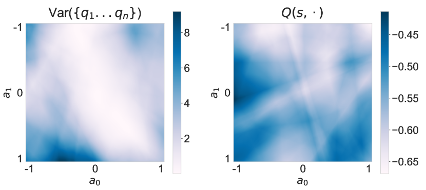
Figure 3: Visualization of uncertainty estimation (left) and critic prediction (right) at the same state on 2D action plane. Environment: point-mass-easy.

3 Method of Guided Exploration

On a high level, our agent consists of two components: an actor-critic part to provide a deterministic policy and a directional controller that modifies policy output action to facilitate directed exploration. The deterministic policy $\pi_{\theta}(s)$ is parameterized by $\theta$ and optimizes reward maximization to produce a base action $a^{\mathrm{b}}$. The directional controller $\psi$ optimizes auxiliary intrinsic objective to produce an exploratory action correction $a^{\mathrm{e}}$. The policy and the directional controller are jointly optimized to produce an additive action to collect transitions for off-policy updates:

$$a\coloneqq a^{\mathrm{b}}+a^{\mathrm{e}},a^{\mathrm{b}}\sim\pi_{\theta}(s)$$ (8)

For the actor-critic part, we use the TD3 algorithm (Fujimoto et al., 2018) as a backbone.

3.1 Directional Controller

The directional controller $\mathrm{DC}_{\omega}(s|\theta)$ is parameterized by $\omega$ and conditioned on policy parameters $\theta$. The proposed controller features an ensemble of Q-function approximators $\{q_{1}(s,a),...,q_{n}(s,a)\}$ that predicts the collected Monte Carlo Q-values. The values for the update are sampled from a small experience replay buffer $\mathcal{D}_{MC}$ with recent trajectories collected by the policy. Given $n$ ensemble predictions, the controller $\mathrm{DC}$ estimates prediction uncertainty as the ensemble disagreement:

$$\psi_{\omega}(s|\theta)\coloneqq{\textrm{Var}}\,(\{q_{1}(s,a),...,q_{n}(s,a))\}),$$ (9)

where $q_{i}(s,a)=\operatorname{\mathbb{E}}_{s\sim\mathcal{D}_{MC},a\sim\pi_{\theta}}[R],i\in[1..n]$. This disagreement reflects both epistemic uncertainty of controller parameters and aleatory uncertainty of the collected Monte Carlo Q-values. During optimization, controller’s objective is to reduce uncertainty in a supervised fashion by minimizing square distance between the predicted and collected returns:

$$J_{\phi}=\sum^{n}_{i=1}(Q^{MC}(s,a)-q_{i}(s,a))^{2},$$ (10)

where $(s,a)$ is a state-action pair sampled from $\mathcal{D}_{MC}$ with the corresponding Monte Carlo Q-value $Q^{MC}(s,a)$. Taking the gradient of the controller w.r.t. action, we obtain the direction towards maximizing the uncertainty under current controller parameters $\omega$:

$$\nabla_{a}\psi_{\omega}=\nabla_{a}{\textrm{Var}}\,(\{q_{1}(s,a),...,q_{n}(s,a))\})\lvert_{a\sim\pi_{\theta}(s).}$$ (11)

This gradient value is at the core of exploratory action $a^{\mathrm{e}}$, as it identifies the direction towards the most unexplored environment regions. Figure 3 depicts the surface of the uncertainty estimation value returned by $\psi(s)$ and the critic prediction $Q(s,\cdot)$ for the point_mass-easy task, where $|\mathcal{A}|=2$. The visualization is performed after 1e5 time steps with fixed state $s$ and a set of actions $a\in[a_{MIN},a_{MAX}]$. The surfaces show different highest points, making $a^{\mathrm{b}}$ and $a^{\mathrm{e}}$ have different directions.

We use Monte Carlo Q-value approximation as a directional controller for two reasons. First, it is differentiable w.r.t action, allowing to obtain action gradient. Second, in contrast with model-based dynamics (Janner et al., 2019) and curiosity (Pathak et al., 2017) approaches, which require either the next state or the next action to compute the intrinsic signal, we need only the current state-action pair to obtain a plausible action direction. Since the directional controller to modify the exploratory action is applied, we do not have an access to the next transition as in approaches that incorporate intrinsic signal during the off-policy update step.

3.2 Calculating action correction

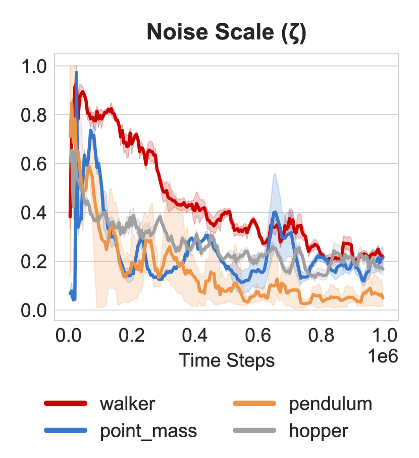
(a) Dynamics of scaling coefficient $\zeta$. Values are averages across action dimensions.

(b) Dynamically calibrated exploratory action correction $a^{\mathrm{e}}$ during policy optimization.

During policy optimization the agent sequentially performs a base action $a^{\mathrm{b}}\sim\pi_{\theta}(s)$. Given the state $s$ and policy parameters $\theta$, the directional controller provides the base action gradient towards exploration objective $\nabla_{a^{\mathrm{b}}}\psi_{\omega}(s|\theta)$. Here we describe the procedure of obtaining action correction $a^{\mathrm{e}}$ based on this gradient. To connect gradient value $\nabla a^{\mathrm{b}}$ with action scales we perform the following scaling procedure:

$$a^{\mathrm{e}}=\frac{\nabla a^{\mathrm{b}}}{\lVert\nabla a^{\mathrm{b}}\lVert_{2}}\cdot\epsilon\cdot\zeta,$$ (12)

where $\epsilon$ is denormalization constant and $\zeta$ is a scaling factor. The denormalization constant $\epsilon$ is to scale normalized gradient values to the practical magnitude of actions for a given task. It is possible to set this constant to the value that corresponds to exploration magnitude used in (Lillicrap et al., 2015; Fujimoto et al., 2018), obtaining a directional vector of a scale required. However, with this only modification action correction vector would be fixed in its magnitude during the learning process. As a solution, we set $\epsilon$ to the magnitude of fully exploratory vector of random actions sampled uniformly:

$$\epsilon\coloneqq\mathbb{E}[\lVert a\lVert_{2}],a\sim\mathcal{U}(a_{MIN},a_{MAX})$$ (13)

with the following multiplying by the dynamic scaling factor $\zeta$. We pose two requirements on the scaling factor:

• It should be bounded with $\zeta_{i}\in[0..1],i\in[1..|\mathcal{A}|]$, with $0$ corresponding to the absence of exploration and $1$ corresponding to the random action selection.

• It should change dynamically within the policy optimization.

To satisfy both requirements we support two statistical quantities during the learning process: the running deviation of $\nabla a^{\mathrm{b}}$ for the last $N$ time steps $\sigma_{N}(\nabla a^{\mathrm{b}})$ and its maximum value ${\textrm{max}}\,[\sigma(\nabla a^{\mathrm{b}})]$ for all seen deviation gradient values during the learning, resulting in:

$$\zeta_{i}=\frac{\sigma_{N}(\nabla a_{i}^{\mathrm{b}})}{{\textrm{max}}\,[\sigma(\nabla a_{i}^{\mathrm{b}})]},i\in[1..|\mathcal{A}|].$$ (14)

Large values of gradient deviation between adjacent actions from a small running window of size $N$ show uncertainty of the ensemble thus reflecting the need for more intensified exploration. The scaling factor is of dimension $|\mathcal{A}|$, facilitating keeping the individual scale for each element of a continuous action vector.

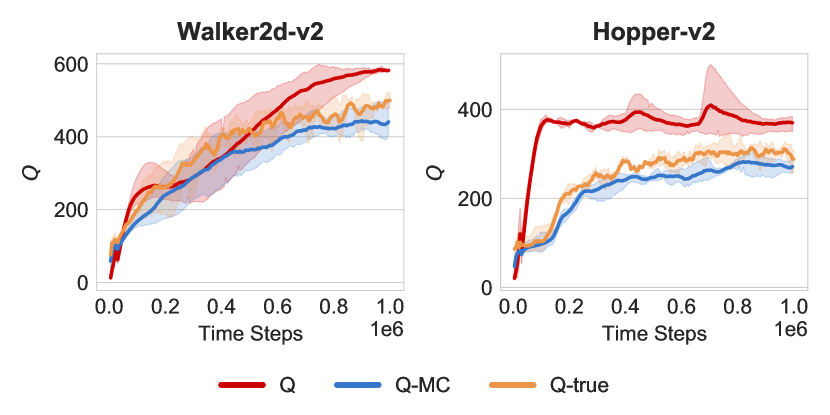
Figure 5: An illustration of Q-value overestimation. The true value of $Q$-function (Q-true) lies between overestimated critic prediction (Q) and underestimated Monte Carlo prediction (Q-MC).

The dynamics of exploratory action $a^{\mathrm{e}}$ during the learning process on different tasks is depicted in Figure 4(a). In the beginning of the training, the scaling factor is close to maximum action bound enhancing aggressive exploration. During the policy and the directional controller optimization $\zeta$ decreases leading the policy to more exploitation-inclined behavior. Notably, the dynamics of the scaling factor are not identical between environments. An example of action correction values $a^{\mathrm{e}}$ for the walker-run task are depicted in Figure 4(b).

4 MOCCO Algorithm

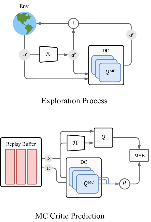
Figure 6: MOCCO: A role of the directional controller (DC) during exploration (top) and critic optimization (bottom).

Based on the presented technique of guided exploration, we propose a novel deep reinforcement learning algorithm Monte Carlo Critic Optimization (MOCCO) that incorporates an ensemble of Monte Carlo critics not only for the actor, as an exploratory module, but also for the critic to alleviate Q-value overestimation. Several works have studied Q-value overestimation in continuous control setting and have presented techniques to alleviate the issue (Ciosek et al., 2019; Kuznetsov et al., 2020; Kuznetsov & Filchenkov, 2021). Here, we propose to use a mean from the ensemble of Monte Carlo values as a second pessimistic Q-value estimate during critic optimization, resulting in the following critic’s objective:

$$J_{Q}=(Q-Q^{\prime})^{2}+(Q-\beta\cdot Q^{MC})^{2},$$ (15)

where $Q^{MC}=\mu(\{q_{1},...,q_{n}\})$, and $\beta$ is a coefficient controlling an impact of the pessimistic estimate. For the given state-action pair $(s,a)$ the critic estimate $Q(s,a)$ is generally greater than the corresponding Monte Carlo estimate $Q^{MC}$, as the latter predicts estimates of the past sub-optimal policies. To illustrate this, we measure the following quantities during the learning process on tasks Walker2d-v2 and Hopper-v2:

• TD-based bootstrapped Q-value approximation as averaged critic $Q$ prediction. Only a single critic is optimized during the TD optimization.

• True Q-value estimate as a discounted return of the current policy starting from given state-action pair.

• Monte Carlo Critic Q-value estimate as an averaged prediction of $Q^{MC}$.

All three quantities are averages across the batch size of 256 that are collected each 5e3 time steps and reported from multiple seeds. Figure 5 shows the dynamics of predictions on 1M time steps. Monte Carlo prediction (Q-MC) has lower value than both TD-based (Q) and true Q-estimate (Q-true) values, while TD-based prediction is generally higher than the true estimate.

Algorithm 1 MOCCO

1:  Initialize actor $\pi_{\theta^{\pi}}$, critic $Q_{\theta^{Q}}$, target critic $Q^{{}^{\prime}}_{\theta^{Q^{{}^{\prime}}}}$

2:  Initialize directional controller $\mathrm{DC}_{\omega}=\{q_{1},...,q_{k}\}$

3:  Initialize replay buffer $\mathcal{B}$, episodic buffer $\mathcal{B}_{E}$

4:  Initialize smaller buffer $\mathcal{B}^{MC}$ for the most recent steps

5:  for t=1 to T do

6:     Select action with guided noise $a=a^{\mathrm{b}}+a^{\mathrm{e}}$,

7:     $a^{\mathrm{b}}\sim\pi_{\theta^{\pi}}(s),a^{\mathrm{e}}\sim\mathrm{DC}_{\omega}$

8:     Receive next state $s^{{}^{\prime}}$, reward $r$, terminal signal $d$

9:     if $d$ then

10:        for i=1 to $|\mathcal{B}_{E}|$ do

11:           Calculate discounted episodic return $R_{i}$

12:           Store $(s_{i},a_{i},r_{i},s^{{}^{\prime}}_{i},d_{i})$ in $\mathcal{B}$

13:           Store $(s_{i},a_{i},R_{i})$ in $\mathcal{B}^{MC}$

14:        end for

15:        Free $\mathcal{B}_{E}$

16:     end if

17:     Sample mini-batch from $\mathcal{B}$: $[s_{b},a_{b},r_{b},s_{b}]$ and

18:     update critic $Q$: $J_{Q}=(Q-Q^{\prime})^{2}+\beta(Q-Q^{MC})^{2}$

19:     Sample mini-batch from $\mathcal{B}^{MC}$: $[s_{b},a_{b},R_{b}]$ and

20:     update $\mathrm{DC}_{\omega}$: $J_{\mathrm{DC}}=\sum_{i}^{k}(q_{i}-R_{b})^{2}$

21:     if t mod 2 then

22:        Update policy $\pi_{\theta}^{\pi}$

23:        Update target critic $\theta^{Q}{{}^{{}^{\prime}}}\leftarrow\tau\theta^{Q}+(1-\tau)\theta^{Q^{{}^{\prime}}}$

24:     end if

25:  end for

26:  return $\theta^{\pi}$

In reinforcement learning, Monte Carlo estimates have high variance and low bias, whereas one-step TD methods have less variance but can be biased. Here, we combine both methods during Q-function optimization. Empirically we show that the true Q-value estimate lies between $Q$ and $Q^{MC}$, therefore it is beneficial to use both estimates to balance between over- and underestimation.

The role of the directional controller (DC) during the exploration and critic optimization is schematically depicted in Figure 6. During action selection, DC provides directed exploration i.e. it is applied on-policy. During off-policy update steps, DC is used to provide a second estimate for current Q-function optimization.

Practically, the MOCCO algorithm is based on TD3 with the following differences: (1) it uses guided exploration during action selection; (2) it does not use second TD critic; (3) the mean of MC-critics ensemble is used during the critic optimization. Full pseudo-code is presented in Algorithm 1.

5 Experiments

First, we demonstrate that the proposed method improves conventional random noise-based exploration using TD3 algorithm. Next, we show experimental results for MOCCO. We perform an ablation study to identify the impact of each proposed algorithmic component on final success and demonstrate the comparative evaluation results.

Table 1: A comparison of exploration approaches. Average episodic score from 10 trials. Each trial is a mean of the last 10 episodes.

Task	no expl	normal	OU	GE
point_mass	661.79	737.72	600.20	814.22
walker-walk	940.49	947.18	936.67	962.56
walker-run	535.56	586.53	603.93	621.07
hopper-stand	46.05	6.13	21.55	54.66
hopper-hop	29.20	48.95	28.48	45.57

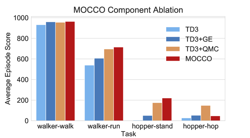
Figure 7: Contribution of different components of MOCCO algorithm.

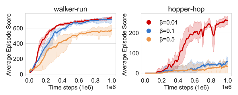
(a) $\beta$ hyperparameter.

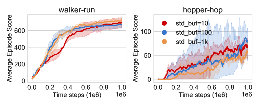
(b) The size $N$ of the running window for calculating $\sigma_{N}(\nabla a)$.

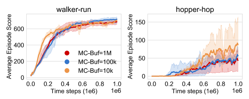
(c) The size of $\mathcal{D}_{MC}$.

Figure 8: The impact of different hyperparameter values.

5.1 Guided Exploration for Off-Policy Deterministic Algorithms

In this experiment, we show that guided exploration improves over the traditional Gaussian-based exploration method. To do so, we use TD3 as a baseline algorithm and vary the type of applied exploratory noise during the action selection process. Table 1 shows the results of the following scenarios: actions are sampled without noise (no expl), with Normal Gaussian noise (normal), temporally correlated noise drawn from an Ornstein-Uhlenbeck process (OU), and with proposed guided exploration method (GE). For normal Gaussian and Ornstein-Uhlenbeck noise, we use parameters reported in (Haarnoja et al., 2018b; Lillicrap et al., 2015) correspondingly. We run each algorithm 10 times with different random seeds. Within each run, the reported value is the mean of 10 evaluations of the same policy from different environment initialization. Results demonstrate higher rewards of guided exploration over the conventional approaches for all environments except hopper-hop.

5.2 MOCCO: Ablation Study

The aim of this experiment is to identify the impact of each component on the overall success of the presented algorithm. We study the contribution of guided exploration as a substitution of the Gaussian noise (TD3 + GE), the contribution of the proposed critic objective featuring Monte Carlo critic estimate (TD3 + QMC), and of both features combined (MOCCO).

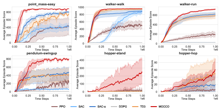
Figure 9: Learning curves of evaluation algorithms. The shading region shows standard deviation across seeds. Curves are smoothed with a 10-point moving average for clarity.

Table 2: Evaluation results as the average of the last 10 episodes. $\pm$ denotes standard deviation across seeds.

Env	PPO	SAC	SAC-$\alpha$	DDPG	TD3	MOCCO
point_mass	431.71	437.77	795.59	0.81	737.72	882.84 $\pm$ 9.17
walker-walk	505.54	884.88	892.76	26.13	947.18	959.12 $\pm$ 12.07
walker-run	187.13	26.27	618.34	26.68	586.53	722.10$\pm$ 23.78
pendulum-swingup	261.970	70.61	473.64	11.96	424.22	795.73 $\pm$ 41.84
hopper-stand	17.84	5.94	5.94	11.02	6.13	249.53 $\pm$ 263.34
hopper-hop	5.12	0.06	19.43	0.17	48.95	60.98 $\pm$ 42.22

Figure 7 shows results for walker-walk, walker-run, hopper-stand, hopper-hop on 5 random seeds. Results show that each component improves the results of TD3 algorithm on all tasks and a combination of features provides better performance than their sole contributions on 3 out of 4 tasks.

Next, we vary hyperparameters introduced by MOCCO to identify algorithm robustness on two tasks: walker-walk and hopper-hop. We study different values of the coefficient controlling MC critic impact ($\beta$), the size $N$ of the buffer used for calculating the running deviation of action gradient $\sigma_{N}(\nabla a)$, and the size of reduced replay buffer $\mathcal{B}^{MC}$ on which the ensemble of MC critics is trained. Figure 8 shows that MOCCO is robust to the hyperparameter change, except the case of varying $\beta$ for hopper-hop.

We demonstrate comparative results of MOCCO algorithm on 6 control problems from DMControl (Tassa et al., 2018) benchmark: point_mass-easy, walker-walk, walker-run, pendulum-swingup, hopper-stand, hopper-hop. We compare the proposed approach with off-policy algorithms DDPG, TD3, SAC (Haarnoja et al., 2018a) and on-policy PPO (Schulman et al., 2017) algorithm. For off-policy algorithms, we run 1M environment time steps on each environment, collecting episode scores for every 2e3 steps. Each episode score is an average of 10 runs of a policy without exploration from different environment seeds. Each algorithm is run 10 times with different seeds with reported standard deviation. For PPO, we run the training process 10 times with different environmental and algorithmic seeds with the following averaging.

We use the official implementation of TD3 as a baseline. For DDPG, we use the implementation from TD3, denoted as ”DDPG”. We extend the TD3 code to entropy optimization for SAC deriving. For PPO results we use the implementation from (Kostrikov, 2018).

We use Adam optimizer (Kingma & Ba, 2014) with the learning rate 3e-4 for all algorithms. For a fair comparison, we use the same network parameters from the (Fujimoto et al., 2018). All networks have 2 hidden layers of size 256 and ReLU non-linearity (Glorot et al., 2011). For SAC we run two versions, first with fixed entropy coefficient equal to 0.2 (proposed in (Achiam, 2018)) and auto tunable entropy (SAC-$\alpha$) from (Haarnoja et al., 2018b). We use mini-batch size 256 for all algorithms.

For MOCCO, we set the size of $\mathcal{D}_{MC}$ to 1e5 transitions, and the size of buffer $N$ for calculating deviations used in the scaling factor $\zeta$ to 1000. We use 3 critics in the ensemble as our experiments have not provided benefits from an increased number of critics. The $\beta$ coefficient controlling an impact of MC-critic is set to 0.1.

Table 2 reports the average of episodic scores for the last 10 episodes. The corresponding learning curves are presented in Figure 9. MOCCO outperforms other approaches, sometimes with significant margins, e.g. for pendulum and hopper-stand.

6 Related Work

The problem of efficient exploration has a long-standing history in reinforcement learning. Early approaches suggest incorporating random exploratory strategies (Moore, 1990; Sutton, 1990; Barto et al., 1991; Williams, 1992) which have theoretical grounds but are not always scalable to complex environments with high-dimensional inputs. The broad class of directed exploration algorithms, first proposed in (Thrun, 1992), studies an approach of guiding a policy towards certain regions with specific knowledge of the learning process.

Numerous works on directed exploration study intrinsic reward, where the learning process relies on some intrinsic signal. Examples of exploration based on intrinsic reward include algorithms based on information gain (Little & Sommer, 2013; Mobin et al., 2014), curiosity (Deci et al., 1981; Pathak et al., 2017), and uncertainty-minimization (Schmidhuber, 1991; Houthooft et al., 2016). (Badia et al., 2019) propose to use episodic memory as a source of the intrinsic signal and optimize multiple policies, some of which are guided by exploratory goals and others are fully exploitative. In contrast with many intrinsic-reward approaches, our method does not modify the reward with additional dense signal nor modifies the policy, but rather optimizes the intrinsic objective independently only to correct exploratory action.

The work of (Pathak et al., 2019) shows that exploration can be key in achieving high sample efficiency required for real-world setup. The authors use an ensemble of forward dynamics models that produces disagreement as an intrinsic reward. Incorporation of such a disagreement signal results in an effective exploration, allowing robots to solve object interaction tasks from scratch in real-time.

Apart from the directed exploration based on intrinsic objective, several works have proposed methods with a different perspective. (Ciosek et al., 2019) addresses the notion of pessimistic underexploration that comes from optimizing a lower bound in critic update. By approximating the upper bound of state-action function and using it during exploration the proposed method avoids underexploration and achieves higher sample efficiency. Some works study the approach of exploration in policy parameter space rather than in action space (van Hoof et al., 2017; Fortunato et al., 2018; Zhang & Van Hoof, 2021). Finally, a number of works study exploration under goal-reaching angle, where the agent explores environment by learning to achieve seen (Florensa et al., 2018), generated (Nair et al., 2018; Sukhbaatar et al., 2018), or specifically unseen (Mendonca et al., 2021) state regions.

A comprehensive review of exploration in reinforcement learning can be found in (Amin et al., 2021). Following the suggested taxonomy, the method presented in this paper falls into the category of ”reward-free intrinsically-motivated” exploration i.e. not using an extrinsic reward for exploratory purpose, but relying on intrinsic signal to explore novel world regions.

7 Discussion

We presented a method for directed exploration that improves off-policy deterministic algorithms by adding exploratory action correction to the base policy action. By using a differential controller conditioned on policy parameters we direct exploration towards the regions of interest and dynamically calibrate the magnitude of exploratory correction during the learning process. The proposed exploration method does not require rigorous hyperparameter turning due to the dependence on a learnable intrinsic signal that reflects given environmental uncertainty. We provide empirical results that validate the efficacy of the proposed method on a range of continuous control tasks. Our approach achieves a higher reward than methods dependent on a random noise. We further presented MOCCO, a novel deep reinforcement learning algorithm based on the proposed exploration method. Experiments showed that MOCCO outperforms modern off-policy actor-critic methods on a set of DMControl suite tasks.

We note that the proposed directional controller based on optimizing Monte Carlo Q-values can be substituted by a different differential model. For example, such a controller can be presented as a form of forward or inverse model dynamics, shifting the focus to model-based reinforcement learning. Another promising direction is to present the directional controller as a differential memory module, connecting the direction of the external agent’s memory with efficient exploration. We believe that the proposed exploration technique will help to tackle problems that require careful dynamic exploration.

References

- Achiam (2018) Achiam, J. Spinning Up in Deep Reinforcement Learning. 2018.
- Amin et al. (2021) Amin, S., Gomrokchi, M., Satija, H., van Hoof, H., and Precup, D. A survey of exploration methods in reinforcement learning. arXiv preprint arXiv:2109.00157, 2021.
- Badia et al. (2019) Badia, A. P., Sprechmann, P., Vitvitskyi, A., Guo, D., Piot, B., Kapturowski, S., Tieleman, O., Arjovsky, M., Pritzel, A., Bolt, A., et al. Never give up: Learning directed exploration strategies. In International Conference on Learning Representations, 2019.
- Barto et al. (1991) Barto, A. G., Bradtke, S. J., and Singh, S. P. Real-time learning and control using asynchronous dynamic programming. University of Massachusetts at Amherst, Department of Computer and …, 1991.
- Berlyne (1966) Berlyne, D. E. Curiosity and exploration. Science, 153(3731):25–33, 1966.
- Brockman et al. (2016) Brockman, G., Cheung, V., Pettersson, L., Schneider, J., Schulman, J., Tang, J., and Zaremba, W. Openai gym. arXiv preprint arXiv:1606.01540, 2016.
- Burda et al. (2018) Burda, Y., Edwards, H., Storkey, A., and Klimov, O. Exploration by random network distillation. arXiv preprint arXiv:1810.12894, 2018.
- Ciosek et al. (2019) Ciosek, K., Vuong, Q., Loftin, R., and Hofmann, K. Better exploration with optimistic actor-critic. In Proceedings of the 33rd International Conference on Neural Information Processing Systems, pp. 1787–1798, 2019.
- Deci et al. (1981) Deci, E. L., Nezlek, J., and Sheinman, L. Characteristics of the rewarder and intrinsic motivation of the rewardee. Journal of personality and social psychology, 40(1):1, 1981.
- Florensa et al. (2018) Florensa, C., Held, D., Geng, X., and Abbeel, P. Automatic goal generation for reinforcement learning agents. In International conference on machine learning, pp. 1515–1528. PMLR, 2018.
- Fortunato et al. (2018) Fortunato, M., Azar, M. G., Piot, B., Menick, J., Hessel, M., Osband, I., Graves, A., Mnih, V., Munos, R., Hassabis, D., et al. Noisy networks for exploration. In International Conference on Learning Representations, 2018.
- Fujimoto et al. (2018) Fujimoto, S., Hoof, H., and Meger, D. Addressing function approximation error in actor-critic methods. In International Conference on Machine Learning, pp. 1587–1596. PMLR, 2018.
- Garcıa & Fernández (2015) Garcıa, J. and Fernández, F. A comprehensive survey on safe reinforcement learning. Journal of Machine Learning Research, 16(1):1437–1480, 2015.
- Gershman (2019) Gershman, S. J. Uncertainty and exploration. Decision, 6(3):277, 2019.
- Glorot et al. (2011) Glorot, X., Bordes, A., and Bengio, Y. Deep sparse rectifier neural networks. In Proceedings of the fourteenth international conference on artificial intelligence and statistics, pp. 315–323. JMLR Workshop and Conference Proceedings, 2011.
- Haarnoja et al. (2018a) Haarnoja, T., Zhou, A., Abbeel, P., and Levine, S. Soft actor-critic: Off-policy maximum entropy deep reinforcement learning with a stochastic actor. In Dy, J. and Krause, A. (eds.), Proceedings of the 35th International Conference on Machine Learning, volume 80 of Proceedings of Machine Learning Research, pp. 1861–1870. PMLR, 10–15 Jul 2018a.
- Haarnoja et al. (2018b) Haarnoja, T., Zhou, A., Hartikainen, K., Tucker, G., Ha, S., Tan, J., Kumar, V., Zhu, H., Gupta, A., Abbeel, P., et al. Soft actor-critic algorithms and applications. arXiv preprint arXiv:1812.05905, 2018b.
- Henderson et al. (2018) Henderson, P., Islam, R., Bachman, P., Pineau, J., Precup, D., and Meger, D. Deep reinforcement learning that matters. In Proceedings of the AAAI conference on artificial intelligence, volume 32, 2018.
- Houthooft et al. (2016) Houthooft, R., Chen, X., Duan, Y., Schulman, J., De Turck, F., and Abbeel, P. Vime: Variational information maximizing exploration. Advances in Neural Information Processing Systems, 29:1109–1117, 2016.
- Janner et al. (2019) Janner, M., Fu, J., Zhang, M., and Levine, S. When to trust your model: Model-based policy optimization. Advances in Neural Information Processing Systems, 32, 2019.
- Kidd & Hayden (2015) Kidd, C. and Hayden, B. Y. The psychology and neuroscience of curiosity. Neuron, 88(3):449–460, 2015.
- Kingma & Ba (2014) Kingma, D. P. and Ba, J. Adam: A method for stochastic optimization. arXiv preprint arXiv:1412.6980, 2014.
- Kostrikov (2018) Kostrikov, I. Pytorch implementations of reinforcement learning algorithms. https://github.com/ikostrikov/pytorch-a2c-ppo-acktr-gail, 2018.
- Kuznetsov et al. (2020) Kuznetsov, A., Shvechikov, P., Grishin, A., and Vetrov, D. Controlling overestimation bias with truncated mixture of continuous distributional quantile critics. In International Conference on Machine Learning, pp. 5556–5566. PMLR, 2020.
- Kuznetsov & Filchenkov (2021) Kuznetsov, I. and Filchenkov, A. Solving continuous control with episodic memory. In Proceedings of the Thirtieth International Joint Conference on Artificial Intelligence, IJCAI-21, pp. 2651–2657, 8 2021. Main Track.
- Lillicrap et al. (2015) Lillicrap, T. P., Hunt, J. J., Pritzel, A., Heess, N., Erez, T., Tassa, Y., Silver, D., and Wierstra, D. Continuous control with deep reinforcement learning. arXiv preprint arXiv:1509.02971, 2015.
- Lin (1992) Lin, L.-J. Self-improving reactive agents based on reinforcement learning, planning and teaching. Machine learning, 8(3-4):293–321, 1992.
- Little & Sommer (2013) Little, D. Y.-J. and Sommer, F. T. Learning and exploration in action-perception loops. Frontiers in neural circuits, 7:37, 2013.
- Mazoure et al. (2020) Mazoure, B., Doan, T., Durand, A., Pineau, J., and Hjelm, R. D. Leveraging exploration in off-policy algorithms via normalizing flows. In Conference on Robot Learning, pp. 430–444. PMLR, 2020.
- Mendonca et al. (2021) Mendonca, R., Rybkin, O., Daniilidis, K., Hafner, D., and Pathak, D. Discovering and achieving goals via world models. Advances in Neural Information Processing Systems, 34, 2021.
- Mobin et al. (2014) Mobin, S. A., Arnemann, J. A., and Sommer, F. Information-based learning by agents in unbounded state spaces. Advances in Neural Information Processing Systems, 27:3023–3031, 2014.
- Moore (1990) Moore, A. W. Efficient memory-based learning for robot control. 1990.
- Nair et al. (2018) Nair, A., Pong, V., Dalal, M., Bahl, S., Lin, S., and Levine, S. Visual reinforcement learning with imagined goals. In Proceedings of the 32nd International Conference on Neural Information Processing Systems, pp. 9209–9220, 2018.
- Pathak et al. (2017) Pathak, D., Agrawal, P., Efros, A. A., and Darrell, T. Curiosity-driven exploration by self-supervised prediction. In International conference on machine learning, pp. 2778–2787. PMLR, 2017.
- Pathak et al. (2019) Pathak, D., Gandhi, D., and Gupta, A. Self-supervised exploration via disagreement. In International conference on machine learning, pp. 5062–5071. PMLR, 2019.
- Schmidhuber (1991) Schmidhuber, J. Curious model-building control systems. In Proc. international joint conference on neural networks, pp. 1458–1463, 1991.
- Schulman et al. (2017) Schulman, J., Wolski, F., Dhariwal, P., Radford, A., and Klimov, O. Proximal policy optimization algorithms. arXiv preprint arXiv:1707.06347, 2017.
- Silver et al. (2014) Silver, D., Lever, G., Heess, N., Degris, T., Wierstra, D., and Riedmiller, M. Deterministic policy gradient algorithms. In International conference on machine learning, pp. 387–395. PMLR, 2014.
- Sukhbaatar et al. (2018) Sukhbaatar, S., Lin, Z., Kostrikov, I., Synnaeve, G., Szlam, A., and Fergus, R. Intrinsic motivation and automatic curricula via asymmetric self-play. In International Conference on Learning Representations, 2018.
- Sutton (1990) Sutton, R. S. Integrated architectures for learning, planning, and reacting based on approximating dynamic programming. In Machine learning proceedings 1990, pp. 216–224. Elsevier, 1990.
- Tassa et al. (2018) Tassa, Y., Doron, Y., Muldal, A., Erez, T., Li, Y., Casas, D. d. L., Budden, D., Abdolmaleki, A., Merel, J., Lefrancq, A., et al. Deepmind control suite. arXiv preprint arXiv:1801.00690, 2018.
- Thrun (1992) Thrun, S. B. Efficient exploration in reinforcement learning. 1992.
- Tully et al. (2017) Tully, S., Wells, A., and Morrison, A. P. An exploration of the relationship between use of safety-seeking behaviours and psychosis: A systematic review and meta-analysis. Clinical psychology & psychotherapy, 24(6):1384–1405, 2017.
- Van Hasselt et al. (2016) Van Hasselt, H., Guez, A., and Silver, D. Deep reinforcement learning with double q-learning. In Proceedings of the AAAI conference on artificial intelligence, volume 30, 2016.
- van Hoof et al. (2017) van Hoof, H., Tanneberg, D., and Peters, J. Generalized exploration in policy search. Machine Learning, 106(9):1705–1724, 2017.
- Vigorito (2016) Vigorito, C. M. Intrinsically motivated exploration in hierarchical reinforcement learning. 2016.
- Watkins & Dayan (1992) Watkins, C. J. and Dayan, P. Q-learning. Machine learning, 8(3-4):279–292, 1992.
- Williams (1992) Williams, R. J. Simple statistical gradient-following algorithms for connectionist reinforcement learning. Machine learning, 8(3):229–256, 1992.
- Zhang & Van Hoof (2021) Zhang, Y. and Van Hoof, H. Deep coherent exploration for continuous control. In Meila, M. and Zhang, T. (eds.), Proceedings of the 38th International Conference on Machine Learning, volume 139 of Proceedings of Machine Learning Research, pp. 12567–12577. PMLR, 18–24 Jul 2021.