Explicit expressions and computational methods for the Fortet-Mourier distance to finite weighted sums of Dirac measures

Abstract.

Explicit expressions and computational approaches are given for the Fortet-Mourier distance between a positively weighted sum of Dirac measures on a metric space and a positive finite Borel measure. Explicit expressions are given for the distance to a single Dirac measure. For the case of a sum of several Dirac measures one needs to resort to a computational approach. In particular, two algorithms are given to compute the Fortet-Mourier norm of a molecular measure, i.e. a finite weighted sum of Dirac measures. It is discussed how one of these can be modified to allow computation of the dual bounded Lipschitz (or Dudley) norm of such measures.

1. Introduction

Let $(S,d)$ be a metric space, equipped with its Borel $\sigma$-algebra ${\mathcal{B}}(S)$. We denote by $\mathrm{BL}(S)$ the real vector space of bounded Lipschitz functions on $(S,d)$. The Lipschitz constant of $f\in\mathrm{BL}(S)$ is written as $|f|_{L}$. Following Lasota, Szarek and co-workers (e.g. [26, 27]) we define the Fortet-Mourier norm on the finite signed Borel measures ${\mathcal{M}}(S)$ on $S$ by

(1) $$\|\mu\|_{\mathrm{FM}}^{*}:=\sup\bigl{\{}\langle\mu,f\rangle:f\in\mathrm{BL}(S),\ \|f\|_{\infty}\leq 1,\ |f|_{L}\leq 1\bigr{\}},\qquad\mu\in{\mathcal{M}}(S),$$

where the indicated pairing is given by integration: $\langle\mu,f\rangle:=\int_{S}f\,d\mu$. In this paper we provide explicit expressions and computational methods for Fortet-Mourier norms of the form

(2) $$\bigl{\|}\sum_{i=1}^{N}\alpha_{i}\delta_{x_{i}}-\mu\bigl{\|}_{\mathrm{FM}}^{*},\qquad N\in\mathbb{N},\ \alpha_{i}>0,\ x_{i}\in S\ \mbox{and}\ \mu\in{\mathcal{M}}^{+}(S).$$

Here, $\delta_{x}$ denotes the Dirac (or point) measure located at $x\in S$ and ${\mathcal{M}}^{+}(S)$ is the convex cone of positive measures in ${\mathcal{M}}(S)$.

This norm, or the equivalent dual bounded Lipschitz norm (also called Dudley norm or flat metric – for the derived metric), is used much in the study of dynamical systems in spaces of measures. For example, one encounters these norms in the context of Markov operators and semigroups on (probability) measures [13, 23, 27], like those defined by Iterated Function Systems [26] or Piecewise Deterministic Markov Processes [4, 13, 22]. Deterministic systems in spaces of measures appeared e.g. in models for population dynamics and biological systems [1, 2, 10], transport equations [3, 20, 31] and interacting particle systems or crowd dynamics [19, 32].

In a setting where the dynamics conserve total mass, many authors have used the much more studied family of Wasserstein distances [35, 30]. These distances are defined for measures of positive equal mass only, however. If total mass can vary, as in most of the mentioned examples of deterministic type, then Wasserstein metrics are of limited use. Extensions are being explored [31], but Fortet-Mourier, Dudley or flat metric – or a metric defined by duality with a Hölder class of functions [20] – may be preferred.

In settings with varying total mass, norms of the form (2) are of interest for several reasons. In a measure framework, continuum models and discrete interacting particle descriptions can be framed within one functional analytic setting. A weighted sum of Dirac measures then represents the particle model, while a measure $\mu$ that is absolutely continuous with respect to Lebesgue measure represents the other. Norm (2) then quantifies the deviation between these two descriptions. For example, in so-called Patlak-Keller-Segel type chemotactic models it has been shown that the continuum solution converges to sums of Dirac measures in finite time [21, 15], yielding blow-up in the used $L^{p}$-norm ($p>1$). Expressions like (2) may trace such ‘concentration of mass’ and express a rate of convergence.
In numerical analysis of particular continuum models it may be advantageous to simulate a well-chosen interacting particle system instead of simulating the partial differential equations. See e.g. [12] where this was advocated for the two-dimensional Navier-Stokes problem, to limit numerical diffusion. Estimates of norms of the form (2) then appear naturally in error estimates.
Within the single setting of a particle model, a question is to quantify deviation between two instances of the model, with different particle number. Then, $\mu$ is also a weighted sum of Dirac measures. Expression (2) then reduces to computing norms of the form

(3) $$\|\tau\|_{\mathrm{FM}}^{*},\qquad\mbox{with}\ \tau\in{\mathcal{M}ol}(S):=\mathrm{span}_{\mathbb{R}}\bigl{\{}\delta_{x}:x\in S\bigr{\}},$$

the subspace of so-called molecular measures [29].

There exist a few results that provide exact algorithms to compute norms of molecular measures. Jabłoński and Marciniak-Czochra [24] provided an algorithm to compute $\|\tau\|_{\mathrm{FM}}^{*}$ with $\tau\in{\mathcal{M}ol}(S)$ and $S=\mathbb{R}$ with the Euclidean metric or a bounded closed interval therein (see also [18] Appendix, for a description and application of their algorithm). Their approach depends heavily on the total ordering that is available on $\mathbb{R}$. Generalization of this approach to higher dimension or to any Polish space is therefore inhibited. Sriperumbudur et al. [34] provided an algorithm for computing the (equivalent) Dudley norm of a difference of two empirical measures. That is, $\tau=\nu-\mu$ with $\nu=\mbox{$\frac{1}{N}$}\sum_{i=1}^{N}\delta_{x_{i}}$ and a similar expression for $\mu$, possibly with a different number of point measures (see [34] Theorem 2.3, p.1557). The state space $S$ can be any metric space.

Up till now, to our knowledge, neither for a specific choice of $S$, nor in the generality of an arbitrary metric space $(S,d)$, there are hardly any explicit expressions for (2), except for the well-known

(4) $$\bigl{\|}\delta_{x}-\delta_{y}\bigr{\|}^{*}_{\mathrm{FM}}=2\wedge d(x,y),\qquad x,y\in S$$

(see e.g. [23, 29]). Our main results, Theorem 2.1 and Theorem 3.1, will allow to extend this e.g. to the expression

(5) $$\bigl{\|}\delta_{x}-\mu\bigr{\|}_{\mathrm{FM}}^{*}=\bigl{\langle}\mu,2\wedge d(x,\cdot)\bigr{\rangle},\qquad x\in S,\ \mu\in\mathcal{P}(S),$$

where $\mathcal{P}(S)$ is the subset of probability measures in ${\mathcal{M}}^{+}(S)$ (see Proposition 3.1 and various corollaries of Theorem 3.1 in Section 3), or the expression

(6) $$\bigl{\|}\alpha\delta_{x}-\beta\delta_{y}\bigr{\|}_{\mathrm{FM}}^{*}=|\alpha-\beta|\ +\ (\alpha\wedge\beta)(2\wedge d(x,y),\qquad\alpha,\beta>0,\ x,y\in S.$$

(See Corollary 3.4). Such explicit expressions may be useful in obtaining (better) estimates of Fortet-Mourier norms of the indicated form. Moreover, expression (5) enables the explicit computation of e.g. the Fortet-Mourier distance of a Dirac measure to a measure that is absolutely continuous with respect to Lebesgue measure, which is a novel result.

Another motivation for determining expressions for norms like (2) comes from approximation theory. The mathematical question in which these explicit formulae may be of help is in that of existence and computation of best approximation of $\mu\in{\mathcal{M}}^{+}(S)$ by a a positive sum of at most $N$ Dirac measures in Fortet-Mourier distance, where $N$ is fixed a priori. This is e.g. relevant for an interacting particle approach to solving a continuum model. The continuum initial condition must then be replaced by a number of particles. How can these be ‘best’ distributed over space, such that the error caused by the approximation of the initial condition is minimal? Is there such a best approximation? Can it be found computationally?

General results for the existence of a best approximation have been known for long, e.g. for reflexive Banach spaces and closed convex sets therein, see e.g. [14]. Although the indicated set of sums of $N$ Dirac measures is closed, it is not convex. Moreover, the completion of the space ${\mathcal{M}}(S)$ for the $\|\cdot\|_{\mathrm{FM}}^{*}$-norm is hardly ever reflexive. (In fact, it is isometrically isomorphic to $\mathrm{BL}(S)$ with norm $\|\cdot\|_{\mathrm{FM}}:=\max(\|f\|_{\infty},|f|_{L})$, which can be proven in similar way as [23], Theorem 3.7, p.360). Nevertheless, a best approximation can be shown to exist on compact and complete metric spaces, essentially by exploiting the compactness of the space of probability measures that is provided by Prokhorov’s Theorem.

On non-compact spaces, the situation is much more delicate, as can be illustrated by the following particular case. Expression (5) allows to reformulate the special case $N=1$ and $\mu$ a convex sum of finitely many Dirac measures located at $x_{j}$ to the problem of minimizing over $x\in S$ the expression

(7) $$\bigl{\|}\delta_{x}-\sum_{j=1}^{n}\alpha_{j}\delta_{x_{j}}\bigr{\|}_{\mathrm{FM}}^{*}=\sum_{j=1}^{n}\alpha_{j}\,(2\wedge d(x,x_{j})),\qquad(\alpha_{j}>0,\ \mbox{$\sum_{j}$}\alpha_{j}=1).$$

This minimization problem is the Fermat-Weber problem for the metric $d^{\prime}:=2\wedge d$ on $S$, with weights $\alpha_{j}$. In economic terms, a solution to Weber’s problem provides an optimal location $x$ for a production site such that products produced there, can be distributed to the distribution sites at $x_{j}$ with minimal cost, when the $\alpha_{j}$ represent the transport cost per item per unit distance [16]. Fermat’s original problem was to construct a point $x$ for which the sum of the distances to three given points is minimal. For $n>3$ and equal weights, in Euclidean space, there does not exist a geometric construction for the best point. Existence of a minimizer to the general Fermat-Weber problem is guaranteed for so-called Hadamard spaces (also called complete $\mathrm{CAT}(0)$ spaces) by [5], Lemma 2.2.19. Various numerical schemes have been developed to determine a minimizer, e.g. [25, 16]. Research on the Fermat-Weber problem continues to this date [11].

In Section 2 and Section 3 we present our main results on explicit expressions, Theorem 2.1 and Theorem 3.1, and various consequences derived from these. We shall present an algorithmic approach to computing Fortet-Mourier norms of the form (2) with $\nu$ a positive molecular measure in Section 4. Section 5 is concerned with algorithms for computing $\|\tau\|_{\mathrm{FM}}^{*}$ for any $\tau\in{\mathcal{M}ol}(S)$. In both sections, $S$ is assumed to be a metric space, without additional constraints, like separability or completeness. This substantially generalizes [24]. Section 6 discusses how the results of Section 5 can be modified to compute the Dudley norm of any molecular measure. This generalizes the result in [34] on this topic.

1.1. Preliminary results and notation

For a metric space $(S,d)$ we let $\mathrm{BL}(S)$ denote the ordered vector space of real-valued bounded Lipschitz functions on $S$, with point-wise partial order. We suppress the metric in notation, because there will be no need to consider multiple metrics on the same space. For $f\in\mathrm{BL}(S)$,

$$|f|_{L}:=\sup\bigl{\{}\frac{|f(x)-f(y)|}{d(x,y)}:x,y\in S,\ x\neq y\bigr{\}}$$

denotes the Lipschitz constant of $f$. Occasionally, we shall write $|f|_{L,S}$ if we wish to stress the underlying metric space. $\mathrm{BL}(S)$ is an algebra for point-wise multiplication. It is also an ordered vector space for point-wise ordering, even a vector lattice (Riesz space) with supremum $f\vee g$ and infimum $f\wedge g$ of two elements $f,g\in\mathrm{BL}(S)$ given by point-wise maximum and minimum:

$$(f\vee g)(x)=\max\bigl{(}f(x),g(x)),\qquad(f\wedge g)(x)=\min\bigl{(}f(x),g(x)\bigr{)},\qquad x\in S.$$

One has

$$|f\vee g|_{L}\leq\max(|f|_{L},|g|_{L})\quad\mbox{and}\quad|f\wedge g|_{L}\leq\max(|f|_{L},|g|_{L}),$$

see e.g. [17]. We consider the norm on $\|f\|_{\mathrm{FM}}:=\max\bigl{(}\|f\|_{\infty},|f|_{L})$ on $\mathrm{BL}(S)$, which turns $\mathrm{BL}(S)$ into a Banach space. The unit ball in $\mathrm{BL}(S)$ for this norm is denoted by $B^{S}_{\mathrm{FM}}$.

The following lemma yields a result on a recurring construction related to $B^{S}_{\mathrm{FM}}$ that will appear in several proofs later.

Lemma 1.1.

Let $(S,d)$ be a metric space. The following statemenst hold:

1. Let $g\in B^{S}_{\mathrm{FM}}$, $N\in\mathbb{N}$ and let $x_{i}\in S$ ($i=1,\dots,N$). Define

   (8) $$h:=(-{{1\!\!1}})\vee\bigvee_{i=1}^{N}(g(x_{i})-d(x_{i},\cdot)).$$

   Then $h\in B^{S}_{\mathrm{FM}}$, $h\leq g$ and $h(x_{i})=g(x_{i})$ for all $i\in\{1,\dots,N\}$.

2. Let $P=\{x_{1},\dots,x_{N}\}$ be a subset of $S$ of distinct points, equipped with the restriction of the metric on $S$. If $g\in B^{P}_{\mathrm{FM}}$, then $h$ defined by (8) is in $B^{S}_{\mathrm{FM}}$ and satisfies $h(x_{i})=g(x_{i})$ for all $i$. Moreover, $|h|_{L,S}\leq|g|_{L,P}$.

Proof.

(i). The functions, $x\mapsto g(x_{i})-d(x_{i},x)$ are Lipschitz on $S$ with Lipschitz constant at most 1 and bounded from above by 1, since $\|g\|_{\infty}\leq 1$. Hence $-{{1\!\!1}}\leq h\leq{{1\!\!1}}$ and $|h|_{L}\leq 1$. Thus, $h\in B^{S}_{\mathrm{FM}}$. First we show that $h\leq g$. Take $x\in S$. Then either $h(x)=-1$ or $h(x)=g(x_{i})-d(x_{i},x)$ for some $i\in\{1,\dots,N\}$. In the first case, one trivially has $h(x)=-1\leq-\|g\|_{\infty}\leq g(x)$. In the other case, one has $g(x_{i})-g(x)\leq|g|_{L}d(x_{i},x)\leq d(x_{i},x)$. So $h(x)=g(x_{i})-d(x_{i},x)\leq g(x)$. Next, by construction of $h$ it holds for every $i\in\{1,\dots,N\}$ that $h(x_{i})\geq g(x_{i})-d(x_{i},x_{i})=g(x_{i})$. Thus $h(x_{i})=g(x_{i})$.

(ii). Follows from part (i) and the McShane Extension Theorem, [28] Theorem 1. ∎

The following lemma gives two elementary properties of the maximum operator, which will be useful in Section 4.

Lemma 1.2.

Let $n\in\mathbb{N}$ and $a_{i},b_{i}\in\mathbb{R}$ for $i=1,\dots,n$. Then

1. $\max_{i}(a_{i}+b_{i})\leq\max_{i}a_{i}+\max_{i}b_{i}$,

2. $\bigl{|}\max_{i}a_{i}-\max_{i}b_{i}\bigr{|}\leq\max_{i}|a_{i}-b_{i}|$.

Proof.

Part (i) is obvious. For part (ii), without loss of generality, assume that $\max_{i}a_{i}\geq\max_{i}b_{i}$. let $j\in\{1,\dots,n\}$ be such that $a_{j}=\max_{i}a_{i}$. Then

$$\bigl{|}\max_{i}a_{i}-\max_{i}b_{i}\bigr{|}\ =\ a_{j}-\max_{i}b_{i}\ \leq\ a_{j}-b_{j}\ \leq\ |a_{j}-b_{j}|\ \leq\ \max_{i}|a_{i}-b_{i}|.$$

∎

For a metric space $(S,d)$, ${\mathcal{M}}(S)$ embeds naturally into the dual space $\mathrm{BL}(S)^{*}$ of continuous linear functionals on $\mathrm{BL}(S)$ by means of the ‘integration functional with respect to $\mu$’, $I_{\mu}$:

$$I_{\mu}(f):=\int_{S}f\,d\mu=:\langle\mu,f\rangle,\qquad\mu\in{\mathcal{M}}(S),\ f\in\mathrm{BL}(S).$$

The map $\mu\mapsto I_{\mu}$ is injective, because the indicator function of any closed set $C\subset S$ can be approximated point-wise by a decreasing sequence of functions in $\mathrm{BL}(S)$, namely $f_{n}:=[1-nd(\cdot,C)]^{+}$, and any $\mu\in{\mathcal{M}}(S)$ is regular, because $S$ is a metric space (cf. [8] Theorem 7.17). By means of the mentioned embedding, the norm $\|\cdot\|_{\mathrm{FM}}$ introduce a norm on ${\mathcal{M}}(S)$ through the dual space $\mathrm{BL}(S)^{*}$, which is precisely given by (1) and which can be found in part of the literature under the name ‘Fortet-Mourier norm’.

2. Dimensional reduction for determining the defining supremum

Let $(S,d)$ be a metric space. Neither completeness, nor separability is required. The defining expression for the Fortet-Mourier norm (1) cannot be conveniently used for the computation of this norm in practice. The main issue is, that there is no convenient method (yet) to determine the supremum over the full unit ball $B^{S}_{\mathrm{FM}}$.

The following key result allows to substantially reduce the dimension of the set over which to take the supremum, provided one of the two measures is molecular.

Theorem 2.1.

Let $\nu\in{\mathcal{M}ol}^{+}(S)$ with $P:=\mathrm{supp}(\nu)=\{x_{1},\dots,x_{N}\}$, with the $x_{i}$ all distinct. Let $\mu\in{\mathcal{M}}^{+}(S)$. Then

(9) $$\bigl{\|}\nu-\mu\bigr{\|}^{*}_{\mathrm{FM}}\ =\ \sup_{f\in B^{P}_{\mathrm{FM}}}\bigl{\langle}\nu-\mu,(-{{1\!\!1}})\vee\bigvee_{i=1}^{N}(f(x_{i})-d(x_{i},\cdot))\bigr{\rangle}$$

(10) $$=\ \sup_{\theta\in[-1,1]^{N}}\bigl{\langle}\nu-\mu,(-{{1\!\!1}})\vee\bigvee_{i=1}^{N}(\theta_{i}-d(x_{i},\cdot))\bigr{\rangle}.$$

Proof.

First of all, $\|\nu-\mu\|_{\mathrm{FM}}^{*}=\sup_{g\in B^{S}_{\mathrm{FM}}}\langle\nu-\mu,g\rangle$. Moreover, $\nu=\sum_{i=1}^{N}\alpha_{i}\delta_{x_{i}}$, with $\alpha_{i}>0$. Let $g\in B^{S}_{\mathrm{FM}}$. Note that its restriction to $P$, $g|_{P}$, is in $B^{P}_{\mathrm{FM}}$ and $g(x_{i})=g|_{P}(x_{i})$ for all $i\in\{1,\dots,N\}$. Define

(11) $$h:=(-{{1\!\!1}})\vee\bigvee_{i=1}^{N}(g(x_{i})-d(x_{i},\cdot)).$$

According to Lemma 1.1, $h\in B^{S}_{\mathrm{FM}}$, $h\leq g$ and $h(x_{i})=g(x_{i})$ for all $i$. Therefore,

(12) $$\langle\nu-\mu,h\rangle\ =\ \sum_{i=1}^{N}\alpha_{i}g(x_{i})-\langle\mu,h\rangle\ \geq\ \sum_{i=1}^{N}\alpha_{i}g(x_{i})-\langle\mu,g\rangle\ =\ \langle\nu-\mu,g\rangle.$$

This proves inequality ‘$\leq$’ in (9). The other inequality in this equation is an immediate consequence of the observation that for any $f\in B^{P}_{\mathrm{FM}}$ the function $(-{{1\!\!1}})\vee\bigvee_{i=1}^{N}(f(x_{i})-d(x_{i},\cdot))$ is in $B^{S}_{\mathrm{FM}}$ (using Lemma 1.1 (ii)).

For proving equality (10), let $\theta\in[-1,1]^{N}$ and define

(13) $$h_{\theta}(x):=(-{{1\!\!1}})\vee\bigvee_{i=1}^{N}(\theta_{i}-d(x_{i},x)),\qquad x\in S.$$

By definition, $-1\leq h_{\theta}\leq 1$. Moreover, $|h_{\theta}|_{L}\leq\max_{1\leq i\leq N}\bigl{(}|-{{1\!\!1}}|_{L},|\theta_{i}-d(x_{i},\cdot)|_{L}\bigr{)}=1$. Thus, $h_{\theta}\in B^{S}_{\mathrm{FM}}$. So ‘$\geq$’ holds in (10). For ‘$\leq$’: let $f\in B^{P}_{\mathrm{FM}}$ and define

$$g(x):=(-{{1\!\!1}})\vee\bigvee_{i=1}^{N}(f(x_{i})-d(x_{i},x))$$

According to Lemma 1.1 (ii), $g\in B^{S}_{\mathrm{FM}}$ and $g(x_{i})=f(x_{i})$ for all $i$. Thus, if $\theta_{i}:=f(x_{i})$, $i=1,\dots,N$, then $\theta_{i}\in[-1,1]$ and $h_{\theta}=g$. So, the supremum in (10) is over a larger set than that in (9). Hence, ‘$\leq$’ holds. ∎

The difference between the similarly looking functions in (9) and (10) is, that $h_{\theta}(x_{i})\geq\theta_{i}$ for all $i$ in (10), but equality need not hold, while for $g\in B^{P}_{\mathrm{FM}}$, the function $h$ defined by (11), which is used in (9), does satisfy $h(x_{i})=g(x_{i})$ for all $i$.

If we restrict our attention to $\nu$ and $\mu$ being probability measures, the dimension of the set over which one takes the supremum in (10) can be further reduced by one, as the following result ascertains.

Proposition 2.1.

Let $\nu\in{\mathcal{M}ol}^{+}(S)\cap\mathcal{P}(S)$, with $\mathrm{supp}(\nu)=\{x_{1},\dots,x_{N}\}$, all $x_{i}\in S$ distinct, and let $\mu\in\mathcal{P}(S)$. Then

(14) $$\|\nu-\mu\|_{\mathrm{FM}}^{*}=\sup\left\{\ \bigl{\langle}\nu-\mu,(-{{1\!\!1}})\vee\bigvee_{i=1}^{N}(\theta_{i}-d(x_{i},\cdot))\bigr{\rangle}:\ \theta_{1},\dots,\theta_{N}\in[-1,1],\ \max_{i}(\theta_{i})=1\ \right\}.$$

Proof.

The inequality ‘$\geq$’ follows immediately from (10), since the supremum in (14) is taken over a subset of that in (10). For the other inequality, let $g\in B^{S}_{\mathrm{FM}}$. Put $\varepsilon:=\min_{1\leq i\leq N}(1-g(x_{i}))\geq 0$ and $\theta_{i}:=g(x_{i})+\varepsilon$ for $i=1,\dots,N$. Note that $\theta_{i}\in[-1,1]$. Let $k\in\{1,\dots,N\}$ be such that $\varepsilon=1-g(x_{k})$. Then $\theta_{k}=1$, so $\max_{i}(\theta_{i})=1$. With $\theta=(\theta_{1},\dots,\theta_{N})$ and $h_{\theta}$ as defined in (13),

(15) $$h_{\theta}(x_{i})\geq\theta_{i}-d(x_{i},x_{i})=g(x_{i})+\varepsilon.$$

We claim that $h_{\theta}\leq g+\varepsilon$. Indeed, if $x\in S$ is such that $h_{\theta}(x)=-1$, then the inequality holds trivially, since $g\geq-1$ and $\varepsilon\geq 0$. If $h_{\theta}(x)>-1$, then for some $j\in\{1,\dots,N\}$,

$$h_{\theta}(x)\ =\ \theta_{j}-d(x_{j},x)\ =\ g(x_{j})+\varepsilon-d(x_{j},x)\ =\ g(x)+\varepsilon-d(x_{j},x)+g(x_{j})-g(x)$$

(16) $$\leq\ g(x)+\varepsilon-d(x_{j},x)+d(x_{j},x)\ =\ g(x)+\varepsilon,$$

because $g\in B^{S}_{\mathrm{FM}}$ and consequently, $|g|_{L}\leq 1$. Write $\nu=\sum_{i=1}^{N}\alpha_{i}\delta_{x_{i}}$, with $\alpha_{i}>0$, $\sum_{i=1}^{N}\alpha_{i}=1$. The two bounds (15) and (16) yield

$$\langle\nu-\mu,h_{\theta}\rangle\ =\ \sum_{i=1}^{N}\alpha_{i}h(x_{i})-\int_{S}h_{\theta}\,d\mu\ \geq\ \sum_{i=1}^{N}\alpha_{i}\bigl{(}g(x_{i})+\varepsilon\bigr{)}-\int_{S}(g+\varepsilon)\,d\mu$$

$$=\ \sum_{i=1}^{N}\alpha_{i}g(x_{i})+\varepsilon\sum_{i=1}^{N}\alpha_{i}-\int_{S}g\,d\mu-\varepsilon\mu(S)\ =\ \langle\nu-\mu,g\rangle.$$

Since $\|\nu-\mu\|_{\mathrm{FM}}^{*}=\sup_{g\in B^{S}_{\mathrm{FM}}}\langle\nu-\mu,g\rangle$, we obtain inequality ‘$\leq$’ in (14). ∎

These results give rise to novel explicit expressions for the Fortet-Mourier distance to a single point mass.

3. Explicit expressions for the distance to a single point mass

Theorem 2.1 and Proposition 2.1 reduce the supremum expression for the distance to a positive molecular measure to a maximization problem of a suitable continuous function over a particular compact set. In this section we show, that if $\nu$ is a single (weighted) Dirac measure, a location where this maximum is attained can be explicitly determined. Moreover, it will become clear, that this location need not be unique. It results into various novel explicit expressions for norms of the form $\|\alpha\delta_{x}-\mu\|_{\mathrm{FM}}^{*}$, for $x\in S$, $\alpha>0$ and $\mu\in{\mathcal{M}}^{+}(S)$.

Proposition 3.1.

Let $x\in S$ and $\mu\in\mathcal{P}(S)$. Then

$$\|\delta_{x}-\mu\|^{*}_{\mathrm{FM}}\ =\ \bigl{\langle}\delta_{x}-\mu,(-{{1\!\!1}})\vee(1-d(x,\cdot))\bigr{\rangle}\ =\ \bigl{\langle}\mu,2\wedge d(x,\cdot)\bigr{\rangle}.$$

Proof.

Specifying the result of Proposition 2.1 to the case $N=1$ yields the first equality. Then observe that

(17) $$(-{{1\!\!1}})\vee(1-d(x,\cdot))=-\bigl{(}{{1\!\!1}}\wedge(d(x,\cdot)-1)\bigr{)}=-\bigl{(}2\wedge d(x,\cdot)\bigr{)}+{{1\!\!1}}.$$

Applying the measure $\delta_{x}-\mu$ to the latter function gives the result, since $\mu\in\mathcal{P}(S)$. ∎

Example 3.1.

1.) Applying Proposition 3.1 in the special case $\mu=\delta_{y}$ yields the well-known expression $\|\delta_{x}-\delta_{y}\|^{*}_{\mathrm{FM}}=2\wedge d(x,y)$, shown in (4).

2.) If $\mu=\alpha\delta_{y_{1}}+(1-\alpha)\delta_{y_{2}}$ with $y_{1},y_{2}\in S$ and $0\leq\alpha\leq 1$, then Proposition 3.1 gives the explicit expression

(18) $$\bigl{\|}\delta_{x}-\alpha\delta_{y_{1}}-(1-\alpha)\delta_{y_{2}}\bigr{\|}^{*}_{\mathrm{FM}}\ =\ \alpha(2\wedge d(x,y_{1}))\ +\ (1-\alpha)(2\wedge d(x,y_{2})).$$

3.) Let $S=[0,1]$, equipped with the Euclidean metric and let $\lambda$ be the Borel-Lebesgue measure on $S$, $\lambda([0,1])=1$. Then for any $x\in S$,

(19) $$\bigl{\|}\delta_{x}-\lambda\bigr{\|}_{\mathrm{FM}}^{*}\ =\ \int_{0}^{1}2\wedge|x-y|\,dy\ =\ \int_{0}^{x}(x-y)dy+\int_{x}^{1}(y-x)dy\ =\ \mbox{$\frac{1}{2}$}-x+x^{2}.$$

Notice that expression (19) is minimal for $x=1/2$ with value $1/4$. Thus, there exists a (unique) best approximation in $\mathcal{P}(S)$ of $\lambda$ by a single Dirac measure in Fortet-Mourier:

(20) $$\inf_{x\in S}\bigl{\|}\delta_{x}-\lambda\bigr{\|}_{\mathrm{FM}}^{*}\ =\ \bigl{\|}\delta_{1/2}-\lambda\bigr{\|}_{\mathrm{FM}}^{*}\ =\ \frac{1}{4}.$$

The location of best approximation is in this case the median of the uniform distribution on $[0,1]$, which is given by $\lambda$.

4.) Let $S$ be as in part 3.) and $f\geq 0$ a probability distribution function. Then

$$\bigl{\|}\delta_{x}-f\,d\lambda\bigr{\|}_{\mathrm{FM}}^{*}=\int_{0}^{1}|x-y|f(y)dy=\int_{0}^{x}(x-y)f(y)dy-\int_{x}^{1}(y-x)f(y)dy.$$

For specific $f$ the latter expression can be computed, in principle.

The following result is an immediate corollary of Theorem 2.1. It should be compared with Proposition 3.1 for the case $\mu\in\mathcal{P}(S)$:

Corollary 3.1.

Let $x\in S$ and $\mu\in{\mathcal{M}}^{+}(S)$. Then

$$\bigl{\|}\delta_{x}-\mu\bigr{\|}^{*}_{\mathrm{FM}}=\sup_{\theta\in[-1,1]}\bigl{\langle}\delta_{x}-\mu,(-{{1\!\!1}})\vee(\theta-d(x,\cdot))\bigr{\rangle}.$$

Proposition 3.1 states that for $\mu\in\mathcal{P}(S)$ the supremum above is attained at the value $\theta=1$. Such a stronger result can be obtained for general positive measures too.

Let $B(x,r):=\{y\in S:d(x,y)<r\}$ be the open ball in $(S,d)$ of radius $r$, centred at $x$. In the following result the function $(x,r)\mapsto\mu(B(x,r))$ plays a key role. It ‘measures’ in a way the mass distribution of $\mu$ over space.

Theorem 3.1.

Let $x\in S$ and $\mu\in{\mathcal{M}}^{+}(S)$. Then

$$\bigl{\|}\delta_{x}-\mu\bigr{\|}_{\mathrm{FM}}^{*}=\bigl{\langle}\delta_{x}-\mu,(-{{1\!\!1}})\vee(\theta_{0}-d(x,\cdot))\bigr{\rangle},$$

where $\theta_{0}=\theta_{0}(x):=\bigl{(}2\wedge\inf\bigl{\{}r\geq 0:\mu\bigl{(}B(x,r)\bigr{)}\geq 1\bigr{\}}\bigr{)}-1\in[-1,1]$.

(We use the convention, that $\inf\emptyset=+\infty$).

Proof.

Define $\phi(\theta):=\langle\delta_{x}-\mu,(-{{1\!\!1}})\vee(\theta-d(x,\cdot))\rangle$. Note that $\phi$ is continuous. In view of Corollary 3.1 we have to maximize $\phi$ over $[-1,1]$. Let $\theta,\tilde{\theta}\in[-1,1]$, such that $\theta>\tilde{\theta}$. Then

$$\phi(\theta)-\phi(\tilde{\theta}) =\theta\ -\ \int_{B(x,\theta+1)}\theta-d(x,y)\,d\mu(y)\ -\ \int_{S\setminus B(x,\theta+1)}-{{1\!\!1}}\,d\mu$$

$$\qquad-\tilde{\theta}\ +\ \int_{B(x,\tilde{\theta}+1)}\tilde{\theta}-d(x,y)\,d\mu(y)\ +\ \int_{S\setminus B(x,\tilde{\theta}+1)}-{{1\!\!1}}\,d\mu$$

$$=(\theta-\tilde{\theta})\bigl{(}1-\mu\bigl{(}B(x,\tilde{\theta}+1)\bigr{)}\bigr{)}\ -\ \int_{B(x,\theta+1)\setminus B(x,\tilde{\theta}+1)}\theta-d(x,y)+1\,d\mu(y).$$

Here we used that

(21) $$\int_{S\setminus B(x,\theta+1)}{{1\!\!1}}\,d\mu-\int_{S\setminus B(x,\tilde{\theta}+1)}{{1\!\!1}}\,d\mu\ =\ -\bigl{[}\mu(B(x,\theta+1)\bigr{)}-\mu\bigl{(}B(x,\tilde{\theta}+1)\bigr{)}\bigr{]}$$

(22) $$=\ -\mu(B(x,\theta+1)\setminus B(x,\tilde{\theta}+1)\bigr{)}.$$

Therefore, $\phi(\theta)>\phi(\tilde{\theta})$ if and only if

(23) $$(\theta-\tilde{\theta})\bigl{(}1-\mu\bigl{(}B(x,\tilde{\theta}+1)\bigr{)}\bigr{)}\ >\ \int_{B(x,\theta+1)\setminus B(x,\tilde{\theta}+1)}\theta-d(x,y)+1\,d\mu(y).$$

The function $\tilde{\theta}\mapsto\mu(B(x,\tilde{\theta}+1))$ is non-decreasing, since $\mu$ is a positive measure. According to the definition of $\theta_{0}$, $\mu(B(x,\tilde{\theta}+1))\geq 1$ for all $\tilde{\theta}>\theta_{0}$. In that case, inequality (23) cannot hold, because the right-hand side is non-negative. We conclude that $\phi$ is non-increasing on $(\theta_{0},1]$. (If $\theta_{0}=1$, then $(\theta_{0},1]=\emptyset$ and this statement is true trivially.)

We claim that $\phi$ is strictly increasing on $[-1,\theta_{0})$. If $\theta_{0}=-1$, then $[-1,\theta_{0})=\emptyset$ and there is nothing to prove. So assume $\theta_{0}>-1$. To prove the claim in this case, take $\theta,\tilde{\theta}\in[-1,\theta_{0})$, $\theta>\tilde{\theta}$. For all $y\in B(x,\theta+1)\setminus B(x,\tilde{\theta}+1)$ one has $d(x,y)\geq\tilde{\theta}+1$, so $\theta-\tilde{\theta}\geq\theta-d(x,y)+1$. So if the condition

(24) $$(\theta-\tilde{\theta})\bigl{(}1-\mu\bigl{(}B(x,\tilde{\theta}+1)\bigr{)}\bigr{)}\ >\ \int_{B(x,\theta+1)\setminus B(x,\tilde{\theta}+1)}\theta-\tilde{\theta}\,d\mu(y)$$

is satisfied, then also condition (23). Since $\theta>\tilde{\theta}$, condition (24) holds if and only if

$$1-\mu\bigl{(}B(x,\tilde{\theta}+1)\bigr{)}>\mu\bigl{(}B(x,\theta+1)\setminus B(x,\tilde{\theta}+1)\bigr{)},$$

which is equivalent to the condition

(25) $$\mu\bigl{(}B(x,\theta+1)\bigr{)}<1.$$

Thus, if condition (25) holds, then (23) is satisfied and $\phi(\theta)>\phi(\tilde{\theta})$. By definition of $\theta_{0}$, (25) holds for all $\theta<\theta_{0}$. Thus, $\phi$ is strictly increasing on $[-1,\theta_{0})$.

Because $\phi$ is continuous on $[-1,1]$, strictly increasing on $[-1,\theta_{0})$ and non-increasing on $(\theta_{0},1]$, $\phi$ attains its maximum value at $\theta_{0}$. ∎

Remark 3.1.

Paradoxically, in the special case that $\mu\in\mathcal{P}(S)$, Proposition 3.1 claims that the value of the norm $\|\delta_{x}-\mu\|_{\mathrm{FM}}^{*}$ can be obtained by taking $\theta=1$, instead of $\theta=\theta_{0}$, which is possibly less than $1$. However, the proof of Proposition 3.1 shows that the minimum value for $\theta$ at which the maximum of the function $\phi$ is attained, which equals the stated Fortet-Mourier norm, is $\theta_{0}$. Since $\phi$ is non-increasing on $(\theta_{0},1]$, there must exist also a maximum value at which this (same) maximum value is attained, say $\theta_{1}$. In case $\mu$ is a probability measure, Proposition 3.1 shows that $\theta_{1}=1$. So there is no contradiction between the result of Theorem 3.1 and Proposition 3.1.

Let us collect some immediate consequences of Theorem 3.1.

Corollary 3.2.

Let $x\in S$ and $\mu\in{\mathcal{M}}^{+}(S)$ with $\mu(S)<1$. Then $\theta_{0}=1$ and

$$\bigl{\|}\delta_{x}-\mu\bigr{\|}_{\mathrm{FM}}^{*}=\bigl{\langle}\delta_{x}-\mu,(-{{1\!\!1}})\vee(1-d(x,\cdot))\bigr{\rangle}=1-\mu(S)+\bigl{\langle}\mu,2\wedge d(x,\cdot)\bigr{\rangle}.$$

Corollary 3.3.

Let $x\in S$, $\alpha>0$ and $\mu\in{\mathcal{M}}^{+}(S)$. Then

$$\bigl{\|}\alpha\delta_{x}-\mu\bigr{\|}_{\mathrm{FM}}^{*}=\bigl{\langle}\alpha\delta_{x}-\mu,(-{{1\!\!1}})\vee(\theta^{\alpha}_{0}-d(x,\cdot))\bigr{\rangle}=\alpha\theta^{\alpha}_{0}-\bigl{\langle}\mu,(-{{1\!\!1}})\vee(\theta^{\alpha}_{0}-d(x,\cdot))\bigr{\rangle},$$

where $\theta^{\alpha}_{0}=\theta^{\alpha}_{0}(x)=2\wedge\inf\bigl{\{}r\geq 0:\mu\bigl{(}B(x,r)\bigr{)}\geq\alpha\}-1\in[-1,1]$.

Proof.

One has $\|\alpha\delta_{x}-\mu\|_{\mathrm{FM}}^{*}=\alpha\|\delta_{x}-\alpha^{-1}\mu\|_{\mathrm{FM}}^{*}$. Now apply Theorem 3.1 to the measure $\alpha^{-1}\mu$ instead of $\mu$. ∎

The following corollary nicely generalizes the expression for the well-known Fortet-Mourier distance between two Dirac measures, see (4):

Corollary 3.4.

Let $x,y\in S$ and $\alpha,\beta>0$. Then

(26) $$\bigl{\|}\alpha\delta_{x}-\beta\delta_{y}\bigr{\|}_{\mathrm{FM}}^{*}=|\alpha-\beta|+(\alpha\wedge\beta)(2\wedge d(x,y)).$$

Proof.

Corollary 3.3 yields

(27) $$\bigl{\|}\alpha\delta_{x}-\beta\delta_{y}\bigr{\|}_{\mathrm{FM}}^{*}=\alpha\theta^{\alpha}_{0}-\beta\bigl{(}(-1)\vee(\theta^{\alpha}_{0}-d(x,y))\bigr{)},$$

with $\theta^{\alpha}_{0}=\bigl{(}2\wedge\inf\bigl{\{}r\geq 0:\delta_{y}\bigl{(}B(x,r)\bigr{)}\geq\alpha/\beta\bigr{\}}\bigr{)}-1\in[-1,1]$. One easily checks that

$$\bigl{\{}r\geq 0:\delta_{y}\bigl{(}B(x,r)\bigr{)}\geq\alpha/\beta\bigr{\}}=\begin{cases}\bigl{\{}r:r>d(x,y)\bigr{\}},&\mbox{if}\ \alpha/\beta\leq 1,\\ \emptyset,&\mbox{if}\ \alpha/\beta>1.\end{cases}$$

Therefore,

$$\theta^{\alpha}_{0}=\begin{cases}d(x,y)-1,&\mbox{if}\ \alpha\leq\beta\ \mbox{and}\ d(x,y)<2,\\ 1,&\mbox{otherwise}.\end{cases}$$

From (27) we find that

$$\bigl{\|}\alpha\delta_{x}-\beta\delta_{y}\bigr{\|}_{\mathrm{FM}}^{*} ={\begin{cases}\alpha(d(x,y)-1)+\beta,&\mbox{if}\ \alpha\leq\beta\ \mbox{and}\ d(x,y)<2,\\ \alpha-\beta((-1)\vee 1-d(x,y)),&\mbox{otherwise},\end{cases}}$$

$$=\begin{cases}\beta-\alpha+\alpha d(x,y),&\mbox{if}\ \alpha\leq\beta\ \mbox{and}\ d(x,y)<2,\\ \alpha-\beta\bigl{(}1-2\wedge d(x,y)\bigr{)},&\mbox{otherwise},\end{cases}$$

$$=\begin{cases}|\alpha-\beta|+\alpha d(x,y),&\mbox{if}\ \alpha\leq\beta\ \mbox{and}\ d(x,y)<2,\\ \alpha-\beta+\beta(2\wedge d(x,y)),&\mbox{otherwise},\end{cases}$$

(28) $$=|\alpha-\beta|+(\alpha\wedge\beta)(2\wedge d(x,y)).$$

Here we used (17) in the second step. To get to (28), for the case $\alpha\leq\beta$ and $d(x,y)\geq 2$, we used that $2(\alpha\wedge\beta)=\alpha+\beta-|\alpha-\beta|$. ∎

Remark 3.2.

Without the use of the results that we presented, one could estimate as follows. Put $z:=x$ if $\alpha\geq\beta$ and $z:=y$ if $\alpha<\beta$. Then

$$\bigl{\|}\alpha\delta_{x}-\beta\delta_{y}\bigr{\|}_{\mathrm{FM}}^{*} =\bigl{\|}(\alpha\wedge\beta)(\delta_{x}-\delta_{y})\ +\ |\alpha-\beta|\delta_{z}\bigr{\|}_{\mathrm{FM}}^{*}$$

$$\leq(\alpha\wedge\beta)\bigl{\|}\delta_{x}-\delta_{y}\bigl{\|}_{F}M^{*}+|\alpha-\beta|\|\delta_{z}\|_{\mathrm{FM}}^{*}$$

$$=(\alpha\wedge\beta)(2\wedge d(x,y)+|\alpha-\beta|.$$

The point of Corollary 3.4 is, that equality holds.

We could not obtain an explicit expression for the suprema in (9) or (10), like (26), when $\nu$ is a weighted sum of two or more Dirac measures. The distance can be computed though in those cases, by algorithms that we shall exhibit in the next section.

4. Distance to positive molecular measures – an algorithmic approach

We are now concerned with computing $\|\nu-\mu\|_{\mathrm{FM}}^{*}$ where $\nu\in{\mathcal{M}ol}^{+}(S)$ and $\mu\in{\mathcal{M}}^{+}(S)$. Explicit expressions, like those presented for $\nu=\alpha\delta_{x}$ in the previous section, could not be obtained. It is possible to compute the norm in particular cases, most importantly when $\mu$ is also a positive molecular measure. Put otherwise, we shall provide an exact algorithm to compute $\|\mu\|_{\mathrm{FM}}^{*}$ for any $\mu\in{\mathcal{M}ol}(S)$. Note we assume the generality of $(S,d)$ being a metric space. Thus, our results provide a substantial generalisation of both [24] and [34].

Let $\nu\in{\mathcal{M}ol}^{+}(S)$ and $\mu\in{\mathcal{M}}^{+}(S)$ and write $\nu=\sum_{i=1}^{N}\alpha_{i}\delta_{x_{i}}$ with all $x_{i}$ distinct and $\alpha_{i}>0$. Put $P:=\mathrm{supp}(\nu)=\{x_{1},\dots,x_{N}\}$ and view $P$ as a metric space for the restriction of $d$ to $P$. Define $\iota:B^{P}_{\mathrm{FM}}\to[-1,1]^{N}$ by $\iota(f):=(f(x_{1}),\dots,f(x_{N}))$. Since for any $f,g\in B^{P}_{\mathrm{FM}}$ and $j\in\{1,\dots,N\}$,

$$\bigl{|}\iota(f)_{j}-\iota(g)_{j}\bigr{|}\leq\|f-g\|_{\infty}\leq\|f-g\|_{\mathrm{FM}},$$

$\iota$ is a non-expansive map when $[-1,1]^{N}$ is equipped with the $\max$-distance or the Euclidean metric. For any $\tau\in{\mathcal{M}}(S)$, define

(29) $$\psi_{\tau}:[-1,1]^{N}\to\mathbb{R}:\theta\mapsto\bigl{\langle}\tau,(-{{1\!\!1}})\vee\bigvee_{i=1}^{N}(\theta_{i}-d(x_{i},\cdot))\bigr{\rangle}.$$

The motivation for studying this function is given by Theorem 2.1:

(30) $$\bigl{\|}\nu-\mu\bigr{\|}_{\mathrm{FM}}^{*}=\sup_{\theta\in[-1,1]^{N}}\psi_{\nu-\mu}(\theta)=\sup_{f\in B^{P}_{\mathrm{FM}}}\psi_{\nu-\mu}\bigl{(}\iota(f)\bigr{)}.$$

Proposition 4.1.

If $[-1,1]^{N}$ is equipped with the $\max$-distance or the Euclidean metric, then $\psi_{\tau}$ is Lipschitz continuous and $|\psi_{\tau}|_{L}\leq\|\tau\|_{\mathrm{TV}}$. For $\tau\in{\mathcal{M}}^{+}(S)$, $\psi_{\tau}$ is convex on $[-1,1]^{N}$.

Proof.

Let $\theta,\tilde{\theta}\in[-1,1]^{N}$. Recall the definition of $h_{\theta}$ in (13). According to Lemma 1.2 (ii), for every $x\in S$ one has

(31) $$\bigl{|}h_{\theta}(x)-h_{\tilde{\theta}}(x)\bigr{|}\ \leq\ \max_{1\leq i\leq n}|\,\theta_{i}-\tilde{\theta}_{i}|.$$

This yields that for any $\tau\in{\mathcal{M}}(S)$,

$$\bigl{|}\psi_{\tau}(\theta)-\psi_{\tau}(\tilde{\theta})\bigr{|} \ =\ \bigl{|}\bigl{\langle}\tau,h_{\theta}-h_{\tilde{\theta}}\bigr{\rangle}\bigr{|}\ \leq\ \|\tau\|_{\mathrm{TV}}\|h_{\theta}-h_{\tilde{\theta}}\|_{\infty}$$

(32) $$\ \leq\ \|\tau\|_{\mathrm{TV}}\max_{1\leq i\leq n}|\,\theta_{i}-\tilde{\theta}_{i}|\ \leq\ \|\tau\|_{\mathrm{TV}}\;\left(\sum_{i=1}^{N}|\theta_{i}-\tilde{\theta}_{i}|^{2}\right)^{1/2}.$$

So, $\psi_{\tau}$ is Lipschitz with $|\psi_{\tau}|_{L}\leq\|\tau\|_{\mathrm{TV}}$.

Now assume that $\tau\in{\mathcal{M}}^{+}(S)$. Let $\theta,\tilde{\theta}\in[-1,1]^{N}$ and $0\leq t\leq 1$. Then, using Lemma 1.2 (ii) and the positivity of $\tau$ to get to inequalities (33) and (34) below, we arrive at

$$\psi_{\tau}(t\theta+(1-t)\tilde{\theta})\ =\ \bigl{\langle}\tau,(-{{1\!\!1}})\vee\bigvee_{i=1}^{N}\bigl{(}t(\theta_{i}-d(x_{i},\cdot))+(1-t)(\tilde{\theta}_{i}-d(x_{i},\cdot))\bigr{)}\;\bigr{\rangle}$$

(33) $$\leq\ \bigl{\langle}\tau,\bigl{(}t(-{{1\!\!1}})+(1-t)(-{{1\!\!1}})\bigr{)}\vee\left(t\bigvee_{i=1}^{N}(\theta_{i}-d(x_{i},\cdot))+(1-t)\bigvee_{i=1}^{N}(\tilde{\theta}_{i}-d(x_{i},\cdot))\right)\;\bigr{\rangle}$$

(34) $$\leq\ \bigl{\langle}\tau,t\left((-{{1\!\!1}})\vee\bigvee_{i=1}^{N}(\theta_{i}-d(x_{i},\cdot))\right)+(1-t)\left((-{{1\!\!1}})\vee\bigvee_{i=1}^{N}(\tilde{\theta}_{i}-d(x_{i},\cdot))\right)\;\bigr{\rangle}$$

$$=\ t\psi_{\tau}(\theta)\ +\ (1-t)\psi_{\tau}(\tilde{\theta}).$$

Thus, $\psi_{\tau}$ is convex on $[-1,1]^{N}$. ∎

Because $\psi_{\nu-\mu}$ is continuous, the suprema in (30) are attained on the compact sets $[-1,1]^{N}$ and $\iota(B^{P}_{\mathrm{FM}})$, respectively.

For general signed measure $\tau$, $\psi_{\tau}$ is the difference of the convex functions $\psi_{\tau^{+}}$ and $\psi_{\tau^{-}}$. Consequently, no particular ‘convexity properties’ of $\psi_{\tau}$ can be claimed. However, for $\tau=\nu-\mu$ with $\nu$ and $\mu$ positive measures as above, one can derive:

Proposition 4.2.

Let $\nu\in{\mathcal{M}ol}^{+}(S)$ with $P:=\mathrm{supp}(\nu)=\{x_{1},\dots,x_{N}\}$ and $\mu\in{\mathcal{M}}^{+}(S)$. Then $\psi_{\nu}$ is ‘linear’ on $\iota(B^{P}_{\mathrm{FM}})\subset[-1,1]^{N}$. In particular, $\psi_{\nu-\mu}=\psi_{\nu}-\psi_{\mu}$ is concave.

Proof.

One has $\psi_{\nu-\mu}=\psi_{\nu}-\psi_{\mu}$. $\psi_{\mu}$ is convex on $[-1,1]^{N}$, according to Proposition 4.1, so $-\psi_{\mu}$ is concave. We conclude by showing that $\psi_{\nu}$ is concave on $\iota(B^{P}_{\mathrm{FM}})$. For general $\theta\in[-1,1]^{N}$ one has $h_{\theta}(x_{i})\geq\theta_{i}$ for all $i\in\{1,\dots,N\}$. However, for $\theta\in\iota(B^{P}_{\mathrm{FM}})$ there is $f\in B^{P}_{\mathrm{FM}}$ such that $\theta=\iota(f)$. Therefore, according to Lemma 1.1 (ii), $h_{\theta}(x_{i})=f(x_{i})$ for all $i$. Thus, for any $f\in B^{P}_{\mathrm{FM}}$, writing $f_{i}=\iota(f)_{i}=f(x_{i})$,

(35) $$\psi_{\nu}(\iota(f))\ =\ \bigr{\langle}\sum_{i=1}^{N}\alpha_{i}\delta_{x_{i}},h_{\iota(f)}\bigr{\rangle}\ =\ \sum_{i=1}^{N}\alpha_{i}f_{i}.$$

So $\psi_{\nu}$ on $\iota(B^{P}_{\mathrm{FM}})$ is the restriction of a linear functional on $\mathbb{R}^{N}$ to the convex subset $\iota(B^{P}_{\mathrm{FM}})$. In particular, $\psi_{\nu}$ is concave on $\iota(B^{P}_{\mathrm{FM}})$. ∎

Thus, in view of (30) and Proposition 4.2 the problem of computing the Fortet-Mourier distance $\|\nu-\mu\|_{\mathrm{FM}}^{*}$ for $\nu\in{\mathcal{M}ol}^{+}(S)$ and $\mu\in{\mathcal{M}}^{+}(S)$ is equivalent to the problem of maximizing the concave and Lipschitzian function $\psi_{\nu-\mu}$ over the compact convex set $\iota(B^{P}_{\mathrm{FM}})$ in $\mathbb{R}^{N}$, where $P=\mathrm{supp}(\nu)\subset S$, consisting of $N$ distinct points. This is again equivalent to minimizing the convex function $-\psi_{\nu-\mu}$ over $\iota(B^{P}_{\mathrm{FM}})$.

Minimization of convex functions has been widely studied (cf. eg. [6, 9, 33]) and a wide variety of algorithms have been developed for convex minimization in the field of convex optimization. These problems can be solved highly efficiently by now. Boyd and VandenBerghe even state ([9] p.8):

‘With only a bit of exaggeration, we can say that, if you formulate a practical problem as a convex optimization problem, then you have solved the original problem.’

Therefore, we consider the theoretical side of computing distances of the form $\|\nu-\mu\|_{\mathrm{FM}}^{*}$ with $\nu\in{\mathcal{M}ol}^{+}(S)$ and $\mu\in{\mathcal{M}}^{+}(S)$ as solved.

Of course, in a practical setting, the implementation of the convex optimization algorithm of choice for a specific measure $\mu$ may require additional practical issues to be resolved. For example, one must be able to compute $\psi_{\mu}$ (approximately). In the following section we shall consider the special case where $\mu\in{\mathcal{M}ol}^{+}(S)$, i.e. computing the Fortet-Mournier norm of a molecular measure. But let us provide another example first.

Example 4.1.

Let $S=[0,\infty)$, equipped with the Euclidean metric and take

$$\mu:=e^{-x^{2}}dx,\qquad\nu:=\mbox{$\frac{1}{2}$}\delta_{0}+2\delta_{\mbox{$\frac{1}{3}$}}+\mbox{$\frac{1}{5}$}\delta_{\mbox{$\frac{1}{2}$}}+\mbox{$\frac{1}{3}$}\delta_{3}.$$

We implemented an algorithm to mimimize $-\psi_{\nu-\mu}$ over $\iota(B^{P}_{\mathrm{FM}})$, with $P=\bigl{\{}0,\mbox{$\frac{1}{3}$},\mbox{$\frac{1}{2}$},3\bigr{\}}$, using the MATLAB ‘fmincon’ function, see Appendix A.1. It resulted in

$$\bigl{\|}\nu-\mu\bigr{\|}_{\mathrm{FM}}^{*}=-\bigl{(}-\psi_{\nu-\mu}(f)\bigr{)}\approx 2.3921\dots,\qquad\mbox{with}\ f=\bigl{[}1,\ 1,\ \mbox{$\frac{5}{6}$},\ 1\bigr{]}.$$

5. Computing the Fortet-Mourier norm of a molecular measure

We conclude by specializing to the particular case where both $\nu$ and $\mu$ are positive molecular measures. That is, we show how to compute $\|\tau\|_{\mathrm{FM}}^{*}$ for $\tau\in{\mathcal{M}ol}(S)$. We present two ways to proceed: one by specializing the results of the previous section and one that is special to this specific case. Each has its benefits and drawbacks, which we shall discuss. We start with the latter method. We note that [24] (see also [18] Appendix) provides an algorithm to compute $\|\tau\|_{\mathrm{FM}}^{*}$ when $S=\mathbb{R}$ or an interval therein. [34] exhibits a method that works for general space $S$, but $\tau$ must be the difference of two empirical measures. That is, the coefficients of the Diracs are quite specific. Before starting any further considerations, note that if $\tau$ or $-\tau$ is positive, then $\|\tau\|_{\mathrm{FM}}^{*}=\|\tau\|_{\mathrm{TV}}=\sum_{i}|\alpha_{i}|$ if $\tau=\sum_{i}\alpha_{i}\delta_{x_{i}}$. Thus, we shall assume $\tau^{+}\neq 0$ and $\tau^{-}\neq 0$.

As before, let $(S,d$) be a metric space and $P=\{x_{1},\dots x_{n}\}$ a set of $n$ distinct points in $S$. $P$ inherits the metric structure of $S$, by restriction. Put $d_{ij}:=d(x_{i},x_{j})$. It is readily verified that

$$\iota(B^{P}_{\mathrm{FM}})\ =\ \bigcap_{1\leq k\leq n}\bigl{\{}f\in\mathbb{R}^{n}:|f_{k}|\leq 1\bigr{\}}\ \ \cap\ \bigcap_{1\leq i<j\leq n}\bigl{\{}f\in\mathbb{R}^{n}:|f_{i}-f_{j}|d_{ij}^{-1}\leq 1\bigr{\}}$$

(36) $$=\ \bigcap_{1\leq k\leq n}\bigl{\{}f_{k}\leq 1\bigr{\}}\cap\bigl{\{}-f_{k}\leq 1\bigr{\}}\ \ \cap\ \bigcap_{1\leq i<j\leq n}\bigl{\{}(f_{i}-f_{j})d_{ij}^{-1}\leq 1\bigr{\}}\cap\bigl{\{}(f_{j}-f_{i})d_{ij}^{-1}\leq 1\bigr{\}}.$$

Expression (36) is in the form of the standard linear programming representation of the domain of the objective function as an intersection of finitely many half-spaces (see e.g. [7]). Figure 1 shows two unit balls $B^{P}_{\mathrm{FM}}$, with $P$ consisting of three points, for two different metrics.

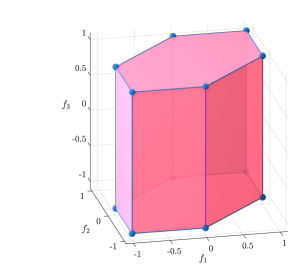
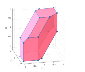
Figure 1. The unit ball $B^{P}_{\mathrm{FM}}$ for the norm $\|\cdot\|_{\mathrm{FM}}$ on the space $\mathrm{BL}(P,d)$, where $P=\{x_{1},x_{2},x_{3}\}$ and $f\in\mathrm{BL}(P,d)$ is represented by $(f_{i})\in\mathbb{R}^{3}$ with $f_{i}:=f(x_{i})$. The defining conditions are given by (36). The metric $d$ is defined by $d_{ij}:=d(x_{i},x_{j})$ and differs for the two cases shown.
Left: $d_{12}=1$, $d_{13}=2$, $d_{23}=3$. Right: $d_{12}=0.75$, $d_{13}=1$, $d_{23}=1.25$.

Write $\tau=\sum_{i=1}^{n}\alpha_{i}\delta_{x_{i}}$ with $0\neq\alpha_{i}\in\mathbb{R}$ and $x_{i}\in S$, and put $P:=\mathrm{supp}(\tau)=\{x_{1},\dots x_{n}\}$. Lemma 1.1 (ii) implies that restriction to $P$ gives a surjective map from $B^{S}_{\mathrm{FM}}$ onto $B^{P}_{\mathrm{FM}}$. Therefore,

(37) $$\|\tau\|_{\mathrm{FM}}^{*}\ =\ \sup_{g\in B^{S}_{\mathrm{FM}}}\langle\tau,g,\rangle\ =\ \sup_{f\in B^{P}_{\mathrm{FM}}}\langle\tau|_{P},f\rangle=\max_{f\in\iota(B^{P}_{\mathrm{FM}})}\ \sum_{i=1}^{n}\alpha_{i}f_{i}.$$

Thus, $\|\tau\|_{\mathrm{FM}}^{*}$ can be computed using one of the many existing – very efficient – optimization algorithms that use linear programming, such as Gurobi and CPLEX, or the built-in ‘linprog’ function in MATLAB, using the standard domain description (36). In these algorithms there is an initial step in which an extreme point of the domain is sought to start the search for the optimum. Here, $\pm(1,\dots,1)$ are always extreme points. If $\sum_{i}\alpha_{i}\geq 0$ one may start at $(1,\dots,1)$. If $\sum_{i}\alpha_{i}<0$,one may start at $(-1,\dots,-1)$. This reduces the number of vertices of $B^{P}_{\mathrm{FM}}$ that needs to be examined by the optimization algorithm in the worst case by a factor two.

Example 5.1.

Let $P=\{x_{1},x_{2},x_{3}\}$ and $d_{12}=1$, $d_{13}=2$ and $d_{23}=3$. Notice that the prescribed distances are consistent with the triangle inequality. Take $\alpha_{1}=1$, $\alpha_{2}=-\mbox{$\frac{1}{3}$}$ and $\alpha_{3}=-\mbox{$\frac{2}{3}$}$. Equation (18) gives an explicit result in this case:

$$\bigl{\|}\sum_{i}\alpha_{i}\delta_{x_{i}}\bigr{\|}_{\mathrm{FM}}^{*}\ =\ |\alpha_{2}|(2\wedge d_{12})+(1-|\alpha_{2}|)(2\wedge d_{13})\ =\ \frac{1}{3}\cdot 1+\frac{2}{3}\cdot 2=\frac{5}{3}.$$

We implemented an algorithm for computing the Fortet-Mourier norms of molecular measures in MATLAB, using the ‘linprog’ algorithm, see Appendix A.2. It returned the same result for the norm, but also an $f$ at which the optimum is attained. In this case $f=(1,0,-1)$. This $f$ corresponds precisely to the function $(-{{1\!\!1}})\vee(1-d(x_{1},\cdot))$ that appears in the theoretical result, Proposition 3.1.

The above linear programming algorithm for computing $\|\tau\|_{\mathrm{FM}}^{*}$ has as domain for the objective function a polygon in $\mathbb{R}^{n}$, where $n$ is the number of points in the support of $\tau\in{\mathcal{M}ol}(S)$. The dimensionality of the optimization problem can be reduced by halve, by resorting to the results of Section 4. The number of points in the support of either $\tau^{+}$ or $\tau^{-}$ is less than $n/2$ or both have precisely $n/2$ points in their support. The one with the least number of points, say $\tau^{-}$ with $N\leq n/2$ points, can play the role of $\nu$ in Section 4, while the other takes up the role of $\mu$, simply because $\|\tau\|_{\mathrm{FM}}^{*}=\|-\tau\|^{*}_{\mathrm{FM}}$.

Thus, with $\nu=\tau^{-}$ (say) and $P=\mathrm{supp}(\nu)=\{x_{1},\dots,x_{N}\}$,

$$\|\tau\|_{\mathrm{FM}}^{*}=\bigl{\|}\tau^{-}-\tau^{+}\bigr{\|}_{\mathrm{FM}}^{*}=\max_{f\in\iota(B^{P}_{\mathrm{FM}})}\psi_{-\tau}(f)=-\min_{f\in\iota(B^{P}_{\mathrm{FM}})}\bigl{(}-\psi_{-\tau}(f)\bigr{)},$$

according to (30) and the further discussion in Section 4. The polygonal domain of optimization $\iota(B^{P}_{\mathrm{FM}})$ is still given by (36), but now has reduced dimension $N\leq n/2$. In this setting, $\psi_{\tau^{-}}$ is ‘linear’ on $\iota(B^{P}_{\mathrm{FM}})$ (Proposition 4.2). If

$$\tau=\sum_{j=1}^{n-N}\beta_{j}\delta_{y_{j}}\ -\ \sum_{i=1}^{N}\alpha_{i}\delta_{x_{i}},\qquad\alpha_{i},\beta_{j}>0,$$

then for $\theta\in\iota(B^{P}_{\mathrm{FM}})$

(38) $$\psi_{-\tau}(\theta)=\sum_{i=1}^{N}\alpha_{i}\theta_{i}-\sum_{j=1}^{n-N}\beta_{j}\bigl{(}(-1)\vee\max_{1\leq i\leq N}(\theta_{i}-d(x_{i},y_{j}))\bigr{)}.$$

So, the reduction in dimension of the domain is to the cost of (part of the) ‘linearity’ of the objective function $-\psi_{-\tau}$ on $\iota(B^{P}_{\mathrm{FM}})$, although it is still convex. Application of one of the existing (efficient) convex optimization algorithms now yields $\|\tau\|_{\mathrm{FM}}^{*}$ on a lower dimensional domain.

6. Computing Dudley norms

So far we have been discussing expressions for and the computation of Fortet-Mourier norms only. The dual bounded Lipschitz norm on ${\mathcal{M}}(S)$, also known as Dudley norm, or flat metric – for the associated metric – is also considered often. It is given by

$$\|\mu\|_{\mathrm{BL}}^{*}:=\sup_{f\in B^{S}_{\mathrm{BL}}}\langle\mu,f\rangle,\qquad B^{S}_{\mathrm{BL}}:=\bigl{\{}f\in\mathrm{BL}(S):\|f\|_{\infty}+|f|_{L}\leq 1\bigr{\}}.$$

The results presented in Section 2 and Section 3 do not readily generalize to the $\|\cdot\|_{\mathrm{BL}}^{*}$-norm. The main issue is, that the geometric shape of $B^{S}_{\mathrm{BL}}$ is more complicated than that of $B^{S}_{\mathrm{FM}}$. For example, we could change the $\|\cdot\|_{\infty}$-norm of a function in $B^{S}_{\mathrm{FM}}$ ‘independently’ from its Lipschitz constant. For $B^{S}_{\mathrm{BL}}$ that is not possible, since the constraint $\|f\|_{\infty}+|f|_{L}\leq 1$ should be maintained.

However, the results of Section 5 can be carried over to the $\|\cdot\|_{\mathrm{BL}}^{*}$-norm. The corresponding statement of (37) is still valid with ‘$\mathrm{FM}$’ replaced by ‘$\mathrm{BL}$’. The description of $\iota(B^{P}_{\mathrm{BL}})$ becomes more awkward though. Without giving the lengthy proof here, we obtained

Lemma 6.1.

Let $n\geq 2$ and $P=\{x_{1},\dots,x_{n}\}\subset S$, consisting of distinct points. Put $d_{ij}:=d(x_{i},x_{j})$. Then

$$\iota(B^{P}_{\mathrm{BL}})\ =\ \bigcap_{1\leq i,j,k\leq n,\ k\neq i\neq j\neq k}\bigl{\{}f_{k}+(f_{i}-f_{j})d_{ij}^{-1}\leq 1\bigr{\}}\cap\bigl{\{}-f_{k}-(f_{i}-f_{j})d_{ij}^{-1}\leq 1\bigr{\}}$$

$$\qquad\cap\ \bigcap_{1\leq i,k\leq n,\ i\neq k}\bigl{\{}f_{k}+(f_{k}-f_{i})d_{ik}^{-1}\leq 1\bigr{\}}\cap\bigl{\{}-f_{k}-(f_{k}-f_{i})d_{ik}^{-1}\leq 1\bigr{\}}.$$

In Figure 2 an example is shown of a unit ball $B^{P}_{\mathrm{BL}}$ for $P$ consisting of three points. Compare the more complex geometric structure with those of $B^{P}_{\mathrm{FM}}$ presented in Figure 1.

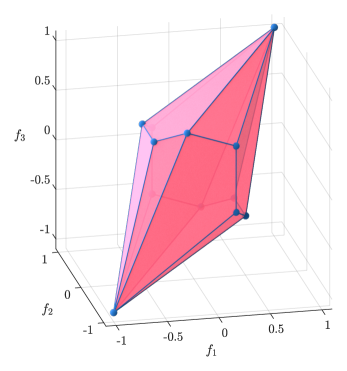
Figure 2. The unit ball $B^{P}_{\mathrm{BL}}$ for the norm $\|\cdot\|_{\mathrm{BL}}$ on the space $\mathrm{BL}(P,d)$, where $P=\{x_{1},x_{2},x_{3}\}$ and $f\in\mathrm{BL}(P,d)$ is represented by $(f_{i})\in\mathbb{R}^{3}$ with $f_{i}:=f(x_{i})$. The defining conditions are given by those in Lemma 6.1, while the metric $d$ is defined by $d_{ij}:=d(x_{i},x_{j})$ with $d_{12}=1$, $d_{13}=2$, $d_{23}=3$.

Thus, one has – with $P$ as in Lemma 6.1 and $0\neq\alpha_{i}\in\mathbb{R}$:

(39) $$\bigl{\|}\sum_{i=1}^{n}\alpha_{i}\delta_{x_{i}}\bigr{\|}_{\mathrm{BL}}^{*}\ =\ \max_{f\in\iota(B^{P}_{\mathrm{BL}})}\sum_{i=1}^{n}\alpha_{i}f_{i}\ =\ -\min_{f\in\iota(B^{P}_{\mathrm{BL}})}\bigl{(}-\sum_{i=1}^{n}\alpha_{i}f_{i}\bigr{)},$$

which optimum can again be found by a linear programming algorithm, now by using Lemma 6.1 for the standard description of the domain of optimization as intersection of half-spaces.

Acknowledgement. We thank M.A. Müller for preparing the graphics showing the unit balls in the spaces of bounded Lipschitz functions over a finite set of points in Figure 1 and Figure 2.

Appendix A MATLAB implementations

A.1. FM-distance between a positive linear combination of Dirac measures and a positive measure

ΨΨ% Computes ||\nu-\mu||_FM^* for \nu in Mol^+(S), \mu in M^+(S),
ΨΨ% S=(Smin, Smax)\subset\R (possibly Smin=-Inf, Smax=+Inf)
ΨΨ% \mu=h d\lambda, \mu abs ct wrt Lebesgue measure, \nu=sum a_i delta_{s_i}
ΨΨ
ΨΨSmin = 0;
ΨΨSmax = Inf;
ΨΨa = [1/2 2 1/5 1/3]; % a=[a_1,...,a_n]
ΨΨn = length(a);
ΨΨP = [0 1/3 1/2 3]; %=supp(\nu)=[s_1,...,s_n]
ΨΨ
ΨΨh = @(s) exp(-s^2);
ΨΨintegrand = @(s,f)h(s)*max(-1,max(f-abs(P-s)));
ΨΨpsi = @(f) -dot(a,f)+integral(@(s) integrand(s,f),Smin,Smax,’ArrayValued’,true);
ΨΨ
ΨΨA = [];
ΨΨfor i = 1:n
ΨΨ    for j = i+1:n
ΨΨ        B = zeros(1,n);
ΨΨ        B(i) = abs(P(i)-P(j))^(-1);
ΨΨ        B(j) = -B(i);
ΨΨ        A = [A;B];
ΨΨ    end
ΨΨend
ΨΨA = [A;eye(n)];
ΨΨA = [A;-A];
ΨΨ
ΨΨb = ones(n^2+n,1);
ΨΨf0 = zeros(1,n);
ΨΨ
ΨΨ[f,val] = fmincon(psi,f0,A,b);
ΨΨf
ΨΨnorm = -val
Ψ

A.2. FM-norm of a linear combination of Dirac measures

ΨΨfunction [norm,f] = FMdualnorm(a,dist)
ΨΨ%a=[a_1 a_2 ... a_n], mu=sum_i=1^n a_i delta_s_i, dist=[d_ij]_i,j=1^n matrix
ΨΨ%norm =||mu||_FM^*, f=ext pt for which <mu,f>=norm
ΨΨn=length(a);
ΨΨA=[];
ΨΨfor i=1:n
ΨΨ    for j=i+1:n
ΨΨ        B=zeros(1,n);
ΨΨ        B(i)=dist(i,j)^(-1);
ΨΨ        B(j)=-B(i);
ΨΨ        A=[A;B];
ΨΨ    end
ΨΨend
ΨΨA=[A;eye(n)];
ΨΨA=[A;-A];
ΨΨb=ones(n^2+n,1); %m=#rows of A=2n+2(n choose 2)=2n+n(n-1)=n^2+n
ΨΨminus_a=-a;
ΨΨf=linprog(minus_a,A,b);
ΨΨnorm=a*f;
Ψ

References

[1] Ackleh, A.S., D.F. Marshall, H.E. Heatherly and B.G. Fitzpatrick (1999). Survival of the fittest in a generalized logistic model, Math. Models Methods Appl. Sci.9(9), pp. 1379–1391.
[2] Ackleh, A.S., B.G. Fitzpatrick and H.R. Thieme (2005). Rate distributions and survival of the fittest: a formulation on the space of measures, Discr. Contin. Dyn. Syst. Ser. B5(4), pp. 917–928.
[3] Ackleh, A.S., N. Saintier and J. Skrzeczkowski (2019). Sensitivity equations for measure-valued solutions of transport equations, Math. Biosci. Engineering17(1), pp. 514–537.
[4] Alkurdi, T., S.C. Hille and O. van Gaans (2013). Ergodicity and stability of a dynamical system perturbed by impulsive random interventions. J. Math. An. Appl.63, pp. 480–494.
[5] Bačák, M. (2014). Convex analysis and optimization in Hadamard spaces, Vol. 22, De Gruyter.
[7] Bertsimas, D. (1997). Introduction to linear optimization, Athena Scientific, Belmont.
[8] Bogachev, V.I. (2007). Measure Theory, Volume II, Springer-Verlag, Berlin-Heidelberg.
[9] Boyd, S. and L. VandenBerghe (2004). Convex optimization, Cambridge University Press.
[10] Carillo, J.A., R.M. Colombo, P. Gwiazda and A. Ulikowska (2012). Structured populations, cell growth and balance laws, J. Diff. Equ.252, pp. 3245–3277.
[11] Church, R.L., Z. Drezner and A. Tamir (2022). Extensions to the Weber problem, Comput. Oper. Res.143, p. 105786.
[12] Cottet, G.H. and S. Mas-Gallic (1990). A particle method to solve the Navier-Stokes system, Numer. Math.57, pp. 805–827.
[13] Czapla, D., S.C. Hille, K. Horbacz and H. Wodjewódka-Ścia̧żko (2019). Continuous dependence of an invariant measure on the jump rate of a piecewise-deterministic Markov process, Math. Biosci. Engineering17(2), pp. 1059–1073.
[14] Deutsch, F. (1980). Existence of best approximations, J. Approx. Theory28(2), pp. 132–154.
[15] Dolbeault, J. and C. Schmeiser (2009). The two-dimensional Keller-Segel model after blow-up, Discrete Contin. Dyn. Syst.25(1), pp. 109-121.
[16] Drezner, Z., K. Klamroth, A. Schöbel and G.O. Wesolowsky (2002). The Weber problem. In Facility location, Springer-Verlag, pp. 1–36.
[17] Dudley, R. (1966). Convergence of Baire measures, Studia Math.27(3), pp. 251–268.
[18] Evers, J.H.M. (2015). Evolution equations for systems governed by social interactions, PhD thesis, Technische Universiteit Eindhoven.
[19] Evers, J.H.M., S.C. Hille and A. Muntean (2016). Measure-valued mass evolution problems with flux boundary conditions and solution-dependent velocities, SIAM J. Math. Anal.48(3), pp. 1929–1953.
[20] Gwiazda, P., S.C. Hille, K. Lyczek and A. Swierczewska-Gwiazda (2019). Differentiability in perturbation parameter of measure solutions to perturbed transport equation, Kinetic and Related Models17(2), pp. 1093–1108.
[21] Herrero, A. and J.J.L. Velázquez (1997). A blow-up mechanism for a chemotaxis model, Ann. Sc. Norm. Super. Pisa Cl. Sci.24(4), pp. 633–683.
[22] Hille, S.C., K. Horbacz and T. Szarek (2016). Existence of a unique invariant measure for a class of equicontinuous Markov operators with application to a stochastic model for an autoregulated gene, Annales Mathématiques Blaise Pascal23(2), pp. 171–217.
[23] Hille, S.C. and D.T.H. Worm (2009). Embedding of semigroups of Lipschitz maps into positive linear semigroups on ordered Banach spaces generated by measures, Integral Equ. Oper. Theory63(3), pp. 351–371.
[24] Jabłoński, J. and A. Marciniak-Czochra (2013), Efficient algorithms computing distances between Radon measures on , ArXiv preprint.
[25] Kuhn, H.W. and R.E. Kuenne (1962). An efficient algorithm for the numerical solution of the generalized Weber problem in spatial economics, J. Reg. Sci.4(2), pp. 21–33.
[26] Lasota, A. and J. Myjak (1999). Fractals, semifractals and Markov operators, Int. J. Bif. Chaos9(2), pp. 307–325.
[27] Lasota, A., J. Myjak and T. Szarek (2002). Markov operators with a unique invariant measure, J. Math. Anal. Appl.276, pp. 343–356.
[28] McShane, E.J. (1934). Extension of range of functions, Bull. Am. Math. Soc.40, pp. 837-–842.
[29] Pachl, J. (2013). Uniform spaces and measures, Fields Institute Monographs, Volume 30, The Fields Institute for Research in the Mathematical Sciences, Springer, New York.
[30] Piccoli, B. and F. Rossi (2014). Generalized Wasserstein distance and its application to transport equations with source, Arch. Rational Mech. Anal.211, pp. 335–358.
[31] Piccoli, B. F. Rossi and M. Tournus (2021). A Wasserstein norm for signed measures, with application to a non local transport equation with source term, HAL preprint. hal-01665244v5
[32] Piccoli, B. and A. Tosin (2011). Time-evolving measures and macroscopic modeling of pedestrian flow, Arch. Rational Mech. Anal.199, pp. 707–738.
[33] Rockafellar, R.T. (1972). Convex analysis, Princeton University Press.
[34] Sriperumbudur, B.K., K. Fukumizu, A. Gretton, B. Schölkopf and G.R.G Lanckriet (2012). On the empirical estimation of integral probability metrics, Electr. J. Stat.6, pp. 1550–1599.
[35] Villani, C. (2003). Topics in Optimal Transportation, American Mathematical Society, Providence.