Reinforcement learning based adaptive metaheuristics

Abstract.

Parameter adaptation, that is the capability to automatically adjust an algorithm’s hyperparameters depending on the problem being faced, is one of the main trends in evolutionary computation applied to numerical optimization. While several handcrafted adaptation policies have been proposed over the years to address this problem, only few attempts have been done so far at applying machine learning to learn such policies. Here, we introduce a general-purpose framework for performing parameter adaptation in continuous-domain metaheuristics based on state-of-the-art reinforcement learning algorithms. We demonstrate the applicability of this framework on two algorithms, namely Covariance Matrix Adaptation Evolution Strategies (CMA-ES) and Differential Evolution (DE), for which we learn, respectively, adaptation policies for the step-size (for CMA-ES), and the scale factor and crossover rate (for DE). We train these policies on a set of 46 benchmark functions at different dimensionalities, with various inputs to the policies, in two settings: one policy per function, and one global policy for all functions. Compared, respectively, to the Cumulative Step-size Adaptation (CSA) policy and to two well-known adaptive DE variants (iDE and jDE), our policies are able to produce competitive results in the majority of cases, especially in the case of DE.

1. Introduction

One of the key reasons for the success of metaheuristics is their being general-purposeness. Indeed, Evolutionary Algorithms (EAs), Swarm Intelligence (SI) algorithms and alike can be applied, more or less straightforwardly, to a broad range of optimization problems. On the other hand, it is well-established that different algorithms can produce different results on a given problem, and in fact it is impossible to identify an algorithm that works better than any other algorithm on all possible problems (Wolpert and Macready, 1997).

Moreover, the performance of metaheuristics typically depends on their hyper-parameters. However, optimal parameters are usually problem-dependent, and finding those parameters before performing an optimization process through trial-and-error or other empirical approaches is usually tedious, and obviously suboptimal. One possible alternative is given by hyperheuristics (Burke et al., 2013; Drake et al., 2020; Sánchez et al., 2020), i.e., algorithms that can either select the best metaheuristic for a given problem (Nareyek, 2003; Chakhlevitch and Cowling, 2008; Li et al., 2017), or simply optimize the parameters of a given metaheuristic. Several tools, e.g. irace (López-Ibáñez et al., 2016), exist for this purpose.

Another possibility is to endow the metaheuristic with a parameter adaptation strategy, i.e., a set or rules that change the parameters dynamically during the optimization process. Several handcrafted, successful policies have been proposed over the years to address parameter adaptation (Cotta et al., 2008). However, finding an optimal adaptation policy is, in turn, challenging as different policies may perform differently on different problems or during different stages of an optimization process. Moreover, exploring manually the space of such policies is infeasible. On the other hand, it is possible to cast the search for an adaptation policy as a reinforcement learning (RL) problem (Sutton and Barto, 2018), where the agent observes the state of the optimization process and decides how to change the parameters accordingly. However, only few attempts have been done so far in this direction. This is mostly due to the fact that the observation space of an optimization process can be quite large, and finding relevant state metrics (i.e., inputs to the policy) and rewards can be difficult.

Here, we aim to make steps in this direction by introducing a general-purpose framework for performing parameter adaptation in continuous-domain metaheuristics based on state-of-the-art RL. One reason for building such a framework is to relieve algorithm designers and practitioners from the need for building handcrafted adaptation strategies. Moreover, using such framework would allow to use pretrained strategies and apply them to new optimization problems.

In the experimentation, we focus on two well-known continuous optimization algorithms (assuming, without loss of generalization, minimization of the objective function/fitness), namely the Covariance Matrix Adaptation Evolution Strategies (CMA-ES) (Hansen and Ostermeier, 2001) and Differential Evolution (DE) (Storn and Price, 1997), for which well-known successful handmade adaptation policies exist. In the case of CMA-ES, we train an adaptation policy for the step-size $\sigma$. In the case of DE, we instead adapt the scale factor $F$ and the crossover rate $CR$. We train these policies on a set of 46 benchmark functions at different dimensionalities, with various state metrics, in two settings: one policy per function, and one global policy for all functions. Compared, respectively, to the Cumulative Step-size Adaptation (CSA) policy (Chotard et al., 2012) and to two well-known adaptive DE variants (iDE (Elsayed et al., 2011) and jDE (Brest et al., 2006)), our policies are able to produce competitive results, especially in the case of DE.

The rest of the papers is structured as follows. In the next section, we briefly present the related works. In Section 3, we describe our methods. In Section 4, we then present our results. Finally, we draw the conclusions in Section 5.

2. Background

In the context of DE, several works have shown the effect of using an adaption strategy to choose $F$ and $CR$. These parameters are, in fact, known to affect both diversity and optimization results (Yaman et al., 2019). For instance, some authors proposed using pools of different parameters and mutation/crossover strategies, either as discrete sets of fixed values (Iacca et al., 2014), or as continuous ranges (Iacca et al., 2015). Others proposed using multiple mutation strategies (Yaman et al., 2018), where each strategy is represented as an agent whose measured performance is used to promote its activation within an ensemble of strategies. Recently, the authors of (Julian Blank, 2022) introduced a polynomial mutation for DE with different approaches for controlling its parameter. The authors of (Ghosh et al., 2022) proposed instead an improvement on SHADE (Tanabe and Fukunaga, 2013), which uses proximity-based local information to control the parameter settings.

Rather than engineering the parameter adaptation strategy, some studies have tried to learn metaheuristics with RL. Some of these works are based on Q-learning: Li et al. (Li et al., 2019) considered each individual as an agent that learns the optimal strategy for solving a multi-objective problem with DE; in a similar way, Hu et al. (Hu et al., 2021) used a Q-table for each individual to choose how much to increase/decrease the $F$ parameter during a DE run to solve circuit design problems; Sallam et al. (Sallam et al., 2020) proposed an algorithm that evolves two populations: one with CMA-ES, and one with Q-table, in order to choose between different DE operators and enhance the EA with a local search.

Other approaches are based on deep RL: Sharma et al. (Sharma et al., 2019) proposed a method that uses deep RL that produces an adaptive DE strategy based on the observation of several state metrics; Sun et al. (Sun et al., 2021) trained a Long-Short Term Memory (LSTM) with policy gradient to control the $F$ and $CR$ parameters in DE; Shala et al. (Shala et al., 2020) trained a neural network with Guided Policy Search (GPS) (Levine and Koltun, 2013) to control the step-size of CMA-ES by also sampling trajectories created by Cumulative Step-size Adaptation (CSA) (Chotard et al., 2012); Lacerda et al. (LACERDA, 2021) used distributed RL to train several metaheuristics with Twin Delayed Deep Deterministic Policy Gradients (Fujimoto et al., 2018).

3. Methods

The proposed framework uses deep RL to learn parameter adaptation strategies for EAs, i.e., to learn a policy that is able to set the parameters of an EA at each generation of the optimization process. In that, our framework is similar to the approach presented in (Shala et al., 2020). However, differently from (Shala et al., 2020) we do not use GPS as RL algorithm and, most importantly, we do not partially sample the parameter adaptation trajectory from an existing adaptation strategy (in (Shala et al., 2020), CSA), but rather we build the adaptation trajectory from scratch, i.e., entirely based on the trained policy. Another important aspect is that our framework can be configured with different EAs and RL algorithms, and can be easily extended in terms of state metrics, actions and rewards.

Next, we briefly describe the two EAs considered in our experimentation (Section 3.1), the RL setting (Section 3.2), the evaluation procedure (Section 3.3) and the computational setup (Section 3.4).

3.1. Evolutionary algorithms

We tested the framework using CMA-ES and DE since these are two well-known EAs for which several studies exist on parameter adaptation. In our comparisons, we considered two well-established adaptation strategies taken from the literature: for CMA-ES, Cumulative Step-size Adaptation (CSA) (Chotard et al., 2012); for DE, iDE (Elsayed et al., 2011) and jDE (Brest et al., 2006). More details on these adaptation strategies will follow.

3.1.1. Covariance Matrix Adaptation Evolution Strategies

CMA-ES (Hansen and Ostermeier, 2001) conducts the search by sampling adaptive mutations from a multivariate normal distribution ($x_{i}\sim\boldsymbol{m}+\sigma\times\mathcal{N}(0,\boldsymbol{C})$). At each generation, the mean $\boldsymbol{m}$ is updated based on a weighted average over the population, while the covariance matrix $\boldsymbol{C}$ is updated by applying a process similar to that of Principle Component Analysis. The remaining parameter, $\sigma$ is the step size, which in turn is adapted during the process. Usually, $\sigma$ is self-adapted using CSA (Chotard et al., 2012). In our case, the policy is learned and computed based on an observation of the current state of the search.

3.1.2. Differential Evolution

DE (Storn and Price, 1997) is a very simple yet efficient EA. Starting from an initial random population, at each generation the algorithm applies on each parent solution a differential mutation operator, to obtain a mutant, which is then crossed over with the parent. While there are different mutation and crossover strategies for DE, in this study we consider only the “best/1/bin” strategy. According to this strategy, the mutant is computed as $\boldsymbol{x}^{k+1}=\boldsymbol{x}^{k}_{best}+F\times(\boldsymbol{a}-\boldsymbol{b})$; where $\boldsymbol{x}^{k}_{best}$ is the best individual at the $k$-th generation, $\boldsymbol{a}$ and $\boldsymbol{b}$ are two mutually exclusive randomly selected individuals in the current population, and $F$ is the scale factor. The binary crossover, on the other hand, swaps the genes of parent and mutant with probability given by the crossover rate $CR$.

Without adaptation, $F$ and $CR$ are fixed. In our case, we make the policy learn how to adapt them by using two different approaches: directly updating $F$ and $CR$ with the policy, or sampling $F$ and $CR$ from a uniform/normal distribution parametrized by the policy.

3.2. Reinforcement learning setting

As for the RL setting, we chose the same model used in (Shala et al., 2020): 2 fully connected hidden layers of 50 neurons each (thus with $50\times 50$ connections) with ReLU activation function. The size if the input layer depends on the observation space, while the size of the output layer depends on the action space. In the following, we describe the other details of the learning setting.

3.2.1. Proximal Policy Optimization

We chose Proximal Policy Optimization (PPO) (Schulman et al., 2017) to optimize the policy due to its good performances in general-purpose RL tasks. Here, for brevity we do not go into details of the algorithm (for which we refer to (Schulman et al., 2017)), but in short the algorithm works as shown in Algorithm 1.

In our setup, $N=1$, $K=200$, and the other parameters are set as per their defaults value used in the ray-rllib library. $\theta$ are the parameters of the policy (in our case, the weights of the neural networks), $L$ is the loss function (see Eq. 9 from (Schulman et al., 2017)) and $\hat{A}_{t}$ is the advantage estimate at iteration $t$ (see Eq. 11 from (Schulman et al., 2017)).

3.2.2. Observation spaces

We experimented with different observation spaces, each one defined as a set of state metrics. A state metric computes the state (or observation) of the model based on various combinations of fitness values, genotypes, and other parameters of the EA. More specifically, we used the following state metrics:

• Inter-generational $\Delta f$: For the last $g$ generations, we take the best fitness in the population at each generation and compute the normalized difference with the best fitness at the previous generation:

  (1) $$\Delta f^{inter}_{g}=\Big{[}\Delta f^{inter}_{k},\Delta f^{inter}_{k-1},\dots,\Delta f^{inter}_{k-(g-1)}\Big{]}$$

  (2) $$\text{where}\quad\Delta f^{inter}_{k}=\frac{f^{*}_{k}-f^{*}_{k-1}}{|f^{*}_{k}-f^{*}_{k-1}|+|f^{*}_{k-1}|+10^{-5}}$$

  where $f^{*}_{k}$ is the best fitness value in the population at the $k$-th generation. In this way, $\Delta f^{inter}_{k}\in(-1,1)$ and it is proportional to the best fitness from the previous generation, saturating to $\pm 1$ for $f^{*}_{k}\rightarrow\pm\infty$. The constant $10^{-5}$ is needed to avoid divisions by zero. The normalization of $\Delta f$ is fundamental to have stable training.

• Intra-generational $\Delta f$: For the last $g$ generations, we take the normalized difference between the maximum and minimum fitness of the current population at each generation:

  (3) $$\Delta f^{intra}_{k}=\frac{|f^{max}_{k}-f^{min}_{k}|}{|f^{max}_{k}-f^{min}_{k}|+|f^{*}_{k}|+10^{-5}}.$$

• Inter-generational $\Delta\boldsymbol{X}$: Similarly to the inter-generational $\Delta f$, the normalized difference between the best genotype in two consecutive generations are taken for the last $g$ generations. In this case, to maintain linearity, the normalization is done using the bounds of the search space:

  (4) $$\Delta\boldsymbol{X}^{inter}_{k}=\frac{\boldsymbol{X}^{*}_{k}-\boldsymbol{X}^{*}_{k-1}}{\Delta\boldsymbol{X}^{bounds}}$$

  where $\boldsymbol{X}^{*}_{k}$ is the genotype associated to the best fitness at generation $k$ and $\Delta\boldsymbol{X}^{bounds}=\Big{[}\Delta\boldsymbol{X}^{bounds}_{1},\dots,\Delta\boldsymbol{X}^{bounds}_{d}\Big{]}$ is the vector containing, for each variable, the bounds of the search space, being $d$ the problem size. Since the size of this observation would depend on the problem size, the policy would work only with problems of that fixed size. To solve this problem, we use as observation the minimum and maximum values of $\Delta\boldsymbol{X}^{inter}_{k}$:

  (5) $$\Delta\boldsymbol{X}^{inter}_{k_{min,max}}=\Big{[}\min(\Delta\boldsymbol{X}^{inter}_{k}),\max(\Delta\boldsymbol{X}^{inter}_{k})\Big{]}.$$

  The intra-generational $\Delta\boldsymbol{X}$ is then defined as a history of the above defined metric at the last $g$ generations:

  (6) $$\Delta\boldsymbol{X}^{inter}=\Big{[}\Delta\boldsymbol{X}^{inter}_{k_{min,max}},\Delta\boldsymbol{X}^{inter}_{k-1_{min,max}},\dots,\Delta\boldsymbol{X}^{inter}_{k-(g-1)_{min,max}}\Big{]}.$$

• Intra-generational $\Delta\boldsymbol{X}$: Given $\boldsymbol{X}^{k}_{i_{j}}$ as the $j$-th dimension of the $i$-th individual of the population at the $k$-th generation, the intra-generational $\Delta\boldsymbol{X}$ at the $k$-th generation is defined as:

  (7) $$\Delta\boldsymbol{X}^{intra}_{k}=\Big{[}\boldsymbol{X}^{intra}_{k_{1}},\dots,\boldsymbol{X}^{intra}_{k_{d}}\Big{]}$$

  (8) $$\text{where}\quad\Delta\boldsymbol{X}^{intra}_{k_{j}}=\frac{\left|\boldsymbol{X}^{k}_{max_{j}}-\boldsymbol{X}^{k}_{min_{j}}\right|}{\Delta\boldsymbol{X}^{bounds}_{j}}.$$

  Also in this case, we use as observation the minimum and maximum values of $\Delta\boldsymbol{X}^{intra}_{k}$:

  (9) $$\Delta\boldsymbol{X}^{intra}_{k_{min,max}}=\Big{[}\min(\Delta\boldsymbol{X}^{intra}_{k}),\max(\Delta\boldsymbol{X}^{intra}_{k})\Big{]}.$$

  The intra-generational $\Delta\boldsymbol{X}$ is then defined as a history of the above defined metric at the last $g$ generations:

  (10) $$\Delta\boldsymbol{X}^{intra}=\Big{[}\Delta\boldsymbol{X}^{intra}_{k_{min,max}},\Delta\boldsymbol{X}^{intra}_{k-1_{min,max}},\dots,\Delta\boldsymbol{X}^{intra}_{k-(g-1)_{min,max}}\Big{]}.$$

In all the experiments, we always include in the observation space also the previous model output, i.e., the parameters given by the model in the previous generation.

1 for iteration = $1,2,\dots I$ do

2       for actor = $1,2,\dots N$ do

3             Run policy $\pi_{\theta_{old}}$ in environment for $T$ timesteps

4             Compute advantage estimates $\hat{A}_{1},\dots,\hat{A}_{T}$

5       end for

6      Optimize loss $L$ w.r.t. $\theta$, with $K$ epochs and minibatch size $M\leq N\times T$

7       $\theta_{old}\leftarrow\theta$

8 end for

Algorithm 1 High-level description of PPO.

3.2.3. Action spaces

The action space of the policy depends on both the specific EA and the approach used to parametrize it. In our model, the action is taken at every generation, using the observation from the previous one. In our experiments, we considered the following action spaces:

• CMA-ES (Step-size): $\sigma\in[10^{-10},3]$.

• DE (Both $F$ and $CR$): $F\in[0,2],CR\in[0,1]$.

• DE (Normal distribution): $F$ and $CR$ are sampled using two normal distributions parametrized with mean and standard deviation determined by the learned policy, i.e., respectively, $\mathcal{N}(\mu_{F},\sigma_{F})$ and $\mathcal{N}(\mu_{C}R,\sigma_{C}R)$. Thus, the action space is: $\Big{\{}\mu_{F}\in[0,2]$, $\sigma_{F}\in[0,1]$, $\mu_{CR}\in[0,1]$, $\sigma_{CR}\in[0,1]\Big{\}}$.

• DE (uniform distribution): $F$ and $CR$ are sampled using two uniform distributions parametrized with lower and upper bound determined by the learned policy, i.e., respectively, $\mathcal{U}(F_{min},F_{max})$ and $\mathcal{U}(CR_{min},CR_{max})$. Thus, the action space is: $\Big{\{}F_{min}\in[0,2]$, $F_{max}\in[0,2],CR_{min}\in[0,1],CR_{max}\in[0,1]\Big{\}}$.

3.2.4. Reward

The reward is a scalar representing how good or bad was the performance of the policy during the training episodes (in our case, an episode is a full evolutionary run). It is computed every generation using the Inter-generational $\Delta f$ without history, see Eq. (2). The use of this reward brings some advantages: it reflects the progress of the optimization process, maintaining the independence with different scales of the objective functions, and it yields better numerical stability during the training process. All the experiments have been done using this reward function (except the one presented in Section 4.1.1).

3.2.5. Training procedure

We consider two policy configurations: single-function policy, and multi-function policy. In the first configuration, the model is trained separately on each function: in this way, the policy specializes for each single optimization problem. If the ideal policy should work well on as many functions as possible, a single-function policy can be useful to get an idea about the top performance that the policy can get for each function. Or, single-function policies could used for similar functions. In the second configuration, the model is instead trained using the evolutionary runs on multiple functions. Quite surprisingly, with this procedure, we could obtain policies that are able to work better than the adaptive approaches from the literature.

In all our experiments, we trained the models for $5000$ function evolutionary runs (i.e., episodes), each consisting of $500$ function evaluations, hence meaning $2.5\times 10^{6}$ function evaluations per each policy training. Then, the trained policy is tested using the procedure defined in Section 3.3.4.

3.3. Evaluation

3.3.1. Benchmark functions

The experiments have been done with 46 benchmark functions taken from the BBOB benchmark (Finck et al., 2010). For each function, we used the default instance, i.e., without random shift in the domain or codomain (as done in (Shala et al., 2020)). Future investigations will extend the analysis to instances with shift.

The 46 functions are selected as follows. The first 10 functions are: BentCigar, Discus, Ellipsoid, Katsuura, Rastrigin, Rosenbrock, Schaffers, Schwefel, Sphere, Weierstrass, all in 10 dimensions. The remaining 36 functions are the same 12 functions, namely: AttractiveSector, BuecheRastrigin, CompositeGR, DifferentPowers, LinearSlope, SharpRidge, StepEllipsoidal, RosenbrockRotated, SchaffersIllConditioned, LunacekBiR, GG101me, and GG21hi, each one in 5, 10 and 20 dimensions.

3.3.2. Compared methods

We compared the learned policies with the following adaptive methods from the literature:

1. Cumulative Step-size adaptation (Chotard et al., 2012): CSA is considered the default step-size control method of CMA-ES. To compute $\sigma_{t+1}$, a cumulative path is defined as: $\boldsymbol{p}_{t+1}=(1-c)\boldsymbol{p}_{t}+\sqrt{c(2-c)}\boldsymbol{\xi}^{*}_{t}$, where $c\in[0,1]$ ($1/c$ represents the lifespan of the information contained in $\boldsymbol{p}_{t}$) and $\boldsymbol{\xi}^{*}_{t}$ is the best children at the $t$-th generation. The step-size is defined as: $\sigma_{t+1}=\sigma_{t}exp(\frac{c}{d_{\sigma}}(\frac{||\boldsymbol{p}_{t+1}||}{E(||\mathcal{N}(0,I_{n})||)}-1))$, where $d_{\sigma}$ is the damping parameter that determines how much the step size can change (usually, $d_{\sigma}=1$).

2. iDE (Elsayed et al., 2011): The iDE adaptive method maintains a different $F$ and $CR$ for each individual and updates them with a different rule that depends on the mutation/crossover strategy used. Since in our DE experiments we use the best/1/bin strategy, the considered iDE update rules are:

   (11) $$F=F_{best}+\mathcal{N}(0,0.5)\cdot(F_{r_{1}}-F_{r_{2}})$$

   (12) $$CR=CR_{best}+\mathcal{N}(0,0.5)\cdot(CR_{r_{1}}-CR_{r_{2}})$$

   where $F_{best}$ and $CR_{best}$ are the $F$ and $CR$ values corresponding to the best individual and $F_{r_{i}}$ (or $CR_{r_{i}}$) is a random $F$ (or $CR$) sampled from the best $F$ (or $CR$) values until the current generation ($i$ is needed to selected mutually exclusive values for each individual).

3. jDE (Brest et al., 2006): jDE is a simple but effective adaptive DE variant. With probability $p=0.1$ the method samples $F$ from $\mathcal{U}(0.1,1)$. Otherwise, it uses the best $F$ until the current generation.

3.3.3. Evaluation metrics

In order to compare the different setups of algorithms and models, we consider two metrics (similar to (Shala et al., 2020)):

• Area Under the Curve (AUC): During each evolutionary run, the minimum fitness of the population at each generation is stored. The result is a monotonic non-increasing discrete function (assuming elitism). The area under this curve is then calculated using the composite trapezoidal rule. This metric is a good indication of how fast the optimization process is.

• Best of Run: The best fitness found during the entire optimization process.

As we assume minimization of the objective function, for both metrics it holds that the lower their values, the better is the performance of a policy.

3.3.4. Testing procedure

Given a RL based trained policy $\pi_{A}$ and an adaptive policy $\pi_{B}$ taken from the literature (e.g., CSA) that take actions on the corresponding EA (e.g., CMA-ES), the two policies are tested in the following way:

1. We take the policy $\pi_{A}$ and execute 50 runs, each one for 50 generations, with a population of 10 individuals. Thus, every run has 500 function evaluations.

2. We do the same for policy $\pi_{B}$.

3. For each run of both policies, we compute the two metrics (AUC and Best of Run).

4. For both metrics, we calculate the probability that $\pi_{A}$ performs better than $\pi_{B}$ as:

   (13) $$p(\pi_{A}<\pi_{B})=\frac{1}{n^{2}}\sum_{i}^{n}\sum_{j}^{n}\mathbb{1}_{\pi_{A_{i}}<\pi_{B_{j}}}$$

   where $\mathbb{1}_{\pi_{A_{i}}<\pi_{B_{j}}}$ is 1 if the metric of $\pi_{A}$ on the $i$-th run is less than the metric of $\pi_{B}$ on the $j$-th run, otherwise it is 0.

3.4. Computational setup

We ran our experiments on an Azure Virtual Machine with an 8 core 64-bit CPU (we noted that the CPU model would change over different sessions, but usually the machine used an Intel Xeon with $>$2GHz and $>$30MB cache) and 16GB RAM, running Ubuntu 20.04. A training process of $5000$ episodes takes $\sim 1-1.5$ hours.

Our code is implemented in python (v3.8) using ray-rllib (v1.7), gym (v0.19) and numpy (v1.19). We took the CSA implementation from the cma (v3.1.1) library, as well as the BBOB benchmark functions (Finck et al., 2010). The implementation of DE was done by slightly modifying the scipy’s implementation in order to make it compatible with $F$ and $CR$ at the individual level. The implementation of iDE and jDE has been realized by porting it from the C++ implementation available in the pagmo (v2.18.0) library (that is based on the algorithm descriptions presented in (Elsayed et al., 2011) and (Brest et al., 2006)).

4. Results

We now present the results, separating the experiments with CMA-ES (Section 4.1) from those with DE (Section 4.2).

4.1. CMA-ES experiments

4.1.1. Comparison between PPO and GPS

The first experiment was done with CMA-ES and single-function training, trying to configure the model as similarly as possible to (Shala et al., 2020), in order to get a first comparative analysis. However, a direct comparison with the results reported in (Shala et al., 2020) was not possible. In fact, the authors of (Shala et al., 2020) used GPS as training algorithm, that is not implemented in the ray-rllib library. To avoid replicability issues, we then decided to train our model using the available PPO implementation from ray-rllib. Furthermore, we did not use the sampling rate technique implemented in (Shala et al., 2020), i.e., in our case the trajectories of the step-size are taken entirely from the trained policy.

The rest of the setup is the same used in (Shala et al., 2020). As mentioned earlier, we used 2 fully connected hidden layers of 50 neurons each with ReLU. The observation space is: differences between successive fitnesses from 40 previous generations (not normalized), the step-size history from 40 previous generations, the current cumulative path length (Equation 2 from (Shala et al., 2020)). The reward is the negative of the fitness (not normalized). The action space is $\sigma\in[0.05,3]$. Please note that these state metrics and reward are different from the ones described in Section 3.2, and have been used only in this preliminary experiment for comparison with the results from (Shala et al., 2020).

We performed this experiment only with the first 10 functions of the considered benchmark. The result of this experiment was quite poor: the single-function trained policy obtained better testing results than CSA ($p(\pi<CSA)$ with both AUC and Best of Run metrics) only on 2 functions. We found that the main reason for this scarce performance is the noisy reward. In fact we observed that, depending on the function, the scale of the fitness differs across multiple runs, and PPO is sensible to the reward scale. This seems to explain why the authors of (Shala et al., 2020) chose GPS, which is robust to different reward scales.

Also, with this setup we encountered numerical instability problems: with BentCigar, Rosenbrock and Schaffers we have not been able to train the policy because at a certain point of the training process the weights of the model became NaN. This is very likely caused by the noisy reward, which makes some gradient or loss function value go to infinity. Indeed, this problem was almost totally fixed using a normalized reward.

4.1.2. Normalizing the reward

We tried to improve the previous setup by normalizing the reward and using a minimal observation space. The reward in this case is the one explained in Section 3.2.4. The observation space is the inter-generational $\Delta f$ with $g=40$ and the step-size of the previous generation. Testing the policy on all the 46 functions, it did better than CSA on 30.4% (14/46) of the functions. Moreover, we did not have training stability issues. Overall, we found that CSA is a very good step-size adaptation strategy and it is difficult to do better by means of RL.

4.2. DE experiments

A more intensive experimentation has been conducted with DE. We started with single-function training policies, training one model per function. Then we experimented with multi-function training, applying small changes in the model in order to get close to the single-function results.

4.2.1. Single-function policy

In Figure 1 we report the results of the single-function training policies using three action spaces to parametrize DE, and compare them with iDE and jDE. For brevity, we report only the results of the Best of Run metric. Green (red) cells indicate that the trained policy $\pi$ works better (worse) than the corresponding adaptive DE variant (thus, either iDE or jDE), with $\pi$ trained separately and tested on each function. Darker green (red) indicates higher (lower) probabilities. Black cells indicate that the policy could not be trained due to numerical instability issues: in fact DE, due to its random nature, is likely to produce different fitness trajectories across evolutionary runs. This causes a noisy reward that can lead to numerical instabilities during the training process.

To solve this problem, it is necessary to design a custom loss function for the training algorithm. However, this would mean to use a variation of PPO, which falls outside the scope of this work where we are limiting ourselves to using the original PPO. A simple workaround was to run the training process multiple times: in most cases, one or two attempts were enough to train the policy without encounter this instability problem. Moreover, we observed that using the hyperbolic tangent as activation function (instead of ReLu) can help reduce the probability to encounter instabilities. However, we did not perform a deeper analysis on this.

The leftmost side of Figure 1 shows the percentage of the functions where the learned policy did better than iDE/jDE over the total number of functions: $ratio=\frac{||p(\pi_{i}<iDE/jDE)>0.5||}{n_{functions}}$. It can be seen that the uniform distribution strategy gives the best results overall. However, there are a few functions where the adaptive strategies provided by iDE and jDE always do better.

4.2.2. Multi-function policy

After seeing the results of the normal and uniform distribution approaches in the single-function setting, we experimented with multi-function training using one policy trained for $5000$ episodes on all the $46$ functions, meaning $\sim 108$ evolutionary runs per function. We trained and compared 9 versions of the model with different observation spaces combining the state metrics defined in Section 3.2.2.

The results of this experiment are shown in Figure 2. All the policies have at least the inter-generational $\Delta f$ and the values of the precedent action as observation. The entries on the rightmost side of Figure 2 (starting with “w/”) denote what is included in the observation space. Moreover, we also tried to double the number of training episodes (“double training” labels) and increase the size of the model to $100\times 50\times 10$ (“bigger net” label).

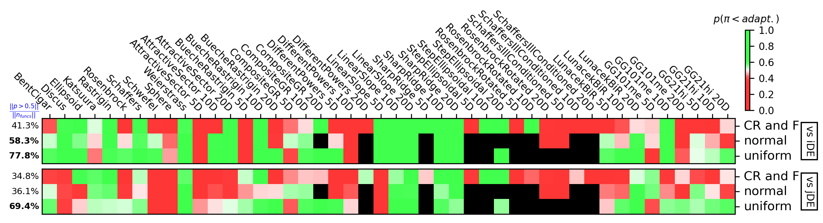
Figure 1. Single-function training policies compared with iDE (top) and jDE (bottom). The color is based on $p(\pi<adapt.)$, see Eq. (13), calculated on the “Best of Run” metric, where $\pi$ is the policy trained separately and tested on each function, and “adapt.” is either iDE or jDE. Black cells indicate that the model has not been trained due to numerical instability. Green (red) cells indicate that the trained policy $\pi$ works better (worse) than the corresponding adaptive DE variant. Darker green (red) indicates higher (lower) probabilities. Percentages on the left side of the rows are calculated as $\frac{\text{no. green cells}}{\text{no. green cells+no. red cells}}$ on the same row.

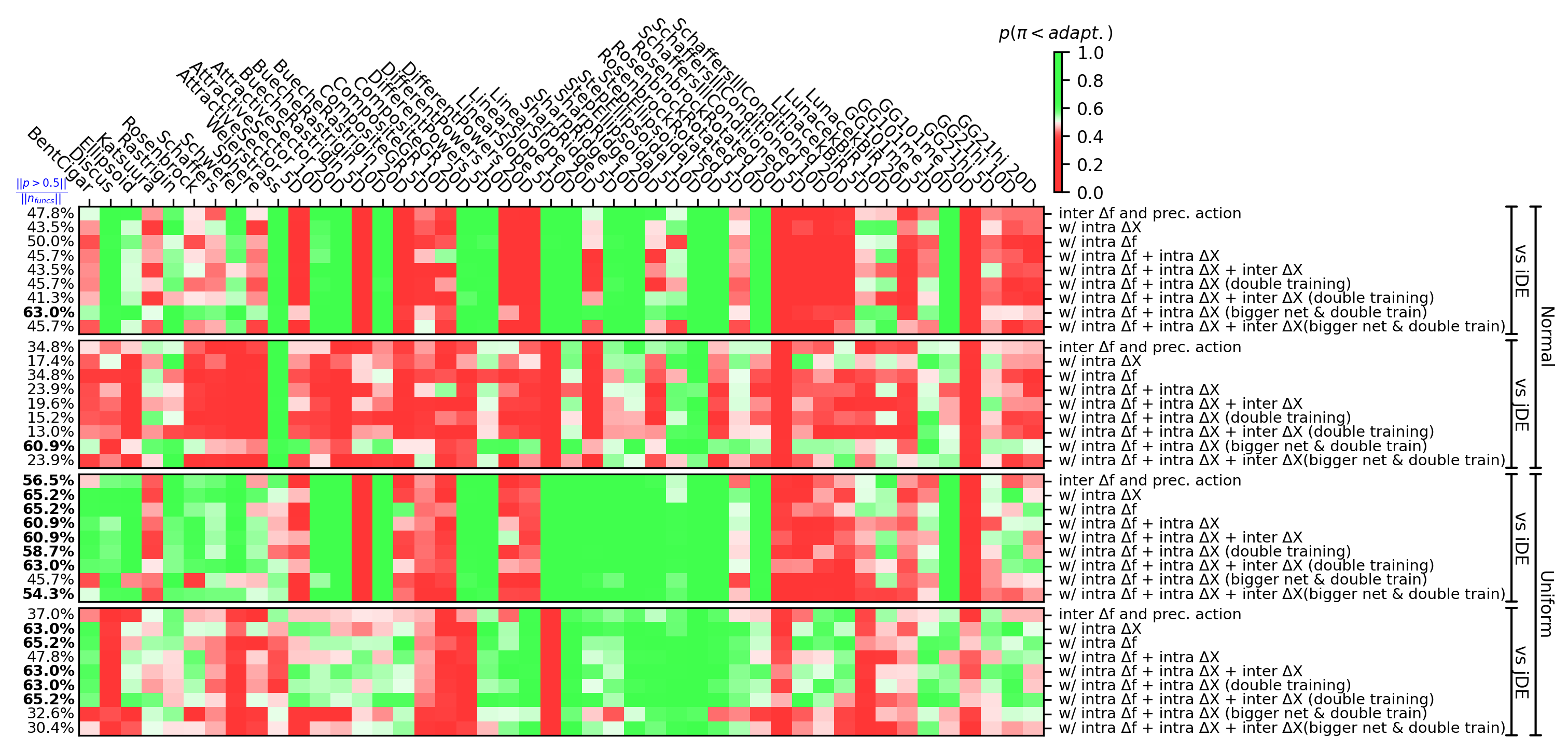
Figure 2. Multi-function training policies with different observation spaces and training times, compared with iDE (first and third row) and jDE (second and fourth row). The color is based on $p(\pi<adapt.)$, see Eq. (13), calculated on the “Best of Run” metric, where $\pi$ is the policy trained on all functions and tested on each function, and “adapt.” is either iDE or jDE. In the first two rows, the normal distribution approach is used; in the last two rows, the uniform distribution approach is used. Green (red) cells indicate that the trained policy $\pi$ works better (worse) than the corresponding adaptive DE variant. Darker green (red) indicates higher (lower) probabilities. Percentages on the left side of the rows are calculated as $\frac{\text{no. green cells}}{\text{no. green cells+no. red cells}}$ on the same row.

One of the main results that can be noted from Figure 2 is the different performance between the normal and the uniform distribution approach. The latter is visibly superior with respect to the former, and it gets very close to the single-function training performance shown in Figure 1, by only adding the intra-generational $\Delta f$ to the observation space. The normal distribution approach overcomes iDE and jDE only by both adding intra-generational $\Delta f$ and intra-generational $\Delta\boldsymbol{X}$ to the observation space and increasing the model and its training time. This suggests the fact that this approach could work but it is more difficult to train. Another consideration may be that, in order to get a better balance between exploration and exploitation, $F$ and $CR$ must be highly variant, especially at the end of the evolution.

Another important observation can be made looking at Figure 3. Because the trajectories are very similar across the functions (note that there is a small standard deviation in the actions), it is clear that the policy is not able to differentiate trough different functions, but rather it learns to map actions to the number of the current generation. Figure 3 shows only the trajectories of one policy, but the same pattern is present on all the multi-function training policies. This problem is an important limitation for the policy because being able to make different choices depending on the function is crucial if we want to have true adaptation. One possible cause of this problem may be the small capacity of the model (in terms of number of layers/neurons) or the number of episodes. However, increasing both (at least to the values that we tested) did not bring any improvement. A possible solution may be to add a loss in an intermediate layer (like GoogLeNet (Szegedy et al., 2015) does) to classify the function in some manner (e.g., unimodal or multimodal). However, this would increases the computational cost.

Figure 3 also shows that the model has learned a general policy that works well for the majority of the functions and that this is in line with the common strategy of: exploration during the first phase, and exploitation during the last phase. In fact, during the evolution, $CR$, which determines the effect of the crossover, is initially small and within a small range ($CR_{max}$ and $CR_{min}$ are $<0.5$ and similar) while at the end it increases its variance ($CR_{max}=0.75$ and $CR_{min}=0.25$). Instead, $F$, which determines the effects of mutation, is initially high with low variance (both $F_{max}$ and $F_{min}$ are $\sim 1$) and at the end it has high variance between $\sim 1$ and $\sim 0.5$.

Figure 3. Action trajectories produced by the “w/ intra $\Delta f$ uniform distribution” policy (mean $\pm$ std. dev. across $46$ benchmark functions). Given a tensor of shape $(46,50,4,50)$, storing $4$ actions of the policy during $50$ generations of $50$ evolutionary runs for each of the $46$ functions, we compute first the mean across runs, then the mean and std. dev. across functions.

5. Conclusions

In this study, we have proposed a Python framework for learning parameter adaptation policies in metaheuristics. The framework, based on a state-of-the-art RL algorithm (PPO) is of general applicability and can be easily extended to handle various optimizers and parameters thereof.

In the experimentation, we have applied the proposed framework to the learning of the step-size in CMA-ES, and the scale factor and crossover rate in DE. Our experiments demonstrate the efficacy of the learned adaptation policies, especially considering the Best of Run results in the case of DE, in comparison with well-known adaptation policies taken from the literature such as iDE and jDE.

The hybridization of metaheuristics and RL, to which this paper contributes, is becoming growing field of research, and offers the potential to create genuinely adaptive numerical optimization techniques, with the possibility to perform continual learning and incorporate previous knowledge. In this regard, this work can be extended in multiple ways. The most straightforward direction would be to test alternative RL models (different from PPO). Moreover, while in this study we focused on real-valued optimization, in principle the proposed system could be extended to handle parameter adaptation also for solving combinatorial problems. Furthermore, it will be important to test the proposed framework in real-world applications, and include in the comparative analysis other state-of-the-art optimizers. Moreover, it would be interesting to investigate alternative observation spaces and reward functions. Another option would be to extend the framework to learn the choice of operators and algorithms (in an algorithm portfolio scenario), rather than their parameters.

- (1)
- Brest et al. (2006) Janez Brest, Sao Greiner, Borko Boskovic, Marjan Mernik, and Viljem Zumer. 2006. Self-adapting control parameters in differential evolution: A comparative study on numerical benchmark problems. IEEE transactions on evolutionary computation 10, 6 (2006), 646–657.
- Burke et al. (2013) Edmund K Burke, Michel Gendreau, Matthew Hyde, Graham Kendall, Gabriela Ochoa, Ender Özcan, and Rong Qu. 2013. Hyper-heuristics: A survey of the state of the art. Journal of the Operational Research Society 64, 12 (2013), 1695–1724.
- Chakhlevitch and Cowling (2008) Konstantin Chakhlevitch and Peter Cowling. 2008. Hyperheuristics: recent developments. In Adaptive and multilevel metaheuristics. Springer, Berlin, Heidelberg, 3–29.
- Chotard et al. (2012) Alexandre Chotard, Anne Auger, and Nikolaus Hansen. 2012. Cumulative step-size adaptation on linear functions. In International Conference on Parallel Problem Solving from Nature. Springer, Berlin, Heidelberg, 72–81.
- Cotta et al. (2008) Carlos Cotta, Marc Sevaux, and Kenneth Sörensen. 2008. Adaptive and multilevel metaheuristics. Vol. 136. Springer, Berlin, Heidelberg.
- Drake et al. (2020) John H Drake, Ahmed Kheiri, Ender Özcan, and Edmund K Burke. 2020. Recent advances in selection hyper-heuristics. European Journal of Operational Research 285, 2 (2020), 405–428.
- Elsayed et al. (2011) Saber M Elsayed, Ruhul A Sarker, and Daryl L Essam. 2011. Differential evolution with multiple strategies for solving CEC2011 real-world numerical optimization problems. In 2011 IEEE Congress of Evolutionary Computation (CEC). IEEE, New York, NY, USA, 1041–1048.
- Finck et al. (2010) Steffen Finck, Nikolaus Hansen, Raymond Ros, and Anne Auger. 2010. Real-parameter black-box optimization benchmarking 2009: Presentation of the noiseless functions. Technical Report. INRIA.
- Fujimoto et al. (2018) Scott Fujimoto, Herke Hoof, and David Meger. 2018. Addressing function approximation error in actor-critic methods. In International conference on machine learning. PMLR, Stockholm, Sweden, 1587–1596.
- Ghosh et al. (2022) Arka Ghosh, Swagatam Das, Asit Kr. Das, Roman Senkerik, Adam Viktorin, Ivan Zelinka, and Antonio David Masegosa. 2022. Using Spatial Neighborhoods for Parameter Adaptation: An Improved Success History based Differential Evolution. Swarm and Evolutionary Computation in press (2022), 101057. https://doi.org/10.1016/j.swevo.2022.101057
- Hansen and Ostermeier (2001) Nikolaus Hansen and Andreas Ostermeier. 2001. Completely derandomized self-adaptation in evolution strategies. Evolutionary computation 9, 2 (2001), 159–195.
- Hu et al. (2021) Zhenzhen Hu, Wenyin Gong, and Shuijia Li. 2021. Reinforcement learning-based differential evolution for parameters extraction of photovoltaic models. Energy Reports 7 (2021), 916–928.
- Iacca et al. (2015) Giovanni Iacca, Fabio Caraffini, and Ferrante Neri. 2015. Continuous Parameter Pools in Ensemble Self-Adaptive Differential Evolution. In IEEE Symposium Series on Computational Intelligence. IEEE, New York, NY, USA, 1529–1536.
- Iacca et al. (2014) Giovanni Iacca, Ferrante Neri, Fabio Caraffini, and Ponnuthurai Nagaratnam Suganthan. 2014. A differential evolution framework with ensemble of parameters and strategies and pool of local search algorithms. In European conference on the applications of evolutionary computation. Springer, Berlin, Heidelberg, 615–626.
- Julian Blank (2022) Kalyanmoy Deb Julian Blank. 2022. Parameter Tuning and Control: A Case Study on Differential Evolution With Polynomial Mutation. https://www.egr.msu.edu/~kdeb/papers/c2022001.pdf
- LACERDA (2021) Marcelo Gomes Pereira de LACERDA. 2021. Out-of-the-box parameter control for evolutionary and swarm-based algorithms with distributed reinforcement learning. Ph. D. Dissertation. Universidade Federal de Pernambuco.
- Levine and Koltun (2013) Sergey Levine and Vladlen Koltun. 2013. Guided policy search. In International conference on machine learning. PMLR, Atlanta, GA, USA, 1–9.
- Li et al. (2017) Wenwen Li, Ender Özcan, and Robert John. 2017. A learning automata-based multiobjective hyper-heuristic. IEEE Transactions on Evolutionary Computation 23, 1 (2017), 59–73.
- Li et al. (2019) Zhihui Li, Li Shi, Caitong Yue, Zhigang Shang, and Boyang Qu. 2019. Differential evolution based on reinforcement learning with fitness ranking for solving multimodal multiobjective problems. Swarm and Evolutionary Computation 49 (2019), 234–244.
- López-Ibáñez et al. (2016) Manuel López-Ibáñez, Jérémie Dubois-Lacoste, Leslie Pérez Cáceres, Mauro Birattari, and Thomas Stützle. 2016. The irace package: Iterated racing for automatic algorithm configuration. Operations Research Perspectives 3 (2016), 43–58.
- Nareyek (2003) Alexander Nareyek. 2003. Choosing search heuristics by non-stationary reinforcement learning. In Metaheuristics: Computer decision-making. Springer, Boston, MA, USA, 523–544.
- Sallam et al. (2020) Karam M Sallam, Saber M Elsayed, Ripon K Chakrabortty, and Michael J Ryan. 2020. Evolutionary framework with reinforcement learning-based mutation adaptation. IEEE Access 8 (2020), 194045–194071.
- Sánchez et al. (2020) Melissa Sánchez, Jorge M Cruz-Duarte, José carlos Ortíz-Bayliss, Hector Ceballos, Hugo Terashima-Marin, and Ivan Amaya. 2020. A systematic review of hyper-heuristics on combinatorial optimization problems. IEEE Access 8 (2020), 128068–128095.
- Schulman et al. (2017) John Schulman, Filip Wolski, Prafulla Dhariwal, Alec Radford, and Oleg Klimov. 2017. Proximal Policy Optimization Algorithms. arXiv:1707.06347.
- Shala et al. (2020) Gresa Shala, André Biedenkapp, Noor Awad, Steven Adriaensen, Marius Lindauer, and Frank Hutter. 2020. Learning step-size adaptation in CMA-ES. In International Conference on Parallel Problem Solving from Nature. Springer, Berlin, Heidelberg, 691–706.
- Sharma et al. (2019) Mudita Sharma, Alexandros Komninos, Manuel López-Ibáñez, and Dimitar Kazakov. 2019. Deep reinforcement learning based parameter control in differential evolution. In Genetic and Evolutionary Computation Conference. ACM, New York, NY, USA, 709–717.
- Storn and Price (1997) Rainer Storn and Kenneth Price. 1997. Differential evolution–a simple and efficient heuristic for global optimization over continuous spaces. Journal of global optimization 11, 4 (1997), 341–359.
- Sun et al. (2021) Jianyong Sun, Xin Liu, Thomas Bäck, and Zongben Xu. 2021. Learning adaptive differential evolution algorithm from optimization experiences by policy gradient. IEEE Transactions on Evolutionary Computation 25, 4 (2021), 666–680.
- Sutton and Barto (2018) Richard S Sutton and Andrew G Barto. 2018. Reinforcement learning: An introduction. MIT press, Cambridge, MA, USA.
- Szegedy et al. (2015) Christian Szegedy, Wei Liu, Yangqing Jia, Pierre Sermanet, Scott Reed, Dragomir Anguelov, Dumitru Erhan, Vincent Vanhoucke, and Andrew Rabinovich. 2015. Going deeper with convolutions. In Conference on Computer Vision and Pattern recognition. IEEE, New York, NY, USA, 1–9.
- Tanabe and Fukunaga (2013) Ryoji Tanabe and Alex Fukunaga. 2013. Success-history based parameter adaptation for differential evolution. In Congress on Evolutionary Computation. IEEE, New York, NY, USA, 71–78.
- Wolpert and Macready (1997) David H Wolpert and William G Macready. 1997. No free lunch theorems for optimization. IEEE transactions on evolutionary computation 1, 1 (1997), 67–82.
- Yaman et al. (2019) Anil Yaman, Giovanni Iacca, and Fabio Caraffini. 2019. A comparison of three differential evolution strategies in terms of early convergence with different population sizes. In AIP conference proceedings, Vol. 2070. AIP Publishing LLC, Melville, NY, USA, 020002.
- Yaman et al. (2018) Anil Yaman, Giovanni Iacca, Matt Coler, George Fletcher, and Mykola Pechenizkiy. 2018. Multi-strategy differential evolution. In International Conference on the applications of evolutionary computation. Springer, Berlin, Heidelberg, 617–633.