Guided sequential ABC schemes for intractable Bayesian models

Abstract

Sequential algorithms such as sequential importance sampling (SIS) and sequential Monte Carlo (SMC) have proven fundamental in Bayesian inference for models not admitting a readily available likelihood function. For approximate Bayesian computation (ABC), SMC-ABC is the state-of-art sampler. However, since the ABC paradigm is intrinsically wasteful, sequential ABC schemes can benefit from well-targeted proposal samplers that efficiently avoid improbable parameter regions. We contribute to the ABC modeller’s toolbox with novel proposal samplers that are conditional to summary statistics of the data. In a sense, the proposed parameters are “guided” to rapidly reach regions of the posterior surface that are compatible with the observed data. This speeds up the convergence of these sequential samplers, thus reducing the computational effort, while preserving the accuracy in the inference. We provide a variety of guided Gaussian and copula-based samplers for both SIS-ABC and SMC-ABC easing inference for challenging case-studies, including multimodal posteriors, highly correlated posteriors, hierarchical models with high-dimensional summary statistics (180 summaries used to infer 21 parameters) and a simulation study of cell movements (using more than 400 summaries).

Keywords: Approximate Bayesian computation; copulas; sequential importance sampling; sequential Monte Carlo; simulation-based inference

1 Introduction

Approximate Bayesian computation (ABC) is arguably the most popular family of Bayesian samplers for statistical models characterized by intractable likelihood functions (Sisson et al., 2018). By this, we refer to many scenarios where the likelihood $p(y|\theta)$, for a dataset $y\in\mathcal{Y}$ and parameter $\theta$, is not available in closed-form or may be too cumbersome to evaluate computationally or even approximate. However, it is assumed that is feasible to simulate from the data-generating model to produce a simulated/synthetic dataset $z\sim p(z|\theta)$. The latter notation means that $z\in\mathcal{Y}$ has been implicitly generated by the likelihood function, that is, $p(z|\theta)$ is unavailable in closed form, but we can obtain simulated data $z$ from it. When the time to generate many simulated dataset is not prohibitive, ABC samplers exploit the information brought by many simulated dataset at different values of $\theta$ to learn an approximation of the posterior distribution. This is attained by comparing the several synthetic dataset $z$ with the observed $y$, possibly by first reducing the data-dimension via informative summary statistics, and rejecting the values of $\theta$ yielding simulated data that are too different from the observations. The most basic ABC sampler is the so-called ABC-rejection sampler. This typically compares features of the simulated and observed data by introducing summary statistics $S$ which reduce the dimension of $z$ as well as $y$ via $s:=S(z)$ and $s_{y}:=S(y)$, respectively (Pritchard et al., 1999). Ultimately, $s$ is compared to $s_{y}$, rather than comparing $z$ and $y$ directly, via a distance $||s-s_{y}||$ or a kernel function $K(||s-s_{y}||)$, see, e.g. Sisson et al., 2018. As an example, the ABC-rejection sampler works as follows: (i) a candidate parameter $\theta^{*}$ is proposed from the prior $\pi(\theta)$; (ii) corresponding simulated data are obtained as $z\sim p(z|\theta^{*})$, and summaries $s^{*}=S(z^{*})$ are obtained; (iii) accept and store $\theta^{*}$ if $||s^{*}-s_{y}||<\delta$ for some $\delta>0$, otherwise discard it. Steps (i)-(iii) are iterated until $N$ accepted parameters are obtained. For the reader’s benefit, a more general version of this algorithm is given in Supplementary Material K. Accepted draws from ABC-rejection are then samples from the marginal posterior

$$\pi_{\delta}(\theta|s_{y})\propto\int\mathbb{I}_{||s-s_{y}||<\delta}\cdot p(s|\theta)\pi(\theta)\mathrm{d}s$$

(with $\mathbb{I}_{A}$ being the indicator function returning 1 if $A$ is true and 0 otherwise). The ABC-rejection sampler is particularly wasteful, as the prior is used as the parameter proposal. A number of improvements to this basic algorithm has been produced in the past 20 years and are considered in Sisson et al. (2018). The most important alternative samplers are Markov chain Monte Carlo (MCMC) ABC (Marjoram et al., 2003; Sisson and Fan, 2011; Picchini, 2014) and sequential Monte Carlo ABC (SMC-ABC, Sisson et al., 2007, Beaumont et al., 2009, Del Moral et al., 2012). SMC-ABC is especially popular due to its somehow simpler tuning compared to MCMC-ABC. For example, SMC-ABC is the chosen algorithm in recent inference platforms such as ABCpy (Dutta et al., 2017) and pyABC (Schälte et al., 2022). However, ABC algorithms are generally computationally wasteful, making their use computationally challenging when simulating complex systems or inferring high-dimensional parameters. The goal of this work is to construct novel proposal functions for sequential ABC samplers (SMC-ABC and sequential importance sampling ABC), having the unique feature of being rapidly “guided” to target the region of the parameter space that is compatible with the observed data, hence considerably reducing the computational effort compared to non-guided proposals, especially in the initial iterations. We achieve this by constructing several proposal functions generating parameters conditionally to summaries of the data $s_{y}$. In particular, we construct Gaussian and copula-based proposal functions, which we call “guided proposals” due to the explicit conditioning on $s_{y}$, and show how our methods notably increase the acceptance rate of proposed parameters while thoroughly exploring the posterior surface.
Previous work exploiting information from data summaries $s_{y}$ to adjust the output of an ABC procedure is, e.g., Beaumont et al. (2002), Blum and François (2010) and Li et al. (2017). However, these approaches do not use $s_{y}$ to improve the proposal sampler during a run of some ABC algorithm, but only adjust the final output, thus acting on the already accepted parameters. Instead, our approaches make use of $s_{y}$ to guide the parameter proposals while ABC is still running. A first work in this direction is that of Bonassi and West (2015), where a joint product kernel for $(\theta,s_{y})$ is considered to derive SMC-ABC with adaptive weights, with particles sampled from a proposal (kernel) based on $\theta$ and weights based on the kernel on $s_{y}$. While computationally convenient, this independence assumption does not reflect the intrinsic dependency between $\theta$ and $s_{y}$, which we instead consider when constructing samplers for $\theta|s_{y}$. A more recent work in this direction is that of Chen and Gutmann (2019), where “regression adjustement” (Beaumont et al., 2002, Blum and François, 2010) is performed by employing neural networks. In particular, starting from many pairs $(\theta^{(i)},s^{(i)})$ simulated from the prior-predictive distribution, they regression-adjust the accepted parameters as $\theta^{(i)^{\prime}}=g(s_{y})+\theta^{(i)}-g(s^{(i)})$, where $g(\cdot)$ is a function learned by training a neural-network via early-stopping on the prior-predictive simulations. Then, they use a “best subset” of the adjusted parameters to construct a multivariate Gaussian sampler with mean $g(s_{y})$ and an inflated covariance matrix based on the $\theta^{(i)^{\prime}}$ to further propose parameters, which are then fitted using a Gaussian copula and appropriately transformed, to produce an approximated posterior as final output of the procedure.
While we also propose, among others, copula-based samplers and use the information of $s_{y}$ while ABC is running, there are several substantial differences with the approach proposed by Chen and Gutmann (2019). First, we do not need to construct a neural network architecture, hence we do not have to choose its design and the optimization schemes required for its tuning. Our approach make use of the accepted draws to construct an effective proposal sampler, without regression adjustments, as the latter are known to be effective only if the distribution of the residuals from the regression is roughly constant. Second, for some of our novel guided proposals, we introduce the ability to exploit a-priori knowledge about correlations in blocks of parameters by proposing from, say, $g(\theta_{1},\theta_{2}|s_{y},\theta_{3}^{*},\theta_{4}^{*})$ if $\theta=(\theta_{1},...,\theta_{4})$ with $(\theta_{1},\theta_{2})$ known to be highly correlated and $(\theta_{3}^{*},\theta_{4}^{*})$ being the third and fourth component of a previously accepted $\theta^{*}=(\theta_{1}^{*},...,\theta_{4}^{*})$. We have shown that this considerably ease exploration of highly correlated posteriors. Third, we do not only consider Gaussian-copulas but also Student’s t-copulas, exploring the performance of a variety of possible suggested (instead of learned via kernel density estimation) marginals such as Gaussian, location-sclae Student’s t, Gumbel, logistic, uniform and triangular, recommending the last two among all. Interestingly, the copula-based samplers are not derived starting from $(\theta,s_{y})$ (as it happens for the guided Gaussian samplers), but directly constructed for $\theta|s_{y}$. This makes them more general and flexible than the guided Gaussian proposals, derived assuming that the summary statistics are Gaussian distributed, something which may not always be true (despite this having a limited impact on the inference results, as shown here). Fourth, besides constructing guided proposals for SMC-ABC, most of our guided proposals are actually for sequential importance sampling ABC (SIS-ABC), and their performance is competitive, remarkably outperforming the state of art SMC-ABC. Ultimately, we show that our guided proposals can dramatically accelerate convergence to the bulk of the posterior by increasing acceptance rates while preserving accuracy in the posterior inference. Moreover, our methods seem to offer a viable route for inference when the dimension of the summary statistics is large, whereas SMC-ABC without guided proposals may struggle.
Other contributions for sequential likelihood-free Bayesian inference that are not within the “standard ABC” framework (i.e. procedures that are not necessarily based on specifying summary statistics that get compared via a threshold parameter $\delta$) are, e.g., Papamakarios and Murray (2016), Lueckmann et al. (2017), Papamakarios et al. (2019), Greenberg et al. (2019), Wiqvist et al. (2021), with ensemble Kalman inversion (EKI) (Chada, 2022; Duffield and Singh, 2022) being a further possibility. While these works have notable merits, we do not consider them here, as our goal is to improve the SIS-ABC and SMC-ABC samplers. However, our guided proposals may be incorporated into other samplers, e.g. EKI. In Section 2, we briefly summarize sequential ABC samplers before introducing our original proposal functions in Section 3. Simulation studies are reported in Section 4, where we consider examples with multimodal posteriors (Section 4.1), highly non-Gaussian summary statistics (Sections 4.1 and 4.4), highly correlated posteriors (section 4.2), high-dimensional parameters (Section 4.3) and high-dimensional summaries with up to 400 components (Sections 4.3 and 4.5). Finally, additional theoretical considerations, further results from the examples and setups for the simulation studies are provided as Supplementary Material. Supporting MATLAB code is available at https://github.com/umbertopicchini/guidedABC.

2 Sequential ABC schemes

Throughout this section, we summarize the key features of two of the most important sequential ABC algorithms, i.e. SIS-ABC and SMC-ABC, since they are at the core of our novel contributions.

2.1 Sequential importance sampling ABC

An obvious improvement to the basic ABC-rejection considers proposing parameters from a carefully constructed “importance sampler” $g(\theta)$. In this procedure, each accepted parameter receives a weight $\pi(\theta)/g(\theta)$ to correct for the fact that the parameter was not proposed from $\pi(\theta)$, and the weight correction provides (weighted) samples from the corresponding approximate posterior $\pi_{\delta}(\theta|s_{y})$. When $g(\theta)\equiv\pi(\theta)$, importance sampling ABC reduces to the ABC-rejection algorithm. Importance sampling is particularly appealing when embedded into a series of $T$ iterations, see Algorithm 1, which can also suggest ways to employ a decreasing sequence of thresholds $\delta_{1}<\delta_{2}<\cdots<\delta_{T}$ (more on this later). This implies the introduction of $T$ importance distributions $g_{1},...,g_{T}$, with $g_{1}(\theta)\equiv\pi(\theta)$. The output of the algorithm provides us with weighted samples from the last iteration: $(\theta^{(1)}_{T},\tilde{w}^{(1)}_{T}),\ldots,(\theta^{(N)}_{T},\tilde{w}^{(N)}_{T})$, where $\theta^{(i)}_{T}\sim\pi_{\delta_{T}}(\theta|s_{y})$. These can be used to compute the ABC posterior mean as $E(\theta|s)\approx\sum_{i=1}^{N}w^{(i)}_{T}\theta^{(i)}_{T}$ (where the $w_{t}$ denote normalized weights, i.e. $w^{(i)}_{t}=\tilde{w}^{(i)}_{t}/\sum_{j=1}^{N}\tilde{w}^{(j)}_{t}$) and posterior quantiles by using eq. (3.6) in Chen and Shao (1999). Otherwise, perhaps more practically, it is possible to sample $N$ times with replacement from the set $(\theta^{(1)}_{T},\ldots,\theta^{(N)}_{T})$, using probabilities given by the normalized weights, and then produce histograms, or compute posterior means and quantiles by using the resampled particles (after resampling, all samples have the same normalized weight $1/N$). However, Algorithm 1 does not clarify the most important issue: how to sequentially construct the samplers $g_{1},...,g_{T}$. Inspired by work on sequential learning (Cappé et al., 2004, Del Moral et al., 2006), a number of sequential ABC samplers have been produced, such as Sisson et al. (2007), Toni et al. (2008), Beaumont et al. (2009), Del Moral et al. (2012). We collectively refer to these methods as SMC-ABC, as described in Section 2.2.

Algorithm 1 Sequential importance sampling ABC (SIS-ABC)

1:Set $t:=1$.

2:for $i=1,\ldots,N$ do

3:    repeat

4:       Sample $\theta^{*}\sim\pi(\theta)$.

5:       Generate $z^{i}\sim p(z|\theta^{*})$ from the model.

6:       Compute summary statistic $s^{i}=S(z^{i})$.

7:    until $||s^{i}-s_{y}||<\delta_{1}$

8:    Set $\theta^{(i)}_{1}:=\theta^{*}$

9:    set $\tilde{w}^{(i)}_{1}:=1$.

10:end for

11:Obtain $\delta_{2}$.

12:for $t=2,\ldots,T$ do

13:    for $i=1,\ldots,N$ do

14:       repeat

15:          Sample $\theta^{*}\sim g_{t}(\theta)$.

16:          if $\pi(\theta^{*})=0$ go to step 15, otherwise continue.

17:          Generate $z^{i}\sim p(z|\theta^{*})$ from the model.

18:          Compute summary statistic $s^{i}=S(z^{i})$.

19:       until $||s^{i}-s_{y}||<\delta_{t}$

20:       Set $\theta^{(i)}_{t}:=\theta^{*}$

21:       set $\tilde{w}^{(i)}_{t}=\pi(\theta^{(i)})/g_{t}(\theta^{(i)})$.

22:    end for

23:    Decrease the current $\delta_{t}$.

24:end for

25:Output:

26:A set of weighted parameters $(\theta^{(1)}_{T},\tilde{w}^{(1)}_{T}),\ldots,(\theta^{(N)}_{T},\tilde{w}^{(N)}_{T})\sim\pi_{\delta_{T}}(\theta|s_{y})$.

2.2 Sequential Monte Carlo ABC samplers

At iteration $t$, SMC-ABC constructs automatically tuned proposal samplers by either considering “global” features of the collection of $N$ accepted samples from the previous iteration $(\theta^{(1)}_{t-1},\tilde{w}^{(1)}_{t-1}),\ldots,$ $(\theta^{(N)}_{t-1},\tilde{w}^{(N)}_{t-1})$, or “local” features that are specific to each sample $(\theta_{t-1}^{(i)},\tilde{w}_{t-1}^{(i)})$. In this framework, a sample is traditionally named “particle”. For example, a global feature could be the (weighted) sample covariance $\Sigma_{t-1}$ of the particles $(\theta^{(1)}_{t-1},...,\theta^{(N)}_{t-1})$, and this could be used in a sampler to propose particles at iteration $t$. More generally, if we consider the importance sampler as $g_{t}(\theta)\equiv g_{t}(\theta|\theta_{t-1}^{(1)},...,\theta_{t-1}^{(N)})$, we can set $g_{t}(\theta)=q(\theta|\mu_{t-1},\Sigma_{t-1})$, where $\Sigma_{t-1}$ is the previously defined covariance matrix and $\mu_{t-1}$ is some central location of the particles at iteration $t-1$. A reasonable and intuitive choice is (with some abuse of notation) $g_{t}(\theta)=q(\theta|\mu_{t-1},\Sigma_{t-1})\equiv\mathcal{N}(\mu_{t-1},\Sigma_{t-1})$, where $\mathcal{N}(a,b)$ is the $N$-dimensional Gaussian distribution with mean $a$ and covariance matrix $b$. However, this would create a global sampler that may only be appropriate if the targeted posterior is approximately Gaussian.
In SMC-ABC, the game-changer idea is the random sampling of a particle (with replacement) from the $N$ particles with associated normalized weights $(\theta^{(1)}_{t-1},{w}^{(1)}_{t-1}),\ldots$, $(\theta^{(N)}_{t-1},{w}^{(N)}_{t-1})$: call the sampled particle $\theta^{*}_{t-1}$, and then randomly “perturb” it to produce a $\theta^{**}_{t}\sim q_{t}(\cdot|\theta^{*}_{t-1})$ (notice the latter notation does not exclude dependence on other particles as well). The perturbed proposal $\theta^{**}_{t}$ may be accepted or not according to the usual ABC criterion. The procedure is iterated until $N$ proposals are accepted at each iteration. The SMC-ABC algorithm is exemplified in Algorithm 2, where the key step of sampling a particle based on its weight is in step 15, and its perturbed version is in step 16.

Algorithm 2 Sequential Monte Carlo ABC (SMC-ABC)

1:Set $t:=1$.

2:for $i=1,\ldots,N$ do

3:    repeat

4:       Sample $\theta^{*}\sim\pi(\theta)$.

5:       Generate $z^{i}\sim p(z|\theta^{*})$ from the model.

6:       Compute summary statistic $s^{i}=S(z^{i})$.

7:    until $||s^{i}-s_{y}||<\delta_{1}$

8:    Set $\theta^{(i)}_{1}:=\theta^{*}$

9:    set $\tilde{w}^{(i)}_{1}:=1$.

10:end for

11:Obtain $\delta_{2}$.

12:for $t=2,\ldots,T$ do

13:    for $i=1,\ldots,N$ do

14:       repeat

15:          Randomly pick (with replacement) $\theta^{*}$ from the weighted set $\{\theta^{(i)}_{t-1},w^{(i)}_{t-1}\}_{i=1}^{N}$.

16:          Perturb $\theta^{**}\sim q_{t}(\cdot|\theta^{*})$.

17:          if $\pi(\theta^{**})=0$ go to step 15, otherwise continue.

18:          Generate $z^{i}\sim p(z|\theta^{**})$ from the model.

19:          Compute summary statistic $s^{i}=S(z^{i})$.

20:       until $||s^{i}-s_{y}||<\delta_{t}$

21:       Set $\theta^{(i)}_{t}:=\theta^{**}$

22:       set $\tilde{w}^{(i)}_{t}=\pi(\theta^{(i)}_{t})/\sum_{j=1}^{N}{w}_{t-1}^{(j)}q_{t}(\theta^{(i)}_{t}|\theta^{(j)}_{t-1})$.

23:    end for

24:    normalize the weights: $w^{(i)}_{t}:=\tilde{w}^{(i)}_{t}/\sum_{j=1}^{N}\tilde{w}^{(j)}_{t}$.

25:    Decrease the current $\delta_{t}$.

26:end for

27:Output:

28:A set of weighted parameters $(\theta^{(1)}_{T},\tilde{w}^{(1)}_{T}),\ldots,(\theta^{(N)}_{T},\tilde{w}^{(N)}_{T})\sim\pi_{\delta_{T}}(\theta|s_{y})$.

In summary, an accepted particle $\theta^{(i)}_{t}$ results out of: (i) a randomly drawn particle from the set at iteration $t-1$ using probabilities (normalized weights) $\{w_{t-1}^{(i)}\}_{i=1}^{N}$; (ii) an additional perturbation of the particle sampled in (i). Which means that the proposal distribution for the particle $\theta^{(i)}$ is an $N$-components mixture distribution with mixing probabilities $\{w_{t-1}^{(j)}\}_{j=1}^{N}$ and components $q_{t}(\theta^{(i)}|\theta_{t-1}^{(j)})$ ($j=1,...,N$), that is
$g_{t}(\theta^{(i)})=\sum_{j=1}^{N}{w}_{t-1}^{(j)}q_{t}(\theta^{(i)}_{t}|\theta^{(j)}_{t-1})$, which motivates the importance weight

$$\tilde{w}^{(i)}_{t}=\pi(\theta^{(i)}_{t})/\sum_{j=1}^{N}{w}_{t-1}^{(j)}q_{t}(\theta^{(i)}_{t}|\theta^{(j)}_{t-1}),\qquad i=1,...,N.\vspace{-.2cm}$$ (1)

Notice that, in (1), the denominator has to be evaluated anew for each accepted $\theta^{(i)}$. One of the measures of the effectiveness of an importance or an SMC sampler is the “effective sample size” (ESS), where $1\leq\mathrm{ESS}\leq N$, the larger the ESS the better. At iteration $t$, this is traditionally approximated as $\mathrm{\widehat{ESS}}_{t}=1/\left(\sum_{j=1}^{N}(w_{t}^{(j)})^{2}\right)$, however alternatives are explored in Martino et al. (2017).
Some notable SMC-ABC proposal samplers for $\theta_{t}^{**}\sim q_{t}(\cdot|\theta_{t-1}^{*})$ are detailed in the Supplementary Material K. Here, we briefly recall the two samplers that provide a useful comparison with our novel methods introduced in Sections 3. Some of the most interesting work for the construction of such samplers is in Filippi et al. (2013), where particles randomly picked from the previous iterations are perturbed with Gaussian proposals with several proposed tuning of the covariance matrix, improving on Beaumont et al. (2009). As a first approach, Filippi et al. (2013) propose the full $\theta^{**}$ by generating at iteration $t$ from the $d_{\theta}$-dimensional Gaussian $q(\theta|\theta^{*})\equiv\mathcal{N}(\theta^{*},2\Sigma)$, with $\Sigma$ being the empirical weighted covariance matrix from the particles accepted at iteration $t-1$. This results in the importance weights (1) becoming (with the usual notation abuse) $\tilde{w}^{(i)}_{t}=\pi(\theta^{(i)}_{t})/\sum_{j=1}^{N}{w}_{t-1}^{(j)}\mathcal{N}(\theta^{(i)}_{t};\theta^{(j)}_{t-1},2\Sigma_{t-1})$, where $\mathcal{N}(x;a,b)$ denotes the probability density function of a Gaussian distribution with mean $a$ and covariance matrix $b$ evaluated at $x$. In our experiments, this proposal embedded into SMC-ABC is denoted standard, being in some way a baseline approach. Having $\theta^{**}_{t}\sim\mathcal{N}(\theta^{*}_{t-1},2\Sigma_{t-1})$ implies that the mean of the proposal sampler exploits “local” features, since perturbed draws lie within an ellipsis centred in $\theta^{*}_{t}$, while its covariance matrix is still global. To obtain a “local” covariance, Filippi et al. (2013) proposed the “optimal local covariance matrix” (olcm) sampler. The key feature of this sampler is that each proposed particle $\theta^{**}$ arises from perturbing $\theta^{*}$ using a Gaussian distribution having a covariance matrix that is specific to $\theta^{*}$ (hence “local”), rather than being tuned on all particles accepted at $t-1$ as in the standard sampler. To construct the olcm, Filippi et al. (2013) define the following weighted set of particles of size $N_{0}\leq N$ at iteration $t-1$

$$\{\tilde{\theta}_{t-1,l},\gamma_{t-1,l}\}_{1\leq l\leq N_{0}}=\biggl{\{}\biggl{(}{\theta}_{t-1}^{(i)},\frac{w_{t-1}^{(i)}}{\bar{\gamma}_{t-1}}\biggr{)},\text{ s.t. }||s^{i}_{t-1}-s_{y}||<\delta_{t},\quad i=1,...,N\biggr{\}},$$ (2)

where $\bar{\gamma}_{t-1}$ is a normalisation constant such that $\sum_{l=1}^{N_{0}}\gamma_{t-1,l}=1$. That is, the $N_{0}$ weighted particles are the subset of the $N$ particles accepted at iteration $t-1$ (when using $\delta_{t-1}$) having generated summaries that produce distances that are also smaller than $\delta_{t}$. We used the letter $\gamma$ to denote normalized weights associated to the subset of $N_{0}$ particles, rather than $w$, to avoid confusion. At iteration $t$, the olcm proposal is $q_{t}(\theta|\theta^{*})=\mathcal{N}(\theta^{*},\Sigma^{\mathrm{olcm}}_{\theta^{*}})$, where $\Sigma^{\mathrm{olcm}}_{\theta^{*}}=\sum_{l=1}^{N_{0}}\gamma_{t-1,l}(\tilde{\theta}_{t-1,l}-\theta^{*})(\tilde{\theta}_{t-1,l}-\theta^{*})^{\prime}$, where ^′ denotes transposition throughout our work. Accepted particles are then given unnormalized weights $\tilde{w}^{(i)}_{t}=\pi(\theta^{(i)}_{t})/\sum_{j=1}^{N}{w}_{t-1}^{(j)}\mathcal{N}(\theta^{(i)}_{t};\theta^{(j)}_{t-1},\Sigma^{\mathrm{olcm}}_{\theta^{(j)}})$. Note that we are required to store the $N$ distances $||s^{i}_{t-1}-s_{y}||$ accepted at iteration $t-1$ to be able to determine which indices $i$ have distance smaller than the $t$-th threshold $\delta_{t}$, i.e. $||s^{i}_{t-1}-s_{y}||<\delta_{t}$. Evaluating $\Sigma^{\mathrm{olcm}}_{\theta^{*}}$ causes some non-negligible overhead in the computations, since it has to be performed for every proposal parameter, and therefore sanity checks are required at every proposal to ensure that it results in a positive definite covariance matrix, or otherwise computer implementations will halt with an error. We postpone such discussion in Section 3.5, where it is better placed, and introduce now our novel proposal samplers.

3 Guided sequential samplers

Here, we describe our main contributions to improve the efficiency of both SIS-ABC and SMC-ABC samplers by constructing proposals that are conditional on observed summaries $s_{y}$, to guide the particles by using information provided by the data. In particular, we create proposal samplers of type $g(\theta|s_{y})$ (when the entire vector parameter is proposed in block) or even conditional proposals of type $g(\theta_{k}|\theta_{-k},s_{y})$, where $\theta_{k}$ is the $k$-th component of a $d_{\theta}$-dimensional vector parameter $\theta$ and $\theta_{-k}=(\theta_{1},...,\theta_{k-1},\theta_{k+1},...,\theta_{d_{\theta}})$. The starting idea behind the construction of these samplers is loosely inspired by Picchini et al. (2022), where a guided Gaussian proposal is constructed for MCMC inference using synthetic likelihoods (Wood, 2010; Price et al., 2018). This initial inspiration is significantly expanded in multiple directions, e.g. by providing strategies to avoid the “mode-seeking” behaviour of the basic guided proposals, by constructing the above mentioned proposals of type $g(\theta_{k}|\theta_{-k},s_{y})$ and by introducing non-Gaussian proposal samplers using copulas with a variety of marginal structures, yielding an ABC methodology capable to tackle considerably challenging problems. To help the reader navigate through the several proposals samplers introduced in this work, we classify them in Table 1.

Proposal sampler	Guided	Family	Global or local	Algorithm	Section
standard	no	Gaussian	local mean, global cov	SMC-ABC	2.2
olcm	no	Gaussian	local mean, local cov	SMC-ABC	2.2
blocked	yes	Gaussian	global mean, global cov	SIS-ABC	3.1
blockedopt	yes	Gaussian	global mean, global cov	SIS-ABC	3.2
hybrid	yes	Gaussian	global mean, global cov	SIS-ABC	3.3
cop-blocked	yes	Gaussian or t copula	global mean, global cov	SIS-ABC	3.4
cop-blockedopt	yes	Gaussian or t copula	global mean, global cov	SIS-ABC	3.4
cop-hybrid	yes	Gaussian or t copula	global mean, global cov	SIS-ABC	3.4
fullcond	yes	Gaussian	local mean, global var	SMC-ABC	3.5
fullcondopt	yes	Gaussian	local mean, local var	SMC-ABC	3.6

Table 1: Proposal samplers considered in this work, categorized according to whether the sampler is guided by data or not, its distributional family, whether the sampler has features that are specific for each particle (local) or common to all particles (global), the type of algorithm employing the proposal sampler and the relevant section introducing it. All listed samplers are novel, except for standard and olcm.

In Section 3.1, we consider a first approach for a guided Gaussian proposal function for SIS-ABC, whose covariance matrix is in some sense optimized in Section 3.2. A hybrid approach combining the two is proposed in Section 3.3. Then, Section 3.4 generalizes the guided Gaussian approaches for SIS-ABC to copula-based proposals, constructing a sampler directly for $\theta|s_{y}$ instead of deriving it starting from a Gaussian sampler $g(\theta,s_{y})$. Finally, in Section 3.5, we propose a guided Gaussian SMC-ABC scheme, whose covariance matrix is then optimized in Section 3.6.

3.1 A first guided Gaussian SIS-ABC sampler

In Picchini et al. (2022), an MCMC proposal sampler was constructed to aid inference via synthetic likelihoods (Wood, 2010, Price et al., 2018). There, the idea was to collect the several (say $L$) model-simulated summary statistics $\{s^{i}\}_{i=1}^{L}$ that were generated at a given proposed parameter $\theta$, average them to obtain ${\color[rgb]{0,0,0}\bar{s}=\sum_{i=1}^{L}s^{i}/L}$ so that, by appealing to the Central Limit Theorem, for $L$ “large” enough, $\bar{s}$ was approximately Gaussian distributed. Picchini et al. (2022) then observed that if the joint $(\theta,\bar{s}^{i})$ is approximately multivariate Gaussian, then a conditionally Gaussian $g(\theta|s=s_{y})$ can be constructed and used as a proposal sampler.
Let us now set $d_{\theta}=\dim(\theta),d_{s}=\dim(s_{y}),d=d_{\theta}+d_{s}$ and denote by $(\theta^{(i)},s^{(i)})$ a $d$-dimensional particle that has been accepted at iteration $t-1$ of SIS-ABC. Assume for a moment that $(\theta^{(i)},{s}^{(i)})$ is a $d$-dimensional Gaussian distributed vector $(\theta^{(i)},{s}^{(i)})\sim\mathcal{N}_{d}(m,S)$. We stress that this assumption is made merely to construct a proposal sampler, and does not extend to the actual distribution of $(\theta^{(i)},s^{(i)})$. We set a $d$-dimensional mean vector $m\equiv(m_{\theta},m_{s})$ and the $d\times d$ covariance matrix

$${S}\equiv\left[\begin{array}[]{cc}{S}_{\theta}&{S}_{\theta s}\\ {S}_{s\theta}&{S}_{s}\\ \end{array}\right],$$

where ${S}_{\theta}$ is $d_{\theta}\times d_{\theta}$, ${S}_{s}$ is $d_{s}\times d_{s}$, ${S}_{\theta s}$ is $d_{\theta}\times d_{s}$ and of course ${S}_{s\theta}\equiv{S}_{\theta s}^{\prime}$ is $d_{s}\times d_{\theta}$. Once all $N$ accepted particles have been collected for iteration $t-1$ of the SIS-ABC sampler, we estimate $m$ and $S$ using the accepted (weighted) particles. That is, denote by $x^{(i)}_{t-1}:=(\theta^{(i)}_{t-1},{s}^{(i)}_{t-1})$ a $d$-dimensional particle accepted at iteration $t-1$. By using their normalized weights, we have the following estimated weighted mean and weighted covariance matrix

$$\hat{m}_{t-1}=\sum_{i=1}^{N}{w^{(i)}_{t-1}}x^{(i)}_{t-1},\qquad\hat{S}_{t-1}=\frac{1}{(1-\sum_{i=1}^{N}{w_{t-1}^{(i)}}^{2})}\sum_{i=1}^{N}w^{(i)}_{t-1}(x_{t-1}^{(i)}-\hat{m}_{t-1})(x^{(i)}-\hat{m}_{t-1})^{\prime}$$ (3)

(snippets of vectorized code to efficiently compute (3) are reported in the Supplementary Material D). Once $\hat{m}_{t-1}$ and $\hat{S}_{t-1}$ are obtained, it is possible to extract the corresponding entries $\hat{m}_{\theta}$, $\hat{m}_{s}$ and $\hat{S}_{\theta}$, $\hat{S}_{s}$, $\hat{S}_{s\theta}$, $\hat{S}_{\theta s}$, where we have disregarded the “$t-1$” iteration subscript to simplify the notation. We can then use well known formulas for the conditional distributions of a multivariate Gaussian, to obtain a proposal distribution for iteration $t$ given by $g_{t}(\theta|s_{y})\equiv\mathcal{N}(\hat{m}_{\theta|s_{y},t-1},\hat{S}_{\theta|s_{y},t-1})$, with

$$\hat{m}_{\theta|s_{y},t-1} =\hat{m}_{\theta}+\hat{S}_{\theta s}(\hat{S}_{s})^{-1}(s_{y}-\hat{m}_{s})$$ (4)

$$\hat{S}_{\theta|s_{y},t-1} =\hat{S}_{\theta}-\hat{S}_{\theta s}(\hat{S}_{s})^{-1}\hat{S}_{s\theta},$$ (5)

and weights (1) given by $\tilde{w}^{(i)}_{t}=\pi(\theta_{t}^{(i)})/\mathcal{N}(\hat{m}_{\theta|s_{y},t-1},\hat{S}_{\theta|s_{y},t-1})$, $i=1,...,N$. Hence, a parameter proposal for Algorithm 1 can be generated as $\theta^{*}\sim\mathcal{N}(\hat{m}_{\theta|s_{y},t-1},\hat{S}_{\theta|s_{y},t-1})$, which has an explicit “guiding” term $(s_{y}-\hat{m}_{s})$. We call $g_{t}(\theta|s_{y})$ a “guided SIS-ABC sampler”. To distinguish it from other guided SIS-ABC samplers we introduce later, this one is named blocked, since all coordinates of $\theta^{*}$ are proposed jointly, hence “in block”.
Note that the guiding term $(s_{y}-\hat{m}_{s})$ becomes less and less relevant as $\hat{m_{s}}\approx s_{y}$, which is supposed to happen when $\delta$ is small enough. Of course, a concern around the efficacy of such sampler may arise if the joint $(\theta,s)$ is not approximately multivariate Gaussian. The case study in Sections 4.1 and 4.4 (and in Supplementary Material E and H) have markedly non-Gaussian summary statistics, but our guided sampler behaves well. However, an undesirable feature is that it may occasionally display “mode-seeking” behaviour, i.e., it may rapidly approach high posterior density areas, quickly accepting promising particles in the initial iterations, but it may ending up exploring mostly the area around the posterior mode and not necessarily the tails of the targeted distribution. We address this issue in the next section by tuning the covariance matrix of the sampler while preserving its “guided” feature.

3.2 Guided Gaussian SIS-ABC sampler with optimal local covariance

Proposal samplers can be designed according to several intuitions. For example, they could be based on the similarity with the targeted density, as suggested by a small Kullback-Leibler (KL) divergence while maximizing the acceptance probability as in Filippi et al., 2013, or based on minimizing the variance of the importance weights while maximizing the acceptance probability as in Alsing et al. (2018), or using guided approaches as those outlined before. Here, we let the mean of a Gaussian sampler to be the same as in (4), hence the proposal is guided by the observed summaries, but we construct the proposal covariance matrix following a reasoning inspired by Filippi et al. (2013) for SMC-ABC, and extended here to accommodate SIS-ABC.
For the “target” distribution denoted by $q^{*}_{\delta_{t}}(\theta^{*})=\pi_{\delta_{t}}(\theta^{*}|s_{y})$, we wish to determine a proposal $q_{\delta_{t}}(\theta^{*})$ by minimizing the KL divergence $KL(q_{\delta_{t}},q^{*}_{\delta_{t}})$ between its arguments, where

$$KL(q_{\delta_{t}},q^{*}_{\delta_{t}})=\int q^{*}_{\delta_{t}}(\theta^{*})\log\frac{q^{*}_{\delta_{t}}(\theta^{*})}{q_{\delta_{t}}(\theta^{*})}d\theta^{*}.$$

In the context of SMC-ABC, which we discuss later in Section 3.6, Filippi et al. (2013) mention that it is possible to consider a “multi-objective optimization” problem where, in addition to minimize the KL divergence, the maximization of an “average acceptance probability” is also carried out. By transposing their reasoning to our SIS-ABC context, the multi-objective optimization is equivalent to maximizing the following quantity

$$Q(q_{t},\delta_{t},s_{y})=\int\pi_{\delta_{t}}(\theta^{*}|s_{y})\log q_{t}(\theta^{*})d\theta^{*}$$ (6)

with respect to $q_{t}$. By considering $q_{t}(\theta^{*})\equiv\mathcal{N}(\hat{m}_{\theta|s_{y},t-1},\Sigma_{t})$ for unknown $\Sigma_{t}$ and fixed $\hat{m}_{\theta|s_{y},t-1}$ defined as in (4), the resulting maximization in $\Sigma_{t}$ leads to (details are in Supplementary Material A)

$$\Sigma_{t}=\int\pi_{\delta_{t}}(\theta^{*}|s_{y})(\theta^{*}-\hat{m}_{\theta|s_{y},t-1})^{\prime}(\theta^{*}-\hat{m}_{\theta|s_{y},t-1})d\theta^{*}.$$ (7)

The latter integral can be approximated following the same reasoning for olcm, detailed in the Supplementary Material A. Namely, we can consider the $N$ particles accepted at iteration $t-1$ (which used a threshold $\delta_{t-1}$) and select from those the $N_{0}\leq N$ particles that produced a distance $||s-s_{y}||$ that is also smaller than $\delta_{t}$, to obtain $\hat{\Sigma}_{t}=\sum_{l=1}^{N_{0}}\gamma_{t-1,l}(\tilde{\theta}_{t-1,l}-\hat{m}_{\theta|s_{y},t-1})(\tilde{\theta}_{t-1,l}-\hat{m}_{\theta|s_{y},t-1})^{\prime}$, with $(\tilde{\theta},\gamma)$ defined as in (2). We call blockedopt a SIS-ABC sampler with $g_{t}(\theta|s_{y})\equiv\mathcal{N}(\hat{m}_{\theta|s_{y},t-1},\hat{\Sigma}_{t})$ as guided proposal. Importantly, notice that unlike olcm, the covariance matrix $\hat{\Sigma}_{t}$ is “global”, which means that at each iteration only one covariance matrix needs to be computed and used for all proposed particles. This relieves the computational budget from the necessity to ensure (via Cholesky decomposition and in case of numerical issues, a more expensive modified-Cholesky decomposition as in Higham, 1988) that the particle-specific covariance matrix is positive definite for each proposed particle. Of course, there is appeal in having a particle-specific “local” covariance matrix, and this is explored in Section 3.5.

3.3 Hybrid guided Gaussian SIS-ABC sampler

We consider a further type of guided Gaussian SIS-ABC sampler, which we denote hybrid, which is a by-product of the blocked and blockedopt strategies. At iteration $t=1$, the hybrid sampler proposes from the prior, as in all examined strategies. At $t=2$, it proposes using blocked for rapid convergence towards the modal region, while for $t>2$, it uses blockedopt to correct for possible mode-seeking behaviour.

3.4 Guided copula-based SIS-ABC samplers

The previously proposed guided Gaussian SIS-ABC samplers assume an underlying Gaussian distribution for $(\theta,s_{y})$, which is then used to construct the proposal $g_{t}(\theta|s_{y})$, which follows a $d_{\theta}$-dimensional Gaussian distribution with a certain mean vector $m^{*}$ and covariance matrix $S^{*}=(S^{*}_{ij})_{i,j=1}^{d}$. This can be generalised by dropping the assumption of Gaussianity on $(\theta,s_{y})$, making the samplers $g_{t}(\theta|s_{y})$ more flexible, both in terms of joint distribution and marginals. To do this, we use copulas, proposing what we call cop-blocked, cop-blockedopt, cop-hybrid, the copula-based versions of blocked, blockedopt and hybrid, respectively, with a few key differences though, as discussed in Remarks 1 and 2 below. The idea of using copula modelling within ABC has been proposed e.g. by Li et al. (2017), who use a Gaussian copula for approximating the ABC posterior for a high-dimensional parameter space, and by An et al. (2020) for modelling a high-dimensional summary statistic. Instead, we use (Gaussian and t) copulas for the proposal sampler $g_{t}(\theta|s_{y})$ (and not for the kernel for $(\theta,s_{y}))$.
Suppose that the $d_{\theta}$-dimensional random vector $X=(X_{1},\ldots,X_{d_{\theta}})$ has a joint cumulative distribution function $H$ and continuous marginals $F_{1},\ldots,F_{d}$, i.e., $X\sim H(F_{1}(x_{1}),\ldots,F_{d}(x_{d_{\theta}}))$. Sklar’s theorem (Sklar, 1959) states that the joint distribution $H$ can be rewritten in terms of ${d_{\theta}}$ uniform marginal distributions and a multivariate copula function $C:[0,1]^{d_{\theta}}\to[0,1]$ that describes the correlation structure between them, i.e.

$$H(x_{1},\ldots,x_{d_{\theta}})=C(u_{1},\ldots,u_{d_{\theta}})=C(F_{1}(x_{1}),\ldots,F_{d_{\theta}}(x_{d_{\theta}})),$$

with $u_{j}=F_{j}(x_{j}),j=1,\ldots,{d_{\theta}}$. Hence, a copula is a multivariate distribution with uniform marginals. Denoting by $h$, $f_{j}$ and $c$ the densities of the joint distribution $H$, the marginal $F_{j}$ and the copula $C$, respectively, we have

$$h(x_{1},\ldots,x_{d_{\theta}})=c(u_{1},\ldots,u_{d_{\theta}})\prod_{i=1}^{d_{\theta}}f_{j}(x_{j}),\qquad j=1,\ldots,{d_{\theta}},\vspace{-.2cm}$$ (8)

where $c(u_{1},\ldots,{d_{\theta}})=\frac{\partial^{d_{\theta}}}{\partial u_{1}\cdots\partial u_{d_{\theta}}}C(U_{1},\ldots,U_{d_{\theta}}).$ As copula families $C$, we consider the Gaussian and the $t$ copulas, corresponding on having the joint distribution $H$ to be a multivariate Gaussian and a Student’s $t$, respectively. While the Gaussian copula is fully characterised by a correlation matrix $R$, the $t$ copulas depend on both a correlation matrix $R$ and the degrees of freedom $\nu$, a hyperparameter which we fix to five (see details in Supplementary Material B). Both are members of the class of elliptical copulas, which may also be considered (Embrechts et al., 2002). Other copula families (e.g. Archimedean copulas) are available, but they do not allow for negative correlations in dimensions larger than two. Vine copulas (Bedford and Cooke, 2002) may be used to tackle this, but they are not immediate to construct, limiting their use in this context. Notice that the correlation matrix of a Gaussian (and t) copula with correlation parameter $R$ is, in general, not $R$, unless all marginals are normal, in which case the Gaussian copula coincides with a multivariate normal. This is because the covariance of $(X_{i},X_{j})$ is not invariant for strictly monotone functions, and does, thus, depend on the underlying marginals $F_{i},F_{j}$, see Hoeffding (1940) and Embrechts et al. (2002). For this reason, here we consider the Kendall’s $\tau$, a rank correlation which has the properties of being invariant under monotone transformation, of depending only on the copulas (Embrechts et al., 2002) and of being easier to compute analytically than the Spearman’s rho, another dependent measure having similar properties. In particular, the Kendall’s $\tau$ of two random variables $X_{i},X_{j}$ with Gaussian or $t$ copulas with correlation parameter $R_{ij}$ is given by $\tau_{ij}:=\tau(X_{i},X_{j})=2/{\pi}\arcsin{R_{ij}}$. Hence, when choosing the copula and the underlying marginals, we want to preserve the mean vector $m^{*}$, the variances $S^{*}_{ii},i=1,\ldots,d_{\theta}$ and the Kendall’s tau dependencies of the guided Gaussian SIS-ABC samplers. To do this, we derive the Kendall’s $\tau$ dependencies from the correlation parameter $R$, derived from $S^{*}$, choosing the parameters of the underlying marginal distributions $F_{j}$ such that $\mathbb{E}[X_{j}]=m_{j}^{*}$ and $\textrm{Var}(X_{j})=S_{jj}^{*}$. Hence, a $d_{\theta}$-dimensional parameter proposal $\theta^{*}\sim g_{t}(\theta|s_{y})$ with copula $C$, marginals $F_{1},\ldots,F_{d_{\theta}}$, mean vector $m^{*}$, variances $S_{ii}^{*}$ and Kendall’s tau rank correlations $\tau_{ij},i,j=1\ldots,d_{\theta},i\neq j$ for SIS-ABC can be generated as follows:

1. Derive the parameters of the marginal distribution $F_{j}$ such that $\mathbb{E}[X_{j}]=m_{j}^{*}$ and $\textrm{Var}(X_{j})=S^{*}_{jj},j=1,\ldots,d_{\theta}$.

2. Compute the correlation matrix $R=(R_{ij})_{i,j=1}^{d}$ from the covariance matrix $S^{*}=(S^{*}_{ij})_{i,j=1}^{d}$, with entries

   $$R_{ij}=\frac{\textrm{Cov}(X_{i},X_{j})}{\sqrt{\textrm{Var}(X_{i})\textrm{Var}(X_{j})]}}=\frac{1}{\sqrt{S_{ii}^{*}S_{jj}^{*}}}S_{ij}^{*}.\vspace{-.2cm}$$

3. Simulate $(u_{1},\ldots,u_{d_{\theta}})$ from the chosen (Gaussian or t) copula with correlation $R$.

4. Set $\theta^{*}_{j}:=x_{j}=F_{j}^{-1}(u_{j})$ to obtain the desired parameter proposals with Kendall’s tau $\tau_{ij}=2/\pi\arcsin{R_{ij}},i,j=1,\ldots,d_{\theta},i\neq j$.

For step 1, calculations linking the parameters of the chosen marginal distributions to the marginal mean $m^{*}_{j}$ and variance $S^{*}_{jj}$ are reported in Supplementary Material C. Note that step 4 is well defined thanks to the marginal distributions being continuous. Finally, the proposal density needed to derive the weights of the $i$th particle (line 21 of Algorithm 1) can be computed via (8), using the copula densities reported in Supplementary Material B. As no information is available on $\theta_{j}|s_{y}$, we choose all underlying marginal distributions $F_{j}$ to be from the same family. Distinct families could be also considered, as discussed in Remark 3 below. Here, as underlying marginal distributions $F_{j}$, we choose the location-scale Student’s t (with $\nu$ degrees of freedom, see Supplementary Material C for more details), the logistic, the Gumbel, the Gaussian, the triangular and the uniform distribution. The normal distribution is chosen to favour a comparison with the corresponding guided Gaussian SIS-ABC samplers (when choosing a Gaussian copula with the right setting, see Remark 2 below). The first three marginals (resp. last two) are chosen as they have heavier (resp. lighter) tails than the Gaussian distribution, allowing to sample less (resp. more) around their mean values. Moreover, the Gumbel distribution is also chosen to evaluate the impact of (positive) skewness on the results, as all other marginals are symmetric. We refer to the Supplementary Material C for an extensive discussion and comparison of the marginals.

Remark 1.

The guided Gaussian proposal samplers $g_{t}(\theta|s_{y})$, derived in the previous sections, are constructed under the assumption of $(\theta,s_{y})$ being Gaussian, thus requiring also the distribution of the summary to be Gaussian, which may not always be true (despite having a limited impact on the estimation procedure, as shown in Section 4). Instead, the guided copula-based proposal sampler $g_{t}(\theta|s_{y})$ is directly constructed on $\theta|s_{y}$, without assumptions on the distribution of the summaries $s_{y}$ and/or of $(\theta,s_{y})$.

Remark 2.

Sampling from a Gaussian copula with normal marginals and correlation parameter $R$ corresponds to sampling from a multivariate Gaussian proposal with correlation matrix $R$ (Embrechts et al., 2002). Hence, cop-blocked, cop-blockedopt and cop-hybrid for the conditional sampler $g_{t}(\theta|s_{y})$ with this setting coincide with blocked, blockedopt and hybrid for $\theta|s_{y}$, respectively. However, even in this setting, the copula-based distribution of $(\theta,s_{y})$ would differ from $N_{d}(m,S)$, the joint Gaussian distribution used to construct the guided Gaussian proposals, unless $s_{y}\sim N_{d_{s}}(m_{s},S_{s})$.

Remark 3.

The guided copula-based SIS-ABC samplers introduce more flexibility than the guided Gaussian ones, e.g. in the choice of the copula, the marginals (which may belong to different distribution families or change across iterations, see the “mixed” marginals introduced in Section 4) and their underlying parameters (e.g. the degrees of freedom of the $t$ copula or of the location-scale Student’s t marginals). In the simulation studies considered here, the copula and marginal models are fixed in advance, with the idea of investigating whether a particular combination of copula and marginals outperforms the other consistently across the experiments. Moreover, it is worth stressing that the marginal proposals are not for $\theta_{j}$, for which some information may be available (e.g. their support) and used in the choice of the marginals, but for $\theta_{j}|s_{y}$, for which less is known (e.g., the support will differ from that of $\theta_{j}$). Hence, unless some prior knowledge is assumed/known about $\theta_{j}|s_{y}$, we recommend using marginal distributions assuming also negative values. Two alternative possibilities could be to perform a kind of “regression adjustment” within each iteration, e.g. by fitting suitable marginals and copula in the spirit of Chen and Gutmann, 2019, or run a non-parametric estimation of the copula and the marginals. However, these two approaches would introduce some extra computational costs though, which is why we do not consider them here.

3.5 Guided Gaussian SMC-ABC samplers

Here, we wish to make the proposal function $g_{t}$ more dependent on the local features of important particles from the set obtained at iteration $t-1$, as in standard SMC-ABC proposal samplers. As previously discussed, choosing $\theta^{**}\sim\mathcal{N}(\theta^{*},2\Sigma_{t-1})$ in step 16 of Algorithm 2 as in Filippi et al. (2013) yields a particle-specific mean (local feature) and a covariance matrix which is common to all particles (global feature). With reference to Gaussian samplers, we can construct samplers where each proposed particle at iteration $t$ has its own specific mean and a global covariance structure and, additionally, be conditional on observed summaries $s_{y}$.
Constructing a guided and local SMC-ABC sampler is immediate given the reasoning in Sections 3.1-3.3. Remember that we wish to perturb a sampled particle $\theta^{*}$ to produce a proposed $\theta^{**}$ in step 16 of Algorithm 2. Once $\theta^{*}$ has been sampled from the accepted particles at iteration $t-1$, we define as “augmented data” the vector $(\theta^{*},s_{y})$, which we want to use to produce $\theta^{**}$. It is useful to imagine $\theta^{*}$ as $(\theta^{*}_{k},\theta_{-k}^{*})$ if we wish to update one component at a time, using the notation established at the beginning of Section 3, or as $(\theta^{*}_{k,l},\theta_{-(k,l)}^{*})$ if we update a block of two components at a time, etc. In Section 4.2, we consider an example where some components of $\theta$ are highly correlated in the prior, and a sampler exploiting this fact dramatically helps producing an efficient ABC algorithm. We illustrate this conditional approach by focusing on perturbing a single component of $\theta$, as the notation is easier to convey the message and extensions to multiple components are immediate. Hence, here we focus on the augmented data expressed as the column vector $(\theta_{k}^{*},\theta_{-k}^{*},s_{y})^{\prime}$, for which we assume a joint multivariate Gaussian distribution allowing us to design a “perturbation kernel” $q_{t}(\theta_{k}|\theta_{-k}^{*},s_{y})$. Our goal is proposing for the $k$-th component of $\theta$ conditionally on the remaining $d_{\theta}-1$ coordinates of $\theta^{*}$ and the whole $s_{y}$. This means that the sampler producing $\theta^{**}_{k}$ does not make use of the value of $\theta_{k}^{*}$, but the sampler producing $\theta^{**}_{k^{\prime}}$ will make use of $\theta_{k}^{*}$ ($k^{\prime}\neq k$). Under the same assumptions of joint Gaussianity considered in Sections 3.1-3.3, we have that $q_{t}(\theta_{k}|\theta_{-k}^{*},s_{y})$ is a Gaussian sampler, which we now construct.
Say that all $N$ accepted $d$-dimensional particles of type $(\theta,s)$ have been obtained for iteration $t-1$. We now compute the weighted sample mean and weighed covariance matrix as in (3), and from these we extract the following quantities

• $\hat{m}_{k}$: scalar element extracted from $\hat{m}_{t-1}$ and corresponding to component $k$ of $\theta$;

• $\hat{S}_{k,-k}$: $(d-1)$-dimensional row vector extracted from $\hat{S}_{t-1}$ by considering the row corresponding to $\theta_{k}$ and retaining all columns except that corresponding to $\theta_{k}$.

• $\hat{S}_{-k,-k}$: $(d-1)\times(d-1)$-dimensional matrix extracted from $\hat{S}_{t-1}$ by eliminating the row and column corresponding to $\theta_{k}$.

• $\begin{bmatrix}\theta^{*}_{-k}\\ s_{y}\end{bmatrix}$ : $(d-1)$-dimensional column vector appending $s_{y}$ to the particle $\theta^{*}_{-k}$, where the latter is the $\theta^{*}$ randomly picked in step 15 of Algorithm 2 with its $k$-th component eliminated.

• $\begin{bmatrix}\hat{m}_{-k}\\ \hat{m}_{s}\end{bmatrix}$: $(d-1)$-dimensional column vector concatenating the $d_{\theta}-1$ (weighted) sample means of the particles for $\theta$, except the $k$-th component, and the $d_{s}$ (weighted) sample means of the corresponding summary statistics.

• $\hat{\sigma}^{2}_{k}$: scalar value found in $\hat{S}_{t-1}$ correspondingly to the row and column entry for $\theta_{k}$.

• $\hat{S}_{-k,k}$: $(d-1)$-dimensional column vector extracted from $\hat{S}_{t-1}$ by retaining all rows except that corresponding to $\theta_{k}$, and considering only the column corresponding to $\theta_{k}$.

Then, upon completion of iteration $t-1$, we have

$$\hat{m}_{k|s_{y},t-1}^{*} = \hat{m}_{k}+\hat{S}_{k,-k}(\hat{S}_{-k,-k})^{-1}\biggl{(}\begin{bmatrix}\theta^{*}_{-k}\\ s_{y}\end{bmatrix}-\begin{bmatrix}\hat{m}_{-k}\\ \hat{m}_{s}\end{bmatrix}\biggr{)},\qquad k=1,...,d_{\theta}$$ (9)

$$\hat{\sigma}_{k|s_{y},t-1}^{2} = \hat{\sigma}^{2}_{k}-\hat{S}_{k,-k}(\hat{S}_{-k,-k})^{-1}\hat{S}_{-k,k},\qquad k=1,...,d_{\theta}.$$ (10)

The asterisk in $\hat{m}_{k|s_{y},t-1}^{*}$ is meant to emphasize that this quantity depends on the specific $\theta^{*}$, unlike the variance (10) which is common to all perturbed particles. That is, the sampler has “local” mean features but global covariance, which can also be made local as described in Section 3.6. We define the perturbation kernel at iteration $t$ for component $k$ as $\theta^{**}_{k}\sim\mathcal{N}(\hat{m}_{k|s_{y},t-1}^{*},\hat{\sigma}_{k|s_{y},t-1}^{2})$. By looping through (9)–(10) and then proposing $\theta^{**}_{k}\sim\mathcal{N}(\hat{m}_{k|s_{y},t-1}^{*},\hat{\sigma}_{k|s_{y},t-1}^{2})$ for all $k=1,...,d_{\theta}$, we form $\theta^{**}=(\theta^{**}_{1},...,\theta^{**}_{d_{\theta}})$.
If we follow the procedure above, then the $q_{t}(\theta|\theta^{*})$ consists in the product of $d_{\theta}$ 1-dimensional Gaussian samplers each of type $q_{t}(\theta_{k}|\theta^{*}_{-k},s_{y})=\mathcal{N}(\hat{m}^{*}_{k|s_{y},t-1},\hat{\sigma}_{k|s_{y},t-1}^{2})$. While we perturb each component of $\theta^{*}$ separately from the others, our approach is much different from the component-wise approach of Beaumont et al. (2009), since correlation between the dimensions of $\theta$ is taken into account and, additionally, we condition on $s_{y}$. Once $N$ particles $\{\theta^{(i)}\}_{i=1}^{N}$ have been accepted, the importance weight (1) is given by

$$\tilde{w}^{(i)}_{t} =\pi(\theta_{t}^{(i)})/\biggl{\{}\sum_{j=1}^{N}w_{t-1}^{(j)}\prod_{k=1}^{d_{\theta}}\mathcal{N}(\theta_{t,k}^{(i)};\hat{m}_{k|s_{y},t-1}^{*(j)},\hat{\sigma}^{2}_{k|s_{y},t-1})\biggr{\}},\qquad i=1,...,N,\vspace{-.2cm}$$

where $\theta_{t,k}^{(i)}$ is the $k$-th component of the accepted $\theta_{t}^{(i)}$ and $\hat{m}_{k|s_{y},t-1}^{*(j)}$ is the guided mean (9) obtained from every sampled $\theta^{*(j)}$ ($j=1,...,N$)

$$\hat{m}_{k|s_{y},t-1}^{*(j)}=\hat{m}_{k}+\hat{S}_{k,-k}(\hat{S}_{-k,-k})^{-1}\biggl{(}\begin{bmatrix}\theta^{*(j)}_{-k}\\ s_{y}\end{bmatrix}-\begin{bmatrix}\hat{m}_{-k}\\ \hat{m}_{s}\end{bmatrix}\biggr{)},\qquad j=1,...,N.\vspace{-.2cm}$$ (11)

When using the SMC-ABC in Algorithm 2 with guided sampler $q_{t}(\theta_{k}|\theta^{*}_{-k},s_{y})=$
$\mathcal{N}(\hat{m}^{*}_{k|s_{y},t-1},\hat{\sigma}_{k|s_{y},t-1}^{2})$, we call the resulting procedure fullcond, since each coordinate $\theta^{**}_{k}$ is “fully conditional” on all the coordinates of $\theta^{*}$ (except for $\theta^{*}_{k}$). The scheme outlined is just an example, and the procedure opens up the possibility to jointly sample “blocks” of elements of $\theta$ conditionally on the remaining components and $s_{y}$. This turns out to be particularly useful if it is known that some parameter components are highly correlated in the posterior, as proposing those correlated components in block can ease exploration of the posterior surface. For example, in Section 4.1 we have two highly correlated parameters where proposing from $q_{t}(\theta_{k}|\theta_{-k}^{*},s_{y})$ is largely suboptimal. However, in Section 4.2 we exploit a-priori knowledge of the high correlation between the first two components (of a five dimensional vector $\theta$), and proposing from $q_{t}(\theta_{1}^{**},\theta_{2}^{**}|\theta^{*}_{-\{1,2\}},s_{y})$ results in a very efficient sampler whose structure is in the Supplementary Material F.1. Similarly to the guided SIS-ABC blocked sampler, the constructed SMC-ABC fullcond may suffer from “mode seeking” behaviour. In the next section, we address this issue and construct a version that uses an “optimal local” covariance matrix.

3.6 Guided SMC-ABC samplers with optimal local covariance

We now follow a similar route to that pursued in Section 3.2 when optimizing the covariance matrix of a guided SIS-ABC sampler, focusing now on improving the SMC-ABC fullcond proposal. At iteration $t$, denote by $\theta^{**}$ the perturbed version of some $\theta^{*}$ obtained from the particles accepted at $t-1$ according to $\theta^{**}\sim q_{t}(\cdot|\theta^{*})$. We can imagine accepting the couple $(\theta^{**},\theta^{*})$ (even though of course we are only interested in $\theta^{**}$) if and only if $||s^{**}-s_{y}||<\delta_{t}$, where $s^{**}\sim p(s|\theta^{**})$. A joint proposal distribution for $(\theta^{**},\theta^{*})$ should somehow resemble the target product distribution induced by sampling $\theta^{**}$ and $\theta^{*}$ independently from $\pi_{\delta_{t}}(\theta|s_{y})$ and $\pi_{\delta_{t-1}}(\theta|s_{y})$, respectively, and whose density is $\pi_{\delta_{t}}(\theta|s_{y})\pi_{\delta_{t-1}}(\theta|s_{y})$.
The approach detailed in Filippi et al. (2013) considers the “target product” distribution denoted by $q^{*}_{\delta_{t-1},\delta_{t}}(\theta^{*},\theta^{**})=\pi_{\delta_{t}}(\theta^{**}|s_{y})\pi_{\delta_{t-1}}(\theta^{*}|s_{y})$ and determines a proposal $q_{\delta_{t-1},\delta_{t}}(\theta^{*},\theta^{**})$ by minimizing the KL divergence $KL(q_{\delta_{t-1},\delta_{t}},q^{*}_{\delta_{t-1},\delta_{t}})$ between its arguments, where

$$KL(q_{\delta_{t-1},\delta_{t}},q^{*}_{\delta_{t-1},\delta_{t}})=\int q^{*}_{\delta_{t-1},\delta_{t}}(\theta^{*},\theta^{**})\log\frac{q^{*}_{\delta_{t-1},\delta_{t}}(\theta^{*},\theta^{**})}{q_{\delta_{t-1},\delta_{t}}(\theta^{*},\theta^{**})}d\theta^{*}d\theta^{**}.$$

This time, the multi-objective criterion to optimize is equivalent to maximizing the following $Q$

$$Q(q_{t},\delta_{t-1},\delta_{t},s_{y})=\int\pi_{\delta_{t}}(\theta^{**}|s_{y})\pi_{\delta_{t-1}}(\theta^{*}|s_{y})\log q_{t}(\theta^{**}|\theta^{*})d\theta^{*}d\theta^{**}$$ (12)

with respect to $q_{t}$. The above is useful if we want to obtain a proposal sampler that has “global properties”, that is a sampler that is not specific for a given $\theta^{*}$, and in fact the latter is considered as a variable in the integrands for both the KL and the $Q$ quantities above, so that they result independent of $\theta^{*}$ (and $\theta^{**}$) since it is integrated out. Instead, here we want to construct a sampler which is optimal “locally” for $\theta^{*}$, optimizing $q_{t}$ with respect to an unknown variance that is specific to the sampled $\theta^{*}$ instead of being global for all particles. When looking at the guided SMS-ABC sampler outlined in Section 3.5, we have that $q_{t}(\theta^{**}|\theta^{*},s_{y})\equiv\prod_{k=1}^{d_{\theta}}\mathcal{N}(\hat{m}_{k|s_{y},t-1}^{*},\sigma^{*^{2}}_{k})$ with local means (9) and unknown $\sigma^{*}_{k}$ which we wish to maximize $Q$ for. As the particle $\theta^{*}$ entering in (9) as $\theta^{*}_{-k}$ is considered fixed, (12) simplifies to $Q(q_{t},\delta_{t},s_{y})=\int\pi_{\delta_{t}}(\theta^{**}|s_{y})\log q_{t}(\theta^{**}|\theta^{*})d\theta^{**}$ which, optimized with respect to $q_{t}$, yields (see details in Supplementary Material A)

$$\sigma^{*^{2}}_{k}=\int\pi_{\delta_{t}}(\theta^{**}_{k}|s_{y})(\theta_{k}^{**}-\hat{m}_{k|s_{y},t-1}^{*})^{2}d\theta^{**}_{k}.$$ (13)

The latter can be approximated via standard Monte Carlo. In fact, even though we only have $N$ samples obtained at iteration $t-1$ (and not at iteration $t$ since these have not been sampled yet), we can use the same argument as for olcm. That is, from the $N$ particles sampled and accepted at iteration $t-1$ using $\delta_{t-1}$, we subselect the $N_{0}$ particles, denoted by $\tilde{\theta}_{t-1,l}$, whose distances are also smaller than $\delta_{t}$, having then normalized weights $\gamma_{t-1,l}$. These $N_{0}$ particles are then sampled from $\pi_{\delta_{t}}(\theta_{k}|s_{y})$ and we can approximate $\sigma^{*^{2}}_{k}$ with $\hat{\sigma}^{*^{2}}_{k}=\sum_{l=1}^{N_{0}}\gamma_{t-1,l}(\tilde{\theta}_{t-1,k,l}-\hat{m}_{k|s_{y},t-1}^{*})^{2}$, $k=1,...,d_{\theta}$, with $\tilde{\theta}_{t-1,k,l}$ being the $k$-th component of $\tilde{\theta}_{t-1,l}$. Hence, we have constructed a guided SMC-ABC sampler having “local” features for both the mean and the variance, since they both depend on $\theta^{*}$, unlike fullcond in Section 3.5 where the variance is global. At iteration $t$, this samples from $q_{t}(\theta^{**}|\theta^{*},s_{y})\equiv\prod_{k=1}^{d_{\theta}}\mathcal{N}(\hat{m}_{k|s_{y},t-1}^{*},\hat{\sigma}^{*^{2}}_{k})$, with normalized weights given by

$$\tilde{w}^{(i)}_{t} =\pi(\theta_{t}^{(i)})/\biggl{\{}\sum_{j=1}^{N}w_{t-1}^{(j)}\prod_{k=1}^{d_{\theta}}\mathcal{N}(\theta_{t,k}^{(i)};\hat{m}_{k|s_{y},t-1}^{*(j)},\hat{\sigma}^{*(j)^{2}}_{k})\biggr{\}},\qquad i=1,...,N$$

where $\hat{m}_{k|s_{y},t-1}^{*(j)}$ is as in (11) and $\hat{\sigma}^{*(j)^{2}}_{k}=\sum\limits_{l=1}^{N_{0}}\gamma_{t-1,l}(\tilde{\theta}_{t-1,k,l}-\hat{m}_{k|s_{y},t-1}^{*(j)})^{2}$, $j=1,...,N$, $k=1,...,d_{\theta}.$ We call fullcondopt the sampler just outlined. An exciting display of a particular version of it is in Section 4.2, where the sampler successfully exploits the fact that two components $(\theta_{1},\theta_{2})$ of a 5-dimensional parameter $\theta$ are highly correlated in the prior. Details on this specific sampler are in Supplementary Material F.1.

4 Examples

In this section, we consider several experiments to assess the performances of our guided proposals (cf. Section 3) against those of the non-guided standard and olcm proposal samplers (cf. Section 2.2). We refer to Table 1 for an outline/classification of the proposal samplers considered here. The cop-blocked, cop-blockedopt and cop-hybrid approaches use either Gaussian or t copulas, with triangular, location-scale Student’s t (with five degrees of freedom), logistic, Gumbel, uniform or normal marginal distributions, as discussed in Section 3.4 and Supplementary Material C. Moreover, a “mixed” case with uniform marginals at iteration $t=2$ and triangular marginals from $t>2$ is also considered for the copula-based SIS-ABC samplers to tackle the possible mode-seeking behaviour of the samplers with uniform marginals (see Sections 4.1 and 4.2). Unless differently specified, we launch ten independent runs for each method, fixing the number of particles to $N=1,000$ (except in Section 4.3, where $N=10,000$). We compare the algorithms at either prefixed (cf. Sections 4.1 and 4.4) or online updated $\delta_{t}$ values (cf. Sections 4.2, 4.3 and 4.5), focusing on the quality of the posterior inference, the acceptance rates and the running (wallclock) times. When thresholds are automatically updated, we use the following strategy: set an initial threshold $\delta_{1}<\infty$, then, for $t>1$, $\delta_{t}$ is automatically chosen as a percentile of all the ABC distances $\rho_{t-1}=||s(z)-s_{y}||$ produced at iteration $t-1$ (including distances from rejected proposals), say the $\psi$-th percentile. However, occasionally, this may not be enough to produce monotonously decreasing $\delta$’s. We adjust this as follows: call $\tilde{\delta}_{t}$ the $\psi$-th percentile of $\rho_{t-1}$, then we set ${\delta}_{t}:=\tilde{\delta}_{t}$ if $\tilde{\delta}_{t}<\delta_{t-1}$, otherwise $\delta_{t}:=0.95\delta_{t-1}$. All our novel samplers collect, at each iteration, the accepted summaries and reuse them to create our guided proposal samplers. As such, we found that it is best to not allow the initial threshold $\delta_{1}$ to be too large (e.g. neither $\delta_{1}=\infty$ nor a $\delta_{1}$ that accepts almost all proposals), as this would too liberally accept summary statistics that are extremely different from observations. This would allow very poor realizations from the forward model to contribute to the covariance matrices of the summary statistics, thus resulting in a poor initial sampler.

4.1 Two-moons model with bimodal posterior and non-Gaussian summaries

As some of the novel proposal samplers are multivariate Gaussian distributions derived by exploiting the multivariate Gaussianity of the pair $(\theta,s)$ as in Section 3.1, it is of interest to assess their performance when such assumption is not met. For this reason, here we consider the two-moons model, a bimodal two-dimensional model characterised by highly non-Gaussian summary statistics (cf. Supplementary Material E) and a crescent-shaped posterior (under some parameter setting). We consider the same setup as in Greenberg et al. (2019) and Wiqvist et al. (2021) for simulation-based inference. We refer to the Supplementary Material E for details on the generative model, the priors, and the prefixed values of $\delta_{t}$. We assume observed data $y=(0,0)$ and consider the identity function as summary statistics function, i.e. $S(z)=z$. Here exact posterior inference via MCMC is possible, and therefore we use it as a benchmark. First, we obtain 1,000 MCMC posterior draws via the Python simulator associated to Lueckmann et al. (2021). Then, we compute the order-1 Wasserstein distances (Sommerfeld and Munk, 2018) between each of the ABC posteriors and the MCMC posterior using the R package transport (Schuhmacher et al., 2020). The medians of the log-Wasserstein distances across the ten runs are reported in Figure 1 (quartiles of these distances are not shown to ease the reading of the plot, but the variability across the runs is very small). Interestingly, the guided blocked and cop-blocked approaches have the smallest Wasserstein distances during the first five iterations, that is when approaching the high-posterior probability region. At smaller values of $\delta_{t}$ (and thus larger iterations), when more precise local information is needed, the methods perform similarly, except at the smallest $\delta_{t}$, where the non-guided standard and olcm display slightly larger distances. The different types of copulas and marginal distributions yield similar results, except for the Gaussian cop-blocked (and t cop-blocked, figure not shown) with uniform marginals, which performed poorly in most of the runs, with particles sampled from the ABC posterior covering only a sub-region of only one of the two moons (see Figure 2, first run) and both moons only in few attempts (see Figure 2, ninth run), which explains the higher log-Wasserstein distances in Figure 1, panel B. This is tackled when considering mixed marginals, which successfully target both moons and have similar performances as the samplers with triangular marginals (see Figure 1, Panel B, brown line). The Gaussian cop-blocked with Gumbel marginals performed similarly bad in only one of the runs (see Figure 2, seventh run), with this happening more often for the t cop-blocked proposal, which explains the higher log-Wasserstein distances (Figure 1, panel B). For these marginals, the performance (measured by the log-Wasserstein) can be improved (resp. decreased) by choosing $t$-copulas with higher (resp. smaller) degrees of freedom (e.g. $\nu=10$ vs $3$). Similar results and conclusions hold for the copula-based samplers with location-scale Student’s t marginals with degrees of freedom $\nu$ (results not shown), while other marginals are not affected by this (results not shown). Throughout this work, we choose $\nu=5$, as choosing $\nu=10$ would lead to samplers closer to the Gaussian copulas/Gaussian marginals, with results very similar to those samplers.

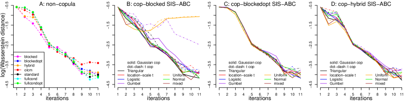
Figure 1: Two-moons model: median log-Wasserstein distances between the “exact”(MCMC) posterior and the ABC posteriors obtained via the guided or non-guided samplers across ten independent estimations. Panel A: non-copula-based methods, both guided and non-guided. Panel B: cop-blocked; Panel C: cop-blockedopt; Panel D: cop-hybrid. The copula-based methods are derived using either Gaussian (solid lines) or t copulas (dot-dashed lines) for different marginals, as described in the legend.

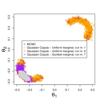
Figure 2: Two-moons model: 1,000 MCMC draws from the “exact”(MCMC) posterior (brown) and from the ABC posteriors obtained using the Gaussian-cop-blocked sampler with Gumbel marginals (purple, run number 7) and uniform marginals from run number 1 (grey) and 9 (orange). The 1,000 ABC draws obtained from copulas with uniform marginals cover the whole true posterior region only in some runs (here run 9), targeting a small sub-region of one of the two moons in most of the cases (here the first run), while those from the Gumbel marginals cover a larger sub-region of one of the two moons only in one run, successfully covering both moons in the other runs.

Acceptance rates are reported in Figure 3, and appear very stable across the ten runs, except for cop-blocked with uniform marginals. As also observed in Filippi et al. (2013), olcm is superior to standard in terms of acceptance rate, but both are outperformed across all iterations by all our novel guided methods except fullcondopt which is better than standard but slightly worse than olcm. Importantly, differences between the acceptance rates are large in early iterations, which is where the samples are still very dispersed in the posterior surface. Our methods are of great help in this case, as we wish to spend the least time possible to rule out initial “bad” particles, which is especially relevant for models that are computationally intensive to simulate. When we consider the wallclock running times, Figure 4 reveals that olcm requires way more time than any guided method to accept a particle (without improving the final inference though), and the guided fullcond, block, blockedopt and hybrid methods are the fastest in accepting particles. Overall, on our desktop machine (Intel Core i7-7700 CPU 3.60GHz 32 GB RAM) and without using any parallelization, the inference across the ten runs was completed in 5.5 minutes (with blocked), 5.4 minutes (blockedopt), 5.7 minutes (hybrid), 4.8 minutes (fullcond), 17.7 minutes (fullcondopt), 38.7 minutes (olcm) and 23.6 (20.8) minutes (standard). These are major time-differences given that this model is particularly simple to simulate. Copula methods are intrinsically slower in simulating proposals due to the more involved construction of a generic copula sampler and the less optimized numerical libraries compared to those implementing multivariate Gaussian samplers, independently on whether the codes are run in, say, R or Matlab (e.g. the Gaussian-cop-blocked, Gaussian-cop-blockedopt and Gaussian-cop-hybrid with normal marginals take 8.1, 11.4 and 9.4 minutes, instead of 5.5, 5.4 and 5.7 minutes of the corresponding blocked, blockedopt and hybrid). Since the acceptance rates of the guided-copula samplers are similar to those of the guided Gaussian samplers, the wallclock times of the former will become lower than the alternative non-guided samplers should the implementation of the R/Matlab copula built-in routines be improved (which is outside the scope of this work).

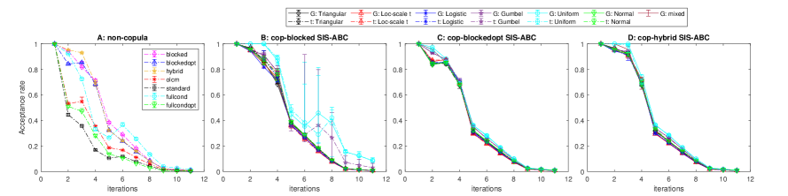
Figure 3: Two-moons model: median acceptance rates and error bars with first and third quartile across ten independent runs at each iteration. Panel A: Non-copula based methods, both guided and non-guided; Panel B: cop-blocked; Panel C: cop-blockedopt; Panel D: cop-hybrid. The copula-based methods are derived using either Gaussian (G, solid lines) or t copulas (dot-dashed lines) for different marginals, as described in the legend.

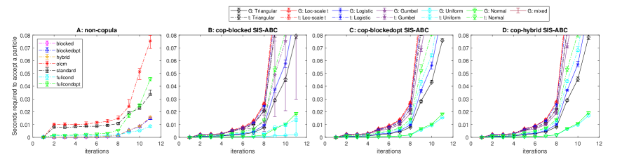
Figure 4: Two-moons model: median number of seconds required to accept a particle and error bars with first and third quartile across ten independent runs at each iteration. Panel A: Non-copula based methods, both guided and non-guided; Panel B: cop-blocked; Panel C: cop-blockedopt; Panel D: cop-hybrid. The copula-based methods are derived using either Gaussian (G, solid lines) or t (dot-dashed lines) copulas for different marginals, as described in the legend.

4.2 Twisted-prior model with an highly correlated posterior

We now consider a model with a challenging posterior characterised by a strong correlation between some of the parameters. This case study is particularly interesting, as the likelihood only provides location information about the unknown parameter while the dependence structure in the posterior comes mostly from the prior. For this reason, the posterior dependence changes direction depending on whether the likelihood locates the posterior in the left or right tail of the prior (see Nott et al., 2018 for a graphical illustration). This case study was analysed in an ABC context in Li et al. (2017). The model assumes observations $y=(y_{1},...,y_{d_{\theta}})$ drawn from a $d_{\theta}$-dimensional Gaussian $y\sim\mathcal{N}(\theta,\Psi)$, with $\theta=(\theta_{1},...,\theta_{d_{\theta}})$ and diagonal covariance matrix $\Psi=\mathrm{diag}(\sigma_{0},...,\sigma_{0})$. The prior is the “twisted-normal” prior of Haario et al. (1999), with density function proportional to $\pi(\theta)\propto\exp\biggl{\{}-\theta_{1}^{2}/200-(\theta_{2}-b\theta_{1}^{2}+100b)^{2}/2-\mathbbm{1}_{\{d_{\theta}>2\}}\sum_{j=3}^{d_{\theta}}\theta_{j}^{2}\biggr{\}},$ where $\mathbbm{1}_{B}$ denotes the indicator function of the set $B$. This prior is essentially a product of independent Gaussian distributions with the exception that the component for $(\theta_{1},\theta_{2})$ is modified to produce a “banana shape”, with the strength of the bivariate dependence determined by the parameter $b$. Simulation from $\pi(\theta)$ is achieved by first drawing $\theta$ from a $d_{\theta}$-dimensional multivariate Gaussian as $\theta\sim\mathcal{N}(0,A)$, where $A=\mathrm{diag}(100,1,...,1)$, and then placing the value $\theta_{2}+b\theta_{1}^{2}-100b$ in the slot for $\theta_{2}$. We consider a value for $b$ that induces a strong correlation in the prior between the first two components of $\theta$. Specifically, we use the same setup as Li et al. (2017), namely $\sigma_{0}=1$, $b=0.1$ and $d_{\theta}=5$, i.e. both $y_{\mathrm{obs}}$ and $\theta$ have length five, with observations given by the vector $y_{\mathrm{obs}}=(10,0,0,0,0)$. We take the identity function as summary statistic, i.e. $S(y)=y$, set an initial $\delta_{1}=50$ and let $\delta_{t}$ automatically decrease across iterations by taking $\psi=1$ (first percentile of the distances), as described at the beginning of Section 4, until the updated $\delta$ value gets smaller than 0.25, when the inference is then stopped.

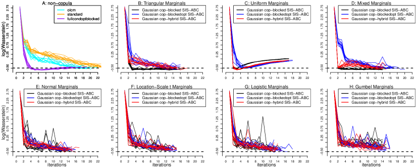
Figure 5: Twisted model: median log-Wasserstein distances between the “exact” posterior (MCMC) and the ABC posteriors across ten independent runs. Panel A: non-copula based methods, both guided (fullcondopt with $(\theta_{1},\theta_{2}$) blocked) and non-guided (olcm, standard); Panels B-H: guided Gaussian copula-based methods with triangular (B), uniform (C), “mixed” (D), normal (E), location-scale Student’s t (F), logistic (G) and Gumbel (H) marginals. The dashed lines mark a log-distance value of -0.5 (an arbitrary value only meant to ease eye-comparisons). Some runs are shorter than others depending on how many iterations $t$ it took to reach a value of $\delta_{t}$ smaller than 0.25. The results for the t copula-based samplers are almost indistinguishable to whose based on Gaussian copulas, and are thus not reported.

Low values of the ESS for some of the guided-methods (see the Supplementary Material F.2) are responsible for a larger variability between different runs, as in this case only few particles are resampled at the last iteration, and these appear to differ between runs. Instead, the ESS of the guided SMC-ABC fullcondoptblocked (Panel A), the guided SIS-ABC cop-blocked with triangular (Panel B) or mixed marginals (Panel D), or the guided-copulas with uniform marginals (Panel C) are higher than the non-guided ones (see the Supplementary Material F.2), being then less sensible to variability across independent runs. However, the distances obtained from marginal uniforms increase with the iterations as the consequence of the method becoming somehow overconfident, as illustrated in the Supplementary Material F.2, where the contour plots of the ABC posteriors at the last iteration of $(\theta_{1},\theta_{2})$ are reported. As for the two-moons study, this can be solved by considering mixed marginals (Panel D). Similar increasing distances happen also to fullcondoptblocked. Deriving a “sanity check”to prevent this deterioration in the inference performance, while of interest, is out of the scope of this work. However, a possible suggestion would be to stop the methods once the acceptance rate becomes lower than $1.5\%$ for two consecutive iterations (similarly to Del Moral et al., 2012), as it is unlikely that the inference will improve while the computational cost will increase. Additional results using this stopping criterion are in the Supplementary Material F.2, showing, indeed, an improved inference. Among all methods, for this case study we recommend using cop-blocked with either mixed or triangular marginals, as they have the merits of being robust across several runs and, more importantly, having small log-Wasserstein distances starting from as little as two or three iterations, respectively, with the mixed marginals having also higher acceptance rates at iteration two.

Figure 6: Schematic representation of the hierarchical g-and-k model.

4.3 Hierarchical g-and-k model with high-dimensional summaries

We now consider a high-dimensional model from Clarté et al. (2021). This is a hierarchical version of the g-and-k model, with the latter being often used as a toy case study in simulation-based inference (e.g. Fearnhead and Prangle, 2012), since its probability density function is unavailable in closed-form but it is possible to simulate from its quantile function. The g-and-k distribution is used to model non-standard data through five parameters $\theta=(A,B,g,k,c)$, though in practice $c$ is often fixed to 0.8 (Prangle, 2020), as we do here. Details about simulating $x\sim gk(A,B,g,k)$ from a g-and-k distribution are in the Supplementary Material G. Same as Clarté et al. (2021), we assume to have observations $x_{ij}$ ($i=1,...,n,j=1,...,J$) sampled from a hierarchical g-and-k model, where each $J$-dimensional vector $x_{i}=(x_{i1},...,x_{iJ})$ is characterised by its own parameter $A_{i}$, while $(B,g,k)$ are common to all $n$ units and are assumed known. We assume $A_{i}\sim\mathcal{N}(\alpha,1)$ for $\alpha$ unknown and $x_{ij}\sim gk(A_{i},B,g,k)$, see Figure 6. We also assume $\alpha\sim\mathrm{Unif}(-10,10)$ and, ultimately, we infer $\theta=(\alpha,A_{1},...,A_{n})$. Here, we generate data with $n=20$ and $J=1,000$ by using $(B,g,k,\alpha)=(0.192,0.622,0.438,5.707)$. Same as Clarté et al. (2021), summary statistics for $x_{i}$ are the vector of nine quantiles $\mathrm{quant}(x_{i},l/8)$ ($l=0,1,...,8$), where $\mathrm{quant}(x,p)$ is the $p$-th quantile of sample $x$. This setting leads to a challenging inference problem for ABC, as the vector $\theta$ to infer is 21-dimensional and summary statistics are a vector of length $9n=180$.
Since an exact posterior is not available here, we obtain 1,000 posterior samples from the ABC-Gibbs sampler of Clarté et al. (2021) to produce a “reference posterior”, as this method is designed (and thus especially suited) for hierarchical models. Here, our focus is on comparing the performance (with respect to the reference ABC-Gibbs) and running times of $N=10^{4}$ draws sampled from our proposed guided hybrid and cop-hybrid SIS-ABC versus the SMC-ABC olcm and standard. For sequential ABC methods, we set an initial $\delta_{1}=50$ and let $\delta_{t}$ automatically decrease across iterations as described at the beginning of Section 4 by taking $\psi=25$ (25-th percentile of all simulated distances), stopping the methods as soon as the updated $\delta$ value gets smaller than 0.62. However, most methods did not manage to reach this value in reasonable time and had to be halted, as the number of seconds required to accept a particle became rapidly larger than that of hybrid, which succeeds in drastically decreasing the threshold $\delta_{t}$ at iteration 3 compared to the non-guided approaches, see the Supplementary Material G. In terms of running times, the non-guided standard was very slow, with 14.5 million model simulations (for a single run) to attain a threshold around $2.14$ in 42 hours (at iteration $t=26$). Moreover, standard resulted in quite uninformative marginal posteriors for the $A_{i}$ parameters, see Figure 7 (for ease of display, we only report the ABC posteriors of $\alpha$ and $A_{1},...,A_{5}$). Hence, not much is being learned except for $\alpha$, despite the large number of simulations. On the contrary, hybrid locates the high posterior mass region with higher precision and much more rapidly. In each of the ten runs, hybrid reached $\delta=0.62$ with $9\cdot 10^{5}-1\cdot 10^{6}$ model simulations in 2–3 hours, a speedup of at least fourteen times compared to standard. In fact, the total speedup is likely to be much larger, as we do not know how longer standard should have run to reach satisfying inference. Notice that, for this example, the guided hybrid is plagued by a very small ESS (see the Supplementary Material G), so the posterior variability is different between runs. A possibility to tackle this may be to incorporate guided proposal samplers into the SMC-ABC of Del Moral et al. (2012) (or vice versa), which is designed to progressively, albeit slowly, reduce $\delta$ while maintaining a reasonably high ESS value. Doing this would, on the one hand, open some theoretical questions (e.g. whether the resulting proposal kernel satisfies the detailed balance equation) and, on the other hand, introduce a MCMC step which would modify all weights, something which goes beyond the scope of this work. Note however that, despite the low ESS in this example, the bulk of the posteriors resulting from hybrid resembles that from the ABC-Gibbs method. The non-guided olcm yields more satisfactory results than standard (see the Supplementary Material G), but the corresponding threshold value after 1 million model simulations was still $\delta=1.87$, so it was still fairly spread compared to hybrid. Moreover, olcm took about 55 hours to reach $\delta=0.70$ compared to about 2–3 hours for hybrid to reach $\delta=0.62$, with a median speedup of 20 times. ABC-Gibbs was the fastest one (with a running time of 30 minutes), which is not surprising, as that scheme is especially suited for hierarchical models.

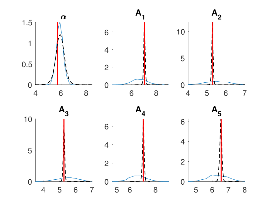
(a) standard

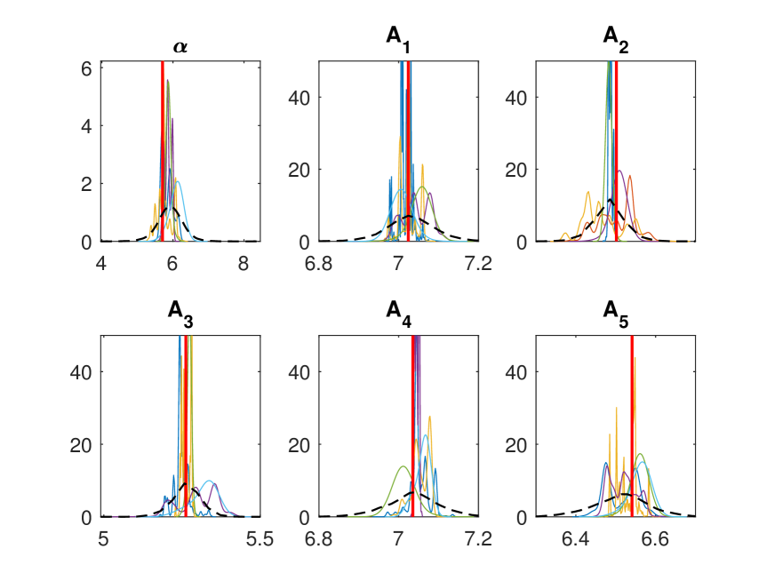
(b) hybrid

Figure 7: Hierarchical g-and-k model: posteriors displayed only for $(\alpha,A_{1},...,A_{5})$, using: (a) standard at iteration $t=26$ and $\delta=2.14$ after $14.5\cdot 10^{6}$ model simulations; (b) five inference runs of hybrid, all reaching $\delta=0.62$ in approximately $10^{6}$ model simulations per run. Dashed lines are posteriors from ABC-Gibbs. Red vertical lines mark ground-truth values.

4.4 Recruitment boom-and-bust model with highly skewed summaries

We now challenge our guided proposals samplers, whose non-copula (more precisely, non-$t$-copula) approaches have been constructed assuming joint normality of the particle pairs $(\theta,s)$, on another example characterised by highly non-Gaussian summary statistics, namely, the recruitment boom-and-bust model. This is a stochastic discrete time model which may be used to describe the fluctuation of population sizes over time. The model is characterised by four parameters $\theta=(r,\kappa,\alpha,\beta)$, with small values of $\beta$ (as used here to generate our data) giving rise to highly non-Gaussian summary statistics. This case study, which we fully describe and analyze in the Supplementary Material H, was also considered in Fasiolo et al. (2018), An et al. (2020) and Picchini et al. (2022) in the context of MCMC via synthetic likelihood, to test how that methodology, constructed under approximately Gaussian distributed summary statistics, performed. As a reference gold-standard posterior is unavailable, here we compare guided and non-guided ABC approaches with the robustified semiparametric (Bayesian) synthetic likelihood approach of An et al. (2020), denoted semiBSL. Note that this case study uses twelve summary statistics, three times as many as the number of parameters to infer, a setting where ABC is expected to struggle with its curse-of-dimensionality. In fact, the ABC posteriors are more spread than the posterior returned by semiBSL, which concentrates around the true parameter values thanks to its (semi)parametric nature. Among our proposed approaches, guided methods without “optimised” covariances occasionally appear mode-seeking, as discussed and observed elsewhere. However, some of the copula-methods (notably Gaussian copulas with triangular marginals) behave quite similarly to semiBSL. More generally, guided approaches show higher acceptance rates, similar (if not better) performances and quicker runtimes than the considered traditional non-guided ABC approaches.

4.5 Cell motility and proliferation with high-dimensional summaries

Finally, we consider a simulated, yet realistic, study of cell movements characterised by high dimensional summary statistics, a well-known challenge for ABC. We initially considered 145 summary statistics, then 289 and finally 433. Model details and inferential results are reported in the Supplementary Material I. The main take away is that guided and non-guided SMC-ABC are able to deal with such large dimensionalities, whereas for summaries of size 289 (and larger), the Bayesian synthetic likelihood MCMC sampler of Price et al. (2018) (the original version, we did not consider more recent developments) was unable to mix even for starting parameters set at the ground truth values. With guided and non-guided SMC-ABC, we managed to perform inference using summaries with up to dimension 433, with the former requiring many fewer model simulations than the latter. This is particularly remarkable, as all proposed guided samplers require the inversion of possibly high-dimensional covariance matrices of summary statistics (in (4), (5), (9), (10)), something which is known to be both numerically challenging and computationally expensive. Hence, not only the proposed schemes can successfully handle such inversion, but they are as fast as the non-guided proposals which do not require it.

5 Discussion

We introduced a range of multivariate Gaussian and copula-based (both Gaussian and t copulas, with six considered distributions of the marginals of the copula) proposal samplers to accelerate inference when using sequential ABC methods, notably sequential importance sampling (SIS-ABC) and sequential Monte Carlo (SMC-ABC). The acceleration is implied by the construction of proposal samplers that are made conditional to the summary statistics of the data (which is why we called them “guided”), such that the proposed draws rapidly converge to the bulk of the posterior distribution. We challenged our samplers by considering posteriors with multimodal surfaces (two-moons, Section 4.1), highly non-Gaussian summary statistics (two-moons, Section 4.1 and recruitment boom-and-bust, Section 4.4), high dimensional parameter space (hierarchical g-and-k, Section 4.3), high dimensional summaries with hundreds of components (hierarchical g-and-k, Section 4.3 and cell motility model, Section 4.5), and highly correlated posteriors (twisted model, Section 4.2). In all these case studies, on the one hand, our methods obtained satisfactory ABC inference, similar, if not better, to non-guided sequential ABC schemes, in particular compared to the most commonly implemented proposal sampler (found in all the most used ABC software packages and papers considering SMC-ABC), which in fact we named standard (Beaumont et al., 2009, but we also extensively compared with the olcm sampler of Filippi et al., 2013). On the other hand, thanks to being guided, they returned inference much more rapidly than the non-guided proposal samplers. In particular, for a fast to simulate generative model with a low-dimensional parameter space (two-moons, Section 4.1), our methods were already 4–6 times faster than customary non-guided SMC-ABC schemes, suggesting the possibility of even higher accelerations for more expensive simulators and/or higher dimensional parameter/summary statistics spaces. This was indeed observed in a challenging case study (hierarchical g-and-k model, Section 4.3), where the non-guided SMC-ABC sampler standard, which is the typical default option in most software implementing SMC-ABC, was at least fourteen times slower than our guided ABC samplers in approaching a gold-standard ABC posterior. For guided methods showing ESS lower than standard and olcm, the corresponding “optimised” version managed to considerably increase the ESS values.
Among the introduced guided samplers, the copula-based samplers are general and flexible. Among them, those based on Gaussian copulas may be preferred, yielding higher ESS values (for some marginals higher than the non-copula guided samplers) and being slightly faster than the $t$ copulas, while yielding similar performances. However guided non-copula Gaussian samplers are also competitive, and perform notably better than the non-guided samplers. Overall, the best copula-based sampler is the cop-blocked with triangular or mixed marginal distributions, followed by either cop-blockedopt or cop-hybrid with uniform marginals. However, copula-based samplers involve more operations to produce a proposal and may use less optimized numerical libraries compared to multivariate Gaussian samplers. This difference is negligible if the model simulator is expensive, as in this case the computational bottleneck will be the forward model simulation, but may be less so for particularly simple simulators (e.g. the two-moons), for which the copula-based samplers may then be slower than the guided multivariate Gaussians. This is not a disadvantage if the geometry of the posterior is such that the copula-model better adapts to its exploration, as it happens for the twisted model (for cop-blocked with triangular marginals).
The proposed approach opens to a number of possible avenues of investigation, e.g. guided copula-based SMC-ABC samplers, non-parametric guided copula-based samplers, where the copula and the marginals are fitted non-parametrically from the available data, or “fully” copula-based sequential samplers, where a copula is placed on $(\theta,s)$ instead of $\theta|s$. Embedding our guided proposals into ensemble Kalman inversion (EKI, see Chada, 2022 for a recent review) would also be of interest. Overall, our guided proposals are easy to construct and are rapidly computed from accepted parameters and summary statistics, thus not introducing any substantial overhead. For example, there is no need to construct and train a deep neural network (unlike in the guided method of Chen and Gutmann, 2019), or perform a high-dimensional non-parametric optimization. We believe that the simplicity, and effectiveness, of our proposal samplers makes them appealing and easy to incorporate into the user’s toolbox.

Supplementary Material

The supplementary material contains both additional methodological details (e.g. the construction of the optimized covariance matrices $\Sigma_{t}$ (7) and optimized variances $\sigma^{*2}_{k}$ (13), the derivation of the underlying parameters of the marginal distributions for the guided copula-based SIS-ABC sampler), and further results/figures for the considered simulation studies.

Acknowledgments

UP acknowledges support from the Swedish Research Council (Vetenskapsrådet 2019-03924) and the Chalmers AI Research Centre (CHAIR).

See pages - of supplementary.pdf

References

- Alsing et al. [2018] J. Alsing, B. D. Wandelt, and S. M. Feeney. Optimal proposals for approximate Bayesian computation. arXiv:1808.06040, 2018.
- An et al. [2020] Z. An, D. J. Nott, and C. Drovandi. Robust Bayesian synthetic likelihood via a semi-parametric approach. Statistics and Computing, 30:543–557, 2020.
- Beaumont et al. [2002] M. A. Beaumont, W. Zhang, and D. J. Balding. Approximate Bayesian computation in population genetics. Genetics, 162(4):2025–2035, 2002.
- Beaumont et al. [2009] M. A. Beaumont, J.-M. Cornuet, J.-M. Marin, and C. P. Robert. Adaptive approximate Bayesian computation. Biometrika, 96(4):983–990, 2009.
- Bedford and Cooke [2002] T. Bedford and R. M. Cooke. Vines: A new graphical model for dependent random variables. Annals of Statistics, 30:1031–1068, 2002.
- Blum and François [2010] M. G. Blum and O. François. Non-linear regression models for approximate Bayesian computation. Statistics and computing, 20(1):63–73, 2010.
- Bonassi and West [2015] F. Bonassi and W. West. Sequential monte carlo with adaptive weights for approximate bayesian computation. Bayesian Analysis, 1:171–187, 2015.
- Cappé et al. [2004] O. Cappé, A. Guillin, J.-M. Marin, and C. P. Robert. Population Monte Carlo. Journal of Computational and Graphical Statistics, 13(4):907–929, 2004.
- Chada [2022] N. K. Chada. A review of the EnKF for parameter estimation. In Inverse Problems - Recent Advances and Applications. IntechOpen, 2022. doi: 10.5772/intechopen.108218.
- Chen and Shao [1999] M.-H. Chen and Q.-M. Shao. Monte Carlo estimation of Bayesian credible and HPD intervals. Journal of Computational and Graphical Statistics, 8(1):69–92, 1999.
- Chen and Gutmann [2019] Y. Chen and M. U. Gutmann. Adaptive Gaussian copula ABC. In The 22nd International Conference on Artificial Intelligence and Statistics, pages 1584–1592. PMLR, 2019.
- Clarté et al. [2021] G. Clarté, C. P. Robert, R. J. Ryder, and J. Stoehr. Componentwise approximate Bayesian computation via Gibbs-like steps. Biometrika, 108(3):591–607, 2021.
- Del Moral et al. [2006] P. Del Moral, A. Doucet, and A. Jasra. Sequential Monte Carlo samplers. Journal of the Royal Statistical Society: Series B (Statistical Methodology), 68(3):411–436, 2006.
- Del Moral et al. [2012] P. Del Moral, A. Doucet, and A. Jasra. An adaptive sequential Monte Carlo method for approximate Bayesian computation. Statistics and computing, 22(5):1009–1020, 2012.
- Duffield and Singh [2022] S. Duffield and S. S. Singh. Ensemble Kalman inversion for general likelihoods. Statistics & Probability Letters, 187:109523, 2022.
- Dutta et al. [2017] R. Dutta, M. Schoengens, L. Pacchiardi, A. Ummadisingu, N. Widmer, J.-P. Onnela, and A. Mira. ABCpy: A high-performance computing perspective to approximate Bayesian computation. Journal of Statistical Software, 100:1–38, 2017.
- Embrechts et al. [2002] P. Embrechts, A. McNeil, and D. Straumann. Correlation and dependence in risk management: properties and pitfalls. In Risk Management: Value at Risk and Beyond, pages 176–223. Cambridge University Press, 2002.
- Fasiolo et al. [2018] M. Fasiolo, S. N. Wood, F. Hartig, M. V. Bravington, et al. An extended empirical saddlepoint approximation for intractable likelihoods. Electronic Journal of Statistics, 12(1):1544–1578, 2018.
- Fearnhead and Prangle [2012] P. Fearnhead and D. Prangle. Constructing summary statistics for approximate Bayesian computation: semi-automatic approximate Bayesian computation. Journal of the Royal Statistical Society: Series B (Statistical Methodology), 74(3):419–474, 2012.
- Filippi et al. [2013] S. Filippi, C. P. Barnes, J. Cornebise, and M. P. Stumpf. On optimality of kernels for approximate Bayesian computation using sequential Monte Carlo. Statistical applications in genetics and molecular biology, 12(1):87–107, 2013.
- Greenberg et al. [2019] D. Greenberg, M. Nonnenmacher, and J. Macke. Automatic posterior transformation for likelihood-free inference. In International Conference on Machine Learning, pages 2404–2414. PMLR, 2019.
- Haario et al. [1999] H. Haario, E. Saksman, and J. Tamminen. Adaptive proposal distribution for random walk Metropolis algorithm. Computational Statistics, 14(3):375–395, 1999.
- Higham [1988] N. J. Higham. Computing a nearest symmetric positive semidefinite matrix. Linear algebra and its applications, 103:103–118, 1988.
- Hoeffding [1940] W. Hoeffding. Massstabinvariante korrelationstheorie. Schriften des Mathematischen Seminars und des Instituts fur Angewandte Mathematik der Universitat Berlin, page 181–233, 1940.
- Li et al. [2017] J. Li, D. J. Nott, Y. Fan, and S. A. Sisson. Extending approximate Bayesian computation methods to high dimensions via a Gaussian copula model. Computational Statistics & Data Analysis, 106:77–89, 2017.
- Lueckmann et al. [2017] J.-M. Lueckmann, P. J. Goncalves, G. Bassetto, K. Öcal, M. Nonnenmacher, and J. H. Macke. Flexible statistical inference for mechanistic models of neural dynamics. arXiv:1711.01861, 2017.
- Lueckmann et al. [2021] J.-M. Lueckmann, J. Boelts, D. S. Greenberg, P. J. Gonçalves, and J. H. Macke. Benchmarking simulation-based inference. In The 24th International Conference on Artificial Intelligence and Statistics, volume 130, pages 343–351. PMLR, 2021.
- Marjoram et al. [2003] P. Marjoram, J. Molitor, V. Plagnol, and S. Tavaré. Markov chain Monte Carlo without likelihoods. Proceedings of the National Academy of Sciences, 100(26):15324–15328, 2003.
- Martino et al. [2017] L. Martino, V. Elvira, and F. Louzada. Effective sample size for importance sampling based on discrepancy measures. Signal Processing, 131:386–401, 2017.
- Nott et al. [2018] D. J. Nott, V. M.-H. Ong, Y. Fan, and S. Sisson. Handbook of approximate Bayesian computation, chapter High-dimensional ABC. Chapman and Hall/CRC, 2018.
- Papamakarios and Murray [2016] G. Papamakarios and I. Murray. Fast -free inference of simulation models with bayesian conditional density estimation. In Advances in neural information processing systems, pages 1028–1036, 2016.
- Papamakarios et al. [2019] G. Papamakarios, D. Sterratt, and I. Murray. Sequential neural likelihood: Fast likelihood-free inference with autoregressive flows. In The 22nd International Conference on Artificial Intelligence and Statistics, pages 837–848. PMLR, 2019.
- Picchini [2014] U. Picchini. Inference for SDE models via approximate Bayesian computation. Journal of Computational and Graphical Statistics, 23(4):1080–1100, 2014.
- Picchini et al. [2022] U. Picchini, U. Simola, and J. Corander. Sequentially guided MCMC proposals for synthetic likelihoods and correlated synthetic likelihoods. Bayesian Analysis, 2022. doi: 10.1214/22-BA1305.
- Prangle [2020] D. Prangle. gk: An R package for the g-and-k and generalised g-and-h distributions. The R journal, 12:7–20, 2020.
- Price et al. [2018] L. F. Price, C. C. Drovandi, A. Lee, and D. J. Nott. Bayesian synthetic likelihood. Journal of Computational and Graphical Statistics, 27(1):1–11, 2018.
- Pritchard et al. [1999] J. K. Pritchard, M. T. Seielstad, A. Perez-Lezaun, and M. W. Feldman. Population growth of human y chromosomes: a study of y chromosome microsatellites. Molecular biology and evolution, 16(12):1791–1798, 1999.
- Schuhmacher et al. [2020] D. Schuhmacher, B. Bähre, C. Gottschlich, V. Hartmann, F. Heinemann, and B. Schmitzer. transport: Computation of Optimal Transport Plans and Wasserstein Distances, 2020. URL https://cran.r-project.org/package=transport. R package version 0.12-2.
- Schälte et al. [2022] Y. Schälte, E. Klinger, E. Alamoudi, and J. Hasenauer. pyABC: Efficient and robust easy-to-use approximate bayesian computation. Journal of Open Source Software, 7:4304, 2022.
- Sisson and Fan [2011] S. A. Sisson and Y. Fan. Handbook of Markov chain Monte Carlo, chapter Likelihood-free MCMC. Chapman & Hall/CRC, New York., 2011.
- Sisson et al. [2007] S. A. Sisson, Y. Fan, and M. M. Tanaka. Sequential Monte Carlo without likelihoods. Proceedings of the National Academy of Sciences, 104(6):1760–1765, 2007.
- Sisson et al. [2018] S. A. Sisson, Y. Fan, and M. Beaumont. Handbook of Approximate Bayesian Computation. Chapman and Hall/CRC, 2018.
- Sklar [1959] M. Sklar. Fonctions de répartition á n dimensions et leurs marges. Inst. Stat. Univ. Paris, 8:229–231, 1959.
- Sommerfeld and Munk [2018] M. Sommerfeld and A. Munk. Inference for empirical wasserstein distances on finite spaces. Journal of the Royal Statistical Society: Series B (Statistical Methodology), 80(1):219–238, 2018.
- Toni et al. [2008] T. Toni, D. Welch, N. Strelkowa, A. Ipsen, and M. P. Stumpf. Approximate Bayesian computation scheme for parameter inference and model selection in dynamical systems. Journal of the Royal Society Interface, 6(31):187–202, 2008.
- Wiqvist et al. [2021] S. Wiqvist, J. Frellsen, and U. Picchini. Sequential neural posterior and likelihood approximation. arXiv preprint arXiv:2102.06522, 2021.
- Wood [2010] S. N. Wood. Statistical inference for noisy nonlinear ecological dynamic systems. Nature, 466(7310):1102–1104, 2010.