This paper has been accepted for publication in IEEE Robotics and Automation Letters.

This is the author’s version of an article that has, or will be, published in this journal or conference. Changes were, or will be, made to this version by the publisher prior to publication.

DOI:	10.1109/LRA.2022.3179424
IEEE Xplore:	https://ieeexplore.ieee.org/document/9786679

Please cite this paper as:

T. Hitchcox and J. R. Forbes, “Mind the Gap: Norm-Aware Adaptive Robust Loss for Multivariate Least-Squares Problems,” in IEEE Robotics and Automation Letters, vol. 7, no. 3, pp. 7116-7123, 2022.

©2022  IEEE. Personal use of this material is permitted. Permission from IEEE must be obtained for all other uses, in any current or future media, including reprinting/republishing this material for advertising or promotional purposes, creating new collective works, for resale or redistribution to servers or lists, or reuse of any copyrighted component of this work in other works.

Mind the Gap: Norm-Aware Adaptive Robust Loss for Multivariate Least-Squares Problems

Abstract

Measurement outliers are unavoidable when solving real-world robot state estimation problems. A large family of robust loss functions (RLFs) exists to mitigate the effects of outliers, including newly developed adaptive methods that do not require parameter tuning. All of these methods assume that residuals follow a zero-mean Gaussian-like distribution. However, in multivariate problems the residual is often defined as a norm, and norms follow a Chi-like distribution with a non-zero mode value. This produces a “mode gap” that impacts the convergence rate and accuracy of existing RLFs. The proposed approach, “Adaptive MB,” accounts for this gap by first estimating the mode of the residuals using an adaptive Chi-like distribution. Applying an existing adaptive weighting scheme only to residuals greater than the mode leads to more robust performance and faster convergence times in two fundamental state estimation problems, point cloud alignment and pose averaging.

I Introduction

Measurement outliers occur in state estimation problems due to erroneous sensor measurements [1] or faulty data association decisions [2]. Outliers degrade state-estimation solution accuracy, as residuals formed from outlier measurements can have an outsized impact when attempting to minimize an objective function. To address this, a large family of robust loss functions (RLFs) may be used to modify the objective function in a way that downweights residuals caused by outliers. Popular RLFs in the literature include pseudo-Huber (also referred to as L1-L2) [3, 4], Cauchy [5], Geman-McClure [6], and Welsch [7] loss, with each RLF defining a distribution on the residual weights (see Figure 1).

The drawback to these conventional RLFs is that they must be selected and tuned a priori, without knowledge of how the residuals are actually distributed. To address this, [8] developed an adaptive loss function that adjusts to the shape of the residual distribution, eliminating the need for model selection and tuning. This method was recently extended in [9], which made the RLF capable of adapting to a wider range of distributions.

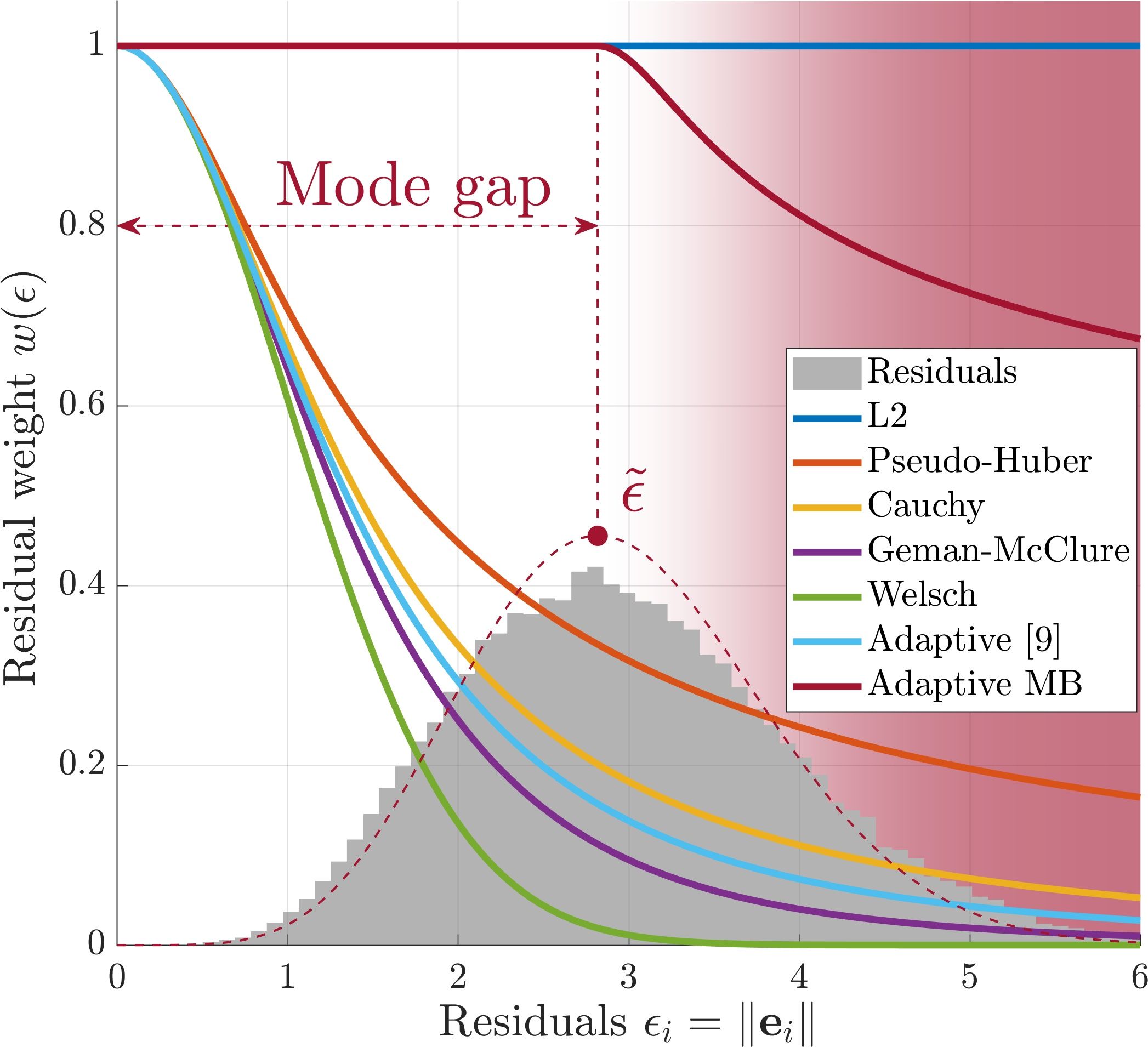
Figure 1: In multivariate least-squares problems, residuals are often defined as norms. If $\mbf{e}_{i}$ is normally distributed, residual ${\epsilon_{i}=\|\mbf{e}_{i}\|}$ will follow a Chi distribution with mode $\tilde{\epsilon}$. The proposed robust loss function, “Adaptive MB,” accounts for this “mode gap” when assigning residual weights. As a result, ${w_{i}<1}$ only in the outlier region (red), leading to more robust performance and faster convergence when outliers are present.

However, all existing RLFs assume a Gaussian-like distribution with a mode of zero, and weight highly residuals with a low magnitude. This is visualized in Figure 1 by the family of weighting functions that peak at zero. However, residuals are often defined as the norm of a multivariate error, for example the Mahalanobis distance. If the error follows a Gaussian-like distribution, then it’s norm will follow a Chi-like distribution with a mode value $\tilde{\epsilon}$ greater than zero. This leads to the development of a “mode gap,” shown in Figure 1, which can inadvertently influence the weighting scheme.

In Figure 1, residuals less than the mode value are clearly inliers, as they are expected to be observed given the statistics on error $\mbf{e}_{i}$. When they occur, outliers will produce residual values far greater than $\tilde{\epsilon}$, in the red region of Figure 1. However, due to the mode gap, both inliers and outliers receive a moderate to low weight from RLFs that assume a mode of zero. Ambiguous weighting between inliers and outliers will lead to slower convergence behaviour and less accurate results, especially if the mode gap grows larger or if the selected RLF is more conservative, for example Welsch loss.

The method proposed here, called “Adaptive MB,” accounts for this gap by first estimating the mode value by fitting an $n$-dimensional Maxwell-Boltzmann (MB) distribution to the residuals. An MB distribution is a generalization of the Chi distribution, with a shape parameter that allows for flexibility during the fitting process. Accounting for the mode gap, a weight of ${w_{i}=1}$ is assigned to residuals less than the mode, which are assumed to be inliers, and the adaptive method from [9] is applied to residuals greater than the mode, where outliers actually reside. The primary contribution of this work is in acknowledging and responding to this gap, and represents a novel insight in the study of outlier rejection [10].

The proposed method is tested against several fixed RLFs, as well as existing adaptive approaches [8, 9], on two fundamental state estimation problems, point cloud alignment and pose averaging. As predicted from the theory, accounting for the “mode gap” leads to more robust performance and faster convergence times in these applications.

II Preliminaries

II-A Robust Loss Functions

Optimization problems in state estimation often seek to minimize a sum of weighted squared residuals,

$$\mbf{x}^{\star}=\operatorname*{arg\,min}_{\mbf{x}\in\mathbb{R}^{N}}J(\mbf{x})=\operatorname*{arg\,min}_{\mbf{x}\in\mathbb{R}^{N}}\color[rgb]{0,0,0}{\frac{1}{2}}\color[rgb]{0,0,0}\sum^{N}_{i=1}w_{i}\cdot\color[rgb]{0,0,0}{\epsilon_{i}}\color[rgb]{0,0,0}\left(z_{i},g_{i}(x_{i})\right)\color[rgb]{0,0,0}{{}^{2}}\color[rgb]{0,0,0},\vspace{9pt}$$ (1)

where ${\mbf{x}\in\mathbb{R}^{N}}$ is the state vector, ${w_{i}\in\color[rgb]{0,0,0}{(}\color[rgb]{0,0,0}0,1]}$ are weights, and $\epsilon_{i}$ are residuals. The residuals are typically a function of sensor measurements $z_{i}$ and some nonlinear function $g_{i}(x_{i})$ of the current state estimate. Equation 1 is often solved within an iteratively reweighted least-squares (IRLS) framework [11], where the weights $w_{i}(\color[rgb]{0,0,0}{\epsilon_{i}}\color[rgb]{0,0,0}(\bar{x}_{i}))$ are evaluated at the current operating point $\bar{\mbf{x}}$. The objective function $J(\mbf{x})$ is then minimized by linearizing about $\bar{\mbf{x}}$ and applying, for example, Gauss-Newton or Levenberg-Marquardt [12, §4.3.1].

Robust loss functions modify the objective function in a way that downweights residuals caused by outliers. Incorporating robust loss $\rho(\color[rgb]{0,0,0}{\epsilon}\color[rgb]{0,0,0})$ into (1) produces a new objective function,

$$J_{\textrm{mod.}}(\mbf{x})=\sum^{N}_{i=1}\rho_{i}(\color[rgb]{0,0,0}{\epsilon_{i}}\color[rgb]{0,0,0}(x_{i})).\vspace{6pt}$$ (2)

Rather than minimize (2) directly, the weights $w_{i}$ in the original problem are obtained by equating the gradients,

$$\frac{\partial}{\partial x_{i}}J(\mbf{x})= \ w_{i}\color[rgb]{0,0,0}{\cdot}\color[rgb]{0,0,0}\color[rgb]{0,0,0}{\epsilon_{i}}\color[rgb]{0,0,0}(x_{i})\frac{\partial\color[rgb]{0,0,0}{\epsilon_{i}}\color[rgb]{0,0,0}(x_{i})}{\partial x_{i}},$$ (3a)

$$\frac{\partial}{\partial x_{i}}J_{\textrm{mod.}}(\mbf{x})= \ \frac{\partial\rho_{i}(\color[rgb]{0,0,0}{\epsilon_{i}}\color[rgb]{0,0,0}(x_{i}))}{\partial\color[rgb]{0,0,0}{\epsilon_{i}}\color[rgb]{0,0,0}(x_{i})}\frac{\partial\color[rgb]{0,0,0}{\epsilon_{i}}\color[rgb]{0,0,0}(x_{i})}{\partial x_{i}},$$ (3b)

and therefore

$$w_{i}=\frac{1}{\color[rgb]{0,0,0}{\epsilon_{i}}\color[rgb]{0,0,0}(x_{i})}\frac{\partial\rho_{i}(\color[rgb]{0,0,0}{\epsilon_{i}}\color[rgb]{0,0,0}(x_{i}))}{\partial\color[rgb]{0,0,0}{\epsilon_{i}}\color[rgb]{0,0,0}(x_{i})}.\vspace{6pt}$$ (4)

II-B An Adaptive Robust Loss Function

Recently, [8] developed an adaptive robust loss function, which dynamically adjusts to match the actual residual distribution. Defining the unitless residual value as the error scaled by a noise bound $c$,

$$\epsilon_{i}=\frac{e_{i}}{c},\vspace{3pt}$$ (5)

and accounting for singularities, the RLF is defined piecewise,

$$\rho(\epsilon,\alpha)=\begin{cases}\tfrac{1}{2}\epsilon^{2}&\text{if}\ \alpha=2,\\ \log\left(\tfrac{1}{2}\epsilon^{2}+1\right)&\text{if}\ \alpha=0,\\ 1-\exp\left(-\tfrac{1}{2}\epsilon^{2}\right)&\text{if}\ \alpha=-\infty,\\ \tfrac{|\alpha-2|}{\alpha}\left(\left(\frac{\epsilon^{2}}{|\alpha-2|}+1\right)^{\alpha/2}-1\right)&\text{otherwise},\end{cases}$$ (6)

where ${\alpha\in(-\infty,2]}$ is a shape parameter. To adapt (6), [8] assumes the following distribution on the residuals,

$$p(\epsilon\,|\,\mu,\alpha)=\frac{1}{Z(\alpha)}\exp\left(-\rho\left(\epsilon-\mu,\alpha\right)\right),\vspace{6pt}$$ (7)

where $\mu$ is the residual mean and $Z(\alpha)$ is a normalization constant. With ${\mu=0}$,

$$Z(\alpha)=\!\!\int^{\infty}_{-\infty}\exp\left(-\rho(\epsilon,\alpha)\right)\,\mathrm{d}\epsilon.\vspace{6pt}$$ (8)

The distribution (7) is therefore the likelihood of observing the residuals given shape parameter $\alpha$. The optimal $\alpha^{\star}$ is found by maximizing this likelihood, or alternatively by minimizing the negative log-likelihood. For a discrete set of residuals ${\{\epsilon_{i}\}^{N}_{i=1}}$,

$$\alpha^{\star}= \,\operatorname*{arg\,min}_{\alpha\in[0,2]}-\log\left(p(\epsilon\,|\,\alpha)\right)$$ (9a)

$$= \,\operatorname*{arg\,min}_{\alpha\in[0,2]}\Big{(}\underbrace{N\cdot\log(Z(\alpha))+\sum^{N}_{i=1}\rho_{i}(\epsilon_{i},\alpha)}_{\Lambda(\alpha)}\Big{)}.$$ (9b)

Having optimized the shape parameter, the weights ${w_{i}\in(0,1]}$ in the original optimization problem (1) are given by

$$w_{i}(\epsilon_{i},\alpha^{\star})=\begin{cases}1&\text{if}\ \alpha^{\star}=2,\\ \tfrac{1}{\nicefrac{{\epsilon^{2}_{i}}}{{2}}+1}&\text{if}\ \alpha^{\star}=0,\\ \exp\left(-\tfrac{1}{2}\epsilon^{2}_{i}\right)&\text{if}\ \alpha^{\star}=-\infty,\\ \left(\frac{\epsilon_{i}^{2}}{|\alpha^{\star}-2|}+1\right)^{\nicefrac{{\alpha^{\star}}}{{2}}-1}&\text{otherwise}.\end{cases}\vspace{3pt}$$ (10)

More recently, [9] noted that the optimization for $\alpha^{\star}$ in the original approach is limited to ${\alpha^{\star}\in[0,2]}$, as the integral in (8) is unbounded for ${\alpha<0}$. To address this, [9] truncates the distribution such that $-\tau\leq\epsilon\leq\tau$,

$$\tilde{p}(\epsilon\,|\,\alpha)= \ \frac{1}{\tilde{Z}(\alpha)}\exp\left(-\rho(\epsilon,\alpha)\right),$$ (11a)

$$\vspace{3pt}\tilde{Z}(\alpha)= \!\int^{\tau}_{-\tau}\exp\left(-\rho(\epsilon,\alpha)\right)\,\mathrm{d}\epsilon.$$ (11b)

In this work, the truncation bound $\tau$ is set according to the specifics of the problem, and is increased both when the magnitude of the residuals is expected to be large and when the dimension of the error increases. Using $\tilde{Z}(\alpha)$ in place of $Z(\alpha)$ in (9b), the optimal shape parameter $\alpha^{\star}$ is found here using Newton’s method with a backtracking line search, with

$$\frac{\mathrm{d}}{\mathrm{d}\alpha}\Lambda(\alpha)=-\frac{N}{\tilde{Z}(\alpha)}\int^{\tau}_{-\tau}\exp(-\rho(\epsilon,\alpha))\frac{\partial\rho}{\partial\alpha}\mathrm{d}\epsilon+\sum^{N}_{i=1}\frac{\partial\rho_{i}}{\partial\alpha}.$$ (12)

This was found to halve the execution time over the grid search method originally used in [9].

III Methodology

III-A Defining Residuals in Multivariate Least-Squares Problems

More often, state estimation problems seek to minimize a sum of weighted, squared multivariate errors,

$$J(\mbf{X})=\frac{1}{2}\sum^{N}_{i=1}\color[rgb]{0,0,0}{w_{i}\cdot}\color[rgb]{0,0,0}\left\|\mbf{e}_{i}\left(\mbf{z}_{i},\mbf{g}_{i}(\mbf{x}_{i})\right)\right\|^{2}_{\bm{\Sigma}^{-1}_{i}},\vspace{3pt}$$ (13)

where ${\mbf{X}=\{\mbf{x}_{i}\}^{N}_{i=1}}$ is a set of states ${\mbf{x}_{i}\in\mathbb{R}^{n_{x}}}$, and ${\epsilon^{2}_{i}=\|\mbf{e}_{i}\|^{2}_{\bm{\Sigma}^{-1}_{i}}}$ is the squared Mahalanobis distance,

$$\epsilon^{2}_{i}=\mbf{e}_{i}^{\mathsf{T}}\bm{\Sigma}^{-1}_{i}\mbf{e}_{i}\in\mathbb{R}_{\geq 0}.\vspace{4pt}$$ (14)

Multivariate error ${\mbf{e}_{i}\in\mathbb{R}^{n_{e}}}$ is usually assumed to follow a zero-mean Gaussian distribution, ${\mbf{e}_{i}\sim\mathcal{N}(\mbf{0},\bm{\Sigma}_{i})}$, and may contain terms with different units. In contrast, the Mahalanobis distance scales each component of $\mbf{e}_{i}$ according to the inverse covariance, producing a scalar, unitless residual that accounts for cross-covariance terms. Rejecting measurements on the basis of a large Mahalanobis distance is therefore a theoretically sound way to perform outlier rejection [2].

Taking the Mahalanobis distance as the residual presents a problem for existing RLFs, for when the components of $\mbf{e}_{i}$ are assumed to be normally distributed about zero, $\epsilon_{i}$ will follow a Chi distribution with mode value ${\tilde{\epsilon}=\sqrt{n_{e}-1}}$ [13, §11.3]. The residuals from inlier measurements will cluster around $\tilde{\epsilon}$, far from the highly-weighted region around zero, producing the “mode gap” shown in Figure 1. As a result, residuals that are expected to be observed given the statistics on $\mbf{e}_{i}$ will receive a low weight from existing RLFs. At best, this gap will lead to slower convergence times, provided inliers still receive a relatively high weight compared to outliers. At worst, inliers and outliers will receive approximately the same (very low) weight, at which point the accuracy of the optimization will simply depend on the relative number of inliers and outliers. In all cases, these problems are expected to become more pronounced as the dimension of the error $n_{e}$, and thus the size of the mode gap, increases.

III-B Mind the Gap: How to Avoid Downweighting Inliers

The present approach addresses this problem by applying the adaptive weighting method from [9] to the mode-shifted residuals ${\xi_{i}=\epsilon_{i}-\tilde{\epsilon}}$. In Figure 1, these are residuals greater than the mode value. All residuals less than the mode value are treated as inliers, and assigned a weight of ${w_{i}=1}$. This is different from taking ${\mu>0}$ in the original formulation (7), as the residuals are not symmetrically distributed about the mode value and outliers only occur on one side of the distribution.

A robust estimate of $\tilde{\epsilon}$ is made by fitting an $n_{e}$-dimensional Maxwell-Boltzmann (MB) speed distribution to the residuals [14, §15.2],

$$p_{\textrm{MB}}(\epsilon\,|\,a,n_{e})=\frac{1}{a^{n_{e}}2^{(\nicefrac{{n_{e}}}{{2}}-1)}\Gamma(\nicefrac{{n_{e}}}{{2}})}\epsilon^{n_{e}-1}\exp(-\nicefrac{{\epsilon^{2}}}{{(2a^{2})}}).\vspace{3pt}$$ (15)

The MB distribution generalizes the Chi distribution with shape parameter $a$, and the additional flexibility is useful here because, in reality, $\mbf{e}_{i}$ is merely expected to be Gaussian-like.

Normally, the optimal shape parameter $a^{\star}$ would be found by minimizing the negative log-likelihood of $p_{\textrm{MB}}$ in (15) with respect to $a$. However, in practice the presence of outliers leads to a poor fit. The optimal shape parameter is found here via

$$a^{\star}= \,\operatorname*{arg\,min}_{a\in\mathbb{R}_{>0}}\mathrm{E}_{q}[q(\epsilon)\cdot(p_{\textrm{MB}}-q(\epsilon))^{2}]$$ (16a)

$$= \,\operatorname*{arg\,min}_{a\in\mathbb{R}_{>0}}\int^{\infty}_{0}\big{(}q(\epsilon)\cdot(p_{\textrm{MB}}-q(\epsilon))\big{)}^{2}\,\mathrm{d}\epsilon,$$ (16b)

where $q(\epsilon)$ is the distribution on the residuals. The form of (16a) weights the squared difference between $p_{\textrm{MB}}$ and $q$ by the relative frequency $q$, ensuring a better fit in high-frequency inlier areas. If the proportion of outliers is especially high, a threshold ${\epsilon<\tau}$ is applied before the fitting procedure. Given a discrete set of residuals ${\{\epsilon_{i}\}^{N}_{i=1}}$, the minimizing solution is

$$a^{\star}=\operatorname*{arg\,min}_{a\in\mathbb{R}_{>0}}\underbrace{\sum^{K}_{k=1}\big{(}q_{k}\cdot(p_{\textrm{MB}}-q_{k})\big{)}^{2}}_{L(a)},$$ (17)

where $k$ are the bins of a normalized histogram. Parameter $a^{\star}$ is found here using Newton’s method with a backtracking line search, with

$$\frac{\mathrm{d}}{\mathrm{d}a}L(a)=2\sum^{K}_{k=1}q^{2}_{k}\cdot(p_{\textrm{MB}}-q_{k})\frac{\partial p_{\textrm{MB}}}{\partial a}.$$ (18)

The estimated mode value is then [14, §15.2]

$$\tilde{\epsilon}=a^{\star}\sqrt{n_{e}-1}.\vspace{3pt}$$ (19)

Applying this shift to residuals greater than the estimated mode as well as to the truncation bound $\tau$ yields the mode-shifted residuals $\xi_{i}$ and the mode-shifted truncation bound $\nu$,

$$\xi_{i}= \ \epsilon_{i}-\tilde{\epsilon},\quad\forall\epsilon_{i}\geq\tilde{\epsilon},$$ (20a)

$$\nu= \ \tau-\tilde{\epsilon}.$$ (20b)

The adaptive loss optimization in (9) is then performed using the distribution on the mode-shifted residuals $\tilde{p}(\xi\,|\,\alpha)$, with the integrals in the modified normalization constant (11b) and gradient (12) evaluated between $0$ and $\nu$. Finally, the weights are

$$\tilde{w}_{i}(\epsilon_{i},\alpha^{\star})=\begin{cases}1&\text{if}\ \epsilon_{i}<\tilde{\epsilon},\\ w_{i}(\xi_{i},\alpha^{\star})&\text{otherwise},\end{cases}\vspace{6pt}$$ (21)

where ${w_{i}\in(0,1]}$ are found using (10). An example of this weighting scheme is shown in Figure 1.

III-C Implementing Norm-Aware Adaptive Robust Loss

The following steps summarize how to implement norm-aware adaptive robust loss.

1. Compute the optimal MB shape parameter $a^{\star}$ using (17).

2. Compute the mode of the MB distribution $\tilde{\epsilon}$ using (19).

3. Compute the mode-shifted quantities $\xi_{i}$ and $\nu$ using (20).

4. Compute the optimal adaptive shape parameter $\alpha^{\star}$,

   $$\alpha^{\star}=\operatorname*{arg\,min}_{\alpha\in(-\infty,2]}M\cdot\log(\tilde{Z}(\alpha))+\sum^{M}_{i=1}\rho_{i}(\xi_{i},\alpha),$$ (22)

   where ${M<N}$ and where normalization constant is now

   $$\tilde{Z}(\alpha)=\!\!\int^{\nu}_{0}\exp\left(-\rho(\xi,\alpha)\right)\,\mathrm{d}\xi.\vspace{3pt}$$ (23)

5. Compute the weights $\tilde{w_{i}}$ using (21) and (10).

The weights are then incorporated into the original least-squares problem (13), and are evaluated at each step of an iteratively reweighted least-squares (IRLS) algorithm.

IV Results

IV-A Defining Pose Error in the Matrix Lie Algebra

Forthcoming results report pose error in the matrix Lie algebra associated with matrix Lie group $SE(3)$. This subsection explains how to interpret these results.

The position of point $z$ relative to point $w$, resolved in reference frame ${\mathcal{F}_{a}}$, is denoted by ${\mbf{r}^{zw}_{a}\in\mathbb{R}^{3}}$. The attitude of ${\mathcal{F}_{a}}$ relative to ${\mathcal{F}_{b}}$ is given by direction cosine matrix $\mbf{C}_{ab}$, with ${\mbf{C}\in SO(3)=\left\{\mbf{C}\in\mathbb{R}^{3\times 3}\,|\,\mbf{C}\mbf{C}^{\mathsf{T}}=\mbf{1},\det\mbf{C}=+1\right\}}$. Point $z$ is affixed to a moving object, while point $w$ is stationary in the world. Frame ${\mathcal{F}_{b}}$ rotates with the object, while ${\mathcal{F}_{a}}$ remains fixed in the world.

An object’s position and attitude, collectively called “pose,” may be represented as an element of matrix Lie group $SE(3)$,

$$\mbf{T}^{zw}_{ab}(\mbf{C}_{ab},\mbf{r}^{zw}_{a})=\begin{bmatrix}\mbf{C}_{ab}&\mbf{r}^{zw}_{a}\\ \mbf{0}&1\end{bmatrix}\in SE(3),\vspace{3pt}$$ (24)

with ${SE(3)=\left\{\mbf{T}\in\mathbb{R}^{4\times 4}\,|\,\mbf{C}\in SO(3),\mbf{r}\in\mathbb{R}^{3}\right\}}$ [12, §7.1.1]. Errors on $SE(3)$ are represented in the matrix Lie algebra ${\mathfrak{se}(3)\triangleq T{1}SE(3)}$, defined as the tangent space at the group identity [15]. An element of $\mathfrak{se}(3)$ is given by [16, Sec. 2.3]

$$\bm{\xi}^{\wedge}=\begin{bmatrix}\bm{\phi}\\ \bm{\rho}\end{bmatrix}^{\wedge}=\begin{bmatrix}0&-\phi_{3}&\phi_{2}&\rho_{1}\\ \phi_{3}&0&-\phi_{1}&\rho_{2}\\ -\phi_{2}&\phi_{1}&0&\rho_{3}\\ 0&0&0&0\end{bmatrix}\in\mathfrak{se}(3),\vspace{3pt}$$ (25)

where ${(\cdot)^{\wedge}:\mathbb{R}^{6}\to\mathfrak{se}(3)}$ is an isometric operator. A matrix Lie group and its corresponding Lie algebra are related through the matrix exponential and matrix logarithm [12, §7.1.3],

$$\mbf{T}=\exp(\bm{\xi}^{\wedge}),\quad\bm{\xi}^{\wedge}=\log\left(\mbf{T}\right).$$ (26)

Attitude and position errors from pose error $\delta\mbf{T}$ are then

$$\delta\bm{\xi}=\begin{bmatrix}\delta\bm{\phi}^{\mathsf{T}}&\delta\bm{\rho}^{\mathsf{T}}\end{bmatrix}^{\mathsf{T}}=\log\left(\delta\mbf{T}\right)^{\vee}\in\mathbb{R}^{6},$$ (27)

where $(\cdot)^{\vee}$ is the inverse of $(\cdot)^{\wedge}$, such that ${(\bm{\xi}^{\wedge})^{\vee}=\bm{\xi}}$. Results are reported as the norm of these errors, $\|\delta\bm{\phi}\|$ and $\|\delta\bm{\rho}\|$.

IV-B Iterative Point Cloud Alignment

Point cloud alignment is a fundamental state estimation problem. Given target cloud $\mathcal{T}=\{\mbf{r}^{p_{j}z_{1}}_{b_{1}}\}^{M}_{j=1}$ collected at time $t_{1}$ and source cloud $\mathcal{S}=\{\mbf{r}^{p_{i}z_{2}}_{b_{2}}\}^{N}_{i=1}$ collected at time $t_{2}$, the objective is to find transformation ${\mbf{T}^{\star}_{12}=\bigl{(}\mbf{T}^{z_{2}z_{1}}_{b_{1}b_{2}}\bigr{)}^{\star}\in SE(3)}$ that best aligns $\mathcal{S}$ to $\mathcal{T}$. This is done by solving

$$\mbf{T}^{\star}_{12}=\operatorname*{arg\,min}_{\mbf{T}\in SE(3)}\sum^{N}_{i=1}\sum^{M}_{j=1}\frac{b_{ij}}{2}\cdot\color[rgb]{0,0,0}{w_{ij}\cdot}\color[rgb]{0,0,0}\left\|\mbf{e}_{ij}\left(\mbf{T}_{12},\mbf{r}^{p_{i}z_{2}}_{b_{2}},\mbf{r}^{p_{j}z_{1}}_{b_{1}}\right)\right\|^{2}_{\bm{\Sigma}_{ij}^{-1}},$$ (28)

where ${b_{ij}=\{0,1\}}$ are set by an association solver, ${w_{ij}\in\color[rgb]{0,0,0}{(}\color[rgb]{0,0,0}0,1]}$ are association weights, $\mbf{e}_{ij}$ are association errors, and $\bm{\Sigma}_{ij}$ are error covariances. Equation 28 is generally nonconvex, and so iterative point cloud alignment proceeds from initial estimate $\check{\mbf{T}}_{12}$ in search of a local minimum. When point associations are made between each point in $\mathcal{S}$ and their nearest neighbour(s) in $\mathcal{T}$, (28) is referred to as “iterative closest point,” or ICP. ICP is challenging due to outlier correspondences, often the result of a low overlap ratio between $\mathcal{S}$ and $\mathcal{T}$. If the ICP residual is taken to be the norm of the association error, then accounting for the “mode gap” may lead to improved ICP performance.

To investigate this, an ICP experiment was performed on a set of challenging open-source point cloud datasets [17]. Three datasets were selected: “stairs” (ST), “mountain plain” (MP), and “wood in summer” (WS), representing structured, semi-structured, and unstructured environments, respectively. The datasets contain multiple scans collected from a mobile platform, as well as ground-truth information and the overlap ratio between scan pairs. Contextual images and example scan pairs from the three datasets are shown in Figure 2.

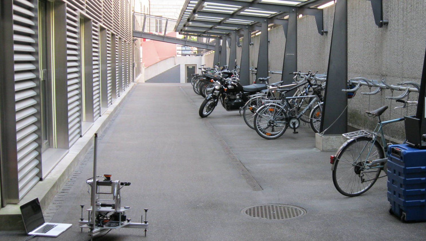
(a) Highly structured “stairs” (ST) environment

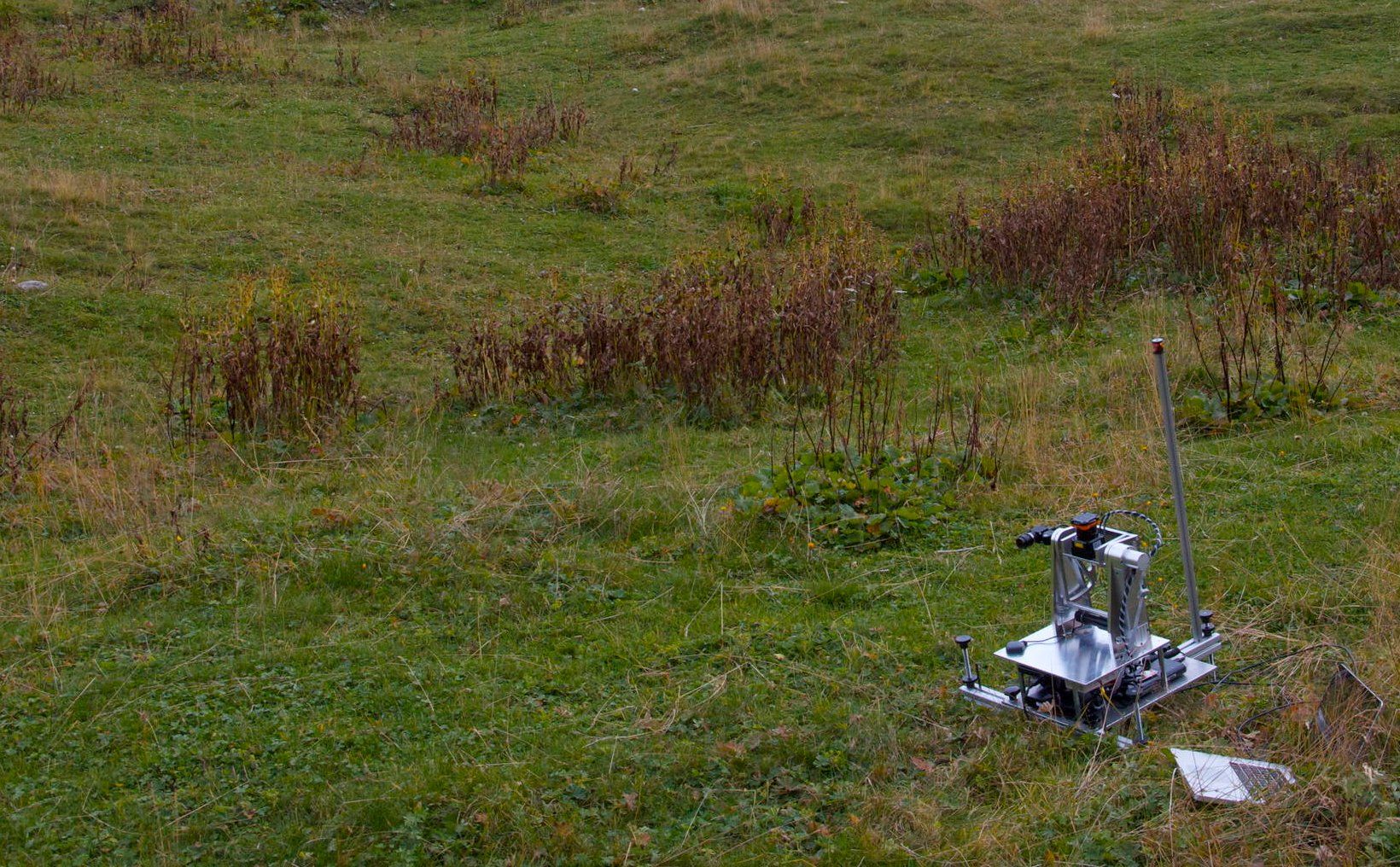
(b) Semi-structured “mountain plain” (MP)

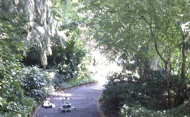
(c) Unstructured “wood in summer” (WS)

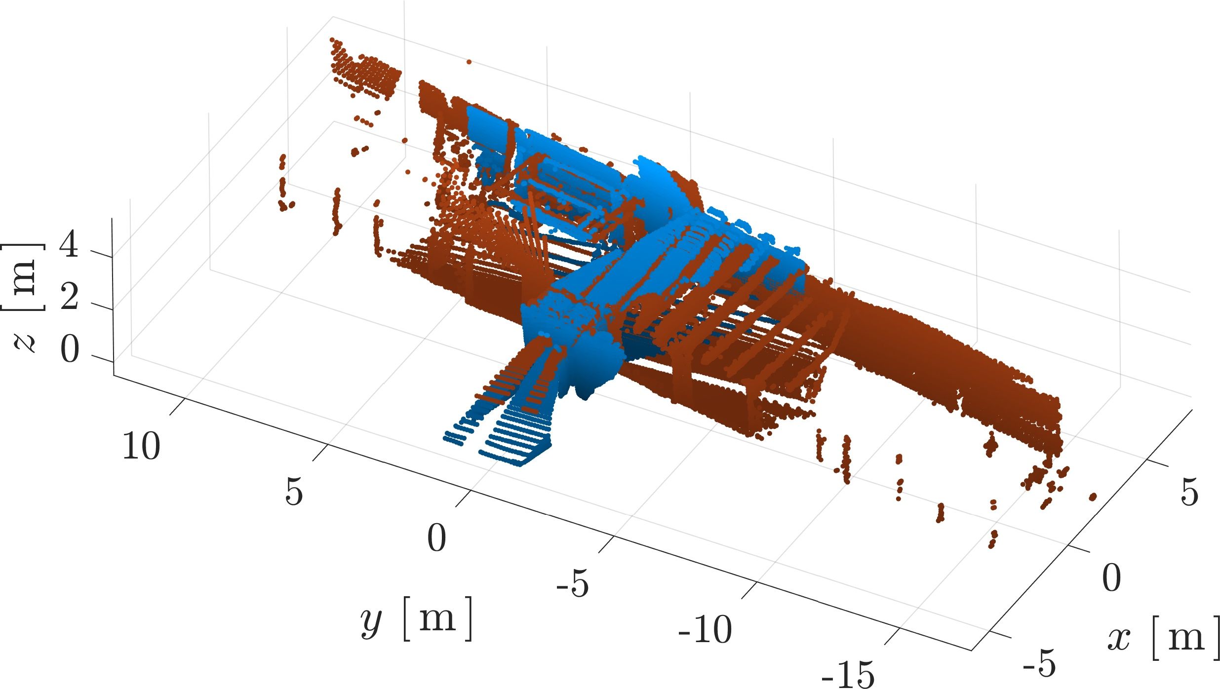
(d) Two scans from “stairs”

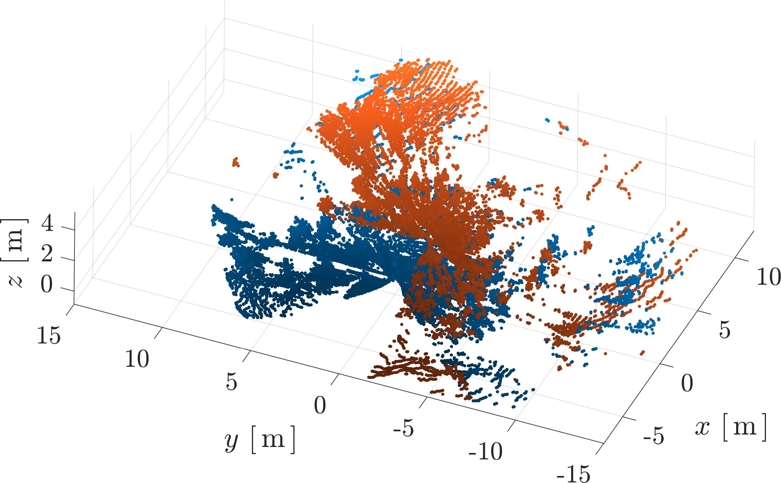
(e) Two scans from “mountain plain”

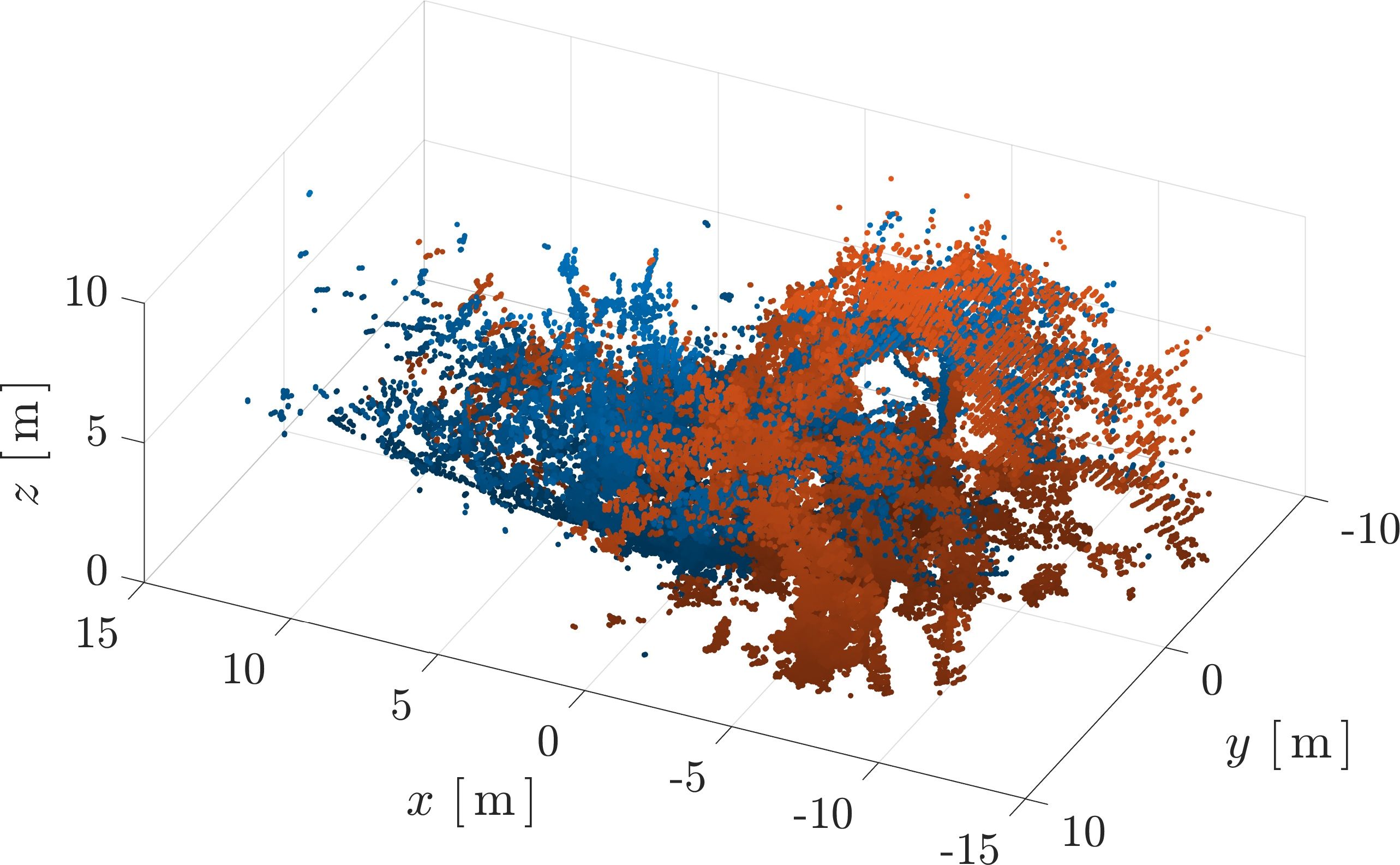
(f) Two scans from “wood in summer”

Figure 2: Contextual images and point cloud scans from the different environments studied [17]. The point cloud scans have been downsampled and the orange source cloud perturbed about it’s ground-truth pose relative to the blue target cloud.

To perform one trial, two scans from an environment are randomly assigned to $\mathcal{S}$ and $\mathcal{T}$. The scans are selected across trials to provide a uniform sampling of the overlap ratio between $40\text{\,}\mathrm{\char 37\relax}$ and $99\text{\,}\mathrm{\char 37\relax}$. ICP is then initialized according to ${\check{\mbf{T}}_{12}=\mbf{T}_{12}\delta\check{\mbf{T}}}$, where $\mbf{T}_{12}$ is the ground-truth pose of $\mathcal{S}$ relative to $\mathcal{T}$ and $\delta\check{\mbf{T}}(\delta\check{\mbf{C}}(\delta\check{\bm{\phi}}),\delta\check{\mbf{r}})$ is a random perturbation generated from

$$\delta\check{\bm{\phi}}\sim\mathcal{N}(\mbf{0},\sigma^{2}_{\phi}\mbf{1}),\quad\delta\check{\mbf{r}}\sim\mathcal{N}(\mbf{0},\sigma^{2}_{\textrm{r}}\mbf{1}).$$ (29)

Parameters $\sigma_{\phi}$ and $\sigma_{\textrm{r}}$ are set such that ${\|\delta\check{\bm{\phi}}\|<\phi_{\textrm{max.}}}$ and ${\|\delta\check{\mbf{r}}\|<r_{\textrm{max.}}}$ for $99.73\text{\,}\mathrm{\char 37\relax}$ of the trials. These limits are set to ${\phi_{\textrm{max.}}=$20\text{\,}\deg$}$ and ${r_{\textrm{max.}}=$0.5\text{\,}\mathrm{m}$}$, generally corresponding to a “medium” level of perturbation difficulty [18]. To accomodate the large residuals initially expected as the result of a poor prior relative pose estimate, the truncation bound is set to ${\tau=40}$ for all adaptive methods.

$\mathcal{S}$ is then aligned to $\mathcal{T}$ within an ICP framework using different RLFs. ICP settings are given in Table I, with subsampling performed in the sensor frame. Seven RLFs are included in this study. Cauchy [5], Tukey [19], and Welsch [7] loss functions implemented with median of absolute deviation (MAD) rescaling [20], as well as the Var. Trimmed loss function [21], are fixed functions included for their good performance in a similar study [22]. “Adaptive Barron” is the original adaptive function [8], and “Adaptive Chebrolu” is the recent modification [9]. These are compared to the proposed approach, called “Adaptive Maxwell-Boltzmann (MB).”

While a squared point-to-plane error is minimized by ICP, the residual ${\epsilon_{i}=\small\sqrt{\mathchoice{\mathsm@sh\displaystyle{\mbf{e}_{ij}^{\mathsf{T}}\bm{\Sigma}_{ij}^{-1}\mbf{e}_{ij}}}{\mathsm@sh\textstyle{\mbf{e}_{ij}^{\mathsf{T}}\bm{\Sigma}_{ij}^{-1}\mbf{e}_{ij}}}{\mathsm@sh\scriptstyle{\mbf{e}_{ij}^{\mathsf{T}}\bm{\Sigma}_{ij}^{-1}\mbf{e}_{ij}}}{\mathsm@sh\scriptscriptstyle{\mbf{e}_{ij}^{\mathsf{T}}\bm{\Sigma}_{ij}^{-1}\mbf{e}_{ij}}}}}$ used by all RLFs to perform outlier rejection is constructed using the point-to-point error,

$$\mbf{e}_{ij}= \ \mbf{r}^{p_{j}z_{1}}_{b_{1}}-\left(\mbf{r}^{z_{2}z_{1}}_{b_{1}}+\mbf{C}_{b_{1}b_{2}}\mbf{r}^{p_{i}z_{2}}_{b_{2}}\right),$$ (30a)

$$\bm{\Sigma}_{ij}= \ \mbf{C}_{b_{1}b_{2}}\mbf{R}_{i}\mbf{C}^{\mathsf{T}}_{b_{1}b_{2}}+\mbf{R}_{j},$$ (30b)

where ${\mbf{R}_{i},\mbf{R}_{j}}$ are the covariances on point measurements $\mbf{r}^{p_{i}z_{2}}_{b_{2}}$ and $\mbf{r}^{p_{j}z_{1}}_{b_{1}}$, respectively. To reduce the number of residual terms, $\mathcal{S}$ is subsampled on a $10\text{\,}\mathrm{cm}$ voxel grid. The covariance on the point measurements is set to ${\mbf{R}_{i}=\mbf{R}_{j}=\sigma_{\ell}^{2}\mbf{1}}$, with ${\sigma_{\ell}=$3\text{\,}\mathrm{cm}$}$, as reported in [17]. Posterior errors $\|\delta\hat{\bm{\phi}}\|$ and $\|\delta\hat{\bm{\rho}}\|$ corresponding to ICP posterior estimate $\hat{\mbf{T}}_{12}$ are reported according to (27), with ${\delta\hat{\mbf{T}}=\mbf{T}_{12}^{-1}\hat{\mbf{T}}_{12}}$. 180 trials per RLF were performed in each environment, with results in Table II.

TABLE I: Point cloud preprocessing and alignment parameters

Stage	Configuration	Description
Preprocessing	VoxelGrid	Subsample $\mathcal{S}$ on $10\text{\,}\mathrm{cm}$ grid
	Normals	From 15 nearest neighbours
ICP data assn.	KDTree	Single nearest neighbour
ICP error min.	Pt-pl	Point-to-plane error
Termination	Diff.	${\|\delta\bm{\phi}_{i}\|<$110-3\text{\,}\mathrm{rad}$\textrm{, and}}$ ${\|\delta\bm{\rho}_{i}\|<$110-3\text{\,}\mathrm{m}$}$
	Counter	50 iterations max

The proposed Adaptive MB approach delivers the lowest median rotation and translation errors across most experiments. However, what is especially notable about this approach is the large reduction in error variability, measured by the $75\text{\,}\mathrm{\char 37\relax}$ and $90\text{\,}\mathrm{\char 37\relax}$ error bounds for the adaptive RLFs on the right side of Table II. This reduction is more pronounced for less structured environments. For example, on the highly unstructured “wood in summer” (WS) dataset, $90\text{\,}\mathrm{\char 37\relax}$ of translation errors for Adaptive MB are below $5.2\text{\,}\mathrm{cm}$, compared with $7.2\text{\,}\mathrm{cm}$ for the original adaptive RLF [8] and $22.8\text{\,}\mathrm{cm}$ for the recent modification [9]. The reduction in variability is also evident for rotation errors, with $90\text{\,}\mathrm{\char 37\relax}$ of rotation errors in the WS dataset falling below $0.64\text{\,}\deg$ for Adaptive MB, compared with $1.09\text{\,}\deg$ for Adaptive Barron and $9.00\text{\,}\deg$ for Adaptive Chebrolu. This reduction in variability is clearly seen in the violin plots in Figure 3.

The bottom two rows of Table II give the median number of iterations to convergence and the median convergence time for all RLFs, taken across all datasets. Adaptive MB converges in fewer iterations than all the other methods surveyed and, despite the additional optimization step involved, converges in less time than the other adaptive methods. Note that this study was conducted using non-optimized MATLAB code, and timing results are included for relative comparison. On average, the fixed RLFs produced larger median errors and more severe failures than the adaptive RLFs, highlighting the effectiveness of adaptive methods.

Table III shows the success rate of each RLF for the different datasets. A trial is considered successful if the RLF is able to reduce both the rotation and translation error over the initial perturbation. With the exception of Var. Trimmed, the adaptive RLFs generally outperform the fixed RLFs across the different environments, however of all the methods surveyed the proposed Adaptive MB RLF has the highest success rate.

These improvements have been realized solely from a modification to the association weights $w_{ij}$ in (28). Adaptive MB is able to improve on existing methods because it avoids downweighting inliers, leading to lower median errors, lower variability, and fewer iterations to convergence.

TABLE II: ICP alignment errors and timing results for the environments studied using different RLFs. Results are also combined across environments (ALL). Median errors are reported for the four fixed RLFs, while cumulative statistics are reported for the adaptive RLFs in the format 50%-75%-90%, corresponding to the upper bounds of the error bars shown in Figure 3. The lowest median error in each row appears in bold font, as well as the lowest 75% and 90% errors for the adaptive RLFs. The median number of iterations and execution time are reported across all datasets for relative comparison.

Environment		Cauchy MAD	Tukey MAD	Welsch MAD	Var. Trimmed	Adaptive Barron [8]	Adaptive Chebrolu [9]	Adaptive MB (ours)
$\|\delta\hat{\bm{\phi}}\|$ $\left[\deg\right]$	ST	0.29	0.27	0.24	0.23	0.23-0.41-0.83	0.21-0.31-0.55	0.21-0.32-0.48
	MP	0.57	0.42	0.39	0.30	0.36-0.64-1.77	0.29-0.54-3.49	0.27-0.44-0.68
	WS	0.39	0.31	0.28	0.27	0.28-0.47-1.09	0.30-2.51-9.00	0.28-0.42-0.64
	ALL	0.41	0.31	0.29	0.26	0.29-0.48-1.11	0.26-0.46-5.79	0.26-0.40-0.61
$\|\delta\hat{\bm{\rho}}\|$ $\left[\operatorname{m}\!\operatorname{m}\right]$	ST	14	12	11	11	11-24-226	9-16-65	10-18-34
	MP	66	47	43	36	36-103-293	35-64-213	34-63-151
	WS	24	22	21	20	19-32-72	22-61-228	22-35-52
	ALL	29	26	24	23	22-43-217	21-46-205	22-39-79
Iterations	ALL	20	20	22	24	23	26	17
Time $\left[$\text{\,}\mathrm{s}$\right]$	ALL	2.75	2.75	2.94	3.38	3.64	4.21	2.83

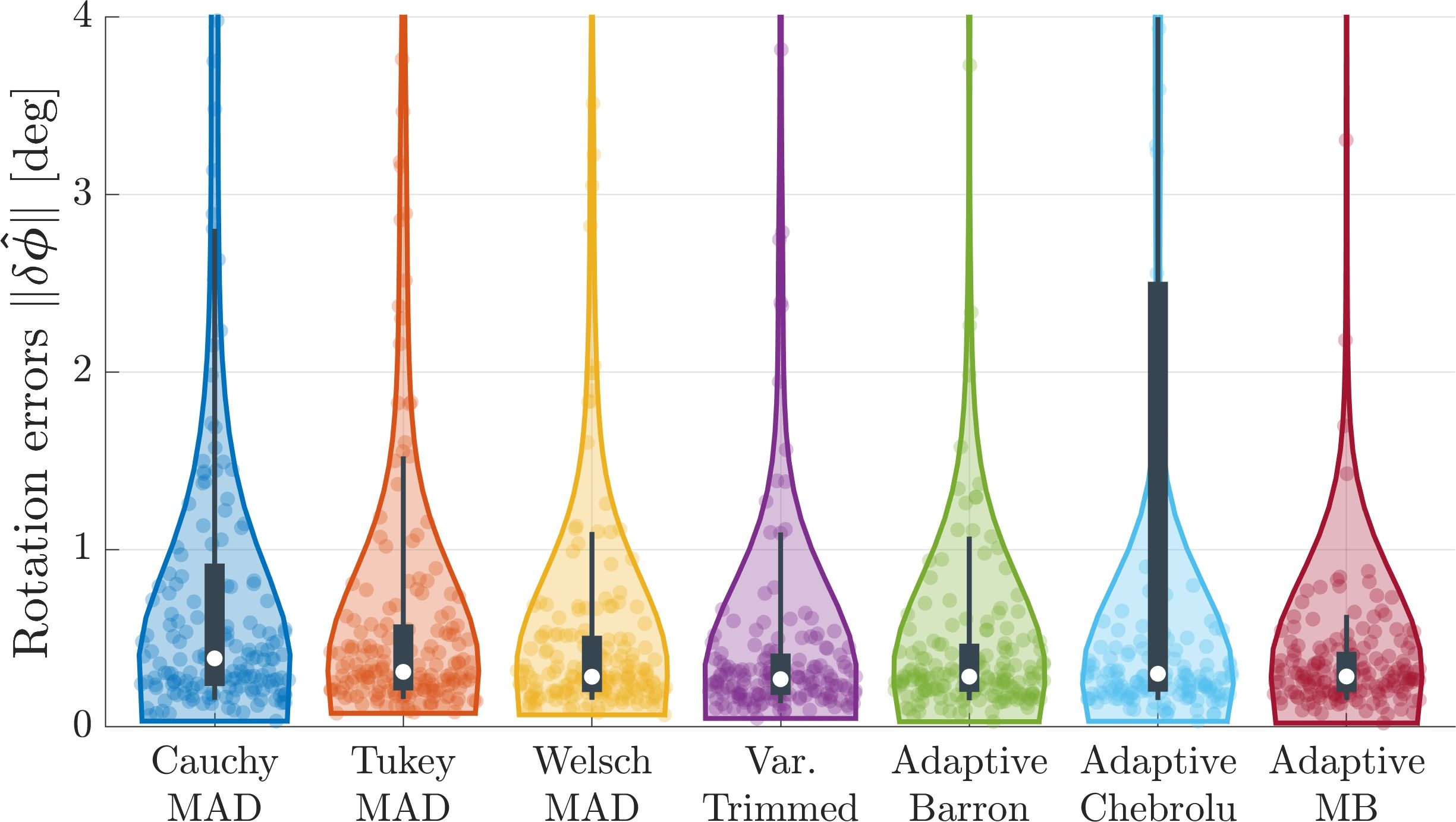
(a) Rotation errors, wood in summer (WS) dataset (180 trials)

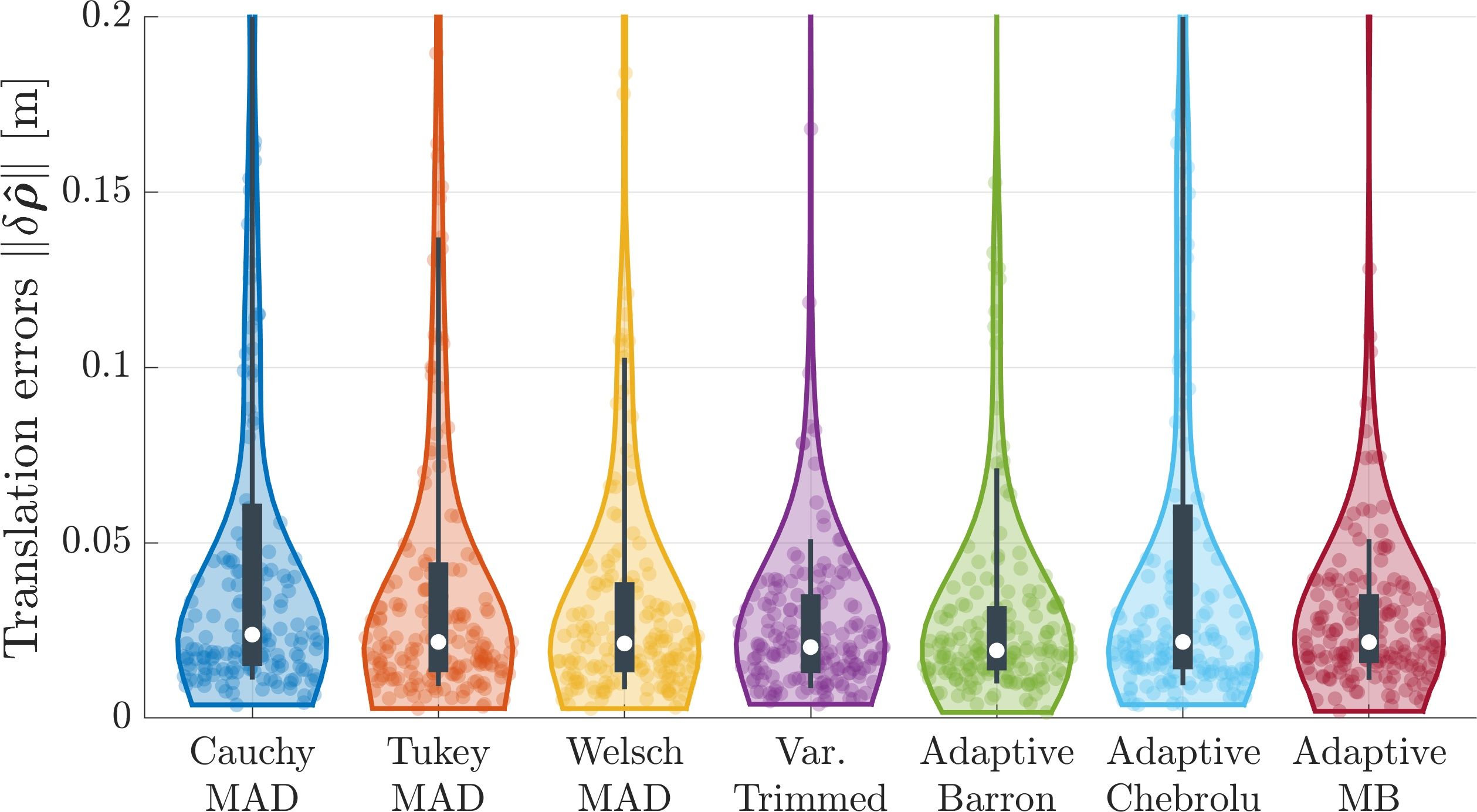
(b) Translation errors, WS dataset

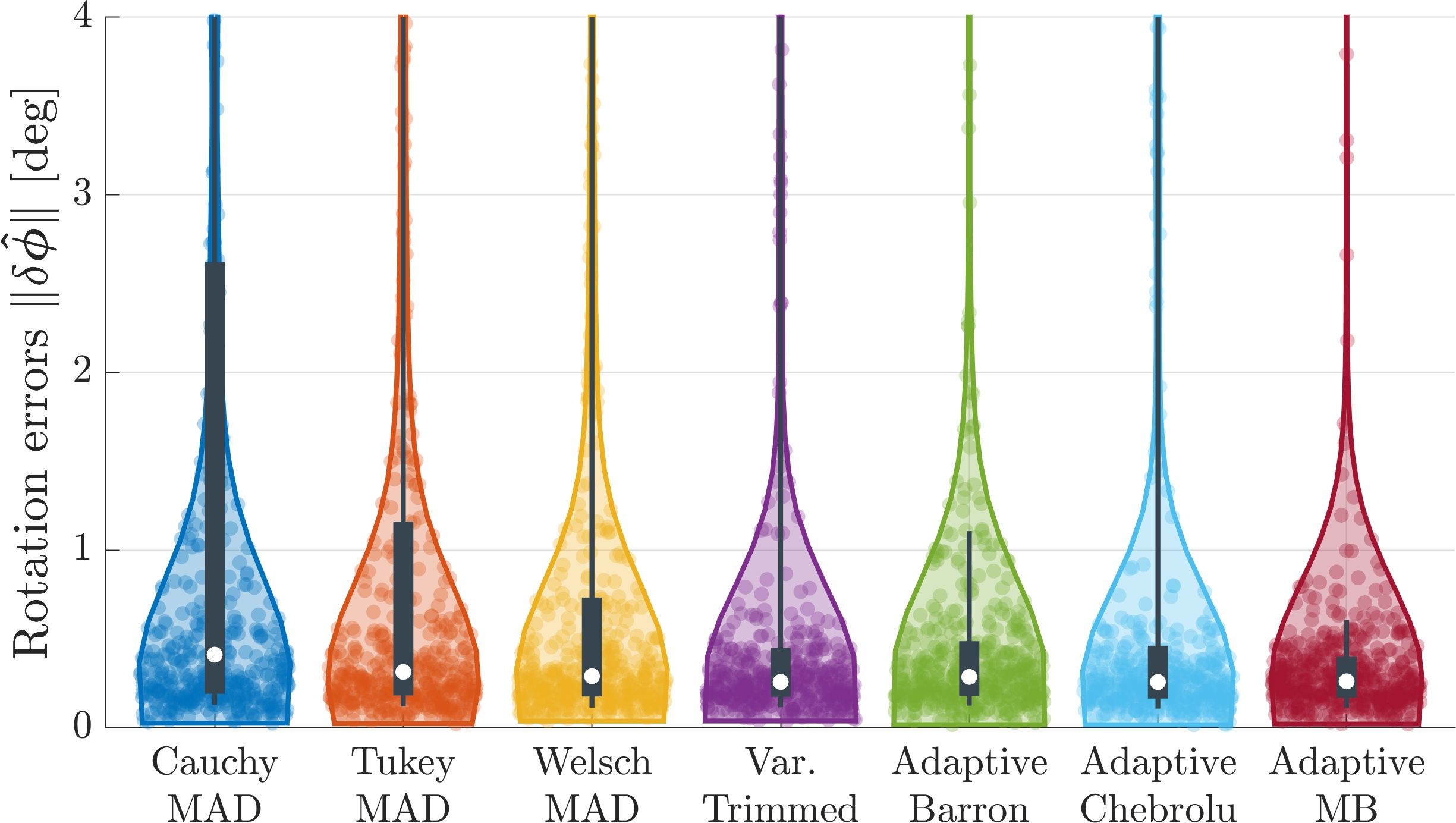
(c) Rotation errors, combined across datasets (ALL, 540 trials)

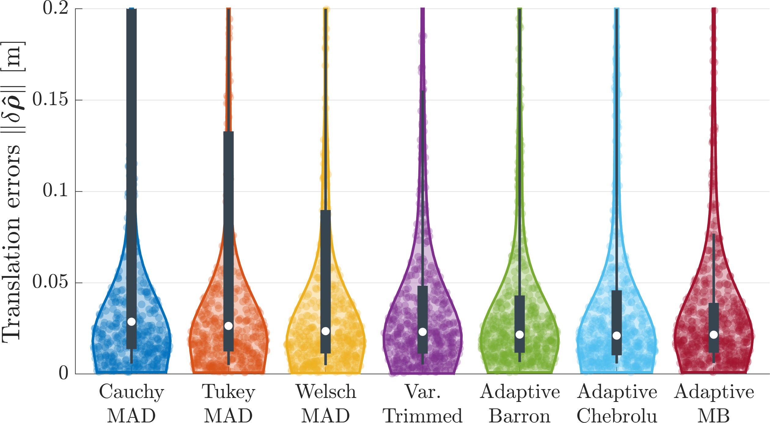
(d) Translation errors, combined across datasets

Figure 3: Violin plots showing the distribution of ICP alignment errors. Scatter plots show errors from individual trials, while envelopes show their relative frequency. Box plots show the middle $50\text{\,}\mathrm{\char 37\relax}$ (thick bar) and $80\text{\,}\mathrm{\char 37\relax}$ (thin bar) of the data, as well as the median (white dot). Median errors for Adaptive MB are slightly lower than state-of-the-art adaptive approaches across different environments, however the variability is markedly lower, especially for unstructured environments like WS (top row).

TABLE III: Comparing the percentage of successful alignments using different RLFs. An alignment is considered successful if it reduces both the rotation and translation error over the initial perturbation, ${\|\delta\hat{\bm{\phi}}\|<\|\delta\check{\bm{\phi}}\|}$ and ${\|\delta\hat{\bm{\rho}}\|<\|\delta\check{\bm{\rho}}\|}$.

RLF	ST	MP	WS	ALL
Cauchy-MAD	76.7%	53.9%	85.0%	71.9%
Tukey-MAD	78.9%	62.2%	91.1%	77.4%
Welsch-MAD	79.4%	68.3%	93.9%	80.6%
Var. Trimmed	87.8%	90.0%	96.7%	91.5%
Adaptive Barron [8]	88.3%	85.6%	96.1%	90.0%
Adaptive Chebrolu [9]	92.8%	88.9%	88.3%	90.0%
Adaptive MB (ours)	96.1%	92.2%	98.3%	95.6%

IV-C Pose Averaging

Pose averaging is a second fundamental state estimation problem, often encountered in camera-based applications such as structure from motion (SfM) [23]. A pose averaging study was performed investigating the effectiveness of the RLFs in a six degree-of-freedom problem with high outlier rates.

Given a set of pose measurements $\{\tilde{\mbf{T}}_{i}\}\vphantom{\{\mbf{T}_{i}\}}^{N}_{i=1}$ with associated covariances $\left\{\mbf{R}\right\}\!\vphantom{\left\{\mbf{R}\right\}}^{N}_{i=1}$, ${\mbf{R}_{i}=\mathrm{E}[\delta\tilde{\bm{\xi}}_{i}\,\delta\tilde{\bm{\xi}}^{\mathsf{T}}_{i}]}$, pose averaging returns the optimal average pose,

$$\mbf{T}^{\star}=\operatorname*{arg\,min}_{\mbf{T}\in SE(3)}\frac{1}{2}\sum^{N}_{i=1}w_{i}\cdot\left\|\mbf{e}_{i}(\mbf{T},\tilde{\mbf{T}}_{i})\right\|^{2}_{\bm{\Sigma}^{-1}_{i}},\vspace{6pt}$$ (31)

with left-invariant pose error ${\mbf{e}_{i}=\log\left(\mbf{T}^{-1}\,\tilde{\mbf{T}}_{i}\right)^{\vee}}$ [16, §5.2.1]. Perturbing to first order yields the batch Jacobians,

$$\delta\mbf{e}_{i}=\underbrace{\mbf{J}^{\ell}(\bar{\mbf{e}}_{i})^{-1}}_{\mbf{H}_{i}}\delta\bm{\xi}_{i}\underbrace{-\mbf{J}^{\textrm{r}}(\bar{\mbf{e}}_{i})^{-1}}_{\mbf{M}_{i}}\delta\tilde{\bm{\xi}}_{i},\vspace{6pt}$$ (32)

where $\mbf{J}^{\ell},\mbf{J}^{\textrm{r}}$ are, respectively, the left and right Jacobians of $SE(3)$ [12, §7.1.5]. The covariance on the pose errors is then ${\bm{\Sigma}_{i}=\mbf{M}_{i}\mbf{R}_{i}\mbf{M}^{\mathsf{T}}_{i}}$. The residual $\epsilon_{i}$ is defined via (14). If $\mbf{e}_{i}$ is normally distributed, then $\epsilon_{i}$ will follow a Chi distribution with six degrees of freedom, with a mode of ${\tilde{\epsilon}=\sqrt{5}}$ [13, §11.3]. By accounting for this gap, Adaptive MB is expected to converge faster with better overall performance than existing RLFs.

A simulated Monte Carlo experiment was performed in which a pose averaging problem was corrupted by an increasing number of outliers. For all trials, 20 inlier measurements were randomly generated according to ${\tilde{\mbf{T}}^{\textrm{in}}_{i}=\exp(\delta\tilde{\bm{\xi}}_{i}^{\wedge})}$, with ${\delta\tilde{\bm{\xi}}_{i}\sim\mathcal{N}(\mbf{0},\mbf{R})}$. Outlier measurements were generated uniformly according to ${\mbf{T}^{\textrm{out}}_{i}(\mbf{C}_{i}(\bm{\phi}_{i}^{\textrm{out}}),\mbf{r}_{i}^{\textrm{out}})}$, where ${\bm{\phi}^{\textrm{out}}_{i}\in\left[-$60\text{\,}\deg$,$60\text{\,}\deg$\right]}$ and ${\mbf{r}^{\textrm{out}}_{i}\in\left[-\color[rgb]{0,0,0}{$2.5\text{\,}\mathrm{m}$}\color[rgb]{0,0,0},\color[rgb]{0,0,0}{$2.5\text{\,}\mathrm{m}$}\color[rgb]{0,0,0}\right]}$. The proportion of outlier measurements was increased from $20\text{\,}\mathrm{\char 37\relax}$ to $80\text{\,}\mathrm{\char 37\relax}$ in $20\text{\,}\mathrm{\char 37\relax}$ increments. 100 trials were run at each outlier level, with $\check{\mbf{T}}$ initialized according to ${\check{\mbf{T}}=\exp(\delta\check{\bm{\xi}}^{\wedge})}$, ${\delta\check{\bm{\xi}}\sim\mathcal{N}(\mbf{0},\check{\mbf{P}})}$. A trial converged when the update fell below the thresholds ${\|\delta\bm{\phi}_{i}\|<$110-3\text{\,}\mathrm{rad}$}$ and ${\|\delta\bm{\rho}_{i}\|<$110-3\text{\,}\mathrm{m}$}$. Trials were terminated after 50 iterations. Figure 4 shows the setup for a single trial, including a visualization of $\mbf{R}$ and $\check{\mbf{P}}$. The truncation bound $\tau$ was set to 40 for all adaptive approaches. The pose averaging experiment is intentionally simple, to evaluate the behaviour of the different RLFs under tightly controlled conditions.

The results are summarized in Table IV. Adaptive Chebrolu [9] performs reasonably well at low outlier levels, but becomes increasingly conservative ${(\alpha^{\star}\to-\infty)}$ as the proportion of outliers is increased, resembling Welsch loss. The effect on the optimization is twofold. First, the (low) weights assigned to the inlier residuals clustered around the mode at ${\tilde{\epsilon}=\sqrt{5}}$ become increasingly indistinguishable from the weights assigned to the outlier residuals. Second, the number of outlier terms grows relative to the number of inlier terms. These effects combine to yield reduced performance at higher outlier levels.

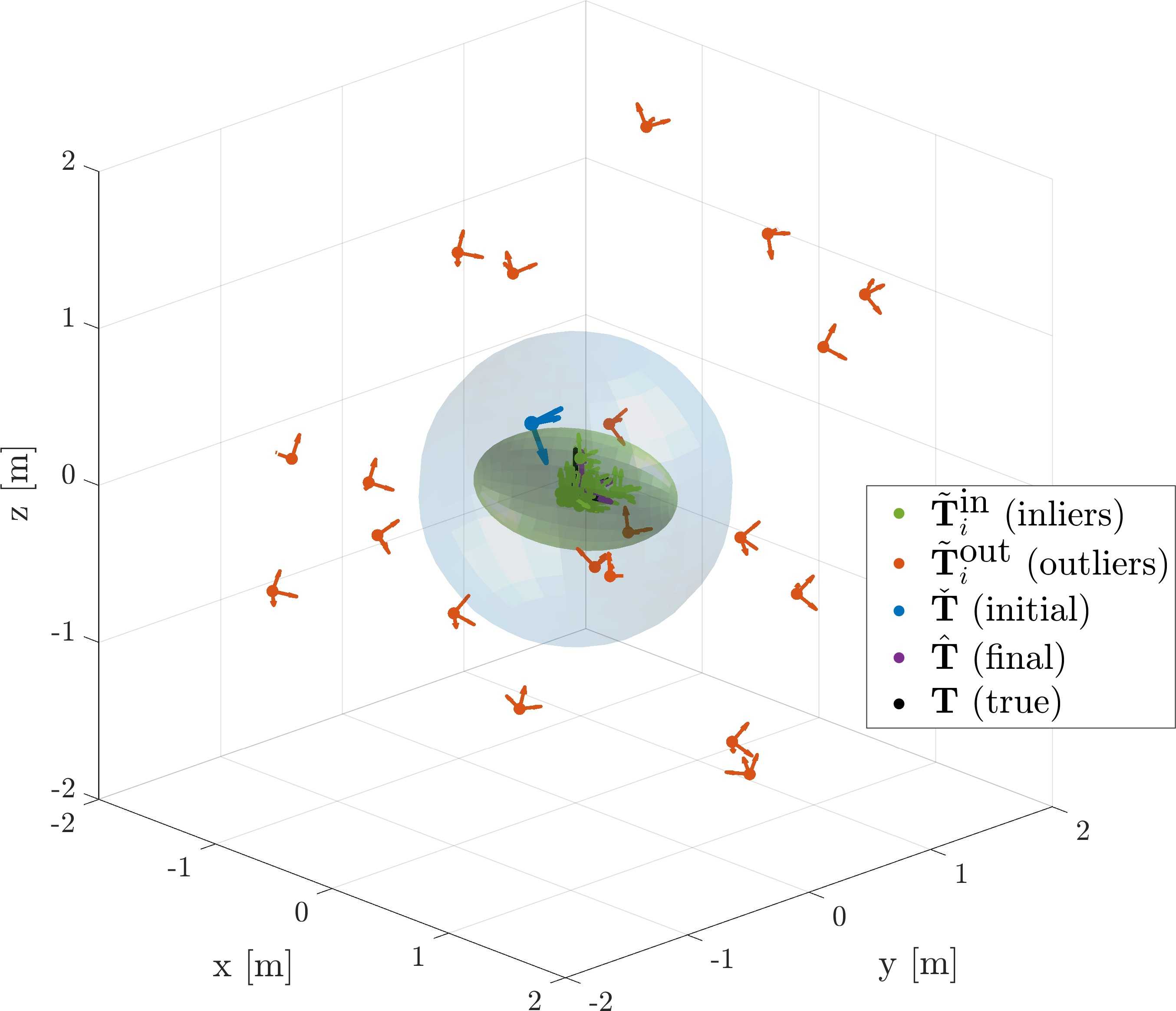
Figure 4: A pose averaging trial with a $60\text{\,}\mathrm{\char 37\relax}$ outlier rate. The green and blue ellipsoids are the $99.73\text{\,}\mathrm{\char 37\relax}$ confidence bounds on $\mbf{R}$ and $\check{\mbf{P}}$, respectively. Note $\mbf{R}$ is non-isotropic, highlighting the importance of using the Mahalanobis distance as the residual.

The original Adaptive Barron [8] approach generally avoids this, as the shape parameter is bounded from below by zero, resembling Cauchy loss. The optimization is better able to differentiate inliers from outliers by the relative magnitude of their association weight, leading to reasonable performance. However, the weights assigned to the inliers are still low, leading to slower convergence.

In contrast, Adaptive MB acknowledges the “mode gap,” assigning an association weight of ${w_{i}=1}$ to inlier residuals ${\epsilon_{i}<\tilde{\epsilon}}$. This approach converges more quickly than the other adaptive methods, with a median execution time of $0.13\text{\,}\mathrm{s}$. In nearly all trials, accounting for the underlying distribution on $\epsilon_{i}$ produces the lowest median error, with a marked decrease in error variability compared to other adaptive methods.

Notably, Var. Trimmed also yields excellent median performance across all pose averaging trials, with a much lower median execution time than Adaptive MB. This truncated loss function may therefore prove a useful alternative for time-sensitive applications.

TABLE IV: Pose errors and timing results from the simulated pose averaging experiment, showing either median values or a 50%-75%-90% distribution. As the proportion of outliers goes up, Adaptive Chebrolu [9] grows increasingly conservative ($\alpha^{\star}\to-\infty$), resembling Welsch loss. However, because the mode of the residuals occurs at ${\tilde{\epsilon}>0}$, both inliers and outliers are assigned an approximately equal (low) weight, yielding poorer performance. Adaptive Barron [8] generally avoids this, as $\alpha$ is bounded from below by zero, resembling Cauchy loss. Adaptive MB converges faster than the other adaptive methods, both in terms of iterations and execution time, because inliers ${\epsilon_{i}<\tilde{\epsilon}}$ are highly weighted.

Percent outliers		Cauchy MAD	Tukey MAD	Welsch MAD	Var. Trimmed	Adaptive Barron [8]	Adaptive Chebrolu [9]	Adaptive MB (ours)
$\|\delta\hat{\bm{\phi}}\|$ $\left[\deg\right]$	$20\text{\,}\mathrm{\char 37\relax}$	1.92	1.78	5.22	1.72	1.81-2.36-2.91	1.90-2.39-3.00	1.64-2.23-2.95
	$40\text{\,}\mathrm{\char 37\relax}$	1.80	1.72	2.15	1.76	1.86-2.40-3.09	1.91-2.52-3.27	1.68-2.25-2.84
	$60\text{\,}\mathrm{\char 37\relax}$	9.29	12.51	6.20	1.65	1.74-2.32-3.07	1.99-2.58-3.28	1.60-2.23-2.83
	$80\text{\,}\mathrm{\char 37\relax}$	5.88	8.89	2.42	1.95	2.11-2.67-3.28	2.88-3.83-4.96	1.78-2.32-2.84
$\|\delta\hat{\bm{\rho}}\|$ $\left[\operatorname{m}\!\operatorname{m}\right]$	$20\text{\,}\mathrm{\char 37\relax}$	43	41	106	42	42-64-77	42-67-77	42-61-78
	$40\text{\,}\mathrm{\char 37\relax}$	38	37	47	35	38-66-84	43-65-87	38-61-80
	$60\text{\,}\mathrm{\char 37\relax}$	210	344	155	39	40-61-69	45-65-78	39-53-64
	$80\text{\,}\mathrm{\char 37\relax}$	139	277	52	39	46-62-80	67-105-131	36-50-64
Time $\left[$\text{\,}\mathrm{s}$\right]$	ALL	0.04	0.04	0.04	0.02	0.18-0.21-0.23	0.22-0.27-0.37	0.13-0.15-0.17
Iterations	ALL	7.0	8.0	7.0	3.0	6.0-7.0-7.0	8.0-9.0-12.0	4.0-5.0-5.0

V Conclusion

Outlier rejection is a key component of real-world robotics problems. Many problems in robotics involve least-squares optimization, where the residual is the norm of some multivariate, normally distributed error. The residual will then follow a Chi distribution, with a mode value of ${\tilde{\epsilon}>0}$. Existing RLFs assume a mode of zero, leading to the creation of a “mode gap” that impacts convergence times and optimization accuracy. By accounting for this gap, the proposed “Adaptive MB” approach is able to deliver faster convergence times and more robust performance than existing adaptive RLFs [8, 9], as well as the fixed RLFs studied. This was demonstrated for two fundamental state estimation problems, point cloud alignment and pose averaging. The results suggest this approach will be widely applicable to least-squares optimization problems in state estimation and robotics.

References

- [1] Paul F. Roysdon and Jay A. Farrell “GPS-INS outlier detection & elimination using a sliding window filter” In Amer. Control Conf. (ACC), 2017, pp. 1244–1249 IEEE
- [2] José Neira and Juan D Tardós “Data association in stochastic mapping using the joint compatibility test” In IEEE Trans. Robot. Automat. 17.6 IEEE, 2001, pp. 890–897
- [3] Peter J Huber “Robust estimation of a location parameter” In The Annals of Mathematical Statistics 35.1 Springer, 1964, pp. 73–101
- [4] Zhengyou Zhang “Parameter estimation techniques: A tutorial with application to conic fitting” In Image Vis. Comput. 15.1 Elsevier, 1997, pp. 59–76
- [5] Michael J. Black and Paul Anandan “The robust estimation of multiple motions: Parametric and piecewise-smooth flow fields” In Comput. Vis. Image Understanding 63.1 Elsevier, 1996, pp. 75–104
- [6] Stuart Geman and Donald E. McClure “Bayesian image analysis: An application to single photon emission tomography” In Proc. Amer. Stat. Assoc., 1985, pp. 12–18
- [7] John E. Dennis Jr. and Roy E. Welsch “Techniques for nonlinear least squares and robust regression” In Commun. Stat. - Simul. Comput. 7.4 Taylor & Francis, 1978, pp. 345–359
- [8] Jonathan T Barron “A general and adaptive robust loss function” In Proc. IEEE Conf. Comput. Vis. Pattern Recognit., 2019, pp. 4331–4339
- [9] Nived Chebrolu et al. “Adaptive robust kernels for non-linear least squares problems” In IEEE Robot. Auton. Lett. (RAL) 6.2 IEEE, 2021, pp. 2240–2247
- [10] DQF De Menezes, Diego M Prata, Argimiro R Secchi and José Carlos Pinto “A review on robust M-estimators for regression analysis” In Comput. & Chem. Eng. 147 Elsevier, 2021, pp. 107254
- [11] Rick Chartrand and Wotao Yin “Iteratively reweighted algorithms for compressive sensing” In IEEE Int. Conf. Acoust., Speech, Signal Process., 2008, pp. 3869–3872
- [12] Timothy D Barfoot “State Estimation for Robotics” Cambridge University Press, 2017
- [13] Catherine Forbes, Merran Evans, Nicholas Hastings and Brian Peacock “Statist. Distributions” John Wiley & Sons, 2010
- [14] Normand M. Laurendeau “Statist. Thermodynamics: Fundam. Appl.” Cambridge University Press, 2005 DOI: 10.1017/CBO9780511815928
- [15] Joan Sola, Jeremie Deray and Dinesh Atchuthan “A micro Lie theory for state estimation in robotics” In arXiv preprint arXiv:1812.01537, 2018
- [16] Jonathan Arsenault “Practical Considerations and Extensions of the Invariant Extended Kalman Filtering Framework”, 2019
- [17] François Pomerleau, Ming Liu, Francis Colas and Roland Siegwart “Challenging data sets for point cloud registration algorithms” In Int. J. Robot. Res. 31.14 SAGE Publications Sage UK: London, England, 2012, pp. 1705–1711
- [18] François Pomerleau, Francis Colas, Roland Siegwart and Stéphane Magnenat “Comparing ICP variants on real-world data sets: Open-source library and experimental protocol” In Auton. Robots 34.3 Springer, 2013, pp. 133–148
- [19] Albert E. Beaton and John W. Tukey “The fitting of power series, meaning polynomials, illustrated on band-spectroscopic data” In Technometrics 16.2 Taylor & Francis, 1974, pp. 147–185
- [20] Robert M Haralick et al. “Pose estimation from corresponding point data” In IEEE Trans. Syst., Man, Cybern. 19.6 IEEE, 1989, pp. 1426–1446
- [21] Jeff M Phillips, Ran Liu and Carlo Tomasi “Outlier robust ICP for minimizing fractional RMSD” In Int. Conf. 3D Digit. Imag. Model. (3DIM), 2007, pp. 427–434 IEEE
- [22] Philippe Babin, Philippe Giguère and François Pomerleau “Analysis of Robust Functions for Registration Algorithms” In Proc. IEEE Int. Conf. Robot. Auton. (ICRA), 2019, pp. 1451–1457
- [23] Arman Karimian, Ziqi Yang and Roberto Tron “Rotational outlier identification in pose graphs using dual decomposition” In Eur. Conf. Comput. Vis. (ECCV), 2020, pp. 391–407 Springer