An Invertible Graph Diffusion Neural Network for Source Localization

Abstract.

Localizing the source of graph diffusion phenomena, such as misinformation propagation, is an important yet extremely challenging task in the real world. Existing source localization models typically are heavily dependent on the hand-crafted rules and only tailored for certain domain-specific applications. Unfortunately, a large portion of the graph diffusion process for many applications is still unknown to human beings so it is important to have expressive models for learning such underlying rules automatically. Recently, there is a surge of research body on expressive models such as Graph Neural Networks (GNNs) for automatically learning the underlying graph diffusion. However, source localization is instead the inverse of graph diffusion, which is a typical inverse problem in graphs that is well-known to be ill-posed because there can be multiple solutions and hence different from the traditional (semi-)supervised learning settings. This paper aims to establish a generic framework of invertible graph diffusion models for source localization on graphs, namely Invertible Validity-aware Graph Diffusion (IVGD), to handle major challenges including 1) Difficulty to leverage knowledge in graph diffusion models for modeling their inverse processes in an end-to-end fashion, 2) Difficulty to ensure the validity of the inferred sources, and 3) Efficiency and scalability in source inference. Specifically, first, to inversely infer sources of graph diffusion, we propose a graph residual scenario to make existing graph diffusion models invertible with theoretical guarantees; second, we develop a novel error compensation mechanism that learns to offset the errors of the inferred sources. Finally, to ensure the validity of the inferred sources, a new set of validity-aware layers have been devised to project inferred sources to feasible regions by flexibly encoding constraints with unrolled optimization techniques. A linearization technique is proposed to strengthen the efficiency of our proposed layers. The convergence of the proposed IVGD is proven theoretically. Extensive experiments on nine real-world datasets demonstrate that our proposed IVGD outperforms state-of-the-art comparison methods significantly. We have released our code at https://github.com/xianggebenben/IVGD.

1. Introduction

Graphs are prevalent data structures where nodes are connected by their relations. They have been widely applied in various domains such as social networks (scott1988social, ), biological networks (junker2011analysis, ), and information networks (harvey2006capacity, ). As a fundamental task in graph mining, graph diffusion aims to predict future graph cascade patterns given source nodes. However, its inverse problem, graph source localization, is rarely explored and yet is an extremely important topic. It aims to detect source nodes given their future graph cascade patterns. As an example shown in Figure 1, the goal of graph diffusion is to predict the cascade pattern $\{b,c,d,e\}$ given a source node $b$; while the goal of graph source localization is to detect source nodes $b$ or $c$ given the cascade pattern $\{b,c,d,e\}$. Graph source localization covers a wide range of promising research and real-world applications. For example, misinformation such as “drinking bleach or alcohol can prevent or kill the virus” (islam2020covid, ) in social networks is required to detect as early as possible, in order to prevent it from spreading; Email is a primary vehicle to transmit computer viruses, and thus tracking the source Emails carrying viruses in the Email networks is integral to computer security (newman2002email, ); malware detection aims to position the source of malware in the Internet of Things (IoT) network (jang2014mal, ). Therefore, the graph source localization problem entails attention and extensive investigations from machine learning researchers.
The forward process in Figure 1, namely, graph diffusion, has been studied for a long time, by traditional prescribed methods based on hand-crafted rules and heuristics such as SEHP (bao2015modeling, ), OSLOR (cui2013cascading, ), and DSHP (ding2015video, ). Following similar styles of traditional graph diffusion methods, classical methods for its inverse process, namely source localization of graph diffusion, have also been dominated by prescribed approaches. Specifically, a majority of methods are based on predefined rules, by utilizing either heuristics or metrics to select sources such as distance errors. Some other prescribed methods partition nodes into different clusters based on network topologies, and select source nodes in each cluster. These prescribed methods rely heavily on human predefined heuristics and rules and usually are specialized for specific applications. Therefore, they may not be suitable for applications where prior knowledge on diffusion mechanisms is unavailable. Recently, with the development of GNNs (GNNBook2022, ), Dong et al. utilized state-of-the-art architectures such as Graph Convolutional Network (GCN) to localize the source of misinformation (dong2019multiple, ). However, their method requires results from prescribed methods as its input, and hence still suffers from the drawback of prescribed methods mentioned above.

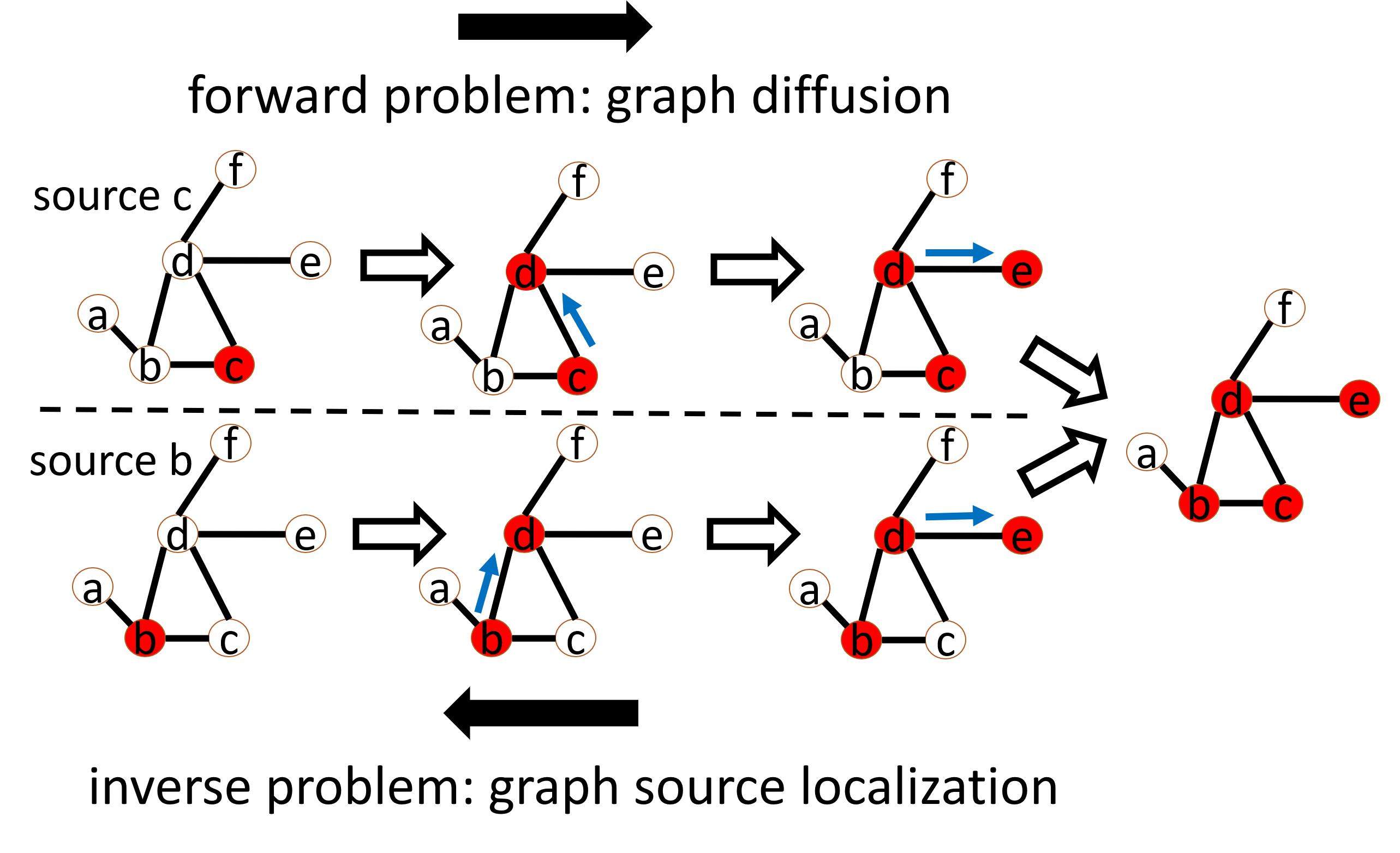
Figure 1. An example of information diffusion: different source nodes generate the same cascade pattern.

In recent years, the advancement of GNNs leads to state-of-the-art performance in many graph mining tasks such as node classification and link prediction. They can incorporate node attributes into models and learn node representations effectively by capturing network topology and neighboring information (kipf2016semi, ). They have recently expanded their success into graph diffusion problems (cao2020popularity, ), by tackling the drawbacks of traditional prescribed methods in graph diffusion. specifically, instead of requiring prior knowledge and rules of diffusion, GNNs based methods can ”learn” rules from the data in an end-to-end fashion. Although GNNs have been well applied for performing graph diffusion tasks, however, it is difficult to devise their inverse counterparts (i.e. graph source localization models) because such an inverse problem is much more difficult and involves three key challenges: 1). Difficulty to leverage knowledge in graph diffusion models for modeling their inverse processes in an end-to-end fashion. The learned knowledge from graph diffusion models facilitates source localization. For example, as shown in Figure 1, while nodes $b$ and $c$ generate the same cascade pattern $\{b,c,d,e\}$, the learned knowledge from graph diffusion models is useful to predict which node is likely to be the source. However, it is extremely challenging to incorporate such a notion into the inverse problem in an end-to-end manner, and it is prohibitively difficult to define hand-crafted ways to achieve it with graph diffusion models directly since they are opposite processes. 2). Difficulty to ensure the validity of the inferred sources. Graph sources usually follow validate graph patterns. For example, in the application of misinformation detection, sources of misinformation should be connected in the social networks. As another example, sources of malware are dense in some restricted regions of the IoT networks. Such validity constraints are imposed both in the training and test phases, which should be achieved by delicately-designed activation layers. Traditional activation layers such as softmax are exerted on individual nodes. However, validity constraints require the projection of multiple sources by considering their topological connections. 3). Efficiency and scalability in source inference. Inferring sources constrained by validity patterns is a combinatorial problem and hence is time-consuming. To multiply the difficulty, the inverse process of graph diffusion models should also be inferred. Therefore, devising a scalable and efficient algorithm is important yet challenging.
In this paper, we propose a novel Invertible Validity-aware Graph Diffusion (IVGD) to simultaneously tackle all these challenges. Specifically, given a graph diffusion model, we make it invertible by restricting its Lipschitz constant for the residual GNNs, and thus an approximate estimation of source localization can be obtained by its inversion, and then a compensation module is presented to reduce the introduced errors with skip connection. Moreover, we leverage the unrolled optimization technique to integrate validity constraints into the model, where each layer is encoded by a constrained optimization problem. To combat efficiency and scalability problems, a linearization technique is used to transform problems into solvable ones, which can be efficiently solved by closed-form solutions. Finally, the convergence of the proposed IVGD to a feasible solution is proven theoretically. Our contributions in this work can be summarized as follows:

• Design a generic end-to-end framework for source location. We develop a framework for the inverse of graph diffusion models, and learn rules of graph diffusion models automatically. It does not require hand-crafted rules and can be used for source localization. Our framework is generic to any graph diffusion model, and the code has been released publicly.

• Develop an invertible graph diffusion model with an error compensation mechanism. We propose a new graph residual net with Lipschitz regularization to ensure the invertibility of graph diffusion models. Furthermore, we propose an error compensation mechanism to offset the errors inferred from the graph residual net.

• Propose an efficient validity-aware layer to maintain the validity of inferred sources. Our model can ensure the validity of inferred sources by automatically learning validity-aware layers. We further accelerate the optimization of the proposed layers by leveraging a linearization technique. It transforms nonconvex problems into convex problems, which have closed-form solutions. Moreover, we provide the convergence guarantees of the proposed IVGD to a feasible solution.

• Conduct extensive experiments on nine datasets. Extensive experiments on nine datasets have been conducted to demonstrate the effectiveness and robustness of our proposed IVGD. Our proposed IVGD outperforms all comparison methods significantly on five metrics, especially $20\%$ on F1-Score.

2. Related Work

In this work, we summarize existing works related to this paper, which are shown as follows:
Graph Diffusion: Graph diffusion is the task of predicting the diffusion of information dissemination in networks. It has a wide range of real-world applications such as societal event prediction (wang2018incomplete, ; zhao2021event, ; zhao2017spatial, ), and adverse event detection in social media (wang2018multi, ; wang2018semi, ). A large number of research works have been conducted to improve the quality of predictions. Most existing works usually assume the topologies of networks and apply the classical probabilistic graphical models. For example, Ahmed et al. identified patterns of temporal evolution that are generalizable to distinct types of data (ahmed2013peek, ); Bandari et al. constructed a multi-dimensional feature space derived from properties of an article and evaluate the efficacy of these features to serve as predictors of online diffusion (bao2015modeling, ). More traditional methods can be found in various survey papers (moniz2019review, ; gao2019taxonomy, ; zhou2021survey, ). However, they are applicable to a specific type of neural network and are poorly generalizable. A recent line of research works use Recurrent Neural Networks (RNN) to predict the diffusion, and usually include multimodality such as text content and time series (bielski2018understanding, ; chen2019npp, ; chu2018cease, ; xie2020multimodal, ; zhang2018user, ). Various techniques have been applied including self-attention mechanism (bielski2018understanding, ; chen2017attention, ; wang2017cascade, ), knowledge base (zhao2019neural, ), multi-task learning (chen2019information, ), and stochastic processes (cao2017deephawkes, ; du2016recurrent, ; liao2019popularity, ) . However, they cannot utilize network topology to enhance predictions. To handle this challenge, GNNs have been applied to predict either macro-level (i.e. global level) tasks (cao2020popularity, ) or micro-level (i.e. node level) tasks (he2020network, ; qiu2018deepinf, ; wang2017topological, ; xia2021DeepIS, ) combined with RNN, and a handful of works attempted to utilize other neural network architectures (kefato2018cas2vec, ; sanjo2017recipe, ; wang2018factorization, ; yang2019neural, ).
Graph Source Localization: The goal of the graph source localization is to identify the source of a network based on observations such as the states of the nodes and a subset of timestamps at which the diffusion process reached the corresponding nodes (ying2018diffusion, ). Graph source localization has a wide range of applications such as disease localization, virus localization, and rumor detection. Several recent surveys on this topic are available (shah2010detecting, ; jiang2016identifying, ; shelke2019source, ). Similar to graph diffusion models, existing graph source localization papers usually require the assumptions of the diffusion, network topology, and observations. With the development of GNNs, Dong et al. proposed a Graph Convolutional Networks based Source Identification (GCNSI) model for multiple source localization (dong2019multiple, ). However, its model relies heavily on hand-crafted rules. Moreover, its performance suffers from the class imbalance problem, as shown in experiments.

Notations	Descriptions
$V$	Node set
$E$	Edge set
$Y_{t}$	Diffusion vector at time $t$
$x$	The vector of source nodes
$f_{W}$	The function of feature construction
$g$	The function of label propagation
$\Phi(x)=0$	The equality constraint of a validity pattern
$T$	The length of diffusion

Table 1. Important notations and descriptions

3. Problem Setup

In this section, the problem addressed by this research is formulated mathematically in the form of an inverse problem.

3.1. Problem Formulation

Important notations are outlined in Table 1. Consider a graph $G=(V,E)$, where $V=\{v_{1},\cdots,v_{n}\}$ and $E$ are the node set and the edge set respectively, $|V|=n$ is the number of nodes. $Y_{t}\in\{0,1\}^{n}$ is a diffusion vector at time $t$. $Y_{t,i}=1$ means that node $i$ is diffused, while $Y_{t,i}=0$ means that node $i$ is not diffused. $S$ is a set of source nodes. $x\in\{0,1\}^{n}$ is a vector of source nodes, $x_{i}=1$ if $v_{i}\in S$ and $x_{i}=0$ otherwise. The diffusion process begins at timestamp 0 and terminates at timestamp $T$. While there are many existing GNN-based graph diffusion models, a general GNN framework consists of two stages: feature construction and label propagation. In the feature construction, a neural network $f_{W}$ is learned to estimate the initial node diffusion vector $\zeta=f_{W}(x)$ based on input $x$, where $W$ is a set of learnable weights in $f_{W}$. In the label propagation, a propagation function $g$ is designed to diffuse information to neighboring nodes: $Y_{T}=g(\zeta)$. Therefore, the graph diffusion model is $\theta=g(f_{W}(x))$, and its inverse problem, graph source localization, is to infer $x$ from $Y_{T}$. Moreover, a validity pattern can be imposed on sources in the form of the constraint $\Phi(x)=0$ such as the number of source nodes, and the connectivity among multiple sources. Then the graph source localization problem can be mathematically formulated as follows:

(1) $$\theta^{-1}:Y_{T}\rightarrow x\quad s.t.\ \Phi(x)=0.$$

3.2. Challenges

It is extremely challenging to automatically learn the source localization model $\theta^{-1}$ and solve the problem in Equation (1) given an arbitrarily complex forward model such as deep neural networks due to several key challenges: 1). The difficulty to integrate information from $\theta$ into $\theta^{-1}$. The complex graph diffusion model $\theta$ is typically not invertible directly, so it is challenging to transfer the knowledge from $\theta$ into its graph inverse problem. 2). The difficulty to incorporate $\Phi(x)=0$ into $\theta^{-1}$. $\Phi(x)=0$ considers topological connections of all nodes instead of an individual node, and it can express complex validity patterns because of its nonlinearity. So it is difficult to encode such validity information from all nodes to activation layers. 3). Efficiency and scalability to solve Equation (1). Solving Equation (1) is a combinatorial problem because $Y_{t}$ and $x$ are discrete. So it is imperative to develop an algorithm to solve it efficiently, and to scale well on large-scale graphs (i.e. $n$ is very large).

4. Proposed IVGD Framework

In this section, we propose a generic framework for graph source localization, namely Invertible Validity-aware Graph Diffusion (IVGD) to address these challenges simultaneously. The high-level overview of the proposed IVGD framework is highlighted in Figure 2. Specifically, our proposed IVGD consists of two components: in Figure 2(a), we propose an invertible graph residual net to address Challenge 1, where the approximate estimation of graph source localization can be obtained by inverting the graph residual net with the integration of the proposed error compensation module (Section 4.1); in Figure 2(b), a series of validity-aware layers are introduced to resolve Challenges 2 and 3, which encode validity constraints into problems with unrolled optimization techniques. With the introduction of the linearization technique, they can be solved efficiently with closed-form solutions (Section 4.2). We provide the convergence guarantees of our proposed IVGD to a feasible solution (Section 4.3).

4.1. The Invertible Graph Residual Net

Our goal in this subsection is to obtain an approximate estimation of the source vector $x$ based on the learned knowledge from the graph diffusion model $\theta$. One intuitive idea is to invert the process of the forward model $\theta$. The key challenge here is that $\theta$ is not necessarily invertible, so the task is that how to devise an invertible architecture based on $\theta$. To address this, we propose a novel invertible graph residual net and provide theoretical guarantees to ensure invertibility. After an approximate estimation of the source vector $z$ is obtained by the proposed invertible graph residual net, a simple compensation module is introduced to reduce estimation errors, which is denoted as $x=C(z)$. Because $z$ is close to $x$, we utilize an MLP module $Q$ to measure the deviation of $z$ from $x$: $z^{{}^{\prime}}=Q(z)$. A skip connection concatenates $z$ and $z^{{}^{\prime}}$ to form the compensated prediction $z^{{}^{\prime\prime}}=z+z^{{}^{\prime}}=z+Q(z)$. However, $z^{{}^{\prime\prime}}$ may be beyond range (i.e. smaller than 0 or larger than 1). In order to remove such bias, a piecewise-linear function is utilized to truncate bias as follows: $x=\min(\max(0,z^{{}^{\prime\prime}}),1)$.
Now we aim to devise an invertible GNN-based architecture. While there are many classic invertible architectures such as i-Revnet and Glow (jacobsen2018revnet, ; chang2018reversible, ; kingma2018glow, ), their forms are quite complex and require extra components to ensure one-to-one mapping. i-ResNet, However, stands out among others because of its simplicity and outstanding performance, and it allows for the form-free design of layers (behrmann2019invertible, ). We extend the idea of the i-Resnet to the GNN by regularizing its Lipschitz coefficient. To achieve this, we first formulate the graph residual net of the general GNN framework. $\zeta=F_{W}(x)=(f_{W}(x)+x)/2$ and $Y_{T}=G(\zeta)=(g(\zeta)+\zeta)/2$ are graph residual blocks of feature construction and label propagation, respectively. $P(x)=G(F_{W}(x))$ denotes the graph residual net for graph diffusion, and $P^{-1}$ denotes its inverse for graph source localization. Next, $P$ can be inversed to $P^{-1}$ by simply fixed point iterations. Algorithm 1 demonstrates the inverse process of the graph residual net for source localization. Specifically, Line 1 and Line 5 are initializations of label propagation and feature construction, respectively. Lines 2-4 and Lines 6-8 are fixed-point iterations of label propagation and feature construction, respectively.

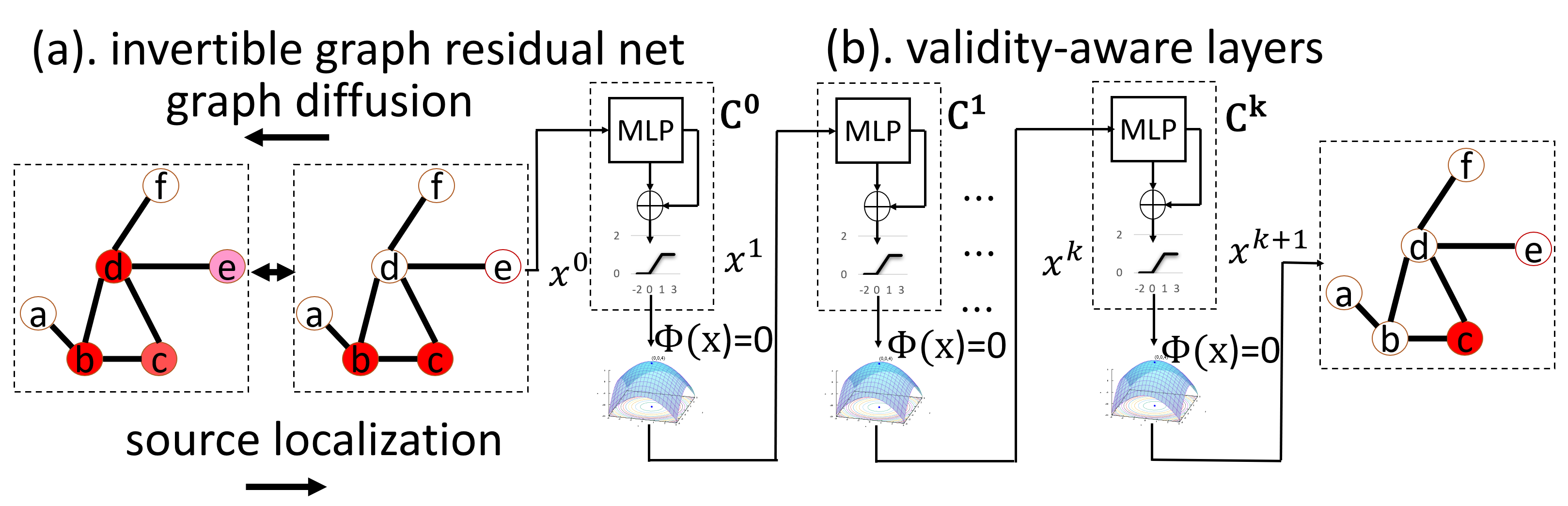
Figure 2. Framework overview: the proposed IVGD framework consists of an invertible graph diffusion model and a series of validity-aware layers.

Algorithm 1 Inverse of the Graph Residual Net for Graph Source Localization

0:  $f_{W},g,Y_{T},m$ {the number of iterations}.

0:  $z$ {an estimation of the source vector $x$}.

1:  $\zeta^{0}=Y_{T}$ {Initialization of label propagation}

2:  for i=1 to m do

3:     $\zeta^{i}=2Y_{T}-g(\zeta^{i-1})$ {Fix point iteration of label propagation}

4:  end for

5:  $z^{0}=\zeta^{m}$ {Initialization of feature construction}

6:  for i=1 to m do

7:     $z^{i}=2\zeta^{m}-f_{W}(z^{i-1})$ {Fix point iteration of feature construction}

8:  end for

9:  Output $z$.

Next, we provide theoretical guarantees on the invertibility of the graph residual net. Specifically, we prove a sufficient condition to ensure invertibility and discuss practical issues to satisfy such conditions. The following theorem provides a sufficient condition for the invertibility of the graph residual net.

Theorem 4.1 (Sufficient Condition for the invertibility of the graph residual net).

The graph residual net $P$ is invertible if $L_{f}<1$ and $L_{g}<1$, where $L_{f}$ and $L_{g}$ are Lipschitz constants of $f_{W}(x)$ and $g(\zeta)$, respectively.

Proof.

Because $P=G(F_{W})$, $P$ is invertible if $F_{W}$ and $G$ are invertible. We have $x=2\zeta-f_{W}(x)$ and $\zeta=2Y_{T}-g(\zeta)$ by the definitions of $F_{W}$ and $G$, and rewrite them as iterations as follows:

$$x^{0}=\zeta\ \text{and}\ x^{k+1}=2\zeta-f_{W}(x^{k})$$

$$\zeta^{0}=Y_{T}\ \text{and}\ \zeta^{k+1}=2Y_{T}-g(\zeta^{k})$$

where $\lim\nolimits_{k\rightarrow\infty}x^{k}=x$ and $\lim\nolimits_{k\rightarrow\infty}\zeta^{k}=\zeta$ are fixed points if $x^{k}$ and $\zeta^{k}$ converge. Because $f_{W}$ and $g$ are operators on a Banach space, $L_{f}<1$ and $L_{g}<1$ guarantee convergence by the Banach fixed point theorem (behrmann2019invertible, ). ∎

Then the following lemma provides the upper bound of the Lipschitz constants of the graph residual net.

Lemma 4.2 (The Lipschitz constants of the graph residual net).

Let $L_{P}$ and $L_{P^{-1}}$ be Lipschitz constants of $P$ and $P^{-1}$, respectively, then $L_{P}\leq\frac{(1+L_{f})(1+L_{g})}{4}$, and $L_{P^{-1}}\leq\frac{4}{(1-L_{f})(1-L_{g})}$.

Sketch of Proof.

To prove this lemma, we need to show that for any $x^{{}^{\prime}},x^{{}^{\prime\prime}},\|P(x^{{}^{\prime\prime}})-P(x^{{}^{\prime}})\|\leq\frac{(L_{f}+1)(L_{g}+1)}{4}\|x^{{}^{\prime\prime}}-x^{{}^{\prime}}\|$, and for any $y^{{}^{\prime}},y^{{}^{\prime\prime}},\|P^{-1}(y^{{}^{\prime\prime}})-P^{-1}(y^{{}^{\prime}})\|\leq\frac{4}{(1-L_{f})(1-L_{g})}\|y^{{}^{\prime\prime}}-y^{{}^{\prime}}\|$. The complete proof is shown in Section A in the appendix. ∎

Based on Theorem 4.1 and Lemma 4.2, we conclude that the Lipschitz constant of $P$ is less than 1 and therefore $P$ is invertible. Now we briefly discuss how to guarantee the Lipschitz constraints in practice. For $F_{W}$, which contains a set of learnable weights $W$, the power iteration method can be applied to normalize $W$ so that its norm is smaller than 1 (gouk2021regularisation, ). For $G$, many classical propagation functions such as the Independent Cascade (IC) function satisfies this condition (xia2021DeepIS, ).

4.2. Validity-aware Layers

The invertible graph residual net provides an estimation of source localization, However, the validity constraint $\Phi(x)=0$ is still required to satisfy. Specifically, we aim to resolve the following optimization problem:

(2) $$\min\nolimits_{x}R(x)\quad s.t.\quad x=C(z),\quad\Phi(x)=0.$$

where $R(x)$ is a loss function, and $z$ is the output of the graph residual net in Algorithm 1. However, Equation (2) is unsolvable due to the potential constraint conflict $x=C(z)$ and $\Phi(x)=0$. To address this, Equation (2) is reduced to the following optimization problem:

(3) $$\min\nolimits_{x}R(x)+\frac{\tau}{2}\|x-C(z)\|^{2}_{2}\ \ s.t.\ \Phi(x)=0.$$

where $\tau>0$ is a tuning parameter to balance the loss and the error compensation module. Then the task here is to design activation layers, in order to solve Equation (3). While traditional activation layers focus on individual nodes, and cannot handle difficult constraints, unrolled optimization techniques are potential ways to incorporate complex validity patterns into the model. Motivated by the recent development of ADMM-Net (sun2016deep, ) and OptNet (Amos2017OptNet, ), a potential solution to Equation (3) can be achieved by unrolling the problem into a neural net, where each layer is designed for the following optimization problem:

(4) $$x^{k+1} \leftarrow\arg\min\nolimits_{x}J^{k}(x)\ s.t.\ \Phi(x)=0,$$

where $J^{k}(x)=R(x)+\frac{\tau^{k}}{2}\|x-C^{k}(x^{k})\|^{2}_{2}$ and $x^{0}=z$. $x^{k}$ and $x^{k+1}$ are the input and the output of the $k$-th layer, respectively. To solve Equation (4), the augmented Lagrangian function is formulated mathematically as follows (bertsekas2014constrained, ):

$$H^{k}(x,\lambda)=J^{k}(x)+\Psi^{k}(x,\lambda),$$

where $\Psi^{k}(x,\lambda)=\frac{1}{2\rho^{k}}((\lambda+\rho^{k}\Phi(x))^{2}-\lambda^{2})$, $\rho>0$ is a hyperparameter, and $\lambda$ is a dual variable to address $\Phi(x)=0$. To optimize $H^{k}(x,\lambda)$, the OptNet updates variables via the implicit gradients of the Karush–Kuhn–Tucker (KKT) conditions (Amos2017OptNet, ). However, its computational efficiency is limited due to the nonconvexity and nonlinearity of $\Phi(x)$, and scales poorly on the large-scale networks (i.e. Challenge 3 in Section 3.2). To address this, we utilize a linearization technique to transform the nonconvex $H^{k}(x,\lambda)$ to the convex $h^{k}(x)$ as follows (yang2013linearized, ):

$$h^{k}(x) =J^{k}(x)+\!\partial_{x}(\Psi^{k})^{T}(x^{k},\lambda^{k})(x-x^{k})+\frac{\alpha^{k}}{2}\|x-x^{k}\|^{2}_{2},$$

where $\alpha^{k}>0$ is a hyperparameter to control the quadratic term. We formulate the validity-aware layer as follows:

$$x^{k+1} \leftarrow\arg\min\nolimits_{x}h^{k}(x),$$

$$\lambda^{k+1} \leftarrow\lambda^{k}+\rho^{k}\Phi(x^{k+1}).$$

Specifically, $C^{k},\rho^{k},\tau^{k},\alpha^{k}$ can be considered as learnable parameters of the $k$-th layer. Notice that if $R(x)$ is a mean square error, then $h^{k}(x)$ is quadratic and has a closed-form solution. Validity-aware layers can be trained by state-of-the-art optimizers such as SGD and Adam (Diederik2015Adam, ).

4.3. Convergence of the Proposed IVGD

Like other unrolled optimization models which solve objective functions effectively, our proposed IVGD can address Equation (3) by closed-form solutions. However, there lacks an understanding of the convergence of unrolled optimization models. This is because they usually involve many learnable parameters, which complicate the investigation of convergence. In this section, we provide the convergence guarantees of the proposed IVGD for the linear constraint $\Phi(x)=Ax-b$ where $A$ and $b$ are a given matrix and vector, respectively. Specifically, we propose a novel condition based on learnable parameters to ensure $x^{k}$ and $\lambda^{k}$ are closer to a solution as layers go deeper. Due to the space limit, we show the sketches of all proofs, and the complete proofs are available in the appendix.
The optimality conditions of Equation (4) are shown as follows:

$$Ax^{k}_{*}-b=0,\ \nabla J^{k}(x^{k}_{*})+A^{T}\lambda^{k}_{*}=0,$$

where $(x^{k}_{*},\lambda^{k}_{*})$ is an optimal solution (not necessarily unique) to Equation (4), which depends on $\tau^{k}$ and $C^{k}$. The following lemma provides the relationship between $(x^{k}_{*},\lambda^{k}_{*})$ and $(x^{k+1},\lambda^{k+1})$.

Lemma 4.3.

For any $k\in\mathbb{N}$, it satisfies

$$\frac{1}{\rho^{k}}(\lambda^{k}-\lambda^{k+1})^{T}(\lambda^{k+1}-\lambda^{k}_{*})+\alpha^{k}(x^{k}-x^{k+1})^{T}(x^{k+1}-x^{k}_{*})$$

$$\geq(x^{k+1}-x^{k})^{T}A^{T}(\lambda^{k}-\lambda^{k+1}).$$

Sketch of Proof.

It can be obtained by the optimality conditions of $x^{k+1}$ and $x^{k}_{*}$. The complete proof is shown in Section B in the appendix. ∎

Motivated by Lemma 4.3, we let $u_{1}=(x_{1},\lambda_{1})$ and $u_{2}=(x_{2},\lambda_{2})$, and define an inner product by

(5) $$\langle u_{1},u_{2}\rangle_{M^{k}}=\frac{1}{\rho^{k}}\lambda_{1}^{T}\lambda_{2}+\alpha^{k}x^{T}_{1}x_{2}.$$

and the induced norm $\|u\|^{2}_{M^{k}}=\langle u,u\rangle_{M^{k}}$. Denote $u^{k}_{*}=(x^{k}_{*},\lambda^{k}_{*})$ and $u^{k}=(x^{k},\lambda^{k})$. The following theorem states that $u^{k+1}$ is a feasible solution to Equation (4).

Theorem 4.4 (Asymptotic Convergence).

Assume $0<D_{1}\leq\alpha^{k}\leq D_{2}<\infty$, $0<D_{3}\leq\rho^{k}\leq D_{4}<\infty$ and $\alpha^{k}-\rho^{k}r(A^{T}A)>0$ where $D_{1}$, $D_{2}$, $D_{3}$ and $D_{4}$ are constant, and $r(A^{T}A)$ denotes the spectral radius of $A^{T}A$. If there exists $(C^{k},\rho^{k},\tau^{k},\alpha^{k})$ such that $\|u^{k+1}-u^{k+1}_{*}\|^{2}_{M^{k+1}}\leq\|u^{k+1}-u^{k}_{*}\|^{2}_{M^{k}}$, then we have
(a). $\|u^{k}-u^{k+1}\|^{2}_{M^{k}}\rightarrow 0$.
(b). $\|u^{k}-u^{k}_{*}\|^{2}_{M^{k}}$ is nonincreasing and hence converges.
(c). $u^{k+1}$ is a feasible solution to Equation (4) . That is,
$\lim\nolimits_{k\rightarrow\infty}Ax^{k+1}\!-\!b=0$, $\lim\nolimits_{k\rightarrow\infty}\nabla J^{k}(x^{k+1})\!+\!A^{T}\lambda^{k+1}\!=\!0$.

Sketch of Proof.

To prove this theorem, we need to show that $\|u^{k}-u^{k}_{*}\|^{2}_{M^{k}}\geq\|u^{k+1}-u^{k+1}_{*}\|^{2}_{M^{k+1}}+\mu^{k}\|u^{k+1}-u^{k}\|^{2}_{M^{k}}$ where $\mu^{k}>0$, which can be obtained by Lemma 4.3. The complete proof is in Section C in the appendix. ∎

The condition $\|u^{k+1}-u^{k+1}_{*}\|^{2}_{M^{k+1}}\leq\|u^{k+1}-u^{k}_{*}\|^{2}_{M^{k}}$ guarantees there exist learnable parameters to make $u^{k+1}$ contractive with respect to the norm induced by $M^{k}$. Theorem 4.4 ensures that the gap between $u^{k+1}$ and $u^{k}$ converges to $0$, and $u^{k+1}$ converges to a feasible solution to Equation (4) with constraint satisfaction $\lim\nolimits_{k\rightarrow\infty}Ax^{k+1}-b=0$.

5. Experiment Verification

In this section, nine real-world datasets were utilized to test our proposed IVGD compared with state-of-the-art methods. Performance evaluation, ablation studies, sensitivity analysis, and scalability analysis have demonstrated the effectiveness, robustness, and efficiency of the proposed IVGD. All experiments were conducted on a 64-bit machine with Intel(R) Xeon(R) quad-core processor (W-2123 CPU@ 3.60 GHZ) and 32.0 GB memory.

5.1. Experimental Protocols

5.1.1. Data Description

We compare our proposed IVGD with the state-of-the-art methods on nine real-world datasets in the experiments, whose statistics are shown in Table 2. Due to space limit, their descriptions are outlined in Section D in the Appendix. The Deezer dataset was only used to evaluate the scalability.
For all datasets except the Memetracker and the Digg, we generated diffusion cascades based on the following strategy: $10\%$ nodes were chosen as source nodes randomly, and then the diffusion was repeated 60 times for each source vector. For each cascade, we have a source vector $x$ and a diffusion vector $Y_{T}$. For the Memetracker and Digg, they provided true source vectors and diffusion vectors. The ratio of the sizes of the training set and the test set was 8:2.

5.1.2. Comparison Methods

For comparison methods, three state-of-the-art approaches LPSI (wang2017multiple, ), NetSleuth (prakash2012spotting, ) and GCNSI (dong2019multiple, ) are compared with our proposed IVGD, all of which are outlined as follows:
1. LPSI (wang2017multiple, ). LPSI is short for Label Propagation based Source Identification. It is inspired by the label propagation algorithm in semi-supervised learning.
2. NetSleuth (prakash2012spotting, ). The goal of NetSleuth is to employ the Minimum Description Length principle to identify the best set of source nodes and virus propagation ripple (prakash2012spotting, ).
3. GCNSI (dong2019multiple, ). GCNSI is a Graph Convolutional Network (GCN) based source identification algorithm. It used the LPSI to augment input, and then applied the GCN for source identification.

Name	#Nodes	#Edges	Average Degree	Diameter
Karate	34	78	2.294	5
Dolphins	62	159	5.129	8
Jazz	198	2,742	13.848	9
Network Science	1,589	2,742	3.451	17
Cora-ML	2,810	7,981	5.68	17
Power Grid	4,941	6,594	2.669	46
Memetracker	1,653	4,267	5.432	4
Digg	11,240	47,885	8.52	4
Deezer	47,538	222,887	9.377	-

Table 2. Statistics of nine real-world datasets.

5.1.3. Metrics

Five metrics were applied to evaluate the performance: the Accuracy (ACC) is the ratio of accurately labeled nodes to all nodes; the Precision (PR) is the ratio of accurately labeled as source nodes to all nodes labeled as source; the Recall (RE) defines the ratio of accurately labeled as source nodes to all true source nodes; the F-Score (FS) is the harmonic mean of Precision and Recall, which is the most important metric for performance evaluation. This is because the proportion of source nodes is far smaller than that of other nodes (i.e. label imbalance). Besides, the Area Under the Receiver operating characteristic curve (AUC) is an important metric to evaluate a classifier given different thresholds.

5.1.4. Parameter Settings

For the proposed IVGD, the $f_{W}(x)$ was chosen to be a 2-layer MLP model, where the number of hidden units was set to 6 for all datasets except Memetracker and Digg (xia2021DeepIS, ). It was set to $100$ and $50$ for Memetracker and Digg, respectively. $g(\zeta)$ was chosen to be the IC function, the number of validity-aware layers was set to 10. The error compensation module was a three-layer MLP model, where the number of neurons was 1,000. $\alpha$, $\tau$ and $\rho$ were set to $1$, $10$ and $10^{-3}$, respectively based on the optimal training performance. The learning rate of the SGD was set to $10^{-3}$. The number of the epoch was set to $100$. The equality constraint we used was $\|x\|_{0}=|S|$, which means that the number of source nodes was known in advance. However, it is non-differentiable and nonconvex. To address this, we relaxed the constraint to a linear constraint as follows: $\sum\nolimits_{i=1}^{n}x_{i}=|S|$. This constraint was only used in the training phase.
For all comparison methods, the $\alpha$ in LPSI and GCNSI was set to $0.01$ and $0.49$, respectively, based on the optimal training performance. The GCN in GCNSI was a two-layer architecture, where the number of hidden neurons was 128. The learning rate in SGD was set to $10^{-3}$.

	Karate				Dolphins
Method	ACC	PR	RE	FS	ACC	PR	RE	FS
LPSI	0.9559	0.6800	1.0000	0.7970	0.9677	0.7790	1.0000	0.8717
NetSleuth	0.9147	0.5371	0.6833	0.5965	0.9306	0.6454	0.7425	0.6904
GCNSI	0.7088	0.1150	0.2667	0.1581	0.6177	0.1015	0.2548	0.1372
IVGD(ours)	0.9853	0.8717	1.0000	0.9213	0.9935	0.9444	1.0000	0.9701
	Network Science				Cora-ML
Method	ACC	PR	RE	FS	ACC	PR	RE	FS
LPSI	0.9831	0.8525	1.0000	0.9202	0.9011	0.5067	0.9993	0.6724
NetSleuth	0.9595	0.7642	0.8429	0.8016	0.8229	0.1627	0.1793	0.1706
GCNSI	0.8840	0.0582	0.0135	0.0218	0.8580	0.0970	0.0478	0.0637
IVGD(ours)	0.9946	0.9476	1.0000	0.9730	0.9973	0.9744	1.0000	0.9870
	Jazz				Power Grid
Method	ACC	PR	RE	FS	ACC	PR	RE	FS
LPSI	0.9035	0.6074	0.9944	0.7371	0.9673	0.7584	1.0000	0.8624
NetSleuth	0.9222	0.5904	0.6629	0.6245	0.9276	0.6347	0.6986	0.6651
GCNSI	0.7525	0.0685	0.1280	0.0849	0.7125	0.1022	0.2285	0.1410
IVGD(ours)	0.9980	0.9802	1.0000	0.9899	0.9902	0.9133	1.0000	0.9546

Table 3. Test performance of simulations on six datasets: the proposed IVGD dominates in all methods on six datasets.

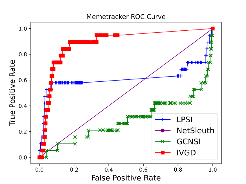
(a). Memetracker

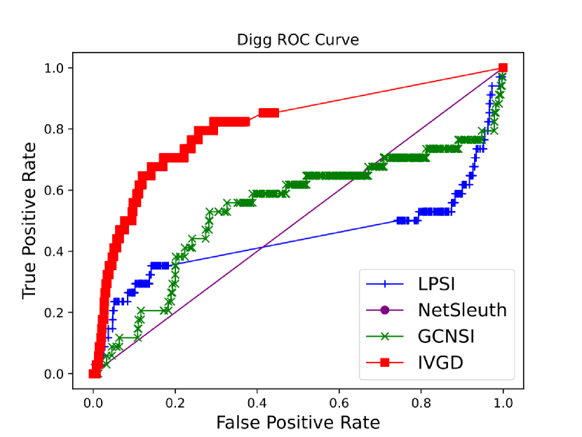
(b). Digg

Figure 3. ROC curves on two real-world datasets: all comparison methods are surrounded by the proposed IVGD.

5.2. Performance Evaluation

The test performance of all methods on six datasets is demonstrated in Table 3. The best performance is highlighted in bold. Overall, our proposed IVGD outperforms all comparison methods significantly on all datasets. Specifically, the ACCs of the proposed IVGD on six datasets are all above $0.98$, and the PRs are also above $0.9$. Most importantly, the FS metric of the proposed IVGD is in the vicinity of $0.96$ on average. This substantiates that our proposed IVGD algorithm can accurately predict source nodes despite their scarcity. For comparison methods, the LPSI performs the best followed by NetSleuth: the ACCs of the LPSI are $2\%$ higher than those of NetSleuth, and the PRs are around $10\%$ better. For example, our proposed IVGD attains 0.99 and 0.95 in the ACC and the PR on the Power Grid dataset, respectively, while the counterparts of the LPSI are 0.97 and 0.86, respectively, and the NetSleuth achieves 0.62 and 0.65, respectively. The GCNSI performs poorly on all datasets: its PRs and FSes are surprisingly low, which are below 0.3. For instance, the PR and the FS on the Network Science dataset are 0.08 and 0.03, respectively. This is because it cannot differentiate source nodes from others, and its predictions are in the vicinity of the threshold. This demonstrates that the GCNSI cannot draw a clear decision boundary.

	Karate				Dolphins
Method	ACC	PR	RE	FS	ACC	PR	RE	FS
IVGD(1)	0.9618	0.7167	1.0000	0.8248	0.9694	0.7873	1.0000	0.8774
IVGD(2)	0.9882	0.8967	1.0000	0.9356	0.9726	0.8070	1.0000	0.8904
IVGD(3)	0.9500	0.6583	1.0000	0.7824	0.9613	0.7519	1.0000	0.8517
IVGD	0.9853	0.8717	1.0000	0.9213	0.9935	0.9444	1.0000	0.9701
	Network Science				Cora-ML
Method	ACC	PR	RE	FS	ACC	PR	RE	FS
IVGD(1)	0.9859	0.8736	1.0000	0.9324	0.8712	0.4411	1.0000	0.6121
IVGD(2)	0.9867	0.8799	1.0000	0.9360	0.9959	0.9617	1.0000	0.9805
IVGD(3)	0.9812	0.8383	1.0000	0.9119	0.9850	0.8717	1.0000	0.9314
IVGD	0.9946	0.9476	1.0000	0.9730	0.9973	0.9744	1.0000	0.9870
	Jazz				Power Grid
Method	ACC	PR	RE	FS	ACC	PR	RE	FS
IVGD(1)	0.9586	0.7092	1.0000	0.8266	0.9729	0.7916	1.0000	0.8835
IVGD(2)	0.9904	0.9123	1.0000	0.9528	0.9881	0.8967	1.0000	0.9455
IVGD(3)	0.9646	0.7394	1.0000	0.8473	0.9631	0.7358	1.0000	0.8475
IVGD	0.9980	0.9802	1.0000	0.9899	0.9902	0.9133	1.0000	0.9546

Table 4. Ablation studies on simulations of six test datasets: all components in our model contribute to the outstanding performance.

Aside from simulations, we also evaluate our proposed IVGD on two real-world datasets, as shown in Figure 3. X-axis and Y-axis represent the true positive rate and the false positive rate, respectively. Similarly as Table 3, our proposed IVGD also outperforms others significantly on the ROC curves: all comparison methods are surrounded by our proposed IVGD. Specifically, the AUCs of our proposed IVGD are above $0.6$ on the Memetracker and the Digg datasets, whereas these of all other methods are either around $0.5$ or below $0.5$. The LPSI outperforms the GCNSI by about $20\%$ on the Memetracker, while it performs worse on the Digg by $10\%$.

5.3. Ablation Studies

One important question to our proposed IVGD is whether all components in our model are necessary. To investigate this, we test our performance on six datasets, when some components are removed. For the sake of simplicity, IVGD(1) means that the invertible graph residual net was removed, IVGD(2) means that the error compensation module was removed, and IVGD(3) means that validity-aware layers were removed. The results on six datasets are demonstrated in Table 4. Overall, the performance will degrade if any component of our proposed IVGD is removed. Without the invertible graph residual net, the performance on the Cora-ML dataset drops significantly from $99.7\%$ to $87\%$ in the ACC, and the PR has declined by more than $50\%$. The FS on the Power Grid has demonstrated a $7\%$ drop due to the same reason. Validity-aware layers provide a giant leap on FS when we compare IVGD(3) with IVGD. The performance of the FS has been enhanced by $5\%-14\%$. For example, the FS on the Power Grid dataset soars from $0.848$ to $0.955$. The same pattern is applied to the Karate and the Dolphins datasets. This suggests that integrating validity patterns into the model significantly improves model performance. The error compensation module plays a less important role than the invertible graph residual net and validity-aware layers. Specifically, the performance drop without it is slim compared with other components. For example, the drop of the ACC on the Jazz dataset is less than $1\%$. Moreover, the ACC on the Karate dataset even increases slightly. But the effect of the error compensation module is still positive overall.

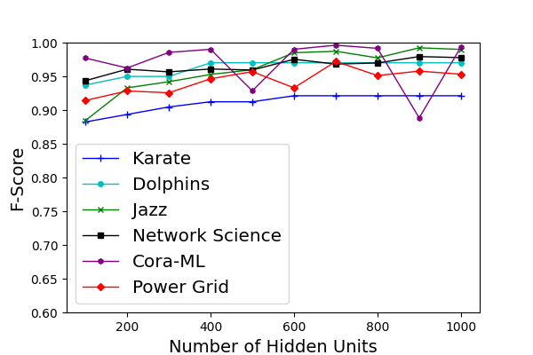
(a). Hidden units VS FS.

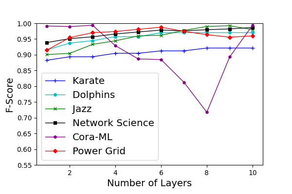
(b). Layers VS FS.

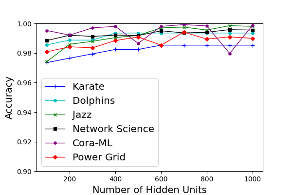
(c). Hidden units VS ACC.

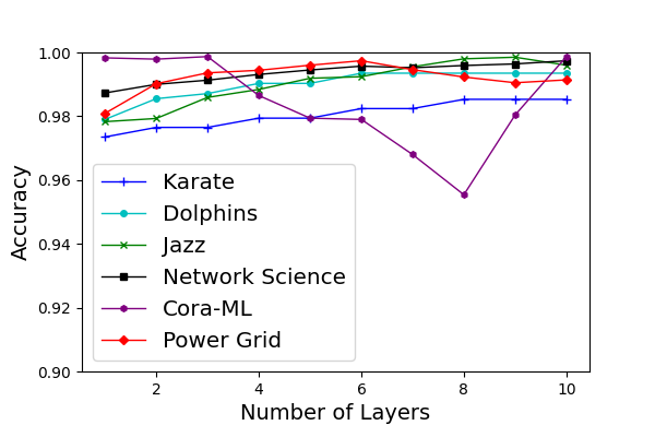
(d). Layers VS ACC.

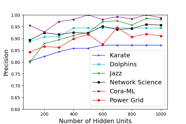
(e). Hidden units VS PR.

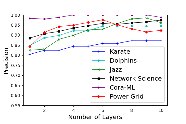
(f). Layers VS PR.

Figure 4. The impacts of two factors on the FS, ACC and PR: more hidden units and layers lead to better performance.

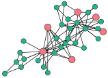
(a) LPSI

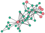
(b) NetSleuth

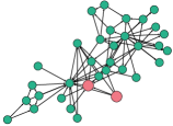
(c) GCNSI

(d) IVGD

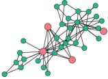
(e) True Sources

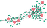
(f) LPSI

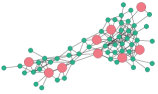
(g) NetSleuth

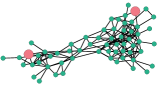
(h) GCNSI

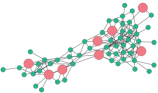
(i) IVGD

(j) True Sources

Figure 5. Visualizations of two datasets for all methods and true source patterns. Figures 5a - 5e are visualizations of Karate, and Figures 5f - 5j are visualizations of Dolphins. Sources nodes and other nodes are marked with red and green, respectively.

5.4. Sensitivity Analysis

Next, it is crucial to investigate how parameter settings affect performance. In this section, we explore two factors: the number of hidden units in the compensation module and the number of validity-aware layers. The number of epochs was set to 10. For the hidden units, we changed the number from $100$ to $1,000$; for the layers, the number ranged from 1 to 10. The impacts on FS, ACC, and PR are shown in Figure 4. Overall, the performance increases smoothly with the increase of hidden units and layers. For example, the FS on the Network Science dataset increases by $2\%$ when hidden units are changed from $100$ to $1,000$; it climbs by $4\%$ when the layers ranged from $1$ to $10$. However, there is an exception: the FS fluctuates on the Cora-ML dataset. The amplitudes are about $10\%$ and $30\%$ for hidden units and layers, respectively. Despite the fluctuation, the lowest FSes achieved by 800 hidden units and seven layers are still better than all comparison methods, as shown in Table 3.

5.5. Scalability Analysis

Method	Karate	Dolphins	Jazz	Network Science	Cora-ML	Power Grid	Deezer
LPSI	0.26	0.27	0.76	52.83	240.88	899.45	94541.13
NetSleuth	0.33	0.48	1.95	32.96	645.04	1260.68	114425.32
GCNSI	1.55	34.62	125.59	283.62	776.70	2324.53	174923.31
IVGD(ours)	5.37	6.45	9.78	23.95	92.68	177.32	46832

Table 5. The running time (seconds) on simulations of seven datasets: our proposed IVGD runs the most efficiently on the large-scale networks.

To test the efficiency and scalability of our proposed IVGD, we compared the running time of IVGD with all comparison methods on seven datasets, which is shown in Table 5. The best running time is highlighted in bold. In general, we proposed IVGD runs the most efficiently on large-scale networks such as Deezer, which consists of about $5,0000$ nodes. Specifically, it consumes about half a day to finish training, while all comparison methods at least double. The same trend holds in other large networks such as Cora-ML and Power Grid. The LPSI takes the least time on small networks such as Karate and Dolphins. The GCNSI is the slowest method on most datasets. For example, it consumes around 2 minutes on the small Jazz dataset, while all other methods take less than 10 seconds. It takes 2 days on the Deezer dataset, whereas the LPSI only requires half of that time.

5.6. Invertibility Analysis

For the invertibility, one may raise a concern on whether it impairs the performance of graph diffusion models. To investigate this question, we compare the performance of the GNN model $\theta$ and the proposed Invertible Graph Residual Net (IGRN) $P$ on eight datasets. The DeepIS (xia2021DeepIS, ) was chosen as the GNN model, and the IGRN was implemented based on the DeepIS. The Mean Square Error (MSE) and the Mean Absolute Error (MAE) were used to assess the performance. Table 6 illustrates the performance of two graph diffusion models. In summary, they perform similarly on two metrics across different datasets. Specifically, the GNN achieves a better performance on the Karate, Dolphins, Cora-ML, and Power Grid datasets, whereas the IGRN stands out on the Dolphins, Network Science, Memetracker, and Digg datasets. The largest gap comes from the MAE on the Karate dataset, where the GNN outperforms IGRN by $0.02$.

	Karate		Dolphins		Jazz		Network Science
	MSE	MAE	MSE	MAE	MSE	MAE	MSE	MAE
GNN	0.0287	0.0773	0.0270	0.1063	0.0575	0.1731	0.0199	0.0743
IGRN	0.0311	0.1010	0.0258	0.0794	0.0514	0.1867	0.0156	0.0643
	Cora-ML		Power Grid		Memetracker		Digg
	MSE	MAE	MSE	MAE	MSE	MAE	MSE	MAE
GNN	0.0017	0.0282	0.0221	0.0633	0.0273	0.0322	0.0198	0.0265
IGRN	0.0041	0.0488	0.0247	0.0758	0.0236	0.0311	0.0165	0.0203

Table 6. The effect of invertibility on graph diffusion models: it plays a negligible role.

5.7. Visualization

Finally, we demonstrate the effectiveness of our proposed IVGD by visualizing two small datasets Karate and Dolphin in Figure 5. Red nodes and green nodes represent source nodes and other nodes, respectively. Specifically, our proposed IVGD perfectly predicts all sources on two datasets, and the LPSI and the NetSleuth also achieve similar source patterns as the ground truth: they only misclassify several source nodes. The GCNSI, however, misses most of the source nodes. This is because it suffers from class imbalance problems, and tends to classify none of all nodes as a source node. This is consistent with test performance shown in Table 3.

6. Conclusion

Graph source localization is an important yet challenging problem in graph mining. In this paper, we propose a novel Invertible Validity-aware Graph Diffusion (IVGD) to address this problem from the perspective of the inverse problem. Firstly, we propose an invertible graph residual net by restricting its Lipschitz constant with guarantees. Moreover, we present an error compensation module to reduce the introduced errors with skip connection. Finally, we utilize the unrolled optimization technique to impose validity constraints on the model. A linearization technique is used to transform problems into solvable forms. We provide the convergence of the proposed IVGD to a feasible solution. Extensive experiments on nine real-world datasets have demonstrated the effectiveness, robustness, and efficiency of our proposed IVGD.

Appendix

Appendix A The proof of Lemma 4.2

Proof.

On one hand, for any $x^{{}^{\prime}},x^{{}^{\prime\prime}}$, we have

$$\|P(x^{{}^{\prime\prime}})-P(x^{{}^{\prime}})\|=\|G(F_{W}(x^{{}^{\prime\prime}}))-G(F_{W}(x^{{}^{\prime}}))\|=\|\frac{g(F_{W}(x^{{}^{\prime\prime}}))+F_{W}(x^{{}^{\prime\prime}})}{2}-\frac{g(F_{W}(x^{{}^{\prime}}))+F_{W}(x^{{}^{\prime}})}{2}\|$$

$$\leq\frac{1}{2}\|g(F_{W}(x^{{}^{\prime\prime}}))-g(F_{W}(x^{{}^{\prime}}))\|+\frac{1}{2}\|F_{W}(x^{{}^{\prime\prime}})-F_{W}(x^{{}^{\prime}})\|\ (\text{triangle inequality})$$

$$\leq\frac{L_{g}+1}{2}\|F_{W}(x^{{}^{\prime\prime}})-F_{W}(x^{{}^{\prime}})\|\ (\text{Lipschitz constant of $g$})$$

$$=\frac{L_{g}+1}{4}\|f_{W}(x^{{}^{\prime\prime}})+x^{{}^{\prime\prime}}-f_{W}(x^{{}^{\prime}})-x^{{}^{\prime}}\|$$

$$\leq\frac{L_{g}+1}{4}(\|f_{W}(x^{{}^{\prime\prime}})-f_{W}(x^{{}^{\prime}})\|+\|x^{{}^{\prime\prime}}-x^{{}^{\prime}}\|)\ \text{(triangle inequality)}$$

$$\leq\frac{(L_{f}+1)(L_{g}+1)}{4}\|x^{{}^{\prime\prime}}-x^{{}^{\prime}}\|\ (\text{Lipschitz constant of $f_{w}$}).$$

This suggests that $L_{P}\leq\frac{(L_{f}+1)(L_{g}+1)}{4}$. On the other hand,

$$\|P(x^{{}^{\prime\prime}})-P(x^{{}^{\prime}})\|=\|\frac{g(F_{W}(x^{{}^{\prime\prime}}))+F_{W}(x^{{}^{\prime\prime}})}{2}-\frac{g(F_{W}(x^{{}^{\prime}}))+F_{W}(x^{{}^{\prime}})}{2}\|$$

$$\geq\frac{1}{2}\|F_{W}(x^{{}^{\prime\prime}})-F_{W}(x^{{}^{\prime}})\|-\frac{1}{2}\|g(F_{W}(x^{{}^{\prime\prime}}))-g(F_{W}(x^{{}^{\prime}}))\|\ (\text{triangle inequality})$$

$$\geq\frac{1-L_{g}}{2}\|F_{W}(x^{{}^{\prime\prime}})-F_{W}(x^{{}^{\prime}})\|\ (\text{Lipschitz constant of $g$})$$

$$=\frac{1-L_{g}}{4}\|f_{W}(x^{{}^{\prime\prime}})+x^{{}^{\prime\prime}}-f_{W}(x^{{}^{\prime}})-x^{{}^{\prime}}\|$$

$$\geq\frac{1-L_{g}}{4}(\|x^{{}^{\prime\prime}}-x^{{}^{\prime}}\|-\|f_{W}(x^{{}^{\prime\prime}})-f_{W}(x^{{}^{\prime}})\|)\ \text{(triangle inequality)}$$

$$\geq\frac{(1-L_{f})(1-L_{g})}{4}\|x^{{}^{\prime\prime}}-x^{{}^{\prime}}\|\ (\text{Lipschitz constant of $f_{w}$}).$$

Let $y^{{}^{\prime}}=P(x^{{}^{\prime}})$, $y^{{}^{\prime\prime}}=P(x^{{}^{\prime\prime}})$, so $x^{{}^{\prime}}=P^{-1}(y^{{}^{\prime}})$, $x^{{}^{\prime\prime}}=P^{-1}(y^{{}^{\prime\prime}})$. This leads to $\|P^{-1}(y^{{}^{\prime\prime}})-P^{-1}(y^{{}^{\prime}})\|\leq\frac{4}{(1-L_{f})(1-L_{g})}\|y^{{}^{\prime\prime}}-y^{{}^{\prime}}\|.$ This suggests that $L_{P^{-1}}\leq\frac{4}{(1-L_{f})(1-L_{g})}$, and it concludes the proof. ∎

Appendix B The Proof of Lemma 4.3

Proof.

The optimality condition of $x^{k+1}$ leads to $\nabla J^{k}(x^{k+1})+A^{T}\lambda^{k}+\rho^{k}A^{T}(Ax^{k}-b)+\alpha^{k}(x^{k+1}-x^{k})=0.$ We plug in $\lambda^{k+1}=\lambda^{k}+\rho^{k}(Ax^{k+1}-b)$ and arrange to obtain

(6) $$\nabla J^{k}(x^{k+1})+A^{T}\lambda^{k+1}-\rho^{k}A^{T}A(x^{k+1}-x^{k})+\alpha^{k}(x^{k+1}-x^{k})=0.$$

That is $\nabla J^{k}(x^{k+1})=-A^{T}\lambda^{k+1}+\rho^{k}A^{T}A(x^{k+1}-x^{k})-\alpha^{k}(x^{k+1}-x^{k}).$ Also the optimality condition of $x^{k}_{*}$ results in $\nabla J^{k}(x^{k}_{*})+A^{T}\lambda^{k}_{*}=0$, due to the convexity of $J^{k}(x)$, we have

(7) $$J^{k}(x^{k+1})\geq J^{k}(x^{k}_{*})+(-A^{T}\lambda^{k}_{*})^{T}(x^{k+1}-x^{k}_{*}).$$

(8) $$J^{k}(x^{k}_{*})\geq J^{k}(x^{k+1})+(-A^{T}\lambda^{k+1}+\rho^{k}A^{T}A(x^{k+1}-x^{k})-\alpha^{k}(x^{k+1}-x^{k}))^{T}(x^{k}_{*}-x^{k+1}).$$

We sum Inequalities (7) and (8) to obtain $(A^{T}\lambda^{k+1}-A^{T}\lambda^{k}_{*}-\rho^{k}A^{T}A(x^{k+1}-x^{k})+\alpha^{k}(x^{k+1}-x^{k}))^{T}(x^{k}_{*}-x^{k+1})\geq 0.$ After rearranging terms, we have

$$(\lambda^{k+1}-\lambda^{k}_{*})^{T}A(x^{k}_{*}-x^{k+1})+\alpha^{k}(x^{k}-x^{k+1})^{T}(x^{k+1}-x^{k}_{*})\geq\rho^{k}(x^{k+1}-x^{k})^{T}A^{T}A(x^{k}_{*}-x^{k+1}).$$

Using the facts that $Ax^{k+1}-Ax^{k}_{*}=(Ax^{k+1}-b)-(Ax^{k}_{*}-b)=Ax^{k+1}-b=\frac{1}{\rho^{k}}(\lambda^{k+1}-\lambda^{k})$, and $a^{T}b=ab^{T}$($a$ and $b$ are two vectors), we have

$$\frac{1}{\rho^{k}}(\lambda^{k}-\lambda^{k+1})^{T}(\lambda^{k+1}-\lambda^{k}_{*})+\alpha^{k}(x^{k}-x^{k+1})^{T}(x^{k+1}-x^{k}_{*})\geq(x^{k+1}-x^{k})^{T}A^{T}(\lambda^{k}-\lambda^{k+1}).$$

∎

Appendix C Proof of Theorem 4.4

Proof.

We denote $u^{k}=(\lambda^{k},x^{k})$, $u^{k+1}=(\lambda^{k+1},x^{k+1})$, and $u^{k}_{*}=(\lambda^{k}_{*},x^{k}_{*})$. Using the notation defined in Equation (5), we have

$$\langle u^{k}-u^{k+1},u^{k+1}-u^{k}_{*}\rangle_{M^{k}}\geq(x^{k+1}-x^{k})^{T}A^{T}(\lambda^{k}-\lambda^{k+1}).$$

Because $u^{k+1}-u^{k}_{*}=u^{k+1}-u^{k}+u^{k}-u^{k}_{*}$, it follows that

(9) $$\langle u^{k}-u^{k+1},u^{k}-u^{k}_{*}\rangle_{M^{k}}\geq\|u^{k+1}-u^{k}\|^{2}_{M^{k}}+(x^{k+1}-x^{k})^{T}A^{T}(\lambda^{k}-\lambda^{k+1}).$$

It holds that

$$\|u^{k}-u^{k}_{*}\|^{2}_{M^{k}}-\|u^{k+1}-u^{k}_{*}\|^{2}_{M^{k}}$$

$$=2\langle u^{k}-u^{k+1},u^{k}-u^{k}_{*}\rangle_{M^{k}}-\|u^{k+1}-u^{k}\|^{2}_{M^{k}}$$

$$\geq\|u^{k+1}-u^{k}\|^{2}_{M^{k}}+2(x^{k+1}-x^{k})^{T}A^{T}(\lambda^{k}-\lambda^{k+1})(\text{Inequality \eqref{ineq: convex 3}})$$

$$=\frac{1}{\rho^{k}}\|x^{k+1}-x^{k}\|^{2}_{2}+\alpha^{k}\|\lambda^{k+1}-\lambda^{k}\|^{2}_{2}+2(x^{k+1}-x^{k})^{T}A^{T}(\lambda^{k}-\lambda^{k+1})\ (\text{the definition of $\|\bullet\|^{2}_{M^{k}}$})$$

$$=\frac{1}{\rho^{k}}\|x^{k+1}-x^{k}\|^{2}_{2}+\alpha^{k}\|\lambda^{k+1}-\lambda^{k}\|^{2}_{2}-2(A(x^{k+1}-x^{k}))^{T}(\lambda^{k+1}-\lambda^{k}).$$

Because $\alpha^{k}-\rho^{k}r(A^{T}A)>0$, it holds that $\delta^{k}=\frac{\alpha^{k}-\rho^{k}r(A^{T}A)}{2\rho^{k}r(A^{T}A)}>0$. Let $\eta^{k}=\frac{\alpha^{k}}{(1+\delta^{k})}>0$

$$\frac{1}{\rho^{k}}\|x^{k+1}-x^{k}\|^{2}_{2}+\alpha^{k}\|\lambda^{k+1}-\lambda^{k}\|^{2}_{2}-2(A(x^{k+1}-x^{k}))^{T}(\lambda^{k+1}-\lambda^{k})$$

$$\geq\frac{1}{\rho^{k}}\|x^{k+1}-x^{k}\|^{2}_{2}+\alpha^{k}\|\lambda^{k+1}-\lambda^{k}\|^{2}_{2}-\frac{1}{\eta^{k}}\|A(x^{k+1}-x^{k})\|^{2}_{2}-\eta^{k}\|\lambda^{k+1}-\lambda^{k}\|^{2}_{2}$$

$$(\text{$2(A(x^{k+1}-x^{k}))^{T}(\lambda^{k+1}-\lambda^{k})\leq\frac{1}{\eta^{k}}\|A(x^{k+1}-x^{k})\|^{2}_{2}+\eta^{k}\|\lambda^{k+1}-\lambda^{k}\|^{2}_{2}$})$$

$$\geq\frac{1}{\rho^{k}}\|x^{k+1}-x^{k}\|^{2}_{2}+\alpha^{k}\|\lambda^{k+1}-\lambda^{k}\|^{2}_{2}-\frac{r(A^{T}A)}{\eta^{k}}\|x^{k+1}-x^{k}\|^{2}_{2}-\eta^{k}\|\lambda^{k+1}-\lambda^{k}\|^{2}_{2}$$

$$(\|A(x^{k+1}-x^{k})\|^{2}_{2}\leq r(A^{T}A)\|x^{k+1}-x^{k}\|^{2}_{2}\ \text{where $r(A^{T}A)$ is the spectral radius of $A^{T}A$})$$

$$=(\frac{1}{\rho^{k}}-\frac{r(A^{T}A)}{\eta^{k}})\|x^{k+1}-x^{k}\|^{2}_{2}+(\alpha^{k}-\eta^{k})\|\lambda^{k+1}-\lambda^{k}\|^{2}_{2}$$

$$=\frac{\delta^{k}r(A^{T}A)}{\alpha^{k}}\|x^{k+1}-x^{k}\|^{2}_{2}+\frac{\alpha^{k}\delta^{k}}{1+\delta^{k}}\|\lambda^{k+1}-\lambda^{k}\|^{2}_{2}$$

$$\geq\mu^{k}\|u^{k+1}-u^{k}\|^{2}_{M^{k}}.$$

where $\mu^{k}=\min(\frac{\rho^{k}\delta^{k}r(A^{T}A)}{\alpha^{k}},\frac{\delta^{k}}{1+\delta^{k}})$ Because $(C^{k},\rho^{k},\tau^{k},\alpha^{k})$ guarantees that $\|u^{k+1}-u^{k+1}_{*}\|^{2}_{M^{k+1}}\leq\|u^{k+1}-u^{k}_{*}\|^{2}_{M^{k}}$, then we have

(10) $$\|u^{k}-u^{k}_{*}\|^{2}_{M^{k}}\geq\|u^{k+1}-u^{k}_{*}\|^{2}_{M^{k}}+\mu^{k}\|u^{k+1}-u^{k}\|^{2}_{M^{k}}\geq\|u^{k+1}-u^{k+1}_{*}\|^{2}_{M^{k+1}}+\mu^{k}\|u^{k+1}-u^{k}\|^{2}_{M^{k}}.$$

(a). We sum Inequality (10) from $k=0$ to $k=K$ to obtain

$$\sum\nolimits_{k=0}^{K}\mu^{k}\|u^{k+1}-u^{k}\|^{2}_{M^{k}}\leq\|u^{0}-u^{0}_{*}\|^{2}_{M^{0}}.$$

Let $K\rightarrow\infty$, we have $\lim\nolimits_{k\rightarrow\infty}\mu^{k}\|u^{k+1}-u^{k}\|^{2}_{M^{k}}=0$. Because $\mu^{k}>0$, we have $\lim\nolimits_{k\rightarrow\infty}\|u^{k+1}-u^{k}\|^{2}_{M^{k}}=0$.
(b). From Inequality (10), $\|u^{k}-u^{k}_{*}\|^{2}_{M^{k}}$ is nonincreasing, and $\|u^{k}-u^{k}_{*}\|^{2}_{M^{k}}>0$ has a lower bound. Therefore, $\|u^{k}-u^{k}_{*}\|^{2}_{M^{k}}$ is convergent.
(c). From (a) we know that $\lim\nolimits_{k\rightarrow\infty}\|u^{k+1}-u^{k}\|^{2}_{M^{k}}=0$. That is $\lim\nolimits_{k\rightarrow\infty}\frac{1}{\rho^{k}}\|x^{k+1}-x^{k}\|^{2}_{2}+\alpha^{k}\|\lambda^{k+1}-\lambda^{k}\|^{2}_{2}=0$. Because $\alpha^{k}\geq D_{1}>0$ and $\rho^{k}\leq D_{4}<\infty$, we have $\lim\nolimits_{k\rightarrow\infty}x^{k+1}-x^{k}=0$ and $\lim\nolimits_{k\rightarrow\infty}\lambda^{k+1}-\lambda^{k}=0$. Because $\lambda^{k+1}=\lambda^{k}+\rho^{k}(Ax^{k+1}-b)$ and $\rho^{k}\geq D_{3}>0$, then $\lim\nolimits_{k\rightarrow\infty}Ax^{k+1}-b=0$.
We take the limit on both sides of Equation (6) to obtain

$$\lim\nolimits_{k\rightarrow\infty}\nabla J^{k}(x^{k+1})+A^{T}\lambda^{k+1}-\rho^{k}A^{T}A(x^{k+1}-x^{k})+\alpha^{k}(x^{k+1}-x^{k})=0.$$

Because $\rho^{k}$ and $\alpha^{k}$ are bounded, and $\lim\nolimits_{k\rightarrow\infty}x^{k+1}-x^{k}=0$, we have $\lim\nolimits_{k\rightarrow\infty}\nabla J^{k}(x^{k+1})+A^{T}\lambda^{k+1}=0$. In summary, we prove that $u^{k+1}$ is a feasible solution to Equation (4). ∎

Appendix D Descriptions of All Datasets

All datasets are outlined below:
1. Karate [35]. Karate contains the social ties among the members of a university karate club.
2. Dolphins [35]. Dolphins is a social network of bottlenose dolphins, where edges represent frequent associations between dolphins.
3. Jazz [19]. Jazz is a collaboration network between Jazz musicians. Each edge represents that two musicians have played together in a band.
4. Network Science [38]. Network Science is a coauthorship network of scientists working on network theory and experiment. Each edge represents two scientists who have co-authored a paper.
5. Cora-ML [36]. Cora-ML is a portal network of computer science research papers crawled by machine learning techniques.
6. Power Grid [54]. Power Grid is a topology network of the Western States Power Grid of the United States.
7. Memetracker [33]. The Memetracker keeps track of frequently used phrases on news social media.
8. Digg [23]. Digg is a reply network of the social news.
9. Deezer [42]. Deezer is an online music streaming service. We used all nodes from Hungary.

References

- [1] Mohamed Ahmed, Stella Spagna, Felipe Huici, and Saverio Niccolini. A peek into the future: Predicting the evolution of popularity in user generated content. In Proceedings of the sixth ACM international conference on Web search and data mining, pages 607–616, 2013.
- [2] Brandon Amos and J. Zico Kolter. OptNet: Differentiable optimization as a layer in neural networks. In Doina Precup and Yee Whye Teh, editors, Proceedings of the 34th International Conference on Machine Learning, volume 70 of Proceedings of Machine Learning Research, pages 136–145. PMLR, 06–11 Aug 2017.
- [3] Peng Bao, Hua-Wei Shen, Xiaolong Jin, and Xue-Qi Cheng. Modeling and predicting popularity dynamics of microblogs using self-excited hawkes processes. In Proceedings of the 24th International Conference on World Wide Web, pages 9–10, 2015.
- [4] Jens Behrmann, Will Grathwohl, Ricky TQ Chen, David Duvenaud, and Jörn-Henrik Jacobsen. Invertible residual networks. In International Conference on Machine Learning, pages 573–582. PMLR, 2019.
- [5] Dimitri P Bertsekas. Constrained optimization and Lagrange multiplier methods. Academic press, 2014.
- [6] Adam Bielski and Tomasz Trzcinski. Understanding multimodal popularity prediction of social media videos with self-attention. IEEE Access, 6:74277–74287, 2018.
- [7] Qi Cao, Huawei Shen, Keting Cen, Wentao Ouyang, and Xueqi Cheng. Deephawkes: Bridging the gap between prediction and understanding of information cascades. In Proceedings of the 2017 ACM on Conference on Information and Knowledge Management, pages 1149–1158, 2017.
- [8] Qi Cao, Huawei Shen, Jinhua Gao, Bingzheng Wei, and Xueqi Cheng. Popularity prediction on social platforms with coupled graph neural networks. In Proceedings of the 13th International Conference on Web Search and Data Mining, pages 70–78, 2020.
- [9] Bo Chang, Lili Meng, Eldad Haber, Lars Ruthotto, David Begert, and Elliot Holtham. Reversible architectures for arbitrarily deep residual neural networks. In Proceedings of the AAAI Conference on Artificial Intelligence, volume 32, 2018.
- [10] Guandan Chen, Qingchao Kong, and Wenji Mao. An attention-based neural popularity prediction model for social media events. In 2017 IEEE International Conference on Intelligence and Security Informatics (ISI), pages 161–163. IEEE, 2017.
- [11] Guandan Chen, Qingchao Kong, Nan Xu, and Wenji Mao. Npp: A neural popularity prediction model for social media content. Neurocomputing, 333:221–230, 2019.
- [12] Xueqin Chen, Kunpeng Zhang, Fan Zhou, Goce Trajcevski, Ting Zhong, and Fengli Zhang. Information cascades modeling via deep multi-task learning. In Proceedings of the 42nd International ACM SIGIR Conference on Research and Development in Information Retrieval, pages 885–888, 2019.
- [13] Quanquan Chu, Zhenhao Cao, Xiaofeng Gao, Peng He, Qianni Deng, and Guihai Chen. Cease with bass: A framework for real-time topic detection and popularity prediction based on long-text contents. In International Conference on Computational Social Networks, pages 53–65. Springer, 2018.
- [14] Peng Cui, Shifei Jin, Linyun Yu, Fei Wang, Wenwu Zhu, and Shiqiang Yang. Cascading outbreak prediction in networks: a data-driven approach. In Proceedings of the 19th ACM SIGKDD international conference on Knowledge discovery and data mining, pages 901–909, 2013.
- [15] Wanying Ding, Yue Shang, Lifan Guo, Xiaohua Hu, Rui Yan, and Tingting He. Video popularity prediction by sentiment propagation via implicit network. In Proceedings of the 24th ACM international on conference on information and knowledge management, pages 1621–1630, 2015.
- [16] Ming Dong, Bolong Zheng, Nguyen Quoc Viet Hung, Han Su, and Guohui Li. Multiple rumor source detection with graph convolutional networks. In Proceedings of the 28th ACM International Conference on Information and Knowledge Management, pages 569–578, 2019.
- [17] Nan Du, Hanjun Dai, Rakshit Trivedi, Utkarsh Upadhyay, Manuel Gomez-Rodriguez, and Le Song. Recurrent marked temporal point processes: Embedding event history to vector. In Proceedings of the 22nd ACM SIGKDD International Conference on Knowledge Discovery and Data Mining, pages 1555–1564, 2016.
- [18] Xiaofeng Gao, Zhenhao Cao, Sha Li, Bin Yao, Guihai Chen, and Shaojie Tang. Taxonomy and evaluation for microblog popularity prediction. ACM Transactions on Knowledge Discovery from Data (TKDD), 13(2):1–40, 2019.
- [19] Pablo M Gleiser and Leon Danon. Community structure in jazz. Advances in complex systems, 6(04):565–573, 2003.
- [20] Henry Gouk, Eibe Frank, Bernhard Pfahringer, and Michael J Cree. Regularisation of neural networks by enforcing lipschitz continuity. Machine Learning, 110(2):393–416, 2021.
- [21] Nicholas JA Harvey, Robert Kleinberg, and April Rasala Lehman. On the capacity of information networks. IEEE Transactions on Information Theory, 52(6):2345–2364, 2006.
- [22] Shushan He, Hongyuan Zha, and Xiaojing Ye. Network diffusions via neural mean-field dynamics. In Advances in Neural Information Processing Systems, volume 33, pages 2171–2183, 2020.
- [23] Tad Hogg and Kristina Lerman. Social dynamics of digg. EPJ Data Science, 1(1):1–26, 2012.
- [24] Md Saiful Islam, Tonmoy Sarkar, Sazzad Hossain Khan, Abu-Hena Mostofa Kamal, SM Murshid Hasan, Alamgir Kabir, Dalia Yeasmin, Mohammad Ariful Islam, Kamal Ibne Amin Chowdhury, Kazi Selim Anwar, et al. Covid-19–related infodemic and its impact on public health: A global social media analysis. The American journal of tropical medicine and hygiene, 103(4):1621, 2020.
- [25] Jörn-Henrik Jacobsen, Arnold WM Smeulders, and Edouard Oyallon. i-revnet: Deep invertible networks. In International Conference on Learning Representations, 2018.
- [26] Jae-wook Jang, Jiyoung Woo, Jaesung Yun, and Huy Kang Kim. Mal-netminer: malware classification based on social network analysis of call graph. In Proceedings of the 23rd International Conference on World Wide Web, pages 731–734, 2014.
- [27] Jiaojiao Jiang, Sheng Wen, Shui Yu, Yang Xiang, and Wanlei Zhou. Identifying propagation sources in networks: State-of-the-art and comparative studies. IEEE Communications Surveys & Tutorials, 19(1):465–481, 2016.
- [28] Björn H Junker and Falk Schreiber. Analysis of biological networks, volume 2. John Wiley & Sons, 2011.
- [29] Zekarias T Kefato, Nasrullah Sheikh, Leila Bahri, Amira Soliman, Alberto Montresor, and Sarunas Girdzijauskas. Cas2vec: Network-agnostic cascade prediction in online social networks. In 2018 Fifth International Conference on Social Networks Analysis, Management and Security (SNAMS), pages 72–79. IEEE, 2018.
- [30] Diederik P. Kingma and Jimmy Ba. Adam: A method for stochastic optimization. In ICLR (Poster), 2015.
- [31] Durk P Kingma and Prafulla Dhariwal. Glow: Generative flow with invertible 1x1 convolutions. Advances in Neural Information Processing Systems, 31:10215–10224, 2018.
- [32] Thomas N. Kipf and Max Welling. Semi-supervised classification with graph convolutional networks. In 5th International Conference on Learning Representations, ICLR, 2017.
- [33] Jure Leskovec, Lars Backstrom, and Jon Kleinberg. Meme-tracking and the dynamics of the news cycle. In Proceedings of the 15th ACM SIGKDD international conference on Knowledge discovery and data mining, pages 497–506, 2009.
- [34] Dongliang Liao, Jin Xu, Gongfu Li, Weijie Huang, Weiqing Liu, and Jing Li. Popularity prediction on online articles with deep fusion of temporal process and content features. In Proceedings of the AAAI Conference on Artificial Intelligence, volume 33, pages 200–207, 2019.
- [35] David Lusseau, Karsten Schneider, Oliver J Boisseau, Patti Haase, Elisabeth Slooten, and Steve M Dawson. The bottlenose dolphin community of doubtful sound features a large proportion of long-lasting associations. Behavioral Ecology and Sociobiology, 54(4):396–405, 2003.
- [36] Andrew Kachites McCallum, Kamal Nigam, Jason Rennie, and Kristie Seymore. Automating the construction of internet portals with machine learning. Information Retrieval, 3(2):127–163, 2000.
- [37] Nuno Moniz and Luís Torgo. A review on web content popularity prediction: Issues and open challenges. Online Social Networks and Media, 12:1–20, 2019.
- [38] Mark EJ Newman. Finding community structure in networks using the eigenvectors of matrices. Physical review E, 74(3):036104, 2006.
- [39] Mark EJ Newman, Stephanie Forrest, and Justin Balthrop. Email networks and the spread of computer viruses. Physical Review E, 66(3):035101, 2002.
- [40] B Aditya Prakash, Jilles Vreeken, and Christos Faloutsos. Spotting culprits in epidemics: How many and which ones? In 2012 IEEE 12th International Conference on Data Mining, pages 11–20. IEEE, 2012.
- [41] Jiezhong Qiu, Jian Tang, Hao Ma, Yuxiao Dong, Kuansan Wang, and Jie Tang. Deepinf: Social influence prediction with deep learning. In Proceedings of the 24th ACM SIGKDD International Conference on Knowledge Discovery & Data Mining, pages 2110–2119, 2018.
- [42] Benedek Rozemberczki, Ryan Davies, Rik Sarkar, and Charles Sutton. Gemsec: Graph embedding with self clustering. In Proceedings of the 2019 IEEE/ACM International Conference on Advances in Social Networks Analysis and Mining 2019, pages 65–72. ACM, 2019.
- [43] Satoshi Sanjo and Marie Katsurai. Recipe popularity prediction with deep visual-semantic fusion. In Proceedings of the 2017 ACM on Conference on Information and Knowledge Management, pages 2279–2282, 2017.
- [44] John Scott. Social network analysis. Sociology, 22(1):109–127, 1988.
- [45] Devavrat Shah and Tauhid Zaman. Detecting sources of computer viruses in networks: theory and experiment. In Proceedings of the ACM SIGMETRICS international conference on Measurement and modeling of computer systems, pages 203–214, 2010.
- [46] Sushila Shelke and Vahida Attar. Source detection of rumor in social network–a review. Online Social Networks and Media, 9:30–42, 2019.
- [47] Jia Wang, Vincent W Zheng, Zemin Liu, and Kevin Chen-Chuan Chang. Topological recurrent neural network for diffusion prediction. In 2017 IEEE International Conference on Data Mining (ICDM), pages 475–484. IEEE, 2017.
- [48] Junxiang Wang, Yuyang Gao, Andreas Züfle, Jingyuan Yang, and Liang Zhao. Incomplete label uncertainty estimation for petition victory prediction with dynamic features. In 2018 IEEE International Conference on Data Mining (ICDM), pages 537–546. IEEE, 2018.
- [49] Junxiang Wang and Liang Zhao. Multi-instance domain adaptation for vaccine adverse event detection. In Proceedings of the 2018 World Wide Web Conference, pages 97–106, 2018.
- [50] Junxiang Wang, Liang Zhao, and Yanfang Ye. Semi-supervised multi-instance interpretable models for flu shot adverse event detection. In 2018 IEEE International Conference on Big Data (Big Data), pages 851–860. IEEE, 2018.
- [51] Wen Wang, Wei Zhang, and Jun Wang. Factorization meets memory network: Learning to predict activity popularity. In International Conference on Database Systems for Advanced Applications, pages 509–525. Springer, 2018.
- [52] Yongqing Wang, Huawei Shen, Shenghua Liu, Jinhua Gao, and Xueqi Cheng. Cascade dynamics modeling with attention-based recurrent neural network. In IJCAI, pages 2985–2991, 2017.
- [53] Zheng Wang, Chaokun Wang, Jisheng Pei, and Xiaojun Ye. Multiple source detection without knowing the underlying propagation model. In Proceedings of the AAAI Conference on Artificial Intelligence, volume 31, 2017.
- [54] Duncan J Watts and Steven H Strogatz. Collective dynamics of ‘small-world’networks. nature, 393(6684):440–442, 1998.
- [55] Lingfei Wu, Peng Cui, Jian Pei, and Liang Zhao. Graph Neural Networks: Foundations, Frontiers, and Applications. Springer Singapore, Singapore, 2022.
- [56] Wenwen Xia, Yuchen Li, Jun Wu, and Shenghong Li. Deepis: Susceptibility estimation on social networks. In Proceedings of the 14th ACM International Conference on Web Search and Data Mining, pages 761–769, 2021.
- [57] Jiayi Xie, Yaochen Zhu, Zhibin Zhang, Jian Peng, Jing Yi, Yaosi Hu, Hongyi Liu, and Zhenzhong Chen. A multimodal variational encoder-decoder framework for micro-video popularity prediction. In Proceedings of The Web Conference 2020, pages 2542–2548, 2020.
- [58] Cheng Yang, Maosong Sun, Haoran Liu, Shiyi Han, Zhiyuan Liu, and Huanbo Luan. Neural diffusion model for microscopic cascade study. IEEE Transactions on Knowledge and Data Engineering, 2019.
- [59] Junfeng Yang and Xiaoming Yuan. Linearized augmented lagrangian and alternating direction methods for nuclear norm minimization. Mathematics of computation, 82(281):301–329, 2013.
- [60] yan yang, Jian Sun, Huibin Li, and Zongben Xu. Deep admm-net for compressive sensing mri. In D. Lee, M. Sugiyama, U. Luxburg, I. Guyon, and R. Garnett, editors, Advances in Neural Information Processing Systems, volume 29. Curran Associates, Inc., 2016.
- [61] Lei Ying and Kai Zhu. Diffusion source localization in large networks. Synthesis Lectures on Communication Networks, 11(1):1–95, 2018.
- [62] Wei Zhang, Wen Wang, Jun Wang, and Hongyuan Zha. User-guided hierarchical attention network for multi-modal social image popularity prediction. In Proceedings of the 2018 world wide web conference, pages 1277–1286, 2018.
- [63] Liang Zhao. Event prediction in the big data era: A systematic survey. ACM Computing Surveys (CSUR), 54(5):1–37, 2021.
- [64] Liang Zhao, Junxiang Wang, Feng Chen, Chang-Tien Lu, and Naren Ramakrishnan. Spatial event forecasting in social media with geographically hierarchical regularization. Proceedings of the IEEE, 105(10):1953–1970, 2017.
- [65] Wayne Xin Zhao, Hongjian Dou, Yuanpei Zhao, Daxiang Dong, and Ji-Rong Wen. Neural network based popularity prediction by linking online content with knowledge bases. In Pacific-Asia Conference on Knowledge Discovery and Data Mining, pages 16–28. Springer, 2019.
- [66] Fan Zhou, Xovee Xu, Goce Trajcevski, and Kunpeng Zhang. A survey of information cascade analysis: Models, predictions, and recent advances. ACM Computing Surveys (CSUR), 54(2):1–36, 2021.