The Whittaker functional is a shifted microstalk

Abstract.

For a smooth projective curve $X$ and reductive group $G$, the Whittaker functional on nilpotent sheaves on $\textup{Bun}_{G}(X)$ is expected to correspond to global sections of coherent sheaves on the spectral side of Betti geometric Langlands. We prove that the Whittaker functional calculates the shifted microstalk of nilpotent sheaves at the point in the Hitchin moduli where the Kostant section intersects the global nilpotent cone. In particular, the shifted Whittaker functional is exact for the perverse $t$-structure and commutes with Verdier duality. Our proof is topological and depends on the intrinsic local hyperbolic symmetry of $\textup{Bun}_{G}(X)$. It is an application of a general result relating vanishing cycles to the composition of restriction to an attracting locus followed by vanishing cycles.

1. Introduction

Let $X$ be a smooth projective complex curve, $G$ a complex reductive group with Langlands dual $G^{\vee}$.

1.1. Main result

The Betti variant [BZN18] of the geometric Langlands conjecture [Lau87, BD, AG15] says there should be an equivalence

(1.1) $$\mathit{Sh}_{\Lambda}(\textup{Bun}_{G}(X))\simeq\textup{Ind}\textup{Coh}_{\mathcal{N}}(\textup{Loc}_{G^{\vee}}(X))$$

compatible with natural structures (Hecke operators, parabolic induction, cutting and gluing curves…) on each side.

In this paper, we will only be concerned with the left hand automorphic side, $\mathit{Sh}_{\Lambda}(\textup{Bun}_{G}(X))$, the (dg derived) category of sheaves with singular support [KS90] in $\Lambda$. Here $\Lambda=h^{-1}(0)\subset T^{*}\textup{Bun}_{G}(X)$ is the global nilpotent cone, the closed conic Lagrangian  [Lau88, Gin01, BD] given by the zero-fiber of the Hitchin system $h:T^{*}\textup{Bun}_{G}(X)\to\mathfrak{c}^{*}_{G}(X)$.

The Kostant section $\kappa:\mathfrak{c}^{*}_{G}(X)\to T^{*}\textup{Bun}_{G}(X)$ to the Hitchin system has image $K=\kappa(\mathfrak{c}^{*}_{G}(X))$ a closed (non-conic) Lagrangian that intersects $\Lambda$ transversely at a smooth point $\lambda\in\Lambda$. Informally speaking, following paradigms from $T$-duality applied to Hitchin systems, one expects the “Lagrangian A-brane” $K$ to correspond to the space-filling “coherent B-brane” $\mathcal{O}_{\textup{Loc}_{G^{\vee}}(X)}$. If $K$ were to define a nilpotent sheaf $\mathcal{F}_{K}\in\mathit{Sh}_{\Lambda}(\textup{Bun}_{G}(X))$, one would expect the corepresented functor $\textup{Hom}(\mathcal{F}_{K},-)$ to give the microstalk of nilpotent sheaves at the intersection point $\lambda=K\cap\Lambda$. Thus under $T$-duality, one would expect the microstalk at $\lambda$ to correspond to the global sections functor $\Gamma(\textup{Loc}_{G^{\vee}}(X),-)\simeq\textup{Hom}(\mathcal{O}_{\textup{Loc}_{G^{\vee}}(X)},-)$.

Explicitly describing the nilpotent sheaf $\mathcal{F}_{K}$ corepresenting the microstalk of nilpotent sheaves at $\lambda$ is a difficult problem. But our main result, Theorem 3.3.4, confirms the traditional Whittaker functional

(1.2)

indeed calculates the (shifted) microstalk at $\lambda=df(\rho^{\vee}(\omega))$ of nilpotent sheaves. Here we first pull back along

(1.3) $$i:\textup{Bun}_{N}^{\omega}(X)\to\textup{Bun}_{G}(X)$$

and then take vanishing cycles for a particular function

(1.4) $$f:\textup{Bun}_{N}^{\omega}(X)\to\mathbb{A}^{1}.$$

We will recall the notation and further details in 3.1.

We also calculate the shift: the Whittaker functional is the usual exact microstalk (with respect to the perverse $t$-structure) after a shift by $\dim_{\rho^{\vee}(\omega)}\textup{Bun}_{B^{-}}(X)$. This exactness of the shifted Whittaker functional was recently obtained by Færgeman-Raskin [FR22] and we were in part motivated by giving a geometric explanation of their results. Our proof of exactness only uses the hyperbolic symmetry of $\textup{Bun}_{G}(X)$, as opposed to tools from geometric Langlands. Our general result, Theorem 2.2.2, may be applicable outside of representation theory. As will be explained in Section 3.4, our arguments easily extend to the case of tame ramification.

Remark 1.1.1.

The Whittaker functional is corepresented by the (non nilpotent) Whittaker sheaf $i_{!}f^{*}\Psi$ where $\Psi$ is a $\mathbb{G}_{m}$-equivariant version of the Artin-Schreier sheaf (see for example [NY19]). Let us pretend that the singular support of $f^{*}\Psi$ were the graph of the differential $\Gamma_{df}\subset T^{*}\textup{Bun}_{N}^{\omega}(X)$. This is of course nonsense because singular support is a closed conic Lagrangian. But it is motivated by the observation that $f^{*}\Psi$ corepresents vanishing cycles for $f$. Accepting this, we would then expect the singular support of the Whittaker sheaf to be the shifted conormal bundle $T^{*}_{\textup{Bun}_{N}^{\omega}(X)}\textup{Bun}_{G}(X)+df\subset T^{*}\textup{Bun}_{G}(X)$ which coincides with the Kostant section $K\subset T^{*}\textup{Bun}_{G}(X)$.

1.2. Overview

Here is a brief overview of the sections of the paper.

In Sect. 2.2, we establish the general result, Theorem 2.2.2, that in the presence of hyperbolic $\mathbb{C}^{\times}$-symmetry on a complex manifold $Y$, the $!$-restriction to the attracting locus $i:Y^{>0}\to Y$ of a point $y_{0}\in Y$, followed by vanishing cycles $\phi_{f,y_{0}}$ for a function $f$ on $Y^{>0}$ is naturally isomorphic to vanishing cycles $\phi_{F,y_{0}}$ for a suitable extension $F$ of $f$ to $Y$. Adjunction provides a natural map

(1.6)

To show (1.6) is an isomorphism, we corepresent the respective functionals by $!$-extensions of constant sheaves on regions $V\subset W\subset Y$. The cone of the map (1.6) is corepresented by the $!$-extension of the “difference” $k_{W\setminus V}$. We show the cone vanishes on sheaves with hyperbolic symmetry since $W\setminus V$ is foliated by its intersection with $\mathbb{R}^{>0}$-orbits entering through its closed $*$-boundary and exiting through its open $!$-boundary.

Next we fix a singular support $\Lambda\subset T^{*}Y$, and study the vanishing cycles $\phi_{F,y_{0}}$ for the extended function $F$. In Theorem 2.2.2 we required $F$ to be maximally negative definite in the repelling directions. Now we also ask for the graph of its differential to intersect $\Lambda$ transversely. In Sect. 2.3, we show that such an extension $F$ exists if the shifted conormal $T^{*}_{Y^{>0}}Y+df$ intersects $\Lambda$ cleanly in smooth points of $\Lambda$ and the dimension of the clean intersection is not too large. In this case, we show that $\phi_{F,y_{0}}$ is exact after a Maslov index shift which we calculate in terms of the dimension of the clean intersection.

In Sect. 3.1, we specialize to the situation of $\textup{Bun}_{G}(X)$ and define the Whittaker functional. We add level structure to uniformize (a quasicompact open substack of) $\textup{Bun}_{G}(X)$ by a scheme. In Sect. 3.2, we recall the intrinsic hyperbolic action from [DG16] so as to apply Theorem 2.2.2. In Sect. 3.3, we interpret the shifted conormal bundle as the Kostant slice to see that it intersects the nilpotent cone cleanly. Then we calculate the Maslov index shift in terms of the dimension of the clean intersection.

1.3. Acknowledgements

We thank David Ben-Zvi, Joakim Færgeman, Sam Raskin, and Zhiwei Yun for helpful discussions.

We were partially supported by NSF grants DMS-2101466 (DN) and DMS-1646385 (JT).

2. General results

2.1. Some microlocal sheaf theory

Fix a field $k$. By a sheaf of $k$-modules, we will mean an object of the dg derived category of sheaves of $k$-modules.

Let $Y$ be a real analytic manifold and $F:Y\to\mathbb{R}$ a real-valued smooth function. We define the vanishing cycles

(2.1)

by first $!$-restricting to $F\geq 0$ and then $*$-restricting to $F=0$. Further $*$-restricting to a point $y_{0}$ gives a functional

(2.2)

We view the functional (2.2) as a measurement of a sheaf associated to the covector $dF(y_{0})\in T^{*}Y$. The singular support $\mathit{ss}(\mathcal{F})\subset T^{*}Y$ of a sheaf $\mathcal{F}$ on $Y$ is the closure of those covectors $\xi_{0}\in T^{*}Y$ for which there exists a function $F$ with $F(y_{0})=0$, $dF(y_{0})=\xi_{0}$, and $\phi_{F,y_{0}}(\mathcal{F})\not\simeq 0$.

Let $\Lambda\subset T^{*}Y$ be a subanalytic closed conic Lagrangian and $\mathit{Sh}_{\Lambda}(Y)$ the category of sheaves with singular support in $\Lambda$. Recall there is a subanalytic stratification of $Y$ so that any sheaf with singular support in $\Lambda$ is weakly constructible for the stratification. By adjunction, $!$-restriction to $F\geq 0$ is corepresented by the $!$-extension $k_{F\geq 0}$. The stalk at a point $y_{0}$ is corepresented by the $!$-extension $k_{B^{\prime}}$ from a sufficiently small open ball $B^{\prime}\subset Y$ around $y_{0}$, see Lemma 8.4.7 of [KS90]. Therefore vanishing cycles is corepresented by

(2.3)

where $k_{B^{\prime}\cap\{F\geq 0\}}$ is $!$-extended along the boundary of the open ball $B^{\prime}$ and $*$-extended along the closed boundary $F=0$.

Proposition 7.5.3 of [KS90] says that for a smooth point $\xi_{0}\in\Lambda$, and any function $F$ such that the graph $\Gamma_{dF}$ of its differential intersects $\Lambda$ transversely at $\xi_{0}$, the shifted vanishing cycles $\phi_{F,y_{0}}[\textup{ind}/2]$ is independent of $F$ (up non-canonical isomorphism), only depending on $\xi_{0}$. Here $\textup{ind}/2$ denotes half the Maslov index of three Lagrangians in the symplectic vector space $T_{\xi_{0}}T^{*}Y$: the tangent to the graph $\Gamma_{dF}$, the tangent to the singular support $\Lambda$, and the tangent to the cotangent fiber $T_{y_{0}}^{*}Y$. We call $\phi_{F,y_{0}}[\textup{ind}/2]$ the microstalk functional at $\xi_{0}$.

If $Y$ is complex analytic, and $f:Y\to\mathbb{C}$ is holomorphic, then there is a traditional vanishing cycles functor

(2.4)

which we normalize so that it is exact with respect to the perverse $t$-structure (see [KS90], Corollary 10.3.13). Taking the stalk at a point $y_{0}$ gives a functional

(2.5)

If $\Lambda\subset T^{*}Y$ is complex subanalytic then on $\mathit{Sh}_{\Lambda}(Y)$ the complex and real vanishing cycles functionals are related by $\phi_{f,y_{0}}\simeq\phi_{\operatorname{Re}f,y_{0}}$ (see [KS90] Exercise VIII.13). If also the intersection $\Gamma_{df}\cap\Lambda$ is zero-dimensional, then $\phi_{f}:\mathit{Sh}_{\Lambda}(Y)\rightarrow\mathit{Sh}(f=0)$ takes values in sheaves with zero dimensional support, so after taking the stalk, $\phi_{f,y_{0}}$ is still exact.

Singular support behaves well under smooth pullback and pushforward along closed embeddings. For a map $\pi:Z\to Y$, consider the natural Lagrangian correspondence

(2.6)

If $\pi$ is smooth, then $\mathit{ss}(\pi^{!}-)=d\pi(\pi^{-1}(\mathit{ss}(-)))$; if $\pi$ is a closed embedding, then $\mathit{ss}(\pi_{!}-)=\pi(d\pi^{-1}(\mathit{ss}(-)))$ (see [KS90, Propositions 5.4.4 and 5.4.5]).

2.2. Restriction to the attracting locus then vanishing cycles

Let $Y$ be a complex analytic manifold and $\Lambda\subset T^{*}Y$ be a subanalytic closed conic Lagrangian singular support condition.

It is not true in general pullback along a closed embedding followed by vanishing cycles can be interpreted as vanishing cycles.

Example 2.2.1.

Let $k_{y=x^{2}}$ be the pushforward to $\mathbb{A}^{2}$ of the constant sheaf on a parabola and let $i:\mathbb{A}^{1}\to\mathbb{A}^{2}$ be the inclusion of the axis $y=0$. Then $i^{!}k_{y=x^{2}}$ is a skyscraper at $0\in\mathbb{A}^{1}$ and hence has nonzero vanishing cycles $\phi_{x,0}i^{!}k_{y=x^{2}}\not\simeq 0$. On the other hand, we have the vanishing $\phi_{x,0}k_{y=x^{2}}\simeq 0$ since the level-sets of $x$ are transverse to $y=x^{2}$.

Suppose we have a $\mathbb{C}^{\times}$-action on $Y$. Let $Y^{0}\subset Y$ denote the fixed locus, $Y^{\geq 0}\to Y$ the attracting locus, and $Y^{\leq 0}\to Y$ the repelling locus. Suppose $y_{0}\in Y^{0}$ is a fixed point. Let $Y^{>0}\to Y$ be the attracting locus of $y_{0}$, and $Y^{<0}\to Y$ the repelling locus of $y_{0}$.

Let $f:Y^{>0}\to\mathbb{C}$ be a $\mathbb{C}^{\times}$-equivariant function where $\mathbb{C}^{\times}$ acts linearly on the target $\mathbb{C}$ with some weight. The Whittaker functional

(2.7)

is defined by pulling back along

(2.8)

and then taking vanishing cycles for the function $f$ at the point $y_{0}$.

We wish to compare the Whittaker functional with directly taking vanishing cycles on $Y$ without pulling back to $Y^{>0}$ first. To define vanishing cycles on $Y$, we need a function on $Y$ extending $f$.

Using local coordinates choose (a germ near $y_{0}$ of) a real-valued smooth function $F:Y\to\mathbb{R}$ such that

• $F|_{Y^{>0}}=\operatorname{Re}f$,

• $F|_{Y^{\leq 0}\setminus y_{0}}<0$.

The $\mathbb{C}^{\times}$-action provides a splitting $T^{*}_{y_{0}}Y\simeq T^{*}_{y_{0}}Y^{\leq 0}\oplus T^{*}_{y_{0}}Y^{>0}$. The second condition says that $F$ has a local maximum at $y_{0}\in Y^{\leq 0}$ so $dF(y_{0})$ lies in the second summand of the splitting. The first condition implies $dF(y_{0})=d\operatorname{Re}f(y_{0})\in T^{*}_{y_{0}}Y^{>0}$.

Having chosen such a function $F$, the vanishing cycles functor

(2.9)

is corepresented by the $!$-extension $k_{V}$ of the constant sheaf on

(2.10) $$V:=B^{\prime}\cap\{F\geq 0\},$$

where $B^{\prime}\subset Y$ is a small open ball around $y_{0}$.

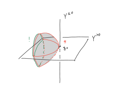
Figure 1. Structure of $k_{V}$ where $V=B^{\prime}\cap\{F\geq 0\}$.

By adjunction, the $!$-restriction along $i:Y^{>0}\to Y$ is internally corepresented

(2.11) $$i^{!}(-)\simeq\underline{\textup{Hom}}(k_{Y^{>0}},-)$$

by the $!$-extension $k_{Y^{>0}}$ of the constant sheaf on $Y^{>0}$. So the Whittaker functional is corepresented

(2.12) $$\phi_{f,y_{0}}i^{!}(-)=\textup{Hom}(k_{Y^{>0}\cap B\cap\{\operatorname{Re}f\geq 0\}},-)$$

by the $!$-extension $k_{Y^{>0}\cap B\cap\{\operatorname{Re}f\geq 0\}}$ of the constant sheaf on

(2.13) $$Y^{>0}\cap B\cap\{\operatorname{Re}f\geq 0\},$$

where $B\subset Y^{>0}$ is a small open ball around $y_{0}$.

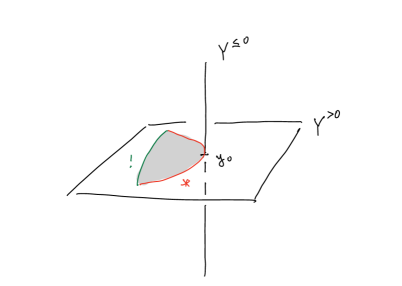
Figure 2. Structure of $k_{Y^{>0}\cap B\cap\{\operatorname{Re}f\geq 0\}}$.

By Lemma 8.4.7 of [KS90], deforming $Y^{>0}$ to a very small closed tube does not change the functor (2.12). More precisely the Whittaker functional

(2.14) $$\phi_{f,y_{0}}i^{!}(-)=\textup{Hom}(k_{W},-)$$

is corepresented by the $!$-extension $k_{W}$ of the constant sheaf on

(2.15) $$W:=B\cap T\cap\{F\geq 0\},$$

where $T\subset Y$ is a very small closed tube around $Y^{>0}$. To apply Lemma 8.4.7 of [KS90] we chose $\varphi$ a distance function from $Y^{>0}$ and used that the sheaf $\underline{\textup{Hom}}(k_{B\cap\{F\geq 0\}},-)$ has compact support. The tube depends on the ball, so $T$ needs to be very small compared to $B$.

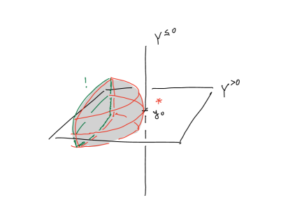
Figure 3. Structure of $k_{W}$ where $W=B\cap T\cap\{F\geq 0\}$.

Finally, taking $B^{\prime}$ small compared to $B$ and $T$ gives an inclusion $V\subset W$ inducing a canonical map $k_{V}\to k_{W}$, and hence a canonical map on corepresented functors

(2.16)

We say a sheaf $\mathcal{F}$ on $Y$ is $\mathbb{C}^{\times}$-monodromic if it is locally constant along each $\mathbb{C}^{\times}$-orbit.

Theorem 2.2.2.

If $\mathcal{F}\in\mathit{Sh}_{\Lambda}(Y)$ is $\mathbb{C}^{\times}$-monodromic (and has singular support in some subanalytic closed conic Lagrangian $\Lambda$) then the map  (2.16) induces an equivalence

(2.17)

Proof.

The kernel of the map (2.16) is corepresented by the $!$-extension $k_{W\setminus V}$ of the constant sheaf on $W\setminus V$. We will show that $W\setminus V$ is foliated by flow lines for the action of $\mathbb{R}^{>0}\subset\mathbb{C}^{\times}$ entering through its $*$-boundary and exiting through its $!$-boundary.

Note the zero locus of the Euler vector field $v$ generating the $\mathbb{R}_{>0}$-action is the fixed locus $Y^{0}$. Since $F|_{Y^{0}\setminus y_{0}}<0$ and $y_{0}$ is not in the closure of $W\setminus V$, the vector field $v$ never vanishes on the closure of $W\setminus V$.

Choose complex coordinate functions $(y^{<0}_{i},y^{0}_{j},y^{>0}_{k})$ so that $\mathbb{C}^{\times}$ acts by $y^{<0}_{i}(z\cdot y)=z^{m_{i}}y^{<0}_{i}(y)$ with negative weights $m_{i}<0$, by $y^{>0}_{k}(z\cdot y)=z^{n_{k}}y^{>0}_{k}(y)$ with positive weights $n_{k}>0$, and fixes the coordinates $y^{0}_{j}(z\cdot y)=y^{0}_{j}(y)$. Consider distance functions (for some metric) in these coordinates

(2.18) $$d_{<0}(y)=\sum|y_{i}^{<0}|^{2},\qquad d_{>0}(y)=\sum|y_{i}^{>0}|^{2},\qquad d_{0}(y)=\sum|y^{0}_{i}|^{2}.$$

Note that acting by $z\in\mathbb{C}^{\times}$ with $|z|>1$ decreases $d_{<0}$ (when non-zero), increases $d_{>0}$ (when non-zero), and fixes $d_{0}$.

Observe we can take $W\setminus V$ to be defined by

(2.19) $$F\geq 0,\qquad a\leq d_{>0}<b,\qquad d_{0}\leq c,\qquad d_{<0}\leq d$$

where $c,d>0$ are small compared with $b>0$, and $a>0$ is small compared with $c,d$. The boundary components of $W\setminus V$ are given by the equations

(2.20) $$F=0,\qquad d_{>0}=a,\qquad d_{>0}=b,\qquad d_{<0}=c,\qquad d_{0}=d.$$

Observe that $k_{W\setminus V}$ is a $!$-extension along the $d_{>0}=b$ boundary component and a $*$-extension along all the other boundary components. Now we further observe how the Euler vector field $v$ interacts with the boundary components:

• $v$ is tangent to $\{F=0\}\cap Y^{>0}=\{\operatorname{Re}f=0\}$ since if $\operatorname{Re}f(y)=0$, then for $z\in\mathbb{R}^{>0}$, we have $\operatorname{Re}f(z\cdot y)=\operatorname{Re}(z^{n}f(y))=z^{n}\operatorname{Re}f(y)=0$. (Here we use $f:Y^{>0}\to\mathbb{C}$ is $\mathbb{C}^{\times}$-equivariant for a linear $\mathbb{C}^{\times}$-action on the target $\mathbb{C}$ by some weight $n$.)

• $v$ is inward pointing on the rest of the face $F=0$ away from $Y^{>0}$ since by assumption $F|_{Y^{\leq 0}\setminus y_{0}}>0$.

• $v$ is inward pointing along the faces $d_{>0}=a$ and $d_{<0}=c$ and outward pointing along the face $d_{>0}=b$ because acting by $z\in\mathbb{R}^{>0}$, with $z>1$, decreases $d_{<0}$ and increases $d_{>0}$ where they are non-zero.

• $v$ is tangent to the face $d_{0}=d$ because acting by $z\in\mathbb{R}^{>0}$ fixes $d_{0}$.

We conclude $W\setminus V$ is foliated by flow segments for the action of $\mathbb{R}^{>0}\subset\mathbb{C}^{\times}$ entering through its $*$-boundary and exiting through its $!$-boundary. The kernel of $\phi_{f,y_{0}}i^{!}\mathcal{F}\to\phi_{F,y_{0}}\mathcal{F}$ is global sections of the sheaf $\underline{\textup{Hom}}(k_{W\setminus V},\mathcal{F})$. If $\mathcal{F}$ is $\mathbb{C}^{\times}$-monodromic, then the pushforward of $\underline{\textup{Hom}}(k_{W\setminus V},\mathcal{F})$ to the quotient $Y/\mathbb{R}_{>0}$ is already zero, so its global sections are zero. ∎

2.3. Calculation of the shift

As in Section 2.2, let $Y^{>0}$ be the attracting locus to $y_{0}$ and let $Y^{\leq 0}$ be the repelling locus. In applying Theorem 2.2.2, we want to be able to interpret the vanishing cycles $\phi_{F,y_{0}}$ as a microstalk. To this end, we want to be able to choose a real valued function $F$ on $Y$ extending $f$ on $Y^{>0}$ not only satisfying the required properties from Section 2.2 but also such that the graph of the differential $\Gamma_{dF}$ intersects the singular support transversely at a smooth point.

Proposition 2.3.1.

Assume that the shifted conormal $T^{*}_{Y^{>0}}Y+df$ intersects $\Lambda$ cleanly and the dimension of the clean intersection is bounded above by

(2.21) $$\dim(\Lambda\cap(T^{*}_{Y^{>0}}Y+df))\leq\dim Y^{\leq 0}.$$

Then there exists a function $F:Y\rightarrow\mathbb{R}$ satisfying the following properties

• $F|_{Y^{>0}}=\operatorname{Re}f$,

• $F_{Y^{\leq 0}\setminus y_{0}}<0$,

• the graph $\Gamma_{dF}$ intersects $\Lambda$ transversely at a smooth point.

Proof.

The first condition is equivalent to $(\Gamma_{dF})|_{Y^{>0}}\subset(T^{*}_{Y^{>0}}Y+d\operatorname{Re}f)$. In other words, above $Y^{>0}$ the graph $\Gamma_{dF}$ restricts to a section of the shifted conormal. By (2.21) it is possible to choose a section $(\Gamma_{dF})|_{Y^{>0}}$ of the shifted conormal intersecting $\Lambda\cap(T^{*}_{Y^{>0}}Y+df)$ transversely. The remaining two conditions imply that $dF(y_{0})=df(y_{0})$ and only depend on $T_{df(y_{0})}\Gamma_{dF}$ the tangent space to the graph. Therefore it is a matter of linear algebra to extend $(\Gamma_{dF})|_{Y^{>0}}$ to a transverse maximally negative definite section $\Gamma_{dF}$ over all of $Y$. Consider the space of graphical Lagrangian subspaces of $T_{df(y_{0})}T^{*}Y$ containing $(\Gamma_{dF})|_{Y^{>0}}$. A generic such subspace will satisfy the third transversality condition. The second condition is open and using local coordinates nonempty. Therefore the desired $F$ exists. ∎

Choose a function $F:Y\rightarrow\mathbb{R}$ as in Proposition 2.3.1 so that $\phi_{F,y_{0}}$ calculates the microstalk at the intersection point $\Lambda\cap\Gamma_{dF}$.

Remark 2.3.2 (Real versus holomorphic tangent bundles).

For a holomorphic function $f$ on $Y^{>0}$ the differential $df(y)\in(T_{y}^{*}Y^{>0}\otimes_{\mathbb{R}}\mathbb{C})^{1,0}$ lies in the holomorphic tangent bundle. Alternatively, we could take the differential of the real part $(d\operatorname{Re}f)(y)\in T_{y}^{*}Y^{>0}$. We identify the holomorphic tangent bundle with the tangent bundle of the underlying real manifold by

(2.22)

where the second map is dual to the inclusion $T_{y}Y^{>0}\hookrightarrow T_{y}Y^{>0}\otimes_{\mathbb{R}}\mathbb{C}.$ Therefore we let $T^{*}Y^{>0}$ also denote the holomorphic tangent bundle. For a holomorphic function $f$, we are free to confuse $df(y)$ with $d\operatorname{Re}f(y)$. Moreover, the two shifted conormal bundles $T^{*}_{Y^{>0}}Y+df$ and $T^{*}_{Y^{>0}}Y+d\operatorname{Re}f$ are identified inside $T^{*}Y$.

Moreover $\phi_{F,y_{0}}$ is exact up to a shift by the Maslov index of three Lagrangians

(2.23) $$\lambda_{\mathit{vert}}:=T_{df(y_{0})}T^{*}_{y_{0}}Y,\quad\lambda:=T_{df(y_{0})}\Lambda,\quad\lambda_{F}:=T_{df(y_{0})}\Gamma_{dF}$$

inside the symplectic vector space $T_{df(y_{0})}T^{*}Y$.

Proposition 2.3.3.

Assume that $\Lambda\subset T^{*}Y$ is a closed conic complex subanalytic Lagrangian preserved by the hyperbolic action, $F|_{Y^{>0}}=\operatorname{Re}f$ is the real part of a $\mathbb{G}_{m}$-equivariant holomorphic function, on the repelling locus $F|_{Y^{\leq 0}}$ is maximized at $y_{0}$ and the graph of $dF$ intersects $\Lambda$ transversely at a smooth point. Then the vanishing cycles functor

(2.24)

is exact and commutes with the Verdier duality functor $D$.

Proof.

Vanishing cycles for $F$ at $y_{0}$ is exact after a shift by $\textup{ind}(\lambda_{\mathit{vert}},\lambda,\lambda_{F})/2$, the Maslov index of three Lagrangrians defined in (2.23). This follows by Proposition 7.5.3 of [KS90] and the fact that vanishing cycles for a holomorphic function is exact. The index is calculated in Proposition 2.3.6. Since $\Gamma_{dF}$ intersects $\Lambda$ transversely at a smooth point, (2.24) is a microstalk and therefore commutes with Verdier duality by the following Proposition 2.3.4. ∎

Below we prove the standard fact that in the complex analytic setting, microstalk at a smooth point of the singular support commutes with Verdier duality.

Proposition 2.3.4.

If $\Lambda\subset T^{*}Y$ is a complex subanalytic closed conic Lagrangian then microstalk at a smooth point $\xi_{0}\in\Lambda$ commutes with Verdier duality.

Proof.

The microstalk category $\mathit{Sh}_{\Lambda}(Y)_{\xi_{0}}$ is defined in Section 6.1 of [KS90] by localizing with respect to all sheaves singular supported away from $\xi_{0}$. Moreover $\mathit{Sh}_{\Lambda}(Y)_{\xi_{0}}$ is invariant under contact transformations by Corollary 7.2.2 of [KS90]. Since $\xi_{0}$ is a smooth point of $\Lambda$, the proof of Corollary 1.6.4 of [KK81] gives a contact transformation taking a neighborhood of $\xi_{0}$ in $\Lambda$ to a neighborhood in the conormal bundle to a smooth hypersurface. Therefore $\mathit{Sh}_{\Lambda}(Y)_{\xi_{0}}=\textup{Vect}$ by Proposition 6.6.1 of [KS90]. Since $\Lambda$ is complex subanalytic, Verdier duality on $\mathit{Sh}_{\Lambda}(Y)_{\xi_{0}}$ preserves singular support, see Exercise V.13 of [KS90]. Both the microstalk at $\xi_{0}$ and its conjugate by Verdier duality vanish on sheaves singular supported away from $\xi_{0}$, so they both factor through the microstalk category $\mathit{Sh}_{\Lambda}(Y)_{\xi_{0}}\simeq\textup{Vect}$ and therefore coincide. ∎

If $\Lambda$ is a smooth closed conic Lagrangian then it is the conormal to a smooth submanifold $\Lambda=T^{*}_{Z}Y$ ([KS90] Exercise A.2) and the Maslov index of (2.23) is the signature of the Hessian of $F$ restricted to $Z$. This is not the case in our application. Although the global nilpotent cone is smooth near $df(y_{0})$, it is not smooth near $y_{0}$ in the zero section. But the Maslov index only depends on the tangent space to $\Lambda$ at $df(y_{0})$. So to compute the index we will choose a submanifold $Z$ whose conormal bundle is tangent to $\Lambda$ at $df(y_{0})$ and then study the Hessian of $F|_{Z}$.

Proposition 2.3.5.

Let $\Lambda\subset T^{*}Y$ be a closed conic Lagrangian that is smooth near $df(y_{0})$ and preserved by the hyperbolic $\mathbb{G}_{m}$-action. Set $\lambda=T_{df(y_{0})}\Lambda$. Then there exists a hyperbolic $\mathbb{G}_{m}$-stable submanifold $Z\subset Y$ such that the tangent spaces coincide:

(2.25) $$T_{df(y_{0})}T_{Z}^{*}Y=\lambda.$$

Proof.

If $df(y_{0})=0$ is in the zero section, then by smoothness $\Lambda=T_{Z}^{*}Y$ is conormal to a smooth $\mathbb{G}_{m}$-equivariant submanifold $Z$, above a neighborhood of $y_{0}\in Y$.

If $df(y_{0})\neq 0$ is not in the zero section, then the tangent space to the conormal $T_{df(y_{0})}T_{Z}^{*}Y$ is determined by the tangent space $T_{y_{0}}Z$ plus the quadratic order behavior of $Z$ in the $df(y_{0})$ codirection. Set $\rho=\lambda\cap\lambda_{\mathit{vert}}$ regarded as a subspace of the vertical $\lambda_{\mathit{vert}}=T^{*}_{y_{0}}Y$. (Note $\rho$ contains at least the tangent to the line through $df(y_{0})$.) There are two different things that we could mean by the orthogonal of $\rho$: its symplectic orthogonal $\rho_{\perp}\subset T_{df(y_{0})}T^{*}Y$, or its orthogonal under duality $\rho^{\perp}\subset T_{y_{0}}Y$.

Let $\mathsf{L}$ be the set of:

• Lagrangians $\lambda^{\prime}\subset T_{df(y_{0})}T^{*}Y$ with vertical component $\lambda^{\prime}\cap\lambda_{\mathit{vert}}=\rho$,

• or equivalently Lagrangians $\lambda^{\prime}/\rho\subset\rho_{\perp}/\rho$ transverse to the vertical fiber.

Then $\mathsf{L}$ is a torsor for the vector space of quadratic forms on $\rho^{\perp}$. Indeed if we choose a reference Lagrangian $\lambda_{0}\in\mathsf{L}$ then we can identify $\rho_{\perp}/\rho=T^{*}\rho^{\perp}$ using $\lambda_{0}/\rho$ as the zero section. A Lagrangian in $T^{*}\rho^{\perp}$ transverse to the vertical fiber is the graph of a quadratic form on $\rho^{\perp}$.

Let $\mathsf{G}$ be the set of germs of submanifolds $Z^{\prime}\subset Y$ with tangent space $T_{y_{0}}Z^{\prime}=\rho^{\perp}$ up to quadratic order equivalence. This is a torsor for the space of quadratic forms from $\rho^{\perp}$ to the normal space. Indeed if we choose a reference $[Z_{0}]\in\mathsf{G}$ then quadratic germs in $\mathsf{G}$ can be identified with the graphs of quadratic forms $T_{y_{0}}Z_{0}\rightarrow(T_{Z_{0}}Y)_{y_{0}}$.

Taking the tangent space to the conormal bundle gives a map

(2.26)

There are two commuting $\mathbb{G}_{m}$ actions on $T^{*}Y$: the cotangent fiber scaling action and the Hamiltonian action induced by the hyperbolic action on $Y$. Neither action fixes the point $df(y_{0})$. However there is some combination of the two actions which fixes $df(y_{0})$ and therefore acts linearly on $T_{df(y_{0})}T^{*}Y$. This is because $y_{0}$ is a fixed point and $f:Y^{>0}\rightarrow\mathbb{C}$ is $\mathbb{G}_{m}$-equivariant where $\mathbb{G}_{m}$ acts on $\mathbb{C}$ with some weight $n$. Therefore we get a $\mathbb{G}_{m}$-action on $\mathsf{L}$ for which $\mathsf{G}\rightarrow\mathsf{L}$ is equivariant.

First, choose any $\mathbb{G}_{m}$-stable germ $[Z_{0}]\in\mathsf{G}$. This gives identifications $\mathsf{L}\simeq\textup{Hom}(\textup{Sym}^{2}(T_{y_{0}}Z_{0}),\mathbb{C})$ and $\mathsf{G}\simeq\textup{Hom}(\textup{Sym}^{2}(T_{y_{0}}Z_{0}),(T_{Y_{0}}Y)_{y_{0}})$ compatibly with all $\mathbb{G}_{m}$-actions (in particular the weight $n$ action on $\mathbb{C}$). Then (2.26) is identified with

(2.27)

given by composition with $df:(T_{Z_{0}}Y)_{y_{0}}\rightarrow\mathbb{C}$.

Since $\Lambda\subset T^{*}Y$ is preserved by both $\mathbb{G}_{m}$-actions, its tangent space $\lambda$ is preserved by the combined action on $T_{df(y_{0})}T^{*}Y$. Therefore the associated quadratic form $\textup{Sym}^{2}(T_{y_{0}}Z_{0})\rightarrow\mathbb{C}$ is $\mathbb{G}_{m}$-equivariant. Lift it along (2.27) to a $\mathbb{G}_{m}$-equivariant quadratic form $\textup{Sym}^{2}(T_{y_{0}}Z_{0})\rightarrow(T_{Z_{0}}Y)_{y_{0}}$. This gives a $\mathbb{G}_{m}$-equivariant germ $[Z]\in\mathsf{G}$ whose conormal is $\lambda$.

It just remains to lift the $\mathbb{G}_{m}$-stable germ $[Z]\in\mathsf{G}$ to a genuine $\mathbb{G}_{m}$-stable submanifold. Suppose $[Z]$ is cut out from $\textup{Spec }(\mathcal{O}_{Y,y_{0}}/\mathfrak{m}^{3})$ by polynomials $\overline{f}_{1},\dots\overline{f}_{d}\in\mathcal{O}_{Y,y_{0}}/\mathfrak{m}^{3}$ that are $\mathbb{G}_{m}$-eigenvectors and whose differentials at $y_{0}$ are linearly independent. Lift them to polynomials $f_{1},\dots f_{d}$ in $\mathcal{O}_{Y,y_{0}}$ that are $\mathbb{G}_{m}$-eigenvectors. Then the lifts $f_{1},\dots f_{d}$ cut out a $\mathbb{G}_{m}$-stable submanifold $Z$ in a neighborhood of $y_{0}$ satisfying the desired $T_{df(y_{0})}T_{Z}^{*}Y=\lambda$. ∎

Now we are ready to replace $\Lambda$ by a conormal bundle and calculate the Maslov index.

Proposition 2.3.6.

Under the same assumptions as Proposition 2.3.3, the Maslov half-index of the three Lagrangian subspaces (2.23) inside $T_{df(y_{0})}T^{*}Y$ is

(2.28) $$\textup{ind}(\lambda_{\mathit{vert}},\lambda,\lambda_{F})/2=\dim Y^{\leq 0}-\dim(\Lambda\cap(T^{*}_{Y^{>0}}Y+df)).$$

Proof.

Use Proposition 2.3.5 to choose a $\mathbb{G}_{m}$-stable submanifold $Z$ such that $T_{df(y_{0})}T^{*}_{Z}Y=\lambda$. Since $df(y_{0})$ vanishes on $T_{y_{0}}Z$, the Hessian of $F|_{Z}$ defines a quadratic form on $T_{y_{0}}Z$ and the sought after index

(2.29) $$\textup{ind}(\lambda_{\mathit{vert}},\lambda,\lambda_{F})/2=-\textup{sgn}(\textup{Hess}F|_{Z})$$

is the negative of the signature of that form. Since the graph $\Gamma_{dF}$ intersects $T_{Z}^{*}Y$ transversely, $\textup{Hess}F|_{Z}$ is nondegenerate. By $\mathbb{G}_{m}$-equivariance $T_{y_{0}}Z=T_{y_{0}}Z^{>0}\oplus T_{y_{0}}Z^{\leq 0}$ splits into attracting and repelling subspaces. By the assumption that $F|_{Z^{\leq 0}-y_{0}}<0$, it follows that the restriction $\textup{Hess}F|_{Z^{\leq 0}}$ is negative definite on the repelling $T_{y_{0}}Z^{\leq 0}$. By the assumption that $F|_{Z^{>0}}$ is holomorphic it follows the restriction $\textup{Hess}F|_{Z^{>0}}$ to $T_{y_{0}}Z^{>0}$ has signature $0$.

Therefore the number of positive eigenvalues of $\textup{Hess}F|_{Z}$ equals the number of positive eigenvalues of $\textup{Hess}F|_{Z^{>0}}$ which is

(2.30) $$(\dim Z^{>0}-\textup{null}(\textup{Hess}F|_{Z^{>0}})/2.$$

Here $\textup{null}(\textup{Hess}F|_{Z^{>0}})$ is the multiplicity of 0 as an eigenvalue of the quadratic form. Since $\textup{Hess}F|_{Z}$ is nondegenerate, the remaining eigenvalues are strictly negative. So the index is

(2.31) $$\textup{ind}(\textup{Hess}F|_{Z})/2=-\dim Z^{\leq 0}+\textup{null}(\textup{Hess}F|_{Z^{>0}}).$$

It remains to compare the expression (2.31) with the dimension of the intersection of $\Lambda$ and the shifted conormal. Since the intersection is clean near $df(y_{0})$, we can pass to tangent spaces before calculating the dimension of the intersection.

Let $\lambda_{f}=T_{df(y_{0})}(T^{*}_{Y^{>0}}Y+df)$ be tangent to the shifted conormal, a fourth Lagrangian in $T_{df(y_{0})}T^{*}Y$.

The codifferential of the inclusion of $Z$ maps

(2.32)

and differentiating gives a linear map

(2.33) $$\lx@xy@svg{\hbox{\raise 0.0pt\hbox{\kern 38.27777pt\hbox{\ignorespaces\ignorespaces\ignorespaces\hbox{\vtop{\kern 0.0pt\offinterlineskip\halign{\entry@#!@&&\entry@@#!@\cr&\crcr}}}\ignorespaces{\hbox{\kern-38.27777pt\raise 0.0pt\hbox{\hbox{\kern 0.0pt\raise 0.0pt\hbox{\hbox{\kern 3.0pt\raise 0.0pt\hbox{$\textstyle{\pi:T_{df(y_{0})}(T^{*}Y|_{Z})\ignorespaces\ignorespaces\ignorespaces\ignorespaces}$}}}}}}}\ignorespaces\ignorespaces\ignorespaces\ignorespaces{}{\hbox{\lx@xy@droprule}}\ignorespaces{\hbox{\kern 62.74443pt\raise 0.0pt\hbox{\hbox{\kern 0.0pt\raise 0.0pt\hbox{\lx@xy@tip{1}\lx@xy@tip{-1}}}}}}{\hbox{\lx@xy@droprule}}{\hbox{\lx@xy@droprule}}{\hbox{\kern 62.74443pt\raise 0.0pt\hbox{\hbox{\kern 0.0pt\raise 0.0pt\hbox{\hbox{\kern 3.0pt\raise 0.0pt\hbox{$\textstyle{T_{y_{0}}T^{*}Z}$}}}}}}}\ignorespaces}}}}\ignorespaces. \textstyle{\pi:T_{df(y_{0})}(T^{*}Y|_{Z})\ignorespaces\ignorespaces\ignorespaces\ignorespaces} \textstyle{T_{y_{0}}T^{*}Z} \textstyle{\pi:T_{df(y_{0})}(T^{*}Y|_{Z})\ignorespaces\ignorespaces\ignorespaces\ignorespaces} \textstyle{T_{y_{0}}T^{*}Z}$$

Since $\lambda\subset T_{df(y_{0})}(T^{*}Y|_{Z})$, we can calculate the dimension of $\lambda\cap\lambda_{f}$ from the rank and nullity of $\pi$ restricted to $\lambda\cap\lambda_{f}$.

By $\mathbb{G}_{m}$-invariance, $Z$ intersects $Y^{>0}$ cleanly and so the inclusion $T_{df(y_{0})}((T^{*}_{Y^{>0}}Y+df)|_{Z})\subset\lambda_{f}|_{T_{y_{0}}Z}$ is an equality. In other words, for the shifted conormal, passing to tangent spaces commutes with restriction to $Z$. Moreover the coderivative (2.32) maps $(T^{*}_{Y^{>0}}Y+df)|_{Z}$ smoothly to the shifted conormal bundle $T^{*}_{Z^{>0}}Z+df|_{Z^{>0}}$. By smoothness, passing to tangent spaces commutes with taking the image along $di^{*}$ and $\pi$. Therefore,

(2.34) $$\begin{split}\pi(\lambda_{f}|_{T_{y_{0}}Z})&=T_{y_{0}}(T^{*}_{Z^{>0}}Z+df|_{Z^{>0}})=T_{y_{0}}T^{*}_{Z^{>0}}Z+\Gamma_{\textup{Hess}F|_{Z^{>0}}}\\ &=\{v\in T_{y_{0}}Z^{>0},\xi\in T_{y_{0}}^{*}Z\text{ such that }\xi(w)=(\textup{Hess}F)(v,w)\text{ for }w\in T_{y_{0}}Z^{>0}\},\end{split}$$

is the conormal to $T_{y_{0}}Z^{>0}\subset T_{y_{0}}Z$ shifted by the graph of the Hessian of $F|_{Z^{>0}}$.

Moreover, $\lambda=\pi^{-1}(\xi=0)$, for $\xi$ the coordinate on $T_{y_{0}}^{*}Z$, is exactly the preimage in $T_{y_{0}}T^{*}Z$ under (2.33) of the zero section $T_{y_{0}}Z$. Therefore

(2.35) $$\pi(\lambda\cap\lambda_{f})=T_{y_{0}}Z\cap\pi(\lambda_{f}|_{T_{y_{0}}Z})$$

is the nullspace of $\textup{Hess}F|_{Z^{>0}}$ inside the zero section. So the dimension of $\pi(\lambda\cap\lambda_{f})$ is

(2.36) $$\textup{rank}\ (\pi|_{\lambda\cap\lambda_{f}})=\textup{null}(\textup{Hess}F|_{Z^{>0}}).$$

The kernel of $\pi|_{\lambda\cap\lambda_{f}}$ is $((T_{y_{0}}Z)^{\perp}\cap(T_{y_{0}}Y^{>0})^{\perp})$ inside the vertical $T^{*}_{y_{0}}Y\subset T_{df(y_{0})}T^{*}Y$ of dimension

(2.37) $$\textup{null}(\pi|_{\lambda\cap\lambda_{f}})=\dim Y^{\leq 0}-\dim Z^{\leq 0}.$$

Combining (2.36) and (2.37) gives

(2.38) $$\dim(\lambda\cap\lambda_{f})=\dim Y^{\leq 0}-\dim Z^{\leq 0}+\textup{null}(\textup{Hess}F|_{Z^{>0}})$$

which together with (2.31) gives the desired formula (2.28) for the shift. ∎

Example 2.3.7.

Let $Y=\mathbb{A}^{2}$ with hyperbolic action $z\cdot(x,y)=(zx,z^{-1}y)$. So $i$ is the inclusion of $Y^{>0}=\{y=0\}$.

The Whittaker functional of the skyscraper sheaf $k_{0}$ is

(2.39) $$\phi_{x,0}i^{!}k_{0}=\phi_{x,0}k_{0}=k.$$

The singular support $\Lambda=T_{0}^{*}\mathbb{A}^{2}$ of the skyscraper intersects the shifted conormal bundle $(T_{Y^{>0}}\mathbb{A}^{2}+dx)$ in the one dimensional space $(T_{y=0}^{*}\mathbb{A}^{2})_{0}+dx$ so

(2.40) $$\dim Y^{\leq 0}-\dim(T_{0}^{*}\mathbb{A}^{2}\cap(T_{Y^{>0}}^{*}\mathbb{A}^{2}+dx))=0$$

and there is no shift.

The Whittaker functional of the perverse sheaf $k_{x=0}[1]$ is

(2.41) $$\phi_{x,0}i^{!}k_{x=0}[1]=\phi_{x,0}k_{x=0}[-1]=k[-1].$$

The resulting vector space becomes perverse after shifting by

(2.42) $$\dim Y^{\leq 0}-\dim(T^{*}_{x=0}\mathbb{A}^{2}\cap(T_{Y^{>0}}^{*}\mathbb{A}^{2}+dx))=1$$

because the singular support $\Lambda=T^{*}_{x=0}\mathbb{A}^{2}$ intersects the shifted conormal bundle in a single point.

3. Application to automorphic sheaves

Let $X$ be a smooth connected projective complex curve with canonical bundle denoted by $\omega$. Let $G$ be a complex reductive group with Borel subgroup $B\subset G$ with unipotent radical $N=[B,B]$ and universal Cartan $T=B/N$. For concreteness, we will fix a splitting $T\subset B$.

3.1. The Whittaker functional under uniformization

Let $\rho^{\vee}$ be half the sum of the positive coroots. Choose a square root $\omega^{1/2}$ of the canonical bundle and consider the $T$-bundle $\rho^{\vee}(\omega):=2\rho^{\vee}(\omega^{1/2})$. Its key property is that for every simple root $\alpha$, the associated line bundle $\rho^{\vee}(\omega)\times_{T}\mathbb{C}_{\alpha}=\omega^{\langle\rho^{\vee},\alpha\rangle}=\omega$ is canonical. Let $\textup{Bun}_{N}^{\omega}(X)$ be the moduli of $B$-bundles on $X$ whose underlying $T$-bundle is $\rho^{\vee}(\omega)$. Thus $\textup{Bun}_{N}^{\omega}(X)$ classifies maps $X\to\textup{pt}/B$ such that the composition with $\textup{pt}/B\to\textup{pt}/T$ classifies the $T$-bundle $\rho^{\vee}(\omega)$. Such maps factor through the classifying space of $B\times_{T}2\rho^{\vee}(\mathbb{G}_{m})\simeq N\rtimes\mathbb{G}_{m}$ as in the diagram:

(3.1)

So alternatively $\textup{Bun}_{N}^{\omega}(X)$ is represented by maps to $\textup{pt}/(N\rtimes\mathbb{G}_{m})$ such that the composition to $\textup{pt}/\mathbb{G}_{m}$ classifies $\omega^{1/2}$.

The semidirect product $N\rtimes\mathbb{G}_{m}$ mentioned above is formed by letting $z\in\mathbb{G}_{m}$ act on $N$ by conjugation by $2\rho^{\vee}(z)\in T$. In other words, $N\rtimes\mathbb{G}_{m}\subset B$ is the subgroup of the Borel generated by $N$ and $2\rho^{\vee}(\mathbb{G}_{m})$. Consider the action of $N\rtimes\mathbb{G}_{m}$ on $\mathfrak{n}^{*}$ by

(3.2) $$z\cdot X=\textup{Ad}_{2\rho^{\vee}(z)}(z^{2}X),$$

the product of scaling and the adjoint $T$-action.

Proposition 3.1.1.

The cotangent bundle $T^{*}\textup{Bun}_{N}^{\omega}(X)$ is represented by maps $X\to\mathfrak{n}^{*}/(N\rtimes\mathbb{G}_{m})$, where we quotient by the (3.2) action, such that the composition $X\to\textup{pt}/\mathbb{G}_{m}$ classifies the line bundle $\omega^{1/2}$.

Proof.

By definition $\textup{Bun}_{N}^{\omega}(X)$ is a fiber of the smooth (but not representable) map $p:\textup{Bun}_{B}(X)\to\textup{Bun}_{T}(X)$. The relative tangent complex of $p$ is $(\pi_{*}\mathfrak{b}_{F^{\textup{univ}}}[1]\to\pi_{*}\mathfrak{t}_{F^{\textup{univ}}})\simeq\pi_{*}\mathfrak{n}_{F^{\textup{univ}}}[1]$ given by pushing forward vector bundles associated to the universal $B$-bundle $F^{\textup{univ}}$ along $\pi:X\times\textup{Bun}_{B}(X)\to\textup{Bun}_{B}(X)$. The tangent complex of $\textup{Bun}_{N}^{\omega}(X)$ is the restriction $\pi_{*}\mathfrak{n}_{F^{\textup{univ}}}|_{\textup{Bun}_{N}^{\omega}(X)}[1]$. Taking the stalk at a point $F\in\textup{Bun}_{N}^{\omega}(X)$ gives the tangent space $T_{F}\textup{Bun}_{N}^{\omega}(X)=H^{1}(\mathfrak{n}_{F})$. By Serre duality the cotangent space is

(3.3) $$T^{*}_{F}\textup{Bun}_{N}^{\omega}(X)=H^{0}(\mathfrak{n}^{*}_{F}\otimes\omega).$$

Here $\mathfrak{n}^{*}_{F}$ is the vector bundle obtained from $F$ via the adjoint action of $B$ on $\mathfrak{n}^{*}$. Whereas $\mathfrak{n}^{*}_{F}\otimes\omega$ is obtained from $F$ via $N\rtimes\mathbb{G}_{m}$ acting on $\mathfrak{n}^{*}$ by (3.2).

So giving a cotangent vector in $T_{F}^{*}\textup{Bun}_{N}^{\omega}(X)$ is equivalent to lifting the classifying map $X\to\textup{pt}/(N\rtimes\mathbb{G}_{m})$ of the bundle $F$ to a map $X\to\mathfrak{n}^{*}/(N\rtimes\mathbb{G}_{m})$. It was important that we modified the adjoint $B$-action on $\mathfrak{n}^{*}$ by also scaling so as to incorporate the canonical twist from Serre duality. ∎

Let $f:\textup{Bun}_{N}^{\omega}(X)\to\mathbb{A}^{1}$ be the function given by the sum of the functions

(3.4)

induced by projection onto each simple root space $N\to N/[N,N]\to\mathbb{G}_{a}$. The graph of its differential $\Gamma_{df}\subset T^{*}\textup{Bun}_{N}^{\omega}(X)$ is represented by

(3.5) $$\psi/(N\rtimes\mathbb{G}_{m})\subset\mathfrak{n}^{*}/(N\rtimes\mathbb{G}_{m})$$

where $\psi:\mathfrak{n}\to\mathfrak{n}/[\mathfrak{n},\mathfrak{n}]\to\mathbb{A}^{1}$ is given by summing over the simple root spaces. To see that the expression $\psi/(N\rtimes\mathbb{G}_{m})$ makes sense we need to check that $\psi$ is invariant under the $(N\rtimes\mathbb{G}_{m})$-action. Indeed $\psi$ factors through the abelianization so it is $N$-invariant. Furthermore the adjoint action of $2\rho^{\vee}(z)$ scales the $\alpha_{i}$ simple root space component of $\psi$ by $z^{-\langle 2\rho^{\vee},\alpha_{i}\rangle}=z^{-2}$ cancelling out the $\mathbb{G}_{m}$-scaling action.

Let $\textup{Bun}_{G}(X)$ be the moduli of $G$-bundles on $X$. Recall the cotangent bundle of $\textup{Bun}_{G}(X)$ is the moduli of Higgs bundles

(3.6) $$T^{*}\textup{Bun}_{G}(X)\simeq\{E,\sigma\in H^{0}(\mathfrak{g}^{*}_{E}\otimes\omega)\}$$

classifying maps $X\to\mathfrak{g}^{*}/(G\times\mathbb{G}_{m})$ such that the composition to $\textup{pt}/\mathbb{G}_{m}$ classifies the line bundle $\omega$. The global nilpotent cone $\Lambda\subset T^{*}\textup{Bun}_{G}(X)$ is the moduli of everywhere nilpotent Higgs bundles

(3.7) $$\Lambda=\{E,\sigma\in H^{0}(\mathcal{N}^{*}_{E}\otimes\omega)\}$$

classifying maps $X\to\mathcal{N}^{*}/(G\times\mathbb{G}_{m})$ such that the composition to $\textup{pt}/\mathbb{G}_{m}$ classifies the line bundle $\omega$.

The Whittaker functional

(3.8)

is $!$-pullback along the natural induction map

(3.9)

followed by vanishing cycles for $f$ at the point $\rho^{\vee}(\omega)$. Note one could alternatively take global sections rather than stalk of the vanishing cycles $\phi_{f}$, but this will give the same result by the contraction principle ([KS90] Proposition 3.7.5).

To apply our general results, we would like to locally uniformize the moduli in play and replace them by smooth schemes. To this end, fix a closed point $x\in X$.

First, by taking $n$ large enough, we may factor $i$ through a closed embedding followed by a smooth projection

(3.10)

Here $\textup{Bun}^{\omega}_{G,N}(X,nx)$ is the moduli space of $G$-bundles on $X$ with a $B$-reduction on the $n$th order neighborhood $D_{n}(x)$ whose underlying $T$-bundle is $\rho^{\vee}(\omega)|_{D_{n}(x)}$. The maps factoring $i$ are the natural induction maps; the second is clearly a smooth projection, and we will see momentarily that the first is a closed embedding.

Next, introduce the moduli $\textup{Bun}_{G}^{\omega}(X,nx)$ classifying $G$-bundles on $X$ with a reduction on the $n$th order neighborhood $D_{n}(x)$ to the $\mathbb{G}_{m}$-bundle $\omega^{1/2}$ via the inclusion $2\rho^{\vee}:\mathbb{G}_{m}\to T\subset G$. Form the following induction diagram with a Cartesian square.

(3.11)

Thus $\textup{Bun}_{N}^{\omega}(X,nx)$ classifies objects of $\textup{Bun}_{N}^{\omega}(X)$ with a reduction on $D_{n}(x)$ to the $\mathbb{G}_{m}$-bundle $\omega^{1/2}$ via the inclusion $2\rho^{\vee}:\mathbb{G}_{m}\to T\subset B$.

Take a quasi-compact open substack $U\subset\textup{Bun}_{G}(X)$ containing the image of $\textup{Bun}_{N}^{\omega}(X)$. Then for $n$ sufficiently large, $\textup{Bun}_{G}^{\omega}(X,nx)|_{U}$ is a scheme. Futhermore, at $F\in\textup{Bun}_{N}^{\omega}(X,nx)$, for $n$ sufficiently large, the codifferential

(3.12)

is surjective since $H^{1}(\mathfrak{n}^{\perp}_{F}\otimes\omega(nx))=0$. Moreover, we can choose $n\gg 0$ once and for all uniformly over $\textup{Bun}_{N}^{\omega}(X)$ by quasi-compactness.

Thus for $n$ sufficiently large, since $i^{\prime}$ is a map between smooth schemes with surjective codifferential, it is locally a closed embedding. Applying contraction for the natural $\mathbb{G}_{m}$-action considered below, we see $i^{\prime}$ is in fact a closed embedding. Also, $\textup{Bun}_{N}^{\omega}(X)\to\textup{Bun}^{\omega}_{G,N}(X,nx)$ is a closed embedding because $i^{\prime}$ is a base-change of it via a surjective map.

The cotangent bundle $T^{*}\textup{Bun}_{G}^{\omega}(X,nx)$ classifies data

(3.13) $$T^{*}\textup{Bun}_{G}^{\omega}(X,nx)=\{E,E|_{D_{n}(x)}\simeq G\times_{T}\rho^{\vee}(\omega)|_{D_{n}(x)},\sigma\in H^{0}(\mathfrak{g}^{*}_{E}\otimes\omega(nx))\}.$$

Singular support behaves well under smooth pullback. So if $\mathcal{F}$ is a sheaf on $\textup{Bun}_{G}(X)$ with singular support in the nilpotent cone

(3.14) $$\Lambda=\{E,\sigma\in H^{0}(\mathcal{N}^{*}_{E}\otimes\omega)\}$$

then the singular support of its smooth pullback to $\textup{Bun}_{G}^{\omega}(X,nx)$ lies in

(3.15) $$\Lambda^{\prime}=\Lambda\times_{\textup{Bun}_{G}(X)}\textup{Bun}_{G}^{\omega}(X,nx)=\{E,E|_{D_{n}(x)}\simeq G\times_{T}\rho^{\vee}(\omega)|_{D_{n}(x)},\sigma\in H^{0}(\mathcal{N}^{*}_{E}\otimes\omega)\}.$$

3.2. Hyperbolic symmetry

To apply Theorem 2.2.2, we seek a $\mathbb{G}_{m}$-action for which $i^{\prime}:\textup{Bun}_{N}^{\omega}(X,nx)\to\textup{Bun}_{G}^{\omega}(X,nx)$ is the attracting locus for the bundle $\rho^{\vee}(\omega)$. Let $f^{\prime}:\textup{Bun}_{N}^{\omega}(X,nx)\to\mathbb{A}^{1}$ be the pullback of $f$ to the uniformized moduli space. To apply Theorem 2.2.2 we also need $f^{\prime}$ to be $\mathbb{G}_{m}$-equivariant for some $\mathbb{G}_{m}$ action on $\mathbb{A}^{1}$ (which will turn out to have weight 2).

An automorphism $\alpha\in\textup{Aut}(G)$ induces an automorphism of $\textup{Bun}_{G}(X)$ by twisting the $G$-actions on the underlying bundles. A $G$-bundle $E$ goes to the $G$-bundle $\alpha E$ with the same total space but the old action of $g$ on $E$ is replaced by the new action of $\alpha(g)$ on $\alpha E$. If the automorphism of $G$ is inner, say it is given by conjugation by $h\in G$, then the action on $\textup{Bun}_{G}(X)$ is entirely stacky in the sense that it is trivial on the set of isomorphism classes of points. Indeed the multiplication by $h$ map $h:E\rightarrow\alpha E$ intertwines the original action with the twisted one.

Suppose now that the automorphism $\alpha$ of $G$ is trivial on $T$. Then $\alpha$ also induces an automorphism of $\textup{Bun}_{G}^{\omega}(X,nx)$ with level structure. A $G$-bundle $E$ with canonically twisted trivialization $\phi:E|_{D_{n}(X)}\xrightarrow{\sim}G\times_{T}\rho^{\vee}(\omega)|_{D_{n}(x)}$ goes to the $G$-bundle $\alpha E$ with trivialization

(3.16)

The final map is trivial on the $\rho^{\vee}(\omega)$ factor and is well defined because we assumed that the automorphism $\alpha:G\rightarrow G$ is right $T$-invariant. For example if $\alpha(g)=hgh^{-1}$ is an inner automorphism and $h\in T$, then we get an automorphism of $\textup{Bun}_{G}^{\omega}(X,nx)$ that preserves the underlying bundle and changes the trivialization by conjugation by $h$. In other words $\alpha$ acts along the fibers of $\textup{Bun}_{G}^{\omega}(X,nx)\rightarrow\textup{Bun}_{G}(X)$.

Remark 3.2.1.

For simplicity ignore the canonical twist and suppose that $G$ is semisimple so we have one point uniformization,

(3.17) $$\textup{Bun}_{G}(X,nx)=K_{n}\setminus G(K_{x})/G(X-x).$$

Here $K_{n}\subset G(\mathcal{O}_{x})$ consists of matrices that are the identity to $n$th order. Then the inner automorphism $\alpha(g)=hgh^{-1}$ sends a double coset $K_{n}gG(X-x)$ to $K_{n}hgh^{-1}G(X-x)\simeq K_{n}hgG(X-x)$. Since $h^{-1}$ is a constant function we could absorb it into $G(X-x)$, so alternatively the action is given by changing the trivialization by left multiplication.

Let $z\in\mathbb{G}_{m}$ act on $G$ and $B$ by conjugation by $\rho^{\vee}(z)\in T/Z(G)$ in the torus of the adjoint group. This gives a $\mathbb{G}_{m}$-action on the moduli spaces of bundles for which the natural maps between moduli spaces are equivariant.

Proposition 3.2.2 (4.7 of [DG16]).

Restrict to the connected component of $\textup{Bun}_{B}(X,nx)$ and $\textup{Bun}_{T}(X,nx)$ indexed by the coweight $(2g-2)\rho^{\vee}$. Then for $n$ sufficiently large, $\textup{Bun}_{B}(X,nx)$ is the attracting locus to $\textup{Bun}_{T}(X,nx)$ in an open neighborhood of $\textup{Bun}_{T}(X,nx)$ inside $\textup{Bun}_{G}^{\omega}(X,nx)|_{U}$.

Proof.

The $\mathbb{G}_{m}$-action contracts $\textup{Bun}_{B}(X,nx)$ to $\textup{Bun}_{T}(X,nx)$ because $\rho^{\vee}(\mathbb{G}_{m})$ contracts $B$ to $T$. Indeed if $F$ is a $B$-bundle then acting by $\rho^{\vee}(z)$ gives a bundle with the same total space but $b$ acting by $\rho^{\vee}(z)b\rho^{\vee}(z)^{-1}$. As $z\rightarrow 0$, the conjugate $\rho^{\vee}(z)b\rho^{\vee}(z)^{-1}$ approaches an element of $T$ so the $B$-bundle approaches one induced from a $T$-bundle.

It remains to check $\textup{Bun}_{B}(X,nx)$ is the full attracting locus in an open neighborhood of $\textup{Bun}_{T}(X,nx)$ inside $\textup{Bun}_{G}^{\omega}(X,nx)$. This is because $p:\textup{Bun}_{B}(X,nx)\to\textup{Bun}_{G}^{\omega}(X,nx)|_{U}$ is a closed embedding (we are implicitly restricting to the connected component containing $\rho^{\vee}(\omega)$ and choosing $n$ large) so $p$ is a closed embedding into the attracting locus. Since $\textup{Bun}_{B}(X,nx)$ is smooth, it suffices to show that $p$ is also an open embedding into a neighborhood of the attracting locus about $\textup{Bun}_{T}(X,nx)$. This follows because the derivative over $L\in\textup{Bun}_{T}(X,nx)$, given by the natural map

(3.18)

maps isomorphically into the non-negative $\mathbb{G}_{m}$-weight spaces. ∎

Since $p:\textup{Bun}_{B}^{\omega}(X,nx)\rightarrow\textup{Bun}_{T}^{\omega}(X,nx)$ is $\mathbb{G}_{m}$-equivariant, the fiber $\textup{Bun}_{N}^{\omega}(X,nx)$ also admits a $\mathbb{G}_{m}$-action. But the action on $\textup{Bun}_{N}^{\omega}(X,nx)$ changes the bundles not just the trivializations because conjugation by $\rho^{\vee}(\mathbb{G}_{m})$ is an outer automorphism of $N$.

Proposition 3.2.3.

The function $f:\textup{Bun}_{N}^{\omega}(X)\rightarrow\mathbb{A}^{1}$ is $\mathbb{G}_{m}$-equivariant.

Proof.

For each positive simple root, projection onto that root space $N\rightarrow\mathbb{G}_{a}$ is $\mathbb{G}_{m}$-equivariant for the $\rho^{\vee}$ action on $N$ and the scaling action on $\mathbb{G}_{a}$. Under uniformization

(3.19) $$\textup{Bun}_{\mathbb{G}_{a}}^{\omega}(X)=\mathcal{O}_{x}dt\setminus K_{x}dt/\omega(X-x)=H^{1}(X,\omega)\times BH^{0}(X,\omega)$$

the scaling action on $\mathbb{G}_{a}$ induces an action that scales the gluing data in $K_{x}dt$. The residue map $K_{x}dt\rightarrow\mathbb{A}^{1}$ descends to the map $\textup{Bun}_{\mathbb{G}_{a}}^{\omega}(X)\rightarrow\mathbb{A}^{1}$ which is $\mathbb{G}_{m}$-equivariant. Since $f$ is defined as the sum over positive simple roots of

(3.20)

it is $\mathbb{G}_{m}$-equivariant. ∎

We are interested in sheaves on $\textup{Bun}_{G}^{\omega}(X,nx)$ pulled back from $\textup{Bun}_{G}(X)$ so they will certainly be $\mathbb{G}_{m}$-equivariant. Alternatively, having singular support in $\Lambda^{\prime}\subset T^{*}\textup{Bun}_{G}^{\omega}(X,nx)$, implies constructibility along the orbits of this $\mathbb{G}_{m}$-action.

Applying theorem 2.2.2 for $Y=\textup{Bun}_{G}^{\omega}(X,nx)$, $y_{0}=\rho^{\vee}(\omega)$ with its canonical level structure, $Y^{>0}=\textup{Bun}_{N}^{\omega}(X,nx)$, and $Y^{\leq 0}=\textup{Bun}_{B^{-}}(X,nx)$ gives the following. Let $f^{\prime}$ be the pullback to $\textup{Bun}_{N}^{\omega}(X,nx)$ of $f$ .

Proposition 3.2.4.

There is an isomorphism of functors

(3.21) $$\phi_{f^{\prime},\rho^{\vee}(\omega)}i^{\prime!}=\phi_{F,\rho^{\vee}(\omega)}:\mathit{Sh}_{\Lambda^{\prime}}(\textup{Bun}_{G}^{\omega}(X,nx))\to\textup{Vect}.$$

Here $F$ is a real valued extension of $f^{\prime}$ as in theorem 2.2.2 satisfying $F|_{\textup{Bun}_{N}^{\omega}(X,nx)}=\operatorname{Re}f^{\prime}$ and $F|_{\textup{Bun}_{B^{-}}^{\omega}(X,nx)-\rho^{\vee}(\omega)}<0$.

Vanishing cycles commutes with smooth pullback, so $\phi_{f,\rho^{\vee}(\omega)}i^{!}$ and $\phi_{f^{\prime},\rho^{\vee}(\omega)}i^{\prime!}$ agree up to a shift

(3.22) $$\phi_{f,\rho^{\vee}(\omega)}i^{!}[2n\dim N]\simeq\phi_{f^{\prime},\rho^{\vee}(\omega)}i^{\prime!}\pi^{!}.$$

Therefore we are free to pull everything back to $\textup{Bun}_{G}^{\omega}(X,nx)$ where $F$ is defined. Note that $!$-pullback along

(3.23)

is not exact, but by smoothness $\pi^{!}[-n\dim G]$ is.

3.3. Microstalk along the Kostant section

Now we will explain how the shifted conormal is the Kostant section of the Hitchin fibration and therefore intersects the global nilpotent cone transversely in a single smooth point.

Proposition 3.3.1.

Inside $T^{*}\textup{Bun}_{G}(X)$ the shifted conormal bundle $T^{*}_{\textup{Bun}_{N}^{\omega}(X)}\textup{Bun}_{G}(X)+df$ intersects the global nilpotent cone $\Lambda$ transversely at a smooth point.

Proof.

The shifted conormal bundle consists of cotangent vectors $X\to\mathfrak{g}^{*}/(N\rtimes\mathbb{G}_{m})$ in $(T^{*}\textup{Bun}_{G}(X))|_{\textup{Bun}_{N}^{\omega}(X)}$ such that the composition

(3.24)

lands in $\psi/(N\rtimes\mathbb{G}_{m})$. Therefore $T^{*}_{\textup{Bun}_{N}^{\omega}(X)}\textup{Bun}_{G}+df$ is represented by the Kostant section

(3.25)

We used the homomorphism

(3.26) $$N\rtimes\mathbb{G}_{m}\to G\times\mathbb{G}_{m},\qquad n\rtimes z\mapsto(n\cdot 2\rho^{\vee}(z),z^{2}).$$

This is a section of the characteristic polynomial map $\mathfrak{g}^{*}/(G\times\mathbb{G}_{m})\to\mathfrak{c}^{*}/\mathbb{G}_{m}$ which represents the Hitchin map

(3.27)

Let $T^{*}\textup{Bun}_{G}(X)^{\textup{reg}}$ be the regular locus, represented by $\mathfrak{g}^{*,\textup{reg}}/(G\times\mathbb{G}_{m})\subset\mathfrak{g}^{*}/(G\times\mathbb{G}_{m})$. It is an open substack of $T^{*}\textup{Bun}_{G}(X)$ because $\mathfrak{g}^{*,\textup{reg}}\subset\mathfrak{g}^{*}$ is open and $X$ is proper. The Hitchin fibration $h$ is smooth after restricting to this regular locus. Since $\psi+\mathfrak{n}^{\perp}\subset\mathfrak{g}^{*,\textup{reg}}$ consists of regular elements the Kostant section is contained in $T^{*}\textup{Bun}_{G}(X)^{\textup{reg}}$. After restricting to $T^{*}\textup{Bun}_{G}(X)^{\textup{reg}}$, the Kostant section is a section of a smooth projection so intersects every fiber, in particular the global nilpotent cone, transversely at a smooth point. ∎

Since $i$ is not a closed embedding we factored it through $\textup{Bun}_{N}^{\omega}(X)\rightarrow\textup{Bun}_{G,N}^{\omega}(X,nx)$.

Proposition 3.3.2.

Inside $T^{*}\textup{Bun}_{G,N}^{\omega}(X,nx)$, the shifted conormal bundle

(3.28) $$\Lambda_{f}^{\prime\prime}:=df+T^{*}_{\textup{Bun}_{N}^{\omega}(X)}\textup{Bun}^{\omega}_{G,N}(X,nx)$$

intersects the global nilpotent cone

(3.29) $$\Lambda^{\prime\prime}=\Lambda\times_{\textup{Bun}_{G}(X)}\textup{Bun}^{\omega}_{G,N}(X,nx)$$

transversely at a single smooth point.

Proof.

The nilpotent cone $\Lambda^{\prime\prime}$ is contained inside

(3.30) $$\mu^{-1}(0)/N:=T^{*}\textup{Bun}_{G}(X)\times_{\textup{Bun}_{G}(X)}\textup{Bun}^{\omega}_{G,N}(X,nx).$$

Whereas we claim that the shifted conormal $\Lambda_{f}^{\prime\prime}$ intersects $\mu^{-1}(0)/N$ transversely. By the previous Proposition 3.3.1,

(3.31) $$\Lambda_{f}^{\prime\prime}\cap(\mu^{-1}(0)/N)=df+T^{*}_{\textup{Bun}_{N}^{\omega}(X)}\textup{Bun}_{G}(X)$$

intersects $\Lambda^{\prime\prime}$ transversely inside $\mu^{-1}(0)/N$ at a single smooth point of $\Lambda^{\prime\prime}$. Therefore $\Lambda_{f}^{\prime\prime}$ and $\Lambda^{\prime\prime}$ intersect transversely as desired.

To see the claim that $\Lambda_{f}^{\prime\prime}$ and $\mu^{-1}(0)/N$ intersect transversely we need to check that their tangent spaces at $df(\rho^{\vee}(\omega))$ together span the whole $T_{df(\rho^{\vee}(\omega))}T^{*}\textup{Bun}_{G,N}^{\omega}(X,nx)$. Projecting onto the horizontal directions, $T_{df(\rho^{\vee}(\omega))}T^{*}\textup{Bun}_{G,N}^{\omega}(X,nx)$ fits into a short exact sequence

(3.32) $$0\rightarrow T^{*}_{\rho^{\vee}(\omega)}\textup{Bun}_{G,N}^{\omega}(X,nx)\rightarrow T_{df(\rho^{\vee}(\omega))}T^{*}\textup{Bun}_{G,N}^{\omega}(X,nx)\rightarrow T_{\rho^{\vee}(\omega)}\textup{Bun}_{G,N}^{\omega}(X,nx)\rightarrow 0.$$

The tangent space to $\mu^{-1}(0)/N$ surjects onto $T_{\rho^{\vee}(\omega)}\textup{Bun}_{G,N}^{\omega}(X,nx)$ so it suffices to show that the tangent spaces to $\Lambda_{f}^{\prime\prime}$ and $\mu^{-1}(0)/N$ intersected with the vertical subspace $T^{*}_{\rho^{\vee}(\omega)}\textup{Bun}_{G,N}^{\omega}(X,nx)$ together span the whole $T^{*}_{\rho^{\vee}(\omega)}\textup{Bun}_{G,N}^{\omega}(X,nx)$. The vertical part of the tangent space to $\Lambda_{f}^{\prime\prime}$ is the conormal space $(T^{*}_{\textup{Bun}_{N}^{\omega}(X)}\textup{Bun}_{G,N}^{\omega}(X,nx))_{\rho^{\vee}(\omega)}$, which is by definition the kernel in a short exact sequence

(3.33) $$0\rightarrow(T^{*}_{\textup{Bun}_{N}^{\omega}(X)}\textup{Bun}_{G,N}^{\omega}(X,nx))_{\rho^{\vee}(\omega)}\rightarrow T^{*}_{\rho^{\vee}(\omega)}\textup{Bun}_{G,N}^{\omega}(X,nx)\rightarrow T^{*}_{\rho^{\vee}(\omega)}\textup{Bun}_{N}^{\omega}(X)\rightarrow 0.$$

The vertical part of the tangent space to $\mu^{-1}(0)/N$ is $T^{*}_{\rho^{\vee}(\omega)}\textup{Bun}_{G}(X)$ which surjects onto the cokernel $T^{*}_{\rho^{\vee}(\omega)}\textup{Bun}_{N}^{\omega}(X)$. So together the tangent spaces to $\Lambda_{f}^{\prime\prime}$ and $\mu^{-1}(0)/N$ span $T^{*}_{\rho^{\vee}(\omega)}\textup{Bun}_{G,N}^{\omega}(X,nx)$.

∎

Pulling back to $i^{\prime}:\textup{Bun}_{N}^{\omega}(X,nx)\rightarrow\textup{Bun}_{G}^{\omega}(X,nx)$ the intersection is no longer transverse but still clean.

Proposition 3.3.3.

Inside $T^{*}\textup{Bun}_{G}^{\omega}(X,nx)$, the shifted conormal bundle

(3.34) $$\Lambda_{f}^{\prime}:=T^{*}_{\textup{Bun}_{N}^{\omega}(X,nx)}\textup{Bun}_{G}^{\omega}(X,nx)+df^{\prime}$$

intersects the global nilpotent cone $\Lambda^{\prime}$ cleanly along smooth points. The intersection is $n\dim N$ dimensional.

Proof.

Both $\Lambda^{\prime}$ and $\Lambda_{f}^{\prime}$ live inside

(3.35) $$\mu^{-1}(\mathfrak{n}^{\perp}):=T^{*}\textup{Bun}^{\omega}_{G,N}(X,nx)\times_{\textup{Bun}^{\omega}_{G,N}(X,nx)}\textup{Bun}_{G}^{\omega}(X,nx)\subset T^{*}\textup{Bun}_{G}^{\omega}(X,nx)$$

and are pulled back from $\Lambda^{\prime\prime}$ and $\Lambda_{f}^{\prime\prime}$ respectively along

(3.36)

By the previous Proposition 3.3.2, $\Lambda^{\prime}$ and $\Lambda^{\prime}_{f}$ intersect transversely inside $\mu^{-1}(\mathfrak{n}^{\perp})$ and the dimension of intersection is $n\dim N$, the relative dimension of $\pi$. Therefore they intersect cleanly inside the full $T^{*}\textup{Bun}_{G}^{\omega}(X,nx)$. ∎

Therefore by Proposition 2.3.3, the Whittaker functional

(3.37) $$\phi_{f^{\prime},\rho^{\vee}(\omega)}i^{\prime!}\simeq\phi_{F,\rho^{\vee}(\omega)}$$

is a shifted microstalk and

(3.38) $$\phi_{f^{\prime},\rho^{\vee}(\omega)}i^{\prime!}[\dim_{\rho^{\vee}(\omega)}\textup{Bun}_{B^{-}}(X,nx)-n\dim N]$$

is exact and commutes with Verdier duality. Descending from $\textup{Bun}_{G}^{\omega}(X,nx)$ back to $\textup{Bun}_{G}(X)$ we get that $\phi_{f,\rho^{\vee}(\omega)}$ is exact after shifting by

(3.39) $$2n\dim N-n\dim G+\dim_{\rho^{\vee}(\omega)}\textup{Bun}_{B^{-}}(X,nx)-n\dim N=\dim_{\rho^{\vee}(\omega)}\textup{Bun}_{B^{-}}(X).$$

Reassuringly, this expression is independent of $n$, the amount of uniformization. We have proved:

Theorem 3.3.4.

The shifted Whittaker functional

(3.40) $$\phi_{f,\rho^{\vee}(\omega)}i^{!}[\dim_{\rho^{\vee}(\omega)}\textup{Bun}_{B^{-}}(X)]$$

calculates microstalk. In particular (3.40) is exact and commutes with Verdier duality.

The result that the Whittaker functional is exact and commutes with Verdier duality was also obtained in [FR22]. Let’s recall where all of the shifts came from in our arguments:

• The $2n\dim N$ shift appears from (3.22) as the difference between vanishing cycles for $f$ on $\textup{Bun}_{N}^{\omega}(X)$ versus $!$-pullback to $\textup{Bun}_{N}^{\omega}(X,nx)$ followed by vanishing cycles for the lifted function $f^{\prime}$.

• The $-n\dim G$ shift came from the fact that $!$-pullback along $\pi:\textup{Bun}_{G}^{\omega}(X,nx)\to\textup{Bun}_{G}(X)$ is not exact but $\pi^{!}[-n\dim G]$ is.

• The $\dim_{\rho^{\vee}(\omega)}\textup{Bun}_{B^{-}}(X,nx)$ shift is the dimension of $Y^{\leq 0}$ appearing in Proposition 2.3.3.

• The $-n\dim N$ shift is minus the dimension of $\Lambda\cap(T^{*}_{Y^{>0}}Y+df)$ appearing in Proposition 2.3.3.

3.4. The Whittaker functional in the presence of tame ramification

In this section we extend Theorem 3.3.4 the case of tame ramification at a finite subset of points $S\subset X$. Let $\textup{Bun}_{N}^{\omega(S)}(X,S)$ be the moduli of $B$-bundles such that the underlying $T$-bundle is $\rho^{\vee}(\omega(S))$ plus a trivialization of the fibers at the marked points $S$. The Whittaker function is given by summing up

(3.41)

over simple roots, see Section 2.5 of [NY19]. There is a map

(3.42)

to the moduli of $G$-bundle with $N^{-}$-reductions at $S$.

The cotangent space

(3.43) $$T^{*}\textup{Bun}_{G,N^{-}}(X,S)=\{E,F_{S},\sigma\in H^{0}(\mathfrak{g}^{*}_{E}\otimes\omega(S))|\textup{res}_{S}(\sigma)\in\mathfrak{b}^{*}_{F_{S}}\}$$

is the moduli of $G$-bundles $E$ with an $N^{-}$-reduction $F_{S}$ at $S$ plus a Higgs field $\sigma\in H^{0}(\mathfrak{g}^{*}_{E}\otimes\omega(S))$ whose residue at $S$ is in $\mathfrak{b}^{*}$ with respect to $F_{S}$. The Hitchin map

(3.44)

sends a Higgs field to its characteristic polynomial plus an ordering of the eigenvalues at the points of $S$. Let $\Lambda=h^{-1}(0)$ be the nilpotent cone in $T^{*}\textup{Bun}_{G,N^{-}}(X,S)$.

The cotangent space $T^{*}\textup{Bun}_{G,N^{-}}(X,S)$ is represented by maps $X\rightarrow\mathfrak{g}^{*}/G\times\mathbb{G}_{m}$ such that the underlying $\mathbb{G}_{m}$-bundle is $\omega(S)$, plus a lifting at the marked points $S\rightarrow\mathfrak{b}^{*}/N^{-}$. We identified $\mathfrak{b}^{*}=(\mathfrak{n}^{-})^{\perp}$ using the Killing form. Below we list the other relevant cotangent spaces together with the pairs of spaces representing them:

$T^{*}\textup{Bun}_{G,N^{-}}(X,S)$	$\mathfrak{g}^{*}/G\times\mathbb{G}_{m}$	$\mathfrak{b}^{*}/N^{-}$
$T^{*}\textup{Bun}_{G,N^{-}}(X,S)|_{\textup{Bun}_{N}^{\omega(S)}(X,S)}$	$\mathfrak{g}^{*}/N\rtimes\mathbb{G}_{m}$	$\mathfrak{b}^{*}$
$T^{*}\textup{Bun}_{N}^{\omega(S)}(X)$	$\mathfrak{n}^{*}/N\rtimes\mathbb{G}_{m}$	$\textup{pt}/N$
$T^{*}\textup{Bun}_{N}^{\omega(S)}(X,S)$	$\mathfrak{n}^{*}/N\rtimes\mathbb{G}_{m}$	$\mathfrak{n}^{*}$
$df+T^{*}_{\textup{Bun}_{N}^{\omega(S)}(X,S)}\textup{Bun}_{G,N^{-}}(X,S)$	$(\psi+\mathfrak{n}^{\perp})/N\rtimes\mathbb{G}_{m}$	$\mathfrak{t}^{*}$
$\mathfrak{c}^{*}_{G,N}(X,S)$	$\mathfrak{c}^{*}/\mathbb{G}_{m}$	$\mathfrak{t}^{*}$

Theorem 3.4.1.

The shifted Whittaker functional

(3.45)

calculates microstalk. In particular (3.45) is exact and commutes with Verdier duality.

Proof.

By looking at cotangent spaces we see that $\textup{Bun}_{N}^{\omega(S)}(X,S)$ is the full attracting locus in $\textup{Bun}_{G,N^{-}}(X,S)$. Moreover the shifted conormal maps isomorphically to the Hitchin base under

(3.46)

because the above composition is represented by the map of pairs

(3.47)

Therefore the shifted conormal intersects the global nilpotent cone $\Lambda$ transversely at a single smooth point. The result now follows by uniformizing $\textup{Bun}_{G,N^{-}}(X,S)$ by a scheme and then applying Proposition 2.3.3. ∎

References

- [AG15] Dmitry Arinkin and Dennis Gaitsgory. Singular support of coherent sheaves and the geometric Langlands conjecture. Selecta Math., 21(1):1–199, 2015.
- [BD] Alexander Beilinson and Vladimir Drinfeld. Quantization of Hitchin’s integrable system and Hecke eigensheaves.
- [BZN18] David Ben-Zvi and David Nadler. Betti geometric langlands. Algebraic geometry: Salt Lake City 2015, 97:3–41, 2018.
- [DG16] Vladimir Drinfeld and Dennis Gaitsgory. Geometric constant term functor(s). Selecta Mathematica, 22(4):1881–1951, 2016.
- [FR22] Joakim Færgeman and Sam Raskin. Non-vanishing of geometric Whittaker coefficients for reductive groups. 2022.
- [Gin01] Victor Ginzburg. The global nilpotent variety is Lagrangian. Duke Mathematical Journal, 109(3):511–519, 2001.
- [KK81] Masaki Kashiwara and Takahiro Kawai. On holonomic systems of microdifferential equations, iii. systems with regular singularities. Publications of the Research Institute for Mathematical Sciences, 17(3):813–979, 1981.
- [KS90] Masaki Kashiwara and Pierre Schapira. Sheaves on Manifolds: With a Short History. Les débuts de la théorie des faisceaux. By Christian Houzel, volume 292 of Grundlehren der mathematischen Wissenschaften. Springer, 1990.
- [Lau87] Gérard Laumon. Correspondance de Langlands géométrique pour les corps de fonctions. Duke Math. J., 54(2):309–359, 1987.
- [Lau88] Gérard Laumon. Un analogue global du cône nilpotent. Duke Math. J., 57(2):647–671, 1988.
- [NY19] David Nadler and Zhiwei Yun. Geometric Langlands correspondence for SL(2), PGL(2) over the pair of pants. Compositio Mathematica, 155(2):324–371, 2019.