Slow-Roll Inflation in the Jordan Frame

Abstract

Inflation models based on scalar-tensor theories of gravity are formulated in the Jordan frame but most often analysed in the Einstein frame. The transformation between the frames is not always desirable. In this work we formulate slow-roll conditions in the Jordan frame. This is achieved by comparing different background quantities and approximations on the same spatial slice in both frames. We use these approximations to derive simple equations that can be applied to compute inflation model observables in terms of Jordan frame quantities only. Finally, we apply some of the results to analyse generalised induced gravity models and compare them with the latest observations.

I Introduction

The use of modified gravity theories to build inflation models is as old as the paradigm of inflation itself [1]. In particular, scalar-tensor theories is a very popular stage to construct such models [2, 3, 4, 5, 6, 7, 8]. Initially the work within these theories was concentrated on finding inflating solutions. It was realised that the scale factor in the Jordan frame does not have to be accelerating to realise inflation [9, 10]. This is in contrast to the requirement in the Einstein frame. The Jordan frame is distinguished by the Planck length $l_{\mathrm{Pl}}$ being time dependent. Therefore, it is not the scale factor $a\left(t\right)$ itself that is required to be accelerating but the ratio of the scale factor to the Planck length must be accelerating, $\left[a\left(t\right)/l_{\mathrm{Pl}}\left(t\right)\right]^{\centerdot\centerdot}>0$.

Since the introduction of those early models, the precision of cosmological measurements increased drastically. It is no longer enough to construct a modified gravity model that solely provides inflation, one needs to make sure that it satisfies tight observational constraints derived from the properties of the primordial curvature perturbation.

Given a model of inflation in the Einstein frame, very simple methods have been developed to compute the properties of the curvature perturbation. These methods provide relations between the evolution of the homogeneous mode and the perturbations. In particular, for single field models of slow-roll inflation, which is the main interest of the current work, those relations can be written as (see e.g. [11])

$$A_{\mathrm{s}} = \frac{U}{24\pi^{2}\epsilon_{U}}\,,$$ (1)

$$n_{\mathrm{s}}-1 = 2\eta_{U}-6\epsilon_{U}\,,$$ (2)

$$r = 16\epsilon_{U}\,.$$ (3)

The quantities on the L.H.S of the above equations specify spectral properties of the primordial perturbation: the amplitude and the spectral index of scalar perturbations as well as the tensor-to-scalar ratio respectively. On the R.H.S. we have only homogeneous quantities related to the shape of the potential $U$. They are expressed in terms of slow-roll parameters defined by

$$\epsilon_{U} \equiv \frac{1}{2}\left(\frac{U_{,\varphi}}{U}\right)^{2}\,,$$ (4)

$$\eta_{U} \equiv \frac{U_{,\varphi\varphi}}{U}\,,$$ (5)

where $\varphi$ is the inflaton with the potential $U\left(\varphi\right)$ and the subindices ‘,$\varphi$’ denote derivatives with respect to the homogeneous field $\varphi$.

To compare with observations, these quantities are evaluated at the time when the pivot scale exits the horizon. Typically this happens in the range of $\hat{N}=45$ to $70$ e-folds before the end of inflation, depending on the process of reheating [11].

Instead of using “potential slow-roll parameters” $\epsilon_{U}$ and $\eta_{U}$ as above we can write analogous relations in terms of the Hubble-flow functions [12, 13, 14]. The latter being defined as

$$\hat{\epsilon}_{1}\equiv-\frac{\mathrm{d}\hat{H}/\mathrm{d}\hat{\tau}}{\hat{H}^{2}}\,,\quad\hat{\epsilon}_{i+1}\equiv\frac{\mathrm{d}\hat{\epsilon}_{i}/\mathrm{d}\hat{\tau}}{\hat{\epsilon}_{i}\hat{H}}\,,$$ (6)

where $\hat{\tau}$ is the proper time and $\hat{H}$ is the Hubble parameter, both to be defined later.

Observations constraint the first few parameters to be very small at the time the observable Universe exits the horizon, $\hat{\epsilon}_{1},\,\hat{\epsilon}_{2}\ll 1$ [15]. In this limit and at the lowest order in small parameters, the two sets of these parameters can be related by

$$\hat{\epsilon}_{1} \simeq\epsilon_{U}\,,$$ (7)

$$\hat{\epsilon}_{2} \simeq 4\epsilon_{U}-2\eta_{U}\,.$$ (8)

We can therefore write eqs. (1)-(3) also in terms of the Hubble-flow functions. Plugging eqs. (7)-(8) into eqs. (1)-(3) the lowest order result is

$$A_{\mathrm{s}} = \frac{U}{24\pi^{2}\hat{\epsilon}_{1}}\,,$$ (9)

$$n_{\mathrm{s}}-1 = -2\hat{\epsilon}_{1}-\hat{\epsilon}_{2}\,,$$ (10)

$$r = 16\hat{\epsilon}_{1}\,.$$ (11)

The above expressions can be applied to models formulated in the Einstein frame. However, when dealing with inflation models in the context of scalar-tensor theories of gravity, they are usually formulated in the Jordan frame. In that frame, we cannot apply the above results directly. In many cases this does not present any problems. One can conformally transform the metric and rewrite the same model in the Einstein frame, where the gravitational part of the action reduces to the Einstein-Hilbert form. In this frame the above results can be readily applied.

But such a transformation is not always desirable (see for example ref. [17]). One attractive feature of the Jordan frame expressions is that typically matter degrees of freedom are minimally coupled to the gravitational ones. The matter Lagrangian takes the standard form, which is familiar from quantum field theories in flat spacetime with constant coupling constants. Once we transform the action into the Einstein frame, the “gravitational degrees of freedom” get mixed with the matter degrees of freedom and the simple expressions are lost. Moreover, it is sometimes the case that the dynamical analysis of the system is much simpler in the Jordan frame too.

In all those cases it would be very convenient to have Jordan frame analogous expressions to eqs. (1)-(3) and (9)-(11) in order to be able to compute inflation observables without ever transforming the model into the Einstein frame. The goal of this work is to derive such relations.

In this paper we consider only the simplest case: scalar-tensor theories with a single scalar field and the action

$$S = \int\mathrm{d}^{4}x\sqrt{-g}\left[F\left(\phi\right)R+\mathcal{L}\left(\phi\right)+\ldots\right]\,,$$ (12)

where the non-minimal function $F$ is positive and dots represent matter fields. In the current investigation we assume that matter fields are negligible and do not affect the dynamics in the regime we are concerned with. One can, of course, construct models where such fields determine the evolution of the system significantly [18]. In addition, such fields do play the crucial role in the process of reheating. But we are concerned with the dynamics prior to reheating and assume the matter part of the action is such that the inflationary dynamics are solely determined by the scalar field $\phi$. Such restrictions are made in order to limit ourselves to a class of models where the conformal transformation can be easily performed, so that our results can be easily checked. We hope to extend the present analysis to more generic setups in the future.

There have already been a number of works that study cosmological perturbations in the Jordan frame [19, 20, 21, 22, 23] and study the equivalence between the curvature perturbation in the two frames [24, 25, 26, 27, 28]. A frame independent formulation of some late universe processes is developed in [29, 30, 18, 31] and analogous computations related to inflation and its observables in [32, 33, 18, 34].

Our approach is different from the mentioned references. Instead of computing the curvature perturbation in the Jordan frame and analysing its relation with the analogous quantities in the Einstein frame, we are only interested in how homogeneous quantities, that are needed to compute inflation observables (such as in eqs. (1)-(3) and (9)-(11)), map from the Einstein frame to the Jordan frame under the conformal transformation. By doing so, we are able to apply observational constraints to models that are formulated and analysed solely using homogeneous equations in the Jordan frame. Our method allows for a systematic investigation of these issues and generalises similar analysis done, for example, in ref. [35, 36, 37, 38, 39] and dynamical analysis in ref. [40].

Whenever discussing modified gravity theories of this type, there is always a question of equivalence of the Einstein and Jordan frames. Although, some disagreement remains in regards to systems dominated by the quantum contributions, in regards to our setup, where the classical homogeneous mode dominates over small quantum fluctuations, the equivalence between the frames is well established [41, 42, 26].

In this work we use geometrical units where $c=\hbar=m_{\mathrm{Pl}}=1$, $m_{\mathrm{Pl}}=\left(8\pi G\right)^{-1/2}$ and $G$ is the Newton’s gravitational constant. We also adopt the “mostly positive” signature of the metric.

II Conformal Frames and the Conformal Transformation

We start by adopting a coordinate time $t$ that is being used to slice the 4-dimensional spacetime into the $t=\mathrm{const}$ space-like hypersurfaces (the foliation of spacetime) [44] such that they coincide with the constant energy density ones. As we are only interested in FLRW spacetimes, these slices are also homogeneous and isotropic. Otherwise, the choice of $t$ is arbitrary. But once it is chosen, we keep $t$ fixed.

The proper time $\tau$, on the other hand, depends on the metric, such that

$$\delta\tau=\mathcal{N}\delta t\,,$$ (13)

where $\mathcal{N}$ is the lapse function given by

$$\mathcal{N}\equiv\sqrt{-g^{\mu\nu}\nabla_{\mu}t\nabla_{\nu}t}\,,$$ (14)

and $\nabla_{\mu}t$ is the gradient of $t$. Furthermore, to simplify expressions we can fix spatial coordinates such that the shift vector vanishes, as is the standard practice.

With this choice of spacetime slicing and threading the flat FLRW metric can be written as

$$\mathrm{d}s^{2} = -\mathcal{\mathcal{N}}^{2}\mathrm{d}t^{2}+a^{2}\left(t\right)\delta_{ij}\mathrm{d}x^{i}\mathrm{d}x^{j}\,.$$ (15)

In the rest of the paper we will use an overdot to denote derivatives with respect to the coordinate time $t$, for example $\dot{\phi}\equiv\mathrm{d}\phi/\mathrm{d}t$. As the spacetime slicing is fixed throughout, we use the same notation for both, Einstein as well as Jordan frame quantities.

One of the roles the metric plays is to define the units of measure [45]. The transformation of the metric results in the transformation of those units. A particular transformation, that is the subject of this work, is the conformal one (or Weyl transformation). It is often denoted by $\Omega$ and written as [46]

$$\hat{g}_{\mu\nu}\left(x\right) = \Omega^{2}\left(x\right)g_{\mu\nu}\left(x\right)\,.$$ (16)

It is obvious from eqs. (14) and (15) that the conformal transformation rescales the lapse function $\mathcal{N}$ and the spatial metric. However, this does not imply any change in physical observables, only in their interpretation [47, 48]. For example, applying the conformal transformation to a FLRW metric we can map all the dynamical equations into the universe which is static. This procedure does not change physical observables such as the redshift. In a static frame the redshift is caused by the time dependence of particle masses. The relation between the emitted and observed photon wavelengths is exactly the same in both frames.

The natural application that conformal transformation lends to is the scalar-tensor theories of gravity [10]. Most commonly, in these theories one modifies the gravity sector, as compared to General Relativity, leaving the matter sector untouched (see however [47] for different models). It is said that in this form the model is expressed in the Jordan frame. Such a frame is convenient because the matter sector is minimally coupled to gravity. However, modifications of the gravity sector renders Newton’s gravitational constant time dependent, which might lead to some counterintuitive behaviour.

To avoid such a behaviour, and possible mistakes associated with it, one can apply eq. (16) to rewrite the action in a way that the gravity sector of the model is described by the Einstein-Hilbert action. This is called the Einstein frame, where the Newton’s gravitational constant does not change with time. The price to pay for simplifying the gravity sector of the action in this way is the complication of the matter sector. The latter becomes directly coupled to the new degree of freedom, often in a complicated way. Therefore, the transformation into the Einstein frame is not always desirable. In those cases one would like to develop methods of computing the relevant observable quantities solely within the Jordan frame. In the following sections we will derive a method to perform such computations.

III Inflation in the Einstein Frame

In this section we review the general principles of Einstein frame single field inflation with a non-canonical kinetic term. Normally one would canonically normalise the field before doing the analysis. But we keep the non-canonical function explicit. Additionally, to simplify the expressions, one would choose such a spacetime slicing that the proper time coincides with the coordinate time. In practice that means setting the lapse function to $\hat{\mathcal{N}}=1$. But to aid our discussion about inflation observables in the Jordan frame, we do not perform any of these simplifications. The complications introduced in this section, will pay off in the later ones.

To make the distinction between the frames clearer we use the caret for Einstein frame geometric quantities. For example, the Einstein frame FLRW metric in eq. (15) is written as

$$\mathrm{d}\hat{s}^{2} = -\hat{\mathcal{\mathcal{N}}}^{2}\mathrm{d}t^{2}+\hat{a}^{2}\left(t\right)\delta_{ij}\mathrm{d}x^{i}\mathrm{d}x^{j}\,.$$ (17)

With every constant time hypersurface one can associate the intrinsic, ${}^{3}\hat{R}_{\mu\nu}$, as well as the extrinsic, $\hat{K}_{\mu\nu}$, curvature tensors. The trace of the latter determines the volume expansion rate [49]

$$\hat{K} = -\frac{1}{\delta\hat{\mathcal{V}}}\frac{\mathrm{d}\delta\hat{\mathcal{V}}}{\mathrm{d}\hat{\tau}}\,,$$ (18)

where $\hat{K}\equiv\hat{K}_{\mu}^{\mu}$, $\hat{\tau}$ is the proper time and $\delta\hat{\mathcal{V}}\propto\hat{a}^{3}$ is the proper volume element. But instead of $\hat{K}$ it is conventional to use the Hubble parameter given by

$$\hat{H} \equiv -\frac{1}{3}\hat{K}\,.$$ (19)

In terms of the coordinate time $t$ we can write the above expression as

$$\hat{H} = \frac{\dot{\hat{a}}}{\mathcal{\hat{\mathcal{N}}}\hat{a}}\,.$$ (20)

Inflation is defined as the period in the history of the Universe when the expansion rate of the space-like slices is accelerating, that is

$$\frac{\mathrm{d}^{2}\hat{a}}{\mathrm{d}\hat{\tau}^{2}} > 0\,.$$ (21)

We can relate this condition to the time evolution of the Hubble parameter in eq. (20). If we define the first Hubble-flow function as in eq. (6), the above condition is equivalent to

$$\hat{\epsilon}_{1} < 1\,.$$ (22)

That is, the Hubble parameter must be changing slowly. Once this condition is broken, inflation ends

$$\hat{\epsilon}_{1\mathrm{end}} \equiv 1\,.$$ (23)

Observable scales exit the horizon somewhere between $\hat{N}=45$ and $70$ e-folds before the end of inflation [11]. The current constrains on the Hubble-flow functions at horizon exit are $\hat{\epsilon}_{1*}<0.0052$ (95% CL), $\hat{\epsilon}_{2*}=0.034\pm 0.008$ (68% CL), $\hat{\epsilon}_{3*}=0.13_{-0.45}^{+0.40}$ (95% CL) [15], where $\hat{\epsilon}_{i}$ are defined in eq. (6). That is, all these parameters are much smaller than unity

$$\left|\hat{\epsilon}_{i}\right|_{*} \ll 1\,,$$ (24)

where $i=1,2,3$ and the asterisk denotes the moment when cosmological scales exit the horizon. We will use this fact later to approximate many equations.

In the above discussion we considered only geometric quantities, without any reference to the matter content. Next, we specify the general action for the single field inflation models, which can be written as

$$S = \int\sqrt{-\hat{g}}\left[\frac{1}{2}\hat{R}-\frac{1}{2}\mathcal{K}\left(\phi\right)\hat{g}^{\mu\nu}\partial_{\mu}\phi\partial_{\nu}\phi-U\left(\phi\right)\right]\,,$$ (25)

where $\hat{g}\equiv\mathrm{det}\left(\hat{g}_{\mu\nu}\right)$, $\hat{R}$ is the Ricci curvature scalar and $U\left(\phi\right)$ is the potential. Variation of the action in eq. (25) with respect to the field $\phi$ gives the Klein-Gordon equation

$$\phi^{\prime\prime}+3\hat{H}\phi^{\prime}+\frac{\mathcal{K}_{,\phi}}{\mathcal{K}}\frac{1}{2}\left(\phi^{\prime}\right)^{2}+\frac{U_{,\phi}}{\mathcal{K}} = 0\,,$$ (26)

where the primes denote derivatives with respect to the proper time $\hat{\tau}$.

The variation of the same action with respect to the metric tensor leads to the Einstein equation with the energy-momentum tensor given by

$$T_{\mu\nu} = \mathcal{K}\left(\phi\right)\nabla_{\mu}\phi\nabla_{\nu}\phi-g_{\mu\nu}\left[\frac{1}{2}\mathcal{K}\left(\phi\right)\nabla_{\sigma}\phi\nabla^{\sigma}\phi+U\left(\phi\right)\right]\,.$$ (27)

From the above expression follows that that the energy density and pressure of the scalar field can be written as

$$\rho=-T_{0}^{0} = \frac{1}{2}\mathcal{K}{\phi^{\prime}}^{2}+U\left(\phi\right)\,,$$ (28)

$$P=\frac{1}{3}T_{i}^{i} = \frac{1}{2}\mathcal{K}{\phi^{\prime}}^{2}-U\left(\phi\right)\,.$$ (29)

Taking the ‘$00$’ and ‘$ii$’ components of the Einstein equation one arrives at Friedmann equations

$$\hat{H}^{2} = \frac{\frac{1}{2}\mathcal{K}{\phi^{\prime}}^{2}+U\left(\phi\right)}{3}\,,$$ (30)

$$\hat{H}^{\prime} = -\frac{1}{2}\mathcal{K}{\phi^{\prime}}^{2}\,,$$ (31)

where we used the expressions for $\rho$ and $P$ given in eqs. (28) and (29) respectively.

Using the conditions in eq. (24) and the equation of motion in eq. (26) it is easy to show that eqs. (30) and (31) imply

$$\frac{1}{2}\mathcal{K}{\phi^{\prime}}^{2} \ll U\left(\phi\right)\,,$$ (32)

$$\left|\frac{\phi^{\prime\prime}}{\phi^{\prime}\hat{H}}+\frac{\mathcal{K}_{,\phi}}{2\mathcal{K}}\frac{\phi^{\prime}}{\hat{H}}\right| \ll 3\simeq\left|\frac{U_{,\phi}}{\hat{H}\mathcal{K}\phi^{\prime}}\right|\,.$$ (33)

One can immediately notice from the last expression that, in contrast to the case of the canonically normalised field, $\phi^{\prime\prime}/\left(\phi^{\prime}\hat{H}\right)$ does not have to be small if $\mathcal{K}\left(\phi\right)$ is a function that makes the two terms on the L.H.S. in eq. (33) cancel out.

Applying the above conditions to the Friedman equation (30) we find

$$\hat{H}^{2} \simeq \frac{U\left(\phi\right)}{3}\,.$$ (34)

Similarly, the condition in eq. (33) applied to eq. (26) yields a simplified equation of motion

$$3\hat{H}\mathcal{K}\phi^{\prime} \simeq -U_{,\phi}\,.$$ (35)

Both eqs. (34) and (35) are called slow-roll equations.

Slow-roll approximation also contains the assumption that the derivative of the above expression holds [11]. This leads to the expression

$$\frac{\phi^{\prime\prime}}{\hat{H}\phi^{\prime}}+\frac{\mathcal{K}_{,\phi}}{2\mathcal{K}}\frac{\phi^{\prime}}{\hat{H}} \simeq \frac{1}{\mathcal{K}}\left[\frac{1}{2}\left(\frac{U_{,\phi}}{U}\right)^{2}+\frac{\mathcal{K}_{,\phi}}{2\mathcal{K}}\frac{U_{,\phi}}{U}-\frac{U_{,\phi\phi}}{U}\right]\,,$$ (36)

where the condition in eq. (32) was applied to the Friedmann equation (30).

As one can see from eq. (33), slow-roll condition implies that the R.H.S. of (36) is small. This can be conveniently expressed using slow-roll parameters defined as

$$\epsilon_{U} \equiv \frac{1}{2\mathcal{K}}\left(\frac{U_{,\phi}}{U}\right)^{2}\,,$$ (37)

$$\eta_{U} \equiv \frac{1}{\mathcal{K}}\left(\frac{U_{,\phi\phi}}{U}-\frac{\mathcal{K}_{,\phi}}{2\mathcal{K}}\frac{U_{,\phi}}{U}\right)\,.$$ (38)

The above definitions are equivalent to the definitions in eqs. (4) and (5). This can be easily confirmed if we canonically normalise the field, such that $\mathrm{d}\varphi\equiv\sqrt{\mathcal{K}}\mathrm{d}\phi$. The normalisation leads to slow-roll parameters as they are written in those equations.

The slow-roll relations in eqs. (34), (35) and the condition in eq. (32) lead to

$$\epsilon_{U} \ll 1\,.$$ (39)

Similarly, applying the condition in eq. (33) to the expression in eq. (36) we find

$$\left|\eta_{U}\right| \ll 1\,.$$ (40)

Notice that the second condition does not necessarily imply $\left|U_{,\phi\phi}\right|/U\ll 1$, as would be the case if the derivatives are taken with respect to the canonically normalised field. The terms in the parenthesis of eq. (38) can approximately cancel out, even if each of them is not small separately.

Using the slow-roll equation of motion in eq. (35) and the approximate Hubble parameter in eq. (34) we can readily show that

$$\hat{\epsilon}_{1} \simeq \epsilon_{U}\,.$$ (41)

For later use, it is convenient to rewrite all of the above expressions in terms of the coordinate time $t$. For example, taking $\delta\hat{\tau}=\hat{\mathcal{N}}\delta t$, the formulas for the Hubble-flow parameters in eq. (6) become

$$\hat{\epsilon}_{1} = -\frac{\dot{\hat{H}}}{\hat{\mathcal{\mathcal{N}}}\hat{H}^{2}}\,,$$ (42)

$$\hat{\epsilon}_{i+1} = \frac{\dot{\hat{\epsilon}}_{i}}{\mathcal{\hat{\mathcal{N}}}\hat{H}\hat{\epsilon}_{i}}\,,$$ (43)

the scalar field equation of motion (26) transforms to

$$\ddot{\phi}+\left(3\frac{\dot{\hat{a}}}{\hat{a}}-\frac{\dot{\hat{\mathcal{N}}}}{\hat{\mathcal{N}}}\right)\dot{\phi}+\frac{\mathcal{K}_{,\phi}}{2\mathcal{K}}\dot{\phi}^{2}+\hat{\mathcal{N}}^{2}\frac{U_{,\phi}}{\mathcal{K}} = 0\,,$$ (44)

and the Friedman and continuity equations (30) and (31) can be written as

$$\left(\frac{\dot{\hat{a}}}{\hat{a}}\right)^{2} = \frac{\frac{1}{2}\mathcal{K}\dot{\phi}^{2}+\hat{\mathcal{N}}^{2}U\left(\phi\right)}{3}\,,$$ (45)

$$\left(\frac{\dot{\hat{a}}}{\hat{a}}\right)^{\centerdot} = \frac{\dot{\hat{\mathcal{N}}}}{\hat{\mathcal{N}}}\frac{\dot{\hat{a}}}{\hat{a}}-\frac{1}{2}\mathcal{K}\dot{\phi}^{2}\,.$$ (46)

Notice, that $\dot{\hat{a}}/\hat{a}$ is not equal to the Hubble parameter as the derivative is taken with respect to the coordinate time $t$ and not the proper time $\hat{\tau}$.

Similarly, we can rewrite the slow-roll conditions in eqs. (32) and (33) as

$$\frac{1}{2}\mathcal{K}\left(\phi\right)\dot{\phi}^{2} \ll \hat{\mathcal{N}}^{2}U\left(\phi\right)\,,$$ (47)

$$\frac{1}{2\hat{H}\mathcal{K}\dot{\phi}^{2}}\left|\frac{\mathrm{d}}{\mathrm{d}t}\left(\frac{\mathcal{K}\dot{\phi}^{2}}{\hat{\mathcal{N}}^{2}}\right)\right| \ll \frac{3}{\hat{\mathcal{N}}}\simeq\left|\frac{U_{,\phi}}{\hat{H}\mathcal{K}\dot{\phi}}\right|\,.$$ (48)

If these conditions are satisfied, the slow-roll approximate dynamical equations (34) and (35) are given by

$$3\frac{\dot{\hat{a}}}{\hat{a}}\dot{\phi} \simeq -\frac{\hat{\mathcal{N}}^{2}U_{,\phi}}{\mathcal{K}}\,,$$ (49)

$$\left(\frac{\dot{\hat{a}}}{\hat{a}}\right)^{2} \simeq \frac{\hat{\mathcal{N}}^{2}U\left(\phi\right)}{3}\,.$$ (50)

The other utility of slow-roll parameters is that they enable us to write the observable inflation parameters in such a compact form as in eqs. (1)-(3). However, to compute numerical values of those expressions we are missing one more component. Eqs. (1)-(3) are supposed to be evaluated at the time when observable scales (or the pivot scale, more precisely) exit the horizon. The exact time when this happens depends on the specifics of the reheating scenario. For the purpose of this work, the precise value is not important. But for concreteness, when comparing our results with observations, we will take that to be $\hat{N}=50$ to $60$ e-folds before the end of inflation, in line with the choice of the Planck team [15].

The number of e-folds of inflation $\hat{N}$ is defined as

$$\hat{N}\equiv\ln\frac{\hat{a}_{\mathrm{end}}}{\hat{a}} = \intop_{t}^{t_{\mathrm{end}}}\hat{\mathcal{N}}\hat{H}\mathrm{d}t\,,$$ (51)

where values with the label ‘$\mathrm{end}$’ correspond to the end of inflation, the latter being defined in eq. (23). Within the slow-roll approximation this formula can be simplified as

$$\hat{N} \simeq \intop_{\phi_{\mathrm{end}}}^{\phi}\sqrt{\frac{\mathcal{K}}{2\epsilon_{U}}}\mathrm{d}\phi\,.$$ (52)

Therefore, the computation of inflation observables (at least for these simple models) can be summarised as follows. First, using (52) compute the value of the inflaton $\phi_{*}$ that corresponds to a given number of e-folds before the end of inflation. Once $\phi_{*}$ is known it is very easy to compute $U\left(\phi_{*}\right)$, $\epsilon_{U}\left(\phi_{*}\right)$ and $\eta_{U}\left(\phi_{*}\right)$ (and higher order parameters if needed). Then plugging this result into eqs. (1)-(3) we get numerical values of inflation observables which can be compared with observational constraints.

IV Inflation in Scalar-Tensor Theories

Having summarised the procedure of computing the observables of slow-roll inflation in the Einstein frame, we next discuss a method of performing the same computation in the Jordan frame.

IV.1 The Exact Expressions in the Jordan Frame

Consider a typical action used in the scalar-tensor theories of gravity

$$S = \int\mathrm{d}^{4}x\sqrt{-g}\left[\frac{1}{2}F\left(\phi\right)R-\frac{1}{2}g^{\mu\nu}\partial_{\mu}\phi\partial_{\nu}\phi-V\left(\phi\right)\right]\,.$$ (53)

This action also includes models where the scalar field $\phi$ has a non-canonical kinetic term. This can be shown by performing a field redefinition $\chi\equiv F\left(\phi\right)$. Defining $\omega\left(\chi\right)\equiv F/\left(F_{\phi}\right)^{2}$ leads to

$$S = \int\mathrm{d}^{4}x\sqrt{-g}\left[\frac{1}{2}\chi R-\frac{\omega\left(\chi\right)}{2\chi}g^{\mu\nu}\partial_{\mu}\chi\partial_{\nu}\chi-V\left(\chi\right)\right]\,.$$ (54)

By setting $\omega=\mathrm{\mathrm{const}}$, which corresponds to $F\propto\phi^{2}$, and $V\left(\chi\right)=0$ one obtains the Brans-Dicke action [50, 51]. For the rest of the paper, we will only use the form of the action in eq. (53).

As in the previous section we are only interested in the homogeneous, flat FLRW spacetime. But in contrast to that section now we do fix the spacetime slicing. Constant time hypersufaces are chosen such that the coordinate time equals the proper time in the Jordan frame. That is, in this frame we can write the metric as

$$\mathrm{d}s^{2} = -\mathrm{d}t^{2}+a^{2}\left(t\right)\delta_{ij}\mathrm{d}x_{i}\mathrm{d}x_{j}\,,$$ (55)

where the lapse function $\mathcal{N}=1$.

Next, we can define analogous geometric quantities as in section III. The Hubble parameter is given by the trace of the extrinsic curvature as in eq. (19) (this time without the hats)

$$H = \frac{\dot{a}}{a}\,.$$ (56)

The dynamical equations can be derived in two ways. One way is to vary the action with respect to the field and its derivative. The Euler equation then leads to the equation of motion for the $\phi$ field. Varying the same action with respect to the metric leads to the gravitational equations, which can be used to find the Friedman equations.

On the other hand, one can arrive at the same result by using the expressions in section III. To do that, notice that the action in eq. (53) is transformed into the Einstein frame by plugging $\Omega=\sqrt{F}$ into eq. (16). This leads to the action in eq. (25) where the kinetic function and the potential are equal to

$$\mathcal{K}\left(\phi\right) = \frac{1}{F}+\frac{3}{2}\left(\frac{F_{,\phi}}{F}\right)^{2}\,,$$ (57)

and

$$U\left(\phi\right) = \frac{V\left(\phi\right)}{F^{2}}\,,$$ (58)

respectively. As we keep the spacetime slicing fixed even when changing the frame, the lapse function and the scale factor in the Einstein frame are functions of $F$

$$\hat{\mathcal{N}} = \sqrt{F}\,,$$ (59)

$$\hat{a} = \sqrt{F}a\,,$$ (60)

where $a\left(t\right)$ and $\hat{a}\left(t\right)$ are Jordan and Einstein frame scale factors respectively (see eqs. (55) and (17)). Plugging these expressions into eq. (26), (45) and (46) leads to the equation of motion, Friedman equation and the continuity equation in terms of Jordan frame quantities respectively

$$\ddot{\phi}+3H\dot{\phi}+V_{,\phi} = 3F_{,\phi}\left(2H^{2}+\dot{H}\right)\,,$$ (61)

and

$$H^{2} = \frac{\frac{1}{2}\dot{\phi}^{2}+V-3H\dot{F}}{3F}\,,$$ (62)

$$\dot{H} = -\frac{\dot{\phi}^{2}-H\dot{F}+\ddot{F}}{2F}\,.$$ (63)

Note, that due to the forcing term on the R.H.S. of eq. (61) we can no longer assume that starting from initial conditions at rest the field always rolls down towards the minimum of the potential $V$. In contrast to the Einstein frame intuition, the field can also climb up the potential. It is straightforward to understand this behaviour, if we look at the Einstein frame potential in eq. (58). Taking the derivative with respect to $\phi$ we find

$$U_{,\phi} = U\left(\frac{V_{,\phi}}{V}-2\frac{F_{,\phi}}{F}\right)\,.$$ (64)

The gradient of $U$ determines the direction of the gravitational force. The Jordan frame potential $V$ does not have the same significance, and the gravitational force is not uniquely determined by the gradient of $V$. Depending on the gradient of $F$, the gravitational force can be directed in the uphill direction of $V$. This is due to the Newton’s gravitational “constant” being the function of the field $\phi$.

IV.2 Slow-Roll Approximations

The advantage of computing Jordan frame relations by the above procedure is that the same substitutions can be used to find unambiguously slow-roll conditions and equations in this frame.

To discuss slow-roll inflation we found it to be of great use to introduce the following set of parameters. First, similarly to the Einstein frame Hubble-flow parameters, we introduce analogous ones in the Jordan frame

$$\epsilon_{1}\equiv-\frac{\dot{H}}{H^{2}}\,,\quad\epsilon_{i+1}\equiv\frac{\dot{\epsilon_{i}}}{\epsilon_{i}H}\,.$$ (65)

The time evolution of the non-minimal function $F$ can be also conveniently parametrised by the following hierarchy of parameters

$$\theta_{1}\equiv\frac{\dot{F}}{2HF}\,,\quad\theta_{i+1}\equiv\frac{\dot{\theta}_{i}}{H\theta_{i}}\,.$$ (66)

In principle, these two sets of parameters are sufficient to describe the system. However, we find that equations are more compact and slow-roll approximations are made clearer if we trade Hubble flow parameters $\epsilon_{i}$ in favour of $\gamma_{i}$ defined as

$$\gamma^{2} \equiv \frac{\mathcal{K}\dot{\phi}^{2}}{2H^{2}}\,,\quad\gamma_{i+1}\equiv\frac{\dot{\gamma}_{i}}{H\gamma_{i}}\,,$$ (67)

where $\gamma_{1}\equiv\gamma$ and $\mathcal{K}$ is defined in eq. (57). One can readily demonstrate the relation between the three sets to be

$$\gamma^{2} = \left(\epsilon_{1}+\theta_{1}\right)\left(1+\theta_{1}\right)-\theta_{1}\theta_{2}\,,$$ (68)

at the lowest order. Taking time derivatives would give relations between higher order parameters. For convenience we call these three sets as Jordan frame flow parameters. As demonstrated bellow, $\epsilon_{1}$, $\theta_{1}$ and $\gamma^{2}$ all have to be small in slow-roll.

Let us first consider the Hubble flow parameter in eq. (42) and the condition for inflation in eq. (22). Plugging first eqs. (59) and (60) into eq. (20) we find

$$\hat{H} = \frac{H}{\sqrt{F}}\left(1+\theta_{1}\right)\,.$$ (69)

Taking the time derivative on both sides and plugging the result into eq. (42) we can express $\hat{\epsilon}_{1}$ in terms of the Jordan frame quantities

$$\hat{\epsilon}_{1} = \frac{\epsilon_{1}+\theta_{1}}{1+\theta_{1}}-\frac{\theta_{1}\theta_{2}}{\left(1+\theta_{1}\right)^{2}}\,,$$ (70)

Imposing the bound in eq. (22) leads to the condition for inflation in the Jordan frame

$$\epsilon_{1} < 1+\frac{\theta_{1}\theta_{2}}{1+\theta_{1}}\,.$$ (71)

This result demonstrates explicitly a known fact: the universe can be inflating even if the first Hubble-flow function is larger than unity in the Jordan frame.

To make this point even stronger we can find the relation between the second time derivative of the scale factor in the two frames

$$\hat{a}^{\prime\prime} = \frac{1}{\sqrt{F}}\left[\ddot{a}\left(1+\theta_{1}\right)+aH^{2}\theta_{1}\theta_{2}\right]\,.$$ (72)

Applying the definition of inflation in eq. (21) to the above expression we find

$$\frac{\ddot{a}}{aH^{2}} > -\frac{\theta_{1}\theta_{2}}{1+\theta_{1}}\,.$$ (73)

In the Einstein frame the acceleration of the scale factor is the requirement for inflation. But as can be seen from the above condition, the Jordan frame scale factor does not have to be accelerating in order to have inflation [9, 10], as was already mentioned in the Introduction. In other words, even if the acceleration of the Einstein frame scale factor on a given spacetime slice is positive, the acceleration of the Jordan frame scale factor on that same slice can be negative.

The condition in eq. (71) is the necessary condition for the universe to be inflating. However, when cosmological scales exit the horizon, observations impose much stronger constraints. Generically one must fulfil the slow-roll conditions in eqs. (47) and (48). Plugging in eqs. (57), (58), (59) and (60) into eq. (47) leads to the first slow-roll relation in the Jordan frame

$$F\mathcal{K}\dot{\phi}^{2} \ll 2V\,,$$ (74)

or equivalently

$$\gamma^{2} \ll \frac{V}{H^{2}F}\,.$$ (75)

Plugging, next, those same equations into eq. (48) we find the second slow-roll relation

$$\frac{1}{2}\left|\frac{\left(\mathcal{K}\dot{\phi}^{2}\right)^{\bullet}}{\mathcal{K}\dot{\phi}^{2}}-\frac{\dot{F}}{F}\right| \ll 3\left(\frac{\dot{F}}{2F}+H\right)\simeq\frac{V}{F\mathcal{K}\dot{\phi}^{2}}\left|\frac{\dot{V}}{V}-2\frac{\dot{F}}{F}\right|\,.$$ (76)

In terms of the $\epsilon_{1}$, $\theta_{1}$ and $\gamma^{2}$ parameters, this condition can also be written as

$$\left|\gamma_{2}-\epsilon_{1}-\theta_{1}\right| \ll 3\left(1+\theta_{1}\right)\simeq\frac{V}{2H^{2}F\gamma^{2}}\left|\frac{\dot{V}}{HV}-4\theta_{1}\right|\,.$$ (77)

The above relations are obtained by the direct mapping of the Einstein frame slow-roll conditions into the Jordan frame. We proceed next to investigate their implications for the Jordan frame dynamical equations.

First, we rewrite Eq. (74) as $\dot{\phi}^{2}+\frac{3}{2}\frac{\dot{F}^{2}}{F}\ll 2V$. As both terms on the L.H.S. of this expression are positive, the condition has to be satisfied for each of the terms separately. That is

$$\frac{1}{2}\dot{\phi}^{2} \ll V\,,$$ (78)

$$\frac{1}{2}\theta_{1}^{2} \ll \frac{V}{3H^{2}F}\,.$$ (79)

We can next rewrite the Friedmann equation (62) as

$$1+2\theta_{1} = \frac{V+\frac{1}{2}\dot{\phi}^{2}}{3FH^{2}}\,.$$ (80)

The second term on the R.H.S. of this expression can be dropped due to the slow-roll condition in eq. (78). And the condition in eq. (79) leads to

$$\frac{1}{2}\theta_{1}^{2} \ll 1+2\theta_{1}\simeq\frac{V}{3FH^{2}}\,.$$ (81)

The inequality can be satisfied only in the case of

$$\left|\theta_{1}\right| \ll 1\,.$$ (82)

Therefore, the slow-roll approximated Friedmann equation in the Jordan frame is given by

$$H^{2} \simeq \frac{V}{3F}\,.$$ (83)

To derive the slow-roll equation of motion we make use of its expression in the Einstein frame in eq. (49) and use the same substitutions as above. This leads to

$$3H\dot{\phi}\simeq\frac{2VF_{,\phi}-FV_{,\phi}}{F^{2}\mathcal{K}\left(1+\theta_{1}\right)}\,,$$ (84)

which can be simplified after imposing the slow-roll condition in eq. (82):

$$3H\dot{\phi} \simeq \frac{2VF_{,\phi}-FV_{,\phi}}{F^{2}\mathcal{K}}\,.$$ (85)

It is worth noticing here, as is it pointed out in ref. [39], that one can find a very similar slow-roll expression used in the literature: $3H\dot{\phi}\simeq\left(2VF_{,\phi}-FV_{,\phi}\right)/F$ (see for example refs. [35, 37, 38]). It is obtained by applying, what is sometimes called, “generalised slow-roll” approximation [35, 53, 39]. Comparing with eq. (85) we can see that this expression is equivalent to neglecting $F_{,\phi}^{2}/F$ term. But generally neglecting this term is not justified. As we show in the section V, the generalised induced gravity model is compatible with observations only in the region where precisely $F_{,\phi}^{2}\gg F$. Moreover, by performing computer simulations the authors of ref. [40] demonstrate that indeed eq. (85) is the slow-roll attractor. In ref. [39] one can find an analysis of some implications resulting from the two different expressions.

Having shown that slow-roll inflation requires the time derivative of $F$ to be small, we can do the same for other functions. First, we make use of the R.H.S. relation of the slow-roll expression in eq. (77). As $\theta_{1}$ is slow-roll suppressed and $V/H^{2}F\gamma^{2}\gg 1$, according to eq. (75), the relation $3\simeq\left(V/2H^{2}F\gamma^{2}\right)\left|\dot{V}/HV-4\theta_{1}\right|$ (c.f. eq. (77)) leads to

$$\frac{\dot{V}}{HV} \ll 1\,.$$ (86)

Another set of slow-roll conditions can be found from the L.H.S. of eq. (77). Neglecting again $\theta_{1}$ one finds

$$\left|\gamma_{2}-\epsilon_{1}\right| \ll 1\,.$$ (87)

By itself, this slow-roll condition does not require either $\gamma_{2}$ or $\epsilon_{1}$ to be small if they are tuned to cancel out. As we will see shortly, if both of these terms are larger than 1, such a cancellation also requires one more cancellation with a large $\theta_{2}$ value. To stay generic, we assume no such cancellations and write

$$\left|\gamma_{2}\right| \ll 1\,,$$ (88)

$$\left|\epsilon_{1}\right| \ll 1\,.$$ (89)

To derive other implications of the slow-roll condition we can use eqs. (31) and (69) to write

$$\hat{\epsilon}_{1} = \frac{\gamma^{2}}{\left(1+\theta_{1}\right)^{2}}\,.$$ (90)

Therefore, applying slow-roll conditions in eqs. (82) and (24) we find

$$\frac{\dot{\phi}^{2}}{2H^{2}F} \ll 1\,,$$ (91)

and

$$\hat{\epsilon}_{1} \simeq \gamma^{2}\,.$$ (92)

Higher order smallness parameters can be derived by taking higher derivatives of eq. (92). For example, the second Hubble-flow parameter in the Einstein frame can be related to the Jordan frame flow parameters by

$$\hat{\epsilon}_{2} = \frac{2}{1+\theta_{1}}\left(\gamma_{2}-\frac{\theta_{1}\theta_{2}}{1+\theta_{1}}\right)\,.$$ (93)

Up to the lowest order in $\theta_{1}$, this expression can be simplified as

$$\hat{\epsilon}_{2} \simeq 2\left(\gamma_{2}-\theta_{1}\theta_{2}\right)\,.$$ (94)

The above result makes it clear that the slow-roll condition $\hat{\epsilon}_{2}\ll 1$ can be satisfied even for large values of $\left|\gamma_{2}\right|$ and $\left|\theta_{1}\theta_{2}\right|$, if they approximately cancel out. Paired with eq. (87) this leads to $\gamma_{2}\simeq\epsilon_{1}\simeq\theta_{1}\theta_{2}$. However, we do not analyse this case any further, as mentioned above, and generically write the condition as

$$\left|\theta_{1}\theta_{2}\right| \ll 1\,,$$ (95)

which still permits $\left|\theta_{2}\right|\sim 1$ for small $\left|\theta_{1}\right|$. Such large $\left|\theta_{2}\right|$ values imply $\left|\ddot{F}\right|\sim H\left|\dot{F}\right|$, which could provide a counter example to the approximation $\left|\ddot{F}\right|\ll H\left|\dot{F}\right|$, which is often used in the literature.

IV.3 Inflation Observables in the Jordan Frame

In the Einstein frame we can relate the Hubble-flow parameters with spectral properties of the primordial curvature perturbation as shown in eqs. (9)-(11). Having derived the relation between Einstein frame Hubble-flow parameters and analogous quantities in the Jordan frame in eqs. (92) and (94), we can relate them with the spectral properties of the primordial curvature perturbation as

$$A_{\mathrm{s}} \simeq \frac{V}{24\pi^{2}F^{2}\gamma^{2}}\,,$$ (96)

$$n_{\mathrm{s}}-1 \simeq -2\left(\gamma^{2}+\gamma_{2}-\theta_{1}\theta_{2}\right)\,,$$ (97)

$$r \simeq 16\gamma^{2}\,.$$ (98)

Instead of using the $\gamma$ parameter, we can also express the above relations in terms of the Jordan frame Hubble flow parameters defined in eq. (65). To do that we first apply slow-roll approximation to eq. (68), finding

$$\gamma^{2} \simeq \epsilon_{1}+\theta_{1}-\theta_{1}\theta_{2}\,,$$ (99)

where we kept the last term because $\left|\theta_{2}\right|$ is allowed to be of order 1 (see eq. (95)). Taking the derivative of eq. (99) and plugging the result into eqs. (96)-(98) we find

$$A_{\mathrm{s}} \simeq \frac{V}{24\pi^{2}F^{2}\left(\epsilon_{1}+\theta_{1}-\theta_{1}\theta_{2}\right)}\,,$$ (100)

$$n_{\mathrm{s}}-1 \simeq -2\left(\epsilon_{1}+\theta_{1}-\theta_{1}\theta_{2}+\frac{\epsilon_{2}\epsilon_{1}+\theta_{1}\theta_{2}\left(1-\theta_{2}-\theta_{3}\right)}{2\left(\epsilon_{1}+\theta_{1}-\theta_{1}\theta_{2}\right)}\right)\,,$$ (101)

$$r \simeq 16\left(\epsilon_{1}+\theta_{1}-\theta_{1}\theta_{2}\right)\,.$$ (102)

The above expressions are consistent with eqs. (20) in ref. [39]. But we do not assume $\left|\theta_{2}\right|,\,\left|\theta_{3}\right|\ll 1$. These parameters are allowed to be of order 1 by slow-roll approximation as it is argued bellow eq. (95).

The above equations relate the observable parameters of slow-roll inflation with Jordan frame quantities. However, these equations are not sufficient to compare them with observations. We need to specify the moment at which they must be evaluated. Within the single field slow-roll models of inflation it is sufficiently accurate to evaluate the above expressions at the moment when the pivot scale exits the horizon. In the Einstein frame, this is assumed to happen $\hat{N}_{*}$ e-folds before the end of inflation. The Planck satellite team considers $\hat{N}_{*}=50$ to $60$. However, the Jordan frame number of e-folds $N$ does not necessarily correspond to the same numerical value as $\hat{N}$ [54, 55, 31].

We define the number of e-folds $N$ in the Jordan frame analogously to its counterpart in the Einstein frame, which is given in eq. (51)

$$N\equiv\ln\frac{a_{\mathrm{end}}}{a} = \intop_{t}^{t_{\mathrm{end}}}H\mathrm{d}t\,.$$ (103)

Remember, since we keep the spacetime slicing fixed, the initial slice at $t$ coincides in the Einstein as well as Jordan frames. The same can be said about the $t_{\mathrm{end}}$ slice. In other words, the limits of integration are the same in both frames. Plugging eqs.(59),(69) into eq. (51) and using eq. (103) we get

$$\mathrm{d}\hat{N} = \left(1+\theta_{1}\right)\mathrm{d}N\,.$$ (104)

When cosmological scales exit the horizon, $\left|\theta_{1}\right|\ll 1$ according to eq. (82), making the difference between $\mathrm{d}\hat{N}$ and $\mathrm{d}N$ slow-roll suppressed. But $N$ is an integral quantity. Therefore, depending on the behaviour of $\left|\theta_{1}\right|$ throughout inflation, the total e-fold shift number between the Einstein and Jordan frames can become observationally relevant (see the models in section V.2, for example). We can readily compute this shift number $\int\theta_{1}\mathrm{d}N$. Using the definition of $\theta_{1}$ in eq. (66) and the definition of e-fold numbers in eq. (103) gives

$$\hat{N} = N+\frac{1}{2}\ln\frac{F_{\mathrm{end}}}{F}\,.$$ (105)

Although in this work we are only concerned about homogeneous quantities (apart from the numerical simulations in section A), we would also like to comment here about the horizon crossing time (see also [31]). In the Einstein frame, a mode of perturbation is said to leave the horizon when its wavenumber is $k=\hat{a}\hat{H}$ (see e.g. [11] for details). Using the transformations in eqs. (69) and (60) we can easily find that this corresponds to

$$\hat{a}\hat{H}=aH\left(1+\theta_{1}\right)\,.$$ (106)

As we can see, for cosmological scales, where slow-roll conditions are meant to be applicable, the error of the often used choice $k=aH$ is of the order of slow-roll (see eq. (82)).

IV.4 Slow-Roll Parameters

Equations (96)-(98) are perfectly valid equations to compute inflation observables in the Jordan frame. They can be considered as analogous equations to the expressions in terms of the Hubble-flow functions in the Einstein frame as in eqs. (9)-(11). However, the computational benefit of the slow-roll attractor is that time derivatives become unique functions of the field value, provided by slow-roll equation of motion. Therefore, this effectively reduces the dynamical degrees of freedom.

In the Einstein frame, this computational benefit is utilised by writing the inflation observables as functions of the field, as in eqs. (1)-(3). We can also do the same in the Jordan frame.

First, we can use the relation between Einstein frame Hubble-flow parameters and the Jordan frame parameters in eqs. (92) and (94). Plugging these into eqs. (7) and (8) we find

$$\epsilon_{U} \simeq\hat{\epsilon}_{1}\simeq \gamma^{2}\,,$$ (107)

$$4\epsilon_{U}-2\eta_{U} \simeq\hat{\epsilon}_{2}\simeq 2\left(\gamma_{2}-\theta_{1}\theta_{2}\right)\,.$$ (108)

The consistency of the above result can be checked directly using eqs. (37) and (38). Plugging in the expression for $U$ in eq. (58) we arrive at

$$\epsilon_{U} = \frac{1}{2\mathcal{K}}\left(\frac{V_{,\phi}}{V}-2\frac{F_{,\phi}}{F}\right)^{2}\,.$$ (109)

Using Jordan frame slow-roll equation of motion (85), slow-roll Friedmann equation (83) and the definition of $\gamma$ in eq. (67) we arrive at (107).

As mentioned above, slow-roll approximation also contains the assumption that the time derivative of the slow-roll equation of motion in eq. (84) holds. This leads to

$$\gamma_{2}-\theta_{1}\theta_{2} \simeq \eta_{FV}\,,$$ (110)

where we defined

$$\eta_{FV}\equiv 2\epsilon_{U}-\eta_{U} = \frac{1}{\mathcal{K}}\left[2\frac{F_{,\phi\phi}}{F}-\frac{V_{,\phi\phi}}{V}-2\frac{F_{,\phi}^{2}}{F^{2}}+\frac{V_{,\phi}^{2}}{V^{2}}+\frac{\mathcal{K}_{,\phi}}{2\mathcal{K}}\left(\frac{V_{,\phi}}{V}-2\frac{F_{,\phi}}{F}\right)\right]\,,$$ (111)

which, again, could be derived by directly plugging in the expression for $U$ into the definition of $\eta_{U}$ in eq. (38). Notice, that we did not use eq. (85) to derive the above result, because $\theta_{2}$ does not necessarily have to be small. That is, $\theta_{1}\theta_{2}$ is allowed to be of order slow-roll and not slow-roll squared.

According to the slow-roll condition in eq. (77) the L.H.S. of the above result has to be small. Hence the R.H.S. too. It follows then, that we can write the second slow-roll constraint as

$$\left|\eta_{FV}\right| \ll 1\,.$$ (112)

This can be equally well confirmed by eq. (108): $2\eta_{FV}\simeq\hat{\epsilon}_{2}\ll 1$.

Plugging eqs. (107) and (110) into (1)-(3) we arrive at slow-roll expressions which relate inflation observables with functions $F$ and $V$

$$A_{\mathrm{s}} \simeq \frac{V}{24\pi^{2}F^{2}\epsilon_{U}}\,,$$ (113)

$$n_{\mathrm{s}}-1 \simeq -2\left(\epsilon_{U}+\eta_{FV}\right)\,,$$ (114)

$$r \simeq 16\epsilon_{U}\,,$$ (115)

where $\epsilon_{U}$ is meant to be evaluated using eq. (109).

We can also conveniently slow-roll approximate the number of e-folds of inflation in the Jordan frame. Using the definition of $N$ in eq. (103) and slow-roll equation of motion in eq. (85) we arrive at

$$N \simeq \intop_{\phi}^{\phi_{\mathrm{end}}}\frac{\mathcal{K}}{2\frac{F_{,\phi}}{F}-\frac{V_{,\phi}}{V}}\mathrm{d}\phi\,.$$ (116)

So far, we have considered a generic expression for $\mathcal{K}$. But the definition of $\mathcal{K}$ in eq. (57) contains two positive terms. These terms remain comparable throughout inflation only for a specific form of $F$, namely

$$F = \left(\alpha\phi+\beta\right)^{2}\,,$$ (117)

with $\alpha=\mathcal{O}\left(1\right)$. In the case of $\alpha=1/\sqrt{6}$, both of those terms are equal. More generically, however, one of them should be dominant. In those cases the expressions can be somewhat simplified.

Consider first the case $F_{,\phi}^{2}\ll F$. That is, the approximate expression for $\mathcal{K}$ is given by

$$\mathcal{K} \simeq \frac{1}{F}\,.$$ (118)

In this case the slow-roll equation of motion (85) can be approximated as

$$\frac{\dot{\phi}}{H} \simeq 2F_{,\phi}-F\frac{V_{,\phi}}{V}\,,$$ (119)

and slow-roll parameter $\epsilon_{U}$

$$\epsilon_{U} \simeq \frac{F_{,\phi}^{2}}{2F}\left(2-\frac{F}{F_{,\phi}}\frac{V_{,\phi}}{V}\right)^{2}\,.$$ (120)

The smallness of $\epsilon_{U}$ implies

$$\frac{1}{2}\left(\frac{V_{,\phi}}{V}\right)^{2} \ll \frac{1}{F}\,.$$ (121)

The second slow-roll parameter $\eta_{FV}$ (defined in eq. (111)) in this approximations can be simplified as

$$\eta_{FV} \simeq 2F_{,\phi\phi}+F\left(\frac{V_{,\phi}^{2}}{V^{2}}-\frac{V_{,\phi\phi}}{V}-\frac{F_{,\phi}^{2}}{F^{2}}-\frac{F_{,\phi}}{2F}\frac{V_{,\phi}}{V}\right)\,,$$ (122)

where we also applied $\left|F_{,\phi\phi}\right|\ll 1$. Finally, the number of e-folds in this regime can be expressed as

$$N \simeq \intop_{\phi_{\mathrm{end}}}^{\phi}\frac{1}{\frac{V_{,\phi}}{V}-2\frac{F_{,\phi}}{F}}\frac{\mathrm{d}\phi}{F}\,.$$ (123)

In the opposite case $F_{,\phi}^{2}\gg F$ and

$$\mathcal{K} \simeq \frac{3}{2}\frac{F_{,\phi}^{2}}{F^{2}}\,.$$ (124)

The slow-roll equation of motion can then be approximated as

$$\frac{\dot{\phi}}{H} \simeq \frac{2}{3}\frac{F}{F_{,\phi}}\left(2-\frac{F}{F_{,\phi}}\frac{V_{,\phi}}{V}\right)\,,$$ (125)

while the slow-roll parameter $\epsilon_{U}$ is given by

$$\epsilon_{U} \simeq \frac{1}{3}\left(2-\frac{F}{F_{,\phi}}\frac{V_{,\phi}}{V}\right)^{2}\,.$$ (126)

We can see that in this regime slow-roll condition $\epsilon_{U}\ll 1$ requires the cancellation

$$\frac{V_{,\phi}}{V} \simeq 2\frac{F_{,\phi}}{F}\,,$$ (127)

up to slow-roll precision.

The second slow-roll parameter $\eta_{FV}$ can be simplified as

$$\eta_{FV} \simeq \frac{2F^{2}}{3F_{,\phi}^{2}}\left[\frac{V_{,\phi}^{2}}{V^{2}}-\frac{V_{,\phi\phi}}{V}+\left(F_{,\phi\phi}-\frac{F_{,\phi}^{2}}{F}\right)\frac{V_{,\phi}}{F_{,\phi}V}\right]\,.$$ (128)

Finally, the number of e-folds of inflation in the Jordan frame is given by

$$N \simeq \frac{3}{2}\intop_{\phi_{\mathrm{end}}}^{\phi}\frac{F_{,\phi}^{2}/F}{\frac{V_{,\phi}}{V}-2\frac{F_{,\phi}}{F}}\frac{\mathrm{d}\phi}{F}\,.$$ (129)

We can also study separately the case $F_{,\phi}^{2}\simeq F$, which leads to eq. (117). In this case

$$\epsilon_{U} \simeq \mathcal{O}\left(1\right)\left(2-\frac{F}{F_{,\phi}}\frac{V_{,\phi}}{V}\right)^{2}\,,$$ (130)

and the same condition as in eq. (127) must be satisfied for slow-roll inflation to be realised.

V Generalised Induced Gravity Inflation

In this section we analyse an induced gravity model of inflation [5, 6, 56]. But we generalise the model by allowing for arbitrary powers of non-minimal function and the spontaneous symmetry breaking potential. We are also going to search for models which are consistent with the current observational constraints of the scalar spectral index and tensor-to-scalar ratio. The main purpose of this exercise is to make use of the equations derived in the previous section.

The generalisation of the induced gravity model that we study can be written as

$$F = \xi\phi^{p}\,,$$ (131)

$$V = \frac{\lambda}{2q}\left(\phi^{2}-v^{2}\right)^{q}\,,$$ (132)

where $\left|p\right|$ and $q$ are of order 1. In addition $q$ must be an even, positive number in order for the potential to be bounded from bellow. The $p=q=2$ case with $\phi\gg v$ has been studied extensively in the literature (see. refs. [5, 6, 7, 56, 58, 59, 60, 61, 62, 63, 64] for some early work on such models.). In this section our goal is to investigate if inflation is possible in a broader range of parameters, where $q$ is not necessarily equal to $p$ and the field $\phi$ rolls down the potential from both sides of the minimum.

As $F$ must be positive to avoid instabilities, we fix $\xi>0$. In that case it will be assumed that for odd values of $p$ we are only interested in $\phi>0$ region.

In these class of models one further assumes that eventually the $\phi$ field settles down at the minimum of the potential $V$ with $\phi=v$. At that point $F=1$ and we recover the action of General Relativity. This requirement leads to the normalisation $\xi v^{p}=1$. We make use of this relation to simplify the expressions by normalising the $\phi$ field as

$$x \equiv \frac{\phi}{v}\,.$$ (133)

The potential is symmetric under the transformation $\phi\rightarrow-\phi$. Therefore, $x$ is positive. Using this definition eqs. (131) and (132) can be written as

$$F\left(x\right) = x^{p}\,,$$ (134)

$$V\left(x\right) = \frac{\lambda}{2q\xi^{2q/p}}\left(x^{2}-1\right)^{q}\,.$$ (135)

In the context of inflation the regime $x<1$ corresponds to a hilltop-like inflation models and in the regime $x>1$ one is lead to the chaotic-like models. We will use this terminology bellow to distinguish the two regimes.

Remember, however, that in the Jordan frame the field does not necessarily roll down the potential $V$, it can as well climb up the potential. Hence, we need to impose additional conditions in order to guarantee that the end point of the evolution is at $x=1$.

To that aim let us first write the slow-roll equation of motion (85) for this model. In terms of $x$ it is given by

$$\frac{\dot{x}}{H} \simeq -\frac{4\xi^{2/p}x^{p-1}}{2+3p^{2}\xi^{2/p}x^{p-2}}\cdot\frac{\left(q-p\right)x^{2}+p}{x^{2}-1}\,.$$ (136)

As is discussed in the paragraph containing eq. (64), the above slow-roll equation does not necessarily describe a field rolling down towards the minimum of the potential $V\left(x\right)$. This becomes evident if we take the initial conditions to be $x\ll 1$, which corresponds to the hilltop setup. In order for the field to slow-roll towards $x=1$, the field velocity must be positive, $\dot{x}>0$. But this can be satisfied only in the case with $p>0$. Otherwise the field climbs up the potential, away from the $x=1$ value and towards $x=0$. In the opposite regime, where $x\gg 1$, the field rolls down the potential if the velocity is negative, $\dot{x}<0$. Again, this leads to the condition $p>0$ if $q=p$, or $p<q$ if $q\neq p$. Notice, that in the latter case it is consistent to consider negative values of $p$.

This behaviour becomes obvious if we write the Einstein frame scalar field potential. According to eq. (64)

$$U_{,x} = 2U\left[\frac{\left(q-p\right)x^{2}+p}{x\left(x^{2}-1\right)}\right]\,.$$ (137)

We can readily notice that for very small $x$ the force is directed towards the minimum of $U$ only for $p>0$. While for large $x$ the same is true either for $p>0$, in the case of $p=q$, or for $q>p$, in the case of $p\neq q$. These conditions are summarised in the following equation

$$\begin{array}[]{cc}p>0&\text{ if }x\ll 1\text{ (hilltop models)}\,,\\ p\leq q&\text{ if }x\gg 1\text{ (chaotic models)}\,.\end{array}$$ (138)

Before separating the analysis into the hilltop and chaotic type regimes let us first compute the general expression for the $\epsilon_{U}$ slow-roll parameter. From eq. (109) we find

$$\epsilon_{U} \simeq \frac{4p^{2}\xi^{2/p}x^{p-2}}{2+3p^{2}\xi^{2/p}x^{p-2}}\left[\frac{\left(\frac{q}{p}-1\right)x^{2}+1}{x^{2}-1}\right]^{2}\,.$$ (139)

As we know, the $\epsilon_{U}\ll 1$ condition serves as a good proxy to indicate the regime where $\hat{\epsilon}_{1}\ll 1$ (see eq. (7)). The end of inflation is then approximately given by the condition $\epsilon_{U}\simeq 1$, which we will use in the following computations.

V.1 Hilltop Type Models

In this regime we take the approximation

$$x_{*} \ll 1\,,$$ (140)

where the asterisk denotes values when cosmological scales exit the horizon. Within this approximation we can simplify the expression for $\epsilon_{U}$ in eq. (139) as

$$\epsilon_{U} \simeq \frac{4p^{2}\xi^{2/p}x^{p-2}}{2+3p^{2}\xi^{2/p}x^{p-2}}\,.$$ (141)

It depends on the value of $p$ if slow-roll inflation can be realised on or not. Let us therefore consider first $p>2$. In this case $\epsilon_{U}$ monotonically decreases as we decrease $x$ and from eq. (141) it is clear that to satisfy the $\epsilon_{U}\ll 1$ condition we need to impose the bound

$$p^{2}\xi^{2/p}x^{p-2} \ll 1\,.$$ (142)

Note, that from the definition of $F$ in eq. (131), this condition is equivalent to $F_{,\phi}^{2}\ll F$. Therefore, we can use eq. (122) to compute the second slow-roll parameter $\eta_{FV}$

$$\eta_{FV} \simeq -p\left(2-p\right)\xi^{2/p}x^{p-2}\,,$$ (143)

and approximate eq. (141) as

$$\epsilon_{U} \simeq 2p^{2}\xi^{2/p}x^{p-2}\,.$$ (144)

Plugging the last two expressions into eq. (114) and (115) gives

$$n_{\mathrm{s}}-1 \simeq \frac{2-3p}{16p}r\,.$$ (145)

As we can see in fig. 1 these models fall outside the observationally allowed region.

Figure 1: The comparison of observational constraints on scalar spectral index $n_{\mathrm{s}}$ and the tensor-to-scalar ratio $r$ with predictions of the generalised induced gravity models in the hilltop regime. The green contours represent $1\sigma$ and $2\sigma$ constraints from ref. [15] and the blue contours add the new BICEP/Keck observations (see ref. [65] for details). $p>0$ is required for hilltop models. Note also, that the presence of a line for some values of $r$ vs. $n_{\mathrm{s}}$ does not necessarily imply that those values can be actually realised within a given model (which also holds for all the plots bellow). To establish this one needs to compute the number of e-folds $\hat{N}_{*}$. As the lines lie outside the observationally allowed region anyway, we did not perform this computation.

The above relation is also applicable for $p=2$ and $p=1$ values too. In the former case $\epsilon_{U}\simeq\mathrm{const}$ as long as $x\ll 1$ is satisfied. Hence, slow-roll inflation, with $\epsilon_{U}\ll 1$, is only possible for

$$\xi \ll 1/2\,.$$ (146)

In the case of $p=1$ the $p^{2}\xi^{2/p}x^{p-2}$ term is a decreasing function of $x$. As we can clearly see from eq. (141) this implies

$$\epsilon_{U} \overset{x\rightarrow 0}{\rightarrow} \frac{4}{3}\,,$$ (147)

which is a non-inflationary regime. Hence, the slow-roll inflation can be realised only for field values

$$x \gg \frac{1}{2}\xi^{2}\,.$$ (148)

Both expressions in eqs. (146) and (148) imply $F_{,\phi}^{2}\ll F$. This justifies using an approximate relation in eq. (122) to compute $\eta_{FV}$ and therefore eq. (145) to compute $n_{\mathrm{s}}\left(r\right)$ relation. Unfortunately, all the hilltop type models lie outside the observationally allowed region.

V.2 Chaotic Type Models

(a) Models with $p<q$ and $F_{,\phi}^{2}\ll F$.

(b) Models with $p=q$ and $F_{,\phi}^{2}\gg F$. Thick sections of curves show $\hat{N}_{*}\in\left[50;60\right]$ range, where large points correspond to the $\hat{N}_{*}=60$ value. The black dotted curves represent the results from exact numerical simulations (see Appendix A) in the same $\hat{N}_{*}$ range.

Figure 2: Comparison of observational constraints of inflationary parameters $n_{\mathrm{s}}$ and $r$ with chaotic type ($x_{*}\gg 1$) models of generalised induced gravity theories. The contours are the same as in figure 1.

We call “chaotic” models that satisfy

$$x_{*} \gg 1\,.$$ (149)

The lowest order approximation of $\epsilon_{U}$ in eq. (139) in terms of $x^{-2}$ depends on the relation between $p$ and $q$. Let us consider first the case where $p\neq q$. As can be seen in eq. (138) this case also permits negative values of $p$ and $\epsilon_{U}$ is approximately given by

$$\epsilon_{U} \simeq \frac{4p^{2}\xi^{2/p}x^{p-2}}{2+3p^{2}\xi^{2/p}x^{p-2}}\left(\frac{q}{p}-1\right)^{2}\,.$$ (150)

In the limit $p^{2}\xi^{2/p}x^{p-2}\gg 1$, which is equivalent to $F_{,\phi}^{2}\gg F$, the first factor in the above expression is $\sim 4/3$. But for $p$ and $q$ of order 1, the second factor $\left(q/p-1\right)^{2}\sim\mathcal{O}\left(1\right)$. Therefore slow-roll inflation can only be realised for models with

$$p^{2}\xi^{2/p}x^{p-2} \ll 1\,.$$ (151)

As this condition is equivalent to $F_{,\phi}^{2}\ll F$, we can use an approximate expression of $\eta_{FV}$ in eq. (122) again

$$\eta_{FV} \simeq \begin{cases}qp^{2}\xi^{2/p}x^{p-4}&\text{for }p=2\\ \left(q-p\right)\left(2-p\right)\xi^{2/p}x^{p-2}&\text{for }p\neq 2\end{cases}\,,$$ (152)

to the lowest orders in $x^{-2}$ and $p^{2}\xi^{2/p}x^{p-2}$.

We can readily notice that for $x\gg 1$ the slow-roll parameter $\epsilon_{U}\gg\eta_{FV}$. Therefore using eqs. (114) and (115) we can write a unified expression for all values of $p$ as

$$n_{\mathrm{s}}-1 \simeq \frac{3\left(p-2\right)-2\left(q-2\right)}{16\left(q-p\right)}r\,.$$ (153)

For $q=2$ the above equation reduces to $n_{\mathrm{s}}-1\simeq-3r/16$, which is valid for any $p<q$. In fact this is the curve which gives the smallest $r$ value for a given $n_{\mathrm{s}}$. Unfortunately, as can be seen in fig. 2a, this parameter range is already excluded by observations.

Figure 3: An illustration of the slow-roll parameter $\epsilon_{U}$ for chaotic type models with $p=q$. The regions that correspond to $F_{,\phi}^{2}\ll F$ and $F_{,\phi}^{2}\gg F$ are shown for the $p=8$ model. $\epsilon_{U}$ can be approximated as in eq. (155) in those regions.

In the case of $p=q$ the $\epsilon_{U}$ function is shown in fig. 3 for several values of $p$ and $\xi$. To the lowest order in $x^{-2}$ we can approximate $\epsilon_{U}$ as

$$\epsilon_{U} \simeq \frac{4p^{2}\xi^{2/p}x^{p-2}}{2+3p^{2}\xi^{2/p}x^{p-2}}\cdot\frac{1}{x^{4}}\,.$$ (154)

It is then clear from the above result that inflation can be realised in both regimes, for $F_{,\phi}^{2}\ll F$ (i.e. $p^{2}\xi^{2/p}x^{p-2}\ll 1$) and for $F_{,\phi}^{2}\gg F$. The expression for $\epsilon_{U}$ can be simplified in both of these cases as

$$\epsilon_{U} \simeq \begin{cases}2p^{2}\xi^{2/p}x^{p-6}&\text{for }F_{,\phi}^{2}\ll F\\ \frac{4}{3}x^{-4}&\text{for }F_{,\phi}^{2}\gg F\end{cases}\,.$$ (155)

Let us consider the case when cosmological scales exit the horizon in the $F_{,\phi}^{2}\ll F$ regime first. Then we can approximate the expression in eq. (122) for large $x$ values as

$$\eta_{FV} \simeq \begin{cases}\frac{6-p}{2p}x^{2}\epsilon_{U}&\text{for }p\neq 6\\ \frac{1}{3}\epsilon_{U}&\text{for }p=6\end{cases}\,,$$ (156)

where we also used eq. (155). In the case of $p=6$ and using eqs. (114) and (115) we find

$$n_{\mathrm{s}}-1 \simeq -\frac{r}{6}\,.$$ (157)

These values also lie outside the observationally allowed region. In the case of $p\neq 6$, $\eta_{FV}\gg\epsilon_{U}$ and eq. (114) is approximated by

$$n_{\mathrm{s}}-1 \simeq \frac{p-6}{p}x^{2}\epsilon_{U}\,.$$ (158)

The $1-n_{s}\simeq 10^{-2}$ constraint can only be satisfied for $x\sim 1$. But for these large values the $x\gg 1$ condition, that was used to derive eq. (154), is violated. That is, the equations above, where the approximation $F_{,\phi}^{2}\ll F$ was used, are applicable only for much smaller values of $1-n_{\mathrm{s}}$ than what is allowed by observations.

Therefore, we are only left with the region, in which the $F_{,\phi}^{2}\gg F$ (i.e. $p^{2}\xi^{2/p}x^{p-2}\gg 1$) approximation holds. In this limit $\epsilon_{U}$ in eq. (154) is given by

$$\epsilon_{U} \simeq \frac{4}{3x^{4}}\,,$$ (159)

which is independent of $p$. The second slow-roll parameter $\eta_{FV}$, on the other hand, can be approximated by eq. (128). For the current model and using $x\gg 1$, this equation can be written as

$$\eta_{FV} \simeq \frac{4}{p}\sqrt{\frac{\epsilon_{U}}{3}}+\frac{4}{p}\epsilon_{U}\,,$$ (160)

which leads to

$$n_{\mathrm{s}}-1 \simeq -\frac{2}{p}\sqrt{\frac{r}{3}}-\left(\frac{4}{p}+1\right)\frac{r}{8}\,.$$ (161)

As we can see in fig. 2b these models cross the BICEP/Keck region with $q=p$ values up to $10$. However, we need to determine if this happens at the right number of e-folds before the end of inflation. To that end we can write eq. (116) in terms of the rescaled variable $x$ as

$$N \simeq \frac{1}{8\xi^{2/p}p}\intop_{x_{\mathrm{end}}}^{x_{*}}\left(2+3p^{2}\xi^{2/p}x^{p-2}\right)\left(x^{2}-1\right)\frac{\mathrm{d}x^{2}}{x^{p}}\,,$$ (162)

which can be readily integrated, leading to

$$N_{*} \simeq \begin{cases}\frac{3}{4}\left(\frac{1}{6\xi}+1\right)\left(x_{*}^{2}-x_{\mathrm{end}}^{2}+\ln\frac{x_{\mathrm{end}}^{2}}{x_{*}^{2}}\right)\,,&\text{for }p=2\\ \frac{1}{16\xi^{2}}\left(x_{*}^{-2}-x_{\mathrm{end}}^{-2}-\ln\frac{x_{\mathrm{end}}^{2}}{x_{*}^{2}}\right)+\frac{3}{2}\left(x_{*}^{2}-x_{\mathrm{end}}^{2}+\ln\frac{x_{\mathrm{end}}^{2}}{x_{*}^{2}}\right)\,,&\text{for }p=4\\ \frac{1}{2p\xi^{2/p}}\left(\frac{x_{*}^{4-p}-x_{\mathrm{end}}^{4-p}}{4-p}-\frac{x_{*}^{2-p}-x_{\mathrm{end}}^{2-p}}{2-p}\right)+\frac{3p}{8}\left(x_{*}^{2}-x_{\mathrm{\mathrm{end}}}^{2}+\ln\frac{x_{\mathrm{end}}^{2}}{x_{*}^{2}}\right)\,,&\text{otherwise}\end{cases}\,.$$ (163)

We have already assumed that when cosmological scales exit the horizon the $F_{,\phi}^{2}\gg F$ condition holds. In the case $p=2$, this is equivalent to saying that $4\xi\gg 1$. For other values of $p$ this condition implies $p^{2}\xi^{2/p}x_{*}^{p-2}\gg 1$. Thus, we can safely neglect the $\left(p^{2}\xi^{2/p}x_{*}^{p-2}\right)^{-1}$ terms, as compared to $x_{*}^{2}\gg 1$ term or 1, from the above expression. This, however, does not imply that we can neglect $\left(p^{2}\xi^{2/p}x_{\mathrm{end}}^{p-2}\right)^{-1}$ terms. In the models with $p>2$, $\xi$ is allowed to be small and still satisfy $p^{2}\xi^{2/p}x_{*}^{p-2}\gg 1$ condition, in principle.

However, as we will see shortly, in practice observational constraints push $\xi$ to be large and we can neglect $\left(p^{2}\xi^{2/p}x_{\mathrm{end}}^{p-2}\right)^{-1}$ terms too. Making use of $x_{*}\gg x_{\mathrm{end}}$ we can eventually approximate $N_{*}$ by

$$N_{*} \simeq \frac{3p}{8}\left(x_{*}^{2}+\ln\frac{x_{\mathrm{end}}^{2}}{x_{*}^{2}}\right)\,.$$ (164)

The logarithmic term is of the same order as the e-fold shift number in eq. (105). Plugging that equation into the above we find the e-fold number in the Einstein frame

$$\hat{N}_{*} \simeq \frac{p}{8}\left(3x_{*}^{2}+5\ln\frac{x_{\mathrm{end}}^{2}}{x_{*}^{2}}\right)\,.$$ (165)

The logarithmic term can introduce a sizeable correction to $\hat{N}_{*}$ and therefore cannot be neglected. Unfortunately, this means that we need to solve a transcendental equation for $x_{*}$, which we do numerically.

But before solving for $x_{*}$ we need to find $x_{\mathrm{end}}$. With the assumption $p^{2}\xi^{2/p}\gg 1$ (or $\xi\gg p^{-p}$) it can be easily computed from eq. (139). Plugging in $q=p$ into that expression and taking $\left.\epsilon_{U}\right|_{\mathrm{end}}=1$ we find

$$x_{\mathrm{end}} \simeq \sqrt{1+\frac{2}{\sqrt{3}}}\simeq 1.35\,.$$ (166)

Now we can find $x_{*}$ from eq. (165) corresponding to $\hat{N}_{*}=50$ and $60$ e-folds of inflation. Plugging that value into eqs. (159), (160) and (161) we are able to compare the results with observations. They are shown in figure 2b. As we can see practically only $p=q=2$, $4$ and $6$ values are allowed.

V.3 Slow-Roll Inflation for $x\simeq 1$

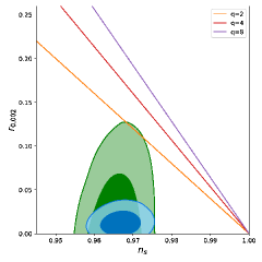
Figure 4: Comparison of observational constraints with $x_{*}\simeq 1$ models. The contours are the same as in figure 1.

So far we have considered models for which cosmological scales exit the horizon either when $x_{*}\ll 1$ or $x_{*}\gg 1$. In this section we look for observationally acceptable models with $x_{*}\simeq 1$. To that aim, let us define

$$\delta \equiv 1-x^{2}\,,$$ (167)

where $\left|\delta\right|\ll 1$.

Before doing the analysis note that in this setup the constraints on $p$ in eq. (138) do not apply. Indeed, close to $x\simeq 1$ the gravitational force is always directed towards the minimum of the potential, as can be confirmed by writing

$$U_{,x} = 2U\left[-\frac{q-\left(q-p\right)\delta}{\left(1-\frac{1}{2}\delta\right)\delta}\right]\,.$$ (168)

For $x\lesssim 1$ $\delta$ is positive, which makes $U_{,x}$ negative and vice versa.

Taking the first two terms in the expansion of $\epsilon_{U}$ in terms of $\delta^{-1}$ we can write

$$\epsilon_{U} \simeq \frac{4p^{2}\xi^{2/p}}{2+3p^{2}\xi^{2/p}}\left(\frac{q}{p}\right)^{2}\frac{1}{\delta^{2}}\,.$$ (169)

It follows that slow-roll inflation, with $\epsilon_{U}\ll 1$, can be realised only for

$$p^{2}\xi^{2/p} \ll 1\,,$$ (170)

that is $F_{,\phi}^{2}\ll F$. Using this fact the above equation for $\epsilon_{U}$ can be simplified:

$$\epsilon_{U} \simeq \frac{2q^{2}\xi^{2/p}}{\delta^{2}}\,.$$ (171)

Applying the same approximations to the expression of $\eta_{FV}$ in eq. (111) we get

$$\eta_{FV} \simeq \frac{4q\xi^{2/p}}{\delta^{2}}\,.$$ (172)

Plugging in the last two results into eqs. (114) and (115) one finally arrives at

$$n_{\mathrm{s}}-1 \simeq -\frac{q+2}{8q}r\,.$$ (173)

The smallest $r$ value for a given $n_{\mathrm{s}}$ is achieved with $q=2$. However, as can be seen in fig. 4, even for these values the predictions lie outside the $2\sigma$ contour of the BICEP/Keck results.

Our results of section V are summarised in table 1.

		$F_{,\phi*}^{2}\ll F_{*}$	$F_{,\phi*}^{2}\gg F_{*}$
Hilltop ($x_{*}\ll 1$)		eq. (145): $n_{\mathrm{s}}-1\simeq\frac{2-3p}{16p}r$	no slow-roll
Chaotic ($x_{*}\gg 1$)	$q>p$	eq. (153): $n_{\mathrm{s}}-1\simeq\frac{3\left(p-2\right)-2\left(q-2\right)}{16\left(q-p\right)}r$	no slow-roll
	$q=p=6$	eq. (157): $n_{\mathrm{s}}-1\simeq-\frac{r}{6}$	eq. (161): $n_{\mathrm{s}}-1\simeq-\frac{2}{p}\sqrt{\frac{r}{3}}-\left(\frac{4}{p}+1\right)\frac{r}{8}$
	$q=p\neq 6$	eq. (158): $n_{\mathrm{s}}-1\simeq\frac{p-6}{p}x_{*}^{2}\epsilon_{U}$
$x_{*}\simeq 1$		eq. (173): $n_{\mathrm{s}}-1\simeq-\frac{q+2}{8q}r$	no slow-roll

Table 1: The summary of observational predictions of the generalised induced gravity inflation models in different regimes. In this table “no slow-roll” signifies the absence of $\epsilon_{U}\ll 1$ region. The only models that are compatible with observations are chaotic type models with $p=q\leq 6$ in the regime $F_{,\phi*}^{2}\gg F_{*}$ (see fig. 2b).

VI Summary and Conclusions

In this work we consider inflation models within the framework of scalar-tensor theories of gravity. The most straightforward way to analyse such models and confront them with observations is to transform the action into the Einstein frame. But this is not always desirable. For example, after the transformation the matter sector directly couples to the scalar field, even if no such coupling is introduced in the Jordan frame. For certain applications this might actually complicate the analysis. In those cases, it would be convenient to have a formalism where inflation observables can be calculated only relying on Jordan frame quantities. In this work we derive the requirements that Jordan frame quantities must satisfy to provide slow-roll inflation. We also derive Jordan frame flow and slow-roll parameters which must be small, and write inflation observables in terms of those parameters.

The central idea of our method is to utilise the fact that conformal transformation corresponds to the change of units of measure [45]. We assume to slice the spacetime into spacelike hypersurfaces and keep that slicing fixed. It allows us to map the relations defined in the Einstein frame to the Jordan frame on the same slice by changing the units of measure (performing the conformal transformation). In particular, we take the conditions required for inflation and more stringent conditions for slow-roll inflation, which are most clearly defined in the Einstein frame, and map them to the Jordan frame.

We also make use of another convenient fact that the scalar and tensor metric perturbation spectra in single field slow-roll inflation models can be conveniently written in terms of homogeneous quantities only. Hence, only the homogeneous relations need to be mapped from the Einstein to the Jordan frame in order to derive observable model predictions.

Using this method we first derive the conditions for inflation. It has been noted in various places in the literature (see e.g. [10]) that those conditions in the Jordan frame might look somewhat counterintuitive from the Einstein frame perspective. For example, the Jordan frame scale factor does not have to be accelerating, as was demonstrated in eq. (73). Or the Hubble flow parameter $\epsilon_{1}$ does not have to be smaller than 1 (see eq. (71)). This has to be kept in mind when doing computations that are related to the end of inflation.

However, once we impose a much stronger requirement, that the Einstein frame Hubble-flow parameter $\hat{\epsilon}_{1}\ll 1$ (see eq. (6) for the definition), the conditions become more stringent. In that case some of the familiar expressions in the Einstein frame can be carried over to the Jordan one. In particular eqs. (78) and (86), which for convenience we rewrite here, are

$$\frac{1}{2}\dot{\phi}^{2} \ll V\,,$$

$$\frac{\dot{V}}{HV} \ll 1\,.$$

In the Jordan frame we have an additional function $F$. Which enlarges the number of conditions. To find a compact parametrisation for them we introduced a number of “flow parameters”, in analogy to the “Hubble-flow parameters”. These are $\epsilon_{i}$, $\theta_{i}$ and $\gamma^{2}$ defined in eqs. (65) - (67). We demonstrated in this work that the requirement $\hat{\epsilon}_{i}\ll 1$ translates into the Jordan frame as

$$\epsilon_{1},\>\gamma^{2},\>\left|\gamma_{2}\right|,\>\left|\theta_{1}\right|,\>\left|\theta_{1}\theta_{2}\right|\ll 1\,.$$

The above realtions are derived in eqs. (89), (92), (88), (82) and (95) respectively.

Only two of the three sets of parameters $\epsilon_{i}$, $\theta_{i}$ and $\gamma_{i}$ are needed to describe the system. And we found that using $\theta_{i}$ and $\gamma_{i}$ results in the most compact equations. However, when computing inflation observables we provide two combinations. In eqs. (96)-(98) the scalar spectral index, scalar spectral tilt and tensor-to-scalar ratio, $A_{\mathrm{s}}$, $n_{\mathrm{s}}$ and $r$ respectively, are written as functions of $\gamma_{i}$ and $\theta_{i}$

$$A_{\mathrm{s}} \simeq\frac{V}{24\pi^{2}F^{2}\gamma^{2}}\,,$$

$$n_{\mathrm{s}}-1 \simeq-2\left(\gamma^{2}+\gamma_{2}-\theta_{1}\theta_{2}\right)\,,$$

$$r \simeq 16\gamma^{2}\,.$$

And in eqs. (100)-(102), they are written as functions of $\epsilon_{i}$ and $\theta_{i}$.

We also derive the slow-roll equations in the Jordan frame. As described above, we take the Einstein frame version of slow-roll conditions in eqs. (47) and (48) and after the conformal transformation they can be written as in eqs. (74) and (76). Taking into account all the smallness conditions discussed above we finally arrive at eqs. (83) and (85)

$$H^{2} \simeq\frac{V}{3F}\,,$$

$$3H\dot{\phi} \simeq\frac{2VF_{,\phi}-FV_{,\phi}}{F^{2}\mathcal{K}}\,,$$

which are the Jordan frame versions of the slow-roll Friedman equation and equation of motion. These approximate relations can be applied as long as slow-roll conditions $\epsilon_{U},\,\left|\eta_{FV}\right|\ll 1$ are satisfied, where the slow-roll parameters are defined in eqs. (109) and (111)

$$\epsilon_{U} =\frac{1}{2\mathcal{K}}\left(\frac{V_{,\phi}}{V}-2\frac{F_{,\phi}}{F}\right)^{2}\,,$$

$$\eta_{FV} =\frac{1}{\mathcal{K}}\left[2\frac{F_{,\phi\phi}}{F}-\frac{V_{,\phi\phi}}{V}-2\frac{F_{,\phi}^{2}}{F^{2}}+\frac{V_{,\phi}^{2}}{V^{2}}+\frac{\mathcal{K}_{,\phi}}{2\mathcal{K}}\left(\frac{V_{,\phi}}{V}-2\frac{F_{,\phi}}{F}\right)\right]\,,$$

where $\epsilon_{U}$ is the same slow-roll parameter as in the Einstein frame but expressed in terms of the Jordan frame quantities. The dependence of inflation observables on $\epsilon_{U}$ and $\eta_{FV}$ is given in eqs. (113)-(115)

$$A_{\mathrm{s}} \simeq \frac{V}{24\pi^{2}F^{2}\epsilon_{U}}\,,$$

$$n_{\mathrm{s}}-1 \simeq -2\left(\epsilon_{U}+\eta_{FV}\right)\,,$$

$$r \simeq 16\epsilon_{U}\,.$$

When computing numerical values of the above parameters, another aspect that has to be taken into account is the difference between the number of e-folds of inflation as defined with respect to $\hat{a}$ and $a$, i.e. the scale factors in the Einstein and Jordan frames respectively. This difference is proportional to the logarithm of $F$, as shown in eq. (105)

$$\hat{N}=N+\frac{1}{2}\ln\frac{F_{\mathrm{end}}}{F}\,.$$

Although the e-fold shift number $\ln\sqrt{F_{\mathrm{end}}/F}$ is logarithmic, it can be substantial and therefore generically cannot be neglected, as we demonstrate this in the case of induced gravity models of inflation. When comparing with observations, we used $\hat{N}$ from 50 to 60, which are the values used by the Planck team.

Finally, we should also mention another known fact, that in the Jordan frame the field does not necessarily roll down the potential $V\left(\phi\right)$ even in slow-roll. As the strength and the direction of the gravitational force depends on $F\left(\phi\right)$, the field $\phi$ can as well climb up that potential. This can be readily understood by looking at the gradient of the scalar field potential in the Einstein frame in eq. (64). The direction of the gravitational force is no longer determined solely by the gradient of $V\left(\phi\right)$, but in combination with the gradient of $F\left(\phi\right)$. This has to be taken into account when considering models of inflation, as we also demonstrate in our example model in section V.

In that section we consider a generalised induced gravity model. The main idea of induced gravity theories is to generate gravity by a spontaneous symmetry breaking [66, 67, 68, 69]. That is, General Relativity is recovered after the $\phi$ field settles at its VEV, which is determined by the potential $V\left(\phi\right)$. To make sure that the field slowly rolls towards the minimum of $V\left(\phi\right)$ one needs to constraint possible functional forms of $F\left(\phi\right)$.

The main goal of section V is to apply some of our results to a concrete model. Making use of Jordan frame quantities only we analyse the model specified in eqs. (131) and (132) and look for observationally acceptable parameter space. We found that, among the many regions where slow roll inflation could be realised, only the case with $p=q=2,\,4$ and $6$ in the “chaotic type” regime (where $\left|\phi_{*}\right|\gg\left|v\right|$) fall within $2\sigma$ region of the newest BICEP/Keck results [65] (see figure 2b).

Finally, to validate our method we performed numerical simulations in which we solved exact perturbation equations in the Einstein frame and compared them with our Jordan frame slow-roll approximations. As can be seen in the Appendix A and figure 2b the agreement is very good indeed.

In this work we neglected a possible contribution from matter fields to the dynamics of the system. We also analysed single field models only. These simplifications allowed a simple check of the above results by transforming the action into the Einstein frame and performing exact computations numerically. In the future we plan to extend our formalism by including those complications, such as matter fields and considering multi-field models, which will bring us closer to the real motivation of this work.

Appendix A Comparison of Flow Parameters with Numerical Simulations

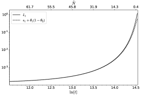
(a) Numerical check of eq. (107), where $\gamma$ is approximated by eq. (99).

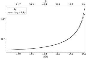
(b) Numerical check of eq. (94).

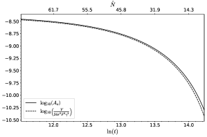
(c) Numerical check of eq. (96).

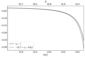
(d) Numerical check of eq. (97).

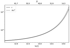
(e) Numerical check of eq. (98).

Figure 5: The comparison of exact, numerical Einstein frame results and approximate relations derived in this work. We used the model defined in eqs. (131) and (132) with $p=q=2$. These functions are plotted against the time $t$, which enumerates spatial slices and are shown on the lower horizontal axis. The upper horizontal axis shows the corresponding e-fold number $\hat{N}\left(t\right)$ in the Einstein frame for the reference.

To see how well our approximations perform we compared them with exact numerical solutions. To that purpose we used the induced gravity model in eqs. (131) and (132) with $p=q=2$ and $\phi_{*}/v\gg 1$. As shown in figure 2b this model conforms to observations very well.

The numerical simulations are performed in both frames. In the case of Einstein frame, we first transform the Jordan frame action in eq. (53) using the conformal transformation in eq. (16). This results in a scalar field with a non-canonical kinetic function as in eq. (25) and background equations (26), (30) and (31). Using eq. (51) they can be also expressed in terms of the number of e-folds $\hat{N}$

$$\frac{\mathrm{d}^{2}\phi}{\mathrm{d}\hat{N}^{2}}-\left(3-\frac{1}{\hat{H}}\frac{\mathrm{d}\hat{H}}{\mathrm{d}\hat{N}}\right)\frac{\mathrm{d}\phi}{\mathrm{d}\hat{N}}+\frac{1}{2}\frac{\mathcal{K}_{,\phi}}{\mathcal{K}}\left(\frac{\mathrm{d}\phi}{\mathrm{d}\hat{N}}\right)^{2}+\frac{U_{,\phi}}{\mathcal{K}\hat{H}^{2}}=0\,,$$ (174)

$$\hat{H}^{2}=\frac{U\left(\phi\right)}{3-\frac{1}{2}\mathcal{K}\left(\frac{\mathrm{d}\phi}{\mathrm{d}\hat{N}}\right)^{2}}\,,$$ (175)

$$\frac{\mathrm{d}\hat{H}}{\mathrm{d}\hat{N}}=\frac{1}{2}\mathcal{K}\hat{H}\left(\frac{\mathrm{d}\phi}{\mathrm{d}\hat{N}}\right)^{2}\,,$$ (176)

where the kinetic term is given by

$$\mathcal{K}=\left(\frac{1}{\xi}+6\right)\frac{1}{\phi^{2}}\,,$$ (177)

and the lapse function $\hat{\mathcal{N}}=\sqrt{F}=\sqrt{\xi}\phi$.

Alongside homogeneous equations we also integrate equations for perturbations. The curvature perturbation $\hat{\mathcal{R}}_{k}$ is related to the field perturbations $\delta\phi_{k}$ by [21]

$$\hat{\mathcal{R}}_{k}=-\frac{\hat{u}_{k}}{\hat{a}\frac{\textrm{d}\phi}{\textrm{d}\hat{N}}\sqrt{\mathcal{K}}}\,,$$ (178)

where $\hat{u}_{k}\equiv\hat{a}\sqrt{\mathcal{K}}\delta\phi_{k}$ is the Mukhanov-Sasaki variable. The evolution of $\hat{\mathcal{R}}_{k}$ is governed by the equation

$$\ddot{\hat{\mathcal{R}}}_{k}+\left[\left(3+\hat{\epsilon}_{2}\right)\sqrt{F}-\frac{1}{2}\frac{\dot{F}}{\hat{H}F}\right]\hat{H}\dot{\hat{\mathcal{R}}}_{k}+F\frac{k^{2}}{\hat{a}^{2}}\hat{\mathcal{R}}_{k}=0\,.$$ (179)

In terms of the number of e-folds it can be written as

$$\frac{\mathrm{d}^{2}\hat{\mathcal{R}}_{k}}{\mathrm{d}\hat{N}^{2}}-\left(3-\hat{\epsilon}_{1}+\hat{\epsilon}_{2}\right)\frac{\mathrm{d}\hat{\mathcal{R}}_{k}}{\mathrm{d}\hat{N}}+\frac{k^{2}}{\hat{a}^{2}\hat{H}^{2}}\hat{\mathcal{R}}_{k}=0\,,$$ (180)

where the Hubble flow parameters $\hat{\epsilon}_{i}$ are defined in eq. (6). The above equation is solved starting from Bunch-Davies vacuum initial conditions

$$\hat{u}_{k,\mathrm{vac}}=\frac{1}{\sqrt{2k}}e^{ik/(\hat{a}\hat{H})}\,,$$ (181)

$\hat{N}=5$ e-folds before the horizon exit, which is defined as $k=\hat{a}\hat{H}$, until $\hat{N}=5$ e-folds after the horizon exit. The latter $5$ e-folds are added in order to make it certain that the decaying mode is negligible and $\hat{\mathcal{R}}_{k}$ remains constant afterwards, whereas we start integrating $5$ e-folds before horizon-crossing time to ensure that $k/(\hat{a}\hat{H})\gg 1$ so eq. (181) is a good approximation for the field perturbations.

The power spectrum of $\hat{\mathcal{R}}$ and the spectral tilt are computed using

$$A_{\mathrm{s}} = \frac{k^{3}}{2\pi^{2}}\left|\hat{\mathcal{R}}_{k}\right|^{2}\,,$$ (182)

and

$$n_{\mathrm{s}}-1 = \frac{\mathrm{d}\ln A_{\mathrm{s}}}{\mathrm{d}\ln k}\,.$$ (183)

Similarly we compute the amplitude of tensor perturbations. In terms of the number of $\hat{N}$ e-folds it is given by

$$\frac{\mathrm{d}^{2}\hat{h}_{k}}{\mathrm{d}\hat{N}^{2}}-\left(3-\hat{\epsilon}_{1}\right)\frac{\mathrm{d}\hat{h}_{k}}{\mathrm{d}\hat{N}}+\frac{k^{2}}{\hat{a}^{2}\hat{H}^{2}}\hat{h}_{k}=0\,,$$ (184)

with initial conditions

$$\hat{h}_{k,\mathrm{vac}}=2\frac{\hat{u}_{k,\mathrm{vac}}}{\hat{a}}.\$$ (185)

The tensor-to-scalar ratio is given by

$$r\equiv\frac{A_{\mathrm{t}}}{A_{\mathrm{s}}}\,,$$ (186)

where the tensor amplitude is defined by

$$A_{\mathrm{t}} = \frac{k^{3}}{2\pi^{2}}\left|\hat{h}_{k}\right|^{2}\,.$$ (187)

As we integrate eqs. (174)-(176) and (180), (184) we also compute the coordinate time, using eq. (51)

$$t_{\textrm{end}}-t=\intop_{0}^{\hat{N}}\frac{\mathrm{d}\hat{N}}{\sqrt{F}\hat{H}}\,,$$ (188)

where $t_{\textrm{end}}>t$ and $t_{\mathrm{end}}$ is an arbitrary value at the end of inflation.

In the Jordan frame we only need to integrate homogeneous equations. To make sure we start from the same spatial slice, the initial values of $\phi$ and $\dot{\phi}$ are taken exactly the same as in the simulations above. Then, using definitions of $\hat{N}$ and $N$ in eqs. (51) and (103) together with eqs. (59), (60) we can relate the derivatives in both frames by

$$\frac{\mathrm{d}\phi}{\mathrm{d}N}=\frac{1}{1+\frac{F_{,\phi}}{2F}\frac{\mathrm{d}\phi}{\mathrm{d}\hat{N}}}\frac{\mathrm{d}\phi}{\mathrm{d}\hat{N}}\,.$$ (189)

The homogeneous system of Jordan frame equations that we are solving are given in eqs. (61)-(63). In terms of e-fold numbers $N$ they can be written as

$$\frac{\textrm{d}^{2}\phi}{\textrm{d}N^{2}}-\left(3-\epsilon_{1}\right)\frac{\textrm{d}\phi}{\textrm{d}N}+\frac{V_{,\phi}}{H^{2}}=3F_{,\phi}\left(2-\epsilon_{1}\right),$$ (190)

$$H^{2}=\frac{V}{3F}\frac{1}{1-\frac{1}{6F}\left(\frac{\textrm{d}\phi}{\textrm{d}N}\right)^{2}+2\theta_{1}},$$ (191)

$$\epsilon_{1}=-\frac{\left(\frac{\textrm{d}\phi}{\textrm{d}N}\right)^{2}+\frac{\textrm{d}F}{\textrm{d}N}+\frac{\textrm{d}^{2}F}{\textrm{d}N^{2}}}{2F\left(1+\theta_{1}\right)},$$ (192)

where $\theta_{1}$ is defined in eq. (66). The coordinate time is calculated by integrating (c.f. eq. (103))

$$t_{\textrm{end}}-t=\intop_{0}^{N}\frac{\mathrm{d}N}{H}\,.$$ (193)

Having computed the time variable $t$ in both frames, we can compare the results from the Jordan and Einstein frames on the same time slice. The results are shown in figure 5. In that figure we compare the exact Einstein frame calculations with the corresponding Jordan frame slow-roll approximations. In particular, in figures 5a and 5b we see that the agreement between the first two Einstein frame Hubble flow parameters and their expressions in terms of Jordan frame flow parameters agree very well. While looking at figures 5c, 5d and 5e we can conclude the same about the exact simulations of inflation observables and their approximate expressions in terms of Jordan frame flow parameters.

We can also check numerically the exact relation between $\hat{N}$ and $N$ in eq. (105). We plot their values on the same spatial slice in figure 6. As one can see, adding the e-fold shift number makes both curves, $\hat{N}\left(t\right)$ and $N\left(t\right)$, overlap exactly.

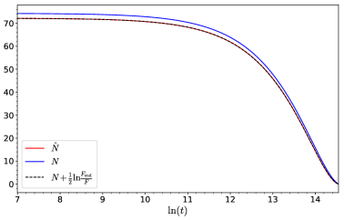
Figure 6: The e-fold number in each frame after solving numerically the exact field equations. We show the effect of the e-fold shift number as in eq. (105).

- [1] A.A. Starobinsky, A new type of isotropic cosmological models without singularity, Phys. Lett. B91 (1980) 99.
- [2] D. La and P.J. Steinhardt, Extended Inflationary Cosmology, Phys. Rev. Lett. 62 (1989) 376.
- [3] J. McDonald, Chaotic inflation in Brans-Dicke models, Phys. Rev. D 44 (1991) 2314.
- [4] P.J. Steinhardt and F.S. Accetta, Hyperextended inflation, Phys. Rev. Lett. 64 (1990) 2740.
- [5] B. Spokoiny, Inflation and generation of perturbations in broken-symmetric theory of gravity, Phys.Lett. B147 (1984) 39.
- [6] F.S. Accetta, D.J. Zoller and M.S. Turner, Induced Gravity Inflation, Phys. Rev. D 31 (1985) 3046.
- [7] F. Lucchin, S. Matarrese and M.D. Pollock, Inflation With a Nonminimally Coupled Scalar Field, Phys. Lett. B 167 (1986) 163.
- [8] F.L. Bezrukov and M. Shaposhnikov, The standard model higgs boson as the inflaton, Phys. Lett. B659 (2008) 703 [0710.3755].
- [9] D.H. Coule, Pre-big bang model has Planck problem, Class. Quant. Grav. 15 (1998) 2803 [gr-qc/9712062].
- [10] V. Faraoni, Cosmology in scalar tensor gravity, Springer Dordrecht, 1 ed. (2004), 10.1007/978-1-4020-1989-0.
- [11] D. Lyth and A. Liddle, The Primordial Density Perturbation: Cosmology, Inflation and the Origin of Structure, Cambridge University Press (2009).
- [12] E.D. Stewart and D.H. Lyth, A more accurate analytic calculation of the spectrum of cosmological perturbations produced during inflation, Phys.Lett. B302 (1993) 171 [gr-qc/9302019].
- [13] J.-O. Gong and E.D. Stewart, The Density perturbation power spectrum to second order corrections in the slow roll expansion, Phys. Lett. B 510 (2001) 1 [astro-ph/0101225].
- [14] S.M. Leach, A.R. Liddle, J. Martin and D.J. Schwarz, Cosmological parameter estimation and the inflationary cosmology, Phys. Rev. D 66 (2002) 023515 [astro-ph/0202094].
- [15] Planck collaboration, Planck 2018 results. X. constraints on inflation, Astron. Astrophys. 641 (2020) A10 [1807.06211].
- [16] Planck collaboration, Planck 2013 results. XXII. Constraints on inflation, Astron. Astrophys. 571 (2014) A22 [1303.5082].
- [17] V. Domcke and K. Schmitz, Inflation from High-Scale Supersymmetry Breaking, Phys. Rev. D 97 (2018) 115025 [1712.08121].
- [18] P. Kuusk, M. Rünkla, M. Saal and O. Vilson, Invariant slow-roll parameters in scalar-tensor theories, Class. Quant. Grav. 33 (2016) 195008 [1605.07033].
- [19] J.C. Hwang, Cosmological perturbations in generalized gravity theories: Formulation, Class. Quant. Grav. 7 (1990) 1613.
- [20] J.C. Hwang, Cosmological perturbations in generalized gravity theories: Solutions, Phys. Rev. D 42 (1990) 2601.
- [21] J.-c. Hwang and H. Noh, Cosmological perturbations in generalized gravity theories, Phys.Rev. D54 (1996) 1460.
- [22] R. Myrzakulov, L. Sebastiani and S. Vagnozzi, Inflation in -theories and mimetic gravity scenario, Eur. Phys. J. C 75 (2015) 444 [1504.07984].
- [23] E. Elizalde, S.D. Odintsov, V.K. Oikonomou and T. Paul, Logarithmic-corrected Gravity Inflation in the Presence of Kalb-Ramond Fields, JCAP 02 (2019) 017 [1810.07711].
- [24] R. Fakir, Quantum creation of universes with nonminimal coupling, Phys. Rev. D 41 (1990) 3012.
- [25] N. Makino and M. Sasaki, The Density perturbation in the chaotic inflation with nonminimal coupling, Prog. Theor. Phys. 86 (1991) 103.
- [26] J.-O. Gong, J.-c. Hwang, W.-I. Park, M. Sasaki and Y.-S. Song, Conformal invariance of curvature perturbation, JCAP 1109 (2011) 023 [1107.1840].
- [27] J. White, M. Minamitsuji and M. Sasaki, Curvature perturbation in multi-field inflation with non-minimal coupling, JCAP 1207 (2012) 039 [1205.0656].
- [28] T. Kubota, N. Misumi, W. Naylor and N. Okuda, The Conformal Transformation in General Single Field Inflation with Non-Minimal Coupling, JCAP 02 (2012) 034 [1112.5233].
- [29] R. Catena, M. Pietroni and L. Scarabello, Einstein and Jordan reconciled: a frame-invariant approach to scalar-tensor cosmology, Phys. Rev. D 76 (2007) 084039 [astro-ph/0604492].
- [30] R. Catena, M. Pietroni and L. Scarabello, Local transformations of units in scalar-tensor cosmology, J. Phys. A 40 (2007) 6883 [hep-th/0610292].
- [31] A. Racioppi and M. Vasar, On the number of e-folds in the Jordan and Einstein frames, Eur. Phys. J. Plus 137 (2022) 637 [2111.09677].
- [32] D.I. Kaiser, Frame independent calculation of spectral indices from inflation, Submitted to: Phys. Lett. B (1995) [astro-ph/9507048].
- [33] T. Prokopec and J. Weenink, Frame independent cosmological perturbations, JCAP 09 (2013) 027 [1304.6737].
- [34] L. Järv, K. Kannike, L. Marzola, A. Racioppi, M. Raidal, M. Rünkla et al., Frame-Independent Classification of Single-Field Inflationary Models, Phys. Rev. Lett. 118 (2017) 151302 [1612.06863].
- [35] J. Garcia-Bellido, A.D. Linde and D.A. Linde, Fluctuations of the gravitational constant in the inflationary Brans-Dicke cosmology, Phys. Rev. D 50 (1994) 730 [astro-ph/9312039].
- [36] D.F. Torres, Slow roll inflation in nonminimally coupled theories: Hyperextended gravity approach, Phys. Lett. A 225 (1997) 13 [gr-qc/9610021].
- [37] J.R. Morris, Generalized slow roll conditions and the possibility of intermediate scale inflation in scalar tensor theory, Class. Quant. Grav. 18 (2001) 2977 [gr-qc/0106022].
- [38] T. Chiba and M. Yamaguchi, Extended slow-roll conditions and rapid-roll conditions, JCAP 0810 (2008) 021 [0807.4965].
- [39] K. Akın, A. Savaş Arapoglu and A. Emrah Yükselci, Formalizing slow-roll inflation in scalar-tensor theories of gravitation, Phys. Dark Univ. 30 (2020) 100691 [2007.10850].
- [40] L. Järv and A. Toporensky, Global portraits of nonminimal inflation, Eur. Phys. J. C 82 (2022) 179 [2104.10183].
- [41] E.E. Flanagan, The Conformal frame freedom in theories of gravitation, Class. Quant. Grav. 21 (2004) 3817 [gr-qc/0403063].
- [42] V. Faraoni and S. Nadeau, The (pseudo)issue of the conformal frame revisited, Phys.Rev. D75 (2007) 023501 [gr-qc/0612075].
- [43] H. Azri, Are there really conformal frames? Uniqueness of affine inflation, Int. J. Mod. Phys. D 27 (2018) 1830006 [1802.01247].
- [44] E. Gourgoulhon, 3+1 formalism and bases of numerical relativity, gr-qc/0703035.
- [45] R. Dicke, Mach’s principle and invariance under transformation of units, Phys. Rev. 125 (1962) 2163.
- [46] N.D. Birrell and P.C.W. Davies, Quantum Fields in Curved Space, Cambridge Monographs on Mathematical Physics, Cambridge University Press, Cambridge, UK (2, 1984), 10.1017/CBO9780511622632.
- [47] N. Deruelle and M. Sasaki, Conformal equivalence in classical gravity: the example of ’Veiled’ General Relativity, Springer Proc. Phys. 137 (2011) 247 [1007.3563].
- [48] G. Domènech and M. Sasaki, Conformal frames in cosmology, in 2nd LeCosPA Symposium: Everything about Gravity, Celebrating the Centenary of Einstein’s General Relativity (LeCosPA2015) Taipei, Taiwan, December 14-18, 2015, 2016, http://inspirehep.net/record/1422742 [1602.06332].
- [49] E. Poisson, A Relativist’s Toolkit: The Mathematics of Black-Hole Mechanics, Cambridge University Press (12, 2009), 10.1017/CBO9780511606601.
- [50] M. Fierz, On the physical interpretation of P.Jordan’s extended theory of gravitation, Helv. Phys. Acta 29 (1956) 128.
- [51] C. Brans and R.H. Dicke, Mach’s principle and a relativistic theory of gravitation, Phys. Rev. 124 (1961) 925.
- [52] T. Kodama and T. Takahashi, Relaxing inflation models with nonminimal coupling: A general study, Phys. Rev. D 105 (2022) 063542 [2112.05283].
- [53] V. Faraoni, Generalized slow roll inflation, Phys. Lett. A 269 (2000) 209 [gr-qc/0004007].
- [54] A. Karam, T. Pappas and K. Tamvakis, Frame-dependence of higher-order inflationary observables in scalar-tensor theories, Phys. Rev. D 96 (2017) 064036 [1707.00984].
- [55] R.N. Lerner and J. McDonald, Higgs Inflation and Naturalness, JCAP 1004 (2010) 015 [0912.5463].
- [56] T. Futamase and K.-i. Maeda, Chaotic inflationary scenario in models having nonminimal coupling with curvature, Phys. Rev. D 39 (1989) 399.
- [57] S.C. Hyun, J. Kim, S.C. Park and T. Takahashi, Non-minimally assisted chaotic inflation, JCAP 05 (2022) 045 [2203.09201].
- [58] M.D. Pollock and D. Sahdev, Pole Law Inflation in a Theory of Induced Gravity, Phys. Lett. B 222 (1989) 12.
- [59] D.I. Kaiser, Constraints in the context of induced gravity inflation, Phys. Rev. D 49 (1994) 6347 [astro-ph/9308043].
- [60] J.L. Cervantes-Cota and H. Dehnen, Induced gravity inflation in the SU(5) GUT, Phys. Rev. D 51 (1995) 395 [astro-ph/9412032].
- [61] R. Fakir and W.G. Unruh, Induced gravity inflation, Phys. Rev. D 41 (1990) 1792.
- [62] D.S. Salopek, J.R. Bond and J.M. Bardeen, Designing Density Fluctuation Spectra in Inflation, Phys. Rev. D40 (1989) 1753.
- [63] D.I. Kaiser, Induced gravity inflation and the density perturbation spectrum, Phys. Lett. B 340 (1994) 23 [astro-ph/9405029].
- [64] D.I. Kaiser, Primordial spectral indices from generalized Einstein theories, Phys. Rev. D52 (1995) 4295 [astro-ph/9408044].
- [65] BICEP, Keck collaboration, Improved Constraints on Primordial Gravitational Waves using Planck, WMAP, and BICEP/Keck Observations through the 2018 Observing Season, Phys. Rev. Lett. 127 (2021) 151301 [2110.00483].
- [66] A.D. Sakharov, Vacuum quantum fluctuations in curved space and the theory of gravitation, Dokl. Akad. Nauk Ser. Fiz. 177 (1967) 70.
- [67] J. O’Hanlon, Intermediate-range gravity: a generally covariant model, Phys. Rev. Lett. 29 (1972) 137.
- [68] A. Zee, A Broken Symmetric Theory of Gravity, Phys. Rev. Lett. 42 (1979) 417.
- [69] L. Smolin, Towards a Theory of Space-Time Structure at Very Short Distances, Nucl. Phys. B 160 (1979) 253.