Clustering of emission line galaxies with IllustrisTNG I.: fundamental properties and halo occupation distribution

Abstract

Upcoming spectroscopic redshift surveys use emission line galaxies (ELGs) to trace the three-dimensional matter distributions with wider area coverage in the deeper Universe. Since the halos hosting ELGs are young and undergo infall towards more massive halos along filamentary structures, contrary to a widely employed luminous red galaxy sample, the dynamics specific to ELGs should be taken into account to refine the theoretical modelling at non-linear scales. In this paper, we scrutinise the halo occupation distribution (HOD) and clustering properties of ELGs by utilising IllustrisTNG galaxy formation hydrodynamical simulations. Leveraging stellar population synthesis technique coupled with the photo-ionization model, we compute line intensities of simulated galaxies and construct mock H$\alpha$ and [O ii] ELG catalogues. The line luminosity functions and the relation between the star formation rate and line intensity are well consistent with observational estimates. Next, we measure the HOD and demonstrate that there is a distinct population for the central HOD, which corresponds to low-mass infalling halos. We then perform the statistical inference of HOD parameters from the projected correlation function. Our analysis indicates that the inferred HODs significantly deviate from the HOD measured directly from simulations although the best-fit model yields a good fit to the projected correlation function. It implies that the information content of the projected correlation function is not adequate to constrain HOD models correctly and thus, it is important to employ mock ELG catalogues to calibrate the functional form of HOD models and add prior information on HOD parameters to robustly determine the HOD.

1 Introduction

Matter fluctuations generated during the inflationary era are amplified through gravitational instability driven primarily by dark matter, resulting in hierarchical structures which range from stars to galaxy clusters (White & Frenk, 1991). Thus, the nature of dark matter and gravitational physics is imprinted onto the formation and evolution of the large-scale structures (LSS) of the Universe (for a review, see Weinberg et al., 2013). In addition, dark energy induces accelerated expansion of the Universe and has considerable impacts on the geometry of the Universe. The geometry of the Universe is robustly measured from the acoustic scale of sound waves in the cosmic baryon-photon fluid, referred to as baryon acoustic oscillation (BAO). The BAO scale serves as the standard ruler of the Universe, and the measurement of the scale can tightly constrain cosmological parameters (Eisenstein et al., 2005; Aubourg et al., 2015). Though the fundamental information of the Universe is embedded into the matter distribution, it is dominated by dark matter invisible to optical telescopes. Instead, one can use galaxies as surrogates for the matter distribution because they generally form in dense regions and thus are expected to trace the matter distribution. To do this, galaxy clustering analysis, which has been playing a central role in observational cosmology, is commonly exploited. However, since galaxy formation processes are governed by complex nonlinear astrophysics, the relation between galaxy and matter distributions becomes nonlinear, which makes it challenging to study it from the first principle. This galaxy bias (for a review, see Desjacques et al., 2018) is considered as a critical obstacle for galaxy clustering analysis to date.

In the last decade, various observational programmes, which aim to measure galaxy clustering and constrain cosmological models from it, have been conducted: extended Baryon Oscillation Spectroscopic Survey (eBOSS; Alam et al., 2021), 6dF Galaxy Survey (Beutler et al., 2011), WiggleZ (Blake et al., 2011), and VIPERS (de la Torre et al., 2017). Recently, wider and deeper spectroscopic surveys are being proposed to improve the accuracy: Subaru Prime Focus Spectrograph (PFS; Takada et al., 2014), Dark Energy Spectrograph Instrument (DESI; DESI Collaboration et al., 2016a, b), Euclid (Laureijs et al., 2011; Amendola et al., 2013), and Roman Space Telescope. These upcoming spectroscopic surveys will target a specific population of galaxies: emission line galaxies (ELGs). ELGs are characterized by the bright line emissions, e.g., H$\alpha$ ($\lambda\,6564.62\,\mathrm{\mathring{A}}$) or [O ii] ($\lambda\lambda\,3727.09\,\mathrm{\mathring{A}},3729.88\,\mathrm{\mathring{A}}$), which are sourced from circumstellar gas irradiated by massive OB-type stars. The lifetime of such massive stars is short and the nebular emission lasts only for $\simeq 10\,\mathrm{Myr}$ (Byler et al., 2017). In summary, the emission lines are an indicator of star-formation activity (Charlot & Longhetti, 2001; Kewley et al., 2019). The epoch at the redshift $z=1\text{--}2$ is called cosmic noon, where star formation is the most active over the cosmic history, and at this epoch, a large number of ELGs are expected to be detected. Several pilot surveys have measured ELG clustering around cosmic noon, e.g., HiZELS (Geach et al., 2008; Sobral et al., 2010) and FastSound (Tonegawa et al., 2015; Okada et al., 2016; Okumura et al., 2016). In the near future, large survey programmes will improve the number of detected ELGs and survey areas, and thus, the widest galaxy clustering analysis at the deepest Universe will be accessible.

To extract maximal information from the observed galaxy distribution, it is critical to develop accurate and precise theoretical models to predict statistics of galaxy clustering down to small (non-linear) scales. Spectroscopic redshift surveys used to target mainly stellar-mass limited samples, which are widely referred to as luminous red galaxies (LRGs; Eisenstein et al., 2001). In general, LRGs are red and quenched galaxies and thus are likely to be hosted by old and massive halos. So far, various theoretical models have been developed to predict LRG clustering. For example, the abundance matching technique (Vale & Ostriker, 2004; Conroy et al., 2006), which connects the luminosity of LRGs to halo properties, e.g., halo mass or circular velocity, can reproduce the observed correlation functions quite well. However, it is not trivial whether the same theoretical frameworks can be applicable to ELG clustering. In fact, previous works (Orsi & Angulo, 2018; Gonzalez-Perez et al., 2018, 2020) used semi-analytic simulations, which populate galaxies onto dark-matter-only $N$-body simulations based on the merger history of dark halos (Springel et al., 2005; Croton et al., 2016), highlighted the difference of LRG and ELG clustering; LRGs are well virialized in halos and located close to the halo centres but a majority of halos hosting ELGs is undergoing infall towards massive halos along filamentary structures. The nebular emission of ELGs lasts only for $10\,\mathrm{Myr}$, which corresponds to the lifetime of the central star, but the dynamical time scale of the hosting halo is $\gtrsim 100\,\mathrm{Myr}$. Therefore, it is expeted that a large fraction of the nebular emission is extinguished during the first passage to the pericentre. Furthermore, it is shown that the velocity distribution of ELGs within a host halo significantly deviates from Gaussian distribution due to the infall motion (Orsi & Angulo, 2018). This coherent dynamics specific to ELGs has appreciable impacts on theoretical modelling of the velocity field, i.e., ELG clustering in redshift space.

In order to shed light on the ELG clustering, galaxy formation hydrodynamical simulations are one of the most promising and powerful methods because the simulations can trace the evolution of LSS and the formation of ELGs simultaneously. The galaxy formation physics involves formation and evolution of various astronomical objects with the wide dynamic range; from $\mathrm{AU}$ scale for black holes to $\mathrm{Mpc}$ scale for galaxy clusters. Such multi-scale physics can be approximated as subgrid physics, which implements galaxy formation physics by coarse-graining in an ad-hoc manner (for a review, see Somerville & Davé, 2015). The subgrid hydrodynamical simulations can better reproduce observed quantities, such as stellar mass functions and black hole co-evolution, once free parameters are properly calibrated. In this paper, we exploit the hydrodynamical simulations to generate high-fidelity mock ELG catalogues and address clustering of the simulated ELGs for better understanding of clustering nature of ELGs. Compared to the semi-analytical approach, the key advantage of hydrodynamical simulations is that a wide variety of information, e.g., formation age, environments, and dynamics, are readily available and enable us to create more realistic ELG catalogues (Park et al., 2015; Shimizu et al., 2016; Favole et al., 2020; Hadzhiyska et al., 2021; Favole et al., 2022; Yuan et al., 2022). Therefore, it is possible to scrutinise the relation between the observed properties of ELGs and large-scale clustering, which reflects the physics of dark matter and dark energy. We construct mock catalogues of H$\alpha$ and [O ii] ELGs, which are targets of Euclid and PFS surveys, respectively, by leveraging the state-of-the-art hydrodynamical simulations, IllustrisTNG, coupled with the stellar population synthesis model. Then, we measure halo occupation distribution (HOD), i.e., the mean number of galaxies as the function of host halo mass, which is the straightforward way to relate ELGs to host halos. Finally, we measure the projected correlation function, which is one of major statistics used in actual observations, and carry out an HOD challenge, where we investigate how one can reproduce the underlying HOD from statistical analysis of the measured projected correlation function. In subsequent series of papers, we will present a cosmological parameter challenge analysis with correlation functions in redshift space and detailed analysis on ELG-halo connection, in particular assembly bias and velocity bias.

This paper is organized as follows. In Section 2, we present numerical methods to generate mock ELG catalogues used in this work: IllustrisTNG hydrodynamical simulations and post-processing with stellar population synthesis code PÉGASE-3. In Section 3, we overview HOD and theoretical modelling of projected correlation functions. In Section 4, we discuss the properties of mock ELGs and present the measurement of HODs of mock ELGs. In Section 5, we constrain HOD model parameters from the direct measurement of the HOD and the projected correlation function. We make a concluding remark in Section 6.

2 Numerical Simulations

In this section, we overview our numerical methods to produce the mock catalogues of H$\alpha$ and [O ii] ELGs.

2.1 Hydrodynamical simulations

As the backbone of our mock simulation suite, we utilise IllustrisTNG simulations (Nelson et al., 2018; Pillepich et al., 2018b; Springel et al., 2018; Naiman et al., 2018; Marinacci et al., 2018; Nelson et al., 2019). The simulations are run by the moving mesh code AREPO (Springel, 2010) and various baryonic processes are implemented as subgrid physics (Weinberger et al., 2017; Pillepich et al., 2018a). Among the realisations of the simulation suite, we use the run with the largest box, TNG300-1 (hereafter TNG300), where the length on a side is $205\,h^{-1}\,\mathrm{Mpc}$ in comoving coordinates, the number of dark matter particles and gas cells is $2500^{3}$ for each, and the corresponding mass resolution for dark matter and gas is $m_{\mathrm{DM}}=5.9\times 10^{7}\,h^{-1}\,M_{\sun}$ and $m_{\mathrm{gas}}=1.4\times 10^{6}\,h^{-1}\,M_{\sun}$, respectively. The simulation snapshots are densely sampled in the wide range of redshifts $z=0\text{--}20$. Unless stated, we use the snapshot at the redshift $z=1.5$, which is the typical redshift for future spectroscopic surveys.

Throughout this paper, a flat $\Lambda$-cold dark matter Universe is assumed and cosmological parameters are best-fit parameters of the Planck 2015 results (Planck Collaboration et al., 2016), as used in the IllustrisTNG simulations; Hubble constant $H_{0}=67.74\,\mathrm{km}\,\mathrm{s}^{-1}\,\mathrm{Mpc}^{-1}$, the baryon density $\Omega_{\mathrm{b}}=0.0486$, the total matter density $\Omega_{\mathrm{m}}=0.3089$, the spectral index of scalar perturbations $n_{\mathrm{s}}=0.9667$, and the amplitude of matter fluctuations at $8\,h^{-1}\,\mathrm{Mpc}$ $\sigma_{8}=0.8159$. For neutrinos, we assume massless neutrinos with an effective number of neutrino species $N_{\mathrm{eff}}=3.046$.

2.2 Stellar population synthesis

Since the emission line intensities are not provided in the IllustrisTNG snapshots, we post-process the output to calculate spectral energy distributions (SEDs) of simulated galaxies based on stellar population synthesis (SPS). For this purpose, we employ the SPS code PÉGASE-3 (Fioc & Rocca-Volmerange, 2019), which calculates SEDs from far-IR to UV wavelengths and also computes the nebular emission intensities based on the photo-ionization code CLOUDY (Ferland et al., 2017). In PÉGASE-3, we adopt the initial mass function of Chabrier (2003), Padova stellar evolutionary tracks (Bressan et al., 1993; Fagotto et al., 1994a, b, c; Girardi et al., 1996), stellar yields for low mass stars of Marigo (2001) and high mass stars of Portinari et al. (1998), and stellar spectra libraries of BaSeL v3.1 (Westera et al., 2002).

First, we run PÉGASE-3 for eight initial metallicities, $Z_{\mathrm{ini}}=(0.0,0.0001,0.0004,0.004,0.008,0.02,0.05,0.1)$, where CLOUDY precomputed tables are available, and then SEDs and line intensities are output every $1\,\mathrm{Myr}$ in the range of $0\text{--}100\,\mathrm{Myr}$. Thus, we construct a precomputed table for line intensity with respect to metallicity and age. Next, we compute line luminosities for each galaxy found in TNG300. The subhalo catalogues provide the list of stellar particles which constitute a subhalo, and we regard a subhalo as a simulated galaxy. The contribution from a single stellar particle is calculated by bi-linear interpolation with the precomputed table with respect to the formation age and the metallicity, both of which are available in particle snapshots. In a sense, we regard a stellar particle as a tiny isolated galaxy. Since the line intensity of the precomputed table is normalized by the stellar mass, we sum up all the particle contributions by multiplying the initial stellar mass at the formation time and the resultant sum is the line luminosity of the galaxy.

Since the interested emission lines are subject to absorption due to dusts (for a review, see Salim & Narayanan, 2020), the dust attenuation should be taken into account for observed line luminosities. Nelson et al. (2018) addressed the dust attenuation from unresolved and resolved dusts and found that the impact of the resolved dust is relatively small compared with the unresolved one. Hence, we consider only unresolved dust contribution for simplicity. Instead of a power-law extinction model (Charlot & Fall, 2000) for unresolved dust contribution adopted in previous studies, in our modelling, the PÉGASE-3 code computes the dust evolution within a galaxy and incorporates dust extinction due to dust grains in star-forming clouds and diffuse inter-stellar medium (for details, see Section 6.1 of Fioc & Rocca-Volmerange, 2019). As discussed in Section 4.1, this prescription gives reasonable estimates of dust attenuation effects.

3 Theory

In this section, we review theoretical models used to analyse the clustering of ELGs in this paper. We present the halo model of the projected correlation function and its covariance matrix in Sections 3.1 and 3.2, respectively. We then introduce halo occupation models to relate the ELGs to their host halos in Section 3.3.

3.1 Projected correlation function

In order to compute the statistics of spatial clustering of ELGs, we begin with the galaxy power spectrum. We adopt a halo model, where all galaxies are assumed to form inside the host dark halos. There are two types of galaxies according to the internal locations within a halo: central and satellite galaxies. The central galaxies are located at the centre of the hosting dark halos and in general, the most massive galaxies in the halo. The satellite galaxies are distributed following the density profile of the halos and a halo can host multiple satellite galaxies. Under the halo model prescription, the galaxy power spectrum has two contributions; clustering in a single halo denoted as the one-halo term $P_{\mathrm{1h}}$ and clustering between two distinct halos denoted as the two-halo term $P_{\mathrm{2h}}$. The expression of the galaxy power spectrum $P_{\mathrm{gg}}$ is given as

$$P_{\mathrm{gg}}(k,z)= P_{\mathrm{1h}}(k,z)+P_{\mathrm{2h}}(k,z),$$ (1)

$$P_{\mathrm{1h}}(k,z)= \frac{1}{n_{\mathrm{g}}^{2}}\int\!\!\differential{M}\derivative{n_{\mathrm{h}}}{M}(M,z)[2\langle N_{\mathrm{cen}}N_{\mathrm{sat}}\rangle\tilde{u}_{\mathrm{h}}(k,M,z)$$

$$+\langle N_{\mathrm{sat}}(N_{\mathrm{sat}}-1)\rangle\tilde{u}_{\mathrm{h}}^{2}(k,M,z)],$$ (2)

$$P_{\mathrm{2h}}(k,z)= \frac{1}{n_{\mathrm{g}}^{2}}\int\!\!\differential{M_{1}}\derivative{n_{\mathrm{h}}}{M}(M_{1},z)[\langle N_{\mathrm{cen}}\rangle+\langle N_{\mathrm{sat}}\rangle\tilde{u}_{\mathrm{h}}(k,M_{1},z)]$$

$$\times\int\!\!\differential{M_{2}}\derivative{n_{\mathrm{h}}}{M}(M_{2},z)[\langle N_{\mathrm{cen}}\rangle+\langle N_{\mathrm{sat}}\rangle\tilde{u}_{\mathrm{h}}(k,M_{2},z)]$$

$$\times P_{\mathrm{hh}}(k,M_{1},M_{2},z),$$ (3)

where $\langle N_{\mathrm{cen}}\rangle$ and $\langle N_{\mathrm{cen}}\rangle$ are mean occupation numbers of central and satellite galaxies in a halo with mass $M$, respectively, and $n_{\mathrm{g}}$ is the galaxy number density. For the halo mass function, $\differential{n_{\mathrm{h}}}/\differential{M}$, we adopt the fitting formula of Tinker et al. (2008). There are several assumptions made to derive the expressions above. First, the radial distribution of satellite galaxies follow the density profile of halos, and we adopt Navarro–Frenk–White (NFW) profile (Navarro et al., 1996, 1997). In order to specify the NFW profile, $\rho_{\mathrm{NFW}}(r;M,z)$, the halo radius and the concentration parameter, which is defined as the ratio between halo radius and density scale radius, have to be determined. We adopt the virial radius as the halo radius (Bryan & Norman, 1998) and the concentration-mass relation of Klypin et al. (2016) calibrated with $N$-body simulations. The function $\tilde{u}_{\mathrm{h}}(k;M,z)$ is the Fourier transform of the scaled density profile, $\rho_{\mathrm{NFW}}(r;M,z)/M$, and we use the expression derived analytically by Scoccimarro et al. (2001). We assume that the central and satellite occupation numbers are independent, i.e., $\langle N_{\mathrm{cen}}N_{\mathrm{sat}}\rangle=\langle N_{\mathrm{cen}}\rangle\langle N_{\mathrm{sat}}\rangle$, and the satellite occupation follows the Poisson distribution $\langle N_{\mathrm{sat}}(N_{\mathrm{sat}}-1)\rangle=\langle N_{\mathrm{sat}}\rangle^{2}$. Regarding the cross-power spectrum of halos with masses $M_{1}$ and $M_{2}$, $P_{\mathrm{hh}}(k,M_{1},M_{2},z)$, higher-order bias contributions can be neglected at our interested scales and the non-linear effects can be incorporated by replacing the linear power spectrum with the non-linear one (van den Bosch et al., 2013). As a result, the cross-power spectrum is approximated as

$$P_{\mathrm{hh}}(k,M_{1},M_{2},z)=b_{\mathrm{h}}(M_{1},z)b_{\mathrm{h}}(M_{2},z)P_{\mathrm{NL}}(k,z),$$ (4)

where $b_{\mathrm{h}}(M,z)$ is the halo bias, for which we adopt the fitting formula calibrated with $N$-body simulations (Tinker et al., 2010). $P_{\mathrm{NL}}(k,z)$ is the non-linear matter power spectrum and we adopt the fitting formula based on the halofit prescription (Smith et al., 2003) with parameters calibrated in Takahashi et al. (2012).

Then, the galaxy three-dimensional correlation function $\xi_{\mathrm{gg}}$ is computed via a Hankel transform:

$$\xi_{\mathrm{gg}}(r,z)=\frac{1}{2\pi^{2}}\int k^{2}P_{\mathrm{gg}}(k,z)\frac{\sin(kr)}{kr}\differential{k},$$ (5)

where the FFTLog algorithm (Hamilton, 2000) is employed to compute the Hankel transform. Finally, the projected correlation function $w_{\mathrm{p}}(R,z)$ can be computed by projecting the three-dimensional correlation function along the line-of-sight direction:

$$w_{\mathrm{p}}(R,z)=2\int_{0}^{r_{\mathrm{max}}}\xi_{\mathrm{gg}}\left(r=\sqrt{R^{2}+r_{\pi}^{2}},z\right)\differential{r_{\pi}},$$ (6)

where $r_{\mathrm{max}}$ is the projection length and we fix $r_{\mathrm{max}}=50\,h^{-1}\,\mathrm{Mpc}$ throughout this paper.

3.2 Covariance matrix of the projected correlation function

In order to perform the statistical analysis with projected correlation functions, the statistical error estimation, i.e., covariance matrix, is an essential component. The most straightforward way to estimate the covariance matrix is to run many realisations of hydrodynamical simulations and compute the covariance among the realisations. However, this approach is not realistic due to the high computational costs of hydrodynamical simulations. There are several options to estimate the covariance matrix directly from the measurements such as the jackknife method. However, such methods are not able to estimate the covariance matrix at large scales. Therefore, we adopt the analytical method for covariance matrix calculations to exploit the measurements at all scales. To compute the covariance matrix of the projected correlation functions, we employ the Gaussian covariance matrix (Marian et al., 2015). The Gaussian covariance matrix is known to underestimate the covariance at small scales ($R\lesssim 5\,h^{-1}\,\mathrm{Mpc}$) due to the higher order contribution. However, such non-linearity can be partially incorporated by using non-linear galaxy power spectrum in Eq. (1). Thus, we employ the Gaussian covariance matrix for the statistical analysis.

The analytic expression of the Gaussian covariance matrix is given as

$$\mathrm{Cov}[w_{\mathrm{p}}](R_{i},R_{j})=\frac{2}{V_{\mathrm{s}}}\left\{2r_{\mathrm{max}}\int_{0}^{\infty}\frac{\differential{k_{\perp}}}{2\pi}k_{\perp}\bar{J}_{0}(k_{\perp}R_{i})\bar{J}_{0}(k_{\perp}R_{j})\right.$$

$$\left.\times P_{\mathrm{gg}}(k_{\perp})\left[P_{\mathrm{gg}}(k_{\perp})+\frac{2}{n_{\mathrm{g}}}\right]+\frac{\delta_{ij}^{\mathrm{K}}}{n_{\mathrm{g}}^{2}}\left[\bar{w}_{\mathrm{p}}(R_{i})+2r_{\mathrm{max}}\right]\right\},$$ (7)

where $\delta_{ij}^{\mathrm{K}}$ is the Kronecker delta, $V_{\mathrm{s}}$ is the survey volume, and $r_{\mathrm{max}}$ is the maximum projection length. In the above equation, we defined the bin-averaged Bessel function, $\bar{J}_{0}$, and projected correlation function, $\bar{w}_{\mathrm{p}}$, as

$$\bar{J}_{0}(k_{\perp}R_{i}) \equiv\frac{2\pi}{S_{R_{i}}}\int_{R_{i,\mathrm{min}}}^{R_{i,\mathrm{max}}}J_{0}(k_{\perp}R)R\differential{R},$$ (8)

$$\bar{w}_{\mathrm{p}}(R_{i}) \equiv\frac{2\pi}{S_{R_{i}}}\int_{R_{i,\mathrm{min}}}^{R_{i,\mathrm{max}}}w_{\mathrm{p}}(R)R\differential{R},$$ (9)

where the subscript $i$ denotes the transverse bin, $R_{i,\mathrm{min}}$ and $R_{i,\mathrm{max}}$ are lower and upper edges of the $i$-th radial bin, respectively, and $S_{R_{i}}=\pi\left(R_{i,\mathrm{max}}^{2}-R_{i,\mathrm{min}}^{2}\right)$.

3.3 Parametrisation of halo occupation distributions

One of the most fundamental quantities to characterize a dark halo is its mass, and thus, the occupation number of galaxies with respect to the halo mass, i.e., halo occupation distribution (HOD), is commonly used to relate the galaxies to their host halos (Jing et al., 1998; Peacock & Smith, 2000; Seljak, 2000; Ma & Fry, 2000; Scoccimarro et al., 2001; Cooray & Sheth, 2002; Berlind & Weinberg, 2002; Zheng et al., 2005; van den Bosch et al., 2013; Hikage et al., 2013; Okumura et al., 2015). In order to describe HOD of LRGs, Zheng et al. (2005) introduced the following functional form:

$$\langle N_{\mathrm{cen}}\rangle(M) =\frac{1}{2}\left[1+\mathrm{erf}\left(\frac{\log(M/M_{\mathrm{min}})}{\sigma_{\log M}}\right)\right],$$ (10)

$$\langle N_{\mathrm{sat}}\rangle(M) =\frac{1}{2}\left[1+\mathrm{erf}\left(\frac{\log(M/M_{\mathrm{min}})}{\sigma_{\log M}}\right)\right]\left(\frac{M-M_{0}}{M_{1}}\right)^{\alpha},$$ (11)

where $(M_{\mathrm{min}},\sigma_{\log M},M_{0},M_{1},\alpha)$ are free parameters. In this model, the occupation number of central galaxies gradually reaches unity towards the high mass end and that of satellite galaxies increases as power law. This HOD well describes the clustering of LRG samples (Zehavi et al., 2011). On the other hand, semi-analytic simulations (Contreras et al., 2013; Gonzalez-Perez et al., 2018) and observations (Geach et al., 2012; Avila et al., 2020; Okumura et al., 2021; Gao et al., 2022) indicate a different shape of HOD for ELGs. We adopt a modified version of the HOD model of Geach et al. (2012):

$$\langle N_{\mathrm{cen}}\rangle(M)= F_{\mathrm{c}}\exp\left[-\frac{\log(M/M_{\mathrm{c1}})^{2}}{2\sigma_{\log M_{\mathrm{c1}}}^{2}}\right]$$

$$+\frac{1}{2}\left[1+\mathrm{erf}\left(\frac{\log(M/M_{\mathrm{c2}})}{\sigma_{\log M_{\mathrm{c2}}}}\right)\right],$$ (12)

$$\langle N_{\mathrm{sat}}\rangle(M)= F_{\mathrm{s}}\frac{1}{2}\left[1+\mathrm{erf}\left(\frac{\log(M/M_{\mathrm{s}})}{\sigma_{\log M_{\mathrm{s}}}}\right)\right]\left(\frac{M}{M_{\mathrm{s}}}\right)^{\alpha},$$ (13)

where $(F_{\mathrm{c}},F_{\mathrm{s}},M_{\mathrm{c1}},\sigma_{\log M_{\mathrm{c1}}},M_{\mathrm{c2}},\sigma_{\log M_{\mathrm{c2}}},M_{\mathrm{s}},\sigma_{\log M_{\mathrm{s}}},\alpha)$ are free parameters. In the original HOD of Geach et al. (2012), similarly to the first term of Eq. (12), the amplitude of the second term is a free parameter to incorporate the incompleteness. However, by measuring the HOD directly from simulations, we found that the completeness of the central galaxies in our samples was close to unity (see Section 4.3). We thus fix this amplitude as unity in this paper. The characteristic point of this HOD model is that there is a log-normal term (first term of Eq. 12), which corresponds to an infalling distinct population. Hereafter, we refer to this HOD model as the Geach model.

Given an HOD model, one can compute various quantities related to ELGs, such as the number density,

$$n_{\mathrm{g}}=\int\!\!\differential{M}\derivative{n_{\mathrm{h}}}{M}(M,z)\left[\langle N_{\mathrm{cen}}\rangle(M)+\langle N_{\mathrm{sat}}\rangle(M)\right],$$ (14)

the effective bias,

$$b_{\mathrm{eff}}=\frac{1}{n_{\mathrm{g}}}\int\!\!\differential{M}\derivative{n_{\mathrm{h}}}{M}(M,z)\left[\langle N_{\mathrm{cen}}\rangle(M)+\langle N_{\mathrm{sat}}\rangle(M)\right]b_{\mathrm{h}}(M,z),$$ (15)

the effective host halo mass,

$$M_{\mathrm{eff}}=\frac{1}{n_{\mathrm{g}}}\int\!\!\differential{M}\derivative{n_{\mathrm{h}}}{M}(M,z)\left[\langle N_{\mathrm{cen}}\rangle(M)+\langle N_{\mathrm{sat}}\rangle(M)\right]M,$$ (16)

and the satellite fraction,

$$f_{\mathrm{sat}}=\frac{1}{n_{\mathrm{g}}}\int\!\!\differential{M}\derivative{n_{\mathrm{h}}}{M}(M,z)\langle N_{\mathrm{sat}}\rangle(M).$$ (17)

4 Fundamental properties of mock ELGs

In this section, we present properties of our simulated ELGs and compare them with observational estimates to verify our mock ELG catalogues. We then measure the HOD of mock ELGs.

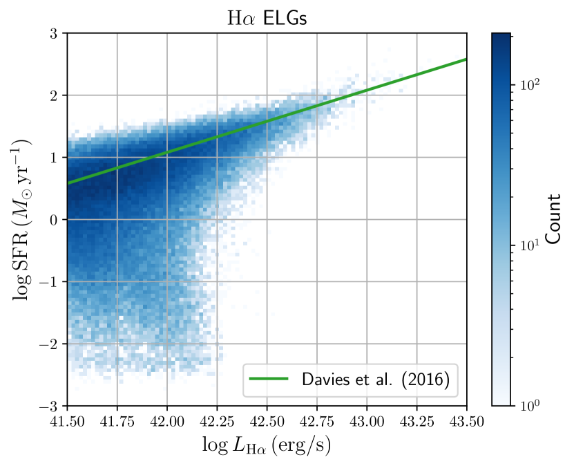
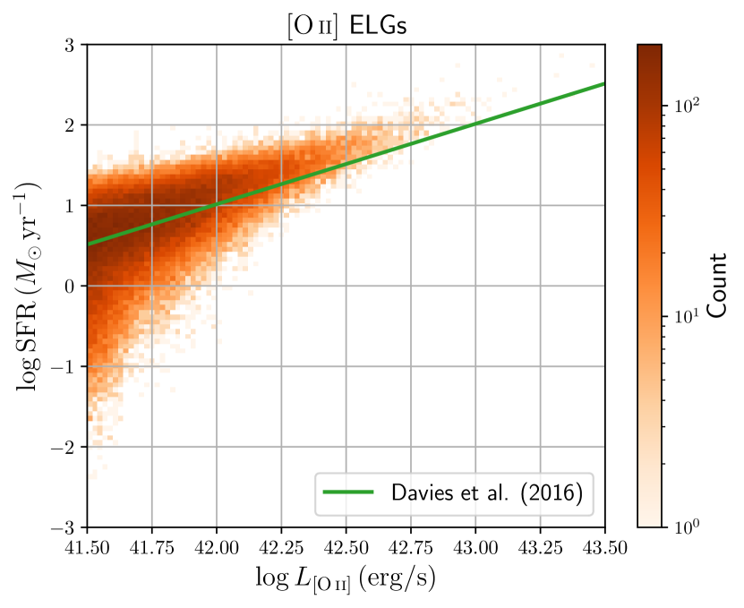
Figure 1: The SFR-line luminosity relation of H$\alpha$ ELGs (upper panel) and [O ii] ELGs (lower panel). For line luminosities, the dust attenuation effect has been considered. The power-law relations (Eqs. 18 and 19) based on observational estimates (Davies et al., 2016) are shown as green solid lines.

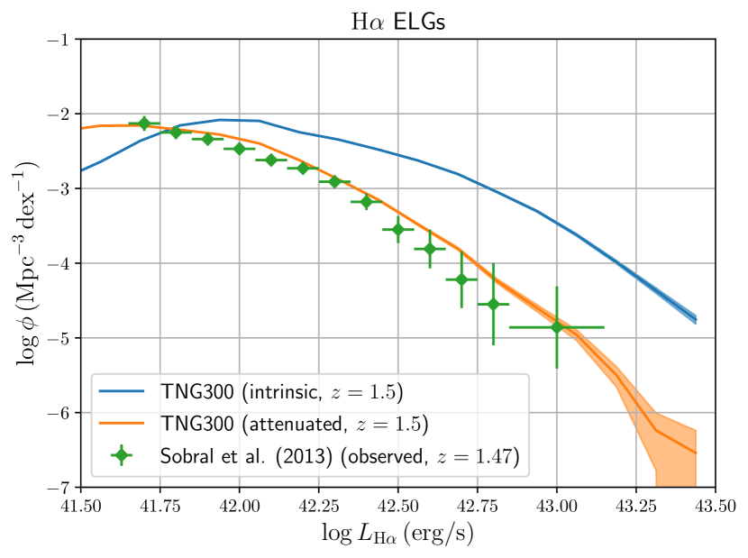
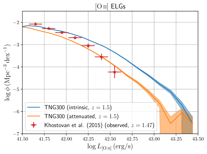
Figure 2: Luminosity functions of H$\alpha$ ELGs (upper panel) and [O ii] ELGs (lower panel). Orange solid lines show the results with the dust attenuation effect considered but blue solid lines correspond to the results of intrinsic luminosities, i.e., without dust attenuation. The error bars are determined as Poisson error. We also show the results of observations of Sobral et al. (2013) for H$\alpha$ ELGs and Khostovan et al. (2015) for [O ii] ELGs. Note that the values presented in Sobral et al. (2013) are after dust correction. We convert them to observed luminosities with the dust extinction magnitude $A_{\mathrm{H}\alpha}=1\,\mathrm{mag}$. The values in Khostovan et al. (2015) are before dust correction, and thus we use the raw values.

4.1 Galactic properties of ELGs

In order to verify our mock ELG catalogues, we compare galactic properties with observational estimates.

First, we measure the relation between star formation rate (SFR) and emission line luminosities. Since the nebular emission is driven by massive stars, the line luminosity is an indicator of star formation activity and the relation between SFR and line luminosities is well approximated with a power-law function (Kennicutt, 1998a). In hydrodynamical simulations, parameters related with star formation are calibrated so that the Kennicutt–Schmidt law (Kennicutt, 1998b) should be reproduced (Schaye & Dalla Vecchia, 2008; Pillepich et al., 2018a). In this sense, measuring the relation can be regarded as a sanity check of the mock ELG catalogues. In Figure 1, we show the SFR and H$\alpha$ and [O ii] line luminosity relations measured from mock ELG catalogues along with observational estimates from Davies et al. (2016) assuming the initial mass function of Chabrier (2003):

$$\mathrm{SFR}_{\text{H$\alpha$}}(M_{\sun}\,\mathrm{yr}^{-1}) =\frac{L_{\text{H$\alpha$}}}{8.30\times 10^{40}\,\mathrm{erg}\,\mathrm{s}^{-1}},$$ (18)

$$\mathrm{SFR}_{\text{[\text{O\,{ii}}]}}(M_{\sun}\,\mathrm{yr}^{-1}) =\frac{L_{\text{[\text{O\,{ii}}]}}}{9.67\times 10^{40}\,\mathrm{erg}\,\mathrm{s}^{-1}},$$ (19)

where $L_{\text{H$\alpha$}}$ and $L_{\text{[\text{O\,{ii}}]}}$ are H$\alpha$ and [O ii] line luminosities with dust attenuation effect considered, respectively. Though there are scatters at the faint end, line luminosities and SFR are in power-law relations and consistent with the result of Davies et al. (2016).

Next, we consider luminosity functions of ELGs. In Figure 2, we compare the luminosity functions of H$\alpha$ and [O ii] ELGs with the observations of Sobral et al. (2013) for H$\alpha$ ELGs and Khostovan et al. (2015) for [O ii] ELGs. Since the line luminosity is subject to dust extinction, to obtain consistent results with observations, we need to take into account the dust attenuation effect, which was described in Section 2.2. Otherwise, the luminosity function would be overestimated. After correcting the dust attenuation effect, the measured luminosity function is consistent with the observations within $0.5\,\mathrm{dex}$. Thus, we conclude our mock ELG catalogues are reliable at the reasonable level. The effect of resolution of the simulations for luminosity functions is addressed in Appendix A.

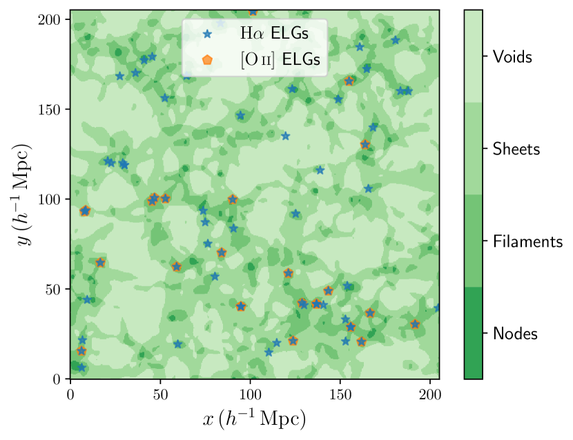
Figure 3: Classification of cosmic web structures for a slice of $0.40\,h^{-1}\,\mathrm{Mpc}$. The entire simulation volume is divided into four classes: nodes, filaments, sheets, and voids. The positions of H$\alpha$ and [O ii] ELGs are also shown as blue and orange symbols, respectively.

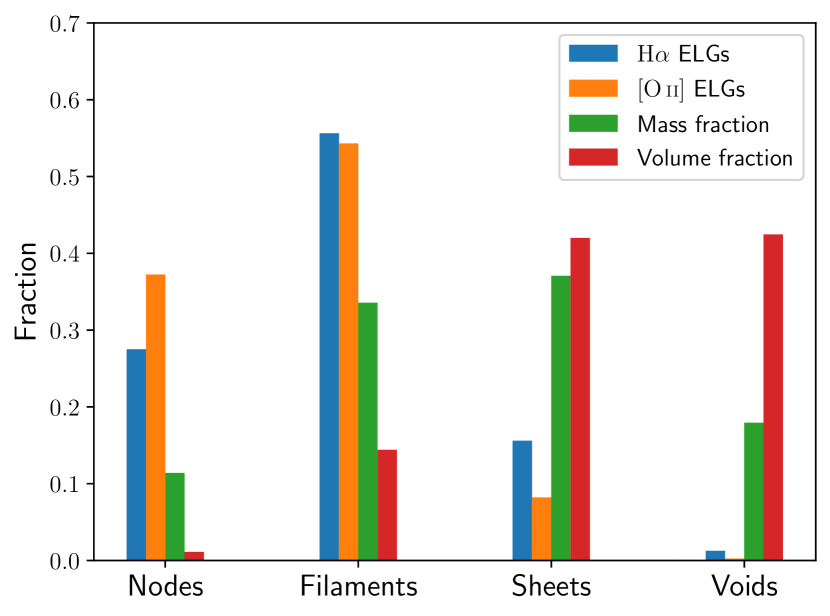
Figure 4: Fractions of H$\alpha$ and [O ii] ELGs with respect to the environments: nodes, filaments, sheets, and voids. For comparison, the mass and volume fractions are also shown.

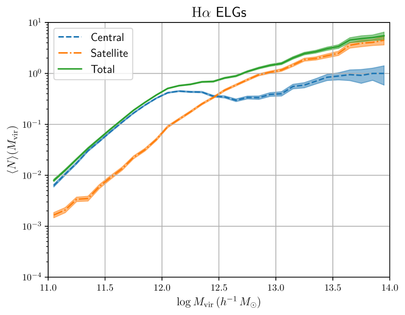
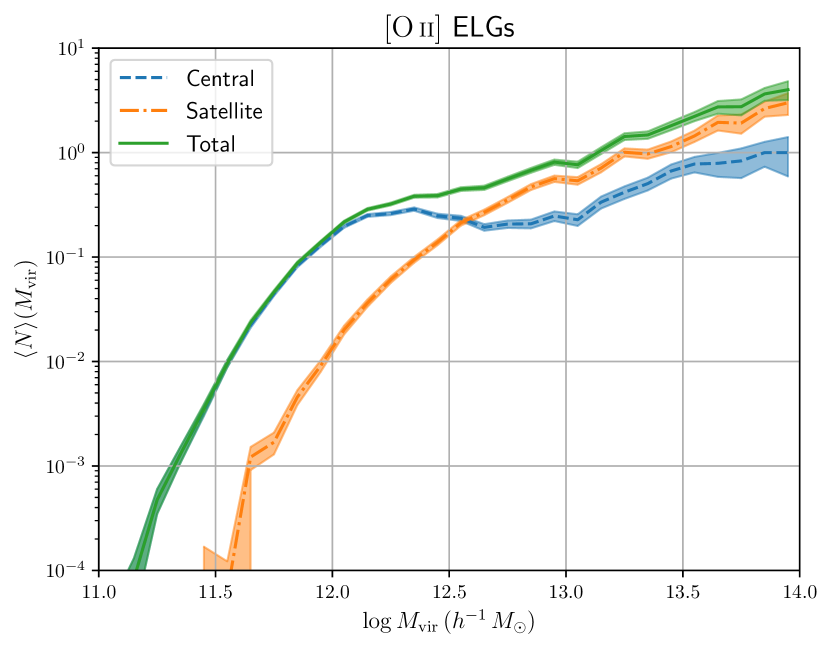
Figure 5: HODs of H$\alpha$ ELGs (upper panel) and [O ii] ELGs (lower panel) measured from simulations. Each ELG is classified as a central galaxy or a satellite galaxy based on whether the subhalo hosting the ELG is the subhalo or the host halo, which is derived with the SubFind algotirhm (Springel et al., 2001). HODs of central and satellite ELGs are also shown as separate dashed and dot-dashed lines, respectively. To construct ELG samples, the luminosity threshold ($L>10^{42}\,\mathrm{erg}\,\mathrm{s}^{-1}$) is applied, which corresponds to the number densiteis of $n_{\text{H$\alpha$}}=3.627\times 10^{-3}\,(h^{-1}\,\mathrm{Mpc})^{-3}$ and $n_{\text{[\text{O\,{ii}}]}}=1.277\times 10^{-3}\,(h^{-1}\,\mathrm{Mpc})^{-3}$ for H$\alpha$ and [O ii] ELGs, respectively. The shaded regions correspond to Poisson errors.

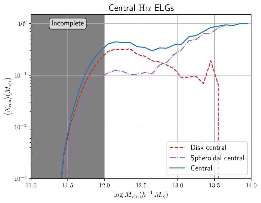
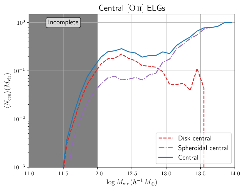
Figure 6: HODs of central H$\alpha$ ELGs (upper panel) and [O ii] ELGs (lower panel). The central ELGs are split into disk centrals and spheroidal centrals according to the bulge over total mass ratio. Since some of halos with masses $<10^{12}\,h^{-1}\,M_{\sun}$, which are displayed as grey regions in the figures, do not contain enough number of stellar particles to determine the bulge mass, and thus the total number of centrals at this mass range is incomplete.

4.2 Cosmic web environments around ELGs

Since ELGs are star-forming young populations, we expect that the majority of ELGs is infalling towards massive halos along filamentary structures (Gonzalez-Perez et al., 2020). We investigate where mock ELGs are found in terms of cosmic web structures (Hahn et al., 2007a, b; Cautun et al., 2014; Libeskind et al., 2018). First, we divide the entire simulation volume into four classes: nodes, filaments, sheets, and voids. For this purpose, we define the tidal tensor of the gravitational potential:

$$T_{ij}(\bm{x})\equiv\partialderivative{}{x_{i}}{x_{j}}\tilde{\phi}(\bm{x}),$$ (20)

where $\bm{x}$ is the comoving coordinates, $\tilde{\phi}(\bm{x})=\phi(\bm{x})/(4\pi G\bar{\rho}_{\mathrm{m}})$ is the normalized gravitational potential, $\phi(\bm{x})$ is the gravitational potential, $G$ is the gravitational constant, and $\bar{\rho}_{\mathrm{m}}$ is the mean matter density at the present Universe. The potential can be computed via the Poisson equation:

$$\nabla^{2}\tilde{\phi}(\bm{x})=\delta(\bm{x}),$$ (21)

where $\delta(\bm{x})$ is the density contrast. The density contrast is computed with regular grids by assigning matter particles with cloud-in-cell (CIC) algorithm. The number of grid is $512$ on a side and the corresponding grid size is $205\,h^{-1}\,\mathrm{Mpc}/512=0.40\,h^{-1}\,\mathrm{Mpc}$. In order to avoid small-scale transients, we apply Gaussian smoothing with the filter function:

$$W_{\mathrm{G}}(x)=\frac{1}{(2\pi\sigma_{\mathrm{G}})^{3/2}}\exp\left[-\frac{x^{2}}{2\sigma_{\mathrm{G}}^{2}}\right],$$ (22)

where the filtering scale is $\sigma_{\mathrm{G}}=2\,h^{-1}\,\mathrm{Mpc}$. Then, we deconvolve the aliasing effect due to CIC assignment (Jing, 2005). Next, we compute the eigenvalues of the tidal tensor for each position of regular grids, which are denoted as $(\lambda_{1},\lambda_{2},\lambda_{3})$ in an ascending order, and the position is classified according to the number of eigenvalues which exceed the threshold value $\lambda_{\mathrm{th}}$:

• Nodes: $\lambda_{\mathrm{th}}<\lambda_{1}<\lambda_{2}<\lambda_{3}$,

• Filaments: $\lambda_{1}<\lambda_{\mathrm{th}}<\lambda_{2}<\lambda_{3}$,

• Sheets: $\lambda_{1}<\lambda_{2}<\lambda_{\mathrm{th}}<\lambda_{3}$,

• Voids: $\lambda_{1}<\lambda_{2}<\lambda_{3}<\lambda_{\mathrm{th}}$.

We adopt the threshold value $\lambda_{\mathrm{th}}=0.2$, which reproduces the visual cosmic web structures (Forero-Romero et al., 2009). In Figure 3, we illustrate the cosmic web classification of the slice with the thickness of $0.40\,h^{-1}\,\mathrm{Mpc}$ together with the positions of H$\alpha$ and [O ii] ELGs. Here, ELGs are selected with the luminosity cut $L>10^{42}\,\mathrm{erg}\,\mathrm{s}^{-1}$. Visually, the distribution of ELGs traces the LSS, and most of ELGs are located at nodes or filaments and ELGs at voids are quite rare, which is consistent with the results of semi-analytic simulations (Gonzalez-Perez et al., 2020) and hydrodynamical simulations (Hadzhiyska et al., 2021). In Figure 4, we show the fractions of ELGs in terms of the four categories. The fractions for ELGs clearly show tendency different from mass and volume fractions. More than $50\%$ of ELGs are found in filaments, the rest is in nodes or sheets, and almost no ELGs are found in voids. The results indicate that a large fraction of ELGs is the population of infalling galaxies towards the gravitational potential well.

4.3 Halo occupation distribution of mock ELGs

Next, we measure the HODs of H$\alpha$ and [O ii] ELGs directly from simulations. Since the halo catalogues of IllustrisTNG simulations constructed with the SubFind algorithm (Springel et al., 2001) are provided, the information of mass and relation between host halos and subhalos is readily accessible. The most massive subhalo, which is located at the centre of the halo in most of cases, is labeled as a central galaxy and all the other subhalos are satellite galaxies. Figure 5 shows the measured HODs with the line luminosity cut $L>10^{42}\,\mathrm{erg}\,\mathrm{s}^{-1}$. In contrast to LRGs, the HOD of centrals cannot be well described by the step-like function but there are two components: a log-normal function which peaks around the mass of $10^{12}\,h^{-1}\,M_{\sun}$ and a step-like function which gradually reaches unity at the massive end. This overall feature is consistent with results of semi-analytic simulations (Gonzalez-Perez et al., 2018) and hydrodynamical simulations (Hadzhiyska et al., 2021), and both of the results also exhibit the peak of the central HOD at $10^{12}\,h^{-1}\,M_{\sun}$. Though the non-vanishing central HOD at the massive end is not incorporated in some HOD models for ELGs (see, e.g., Avila et al., 2020), the similar feature can be seen in semi-analytic simulations (Gonzalez-Perez et al., 2018). One of the possible reasons for the non-vanishing central HODs is that any magnitude cuts or colour selections (see, e.g., Raichoor et al., 2017) are not applied to construct our mock ELG catalogues and such selection may exclude central ELGs hosted by massive halos. The target selection of ELG candidates with our mock galaxy suite will be addressed in a future work.

Table 1: Range of HOD parameters adopted for the Zheng and Geach models.

Parameter	Range
Zheng HOD
$\sigma_{\log M}$, $\alpha$	$[0,\infty)$
$\log M_{\mathrm{min}}$, $\log M_{0}$, $\log M_{1}$	$[8,16]\,\log h^{-1}\,M_{\sun}$
Geach HOD
$F_{\mathrm{c}}$	$[0,1]$
$F_{\mathrm{s}}$, $\sigma_{\log M_{\mathrm{c1}}}$, $\sigma_{\log M_{\mathrm{c2}}}$, $\sigma_{\log M_{\mathrm{s}}}$, $\alpha$	$[0,\infty)$
$\log M_{\mathrm{c1}}$, $\log M_{\mathrm{c2}}$, $\log M_{\mathrm{s}}$	$[8,16]\,\log h^{-1}\,M_{\sun}$

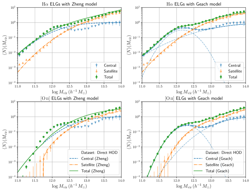
Figure 7: Best-fit HODs with the Zheng (left panels) and Geach (right panels) models for H$\alpha$ ELGs (upper panels) and [O ii] ELGs (lower panel). For the Geach model, the log-normal and step-like terms for central HODs are displayed as separate dashed lines.

In order to investigate the origin of the peak of the central HODs, in Gonzalez-Perez et al. (2018), the central ELGs are split into two populations, disk centrals and spheroidal centrals, based on a bulge over total mass ratio, and the former and latter corresponds to the log-normal and step-like function feature, respectively. The disk centrals undergo active star formation and are infalling towards the massive halos along filaments and considered as a majority of ELGs. On the other hand, spheroidal centrals are located close to the centre of the hosting halos and thus are expected to be quenched and not to be observed as ELGs. However, in the dense region such as the centre of halos, gas as fuel of star formation is replenished and star formation is kept active. Therefore, such spheroidal centrals are bright in the line emission. To verify this picture, we perform the analysis similar to that of Gonzalez-Perez et al. (2018) for our mock H$\alpha$ and [O ii] ELGs. Each stellar particle within a galaxy is classified as disk or bulge component according to the circularity parameter $\epsilon$ (Abadi et al., 2003). We make use of the supplementary catalogue of stellar circularity of Genel et al. (2015) and define the bulge mass fraction as the double of the fractional mass of stars with $\epsilon<0$. Then, if the bulge mass fraction is larger than $0.5$, the galaxy is classified as a “spheroidal galaxy” and otherwise as a “disk galaxy”. Figure 6 shows the central HODs of H$\alpha$ and [O ii] ELGs with central ELGs split into disk or spheroidal centrals. Though the decomposition is not possible for some of low mass halos ($M_{\mathrm{vir}}<10^{12}\,h^{-1}\,M_{\sun}$) due to the lack of the resolution, the transition from disk centrals to spheroidal centrals towards the massive end is clearly seen and the peak around $10^{12}\,h^{-1}\,M_{\sun}$ is dominated by disk centrals. This overall trend is consistent with the results of Gonzalez-Perez et al. (2018). For satellite HODs, previous studies (Geach et al., 2012; Contreras et al., 2013; Avila et al., 2020) suggest that the slope should be around $0.8\text{--}1$ but for our mock ELGs, a smaller slope ($\lesssim 0.7$) is preferred. That might indicate rapid quenching once ELGs infall to the halos in hydrodynamical simulations. Though these features are specific to our mock ELG catalogues, they appear at the massive end. Hence, the number of such massive halos is so small that the deviation does not have impacts on clustering statistics.

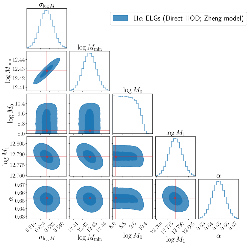
Figure 8: Constraints of HOD parameters for H$\alpha$ ELGs with the Zheng model by fitting the direct HOD. The thick (thin) blue regions correspond to $1\sigma$ ($2\sigma$) confidence level. The red lines indicate best-fit values. The unit of mass parameters ($M_{\mathrm{min}}$, $M_{0}$, $M_{1}$) is $h^{-1}\,M_{\sun}$.

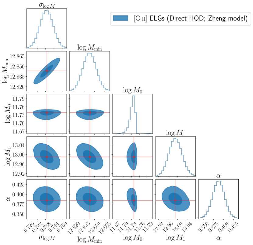
Figure 9: Same as Figure 8 but for [O ii] ELGs with the Zheng model.

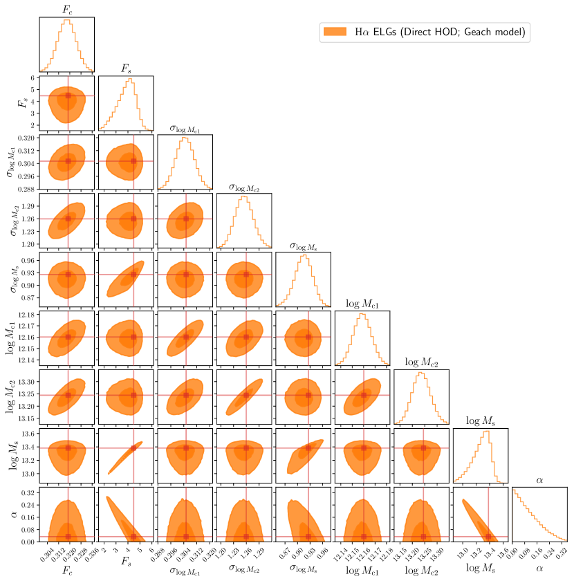
Figure 10: Same as Figure 8 but for H$\alpha$ ELGs with the Geach model. The unit of mass parameters ($M_{\mathrm{c1}}$, $M_{\mathrm{c2}}$, $M_{\mathrm{s}}$) is $h^{-1}\,M_{\sun}$.

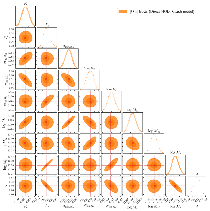
Figure 11: Same as Figure 8 but for [O ii] ELGs with the Geach model. The unit of mass parameters ($M_{\mathrm{c1}}$, $M_{\mathrm{c2}}$, $M_{\mathrm{s}}$) is $h^{-1}\,M_{\sun}$.

5 Inference of HOD parameters

5.1 Inference with direct HOD

In this section, we directly fit HOD parameters of the Zheng and Geach models with measured HODs and investigate which model fits the measured HODs well. In order to avoid the confusion of terminology, hereafter we refer to the HOD measured from simulations as “direct HOD” data set. Hereafter, the mock ELG sample consists of ELGs with the luminosity cut $L>10^{42}\,\mathrm{erg}\,\mathrm{s}^{-1}$, which is similar to the flux limit in the PFS survey. The resultant H$\alpha$ and [O ii] ELG number densities are $n_{\text{H$\alpha$}}=3.627\times 10^{-3}\,(h^{-1}\,\mathrm{Mpc})^{-3}$ and $n_{\text{[\text{O\,{ii}}]}}=1.277\times 10^{-3}\,(h^{-1}\,\mathrm{Mpc})^{-3}$, respectively. The likelihood of the direct HOD plus the ELG number density, $\mathcal{L}_{\mathrm{HOD}+n_{\mathrm{g}}}$, is given as

$$\log\mathcal{L}_{\mathrm{HOD}+n_{\mathrm{g}}} =-\frac{1}{2}\left(\chi^{2}_{\mathrm{cen}}+\chi^{2}_{\mathrm{sat}}+\chi^{2}_{n_{\mathrm{g}}}\right)+\text{const.},$$ (23)

$$\chi^{2}_{\mathrm{cen}} =\sum_{i}\frac{\left(\langle\hat{N}_{\mathrm{cen}}\rangle(M_{i})-\langle N_{\mathrm{cen}}\rangle(M_{i})\right)^{2}}{\sigma_{\mathrm{cen}}^{2}(M_{i})},$$ (24)

$$\chi^{2}_{\mathrm{sat}} =\sum_{i}\frac{\left(\langle\hat{N}_{\mathrm{sat}}\rangle(M_{i})-\langle N_{\mathrm{sat}}\rangle(M_{i})\right)^{2}}{\sigma_{\mathrm{sat}}^{2}(M_{i})},$$ (25)

$$\chi^{2}_{n_{\mathrm{g}}} =\frac{\left(\log_{10}\hat{n}_{\mathrm{g}}-\log_{10}n_{\mathrm{g}}\right)^{2}}{\sigma_{n_{\mathrm{g}}}^{2}},$$ (26)

where $\langle\hat{N}_{\mathrm{cen,sat}}\rangle$ is the measured mean occupation numbers of central or satellite ELGs, $\langle N_{\mathrm{cen,sat}}\rangle$ is the prediction based on the Geach or Zheng model, and we also include the chi-square of the number density $\chi^{2}_{n_{\mathrm{g}}}$; $\hat{n}_{\mathrm{g}}$ is the ELG number density measured in simulations and $n_{\mathrm{g}}$ is the expected number density (Eq. 14). We estimate the errors of the occupation numbers, $\sigma_{n_{\mathrm{cen}}}$ and $\sigma_{n_{\mathrm{cen}}}$, assuming the Poisson distribution. We set the error of the number density as $\sigma_{n_{\mathrm{g}}}=\tau|\log_{10}\hat{n}_{\mathrm{g}}|$ with $\tau=0.03$ (e.g., Okumura et al., 2021). The mass bin, which is labelled by the subscript $i$ in Eqs. (24) and (25), is logarithmically sampled in the range of $[10^{11},10^{14}]\,h^{-1}\,M_{\sun}$ with respect to virial mass with $30$ bins. We assume flat priors for all the HOD parameters and the considered parameter range is given in Table 1. Since the central HOD of the Geach model is not bounded to one, we also apply an additional prior that ensures the central HOD is less than one for any halo mass. In order to compute the posterior distribution, we employ Affine invariant Markov chain Monte-Carlo (MCMC) sampler emcee (Foreman-Mackey et al., 2013). Figure 7 shows the best-fitting HOD with the Zheng and Geach models and HOD parameter constraints are illustrated in Figures 8, 9, 10, and 11. In general, the Geach model outperforms the Zheng model in terms of fitting the measured HOD. The Zheng model can well fit the satellite HOD but fails to capture the two component feature of the central HOD. In contrast, the Geach model takes into account the characteristic nature of the central HOD by introducing the log-normal term and thus can explain the overall shape of the central HOD. It also should be noted that most of the HOD parameters are robustly determined and the marginalized posterior distributions are well approximated with normal distributions.

5.2 HOD challenge with projected correlation functions

In the real observations, HOD is not a direct observable but can be inferred from statistics of ELG clustering. The projected correlation function is widely used to constrain HOD models. We follow the procedure of the HOD parameter inference as in the practical measurements; we constrain model HOD parameters with the Bayesian inference procedure from the projected correlation function of mock ELGs. In Section 4.3, we have measured the HOD directly from the simulations. We thus can compare the HOD constrained from clustering statistics with those directly measured, namely the direct HOD. This analysis is a critical test for the HOD parameter inference and we refer to it as an HOD challenge.

The likelihood of the projected correlation function plus the ELG number density, $\mathcal{L}_{w_{\mathrm{p}}+n_{\mathrm{g}}}$, is given as

$$\log\mathcal{L}_{w_{\mathrm{p}}+n_{\mathrm{g}}}= -\frac{1}{2}\chi^{2}_{w_{\mathrm{p}}}-\frac{1}{2}\log\det\mathrm{Cov}[w_{\mathrm{p}}]-\frac{1}{2}\chi^{2}_{n_{\mathrm{g}}}+\text{const},$$ (27)

$$\chi^{2}_{w_{\mathrm{p}}}= \sum_{i,j}(\hat{w}_{\mathrm{p}}(R_{i})-\bar{w}_{\mathrm{p}}(R_{i}))\mathrm{Cov}^{-1}[w_{\mathrm{p}}](R_{i},R_{j})$$

$$\times(\hat{w}_{\mathrm{p}}(R_{j})-\bar{w}_{\mathrm{p}}(R_{j})),$$ (28)

where $\hat{w}_{\mathrm{p}}$ is the projected correlation function measured from the simulations, $\bar{w}_{\mathrm{p}}$ is the model prediction of the bin-averaged projected correlation functions (Eq. 9), and $\chi^{2}_{n_{\mathrm{g}}}$ is given in equation (26). Note that the covariance matrix has parameter dependence and thus the determinant of the covariance is no longer constant. We assume the same parameter range as that used in Section 5.1 (Table 1) and at every step of MCMC, we update the covariance matrix (Eq. 7). For the measurement of the projected correlation functions, we employ Corrfunc (Sinha & Garrison, 2020). The transverse bin is logarithmically sampled in the range of $[0.05,50]\,h^{-1}\,\mathrm{Mpc}$ with $15$ bins. This scale range is matched with the one employed in the measurement of the projected correlation function of [O ii] ELGs detected by Subaru HSC (Okumura et al., 2021). We will address how the parameter inference is affected by including the scale cut in Appendix B. Note that we do not correct integral constraint (Peebles & Groth, 1976) because the random correlation is analytically computed under the periodic boundary condition of the simulations and the effect is quite minor in the current setting. Similarly to the inference from the direct HOD, we employ emcee to compute the posterior distribution.

Figures 12, 13, 14, and 15 show HOD parameter constraints with the Zheng and Geach models from the projected correlation functions of H$\alpha$ and [O ii] ELGs. Though there are only 15 data points of the projected correlation function and 1 data point of galaxy number density, the HOD parameters are well constrained. On the other hand, several parameters, e.g., $M_{\mathrm{min}}$ for the Zheng model, exhibit multi-modal features, which were not seen in the direct HOD case. Figure 16 shows the best-fit projected correlation functions. With the help of many HOD parameters (5 for the Zheng model and 9 for the Geach model), both of the models can explain well the measured projected correlation function on all scales. On the other hand, the model predictions with best-fit parameters from direct HOD can reproduce the projected correlation functions only for scales $\gtrsim 1\,h^{-1}\,\mathrm{Mpc}$. The Geach model slightly outperforms the Zheng model as expected, since it fits the direct HOD better. The best-fitting Geach model works at the reasonable level though the non-linear effects cannot fully be captured. The results highlight that in the case of fitting of the projected correlation function, the advantage of the Geach model over the Zheng model is not so clear as in direct HOD inference and the performance of both of the HOD models looks quite similar. This fact is also indicated in the observations of Okumura et al. (2021). Figure 17 illustrates the HODs inferred from the projected correlation functions. Clearly, the best-fit HODs deviate from the measured HODs. For the Zheng model, central HOD is a sharp step-like function and the slope of the satellite HOD is close to zero. For the Geach model, the similar feature is observed and for central HODs, steep log-normal contribution is preferred. Thus, we can conclude that both of the Zheng and Geach models can explain the observed projected correlation functions but both of the models fail to reproduce the underlying HODs. In order to correctly reproduce the HODs, prior knowledge from simulations about the shape of HODs is essential.

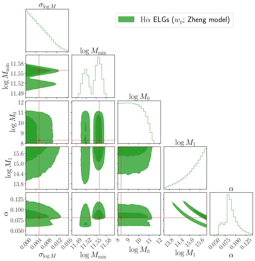
Figure 12: HOD parameter constraints with the Zheng HOD model from the projected correlation functions of H$\alpha$ ELGs. The thick (thin) green regions correspond to $1\sigma$ ($2\sigma$) confidence level. The red lines indicate best-fit values. The unit of mass parameters ($M_{\mathrm{min}}$, $M_{0}$, $M_{1}$) is $h^{-1}\,M_{\sun}$.

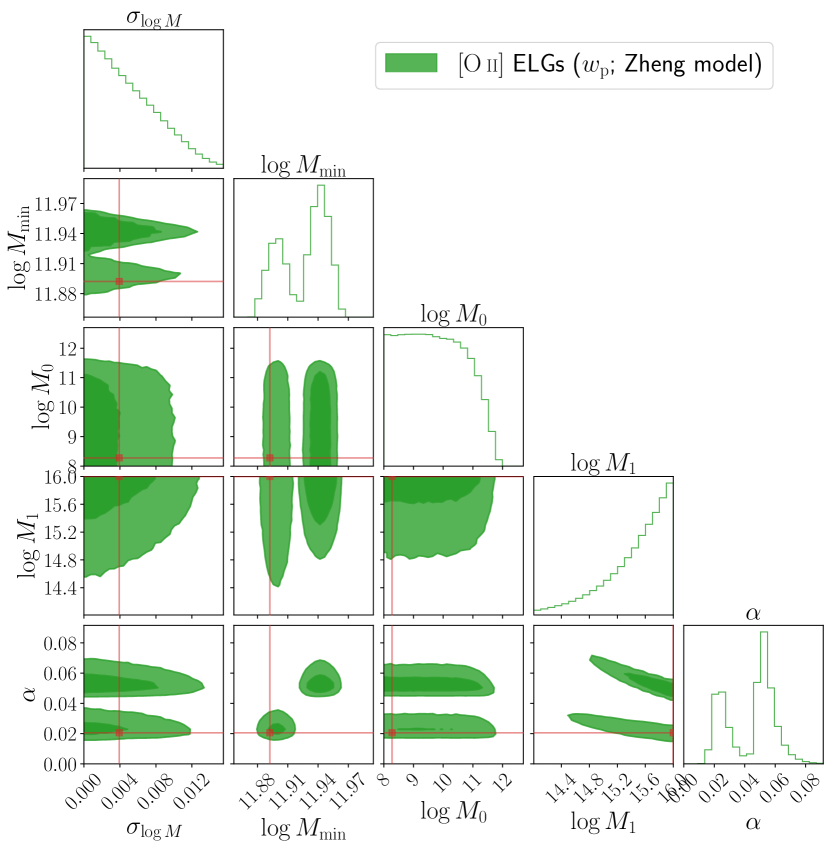
Figure 13: Same as Figure 12 but for [O ii] ELGs with the Zheng HOD model.

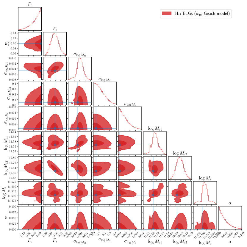
Figure 14: Same as Figure 12 but for H$\alpha$ ELGs with the Geach HOD model. The unit of mass parameters ($M_{\mathrm{c1}}$, $M_{\mathrm{c2}}$, $M_{\mathrm{s}}$) is $h^{-1}\,M_{\sun}$.

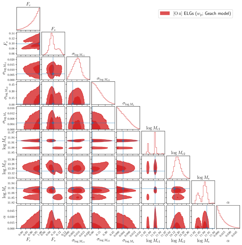
Figure 15: Same as Figure 12 but for [O ii] ELGs with the Geach HOD model. The unit of mass parameters ($M_{\mathrm{c1}}$, $M_{\mathrm{c2}}$, $M_{\mathrm{s}}$) is $h^{-1}\,M_{\sun}$.

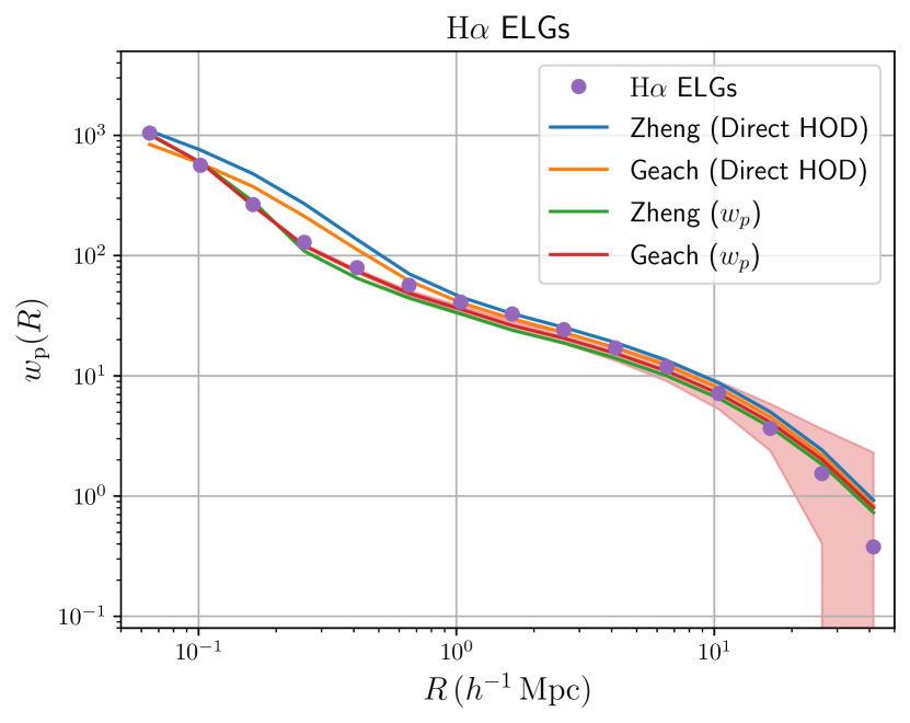
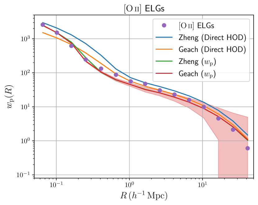
Figure 16: The projected correlation functions of H$\alpha$ ELGs (upper panel) and [O ii] ELGs (lower panel). The results of the best-fitting direct HOD and best-fitting projected correlation functions with the Zheng and Geach models are also shown as solid lines. The shaded regions correspond to standard deviation derived from the covariance matrix with best-fit HOD parameters. For visual reason, we only show the error of the result of best-fitting projected correlation functions with the Geach model.

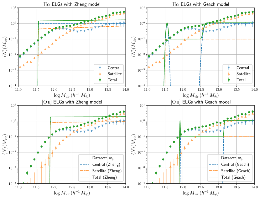
Figure 17: Best-fit HODs inferred from the projected correlation functions of H$\alpha$ ELGs (upper panels) and [O ii] ELGs (lower panels) with the Zheng (left panels) and Geach (right panels) models. For comparison, the HODs measured from simulations, i.e., direct HOD, are also shown as points.

5.3 Summary of best-fit parameters and goodness of fit

We have carried out parameter inference analyses with direct HOD and projected correlation functions. Here, we summarise the best-fit HOD parameters and derived parameters from the analyses.

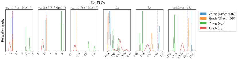
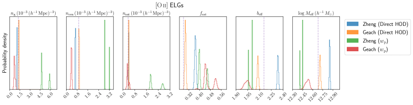
Figure 18: The one-dimensional posterior distributions of derived parameters: the galaxy number density $n_{\mathrm{g}}$, the central galaxy number density $n_{\mathrm{cen}}$, the satellite galaxy number density $n_{\mathrm{sat}}$, the satellite fraction $f_{\mathrm{sat}}$, the effective bias $b_{\mathrm{eff}}$, and the effective mass $M_{\mathrm{eff}}$. The purple dashed lines show the values measured directly from simulations.

Tables 2 and 3 summarise the best-fit HOD parameters from direct HOD and projected correlation functions. Note that the survey volume, which is matched to simulation volume $8.6\times 10^{6}\,(h^{-1}\,\mathrm{Mpc})^{3}$, is not so large compared with current and forthcoming spectroscopic surveys, and thus, the covariance is larger than the practical observations. Therefore, the current analysis leads to the conservative constraints on the parameters. Table 4 compares the derived parameters with best-fit HOD models with the values measured from simulations. Figure 18 shows one-dimensional histograms for derived parameters. The galaxy number densities of central and satellite and satellite fractions are computed directly from the mock ELG catalogues. The effective mass $M_{\mathrm{eff}}$ is calculated as the mean halo mass weighted with number of hosted ELGs. The effective bias $b_{\mathrm{eff}}$ can be computed in a similar manner with the halo bias fitting formula (Tinker et al., 2010). The general trend is that for direct HOD, the estimates with the Geach model are closer to simulations than the Zheng model. However, in the case of projected correlation functions, both of the models cannot reproduce the simulations values as these models fail to reconstruct the HOD as well. It should be noted that the derived parameters with the best-fitting models for projected correlation functions considerably deviate from the values measured directly from simulations. In particular, though the best-fitting Zheng model fits the projected correlation function very well, the number density is completely inconsistent with the true value directly measured from simulations. Therefore, even best-fitting models lead to biased estimates of derived parameters.

Compared with forecasts for upcoming surveys, the number density of our mock ELGs is higher, e.g., the forecast of the number density of [O ii] ELGs with PFS based on COSMOS Mock Catalogue (Jouvel et al., 2009) is $n_{\mathrm{g}}=5.5\times 10^{-4}\,(h^{-1}\,\mathrm{Mpc})^{-3}$ at the redshift $1.4<z<1.6$ with the flux limit $f>5\times 10^{-17}\,\mathrm{erg}\,\mathrm{s}^{-1}\,\mathrm{cm}^{-2}$ whereas for our mock [O ii] ELGs, the number density is $n_{\mathrm{g}}=1.3\times 10^{-3}(h^{-1}\,\mathrm{Mpc})^{-3}$ with the flux limit $f>6.7\times 10^{-17}\,\mathrm{erg}\,\mathrm{s}^{-1}\,\mathrm{cm}^{-2}$ derived from the luminosity threshold $L>10^{42}\,\mathrm{erg}\,\mathrm{s}^{-1}$ at the redshift $z=1.5$. The main reason for this overestimate is that no magnitude cut is applied for our mock ELG catalogues, but in reality, multiple magnitude or colour cuts are applied in target selection. Since our simulation pipeline also computes broad band magnitudes, it is possible to apply such magnitude cuts to mock ELGs and simulate target selection (Hadzhiyska et al., 2021). Though it is beyond the scope of this paper, the realistic target selection will be addressed in a future study. In terms of the satellite fraction, the satellite fractions for both of H$\alpha$ and [O ii] ELGs are $f_{\mathrm{sat}}\simeq 28\%$, i.e., the majority of ELGs is central and is likely to be hosted by isolated halos. Yuan et al. (2022) found that the satellite fraction is $33\%$ for the fiducial HOD model based on hydrodynamical simulations and Avila et al. (2020) estimated the satellite fraction as $22\%$ for the best-fit HOD model based on mock simulations designed for eBOSS. Though there are some scatters depending on assumed HOD models, the satellite fractions estimated from our mock ELGs are consistent with previous studies.

Table 2: Inferred HOD parameters for the Zheng model. The central values are best-fit values and errors are standard deviations. Note that the posterior distribution of some parameters deviates from normal distribution or even displays multi-model feature. For such distributions, the errors should be interpreted with cares.

Data	$\sigma_{\log M}$	$\log M_{\mathrm{min}}\,(h^{-1}\,M_{\sun})$	$\log M_{0}\,(h^{-1}\,M_{\sun})$	$\log M_{1}\,(h^{-1}\,M_{\sun})$	$\alpha$
H$\alpha$ ELGs
Direct HOD	$0.8296\pm 0.0058$	$12.428\pm 0.007$	$8.240\pm 0.676$	$12.786\pm 0.009$	$0.653\pm 0.008$
$w_{\mathrm{p}}$	$0.0052\pm 0.0038$	$11.560\pm 0.022$	$8.314\pm 0.884$	$16.000\pm 0.593$	$0.081\pm 0.017$
[O ii] ELGs
Direct HOD	$0.7389\pm 0.0048$	$12.843\pm 0.010$	$11.739\pm 0.024$	$12.990\pm 0.028$	$0.384\pm 0.017$
$w_{\mathrm{p}}$	$0.0039\pm 0.0036$	$11.892\pm 0.023$	$8.277\pm 1.004$	$15.999\pm 0.480$	$0.021\pm 0.016$

Table 3: Inferred HOD parameters for the Geach model. The central values are best-fit values and errors are standard deviations. Since the caveat about errors also holds here, see the caption of Table 2.

Data	$F_{\mathrm{c}}$	$F_{\mathrm{s}}$	$\sigma_{\log M_{\mathrm{c1}}}$	$\sigma_{\log M_{\mathrm{c2}}}$	$\sigma_{\log M_{\mathrm{s}}}$
H$\alpha$ ELGs
Direct HOD	$0.319\pm 0.007$	$4.479\pm 0.766$	$0.3054\pm 0.0057$	$1.2598\pm 0.0216$	$0.9258\pm 0.0219$
$w_{\mathrm{p}}$	$0.995\pm 0.085$	$0.099\pm 0.015$	$0.0211\pm 0.0057$	$0.0498\pm 0.1001$	$0.0020\pm 0.0078$
[O ii] ELGs
Direct HOD	$0.261\pm 0.009$	$0.194\pm 0.032$	$0.2856\pm 0.0049$	$0.7271\pm 0.0633$	$0.4195\pm 0.0184$
$w_{\mathrm{p}}$	$0.997\pm 0.059$	$0.098\pm 0.015$	$0.0059\pm 0.0042$	$0.0163\pm 0.1204$	$0.0048\pm 0.0040$

	$\log M_{\mathrm{c1}}\,(h^{-1}\,M_{\sun})$	$\log M_{\mathrm{c2}}\,(h^{-1}\,M_{\sun})$	$\log M_{\mathrm{s}}\,(h^{-1}\,M_{\sun})$	$\alpha$
H$\alpha$ ELGs
Direct HOD	$12.160\pm 0.008$	$13.245\pm 0.037$	$13.382\pm 0.136$	$0.034\pm 0.083$
$w_{\mathrm{p}}$	$11.558\pm 0.024$	$12.589\pm 0.061$	$11.504\pm 0.021$	$0.001\pm 0.025$
[O ii] ELGs
Direct HOD	$12.288\pm 0.012$	$13.356\pm 0.033$	$12.346\pm 0.038$	$0.722\pm 0.047$
$w_{\mathrm{p}}$	$11.920\pm 0.023$	$13.155\pm 0.066$	$11.906\pm 0.024$	$0.000\pm 0.014$

Table 4: Derived parameters inferred from the direct HOD and the projected correlation functions with the Zheng and Geach models. The central values are best-fit values and errors are standard deviations. Since the caveat about errors also holds here, see the caption of Table 2.

	$n_{\mathrm{g}}$	$n_{\mathrm{cen}}$	$n_{\mathrm{sat}}$	$f_{\mathrm{sat}}$	$b_{\mathrm{eff}}$	$\log M_{\mathrm{eff}}$
Unit	$10^{-3}\,(h^{-1}\,\mathrm{Mpc})^{-3}$	$10^{-3}\,(h^{-1}\,\mathrm{Mpc})^{-3}$	$10^{-3}\,(h^{-1}\,\mathrm{Mpc})^{-3}$	—	—	$h^{-1}\,M_{\sun}$
H$\alpha$ ELGs
Simulation	$3.627$	$2.599$	$1.028$	$0.283$	$1.858$	$12.490$
Zheng (direct HOD)	$3.590\pm 0.022$	$2.521\pm 0.019$	$1.069\pm 0.012$	$0.298\pm 0.003$	$1.883\pm 0.004$	$12.601\pm 0.004$
Geach (direct HOD)	$3.773\pm 0.027$	$2.698\pm 0.024$	$1.074\pm 0.012$	$0.285\pm 0.003$	$1.791\pm 0.006$	$12.508\pm 0.006$
Zheng ($w_{\mathrm{p}}$)	$11.284\pm 0.986$	$7.678\pm 0.404$	$3.606\pm 0.584$	$0.320\pm 0.020$	$1.677\pm 0.015$	$12.150\pm 0.016$
Geach ($w_{\mathrm{p}}$)	$2.272\pm 0.341$	$1.430\pm 0.205$	$0.842\pm 0.152$	$0.371\pm 0.023$	$1.755\pm 0.017$	$12.369\pm 0.026$
[O ii] ELGs
Simulation	$1.277$	$0.919$	$0.358$	$0.280$	$2.157$	$12.680$
Zheng (direct HOD)	$1.055\pm 0.013$	$0.666\pm 0.011$	$0.389\pm 0.007$	$0.369\pm 0.006$	$2.333\pm 0.007$	$12.852\pm 0.005$
Geach (direct HOD)	$1.338\pm 0.013$	$0.945\pm 0.011$	$0.393\pm 0.007$	$0.294\pm 0.004$	$2.077\pm 0.008$	$12.706\pm 0.009$
Zheng ($w_{\mathrm{p}}$)	$5.896\pm 0.572$	$3.210\pm 0.172$	$2.687\pm 0.401$	$0.456\pm 0.029$	$1.960\pm 0.023$	$12.409\pm 0.019$
Geach ($w_{\mathrm{p}}$)	$0.723\pm 0.093$	$0.407\pm 0.033$	$0.316\pm 0.068$	$0.437\pm 0.038$	$1.955\pm 0.029$	$12.539\pm 0.032$

To discuss the goodness of fit, Tables 5 and 6 summarise the chi-squares with best-fit HOD parameters for inferences from direct HOD and projected correlation functions. For direct HOD cases, the chi-square of the Geach model is much better than the Zheng model as is clear from visual impression. For projected correlation function cases, the fitting with the Geach model is slightly better than the Zheng model but the advantage of the Geach model is not manifest. Due to the large number of HOD parameters, both of models can fit the projected correlation functions, which in fact exhibit the monotonic shape for our fitting range. If data points at smaller scales, where the transition from two-halo term to one-halo term occurs, are included, the Zheng and Geach models can be distinguishable more clearly.

Table 5: The chi-squares with best-fit HOD parameters from the direct HOD. The number of data points is $N_{\mathrm{data}}=30+30+1=61$, the number of parameters is $N_{\mathrm{params}}=5$ for the Zheng model and $N_{\mathrm{params}}=9$ for the Geach model, and the degree of freedom is $N_{\mathrm{dof}}=N_{\mathrm{data}}-N_{\mathrm{params}}=56$ for the Zheng model and $N_{\mathrm{dof}}=52$ for the Geach model.

	$\chi^{2}_{\mathrm{cen}}$	$\chi^{2}_{\mathrm{sat}}$	$\chi^{2}_{n_{\mathrm{g}}}$	$\chi^{2}_{\mathrm{total}}$	$\chi^{2}_{\mathrm{total}}/N_{\mathrm{dof}}$
H$\alpha$ ELGs
Zheng	$3035.055$	$155.406$	$0.004$	$3190.464$	$56.973$
Geach	$88.756$	$112.769$	$0.055$	$201.580$	$3.877$
[O ii] ELGs
Zheng	$3541.013$	$62.061$	$0.913$	$3603.987$	$64.357$
Geach	$16.428$	$22.932$	$0.054$	$39.414$	$0.758$

Table 6: The chi-squares with best-fit HOD parameters from the projected correlation functions. The number of data points is $N_{\mathrm{data}}=15+1=16$, the number of parameters is $N_{\mathrm{params}}=5$ for the Zheng model and $N_{\mathrm{params}}=9$ for the Geach model, and the degree of freedom is $N_{\mathrm{dof}}=N_{\mathrm{data}}-N_{\mathrm{params}}=11$ for the Zheng model and $N_{\mathrm{dof}}=7$ for the Geach model.

	$\chi^{2}_{w_{\mathrm{p}}}$	$\log\det\mathrm{Cov}$	$\chi^{2}_{n_{\mathrm{g}}}$	$\chi^{2}_{\mathrm{total}}$	$\chi^{2}_{\mathrm{total}}/N_{\mathrm{dof}}$
H$\alpha$ ELGs
Zheng	$258.802$	$22.983$	$45.328$	$327.113$	$29.738$
Geach	$116.691$	$23.442$	$7.693$	$147.826$	$21.118$
[O ii] ELGs
Zheng	$317.360$	$55.102$	$58.572$	$431.034$	$39.185$
Geach	$168.730$	$55.001$	$8.100$	$231.831$	$33.119$

6 Conclusions

Upcoming spectroscopic redshift surveys aim to measure the statistics of the galaxy distribution and constrain cosmological models at the unprecedented accuracy. In such upcoming surveys ELGs become the main target as a tracer of the large-scale matter distribution because they probe the deeper universe, $z\gtrsim 1$, where star formation is active. The formation and evolution processes of ELGs are, however, quite different from those of LRGs which have been employed in the past galaxy surveys. While LRGs are old and quenched galaxies, ELGs are blue and star-forming galaxies and thus are undergoing infall towards massive halos along the filamentary structures. This coherent dynamics has a considerable effect on modelling of galaxy clustering statistics. Therefore, it is critical and timely to address the galaxy-halo connection for ELGs.

In this study, we leverage the hydrodynamical simulations, where galaxy formation physics is implemented as the subgrid model. The state-of-the-art hydrodynamical simulations can reproduce a variety of observational results, e.g., stellar mass functions and stellar-to-halo mass relations. Therefore, the simulations enable us to generate realistic mock ELG catalogues. Among the latest galaxy formation simulations, we have employed IllustrisTNG simulations, which cover a large cosmological volume $(205\,h^{-1}\,\mathrm{Mpc})^{3}$ in comoving scale. With this simulation suite, we generate mock ELG catalogues of H$\alpha$ and [O ii] ELGs, which are targets of PFS and Euclid surveys, respectively, by post-processing the particle outputs and halo catalogues with stellar population synthesis code PÉGASE-3. Since IllustrisTNG simulations have information about the matter distributions and detailed halo catalogues, we can scrutinise the ELG-halo connections, which help us improve theoretical modelling of ELG clustering including the non-linear regime.

First we have focused on the basic properties of mock ELGs to validate our mock catalogues. Our mock ELG catalogues successfully reproduced the luminosity functions and SFR-line luminosity relations estimated from observations once the dust attenuation effect was considered. Next, we have measured the HODs, i.e., mean occupation number of ELGs as a function of host halo mass. It is known that the central ELGs are composed of two distinct components: infalling disk galaxies and bulge-dominated spheroidal galaxies. In particular, the former induce the peak in HODs of central HODs, which is well described as the log-normal distribution. This feature has been confirmed also from our mock ELG catalogues and the Geach model explained the shape of HODs better than the conventional Zheng model.

Then, we have carried out the inference analysis of HOD parameters using the HODs directly measured from the mock catalogues. As expected, the Geach model can fit the measured HODs better and reproduce the galaxy number density as well. The Zheng model has fewer parameters and cannot describe the specific shape of central HODs. We have also investigated the constraints of HOD parameters from the projected correlation functions, which are widely used as cosmological statistics of the ELG distribution. Both of the Zheng and Geach models can reproduce the measured correlation functions down to small scales ($\simeq 0.1\,h^{-1}\,\mathrm{Mpc}$). These models have many free parameters ($5$ and $9$ parameters for the Zheng and Geach models, respectively) and thus, the large degree of freedom helps to fit the entire shape of the projected correlation functions. The HODs with best-fit parameters are, however, appreciably different from the measured HODs. It is expected because the projected correlation functions entail only a part of information of ELG clustering.

In this paper, as Part I of the series, we have focused only on the projected correlation function, which is less subject to the velocity information of ELGs. The kinematics of ELG in host halos, e.g., infall motion, strongly affects the velocity statistics, which can be observed through redshift space distortions. In the forthcoming papers of this series, we will present a challenge analysis with three-dimensional ELG correlation functions in redshift space to constrain the growth rate. Then we will investigate the relationship between ELGs and host halos, paying particular attention to the velocity and assembly biases of ELGs. That will help us construct more reliable modelling of ELG clustering and enhance the capability of theoretical models to predict the cosmological statistics precisely.

Data Availability

The data underlying this article will be shared on reasonable request to the corresponding author. The simulation data of IllustrisTNG is available at https://www.tng-project.org/.

Appendix A Convergence with respect to resolution of hydrodynamical simulations

In order to address the effects of resolution of the simulations, we compare the results with TNG300, which is the fiducial simulation used in this work, and the higher resolution run TNG100-1, hereafter TNG100. For TNG100, the simulation box length on a side is $75\,h^{-1}\,\mathrm{Mpc}$ and the number of dark matter particle and gas cells is $1820^{3}$ for each. The resultant mass resolution is $5.1\times 10^{6}\,h^{-1}\,M_{\sun}$ for dark matter particle and $9.4\times 10^{5}\,h^{-1}\,M_{\sun}$ for gas cell. Figure 19 shows the luminosity functions of H$\alpha$ and [O ii] ELGs with TNG300 and TNG100. Overall, the results from these two simulations are consistent. Since TNG100 simulation can resolve faint ELGs, the luminosity functions without dust attenuation keep the power-law form down to $10^{41.5}\,\mathrm{erg}\,\mathrm{s}^{-1}$, where the sudden decrease appears for TNG300 due to the lack of resolution. In this work, we have applied luminosity threshold $L>10^{42}\,\mathrm{erg}\,\mathrm{s}^{-1}$ to define the ELG samples and we can conclude that the resolution convergence is well achieved.

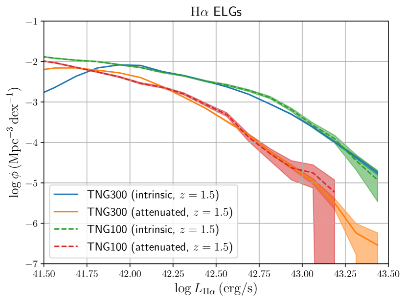
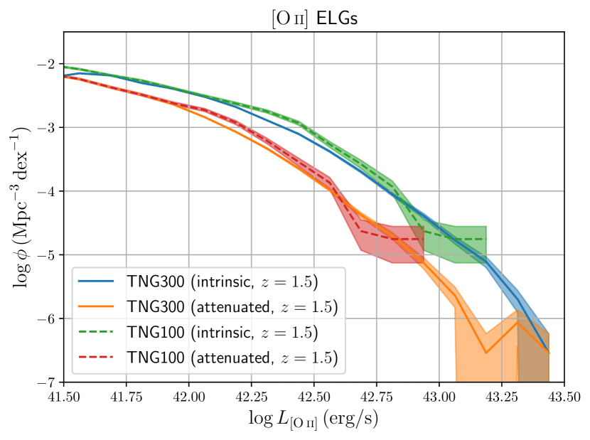
Figure 19: Luminosity functions of H$\alpha$ ELGs (upper panel) and [O ii] ELGs (lower panel) with TNG300 and TNG100. Orange and red solid lines show the results with the dust attenuation effect considered but blue and green solid lines correspond to the results of intrinsic luminosities. The error bars are determined as Poisson error.

Appendix B Effect of the scale cut for HOD parameter inference with the projected correlation function

While the theoretical prediction of the projected correlation function based on the halo model is less accurate at small scales, the error of the measurement at such scales becomes smaller. Thus, the parameter inference strongly depends on the small-scale data points and inferred parameters can be biased due to the low accuracy of the model. Here, we investigate how the small-scale data points affect the fitting of the projected correlation function. In order to address this effect, we have carry out the HOD parameter inference with the projected correlation functions with the scale cut which excludes two data points at $R=6.46\times 10^{-2}\,h^{-1}\,\mathrm{Mpc}$ and $1.01\times 10^{-1}\,h^{-1}\,\mathrm{Mpc}$. Since removing these data points leads to worse convergence of our MCMC analysis, we show only the best-fit correlation functions and HODs. Figure 20 shows the best-fit projected correlation functions with the scale cut. Clearly, the projected correlation functions can be reproduced well similarly to the case without the scale cut. Next, Figure 21 shows the best-fit HODs inferred from the projected correlation functions with the scale cut. The best-fit parameters for the Zheng and Geach models are summarized in Tables 7 and 8, respectively. The derived parameters and goodness-of-fit with the best-fit HOD parameters are respectively shown in Tables 9 and 10. The scale cut yields some improvements in reproducing true HODs and galaxy number densities directly measured in simulations. For example, for both H$\alpha$ and [O ii] ELGs, the peak locations of central HODs become closer to those of measured HODs than without the scale cut. However, the overall shape of HODs is still quite different from the measured HODs. Thus, our conclusion that HODs cannot be fully reproduced solely with the projected correlation functions holds even with the scale cut.

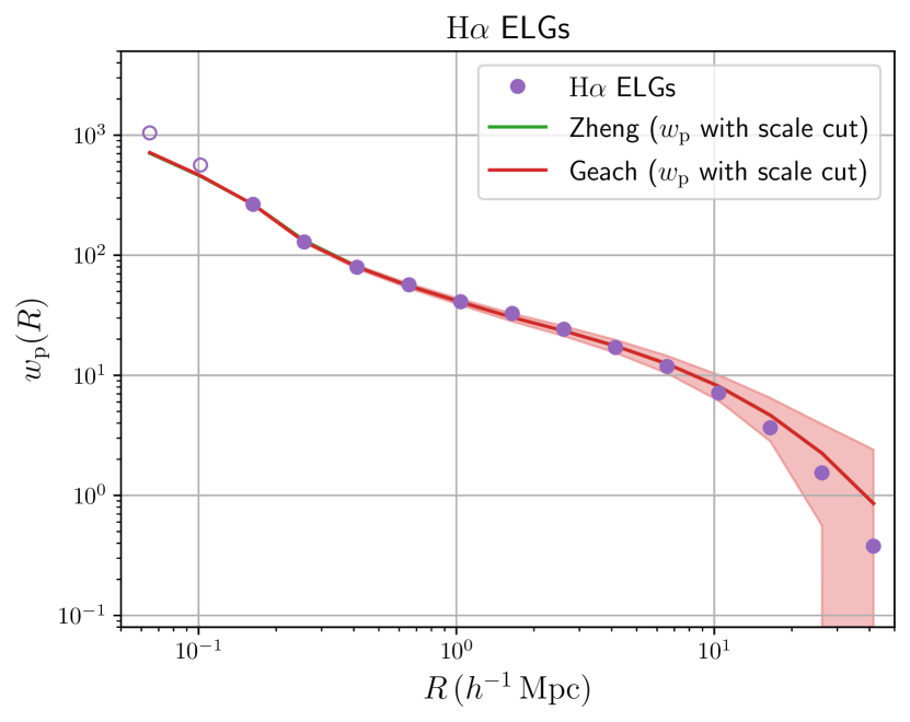
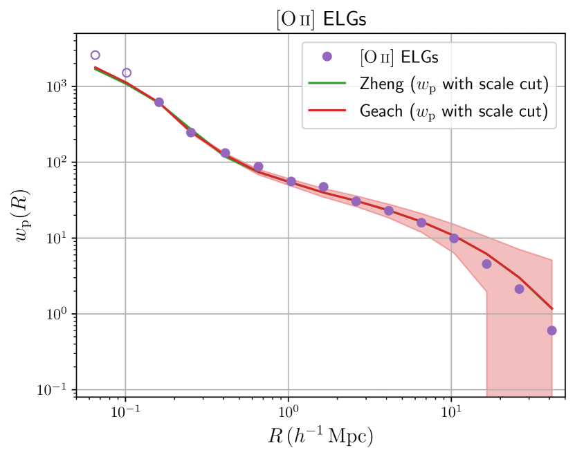
Figure 20: The projected correlation functions of H$\alpha$ ELGs (upper panel) and [O ii] ELGs (lower panel) with the scale cut. The shaded regions correspond to standard deviation derived from the covariance matrix with best-fit HOD parameters. For a visual reason, we only show the error of the result of best-fitting projected correlation functions with the Geach model. The open symbols correspond to the data points excluded in the analysis due to the scale cut.

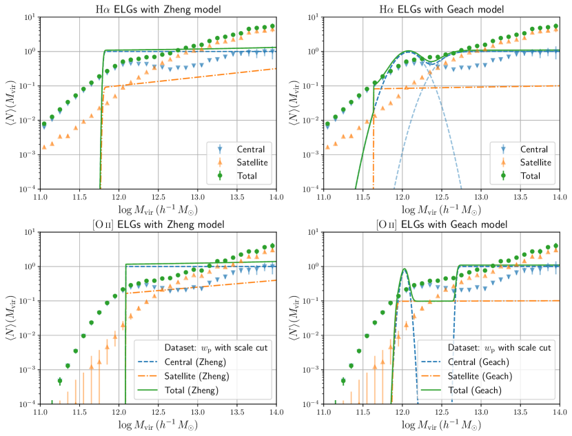
Figure 21: Best-fit HODs inferred from the projected correlation functions of H$\alpha$ ELGs (upper panels) and [O ii] ELGs (lower panels) with the scale cut with the Zheng (left panels) and Geach (right panels) models. For comparison, the HODs measured from simulations, i.e., direct HOD, are also shown as points.

Table 7: The best-fit HOD parameters inferred with the projected correlation functions with the scale cut for the Zheng model.

Data	$\sigma_{\log M}$	$\log M_{\mathrm{min}}\,(h^{-1}\,M_{\sun})$	$\log M_{0}\,(h^{-1}\,M_{\sun})$	$\log M_{1}\,(h^{-1}\,M_{\sun})$	$\alpha$
H$\alpha$ ELGs
$w_{\mathrm{p}}$ with scale cut	$0.0159$	$11.801$	$9.244$	$15.998$	$0.249$
[O ii] ELGs
$w_{\mathrm{p}}$ with scale cut	$0.0005$	$12.083$	$8.244$	$15.999$	$0.200$

Table 8: The best-fit HOD parameters inferred with the projected correlation functions with the scale cut for the Geach model.

Data	$F_{\mathrm{c}}$	$F_{\mathrm{s}}$	$\sigma_{\log M_{\mathrm{c1}}}$	$\sigma_{\log M_{\mathrm{c2}}}$	$\sigma_{\log M_{\mathrm{s}}}$	$\log M_{\mathrm{c1}}\,(h^{-1}\,M_{\sun})$	$\log M_{\mathrm{c2}}\,(h^{-1}\,M_{\sun})$	$\log M_{\mathrm{s}}\,(h^{-1}\,M_{\sun})$	$\alpha$
H$\alpha$ ELGs
$w_{\mathrm{p}}$ with scale cut	$0.956$	$0.082$	$0.1574$	$0.2204$	$0.0015$	$12.077$	$12.474$	$11.634$	$0.038$
[O ii] ELGs
$w_{\mathrm{p}}$ with scale cut	$0.767$	$0.098$	$0.0403$	$0.0238$	$0.0258$	$12.027$	$12.692$	$11.923$	$0.008$

Table 9: The best-fit derived parameters inferred with the projected correlation functions with the scale cut. For comparison, the results measured from simulations are also shown.

	$n_{\mathrm{g}}$	$n_{\mathrm{cen}}$	$n_{\mathrm{sat}}$	$f_{\mathrm{sat}}$	$b_{\mathrm{eff}}$	$\log M_{\mathrm{eff}}$
Unit	$10^{-3}\,(h^{-1}\,\mathrm{Mpc})^{-3}$	$10^{-3}\,(h^{-1}\,\mathrm{Mpc})^{-3}$	$10^{-3}\,(h^{-1}\,\mathrm{Mpc})^{-3}$	—	—	$h^{-1}\,M_{\sun}$
H$\alpha$ ELGs
Simulation	$3.627$	$2.599$	$1.028$	$0.283$	$1.858$	$12.490$
Zheng ($w_{\mathrm{p}}$ with scale cut)	$4.571$	$4.107$	$0.464$	$0.101$	$1.878$	$12.344$
Geach ($w_{\mathrm{p}}$ with scale cut)	$3.433$	$2.903$	$0.529$	$0.154$	$1.878$	$12.361$
[O ii] ELGs
Simulation	$1.277$	$0.919$	$0.358$	$0.280$	$2.157$	$12.680$
Zheng ($w_{\mathrm{p}}$ with scale cut)	$2.374$	$1.989$	$0.384$	$0.162$	$2.153$	$12.559$
Geach ($w_{\mathrm{p}}$ with scale cut)	$1.085$	$0.790$	$0.296$	$0.272$	$2.156$	$12.631$

Table 10: The chi-squares with best-fit HOD parameters from the projected correlation functions with the scale cut. The number of data points is $N_{\mathrm{data}}=13+1=14$, the number of parameters is $N_{\mathrm{params}}=5$ for the Zheng model and $N_{\mathrm{params}}=9$ for the Geach model, and the degree of freedom is $N_{\mathrm{dof}}=N_{\mathrm{data}}-N_{\mathrm{params}}=9$ for the Zheng model and $N_{\mathrm{dof}}=5$ for the Geach model.

	$\chi^{2}_{w_{\mathrm{p}}}$	$\log\det\mathrm{Cov}$	$\chi^{2}_{n_{\mathrm{g}}}$	$\chi^{2}_{\mathrm{total}}$	$\chi^{2}_{\mathrm{total}}/N_{\mathrm{dof}}$
H$\alpha$ ELGs
Zheng	$5.510$	$16.935$	$1.883$	$24.328$	$2.703$
Geach	$3.448$	$16.929$	$0.107$	$20.483$	$4.097$
[O ii] ELGs
Zheng	$27.149$	$43.332$	$9.621$	$80.102$	$8.900$
Geach	$8.955$	$43.366$	$0.661$	$52.982$	$10.596$

References

- Abadi et al. (2003) Abadi M. G., Navarro J. F., Steinmetz M., Eke V. R., 2003, ApJ, 597, 21
- Alam et al. (2021) Alam S., et al., 2021, Phys. Rev. D, 103, 083533
- Amendola et al. (2013) Amendola L., et al., 2013, Living Reviews in Relativity, 16, 6
- Aubourg et al. (2015) Aubourg É., et al., 2015, Phys. Rev. D, 92, 123516
- Avila et al. (2020) Avila S., et al., 2020, MNRAS, 499, 5486
- Berlind & Weinberg (2002) Berlind A. A., Weinberg D. H., 2002, ApJ, 575, 587
- Beutler et al. (2011) Beutler F., et al., 2011, MNRAS, 416, 3017
- Blake et al. (2011) Blake C., et al., 2011, MNRAS, 418, 1707
- Bressan et al. (1993) Bressan A., Fagotto F., Bertelli G., Chiosi C., 1993, A&AS, 100, 647
- Bryan & Norman (1998) Bryan G. L., Norman M. L., 1998, ApJ, 495, 80
- Byler et al. (2017) Byler N., Dalcanton J. J., Conroy C., Johnson B. D., 2017, ApJ, 840, 44
- Cautun et al. (2014) Cautun M., van de Weygaert R., Jones B. J. T., Frenk C. S., 2014, MNRAS, 441, 2923
- Chabrier (2003) Chabrier G., 2003, PASP, 115, 763
- Charlot & Fall (2000) Charlot S., Fall S. M., 2000, ApJ, 539, 718
- Charlot & Longhetti (2001) Charlot S., Longhetti M., 2001, MNRAS, 323, 887
- Conroy et al. (2006) Conroy C., Wechsler R. H., Kravtsov A. V., 2006, ApJ, 647, 201
- Contreras et al. (2013) Contreras S., Baugh C. M., Norberg P., Padilla N., 2013, MNRAS, 432, 2717
- Cooray & Sheth (2002) Cooray A., Sheth R., 2002, Phys. Rep., 372, 1
- Croton et al. (2016) Croton D. J., et al., 2016, ApJS, 222, 22
- DESI Collaboration et al. (2016a) DESI Collaboration et al., 2016a, arXiv e-prints, p. arXiv:1611.00036
- DESI Collaboration et al. (2016b) DESI Collaboration et al., 2016b, arXiv e-prints, p. arXiv:1611.00037
- Davies et al. (2016) Davies L. J. M., et al., 2016, MNRAS, 461, 458
- Desjacques et al. (2018) Desjacques V., Jeong D., Schmidt F., 2018, Phys. Rep., 733, 1
- Eisenstein et al. (2001) Eisenstein D. J., et al., 2001, AJ, 122, 2267
- Eisenstein et al. (2005) Eisenstein D. J., et al., 2005, ApJ, 633, 560
- Fagotto et al. (1994a) Fagotto F., Bressan A., Bertelli G., Chiosi C., 1994a, A&AS, 104, 365
- Fagotto et al. (1994b) Fagotto F., Bressan A., Bertelli G., Chiosi C., 1994b, A&AS, 105, 29
- Fagotto et al. (1994c) Fagotto F., Bressan A., Bertelli G., Chiosi C., 1994c, A&AS, 105, 39
- Favole et al. (2020) Favole G., et al., 2020, MNRAS, 497, 5432
- Favole et al. (2022) Favole G., Montero-Dorta A. D., Artale M. C., Contreras S., Zehavi I., Xu X., 2022, MNRAS, 509, 1614
- Ferland et al. (2017) Ferland G. J., et al., 2017, Rev. Mex. Astron. Astrofis., 53, 385
- Fioc & Rocca-Volmerange (2019) Fioc M., Rocca-Volmerange B., 2019, A&A, 623, A143
- Foreman-Mackey et al. (2013) Foreman-Mackey D., Hogg D. W., Lang D., Goodman J., 2013, PASP, 125, 306
- Forero-Romero et al. (2009) Forero-Romero J. E., Hoffman Y., Gottlöber S., Klypin A., Yepes G., 2009, MNRAS, 396, 1815
- Gao et al. (2022) Gao H., Jing Y. P., Zheng Y., Xu K., 2022, ApJ, 928, 10
- Geach et al. (2008) Geach J. E., Smail I., Best P. N., Kurk J., Casali M., Ivison R. J., Coppin K., 2008, MNRAS, 388, 1473
- Geach et al. (2012) Geach J. E., Sobral D., Hickox R. C., Wake D. A., Smail I., Best P. N., Baugh C. M., Stott J. P., 2012, MNRAS, 426, 679
- Genel et al. (2015) Genel S., Fall S. M., Hernquist L., Vogelsberger M., Snyder G. F., Rodriguez-Gomez V., Sijacki D., Springel V., 2015, ApJ, 804, L40
- Girardi et al. (1996) Girardi L., Bressan A., Chiosi C., Bertelli G., Nasi E., 1996, A&AS, 117, 113
- Gonzalez-Perez et al. (2018) Gonzalez-Perez V., et al., 2018, MNRAS, 474, 4024
- Gonzalez-Perez et al. (2020) Gonzalez-Perez V., et al., 2020, MNRAS, 498, 1852
- Hadzhiyska et al. (2021) Hadzhiyska B., Tacchella S., Bose S., Eisenstein D. J., 2021, MNRAS, 502, 3599
- Hahn et al. (2007a) Hahn O., Porciani C., Carollo C. M., Dekel A., 2007a, MNRAS, 375, 489
- Hahn et al. (2007b) Hahn O., Carollo C. M., Porciani C., Dekel A., 2007b, MNRAS, 381, 41
- Hamilton (2000) Hamilton A. J. S., 2000, MNRAS, 312, 257
- Hikage et al. (2013) Hikage C., Mandelbaum R., Takada M., Spergel D. N., 2013, MNRAS, 435, 2345
- Jing (2005) Jing Y. P., 2005, ApJ, 620, 559
- Jing et al. (1998) Jing Y. P., Mo H. J., Börner G., 1998, ApJ, 494, 1
- Jouvel et al. (2009) Jouvel S., et al., 2009, A&A, 504, 359
- Kennicutt (1998a) Kennicutt Robert C. J., 1998a, ARA&A, 36, 189
- Kennicutt (1998b) Kennicutt Robert C. J., 1998b, ApJ, 498, 541
- Kewley et al. (2019) Kewley L. J., Nicholls D. C., Sutherland R. S., 2019, ARA&A, 57, 511
- Khostovan et al. (2015) Khostovan A. A., Sobral D., Mobasher B., Best P. N., Smail I., Stott J. P., Hemmati S., Nayyeri H., 2015, MNRAS, 452, 3948
- Klypin et al. (2016) Klypin A., Yepes G., Gottlöber S., Prada F., Heß S., 2016, MNRAS, 457, 4340
- Laureijs et al. (2011) Laureijs R., et al., 2011, arXiv e-prints, p. arXiv:1110.3193
- Libeskind et al. (2018) Libeskind N. I., et al., 2018, MNRAS, 473, 1195
- Ma & Fry (2000) Ma C.-P., Fry J. N., 2000, ApJ, 543, 503
- Marian et al. (2015) Marian L., Smith R. E., Angulo R. E., 2015, MNRAS, 451, 1418
- Marigo (2001) Marigo P., 2001, A&A, 370, 194
- Marinacci et al. (2018) Marinacci F., et al., 2018, MNRAS, 480, 5113
- Naiman et al. (2018) Naiman J. P., et al., 2018, MNRAS, 477, 1206
- Navarro et al. (1996) Navarro J. F., Frenk C. S., White S. D. M., 1996, ApJ, 462, 563
- Navarro et al. (1997) Navarro J. F., Frenk C. S., White S. D. M., 1997, ApJ, 490, 493
- Nelson et al. (2018) Nelson D., et al., 2018, MNRAS, 475, 624
- Nelson et al. (2019) Nelson D., et al., 2019, Computational Astrophysics and Cosmology, 6, 2
- Okada et al. (2016) Okada H., et al., 2016, PASJ, 68, 47
- Okumura et al. (2015) Okumura T., Hand N., Seljak U., Vlah Z., Desjacques V., 2015, Phys. Rev. D, 92, 103516
- Okumura et al. (2016) Okumura T., et al., 2016, PASJ, 68, 38
- Okumura et al. (2021) Okumura T., Hayashi M., Chiu I. N., Lin Y.-T., Osato K., Hsieh B.-C., Lin S.-C., 2021, PASJ, 73, 1186
- Orsi & Angulo (2018) Orsi Á. A., Angulo R. E., 2018, MNRAS, 475, 2530
- Park et al. (2015) Park K., Di Matteo T., Ho S., Croft R., Wilkins S. M., Feng Y., Khandai N., 2015, MNRAS, 454, 269
- Peacock & Smith (2000) Peacock J. A., Smith R. E., 2000, MNRAS, 318, 1144
- Peebles & Groth (1976) Peebles P. J. E., Groth E. J., 1976, A&A, 53, 131
- Pillepich et al. (2018a) Pillepich A., et al., 2018a, MNRAS, 473, 4077
- Pillepich et al. (2018b) Pillepich A., et al., 2018b, MNRAS, 475, 648
- Planck Collaboration et al. (2016) Planck Collaboration et al., 2016, A&A, 594, A13
- Portinari et al. (1998) Portinari L., Chiosi C., Bressan A., 1998, A&A, 334, 505
- Raichoor et al. (2017) Raichoor A., et al., 2017, MNRAS, 471, 3955
- Salim & Narayanan (2020) Salim S., Narayanan D., 2020, ARA&A, 58, 529
- Schaye & Dalla Vecchia (2008) Schaye J., Dalla Vecchia C., 2008, MNRAS, 383, 1210
- Scoccimarro et al. (2001) Scoccimarro R., Sheth R. K., Hui L., Jain B., 2001, ApJ, 546, 20
- Seljak (2000) Seljak U., 2000, MNRAS, 318, 203
- Shimizu et al. (2016) Shimizu I., Inoue A. K., Okamoto T., Yoshida N., 2016, MNRAS, 461, 3563
- Sinha & Garrison (2020) Sinha M., Garrison L. H., 2020, MNRAS, 491, 3022
- Smith et al. (2003) Smith R. E., et al., 2003, MNRAS, 341, 1311
- Sobral et al. (2010) Sobral D., Best P. N., Geach J. E., Smail I., Cirasuolo M., Garn T., Dalton G. B., Kurk J., 2010, MNRAS, 404, 1551
- Sobral et al. (2013) Sobral D., Smail I., Best P. N., Geach J. E., Matsuda Y., Stott J. P., Cirasuolo M., Kurk J., 2013, MNRAS, 428, 1128
- Somerville & Davé (2015) Somerville R. S., Davé R., 2015, ARA&A, 53, 51
- Springel (2010) Springel V., 2010, MNRAS, 401, 791
- Springel et al. (2001) Springel V., White S. D. M., Tormen G., Kauffmann G., 2001, MNRAS, 328, 726
- Springel et al. (2005) Springel V., et al., 2005, Nature, 435, 629
- Springel et al. (2018) Springel V., et al., 2018, MNRAS, 475, 676
- Takada et al. (2014) Takada M., et al., 2014, PASJ, 66, R1
- Takahashi et al. (2012) Takahashi R., Sato M., Nishimichi T., Taruya A., Oguri M., 2012, ApJ, 761, 152
- Tinker et al. (2008) Tinker J., Kravtsov A. V., Klypin A., Abazajian K., Warren M., Yepes G., Gottlöber S., Holz D. E., 2008, ApJ, 688, 709
- Tinker et al. (2010) Tinker J. L., Robertson B. E., Kravtsov A. V., Klypin A., Warren M. S., Yepes G., Gottlöber S., 2010, ApJ, 724, 878
- Tonegawa et al. (2015) Tonegawa M., et al., 2015, PASJ, 67, 81
- Vale & Ostriker (2004) Vale A., Ostriker J. P., 2004, MNRAS, 353, 189
- Weinberg et al. (2013) Weinberg D. H., Mortonson M. J., Eisenstein D. J., Hirata C., Riess A. G., Rozo E., 2013, Phys. Rep., 530, 87
- Weinberger et al. (2017) Weinberger R., et al., 2017, MNRAS, 465, 3291
- Westera et al. (2002) Westera P., Lejeune T., Buser R., Cuisinier F., Bruzual G., 2002, A&A, 381, 524
- White & Frenk (1991) White S. D. M., Frenk C. S., 1991, ApJ, 379, 52
- Yuan et al. (2022) Yuan S., Hadzhiyska B., Bose S., Eisenstein D. J., 2022, MNRAS, 512, 5793
- Zehavi et al. (2011) Zehavi I., et al., 2011, ApJ, 736, 59
- Zheng et al. (2005) Zheng Z., et al., 2005, ApJ, 633, 791
- de la Torre et al. (2017) de la Torre S., et al., 2017, A&A, 608, A44
- van den Bosch et al. (2013) van den Bosch F. C., More S., Cacciato M., Mo H., Yang X., 2013, MNRAS, 430, 725