How GNNs Facilitate CNNs in Mining Geometric Information from Large-Scale Medical Images

Abstract

Gigapixel medical images provide massive data, both morphological textures and spatial information, to be mined. Due to the large data scale in histology, deep learning methods play an increasingly significant role as feature extractors. Existing solutions heavily rely on convolutional neural networks (CNNs) for global pixel-level analysis, leaving the underlying local geometric structure such as the interaction between cells in the tumor microenvironment unexplored. The topological structure in medical images, as proven to be closely related to tumor evolution, can be well characterized by graphs. To obtain a more comprehensive representation for downstream oncology tasks, we propose a fusion framework for enhancing the global image-level representation captured by CNNs with the geometry of cell-level spatial information learned by graph neural networks (GNN). The fusion layer optimizes an integration between collaborative features of global images and cell graphs. Two fusion strategies have been developed: one with MLP which is simple but turns out efficient through fine-tuning, and the other with Transformer gains a champion in fusing multiple networks. We evaluate our fusion strategies on histology datasets curated from large patient cohorts of colorectal and gastric cancers for three biomarker prediction tasks. Both two models outperform plain CNNs or GNNs, reaching a consistent AUC improvement of more than 5% on various network backbones. The experimental results yield the necessity for combining image-level morphological features with cell spatial relations in medical image analysis. Codes are available at https://github.com/yiqings/HEGnnEnhanceCnn.

1 Introduction

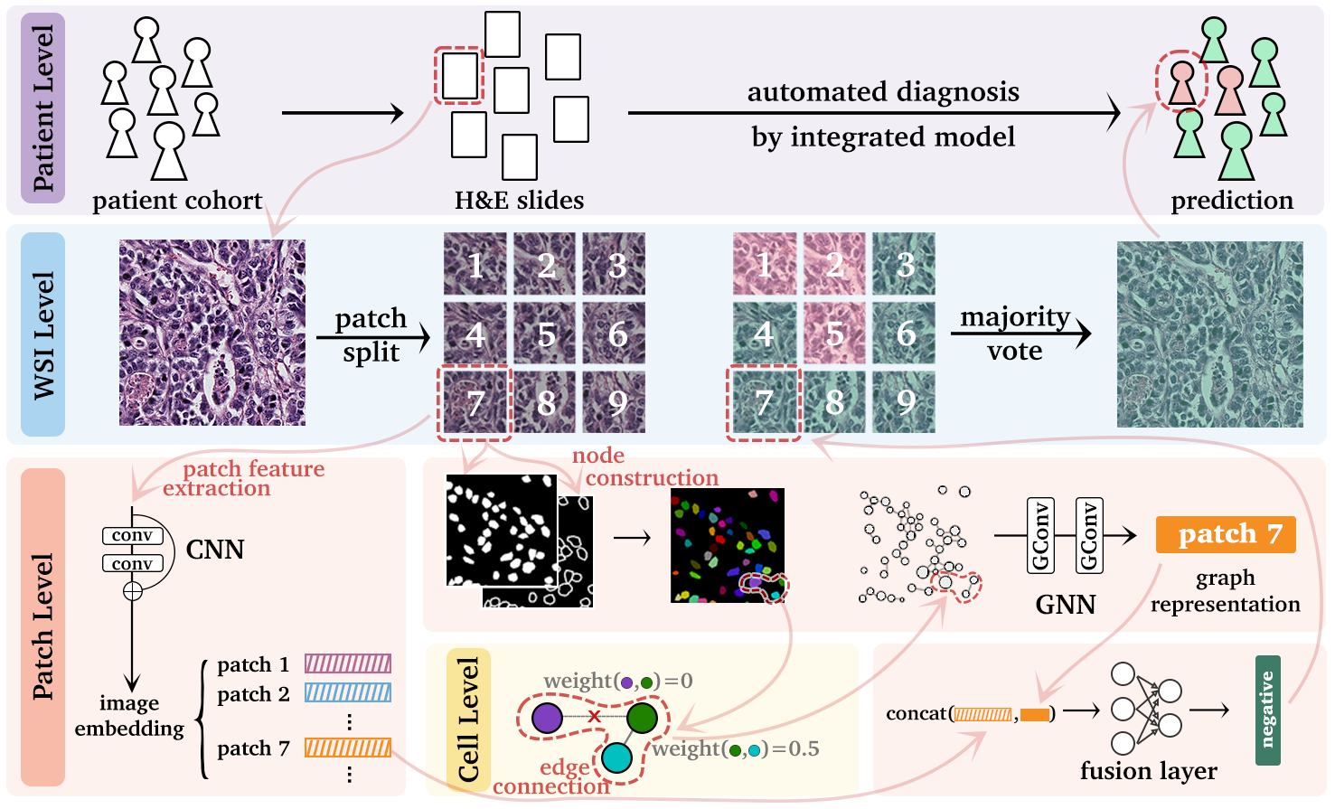
Figure 1: The use case of the proposed fusion scheme for GNN and CNN from histology whole-slide image in the patient-level diagnostic task. It consists of the following three steps. First, for each patches tessellated from WSI, a cell graph is generated to characterize the topological structures, where the nuclei region segmented by CA^2.5-Net are identified as graph nodes, with the node features extracted from the pre-defined pathomics. Then, in both the training and inference stage, the global image-level representation together with the geometric representation discovered by CNN and GNN, are integrated by a learnable fusion layer to obtain a more comprehensive feature representation. Finally, the patient-level prediction is determined by a majority vote from all patch predictions.

Large-scale medical images, such as histology, provide a wealth of complex patterns for deep learning algorithms to mine. Existing approaches routinely employ end-to-end convolutional neural networks (CNNs) frameworks, by taking the morphological and textural image features as input. Numerous practices with CNNs have been made in diagnostic and prognostic tasks, such as lesion detection, gene mutation identification, molecular biomarker classification, and patient survival analysis from Hematoxylin and Eosin (H&E) stained histology whole-slide images (WSIs) (Shaban et al., 2019; Fu et al., 2020; Liao et al., 2020; Calderaro and Kather, 2021; Echle et al., 2021a). Determined by the convolutional kernel which is primarily targeted to analyze fixed connectivity between local areas (i.e., pixel grids), CNNs focus on extracting global image-level feature representations. However, no guidance has been imposed explicitly on CNNs to exploit the underlying topological structures from input medical images, e.g., the cell-cell interaction and the spatial distribution of cells, which have been clinically proven to be closely related to tumor evolution and biomarker expression (Galon et al., 2006; Feichtenbeiner et al., 2014; Barua et al., 2018; Noble et al., 2022). The recognition of the cell dispersal manner and their mutual interactions are essential for training robust and interpretable deep learning models (Gunduz et al., 2004; Yener, 2016; Wang et al., 2021).

Mathematically, the topological structures and cell relationships are formulated by graphs. By its definition, a graph can characterize the relationship between nodes, e.g., super-pixels in natural images, or the cells in histological images. Following the establishment of graphs, graph neural networks (GNNs) were proposed to learn the geometric information (Bronstein et al., 2017; Wu et al., 2020; Zhang et al., 2020). While CNNs are capable of learning global image representation, GNNs can provide machinery for the local topological features. Both global and local features serve as significant representation in learning the mapping of histological image space to clinical meaningful biomarkers. One strategy is to make use of the own merits of CNN and GNN models. Some recent attempts at combining GNNs with CNNs have achieved satisfactory performance boost in natural image classification tasks, such as remote sensing scene recognition (Liang et al., 2020; Peng et al., 2022) and hyper-spectral image prediction (Dong et al., 2022). In the medical imaging domain, Wei et al. (2022) predicted isocitrate dehydrogenase gene mutation with a collaborative learning framework that aligns a CNN for tumor MRI with a GNN for tumor geometric shape analysis. To the best of our knowledge, a study of the interplay between CNNs and GNNs for histology is still absent.

In this paper, we develop an efficient strategy that is able to integrate the structure feature from GNNs with the image feature of CNNs for H&E slides analysis. The fusion scheme partitions a WSI into non-overlapped patches and generates a cell graph for each patch by linking associated cells (see Section 2) to model the cell interactions. Then, a GNN is employed to distill geometric representation. To fuse the graph-level representation learning with image-level embedding, we train the GNN together with the CNN in parallel. The integration takes place in a learnable fusion layer which incorporates the morphology feature of the whole image with the geometric representation of cell graphs. In this way, insights into the spatial structure are gained for a specific staining image, such as the distribution of cells, interaction of cancer and healthy cells, and tumor microenvironment.

In practice, we can simply connect a learnable fusion layer using MLP or Transformer next to the outputs of GNN and CNN modules. The simple amalgamation can produce a model which outperforms a sole GNN or CNN model on real histological image datasets (two public and one private). The key to performance improvement of the fusion model lies in that the local geometry of the cell graphs of patches which can only be perceived by GNNs tops up the global image feature of CNNs.

Contributions.

The contributions are three-fold: (1) We develop two fusion schemes, based on MLP and Transformer, for integrating the features extracted from CNNs and GNNs. Moreover, we present a use case of the proposed framework on histology analysis, where cell geometric behaviors are crucial for downstream diagnostics. (2) Experiments on three real-world and one synthetic datasets yield that geometric and image-level representations are complementary. (3) We release the constructed graph-image paired datasets, which can serve as a benchmark for future research in the image-graph bimodal domain.

2 Fusing CNN with GNN

Problem Formulation.

CNNs extract the global image-level representation ${\bm{H}}_{{\mathcal{I}}}$ from an input image ${\bm{X}}_{\mathcal{I}}$. However, the underlying geometric relationship, characterized by a graph $({\bm{X}}_{\mathcal{G}},{\bm{A}}_{\mathcal{G}})$ with node feature ${\bm{X}}_{\mathcal{G}}$ and adjacent matrix ${\bm{A}}_{\mathcal{G}}$, is not explicitly explored in CNN, although it is crucial for tasks such as medical imaging analysis. Therefore, we leverage a GNN to capture the geometric representation ${\bm{H}}_{{\mathcal{G}}}$ as an enhancement to ${\bm{H}}_{{\mathcal{I}}}$. The major scope of this paper is to construct a fusion scheme for the bimodal data $\big{(}{\bm{X}}_{\mathcal{I}},({\bm{X}}_{\mathcal{G}},{\bm{A}}_{\mathcal{G}})\big{)}$, especially in the medical domain.

2.1 Geometric Feature Representation

We denote the corresponded graph (e.g., cell graph in histology) to the image ${\bm{X}}_{\mathcal{I}}$ as ${\mathcal{G}}=({\mathcal{V}},{\mathcal{E}})$, where ${\mathcal{V}}$ is the collection of nodes, ${\mathcal{E}}$ is the set of all edges $e_{ij}$ with the attribute $w_{ij}$ describing the pair-wise node interaction. For notation simplicity, we use a matrix pair $({\bm{X}}_{\mathcal{G}},{\bm{A}}_{\mathcal{G}})$ to represents the node attributes and weighted edges, respectively. We name ${\bm{A}}_{\mathcal{G}}$ as an adjacency matrix with its element $({\bm{A}}_{\mathcal{G}})_{ij}=w_{ij}$. The $\ell$th layer of the GNN finds the hidden representation of the graph by

$${\bm{H}}^{\ell}_{{\mathcal{G}}}=\texttt{ReLU}\big{(}\texttt{GraphConv}\left({\bm{A}}_{\mathcal{G}},{\bm{H}}^{\ell-1}_{\mathcal{G}}\right)\big{)},$$ (1)

where ${\bm{H}}^{0}_{\mathcal{G}}={\bm{X}}_{\mathcal{G}}$. We consider spatial-based convolutions for GraphConv, which usually follow the message-passing (Gilmer et al., 2017) form. For the $i$th node of a graph, its representation ${\bm{H}}_{{\mathcal{G}},i}^{\ell}$ at the $\ell$th convolutional layer reads

$${\bm{H}}_{{\mathcal{G}},i}^{\ell}=\gamma\left({\bm{H}}_{{\mathcal{G}},i}^{\ell-1},\square_{j\in\mathcal{N}(i)}\phi({\bm{H}}^{\ell-1}_{{\mathcal{G}},i},{\bm{H}}^{\ell-1}_{{\mathcal{G}},j},{\bm{A}}_{ij})\right)$$ (2)

with some differentiable operators $\gamma$, $\phi$ (e.g., MLP) and permutation invariant aggregation function $\square$ (e.g., average or summation). The ${\bm{H}}^{\ell-1}_{{\mathcal{G}},j}$ denotes node $j$’s hidden representation at the $(\ell-1)$th layer, where $j\in{\mathcal{N}}(i)$ is a 1-hop neighbor of node $i$, i.e.,  ${\bm{A}}_{ij}={\bm{A}}_{ji}\neq 0$.

The representation ${\bm{H}}^{\ell}_{{\mathcal{G}}}$ embeds spatial topological structures of the underlying graph, which is usually sent to a readout layer, such as a linear layer, before eventually being fed into the fusion layer. We term this linear layer as the alignment layer, which helps to align the feature dimensions of the GNN with the parallel CNN output.

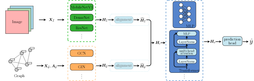
Figure 2: A schematic illustration for fusing the representations of local geometry and global image features. An image input ${\bm{X}}_{\mathcal{I}}$ is encoded to a global image-level presentation ${\bm{H}}_{\mathcal{I}}$ by CNNs. Meanwhile, the geometric information $({\bm{X}}_{\mathcal{G}},{\bm{A}}_{\mathcal{G}})$ from the image, which is first transformed into a cell graph with attributes, is embedded by GNNs (i.e., ${\bm{H}}_{\mathcal{G}}$). The two sets of hidden representation are then fed into a fusion layer for adaptive integration (i.e., ${\bm{H}}_{c}$). The output ${\bm{H}}_{o}$ is eventually send to a prediction head (e.g., classification or regression head) for training assignment.

2.2 Image-level Feature Representation

The image-level feature representation is directly extracted from histology patches by CNNs. For instance, denote $\{{\bm{H}}^{1}_{{\mathcal{I}}},\dots,{\bm{H}}^{\ell-1}_{{\mathcal{I}}}\}$ the output of the first $(\ell-1)$ blocks after convolution layers. We can use different convolutional module for the CNN. For example, a DenseNet (Huang et al., 2017) defines

$${\bm{H}}^{\ell}_{{\mathcal{I}}}=\texttt{ReLU}\big{(}\texttt{Conv}(\texttt{concat}[{\bm{H}}^{1}_{{\mathcal{I}}},\dots,{\bm{H}}^{\ell-1}_{{\mathcal{I}}}])\big{)}.$$ (3)

Alternatively, ResNet (He et al., 2016) finds ${\bm{H}}^{\ell}_{{\mathcal{I}}}$ by

$${\bm{H}}^{\ell}_{{\mathcal{I}}}=\texttt{ReLU}\big{(}\texttt{Conv}({\bm{H}}^{\ell-1})+{\bm{H}}^{\ell-1}\big{)}$$ (4)

with some activated convolutional layers $\texttt{Conv}(\cdot)$. The residual connection in the second design can reduce the computational cost of deep CNNs and circumvent gradient diminishing. In the empirical study, a lightweight architecture namely MobileNetV3 (Howard et al., 2019) is considered, where efficient depth-wise separable convolutions along with the inverted residuals replace traditional convolution layers. For all CNN blocks, we assign the input feature ${\bm{H}}^{0}_{{\mathcal{I}}}$ by staining normalized histology image patches. In the same fashion as geometric feature representation, the final image representation is fed to a learnable fully-connected layer to adjust the embedding feature dimensions.

2.3 Learnable Feature Fusion Layer

Denote the output representations from image and graph as ${\bm{H}}_{{\mathcal{I}}}\in\mathbb{R}^{d_{\mathcal{I}}}$ and ${\bm{H}}_{{\mathcal{G}}}\in\mathbb{R}^{d_{\mathcal{G}}}$. We then train the fusion layer to learn the optimal integration between them. In particular, we consider two candidate structures: MLP and Transformer (Vaswani et al., 2017) for feature fusion. The former approaches the fused representation ${\bm{H}}_{o}$ with MLPBlocks formulated as

$${\bm{H}}_{o}=\texttt{MLPBlock}(...(\texttt{MLPBlock}({\bm{H}}_{c}))),$$ (5)

where ${\bm{H}}_{c}=\texttt{concat}\big{[}{\bm{H}}_{{\mathcal{I}}},{\bm{H}}_{{\mathcal{G}}}\big{]}\in\mathbb{R}^{d_{\mathcal{I}}+d_{\mathcal{G}}}$, and

$$\texttt{MLPBlock}({\bm{H}})=\texttt{Dropout}(\texttt{ReLU}(\texttt{Linear}({\bm{H}}))).$$

The Transformer fusion scheme formulates ${\bm{H}}_{o}$ by

$${\bm{H}}_{o}=\texttt{Pooling}(\texttt{TransBlock}(\cdots(\texttt{TransBlock}({\bm{H}}_{c})))),$$ (6)

where ${\bm{H}}_{c}=\texttt{stack}\big{[}{\bm{H}}_{{\mathcal{I}}},{\bm{H}}_{{\mathcal{G}}}\big{]}\in\mathbb{R}^{2\times d}$. The stack operation requires an identical dimension of ${\bm{H}}_{{\mathcal{I}}}$ and ${\bm{H}}_{{\mathcal{G}}}$, thus feature shape alignment with additional linear layer is required i.e.,  $d=d_{\mathcal{I}}=d_{\mathcal{G}}$. The TransBlock represents the PreNorm variant of Transformer (Wang et al., 2019), i.e.,

$$\texttt{TransBlock}({\bm{H}})=\texttt{ResidualPreNorm}(\texttt{MLPBlock},\texttt{ResidualPreNorm}(\texttt{MHSA},{\bm{H}})),$$

where MHSA is the multi-headed self attention layer, and we use LayerNorm as the normalization layer.

Extension to Multiple Networks.

When multiple numbers of CNNs and/or GNNs are involved, we write the extracted representations from CNNs and GNNs as ${\bm{H}}_{\mathcal{I}}^{i}\in\mathbb{R}^{d_{\mathcal{I}}^{i}}$ (for $i=1,\cdots,k_{\mathcal{I}}$), ${\bm{H}}_{\mathcal{G}}^{j}\in\mathbb{R}^{d_{\mathcal{G}}^{j}}$ (for $j=1,\cdots,k_{\mathcal{G}}$), with $d_{\mathcal{I}}^{i}$ and $k_{\mathcal{G}}$ denote the number of CNN and GNN respectively. We write the representations after feature shape alignment (i.e., a linear layer) as $\widehat{{\bm{H}}}_{\mathcal{I}}^{i}\in\mathbb{R}^{d}$ and $\widehat{{\bm{H}}}_{\mathcal{G}}^{j}\in\mathbb{R}^{d}$. In the MLP fusion scheme by Eq. (5), we formulate ${\bm{H}}_{c}$ by

$${\bm{H}}_{c}=\texttt{concat}\big{[}{{\bm{H}}}_{\mathcal{I}}^{1},\cdots,{{\bm{H}}}_{\mathcal{I}}^{k_{\mathcal{I}}},{\bm{H}}_{\mathcal{G}}^{1},\cdots,{\bm{H}}_{\mathcal{G}}^{k_{\mathcal{G}}}\big{]}\in\mathbb{R}^{\sum d_{\mathcal{I}}^{i}+\sum d_{\mathcal{G}}^{j}}.$$ (7)

In the Transformer fusion scheme by Eq. (6), ${\bm{H}}_{c}$ turns to be

$${\bm{H}}_{c}=\texttt{stack}\big{[}\widehat{{\bm{H}}}_{\mathcal{I}}^{1},\cdots,\widehat{{\bm{H}}}_{\mathcal{I}}^{k_{\mathcal{I}}},\widehat{{\bm{H}}}_{\mathcal{G}}^{1},\cdots,\widehat{{\bm{H}}}_{\mathcal{G}}^{k_{\mathcal{G}}}\big{]}\in\mathbb{R}^{(k_{\mathcal{I}}+k_{\mathcal{G}})\times d}.$$ (8)

Feature Alignment Layer.

The feature shape alignment layer is a learnable linear layer, transferring the hidden representations to fixed output shape i.e.,

$$\widehat{{\bm{H}}}=\texttt{Linear}({\bm{H}})\in\mathbb{R}^{d}.$$ (9)

We provide three alignment strategies, depending on the aligned feature shape (i.e.,  value of $d$)

• Minimization Alignment: Set the output size as $d=\min\{d_{\mathcal{I}}^{i},d_{\mathcal{G}}^{j}\}$, which can reduce the size of ${\bm{H}}_{c}$. Thus the computational cost can be alleviated, especially for the multi-headed self attention layers in Transformer.

• Maximization Alignment: Set $d=\max\{d_{\mathcal{I}}^{i},d_{\mathcal{G}}^{j}\}$. This strategy aims not to compress the features, thus brings intensive computations.

• Pre-defined Shape Alignment: Use a manually assigned $d$.

Prediction Head.

The final prediction for classification or regression tasks, based on the fused representation is

$$\hat{y}=\texttt{Linear}({\bm{H}}_{o}).$$ (10)

3 Fusion Model For Medical Image Analysis

Cell Graph.

We establish a cell graph for each patch image, which process is visualized in Figure 3. The graph nodes ($v_{i}$, with its subscript $i$ representing the node index) in a cell graph are biologically determined by the nuclei regions. The cell graph can represent the cell-cell interaction and the collection of cell graphs for all patches provide a precise characterization of tumor microenvironment. With only the availability of raw image patches, we leverage the nuclei regions segmented by a well-tuned CA^2.5-Net (Huang et al., 2021) to extract the node features of each single nuclei node (See Appendix B). We follow Lambin et al. (2017) and extract a total number of $94$ pre-defined pathomics features ${\bm{X}}_{\mathcal{G}}$ for each nuclei region as the corresponding graph node feature. The details are elaborated in Appendix C. As the morphological signals are believed relative to cell-cell interplay, the cell-specific features ${\bm{X}}_{\mathcal{G}}$, which include the nuclei coordination, optical, and representations, then characterize the cell-level morphological behavior.

We then calculate the pair-wise Euclidean distance between nuclei centroids to establish edges of a cell graph (Wang et al., 2021) to quantify the interplay between cells in a patch. To be precise, for arbitrary two nuclei nodes $v_{i}$ and $v_{j}$, with their associated centroid Cartesian coordinates $(x_{i},y_{i})$ and $(x_{j},y_{j})$, the edge weight $w_{ij}$ for the interaction between two nodes reads

$$w_{ij}:=\begin{cases}\displaystyle{d_{c}}/{d(v_{i},v_{j})},~{}&d(v_{i},v_{j})\leq d_{c}~{}\text{pixels},\\[5.69054pt] 0,~{}&\text{otherwise},\\ \end{cases}$$ (11)

where $d(v_{i},v_{j})$ regards the Euclidean distance between $v_{i}$ and $v_{j}$. From the clinical observations, two cells do not exert mutual influence with their centroid distance exceeding $d_{c}$ (Barua et al., 2018). Thus, the critical distance $d_{c}$ depicts the range where a cell can interact with another. Note that the precise value of $d_{c}$ depends on the tissue structure, image category, and magnification of the WSI. An edge $e_{ij}$ exists between $v_{i}$ and $v_{j}$ if and only if the weight $w_{ij}>0$. When a patch is acquired as a cell graph ${\mathcal{G}}$, its geometric feature representation can be gradually learned by a GNN.

Overall Pipeline with the Fusion Model.

A use case of the proposed GNN and CNN fusion scheme for the downstream patient-level prediction from histology is presented in Figure. 1. First, we partition a WSI into non-overlapped patches of the same size, e.g.,  $224\times 224$ pixels in this research. Subsequently, a cell graph is extracted for each patch to characterize the topological structure of the local cell behavior, where the nodes are identified as the nuclei region segmented by CA^2.5-Net (Huang et al., 2021). In the training stage, GNN and CNN simultaneously extract the geometric representation from the cell graph and the global image-level presentation. Finally, the output image and graph embeddings are fused by a learnable layer with MLP or Transformer (Figure 2).

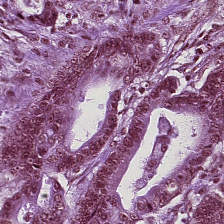
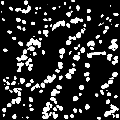
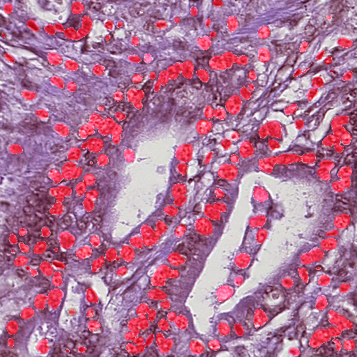
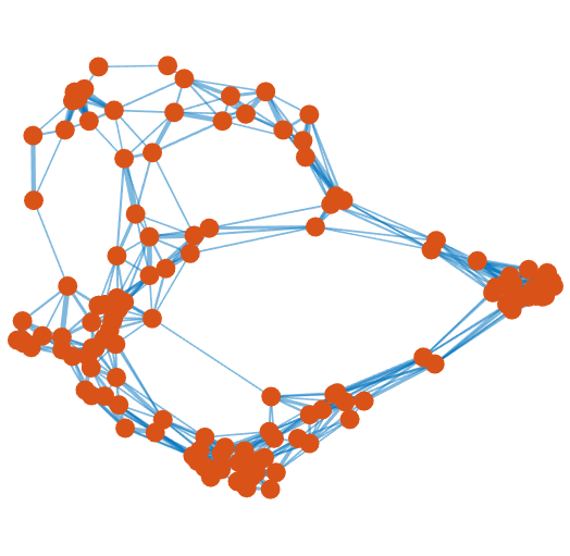
Figure 3: Visualization of the segmented cells and the generated graphs from an arbitrary patch sample of GIST-PDL1. The four subgraphs from left to right are the raw patch image, the segmented cells masks, the patch image with overlaid segmentation masks, and the generated graph.

4 Experiments

4.1 Implementation and Setups

Dataset.

We evaluate the proposed fusion scheme on three real-world H&E stained histology benchmarks, termed as CRC-MSI, STAD-MSI, and GIST-PDL1. The first two datasets targets binary microsatellite instability (MSI) status classification (Kather et al., 2019a), where we follow the original train and test split. We also evaluate the performance of the model on a binary Programmed Death-Ligand 1 (PD-L1) status binary classification dataset, which was curated from $129$ well-annotated WSIs of gastric cancer patients. We supplement further details for data collection and descriptions in Table 1 and Appendix A.

Table 1: Summary of the three datasets.

	Dataset	GIST-PDL1	CRC-MSI	STAD-MSI
IMAGE	# Patients	$129$	$315$	$360$
	# Training Images	$7,676$	$93,408$	$100,570$
	Training Positive Rate	$41.10\%$	$50.0\%$	$50.0\%$
	# Test Images	$2,471$	$99,904$	$118,008$
	Test Positive Rate	$47.71\%$	$29.4\%$	$23.6\%$
	Magnification	$20\times$	$20\times$	$20\times$
	Original Patch Size	$512\times 512$	$224\times 224$	$224\times 224$
GRAPH	Min # Nodes	$50$	$1$	$1$
	Max # Nodes	$621$	$103$	$120$
	Median # Nodes	$199$	$40$	$51$
	Avg # Nodes	$206$	$40$	$50$
	Avg # Edges	$3,402$	$163$	$246$

Model Configurations.

We evaluate the performance gain of our proposed fusion scheme with a comprehensive comparison against three CNN backbones of different scales: MobileNetV3 (Howard et al., 2019), DenseNet (Huang et al., 2017), and ResNet (He et al., 2016). We stack two graph convolution layers for graph representation learning. Two candidates of graph convolution GCN (Kipf and Welling, 2017) and GIN (Xu et al., 2018) are taken into account, following a $2$-layer TopK (Cǎtǎlina et al., 2018) graph pooling scheme. The graph convolution plays the critical role in extracting the geometric feature of the patch. For the fusion layer, both a $1$-layer MLP and Transformer are validated. We name the models in Table 2 with the adopted model architectures and modules. For instance, ResNet-GCN-MLP indicates a ResNet for image embedding, GCN plus TopK for graph representation learning, and MLP MLPBlock for features fusion. We fix the number of layers for each block. For example, we take $121$ convolution layers for DenseNet in all five related models. Details of the model configurations and training hyper-parameters are elaborated in Appendix D.

Table 2: Average test ACC and AUC comparisons on three benchmarks over $7$ repetitions.

		GIST-PDL1			CRC-MSI			STAD-MSI
Model		ACC	AUC	AUCpatient	ACC	AUC	AUCpatient	ACC	AUC	AUCpatient
	GCN	$68.5$$\pm 1.71$	$73.3$$\pm 1.33$	$58.2$$\pm 2.54$	$66.8$$\pm 2.12$	$56.5$$\pm 1.48$	$51.1$$\pm 6.52$	$69.3$$\pm 6.75$	$55.9$$\pm 1.31$	$62.9$$\pm 1.91$
	GIN	$71.9$$\pm 1.37$	$77.2$$\pm 0.81$	$62.9$$\pm 1.43$	$66.6$$\pm 1.79$	$57.0$$\pm 0.91$	$44.6$$\pm 3.39$	$71.3$$\pm 3.52$	$60.3$$\pm 1.22$	$66.8$$\pm 4.09$
MobileNetV3	NA	$73.6$$\pm 2.14$	$86.8$$\pm 1.24$	$83.9$$\pm 4.08$	$73.0$$\pm 0.75$	$66.3$$\pm 0.55$	$64.7$$\pm 3.09$	$75.3$$\pm 1.26$	$66.9$$\pm 2.11$	$72.8$$\pm 1.15$
	GCN-MLP	$77.2$$\pm 0.68$	$88.7$$\pm 0.51$	$92.0$$\pm 0.36$	$72.7$$\pm 0.34$	$73.5$$\pm 0.60$	$77.5$$\pm 2.82$	$76.1$$\pm 0.42$	$71.9$$\pm 0.86$	$73.1$$\pm 0.99$
	GIN-MLP	$74.9$$\pm 1.23$	$89.4$$\pm 0.36$	$94.2$$\pm 2.28$	$73.4$$\pm 0.20$	$69.1$$\pm 3.80$	$78.1$$\pm 3.98$	$75.8$$\pm 0.37$	$69.8$$\pm 1.01$	$73.2$$\pm 0.79$
	GCN-Trans	$77.9$$\pm 1.17$	$90.5$$\pm 0.86$	$96.7$$\pm 1.02$	$73.2$$\pm 0.44$	$71.0$$\pm 0.76$	$77.8$$\pm 3.70$	$76.3$$\pm 0.41$	$73.6$$\pm 0.70$	$74.3$$\pm 0.64$
	GIN-Trans	$76.2$$\pm 1.37$	$90.9$$\pm 0.86$	$94.4$$\pm 1.80$	$73.5$$\pm 0.37$	$70.5$$\pm 1.33$	$79.5$$\pm 2.40$	$76.3$$\pm 0.68$	$73.4$$\pm 1.44$	$74.4$$\pm 1.51$
DenseNet	NA	$71.2$$\pm 1.42$	$82.5$$\pm 3.25$	$89.0$$\pm 4.29$	$74.2$$\pm 0.28$	$70.0$$\pm 0.91$	$66.7$$\pm 4.83$	$74.9$$\pm 1.68$	$65.5$$\pm 1.08$	$74.9$$\pm 0.03$
	GCN-MLP	$76.5$$\pm 0.90$	$88.9$$\pm 0.78$	$95.9$$\pm 3.50$	$75.2$$\pm 0.29$	$70.0$$\pm 1.08$	$68.2$$\pm 2.22$	$76.6$$\pm 0.40$	$74.5$$\pm 0.99$	$75.9$$\pm 1.24$
	GIN-MLP	$76.7$$\pm 0.71$	$88.0$$\pm 0.67$	$94.6$$\pm 1.19$	$74.6$$\pm 0.24$	$70.1$$\pm 0.88$	$71.6$$\pm 1.32$	$77.0$$\pm 0.33$	$74.8$$\pm 1.13$	$75.4$$\pm 0.74$
	GCN-Trans	$79.6$$\pm 0.76$	$89.8$$\pm 1.08$	$97.5$$\pm 1.57$	$74.9$$\pm 0.36$	$74.0$$\pm 0.59$	$83.2$$\pm 2.05$	$76.7$$\pm 0.79$	$73.6$$\pm 0.71$	$76.3$$\pm 1.06$
	GIN-Trans	$75.8$$\pm 1.51$	$87.7$$\pm 1.09$	$96.0$$\pm 2.00$	$74.8$$\pm 0.54$	$74.6$$\pm 0.63$	$75.7$$\pm 3.17$	$76.8$$\pm 0.58$	$74.4$$\pm 1.00$	$75.8$$\pm 0.95$
ResNet	NA	$70.7$$\pm 2.09$	$82.1$$\pm 1.53$	$86.3$$\pm 1.65$	$73.5$$\pm 0.40$	$65.3$$\pm 3.95$	$61.7$$\pm 4.97$	$73.8$$\pm 1.51$	$72.6$$\pm 0.95$	$74.1$$\pm 0.82$
	GCN-MLP	$81.9$$\pm 3.46$	$92.6$$\pm 1.52$	$94.1$$\pm 3.43$	$74.2$$\pm 0.43$	$75.2$$\pm 0.85$	$83.2$$\pm 1.26$	$76.0$$\pm 0.63$	$73.1$$\pm 0.79$	$74.8$$\pm 0.75$
	GIN-MLP	$76.3$$\pm 2.02$	$87.6$$\pm 2.48$	$91.3$$\pm 2.57$	$74.5$$\pm 0.70$	$69.9$$\pm 2.19$	$83.0$$\pm 1.67$	$76.2$$\pm 0.42$	$74.7$$\pm 0.89$	$75.6$$\pm 2.17$
	GCN-Trans	$76.0$$\pm 1.78$	$86.4$$\pm 2.68$	$93.7$$\pm 3.64$	$74.8$$\pm 0.32$	$73.6$$\pm 1.28$	$84.7$$\pm 2.11$	$76.1$$\pm 0.80$	$72.7$$\pm 0.45$	$75.6$$\pm 1.23$
	GIN-Trans	$76.8$$\pm 1.08$	$92.1$$\pm 0.57$	$95.5$$\pm 0.94$	$74.6$$\pm 0.47$	$73.4$$\pm 0.77$	$83.8$$\pm 1.65$	$76.2$$\pm 0.41$	$74.6$$\pm 0.24$	$75.8$$\pm 1.71$

4.2 Results and Analysis

Image-level performance is evaluated with two metrics, namely test accuracy (ACC) and area-under-curve (AUC). Similarly, we evaluate patient-level prediction with AUC (denoted as AUCpatient). As shown in Table 2, the fused learning schemes achieve more than $5\%$ performance gain over plain CNNs. The improvement is more significant at the patient level at up to $23\%$. The additional performance boost suggests that our design of the integrated scheme has better potential to overcome the disturbance of heterogeneous patches for patient-level overall diagnosis. The main takeaways include: 1) An individual GNN fails to achieve satisfactory performance. But as a parallel layer, GNNs can enhance the learning capability of CNN by a learnable fusion layer. 2) MLP, though simple, serves as a good fusion layer. 3) Generally speaking, the Transformer integrator outperforms the simple MLP scheme. However, one can not tell whether MLP or Transformer is a universally better fusion solution. 4) All the integrated models outperform the plain CNNs or GNNs. 5) For the choice of a GNN module, GCN and GIN do not present a significant advantage one over the other. More empirical investigations are supplemented in Appendix E, including training cost, performance improvement rate, as well as the performance ranking.

We also investigate the overall ranking of each model fusion configuration in Table 3. We report the averaged ranking for every CNN architecture over three datasets, where in each dataset ranks are calculated by sorting the reported scores. Generally, the Transformer integrator outperforms the simple MLP scheme. For the choice of GNNs, GCN and GIN do not present a significant advantage one over another. Nevertheless, all the integrated models outperform designs with plain CNNs.

Table 3: Performance ranking reports the average rank across three datasets. For simplicity, MV3,Dense and Res denote MobileNetV3, DenseNet-121 and ResNet-18 respectively. The ‘Avg’ columns report the averaged ranking over three CNN architectures.

	ACC				AUC				AUCpatient
	MV3	Dense	Res	Avg	MV3	Dense	Res	Avg	MV3	Dense	Res	Avg	Overall
CNN	4.7	5.0	5.0	4.9	5.0	5.0	5.0	5.0	5.0	5.0	5.0	5.0	5.0
GCN-MLP	3.3	2.7	3.0	3.0	2.3	2.7	1.7	2.2	4.0	3.0	3.0	3.3	2.9
GCN-Trans	3.3	2.3	2.3	2.7	4.0	2.3	2.7	3.0	2.7	3.7	3.3	3.2	3.0
GIN-MLP	1.7	2.0	2.7	2.1	1.7	2.3	3.3	2.4	2.0	1.0	2.3	1.8	2.1
GIN-Trans	2.0	3.0	2.0	2.3	2.0	2.7	2.3	2.3	1.3	2.3	1.3	1.7	2.1

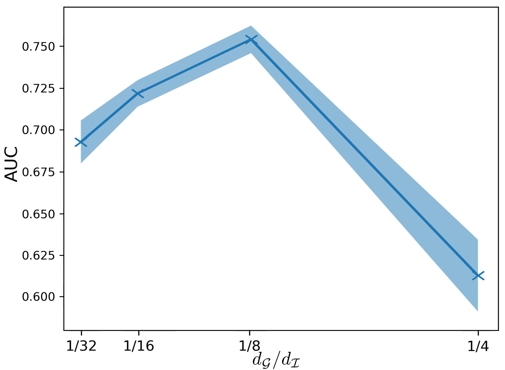
Figure 4: The image-level test AUC of CRC-MSI is sensitive to different choices of $d_{\mathcal{G}}/d_{\mathcal{I}}$.

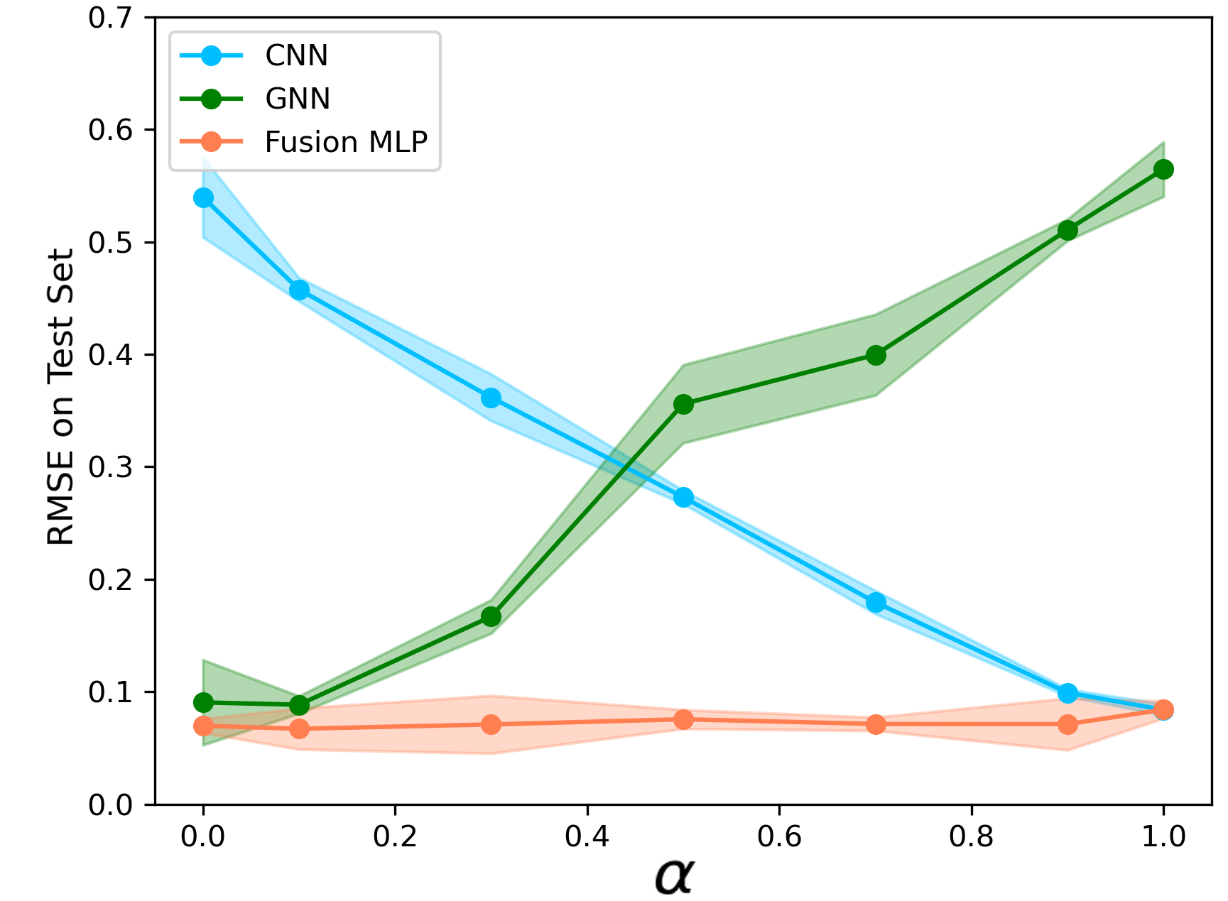
Figure 5: Test RMSE in synthetic task. The fusion model consistently outperforms CNN/GNN.

4.3 Ablation Study

In MLP fusion scheme where feature alignment is not necessary, we found the performance is sensitive to the the dimension of ${\bm{H}}_{\mathcal{I}}$, ${\bm{H}}_{\mathcal{G}}$. In Figure 5, we present ablations on $d_{\mathcal{G}}/d_{\mathcal{I}}$ with CRC-MSI, where we use GIN and ResNet18 as the backbones and consequently $d_{\mathcal{I}}$ is fixed to 512 (see supplementary for details). Thus, $d_{\mathcal{G}}/d_{\mathcal{I}}$ needs to be carefully tuned to achieve satisfactory performance in the MLP fusion scheme. On the contrast, with the feature alignment, Transformer fusion layers are easier to train.

5 How Fusion Scheme Works?

In this section, a synthetic task is constructed to explore how the fusion scheme works. Specifically, each image ${\bm{X}}_{\mathcal{I}}$ in MNIST and its associated superpixel graph ${\bm{X}}_{\mathcal{G}}$ in MNISTSuperpixel (Monti et al., 2017) form a paired data $({\bm{X}}_{\mathcal{I}},{\bm{X}}_{\mathcal{G}})$, and we retain their original training and test data partition. Instead of using the classification label, we synthesize the regression objects which can manually adjust the proportion of image-level and geometric representations:

$$y=\alpha\cdot f_{\texttt{CNN}}({\bm{X}}_{\mathcal{I}})+(1-\alpha)\cdot f_{\texttt{GNN}}({\bm{X}}_{\mathcal{G}}),$$ (12)

where $f_{\texttt{CNN}}$ and $f_{\texttt{GNN}}$ denote the averaged prediction from 30 randomly initialized ResNet18 and GIN2 (with seed=$0,1,\cdots,29$) respectively (details are elaborated in supplementary). The $f_{\texttt{CNN}}(\mathbf{x}_{\mathcal{I}})$ and $f_{\texttt{GNN}}(\mathbf{x}_{\mathcal{G}})$ are fixed once they are generated. We suppose that $f_{\texttt{CNN}}$ produces objects easier for LeNet5 to learn, and $f_{\texttt{GNN}}$ easier for GCN2. The coefficient $\alpha\in[0,1]$ balances the learning difficulty of CNN or GNN, and also the proportion of image-level and geometric-level features used in model prediction. Specifically, the large value of $\alpha$ represents higher proportion of image-level features, thus easier for CNN to learn. The objective $y$s are normalized for both training and testing. Comparisons of GNN, CNN and the fusion framework with MLP on $\alpha\in\{0.0,0.1,0.3,0.5,0.7,0.9,1.0\}$ are illustrated in Figure 5. The test RMSE of LeNet5 monotonically decrease with a larger $\alpha$; while RMSE of GCN increases. It yields that GCN fails achieve parallel results as LeNet5 when the task is more CNN-friendly (e.g.,  $\alpha\geq 0.5$ in our setting). Similarly, when the geometric information is dominant (e.g.,  $\alpha\leq 0.5$), LeNet5 fails to capture comprehensive representations. Our fusion scheme, performs universally better than either LeNet5 or GCN at any ratio between the geometric and morphological representations. The improvement reaches its peak in the range $\alpha\in[0.3,0.7]$, which coincides with the hypothesized settings in various medical image analysis tasks. Furthermore, when the task tends to be more CNN/GNN-friendly, the fusion model, though slight, keeps outperforming CNN/GNN. It confirms that the features extracted by CNN and GNN are complementary from two views i.e., textural and geometric, thus should be considered jointly.

6 Related Work

Deep Learning for Large-scale Medical Imaging and Biomarker Prediction.

Deep learning has become the mainstream choice to assess disease in gigapixel WSIs (Thomas et al., 2013; LeCun et al., 2015; Madabhushi and Lee, 2016; Shen et al., 2017). Various applications are developed upon the success of deep learning and computer vision for histology diagnostic tasks, such as breast cancer segmentation Cruz-Roa et al. (2014), prostate cancer detection (Litjens et al., 2016), and sentinel lymph nodes detection (Litjens et al., 2018). Biomarkers (Duffy, 2013; Villalobos and Wistuba, 2017) are the clinical indicators for tumor behavior that distinguish patients who will benefit from certain molecular therapies. Previous works show that deep learning can predict specific genetic mutations in non–small cell lung cancer from hematoxylin and eosin (H&E) stained slides (Schaumberg et al., 2018; Coudray et al., 2018; Kim et al., 2020; Sha et al., 2019; Echle et al., 2021b). Much progress have been made in microsatellite instability (MSI) or mismatch repair deficiency (dMMR) in colorectal cancer (CRC) (Kather et al., 2019b; Schmauch et al., 2020; Ke et al., 2020; Cao et al., 2020; Echle et al., 2020; Bilal et al., 2021; Yamashita et al., 2021) Test AUC is risen up to 0.99, which thus even inspired wide commercial interests (Echle et al., 2021a).

Graph Neural Networks for Medical Imaging.

CNNs have gained in successfully aiding the diagnostic process for histology arises from their capability to discover hierarchical feature representations without domain expertise (Shen et al., 2017). However, the spatial relations, as well as the formulation of structured information, are absent, where this prior is crucial to real clinical diagnosis (Barua et al., 2018; Feichtenbeiner et al., 2014; Galon et al., 2006). GNNs provide an alternative to CNN in its capability of describing relationships and structures (Bronstein et al., 2017; Wu et al., 2020; Zhang et al., 2020; Bronstein et al., 2021). As a powerful approach to model functional and anatomical structures, the graph-based deep learning approaches have exhibited substantive success for various tasks in the histology domain (Lu et al., 2021; Wang et al., 2021; Noble et al., 2022). By capturing the geometrical and topological representations, the mutual interaction between cells can be learned by a neural network.

7 Discussion

Limitations.

The fusion scheme takes paired image and graph as input. The graph should be extracted prior to the training stage. However, the construction of the graph is task-specific, with the reliance on domain knowledge. Consequently, detailed analysis should be conducted to discover whether the geometric information contributes to the prediction tasks.

Broader Impact.

In the application to clinical practice, fusing the graph representations with image representations enables domain experts to incorporate their prior knowledge to modeling. For example, in histology analysis, the construction of cell graphs and the determination of the critical distance reflect how doctors expect cells to interact with each other. However, incorporation of the improper prior knowledge to the graph formulations may bring negative effect to the training process, hence should be carefully assessed. It also points out an interesting future direction towards the automatically generated graph from image with limited human involvement.

8 Conclusion

This work proposes a fusion framework for learning the topology-embedded images by CNN and GNN. Furthermore, we present a use case of the fusion model to biomarker prediction tasks from histology slides, where the geometric information are proven to be important. Specifically, we integrate GNN to add local geometric representations for cell-graph patches on top of CNNs which extracts a global image feature representation. The CNNs and GNNs are trained in parallel and their output features are integrated in a learnable fusion layer. This is important as the fusion scheme addresses the expression of the tumor microenvironment by supplementing topology inside local patches in network training. We validate the framework using different combinations of CNN, GNN and fusion modules on real H&E stained histology datasets, which surpasses the plain CNN or GNN methods to a significant margin. The experiments yield that the geometric feature and image-level feature are complementary. Finally, the constructed image-graph bimodal datasets can serve as benchmark for future study.

Appendix A Dataset

This section reveals details for three real-world benchmark datasets. We start by reviewing the two public datasets, i.e., CRC-MSI of colorectal cancer patients and STAD-MSI of gastric adenocarcinoma cancer patients for microstatellite status prediction, as well as a privately curated gastric cancer dataset (GIST-PDL1) for PD-L1 status classification. In Table 1, we brief three datasets with the numerical statistics.

A.1 CRC-MSI and STAD-MSI

The two public datasets focus on the prediction of distinguishing the microsatellite instability (MSI) from microsatellite stability (MSS) in H&E stained histology. Notably, MSI is a crucial clinical indicator for oncology workflow in the determination of whether a cancer patient responds well to immunotherapy. It is not until very recently that researches have shown the promising performance of deep learning methods in MSI prediction. With the lack of an abundant number of annotated histology, MSI prediction is still very challenging. Thus, it is required to incorporate prior knowledge such as geometric representation for MSI prediction.

In the experiment, the two datasets classify images patches to either MSS (microsatellite stable) or MSIMUT (microsatellite instable or highly mutated). We treat MSIMUT as the positive label and MSS as the negative label in computing the AUC. The original whole-slide images (WSIs) are derived from diagnostic slides with formalin-fixed paraffin-embedded (FFPE) processing. In particular, CRC-MSI contains H&E stained histology slides of $315$ colorectal cancer patients, and STAD-MSI includes H&E slides of $360$ gastric cancer patients. For both datasets, a WSI with respect to a patient is tessellated into non-overlapped patches/images with a resolution of $224\times 224$ pixels at the magnification of 20$\times$. The patches from $70\%$ patients are used for training and the remaining patches from $30\%$ patients are left for validation. Note that each patient is associated with only one WSI. Yet, the number of generated image patches from one WSI varies from each other. Consequently, the ratios of training and test image samples depicted in Table 1 for CRC-MSI and STAD-MSI are not $70\%:30\%$ as its patient-level ratio.

A.2 GIST-PDL1

The privately collected GIST-PDL1 predicts programmed death-ligand 1 (PD-L1) status from gastric cancer histology slides. PD-L1 is a type of immune-checkpoint protein from tumor cells that disturbs the body’s immune system through binding programmed death 1 (PD-1) on T cells. The PD-L1 expression is one of the only established biomarkers that determine the efficacy of immunotherapy in gastric and esophageal cancer in advanced stages (Smyth et al., 2021).

This dataset collects $129$ well-annotated H&E stained histology slides of gastric cancer patients between the year 2020 and the year 2021 from [anonymous] hospital, with ethical approval. Each whole-slide image (WSI) corresponds to one patient, where the patient is labeled as either positive (CPS$\geq 5$) or negative (CPS$<5$) determined by its PD-L1 combined positive score (CPS) tested from the immunohistochemistry (IHC) test. The patch-level annotation inherits the associated patient/WSI-level label. The resolution of a WSI is around $10,000\times 10,000$ pixels, which is split into non-overlapping images (patches) of $512\times 512$ pixels at the magnification $20\times$, and afterward resized to $224\times 224$ to get aligned with the two public datasets. Background patches are excluded for downstream analysis with OTSU algorithm, where the remaining patches are subsequently stain normalized to reduce the data heterogeneity. Each patch comprises approximately $200$ cells i.e., nodes. Different from CRC-MSI and STAD-MSI, we conduct down-sampling on the number of image patches from each WSI to balance the ration between positive and negative samples. Consequently, we achieve a balanced image-level sample ratio that is close to $50\%:50\%$.

A.3 Data Availability

The two public datasets for MSI classification with their annotations freely available at

$$\text{{https://doi.org/10.5281/zenodo.2530834}}.$$

The private dataset along with the established graph data for three benchmarks will be released after acceptance.

Appendix B Nuclei Segmentation

In the node construction process, we employ CA^2.5-Net (Huang et al., 2021) as the backbone for nuclei segmentation, due to its outstanding performance in challenging clustered edges segmentation tasks, which frequently occurs in histology analysis. We use the implementation at https://github.com/JH-415/CA2.5-net. Specifically, CA^2.5-Net formulates nuclei segmentation task in a multi-task learning paradigm that uses edge and cluster edge segmentation to provide extra supervision signals. To be more concretely, the decoder in CA^2.5-Net comprises three output branches that learn the nuclei semantic segmentation, normal-edge segmentation (i.e., non-clustered edges), and clustered-edge segmentation respectively. A proportion of the convolutional layers and upsampling layers in the CA^2.5-Net is shared to learn common morphological features. We follow the original settings (Huang et al., 2021) by using the IoU loss for the segmentation path of the nuclei semantic ($\mathcal{L}_{sem}$) and the smooth truncated loss for segmentation paths of normal-edges ($\mathcal{L}_{nor}$) and clustered-edges ($\mathcal{L}_{clu}$). Formally, the overall loss thus takes a weighted average over the three terms of segmentation losses, i.e.,

$$\mathcal{L}=\alpha\cdot\mathcal{L}_{sem}+\beta\cdot\mathcal{L}_{nor}+\gamma\cdot\mathcal{L}_{clu}.$$ (13)

In particular, we applies the balancing coefficients $\alpha=0.7$, $\beta=0.2$, and $\gamma=0.1$. We trained CA^2.5-Net with Adam optimizer for $50$ epochs, with an initial learning rate of $1\times 10^{-4}$ that decayed by $0.95$ for every other epochs. At the inference stage of nuclei locations, we adopt the nuclei segmentation path to derive the prediction result.

Three well-experienced pathologists annotated a number of $132$ image patches from GIST-PDL1 for training the CA^2.5-Net, where we use $100$ images for training and the remaining $32$ for validation. To increase the data variations, we adopt offline augmentation (i.e., images are augmented prior to the training stage) by randomly flipping and rotating for 90 degrees. Eventually, we come to a total number of $400$ training samples. For illustration purposes, we pick one annotated sample and show it in Figure 6. The pixel-level instance annotations were conducted with ‘labelme’ (https://github.com/wkentaro/labelme), where the semantic masks can be generated directly from the instance segmentation (Huang et al., 2021).

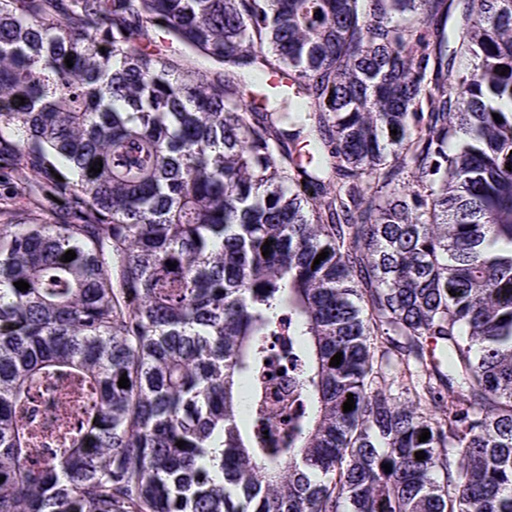
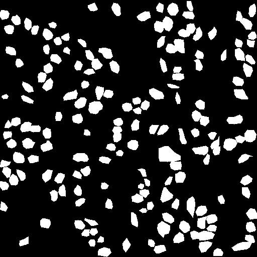
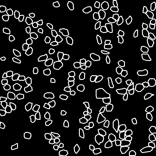
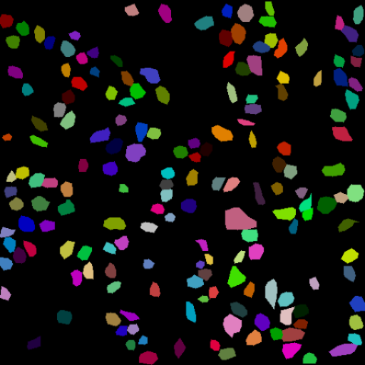
Figure 6: An illustrative example of annotated histology patch from GIST-PDL1 for training the nuclei segmentation network. The four subgraphs from left to right are the raw patch image, the generated semantic nuclei masks, the generated semantic nuclei edge, and the annotated instance nuclei mask (ground truth).

Table 4: The pre-defined node attributes computed for each nuclei area.

GLCM	GLDM	GLRLM
autocorrelation	dependence entropy	gray-level non-uniformity
cluster prominence	dependence non-uniformity	gray-level non-uniformity normalized
cluster shade	dependence non-uniformity normalized	gray-level variance
cluster tendency	dependence variance	high gray-level run emphasis
contrast	gray-level non-uniformity	long-run emphasis
correlation	gray-level variance	long-run high gray-level emphasis
difference average	high gray-level emphasis	long-run low gray-level emphasis
difference entropy	large-dependence emphasis	low gray-level run emphasis
difference variance	large-dependence high gray-level emphasis	run entropy
inverse difference	large-dependence low gray-level emphasis	run length non-uniformity
inverse difference moment	low gray-level emphasis	run length non-uniformity normalized
inverse difference moment normalized	small-dependence emphasis	run percentage
inverse difference normalized	small-dependence high gray-level emphasis	run variance
informational measure of correlation 1	small-dependence low gray-level emphasis	short-run emphasis
informational measure of correlation 2		short-run high gray-level emphasis
Inverse variance		short-run low gray-level emphasis
joint average	FIRST-ORDER
joint energy	10 percentile
joint entropy	90 percentile	GLSZM
maximal correlation coefficient	energy	gray-level non-uniformity
maximum probability	entropy	gray-level non-uniformity normalized
sum average	inter quartile range	gray-level variance
sum entropy	kurtosis	high gray-level zone emphasis
sum squares	maximum	large area emphasis
	mean absolute deviation	large area high gray-level emphasis
LOCATION	mean	large area low gray-level emphasis
center of mass-x	median	low gray-level zone emphasis
center of mass-y	minimum	size zone non-uniformity
	range	size zone non-uniformity normalized
NGTDM	robust mean absolute deviation	small area emphasis
busyness	root mean squared	small area high gray-level emphasis
coarseness	skewness	small area low gray-level emphasis
complexity	total energy	zone Entropy
contrast	uniformity	zone Percentage
strength	variance	zone variance

Appendix C Node Feature Extraction

This section details the essential pre-processing of the raw histology input (i.e., images) to extract morphological features as node attributes in the construction of cell graphs. The same procedure applies to all three datasets. The segmentation results of CA^2.5-Net on slide patches generate nodes of graphs. For an arbitrary patch, a graph is generated where nodes represent cells and the weighted edges reveal the Euclidean distance between nodes.

Next, we select $94$ features from pathomics, i.e., a pre-defined feature library for medical image analysis (Lambin et al., 2017) that describe the location, first-order statistics, and the gray-level textural features of each segmented cell. To be specific, the five dimensions of the spatial distribution include gray-level co-occurrence (GLCM), gray-level distance-zone (GLDM), gray-level run-length (GLRLM), gray-level size-zone (GLSZM), and neighborhood gray tone difference (NGTDM). In total, there are $2$ coordinates of the cell location, $18$ values of the first-order statistics, $24$ GLCM, $14$ GLDM, $16$ GLRLM, $16$ GLSZM, and $5$ NGTDM. We give the name of all $94$ features in Table 4 for a better understanding. For a detailed calculation of each attribute, we refer interested readers to Lambin et al. (2017).

Appendix D Implementation Details

The code is available at:

https://anonymous.4open.science/r/gnncnnfusion2243/

We will replace this anonymous link with a non-anonymous GitHub link after the acceptance. All the experiments are implemented in Python 3.8.12 environment on one NVIDIA ^® Tesla A100 GPU with 6,912 CUDA cores and 80GB HBM2 mounted on an HPC cluster. We implement GNNs on PyTorch-Geometric (version 2.0.3) and CNNs on PyTorch (version 1.10.2). All CNNs have used ImageNet pre-trained weights provided by TIMM library.

D.1 Training Settings

All the model architectures follow the training scheme with the hyper-parameters listed in Table 5. We employ the standard cross-entropy as the loss function. The training stage continues until stopping improvements on the validation set after $8$ consecutive epochs.

Table 5: Hyper-parameters for training the models.

Hyper-parameters	Value
Initial learning rate	$5\times 10^{-4}$
Minimum learning rate	$5\times 10^{-6}$
Scheduler	Cosine Annealing (T_max=$10$)
Optimizer	AdamW
Weight Decay	$1\times 10^{-5}$
Num_workers	$12$
Batch size	$256$
Maximum epoch number	$100$

D.2 Model Configuration

Table 6 describes the configuration of MLP fusion layer, Transformer fusion layer, GCN and GIN used in this research. The model architectures for all three datasets have adopted the same configuration. The output for GCN and GIN are set to the same size 16, without fine-tuning for each dataset, and for CNNs we use the default output size. In Transformer fusion layer, we use the Minimization Alignment strategy to reduce the computational cost.

Table 6: Default configurations.

MLP	# MLPBlock	$1$
	Feature embedding size	$128$
	Activation	Leaky ReLU
	Dropout rate	$0.1$
Transformer	# TransBlock	$1$
	Feature embedding size	$192$
	Activation	ReGLU
	# Attention heads	$4$
	Dropout rate in TransBlock	$0.1$
	Alignment strategy	Minimization Alignment
GCN and GIN	# layers	$2$
	Feature embedding size	$128$
	Activation	GeLU

D.3 Data Augmentations

To improve the model generalization, we perform online data augmentation for both graphs and images in the training stage. The graph data is augmented with RandomTranslate where the translate is set to 5. Images are first resized to $224\times 224$ pixels, and then augmented by Random Horizontal Flip, Random Vertical Flip, and Random Stain Normalization and Augmentation. Random Stain Normalization and Augmentation is designed to spec targets to alleviate the stain variations specifically for histology, where stain normalization template is randomly generated per iteration.

D.4 Comparison on the Number of Trainable Parameters

Table 7 reports the number of trainable parameters of all the models we evaluated in Table 2. The values are given with the image input size of $3\times 224\times 224$ and the node feature dimension of $94$. The scale of the trained model is jointly determined by the choice of modules in CNN, GNN, and fusion layers, where we highlighted different options by color. The choice of colors aligns with the associated modules visualized in Figure 2. For instance, green colors include three selections of CNN modules, including MobileNetV3, DenseNet, and ResNet. ‘N/A’ indicates an absence of such layers in the framework. The numbers are reported in millions ($1\times 10^{6}$). For instance, $13.1277$ at the bottom-right of the table means that it involves $13.1277$ millions of learnable parameters when training an integrated model with the ResNet18-GIN2-Trans architecture.

Table 7: Comparison on the number of trainable parameters (in millions).

		CNN
GNN	Fusion	N/A	MobileNetV3	DenseNet	ResNet
N/A	N/A	-	$1.7865$	$7.2225$	$11.3110$
	MLP	0.0665	$1.8506$	$7.2866$	$11.3751$
GCN	Transformer	-	$8.4943$	$13.9303$	$13.1231$
	MLP	$0.0712$	$1.8552$	$7.2912$	$11.3797$
GIN	Transformer	-	$8.4989$	$13.9349$	$13.1277$

Appendix E Further Performance Analysis

Table 8: Test Acc and AUC improvements of the fusion model to pure CNN on three benchmarks.

		GIST-PDL1			CRC-MSI			STAD-MSI
Model		$\Delta$ACC	$\Delta$AUC	$\Delta$AUCpatient	$\Delta$ACC	$\Delta$AUC	$\Delta$AUCpatient	$\Delta$ACC	$\Delta$AUC	$\Delta$AUCpatient
MobileNetV3	GCN-MLP	$3.56$	$1.96$	$8.06$	$-0.25$	$7.17$	$12.87$	$0.78$	$4.98$	$0.35$
	GIN-MLP	$1.33$	$2.59$	$10.32$	$0.43$	$2.79$	$13.47$	$0.53$	$2.90$	$0.46$
	GCN-Trans	$4.27$	$3.69$	$12.82$	$0.19$	$4.75$	$13.16$	$1.01$	$6.73$	$1.53$
	GIN-Trans	$2.56$	$4.16$	$10.51$	$0.51$	$4.24$	$14.89$	$0.95$	$6.47$	$1.65$
DenseNet	GCN-MLP	$5.35$	$6.35$	$6.89$	$1.04$	$0.07$	$1.60$	$1.66$	$8.96$	$1.04$
	GIN-MLP	$5.58$	$5.51$	$5.61$	$0.46$	$0.16$	$4.95$	$2.07$	$9.25$	$0.58$
	GCN-Trans	$8.45$	$7.29$	$8.47$	$0.81$	$4.01$	$16.60$	$1.77$	$8.04$	$1.44$
	GIN-Trans	$4.64$	$5.20$	$6.99$	$0.65$	$4.64$	$9.08$	$1.90$	$8.82$	$0.98$
ResNet	GCN-MLP	$11.25$	$10.50$	$7.81$	$0.62$	$9.84$	$21.50$	$2.26$	$0.50$	$0.66$
	GIN-MLP	$5.61$	$5.51$	$5.04$	$0.99$	$4.54$	$21.33$	$2.43$	$2.13$	$1.49$
	GCN-Trans	$5.39$	$4.31$	$7.39$	$1.26$	$8.33$	$23.04$	$2.35$	$0.10$	$1.43$
	GIN-Trans	$6.16$	$9.99$	$9.27$	$1.08$	$8.12$	$22.13$	$2.42$	$1.99$	$1.71$

Table 8 below reveals the absolute percentage improvement of each metrics in the main prediction tasks. The comparisons are made on basis of CNNs methods. To be specific, an absolute improvement score is calculated by

$$\Delta\text{ Score}=S_{\text{fused}}-S_{\text{CNN}},$$

where $S_{\text{CNN}}$ denotes the performance score (i.e.,  ACC, AUC or AUCpatient) achieved by plain CNNs (e.g., MobileNetV3, DenseNet or ResNet), and $S_{\text{fused}}$ is the associated score by integrated models, which are listed in the first column at the very left. For instance, the $3.56$ at the top-left of the table means that the test accuracy of MobileNetV3-GCN-MLP is improved by $3.56\%$ to MobileNetV3.

Appendix F Visualization of Nuclei Segmentation and Cell Graph

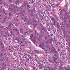
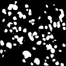
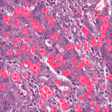
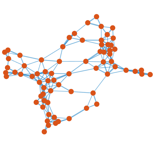
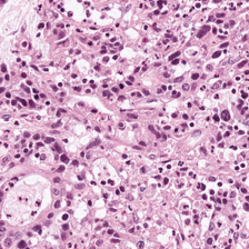
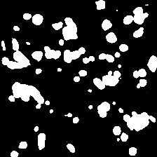
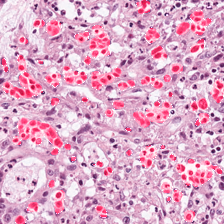
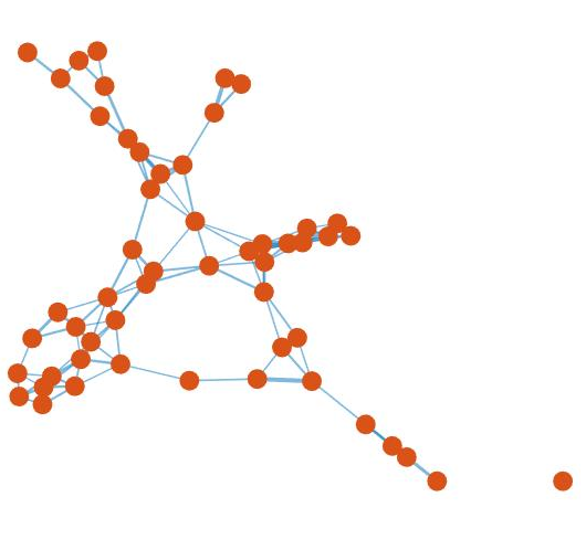
Figure 7: Visualization of the segmented cells and the generated graphs from an arbitrary patch sample of CRC-MSI. The four subgraphs from left to right are the raw patch image, the segmented cells masks, the patch image with overlaid segmentation masks, and the generated graph.

Figure 8: Visualization of the segmented cells and the generated graphs from an arbitrary patch sample of STAD-MSI. The four subgraphs from left to right are the raw patch image, the segmented cells masks, the patch image with overlaid segmentation masks, and the generated graph.

To better understand the learned graphs that are generated from histology images, Figures 3-8 investigate some random patch images from the three datasets and visualize the nuclei segmentation results and the associated graphs. In particular, the four subgraphs from left to right of each figure display the raw patch image, the segmented cells masks, the patch image with overlaid segmentation masks, and the generated graph.

Appendix G Synthetic Task

Data.

The MNIST images are provided by torchvision.datasets.mnist, and the associated superpixel graph is provided by torch_geometric.datasets.mnist_superpixels. Images and graphs are paired based on their sample index.

Regression Label Normalization.

We normalize $f_{\texttt{CNN}}({\bm{X}}_{\mathcal{I}})$ separated for train and test sets by:

$$f_{\texttt{CNN}}({\bm{X}}_{\mathcal{I}})_{\text{normalized}}=\frac{f_{\texttt{CNN}}({\bm{X}}_{\mathcal{I}})_{\text{raw}}-\texttt{Mean}\big{(}f_{\texttt{CNN}}({\bm{X}}_{\mathcal{I}})_{\text{raw}}\big{)}}{\texttt{STD}\big{(}f_{\texttt{CNN}}({\bm{X}}_{\mathcal{I}})_{\text{raw}}\big{)}},$$ (14)

where we use the subscript ‘normalized’ and ‘raw’ to denote the post-processed and pre-processed targets. $f_{\texttt{GNN}}({\bm{X}}_{\mathcal{G}})$ is normalized in the same fashion. The histogram in Figure 9 depicts the label distribution on the training set.

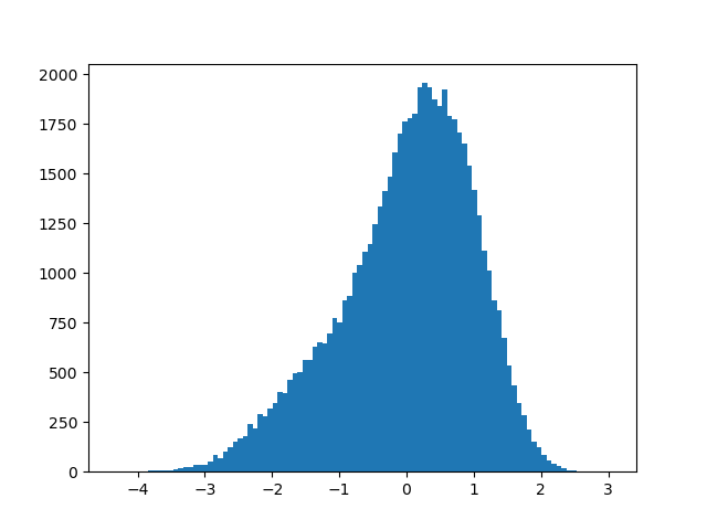
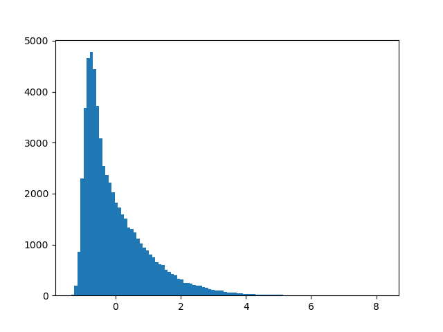
Figure 9: The distribution of normalized $f_{\texttt{CNN}}({\bm{X}}_{\mathcal{I}})$ (left) and $f_{\texttt{GNN}}({\bm{X}}_{\mathcal{G}})$ (right) on the training set.

Label Distributions.

In Figure 10, a significant difference can be observed from the $f_{\texttt{CNN}}({\bm{X}}_{\mathcal{I}})$ and $f_{\texttt{GNN}}({\bm{X}}_{\mathcal{G}})$, which matches our hypothesis that they are easy for different structures to learn.

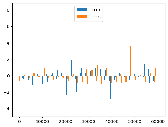
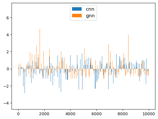
Figure 10: The normalized $f_{\texttt{CNN}}({\bm{X}}_{\mathcal{I}})$ and $f_{\texttt{GNN}}({\bm{X}}_{\mathcal{G}})$ used to construct synthetic label $y$ for training set (left) and test set (right). The $x$-axis is the sample index provided by the original datasets.

Model Configurations.

The configurations of fusion MLP and GIN for synthetic tasks are depicted in Table 9. A clear difference can be observed between the ground truth of $f_{\texttt{CNN}}({\bm{X}}_{\mathcal{I}})$ and $f_{\texttt{GNN}}({\bm{X}}_{\mathcal{G}})$. The LeNet5 follows the default configurations.

Table 9: Hyper-parameter configurations for the synthetic task.

MLP	# MLPBlock	$1$
	Feature embedding size	$10$
	Activation	Leaky ReLU
	Dropout rate	$0.1$
GIN	# layers	$2$
	Feature embedding size	$32$
	Activation	GeLU

Training Scheme.

We select mean square error (MSE) as the loss function, with other hyper-parameters presented in Table 10. We use root mean square error (RMSE) as the evaluation metric. We stop training if the test RSME does not decrease for 10 epochs. For each $\alpha$, we perform 5 random runs and report the mean and standard deviation.

Table 10: Hyper-parameters for training the model in the synthetic task.

Hyper-parameters	Value
Scheduler	Constant
Optimizer	AdamW
Learning rate	$1\times 10^{-4}$
Weight Decay	$1\times 10^{-5}$
Num_workers	$10$
Batch size	$256$
Maximum epoch number	$10,000$

Analysis.

The performance improvement of fusion model to CNN (LeNet5) and GNN (GIN2) is shown in Figure 11.

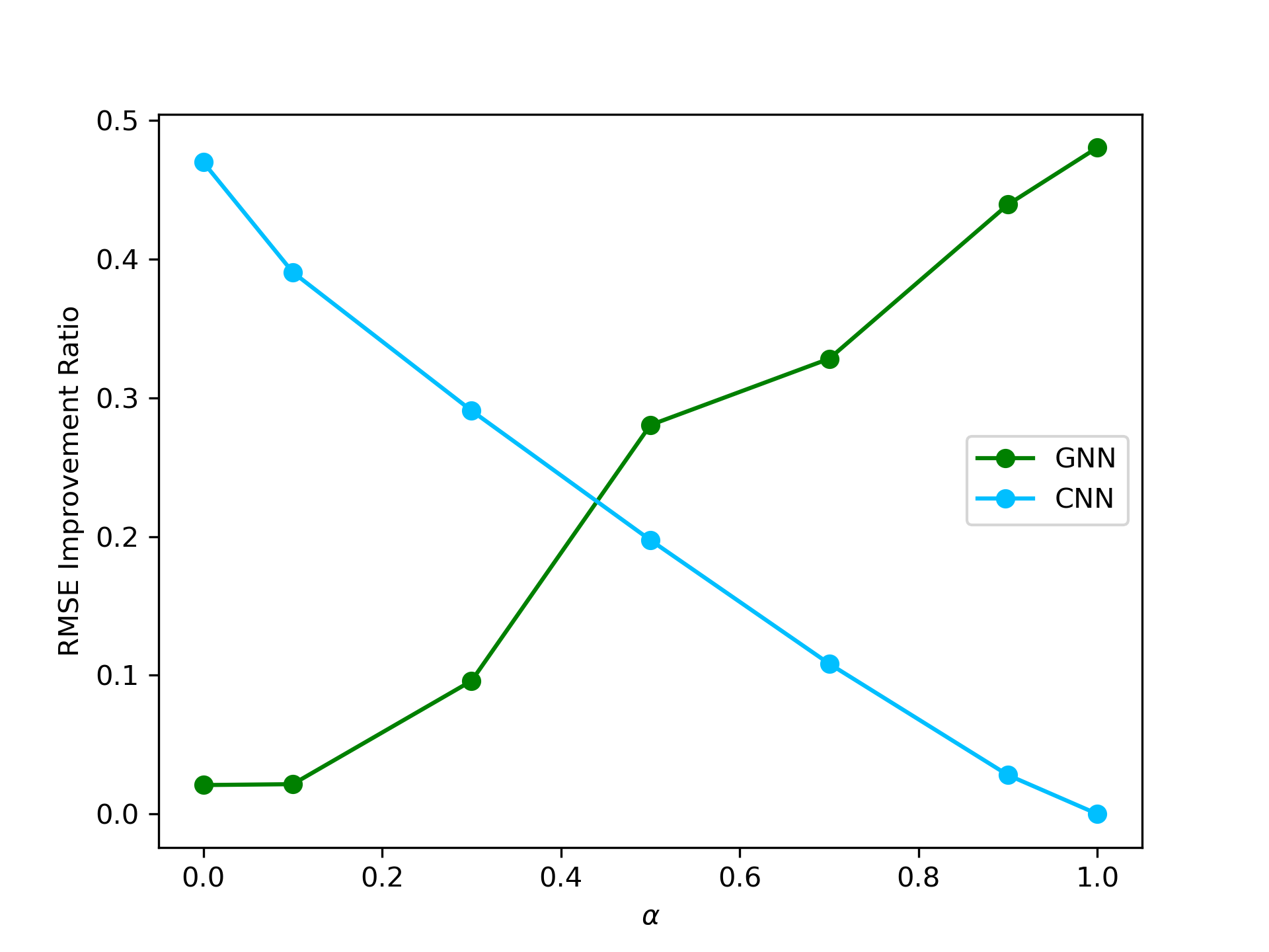
Figure 11: RMSE improvement to to LeNet5 and GIN2 on the test set.

Appendix H Ablation Study

Number of the MLPBlocks.

For MLP fusion scheme, we use GIN and ResNet18 on CRC-MSI to explore the effect of number of MLPBlocks (# MLPBlocks). The image-level AUCs are $75.2\pm 0.85$, $73.4\pm 1.74$, $73.1\pm 0.82$ for # MLPBlocks=1, 2, 3. Consequently, more MLP layers does not contribute to better performance.

Appendix I Related Works

Background for Pathology.

Histology analysis has received much attention, because they are widely considered as the gold standard for cancer diagnosis (Cardesa et al., 2011). The complex patterns and tissue structures presented in histology make manual examination very labor-intensive and time-consuming (Gurcan et al., 2009; Andrion et al., 1995). Even well-experienced experts take a long time to perform careful manual assessments for one slide by observing the histological section under microscopes. With the advent of computational pathology techniques, glass slides are scanned into high-resolution Whole Slide Images (WSIs) for computer-assisted interventions. The remarkable information density of digital histology empowers the complete transition from feature engineering to the usage of deep learning (DL) in mining extensive data. Various applications are developed upon deep learning for histology diagnostic tasks, such as breast cancer segmentation (Cruz-Roa et al., 2014), prostate cancer detection (Litjens et al., 2016), sentinel lymph nodes detection (Litjens et al., 2018).

Background for Biomarker Prediction from Histology.

Biomarkers are defined as clinical indicators for tumor behavior e.g., the responsiveness to therapy or recurrence risk (Duffy, 2013). Identification of biomarkers helps distinguish patients who can benefit from certain molecular therapies (Villalobos and Wistuba, 2017). However, with an increasing amount of biomarkers in oncology workflow, the complexity of treatment recommendations increases tremendously (Kuntz et al., 2021). Furthermore, both the molecular and immunotherapy approaches for biomarker recognition require either additional tissue material or expensive staining dyes, making it cost-intensive and time-consuming. As a ubiquitous image source in real clinical practice that is routinely prepared for cancer diagnosis, histology provides substantive information to be mined. The gene mutations associated with the biomarker rewrite the cellular machinery and change their behavior. Although these morphological changes are subtle to be noticed, empirical results yield that deep learning can directly and reliably detect these features from histology slides. Previous works have shown the effectiveness of deep learning in genetic mutation prediction from non–small cell lung cancer (NSCLC) H&E slides, such as serine/threonine kinase 11 (STK11), tumor protein p53 (TP53), epidermal growth factor receptor (EGFR) (Coudray et al., 2018). Similar to NSCLC, the expression of programmed death-ligand 1 (PD-L1) can be predicted by a multi-field-of-view neural network model (Sha et al., 2019). In prostate cancer, an ensemble of deep neural networks can predict the mutation of BTB/POZ protein (SPOP), achieving a test AUC up to 0.74 (Schaumberg et al., 2018). Another study in melanoma yields that deep learning can predict the NRAS proto-oncogene (NRAS) and B-Raf proto-oncogene (BRAF) from H&E slides (Kim et al., 2020). In terms of microsatellite instability (MSI) or mismatch repair deficiency (dMMR) in colorectal cancer (CRC), following the initial proof of the concept published in 2019 (Kather et al., 2019b), a line of research papers (Cao et al., 2020; Echle et al., 2020; Bilal et al., 2021; Yamashita et al., 2021; Schmauch et al., 2020; Ke et al., 2020) have made much progress.

References

- (1)
- Andrion et al. (1995) A Andrion, Corrado Magnani, PG Betta, et al. 1995. Malignant mesothelioma of the pleura: interobserver variability. Journal of Clinical Pathology 48, 9 (1995), 856.
- Barua et al. (2018) Souptik Barua, Penny Fang, Amrish Sharma, et al. 2018. Spatial interaction of tumor cells and regulatory T cells correlates with survival in non-small cell lung cancer. Lung Cancer 117 (2018), 73–79.
- Bilal et al. (2021) Mohsin Bilal, Shan E Ahmed Raza, Ayesha Azam, Simon Graham, Mohammad Ilyas, Ian A Cree, David Snead, Fayyaz Minhas, and Nasir M Rajpoot. 2021. Novel deep learning algorithm predicts the status of molecular pathways and key mutations in colorectal cancer from routine histology images. MedRxiv (2021).
- Bronstein et al. (2021) Michael M Bronstein, Joan Bruna, Taco Cohen, and Petar Veličković. 2021. Geometric deep learning: Grids, Groups, Graphs, Geodesics, and Gauges. arXiv:2104.13478 (2021).
- Bronstein et al. (2017) Michael M Bronstein, Joan Bruna, Yann LeCun, et al. 2017. Geometric deep learning: going beyond euclidean data. IEEE Signal Processing Magazine 34, 4 (2017), 18–42.
- Calderaro and Kather (2021) Julien Calderaro and Jakob Nikolas Kather. 2021. Artificial intelligence-based pathology for gastrointestinal and hepatobiliary cancers. Gut 70, 6 (2021), 1183–1193.
- Cao et al. (2020) Rui Cao, Fan Yang, Si-Cong Ma, Li Liu, Yu Zhao, Yan Li, De-Hua Wu, Tongxin Wang, Wei-Jia Lu, Wei-Jing Cai, et al. 2020. Development and interpretation of a pathomics-based model for the prediction of microsatellite instability in Colorectal Cancer. Theranostics 10, 24 (2020), 11080.
- Cardesa et al. (2011) Antonio Cardesa, Nina Zidar, Llucia Alos, et al. 2011. The Kaiser’s cancer revisited: was Virchow totally wrong? Virchows Archiv 458, 6 (2011), 649–657.
- Coudray et al. (2018) Nicolas Coudray, Paolo Santiago Ocampo, Theodore Sakellaropoulos, Navneet Narula, Matija Snuderl, David Fenyö, Andre L Moreira, Narges Razavian, and Aristotelis Tsirigos. 2018. Classification and mutation prediction from non–small cell lung cancer histopathology images using deep learning. Nature medicine 24, 10 (2018), 1559–1567.
- Cruz-Roa et al. (2014) Angel Cruz-Roa, Ajay Basavanhally, Fabio González, Hannah Gilmore, Michael Feldman, Shridar Ganesan, Natalie Shih, John Tomaszewski, and Anant Madabhushi. 2014. Automatic detection of invasive ductal carcinoma in whole slide images with convolutional neural networks. In Medical Imaging 2014: Digital Pathology, Vol. 9041. SPIE, 904103.
- Cǎtǎlina et al. (2018) Cangea Cǎtǎlina, Petar Veličković, Nikola Jovanović, et al. 2018. Towards sparse hierarchical graph classifiers. In NeurIPS.
- Dong et al. (2022) Yanni Dong, Quanwei Liu, Bo Du, et al. 2022. Weighted Feature Fusion of Convolutional Neural Network and Graph Attention Network for Hyperspectral Image Classification. IEEE Transactions on Image Processing (2022).
- Duffy (2013) Michael J Duffy. 2013. Tumor markers in clinical practice: a review focusing on common solid cancers. Medical Principles and Practice 22, 1 (2013), 4–11.
- Echle et al. (2020) Amelie Echle, Heike Irmgard Grabsch, Philip Quirke, Piet A van den Brandt, Nicholas P West, Gordon GA Hutchins, Lara R Heij, Xiuxiang Tan, Susan D Richman, Jeremias Krause, et al. 2020. Clinical-grade detection of microsatellite instability in colorectal tumors by deep learning. Gastroenterology 159, 4 (2020), 1406–1416.
- Echle et al. (2021a) Amelie Echle, Narmin Ghaffari Laleh, Peter L Schrammen, Nicholas P West, Christian Trautwein, Titus J Brinker, Stephen B Gruber, Roman D Buelow, Peter Boor, Heike I Grabsch, et al. 2021a. Deep Learning for the detection of microsatellite instability from histology images in colorectal cancer: a systematic literature review. ImmunoInformatics (2021), 100008.
- Echle et al. (2021b) Amelie Echle, Niklas Timon Rindtorff, Titus Josef Brinker, Tom Luedde, Alexander Thomas Pearson, and Jakob Nikolas Kather. 2021b. Deep learning in cancer pathology: a new generation of clinical biomarkers. British Journal of Cancer 124, 4 (2021), 686–696.
- Feichtenbeiner et al. (2014) Anita Feichtenbeiner, Matthias Haas, Maike Büttner, Gerhard G Grabenbauer, Rainer Fietkau, et al. 2014. Critical role of spatial interaction between CD8+ and Foxp3+ cells in human gastric cancer: the distance matters. Cancer Immunology, Immunotherapy 63, 2 (2014), 111–119.
- Fu et al. (2020) Yu Fu, Alexander W Jung, Ramon Viñas Torne, et al. 2020. Pan-cancer computational histopathology reveals mutations, tumor composition and prognosis. Nature Cancer 1, 8 (2020), 800–810.
- Galon et al. (2006) Jérôme Galon, Anne Costes, Fatima Sanchez-Cabo, et al. 2006. Type, density, and location of immune cells within human colorectal tumors predict clinical outcome. Science 313, 5795 (2006), 1960–1964.
- Gilmer et al. (2017) Justin Gilmer, Samuel S Schoenholz, et al. 2017. Neural message passing for quantum chemistry. In ICML.
- Gunduz et al. (2004) Cigdem Gunduz, Bülent Yener, and S Humayun Gultekin. 2004. The cell graphs of cancer. Bioinformatics 20, suppl_1 (2004), i145–i151.
- Gurcan et al. (2009) Metin N Gurcan, Laura E Boucheron, Ali Can, et al. 2009. Histopathological image analysis: A review. IEEE Reviews in Biomedical Engineering 2 (2009), 147–171.
- He et al. (2016) Kaiming He, Xiangyu Zhang, Shaoqing Ren, et al. 2016. Deep residual learning for image recognition. In CVPR.
- Howard et al. (2019) Andrew Howard, Mark Sandler, Grace Chu, et al. 2019. Searching for mobilenetv3. In ICCV.
- Huang et al. (2017) Gao Huang, Zhuang Liu, Laurens Van Der Maaten, et al. 2017. Densely connected convolutional networks. In CVPR.
- Huang et al. (2021) Jinghan Huang, Yiqing Shen, Dinggang Shen, et al. 2021. CA 2.5-Net Nuclei Segmentation Framework with a Microscopy Cell Benchmark Collection. In MICCAI.
- Kather et al. (2019a) Jakob Nikolas Kather, Alexander T Pearson, Niels Halama, et al. 2019a. Deep learning can predict microsatellite instability directly from histology in gastrointestinal cancer. Nature Medicine 25, 7 (2019), 1054–1056.
- Kather et al. (2019b) Jakob Nikolas Kather, Alexander T Pearson, Niels Halama, Dirk Jäger, Jeremias Krause, Sven H Loosen, Alexander Marx, Peter Boor, Frank Tacke, Ulf Peter Neumann, et al. 2019b. Deep learning can predict microsatellite instability directly from histology in gastrointestinal cancer. Nature Medicine 25, 7 (2019), 1054–1056.
- Ke et al. (2020) Jing Ke, Yiqing Shen, Jason D Wright, Naifeng Jing, Xiaoyao Liang, and Dinggang Shen. 2020. Identifying patch-level MSI from histological images of Colorectal Cancer by a Knowledge Distillation Model. In 2020 IEEE International Conference on Bioinformatics and Biomedicine (BIBM). IEEE, 1043–1046.
- Kim et al. (2020) Randie H Kim, Sofia Nomikou, Nicolas Coudray, George Jour, Zarmeena Dawood, Runyu Hong, Eduardo Esteva, Theodore Sakellaropoulos, Douglas Donnelly, Una Moran, et al. 2020. A deep learning approach for rapid mutational screening in melanoma. BioRxiv (2020), 610311.
- Kipf and Welling (2017) Thomas N. Kipf and Max Welling. 2017. Semi-Supervised Classification with Graph Convolutional Networks. In ICLR.
- Kuntz et al. (2021) Sara Kuntz, Eva Krieghoff-Henning, Jakob N Kather, et al. 2021. Gastrointestinal cancer classification and prognostication from histology using deep learning: Systematic review. European Journal of Cancer 155 (2021), 200–215.
- Lambin et al. (2017) Philippe Lambin, Ralph TH Leijenaar, Timo M Deist, et al. 2017. Radiomics: the bridge between medical imaging and personalized medicine. Nature Reviews Clinical Oncology 14, 12 (2017), 749–762.
- LeCun et al. (2015) Yann LeCun, Yoshua Bengio, and Geoffrey Hinton. 2015. Deep learning. Nature 521, 7553 (2015), 436–444.
- Liang et al. (2020) Jiali Liang, Yufan Deng, and Dan Zeng. 2020. A deep neural network combined CNN and GCN for remote sensing scene classification. IEEE Journal of Selected Topics in Applied Earth Observations and Remote Sensing 13 (2020), 4325–4338.
- Liao et al. (2020) Haotian Liao, Yuxi Long, Ruijiang Han, et al. 2020. Deep learning-based classification and mutation prediction from histopathological images of hepatocellular carcinoma. Clinical and Translational Medicine 10, 2 (2020).
- Litjens et al. (2018) Geert Litjens, Peter Bandi, Babak Ehteshami Bejnordi, Oscar Geessink, Maschenka Balkenhol, Peter Bult, Altuna Halilovic, Meyke Hermsen, Rob van de Loo, Rob Vogels, et al. 2018. 1399 H&E-stained sentinel lymph node sections of breast cancer patients: the CAMELYON dataset. GigaScience 7, 6 (2018), giy065.
- Litjens et al. (2016) Geert Litjens, Clara I Sánchez, Nadya Timofeeva, Meyke Hermsen, Iris Nagtegaal, Iringo Kovacs, Christina Hulsbergen-Van De Kaa, Peter Bult, Bram Van Ginneken, and Jeroen Van Der Laak. 2016. Deep learning as a tool for increased accuracy and efficiency of histopathological diagnosis. Scientific Reports 6, 1 (2016), 1–11.
- Lu et al. (2021) Wenqi Lu, Michael Toss, Emad Rakha, Nasir Rajpoot, and Fayyaz Minhas. 2021. SlideGraph+: Whole Slide Image Level Graphs to Predict HER2Status in Breast Cancer. arXiv:2110.06042 (2021).
- Madabhushi and Lee (2016) Anant Madabhushi and George Lee. 2016. Image analysis and machine learning in digital pathology: Challenges and opportunities. Medical Image Analysis 33 (2016), 170–175.
- Monti et al. (2017) Federico Monti, Davide Boscaini, Jonathan Masci, Emanuele Rodola, Jan Svoboda, and Michael M Bronstein. 2017. Geometric deep learning on graphs and manifolds using mixture model CNNs. In CVPR. 5115–5124.
- Noble et al. (2022) Robert Noble, Dominik Burri, Cécile Le Sueur, et al. 2022. Spatial structure governs the mode of tumour evolution. Nature Ecology & Evolution 6, 2 (2022), 207–217.
- Peng et al. (2022) Feifei Peng, Wei Lu, Wenxia Tan, et al. 2022. Multi-Output Network Combining GNN and CNN for Remote Sensing Scene Classification. Remote Sensing 14, 6 (2022), 1478.
- Schaumberg et al. (2018) Andrew J Schaumberg, Mark A Rubin, and Thomas J Fuchs. 2018. H&E-stained whole slide image deep learning predicts SPOP mutation state in prostate cancer. BioRxiv (2018), 064279.
- Schmauch et al. (2020) Benoît Schmauch, Alberto Romagnoni, Elodie Pronier, Charlie Saillard, Pascale Maillé, Julien Calderaro, Aurélie Kamoun, Meriem Sefta, Sylvain Toldo, Mikhail Zaslavskiy, et al. 2020. A deep learning model to predict RNA-Seq expression of tumours from whole slide images. Nature Communications 11, 1 (2020), 1–15.
- Sha et al. (2019) Lingdao Sha, Boleslaw L Osinski, Irvin Y Ho, Timothy L Tan, Caleb Willis, Hannah Weiss, Nike Beaubier, Brett M Mahon, Tim J Taxter, and Stephen SF Yip. 2019. Multi-field-of-view deep learning model predicts nonsmall cell lung cancer programmed death-ligand 1 status from whole-slide hematoxylin and eosin images. Journal of Pathology Informatics 10 (2019).
- Shaban et al. (2019) Muhammad Shaban, Syed Ali Khurram, Muhammad Moazam Fraz, et al. 2019. A novel digital score for abundance of tumour infiltrating lymphocytes predicts disease free survival in oral squamous cell carcinoma. Scientific Reports 9, 1 (2019), 1–13.
- Shen et al. (2017) Dinggang Shen, Guorong Wu, and Heung-Il Suk. 2017. Deep learning in medical image analysis. Annual Review of Biomedical engineering 19 (2017), 221–248.
- Smyth et al. (2021) EC Smyth, V Gambardella, A Cervantes, et al. 2021. Checkpoint inhibitors for gastroesophageal cancers: dissecting heterogeneity to better understand their role in first-line and adjuvant therapy. Annals of Oncology 32, 5 (2021), 590–599.
- Thomas et al. (2013) Aurelien Thomas, Nathan Heath Patterson, Martin M Marcinkiewicz, Anthoula Lazaris, Peter Metrakos, and Pierre Chaurand. 2013. Histology-driven data mining of lipid signatures from multiple imaging mass spectrometry analyses: application to human colorectal cancer liver metastasis biopsies. Analytical Chemistry 85, 5 (2013), 2860–2866.
- Vaswani et al. (2017) Ashish Vaswani, Noam Shazeer, Niki Parmar, et al. 2017. Attention Is All You Need. In NeurIPS.
- Villalobos and Wistuba (2017) Pamela Villalobos and Ignacio I Wistuba. 2017. Lung cancer biomarkers. Hematology/Oncology Clinics 31, 1 (2017), 13–29.
- Wang et al. (2019) Qiang Wang, Bei Li, Tong Xiao, et al. 2019. Learning Deep Transformer Models for Machine Translation. In ACL.
- Wang et al. (2021) Yanan Wang, Yuguang Wang, Changyuan Hu, et al. 2021. Cell graph neural networks enable digital staging of tumour microenvironment and precisely predict patient survival in gastric cancer. medRxiv (2021).
- Wei et al. (2022) Yiran Wei, Chao Li, Xi Chen, et al. 2022. Collaborative learning of images and geometrics for predicting isocitrate dehydrogenase status of glioma. arXiv:2201.05530 (2022).
- Wu et al. (2020) Zonghan Wu, Shirui Pan, Fengwen Chen, et al. 2020. A comprehensive survey on graph neural networks. IEEE TNNLS 32, 1 (2020), 4–24.
- Xu et al. (2018) Keyulu Xu, Weihua Hu, Jure Leskovec, et al. 2018. How powerful are graph neural networks?. In ICLR.
- Yamashita et al. (2021) Rikiya Yamashita, Jin Long, Snikitha Banda, Jeanne Shen, and Daniel L Rubin. 2021. Learning domain-agnostic visual representation for computational pathology using medically-irrelevant style transfer augmentation. IEEE Transactions on Medical Imaging 40, 12 (2021), 3945–3954.
- Yener (2016) Bülent Yener. 2016. Cell-graphs: image-driven modeling of structure-function relationship. Commun. ACM 60, 1 (2016), 74–84.
- Zhang et al. (2020) Ziwei Zhang, Peng Cui, and Wenwu Zhu. 2020. Deep learning on graphs: a survey. IEEE Transactions on Knowledge and Data Engineering (2020).