Unpolarized Transverse Momentum Distributions from a global fit
of Drell-Yan and Semi-Inclusive Deep-Inelastic Scattering data
The MAP Collaboration

Abstract

We present an extraction of unpolarized transverse-momentum-dependent parton distribution and fragmentation functions based on more than two thousand data points from several experiments for two different processes: semi-inclusive deep-inelastic scattering and Drell–Yan production. The baseline analysis is performed using the Monte Carlo replica method and resumming large logarithms at N³LL accuracy. The resulting description of the data is very good ($\chi^{2}/N_{\rm dat}=1.06$). For semi-inclusive deep-inelastic scattering, predictions for multiplicities are normalized by factors that cure the discrepancy with data introduced by higher-order perturbative corrections.

I Introduction

In this paper, we present an extraction of Transverse Momentum Distributions (TMDs) Rogers:2015sqa ; Diehl:2015uka ; Angeles-Martinez:2015sea ; Scimemi:2019mlf using more than two thousand data points from several experiments for two different kinds of processes: Semi-Inclusive Deep Inelastic Scattering (SIDIS) and production of Drell–Yan (DY) lepton pairs, significantly improving our previous analysis Bacchetta:2017gcc .

Building maps of the internal partonic structure of nucleons is a crucial step towards understanding the interactions between quarks and gluons and the phenomenon of confinement. A steady progress in the last decades has led to more and more refined versions of such maps. The TMDs extracted in this article encode information about the three-dimensional distributions of quarks in momentum space. The level of sophistication of a TMD extraction essentially depends on two ingredients: the amount of analyzed data from different processes, namely how “global” the experimental information from which TMDs are extracted, and the perturbative accuracy reached in the theoretical formalism.

The extraction of TMDs is based on TMD factorization theorems, which provide a precise definition of the objects to be extracted, establishing their universality and evolution equations. In this case, the accuracy of the calculation is defined by the amount of large logarithms being resummed, that in turn defines the powers of the strong coupling $\alpha_{s}$ to be included in the perturbative quantities Collins:2011zzd ; Bacchetta:2019sam ; Bozzi:2003jy ; Muselli:2017bad .

Of particular relevance is also the combination of analyzed data from different processes. Similarly to the extraction of collinear Parton Distribution Functions (PDFs), we can talk about a global fit, i.e., a fit that leverages the universality of the parton distributions and uses different processes to constrain them. However, in SIDIS two types of TMDs enter the cross section: the TMD PDFs, describing how partons are arranged in the nucleon, and TMD Fragmentation Functions (FFs), describing how a parton produces a final-state hadron. The knowledge of TMDs, in particular of TMD FFs, would be greatly improved by using data from electron-positron annihilations into two almost back-to-back hadrons Bacchetta:2015ora . Unfortunately, this data is presently not available. There are measurements for the inclusive production of single hadrons Belle:2019ywy but, in this case, transverse momenta need to be defined with respect to the thrust axis: a careful description of the latter is non trivial, and a rigorous factorization theorem for this process has been discussed only recently (see, e.g., Refs. Kang:2020yqw ; Makris:2020ltr ; Boglione:2021wov and references therein). Therefore, for TMD extractions we currently talk about a global fit when data from SIDIS and DY processes are included.

In the last ten years, several extractions of TMDs have been presented Signori:2013mda ; Anselmino:2013lza ; Echevarria:2014xaa ; Sun:2014dqm ; DAlesio:2014mrz ; Bacchetta:2017gcc ; Scimemi:2017etj ; Bertone:2019nxa ; Scimemi:2019cmh ; Bacchetta:2019sam ; Hautmann:2020cyp ; Bury:2022czx . Most of them suffered some shortcomings: they were either obtained in a parton-model framework without QCD corrections, or they took into account only a limited set of data, or did not perform a full fit. TMDs were also studied in a different framework, the so-called parton-branching approach BermudezMartinez:2018fsv ; BermudezMartinez:2019anj ; BermudezMartinez:2020tys .

At present, only two works have reached the stage of combining SIDIS and DY data in a full-fledged global TMD fit: the above mentioned extraction of Ref. Bacchetta:2017gcc , henceforth named PV17, and the extraction of Ref. Scimemi:2019cmh , henceforth named SV19.

The PV17 extraction reached the NLL accuracy, was based on the calculation of observables at mean kinematics in each bin, and did not manage to describe the normalization of all datasets. In this work, we push the accuracy of the analysis to what we will refer to as N³LL^- (only NNLO collinear FFs are currently missing in order to reach full N³LL accuracy). Apart from the increase in perturbative accuracy, in this work we also include many measurements published after 2017.

The SV19 extraction reached the same perturbative accuracy and included essentially the same datasets. Our work has crucial differences in the selection of specific data points (we include a much larger number of points), the implementation of TMD evolution, the choice of nonperturbative components, and the handling of normalization for SIDIS data.

As we will describe in detail, we found it particularly difficult to describe in a satisfactory way the normalization of SIDIS data obtained in fixed-target experiments at moderate to low scales. When the analysis is performed at NLL accuracy, we can describe well shape and normalization of SIDIS data, but the description of high-energy DY data is very poor. Going to N²LL and N³LL^-, the description of DY data significantly improves, but we fail to reproduce the normalization of SIDIS data, mainly due to the ${\cal O}(\alpha_{s})$ corrections to the hard factor. As a possible solution, we choose to adjust the normalization of the TMD predictions by comparing their integral upon transverse momentum and the corresponding collinear formula. With this procedure, we fix the normalization a priori, in a way that is independent of the results of the fit.

Our baseline fit is performed at N³LL^-, using 2031 data points and obtaining $\chi^{2}/N_{\rm dat}=1.06$. We also discuss variations of this baseline fit by changing the theoretical accuracy and the selected data.

The paper is organized as follows. In Sec. II we describe the theoretical framework used in the analysis. In Sec. III we explain how experimental data have been selected. Sec. IV presents the results of our extraction. Finally, in Sec. V we draw our conclusions.

II Formalism

II.1 Drell–Yan

In the Drell–Yan (DY) process

$$h_{A}(P_{A})+h_{B}(P_{B})\ \longrightarrow\ \gamma^{*}/Z(q)+X\longrightarrow\ell^{+}(l)+\ell^{-}(l^{\prime})+X\;,$$ (1)

two hadrons $h_{A}$ and $h_{B}$ with four-momenta $P_{A}$ and $P_{B}$, respectively, collide with center-of-mass energy squared $s=(P_{A}+P_{B})^{2}$, producing a neutral vector boson $\gamma^{*}/Z$ with four-momentum $q$ and large invariant mass $Q=\sqrt{q^{2}}$. The vector boson eventually decays into a lepton and an antilepton with four-momenta constrained by momentum conservation, $q=l+l^{\prime}$. The involved momenta and the respective transverse components are summarized in Fig. 1.

Figure 1: Diagram describing the relevant momenta involved in a DY event. Two partons from two hadrons collide. They have transverse momenta ${\bm{k}_{\perp}}_{A}$ and ${\bm{k}_{\perp}}_{B}$ (not measured). They produce a virtual photon with (measured) transverse momentum $\bm{q}_{T}={\bm{k}_{\perp}}_{A}+{\bm{k}_{\perp}}_{B}$ with respect to the hadron collision axis.

The hadronic four momenta $P_{A}$ and $P_{B}$ can be chosen to identify the longitudinal direction $z$ and define the transverse momentum $\bm{q}_{T}$ of the $\gamma^{*}/Z$. The rapidity of the neutral boson (or, equivalently, of the lepton pair) is defined as

$$y=\frac{1}{2}\ln\left(\frac{q_{0}+q_{z}}{q_{0}-q_{z}}\right)\,.$$ (2)

For our purposes, we need the cross section for this process initiated by unpolarized hadrons and integrated over the azimuthal angle of the exchanged boson. That cross section can be written in terms of two structure functions, $F_{UU}^{1}$ and $F_{UU}^{2}$ Boer:2006eq ; Arnold:2008kf . In the limit $M^{2}\ll Q^{2}$ (with $M$ the mass of the incoming hadrons) and $\bm{q}_{T}^{2}\ll Q^{2}$, the $F_{UU}^{2}$ is suppressed. Accordingly, the cross section reads

$$\frac{d\sigma^{\text{DY/Z}}}{d|\bm{q}_{T}|\,dy\,dQ}=\frac{16\pi^{2}\alpha^{2}}{9Q^{3}}\,|\bm{q}_{T}|\,{\cal P}\,F_{UU}^{1}\big{(}x_{A},x_{B},|\bm{q}_{T}|,Q\big{)}\,,$$ (3)

where $\alpha$ is the electromagnetic coupling, ${\cal P}$ is the phase space factor to account for potential cuts on the lepton kinematics, which turns out to have a relevant impact when high-precision data are taken into account (see, e.g., a recent analysis in Ref. Chen:2022cgv ). At low transverse momentum $\bm{q}_{T}^{2}\ll Q^{2}$, the structure function can be expressed as a convolution over the partonic transverse momenta of two TMD PDFs:

$$\begin{split}F_{UU}^{1}&\big{(}x_{A},x_{B},|\bm{q}_{T}|,Q\big{)}\\ &=x_{A}\,x_{B}\,{\cal H}^{\text{DY}}(Q,\mu)\sum_{a}c_{a}(Q^{2})\int d^{2}{\bm{k}_{\perp}}_{A}\,d^{2}{\bm{k}_{\perp}}_{B}\,f_{1}^{a}(x_{A},{\bm{k}_{\perp}^{2}}_{A};\mu,\zeta_{A})\,f_{1}^{\bar{a}}(x_{B},{\bm{k}_{\perp}^{2}}_{B};\mu,\zeta_{B})\,\delta^{(2)}({\bm{k}_{\perp}}_{A}+{\bm{k}_{\perp}}_{B}-\bm{q}_{T})\\ &=\frac{x_{A}x_{B}}{2\pi}\,{\cal H}^{\text{DY}}(Q,\mu)\sum_{a}c_{a}(Q^{2})\int_{0}^{+\infty}d|\bm{b}_{T}||\bm{b}_{T}|J_{0}\big{(}|\bm{b}_{T}||\bm{q}_{T}|\big{)}\hat{f}_{1}^{a}(x_{A},\bm{b}_{T}^{2};\mu,\zeta_{A})\,\hat{f}_{1}^{\bar{a}}(x_{B},\bm{b}_{T}^{2};\mu,\zeta_{B}).\end{split}$$ (4)

In the above equation, ${\cal H}^{\text{DY}}$ is the hard factor, which can be computed order by order in the strong coupling $\alpha_{s}$ and is equal to 1 at leading order. This function encodes the virtual part of the hard scattering and depends on the hard scale $Q$ and on the renormalisation scale $\mu$. The unpolarized TMDs are denoted by $f_{1}$. They depend on the renormalization scale $\mu$ and the rapidity scale $\zeta$. The rapidity scales must obey the relation $\zeta_{A}\zeta_{B}=Q^{4}$. Throughout the paper, we will set $\mu^{2}=\zeta_{A}=\zeta_{B}=Q^{2}$.

The following definition of the Fourier transform of the TMD PDFs has been used:

$$\begin{split}\hat{f}_{1}^{a}\big{(}x,|\bm{b}_{T}|;\mu,\zeta\big{)}&=\int d^{2}\bm{k}_{\perp}\,e^{i\bm{b}_{T}\cdot\bm{k}_{\perp}}\,f_{1}^{a}\big{(}x,\bm{k}_{\perp}^{2};\mu,\zeta\big{)}\,\\ &=2\pi\int_{0}^{\infty}d|\bm{k}_{\perp}|\,|\bm{k}_{\perp}|J_{0}(|\bm{b}_{T}||\bm{k}_{\perp}|)\,f_{1}^{a}\big{(}x,\bm{k}_{\perp}^{2};\mu,\zeta\big{)}.\,\end{split}$$ (5)

The structure of the TMD PDFs will be addressed in details in Sec. II.3. The transverse momentum of the active quark and antiquark are denoted as ${\bm{k}_{\perp}}_{A,B}$. At low transverse momenta, the two variables $x_{A,B}$ take the values:

$$x_{A} =\frac{Q}{\sqrt{s}}e^{y}\,, x_{B} =\frac{Q}{\sqrt{s}}e^{-y}\,.$$ (6)

The summation over $a$ in Eq. (4) runs over the active quarks and antiquarks at the scale $Q$, and $c_{a}(Q^{2})$ are the respective electroweak charges given by

$$c_{a}(Q^{2})=e_{a}^{2}-2e_{a}V_{a}V_{\ell}\,\chi_{1}(Q^{2})+(V_{\ell}^{2}+A_{\ell}^{2})\,(V_{a}^{2}+A_{a}^{2})\,\chi_{2}(Q^{2})\;,$$ (7)

with

$$\chi_{1}(Q^{2}) =\frac{1}{4\sin^{2}\theta_{W}\cos^{2}\theta_{W}}\frac{Q^{2}(Q^{2}-M_{Z}^{2})}{(Q^{2}-M_{Z}^{2})^{2}+M_{Z}^{2}\Gamma_{Z}^{2}}\;,$$ (8)

$$\chi_{2}(Q^{2}) =\frac{1}{16\sin^{4}\theta_{W}\cos^{4}\theta_{W}}\frac{Q^{4}}{(Q^{2}-M_{Z}^{2})^{2}+M_{Z}^{2}\Gamma_{Z}^{2}}\;,$$ (9)

where $e_{a}$, $V_{a}$, and $A_{a}$ are the electric, vector, and axial charges of the flavor $a$, respectively; $V_{\ell}$ and $A_{\ell}$ are the vector and axial charges of the lepton $\ell$; $\sin\theta_{W}$ is the weak mixing angle; $M_{Z}$ and $\Gamma_{Z}$ are mass and width of the $Z$ boson.

As discussed in Sec. III and summarized in Tab. 2, for DY production the observable provided by the experimental collaborations is the (normalized) cross section differential with respect to $|\bm{q}_{T}|$. For each bin delimited by the initial ($i$) and final ($f$) values of kinematical variables, the experimental values are compared with the following theoretical quantity:

$${\cal O}^{th}_{\text{DY,\,1}}(|\bm{q}_{T}|_{i,f},y_{i,f},Q_{i,f}) =\ \fint_{|\bm{q}_{T}|_{i}}^{|\bm{q}_{T}|_{f}}d|\bm{q}_{T}|\,\int_{y_{i}}^{y_{f}}dy\,\int_{Q_{i}}^{Q_{f}}dQ\,\frac{d\sigma^{\text{DY/Z}}}{d|\bm{q}_{T}|\,dy\,dQ}\,,$$ (10)

where the $\fint$ symbol represents the integral divided by the width of the integration range. Hence, Eq. (10) corresponds to the cross section in Eq. (3) averaged over the transverse momentum and integrated over rapidity and invariant mass of the exchanged boson. The normalized cross section is obtained by dividing both sides of Eq. (10) by the appropriate fiducial cross section, which is computed by employing the ${\tt DYNNLO}$ code Catani:2007vq ; Catani:2009sm .

The low-energy fixed-target experiments included in this analysis (E288, E605, E772, see Tab. 2) measure the following cross section

$$E\,\frac{d\sigma^{\text{DY}}}{d^{3}\bm{q}}=\frac{1}{2\pi\,|\bm{q}_{T}|}\,\frac{d\sigma^{\text{DY}}}{d|\bm{q}_{T}|\,dy},$$ (11)

where $E$ and $\bm{q}$ are the energy and the three-momentum of the photon, respectively.

Given Eq. (11), in principle the experimental value in a given bin needs to be compared against the following theoretical quantity:

$${\cal O}^{th}_{\text{DY,\,ft}}(|\bm{q}_{T}|_{i,f},y_{i,f},Q_{i,f}) =\ \fint_{|\bm{q}_{T}|_{i}}^{|\bm{q}_{T}|_{f}}d|\bm{q}_{T}|\,\fint_{y_{i}}^{y_{f}}dy\,\int_{Q_{i}}^{Q_{f}}dQ\,\frac{1}{2\pi\,|\bm{q}_{T}|}\,\frac{d\sigma^{\text{DY}}}{d|\bm{q}_{T}|\,dy\,dQ}\,.$$ (12)

However, since all the considered fixed-target experiments do not provide bins of $|\bm{q}_{T}|$ but just the average transverse momentum values $|\overline{\bm{q}_{T}}|$, the integration over $|\bm{q}_{T}|$ is not considered. Moreover, the E288 provides only the average value $\overline{y}$ for the rapidity. Accordingly, the theoretical quantity considered for that experiment reads

$${\cal O}^{th}_{\text{DY,\,E288}}(|\overline{\bm{q}_{T}}|,\overline{y},Q_{i,f})=\frac{1}{2\pi\,|\overline{\bm{q}_{T}}|}\,\int_{Q_{i}}^{Q_{f}}dQ\,{\frac{d\sigma^{\text{DY}}}{d|\bm{q}_{T}|\,dy\,dQ}}\bigg{|}_{y=\overline{y},\,|\bm{q}_{T}|=|\overline{\bm{q}_{T}}|}\,.$$ (13)

The E605 and E772 low-energy fixed-target experiments (see Tab. 2) use, in place of the rapidity $y$, the variable $x_{F}$, which is connected to the other kinematic variables as follows:

$$y(x_{F},Q) =\sinh^{-1}\bigg{(}\frac{\sqrt{s}}{Q}\frac{x_{F}}{2}\bigg{)}, x_{A} =\sqrt{\frac{Q^{2}}{s}+\frac{x_{F}^{2}}{4}}+\frac{x_{F}}{2}, x_{B} =x_{A}-x_{F}\,.$$ (14)

Using Eq. (14), one obtains

$$E\,\frac{d\sigma^{\text{DY}}}{d^{3}\bm{q}}=\frac{2E}{\pi\,\sqrt{s}}\,\frac{d\sigma^{\text{DY}}}{d\bm{q}_{T}^{2}\,dx_{F}}\,.$$ (15)

The E772 collaboration provides bins in $x_{F}$ and average transverse momentum values $|\overline{\bm{q}_{T}}|$. Accordingly, in that case the experimental values are compared against the following theoretical quantity:

$${\cal O}^{th}_{\text{DY,\,E772}}(|\overline{\bm{q}_{T}}|,{x_{F}}_{i,f},Q_{i,f}) =\ \int_{Q_{i}}^{Q_{f}}dQ\,\fint_{{x_{F}}_{i}}^{{x_{F}}_{f}}dx_{F}\,\frac{2E}{\pi\,\sqrt{s}}\,\frac{d\sigma^{\text{DY}}}{d\bm{q}_{T}^{2}\,dx_{F}\,dQ}\bigg{|}_{|\bm{q}_{T}|=|\overline{\bm{q}_{T}}|}$$ (16)

$$\approx\frac{\overline{Q}\,\cosh(\overline{y})}{\pi\,|\overline{\bm{q}_{T}}|\,\sqrt{s}\,({x_{F}}_{f}-{x_{F}}_{i})}\,\int_{y({x_{F}}_{i},\overline{Q})}^{y({x_{F}}_{f},\overline{Q})}dy\,\int_{Q_{i}}^{Q_{f}}\,dQ\,\frac{d\sigma^{\text{DY}}}{d|\bm{q}_{T}|\,dy\,dQ}\bigg{|}_{|\bm{q}_{T}|=|\overline{\bm{q}_{T}}|}\,,$$

where

$$\overline{Q} =(Q_{i}+Q_{f})/2\,, \overline{y} =[y({x_{F}}_{i},\overline{Q})+y({x_{F}}_{f},\overline{Q})]/2\,.$$ (17)

For the sake of simplicity, we replaced $y$ and $Q$ with $\overline{y}$ and $\overline{Q}$ in the prefactor in front of the cross section and pull it out of the integral.

The E605 experiment, instead, provides average values for both transverse momentum and $x_{F}$ and its data are compared against the following theoretical quantity:

$${\cal O}^{th}_{\text{DY,\,E605}}(|\overline{\bm{q}_{T}}|,\overline{x_{F}},Q_{i,f}) \approx\frac{\overline{Q}\,\cosh(\overline{y})}{\pi\,|\overline{\bm{q}_{T}}|\,\sqrt{s}}\,\int_{Q_{i}}^{Q_{f}}\,dQ\,\frac{d\sigma^{\text{DY}}}{d|\bm{q}_{T}|\,dy\,dQ}\bigg{|}_{|\bm{q}_{T}|=|\overline{\bm{q}_{T}}|,\,y=\overline{y}}\,,$$ (18)

where, in this case, $\overline{y}=y(\overline{x_{F}},\overline{Q})$ with $\overline{x_{F}}=(x_{Fi}+x_{Ff})/2$.

II.2 Semi-Inclusive Deep-Inelastic Scattering (SIDIS)

In SIDIS, a lepton with momentum $l$ scatters off a hadron target $N$ with mass $M$ and four momentum $P$. In the final state, the scattered lepton momentum $l^{\prime}$ is measured together with one hadron $h$ with mass $M_{h}$ and four momentum $P_{h}$. The other products of the scattering are undetected. Thus the reaction reads

$$\ell(l)+N(P)\rightarrow\ \ell(l^{\prime})+h(P_{h})+X\,.$$ (19)

The (space-like) four-momentum transfer is $q=l-l^{\prime}$, with $Q^{2}\equiv-q^{2}>0$. We use the standard SIDIS variables Bacchetta:2006tn ; Boglione:2019nwk :

$$x =\frac{Q^{2}}{2\,P\cdot q}\,, y =\frac{P\cdot q}{P\cdot l}\,, z =\frac{P\cdot P_{h}}{P\cdot q}\,, \gamma =\frac{2Mx}{Q}\,.$$ (20)

For transverse momenta, we will follow the definitions and notations discussed in Ref. Bacchetta:2004jz ; Boer:2011fh (see also Fig. 2). In particular, we define $\bm{P}_{hT}$ as the hadron transverse momentum in the Breit frame, where $P$ and $q$ form a light-cone basis; as a consequence, $P_{h}$ has only transverse components and $|\bm{P}_{hT}|^{2}=-P_{hT}^{2}$, which is frame independent. Similarly, we define $\bm{q}_{T}$ as the photon transverse momentum in the hadron frame, where $P$ and $P_{h}$ form a light-cone basis; as a consequence, $q_{T}$ has only transverse components and $|\bm{q}_{T}|^{2}=-q_{T}^{2}$, which is also frame independent. The two momenta are related by Bacchetta:2008xw ; Bacchetta:2019qkv

$$q_{T}^{\mu}=-\frac{P^{\mu}_{hT}}{z}-2x\frac{|\bm{q}_{T}|^{2}}{Q^{2}}P^{\mu}\,.$$ (21)

In the following, we will always work assuming that the invariant mass of the photon is large compared to the target and hadron masses ($M^{2},M_{h}^{2}\ll Q^{2}$) and to the transverse momenta $\bm{q}_{T}$ and $\bm{P}_{hT}$ ($\bm{q}_{T}^{2},\,\bm{P}_{hT}^{2}\ll Q^{2}$). We neglect any power corrections that vanish in this limit, both kinematic and dynamical (higher twist), apart from some modifications to the normalization of the SIDIS observables (that could be seen as the effect of power corrections, see Sec. II.4 for more details). In this limit, Eq. (21) reduces to

$$\bm{q}_{T}\approx-\frac{\bm{P}_{hT}}{z}\,.$$ (22)

Several studies have been made concerning higher-twist corrections of various origin (see, e.g., Refs. Mulders:2019mqo ; Boglione:2019nwk ; Accardi:2020iqn for recent works). A careful study of the impact of power corrections to the case of unpolarized TMDs has been discussed in Ref. Scimemi:2019cmh . Lately, important advances in the study of higher-twist TMD factorization have been published Bacchetta:2019qkv ; Vladimirov:2021hdn ; Ebert:2021jhy ; Rodini:2022wki , but they do not directly affect the observables we consider here.

Figure 2: Diagram describing the relevant momenta involved in a SIDIS event in the Breit (nucleon-photon) frame. A virtual photon with momentum $q$ (defining the reference axis) strikes a parton with momentum $k$ inside a nucleon with momentum $P$. The parton has a transverse momentum $\bm{k}_{\perp}$ (not measured). The struck parton with momentum $p=k+q$ fragments into a hadron with momentum $P_{h}$, which acquires a further transverse momentum $\bm{P}_{\perp}$ (not measured) with respect to the fragmenting quark axis. The total measured transverse-momentum of the final hadron is $\bm{P}_{hT}$. When $Q^{2}$ is very large, the longitudinal components are all much larger than the transverse components. In this regime, $\bm{P}_{hT}\approx z\bm{k}_{\perp}+\bm{P}_{\perp}$.

The differential cross section for SIDIS can be witten in terms of two structure functions, $F_{UU,T}$ and $F_{UU,L}$ Bacchetta:2006tn . The subscripts refer to the lepton, the target, and the photon polarization, respectively. The second structure function is formally a twist four contribution and is suppressed in the limit considered here, thus we neglect it. The differential cross section at small transverse momentum Bacchetta:2006tn ; Bacchetta:2017gcc reads

$$\frac{d\sigma^{\text{SIDIS}}}{dx\,dz\,d|\bm{q}_{T}|\,dQ}=\frac{8\pi^{2}\,\alpha^{2}\,z^{2}\,|\bm{q}_{T}|}{x\,Q^{3}}\,\frac{y^{2}}{2(1-\epsilon)}\,\bigg{(}1+\frac{\gamma^{2}}{2x}\bigg{)}\,F_{UU,T}\big{(}x,z,|\bm{q}_{T}|,Q\big{)}\,,$$ (23)

where $\alpha$ is the QED coupling constant and $\epsilon$ is the photon flux factor Bacchetta:2006tn . Neglecting target mass corrections ${\cal O}(\gamma)$ and ${\cal O}(\gamma^{2})$, the prefactors can be approximated as

$$y \approx\frac{Q^{2}}{xs}, \frac{y^{2}}{(1-\epsilon)}\,\bigg{(}1+\frac{\gamma^{2}}{2x}\bigg{)} \approx Y_{+}=1+\bigg{(}1-\frac{Q^{2}}{xs}\bigg{)}^{2}\,.$$ (24)

Since we are interested only in the small-transverse-momentum limit, in Eq. (23) we have neglected the contributions from fixed-order calculations at high $|\bm{q}_{T}|$ Gonzalez-Hernandez:2018ipj ; Wang:2019bvb and the matching of these on TMD factorization Arnold:1990yk ; Collins:2016hqq ; Echevarria:2018qyi .

The unpolarized SIDIS structure function $F_{UU,T}$ is defined as Bacchetta:2006tn

$$\begin{split}F_{UU,T}&\big{(}x,z,|\bm{q}_{T}|,Q\big{)}\\ &=x\,{\cal H}^{\text{S}IDIS}(Q,\mu)\sum_{a}e_{a}^{2}\int d^{2}\bm{k}_{\perp}\,\int\frac{d^{2}\bm{P}_{\perp}}{z^{2}}\,f_{1}^{a}(x,\bm{k}_{\perp}^{2};\mu,\zeta_{A})\,D_{1}^{a\to h}(z,\bm{P}_{\perp}^{2};\mu,\zeta_{B})\,\delta^{(2)}(\bm{k}_{\perp}+\bm{P}_{\perp}/z+\bm{q}_{T})\\ &=\frac{x}{2\pi}\,{\cal H}^{\text{S}IDIS}(Q,\mu)\sum_{a}e_{a}^{2}\int_{0}^{+\infty}d|\bm{b}_{T}||\bm{b}_{T}|J_{0}\big{(}|\bm{b}_{T}||\bm{q}_{T}|\big{)}\hat{f}_{1}^{a}(x,\bm{b}_{T}^{2};\mu,\zeta_{A})\,\hat{D}_{1}^{a\to h}(z,\bm{b}_{T}^{2};\mu,\zeta_{B})\,,\end{split}$$ (25)

where the sum runs over quarks and antiquarks $a$. The hard factor ${\cal H}^{\text{SIDIS}}$ can be computed order by order in the strong coupling $\alpha_{s}$ and is equal to 1 at leading order. The variable $\bm{k}_{\perp}$ is the transverse momentum of the struck quark with respect to the nucleon axis, whereas $\bm{P}_{\perp}$ is the transverse momentum of the produced hadron $h$ with respect to the fragmenting quark axis (see Fig. 2).

The variable $\bm{b}_{T}$ is conjugated via Fourier transform to the transverse momentum $\bm{q}_{T}$. $f_{1}^{a}(x,\bm{k}_{\perp}^{2};\mu,\zeta_{A})$ and $D_{1}^{a\to h}(z,\bm{P}_{\perp}^{2};\mu,\zeta_{B})$ are the unpolarized TMD PDF for a quark $a$ in a nucleon and the unpolarized TMD FF for a quark with flavor $a$ fragmenting into a hadron with flavor $h$, respectively; $\hat{f}_{1}^{a}(x,\bm{b}_{T}^{2};\mu,\zeta_{A})$ and $\hat{D}_{1}^{a\to h}(z,\bm{b}_{T}^{2};\mu,\zeta_{B})$ are their Fourier transforms. The former is defined in Eq.(5), the latter is defined as

$$\begin{split}\hat{D}_{1}^{a\to h}\big{(}z,\bm{b}_{T}^{2};\mu,\zeta\big{)}&=\int\frac{d^{2}\bm{P}_{\perp}}{z^{2}}\,e^{-i\bm{b}_{T}\cdot\bm{P}_{\perp}/z}\,D_{1}^{a}\big{(}z,\bm{P}_{\perp}^{2};\mu,\zeta\big{)}\,\\ &=2\pi\int_{0}^{\infty}\frac{d|\bm{P}_{\perp}|}{z^{2}}\,|\bm{P}_{\perp}|J_{0}(|\bm{b}_{T}||\bm{P}_{\perp}|/z)\,D_{1}^{a}\big{(}z,\bm{P}_{\perp}^{2};\mu,\zeta\big{)}\,.\end{split}$$ (26)

Their structure will be discussed in details in Sec. II.3.

The observable provided by the $\rm HERMES$ and $\rm COMPASS$ collaborations is the multiplicity, namely the ratio of the one-hadron inclusive cross section as a function of the transverse momentum of the hadron $|\bm{P}_{hT}|$ over the fully inclusive one:

$$M(x,z,|\bm{P}_{hT}|,Q)\ =\ \frac{d\sigma^{\text{SIDIS}}}{dx\,dz\,d|\bm{P}_{hT}|\,dQ}\bigg{/}\frac{d\sigma^{\text{DIS}}}{dx\,dQ}=\ \frac{1}{z}\,\frac{d\sigma^{\text{SIDIS}}}{dx\,dz\,d|\bm{q}_{T}|\,dQ}\bigg{/}\frac{d\sigma^{\text{DIS}}}{dx\,dQ}\,.$$ (27)

The cross section for unpolarized DIS in the denominator of the multiplicities reads

$$\frac{d\sigma^{\text{DIS}}}{dx\,dQ}=\frac{8\pi\,\alpha_{s}^{2}}{x\,Q^{3}}\frac{y^{2}}{2(1-\epsilon)}\,\bigg{[}F_{T}(x,Q^{2})+\epsilon F_{L}(x,Q^{2})\bigg{]}\approx\frac{4\pi\,\alpha_{s}^{2}}{x\,Q^{3}}\bigg{[}Y_{+}F_{2}(x,Q^{2})-y^{2}F_{L}(x,Q^{2})\bigg{]}\ ,$$ (28)

where the approximation is justified by neglecting the target mass corrections. At the perturbative order considered in this analysis, the longitudinal DIS structure function $F_{L}$ cannot be neglected, at variance with, e.g., Refs. Signori:2013mda ; Bacchetta:2017gcc .

The experimental values in each bin are compared against the quantity built by separately averaging the numerator and denominator of the multiplicity in Eq. (27) over the respective kinematics:

$${\cal O}^{th}_{\text{SIDIS}}(x_{i,f},z_{i,f},|\bm{P}_{hT}|_{i,f},Q_{i,f}) =\fint_{Q_{i}}^{Q_{f}}dQ\,\fint_{x_{i}}^{x_{f}}dx\,\fint_{z_{i}}^{z_{f}}dz\,\fint_{|\bm{P}_{hT}|_{i}}^{|\bm{P}_{hT}|_{f}}d|\bm{P}_{hT}|\ \frac{d\sigma^{\text{SIDIS}}}{dx\,dz\,d|\bm{P}_{hT}|\,dQ}\ ,$$ (29)

$${\cal O}^{th}_{\text{DIS}}(x_{i,f},Q_{i,f}) =\fint_{Q_{i}}^{Q_{f}}dQ\,\fint_{x_{i}}^{x_{f}}dx\ \frac{d\sigma^{\text{DIS}}}{dx\,dQ}\ ,$$

$${\cal M}^{th}(x_{i,f},z_{i,f},|\bm{P}_{hT}|_{i,f},Q_{i,f}) ={\cal O}^{th}_{\text{SIDIS}}(x_{i,f},z_{i,f},|\bm{P}_{hT}|_{i,f},Q_{i,f})\bigg{/}{\cal O}^{th}_{\text{DIS}}(x_{i,f},Q_{i,f})\ .$$ (30)

The $\rm HERMES$ collaboration provides multiplicities in bins of $|\bm{P}_{hT}|$, whereas the $\rm COMPASS$ collaboration in bins of $\bm{P}_{hT}^{2}$ (see also Tab. 3). In both cases, the observable can be calculated as in Eq. (29), but in the $\rm COMPASS$ case the average is on $\bm{P}_{hT}^{2}$. Moreover, both collaborations introduce a cut on the invariant mass of the hadronic final states $W^{2}=(P+q)^{2}$ (see Tab. 3), which makes the upper integration limit $x_{f}$ a $Q$-dependent quantity.

II.3 Transverse Momentum Distributions (TMDs)

As a consequence of the renormalization of ultraviolet and rapidity divergences Collins:2011zzd ; Echevarria:2011epo ; Grewal:2020hoc , TMD PDFs and FFs acquire a dependence on the renormalization scale $\mu$ and on the rapidity scale $\zeta$. The evolution of TMDs from some initial values of the scales $\mu_{i}$, $\zeta_{i}$, to some final values $\mu_{f},\zeta_{f}$, is given by

$$\hat{f}_{1}^{a}(x,\bm{b}_{T}^{2};\mu_{f},\zeta_{f})=\hat{f}_{1}^{a}(x,\bm{b}_{T}^{2};\mu_{i},\zeta_{i})\,\exp\bigg{\{}\int_{\mu_{i}}^{\mu_{f}}\frac{d\mu}{\mu}\,\gamma\big{(}\mu,\zeta_{f}\big{)}\bigg{\}}\,\bigg{(}\frac{\zeta_{f}}{\zeta_{i}}\bigg{)}^{K(|\bm{b}_{T}|,\,\mu_{i})/2}\,.$$ (31)

The anomalous dimension $\gamma$ for the renormalization-group evolution in $\mu$ reads:

$$\gamma\big{(}\mu,\zeta\big{)}=\gamma_{F}\big{(}\alpha_{s}(\mu)\big{)}-\gamma_{K}\big{(}\alpha_{s}(\mu)\big{)}\,\ln\,\frac{\sqrt{\zeta}}{\mu}\,,$$ (32)

where $\gamma_{K}$ is the cusp anomalous dimension and $\gamma_{F}\big{(}\alpha_{s}(\mu)\big{)}=\gamma\big{(}\mu,\mu^{2}\big{)}$ is the boundary condition Bacchetta:2019sam . The Collins–Soper kernel $K$, instead, is the anomalous dimension for the evolution in $\zeta$ Collins:2011zzd . The same structure holds for the TMD FF. In order to avoid the insurgence of large logarithms, the scales $\mu_{i}$ and $\zeta_{i}$ are conveniently fixed as $\mu_{i}=\sqrt{\zeta_{i}}=\mu_{b}=2e^{-\gamma_{E}}/|\bm{b}_{T}|$. Since the coupling $\alpha_{s}$ is computed at this scale (see Eq. (32)) the evolution of the TMD is perturbatively meaningful only at low values of $|\bm{b}_{T}|$ such that the scale $\mu_{b}$ is sufficiently larger than the Landau pole $\Lambda_{\rm QCD}$. This condition can be implemented by replacing the scale $\mu_{b}$ with $\mu_{b_{*}}=2e^{-\gamma_{E}}/{b_{*}}$, where Bacchetta:2017gcc

$$b_{*}(|\bm{b}_{T}|,b_{\text{min}},b_{\text{max}})=b_{\text{max}}\,\bigg{(}\frac{1-e^{-|\bm{b}_{T}|^{4}/b_{\text{max}}^{4}}}{1-e^{-|\bm{b}_{T}|^{4}/b_{\text{min}}^{4}}}\bigg{)}^{1/4}\,,$$ (33)

with

$$b_{\text{max}} =2e^{-\gamma_{E}}\text{ GeV}^{-1}\approx 1.123\text{ GeV}^{-1}\,, b_{\text{min}} =2e^{-\gamma_{E}}/\mu_{f}\ .$$ (34)

As suggested by the CSS formalism Collins:2011zzd , $b_{*}$ saturates to $b_{\text{max}}$ at large $|\bm{b}_{T}|$ guaranteeing that $\mu_{b_{*}}$ never enters the nonperturbative regime. However, this has also the effect of introducing power corrections scaling like $(\Lambda_{\rm QCD}/|\bm{q}_{T}|)^{k}$ Catani:1996yz , with $k>0$, that in the region $|\bm{q}_{T}|\simeq\Lambda_{\rm QCD}$ need to be accounted for by a nonperturbative function. At small $|\bm{b}_{T}|$, $b_{*}$ saturates to $b_{\text{min}}$. Since $\mu_{f}$ is of the order of the boson virtuality $Q$, this introduces subleading power corrections scaling like $(|\bm{q}_{T}|/Q)^{n}$, with $n>0$. Such a procedure has the advantage of facilitating a possible matching of the TMD formula, valid for $|\bm{q}_{T}|\ll Q$, onto the fixed-order calculation valid for $|\bm{q}_{T}|\simeq Q$ Bozzi:2003jy ; Bozzi:2005wk ; Bizon:2018foh . Accordingly, in the limit $|\bm{b}_{T}|\to 0$ the Sudakov exponent vanishes.

Performing at the input scales the Operator Product Expansion (OPE) of the TMD PDFs (TMD FFs) around $|\bm{b}_{T}|=0$ one gets:

$$\hat{f}_{1}^{a}(x,b_{*};\mu_{b_{*}},\mu_{b_{*}}^{2})=\sum_{b}\,\int_{x}^{1}\frac{dx^{\prime}}{x^{\prime}}\,C^{ab}(x^{\prime},b_{*};\mu_{b_{*}},\mu_{b_{*}}^{2})\,f_{1}^{b}\bigg{(}\frac{x}{x^{\prime}};\mu_{b_{*}}\bigg{)}\equiv[C\otimes f_{1}](x,b_{*};\mu_{b_{*}},\mu_{b_{*}}^{2})\,,$$ (35)

where the sum runs over quarks, antiquarks, and the gluon. The matching coefficients $C$ are calculated as a perturbative expansion in powers of $\alpha_{s}$.

In view of the power corrections introduced by the $b_{*}$ prescription, both the Collins–Soper kernel $K$ Grewal:2020hoc and the OPE in Eq. (35) need to be modified to account for nonperturbative effects. For the Collins–Soper kernel $K$, this results in a nonperturbative correction term, $g_{K}(\bm{b}_{T}^{2})$, for which we choose a specific functional form:

$$K(|\bm{b}_{T}|,\mu_{b_{*}})=K(b_{*},\mu_{b_{*}})+g_{K}(|\bm{b}_{T}|)\,, g_{K}(\bm{b}_{T}^{2})=-g_{2}^{2}\,\frac{\bm{b}_{T}^{2}}{2}\,.$$ (36)

This correction gives rise in the evolution to a nonperturbative factor that goes like $(\zeta_{f}/Q_{0}^{2})^{g_{K}/2}$ where $Q_{0}$ is an arbitrary scale at which this correction is parameterised; we set $Q_{0}=1$ GeV. In order not to affect the perturbative calculation at small $|\bm{b}_{T}|$, the term $g_{K}$ needs to vanish in the limit $|\bm{b}_{T}|\to 0$. The nonperturbative corrections to the OPE can also be parameterised by a multiplicative function that generally depends on $x$ or $z$ and $\bm{b}_{T}$. The net result of the inclusion of the nonperturbative corrections into the evolved TMD PDF reads:

$$\hat{f}_{1}^{a}(x,\bm{b}_{T}^{2};\mu_{f},\zeta_{f})=[C\,\otimes\,f_{1}](x,b_{*};\mu_{b_{*}},\mu_{b_{*}}^{2})\,\exp\bigg{\{}\int_{\mu_{b_{*}}}^{\mu_{f}}\frac{d\mu}{\mu}\,\gamma\big{(}\mu,\zeta_{f}\big{)}\bigg{\}}\,\bigg{(}\frac{\zeta_{f}}{\mu_{b_{*}}^{2}}\bigg{)}^{K(b_{*},\,\mu_{b_{*}})/2}\,f_{1\,NP}(x,\bm{b}_{T}^{2};\zeta_{f},Q_{0})\,,$$ (37)

and the same holds for the TMD FF where one introduces $D_{1\,NP}(z,\bm{b}_{T}^{2};\zeta,Q_{0})$. Note that the number of active flavors $n_{f}$ in the perturbative quantities $\gamma$, $C$, and the hard function ${\cal H}$ of Eqs. (4) and (25), is separately determined by the scales $\mu$, $\mu_{b_{*}}$ and $Q$, respectively. To be more precise, given a set of quark thresholds $\{m_{1},m_{2},m_{3},\dots\}$, the $n_{f}$ associated to each of the three scales above is computed by requiring that the scale lies between $m_{n_{f}}$ and $m_{n_{f}+1}$. Analogously, since the collinear distributions involved in the matching formula in Eq. (35) are computed at the scale $\mu_{b_{*}}$, the value of $n_{f}$ for PDFs and FFs is chosen accordingly, i.e. it is the same used for the matching functions $C$.

The $f_{1\,NP}$ and $D_{1\,NP}$ factors (which we assume to be flavor-independent) incorporate both the correction to the evolution associated to the $g_{K}$ function and the correction to the respective OPE. For the TMD PDF we define

$$f_{1\,NP}(x,\bm{b}_{T}^{2};\zeta,Q_{0})=\frac{g_{1}(x)\,e^{-g_{1}(x)\frac{\bm{b}_{T}^{2}}{4}}+\lambda^{2}\,g_{1B}^{2}(x)\,\bigg{[}1-g_{1B}(x)\frac{\bm{b}_{T}^{2}}{4}\bigg{]}\,e^{-g_{1B}(x)\frac{\bm{b}_{T}^{2}}{4}}+\lambda_{2}^{2}\,g_{1C}(x)\,e^{-g_{1C}(x)\frac{\bm{b}_{T}^{2}}{4}}}{g_{1}(x)+\lambda^{2}\,g_{1B}^{2}(x)+\lambda_{2}^{2}\,g_{1C}(x)}\,\bigg{[}\frac{\zeta}{Q_{0}^{2}}\bigg{]}^{g_{K}(\bm{b}_{T}^{2})/2}\,,$$ (38)

and for the TMD FF the form is

$$D_{1\,NP}(z,\bm{b}_{T}^{2};\zeta,Q_{0})=\frac{g_{3}(z)\,e^{-g_{3}(z)\frac{\bm{b}_{T}^{2}}{4z^{2}}}+\frac{\lambda_{F}}{z^{2}}\,g_{3B}^{2}(z)\,\bigg{[}1-g_{3B}(z)\frac{\bm{b}_{T}^{2}}{4z^{2}}\bigg{]}\,e^{-g_{3B}(z)\frac{\bm{b}_{T}^{2}}{4z^{2}}}}{g_{3}(z)+\frac{\lambda_{F}}{z^{2}}\,g_{3B}^{2}(z)}\,\bigg{[}\frac{\zeta}{Q_{0}^{2}}\bigg{]}^{g_{K}(\bm{b}_{T}^{2})/2}\,.$$ (39)

The nonperturbative factors $f_{1\,NP}$, $D_{1\,NP}\to 1$ for $\bm{b}_{T}\to 0$. The $g_{i}$ functions describe the dependence of the widths of the distributions on $x$ and $z$:

$$g_{\{1,1B,1C\}}(x)=N_{\{1,1B,1C\}}\frac{x^{\sigma_{\{1,2,3\}}}(1-x)^{\alpha^{2}_{\{1,2,3\}}}}{\hat{x}^{\sigma_{\{1,2,3\}}}(1-\hat{x})^{\alpha^{2}_{\{1,2,3\}}}}\,,$$ (40)

$$g_{\{3,3B\}}(z)=N_{\{3,3B\}}\frac{(z^{\beta_{\{1,2\}}}+\delta^{2}_{\{1,2\}})(1-z)^{\gamma^{2}_{\{1,2\}}}}{(\hat{z}^{\beta_{\{1,2\}}}+\delta^{2}_{\{1,2\}})(1-\hat{z})^{\gamma^{2}_{\{1,2\}}}}\,,$$ (41)

where $\hat{x}=0.1$, $\hat{z}=0.5$.

In total, the default configuration for the fit involves 21 free parameters: one associated to the nonperturbative part of the Collins–Soper kernel (Eq. (36)), 11 related to the nonperturbative part of the TMD PDF (Eqs. (38), (40)), and 9 for the nonperturbative part of the TMD FF (Eqs. (39), (41)).

The functional forms in Eqs. (38)-(41) are largely arbitrary. However, an important feature is that they are the Fourier transforms of the sum of a Gaussian, a weighted Gaussian (multiplied by $\bm{k}_{\perp}^{2}$) and, in the case of the TMD PDFs, a third Gaussian. They are therefore positive definite for all values of $\bm{k}_{\perp}^{2}$. The parameters $\lambda$ and $\lambda_{2}$ in Eq. (38) are squared in order to avoid negative contributions (there is no need to square the parameter $\lambda_{F}$ in Eq. (39) because the fit always selects positive values for this parameter). The widths of the Gaussians, expressed by Eqs. (40), (41), are $x$ (or $z$) dependent and vanish as $x$ (or $z$) approaches 1. Our choice of the functional form is also inspired by model calculations of TMD PDFs (see, e.g., Bacchetta:2008af ; Pasquini:2008ax ; Avakian:2010br ; Burkardt:2015qoa ; Gutsche:2016gcd ; Maji:2017bcz ; Alessandro:2021cbg ; Signal:2021aum ) and TMD FFs (see, e.g, Bacchetta:2007wc ; Matevosyan:2011vj ). Many of these models predict the existence of terms that behave similarly to Gaussians and weighted Gaussians. The details of the functional dependence predicted by the models are related to the correlation between the spin of the quarks and their transverse momentum. In the case of fragmentaton functions, a different role can be played by different producton channels (e.g., direct production vs. production through the decay of hadronic resonances).

Finally, for the logarithmic ordering we use the same convention adopted in Ref. Bacchetta:2019sam . In particular, the orders of truncation of the perturbative ingredients relevant to the present analysis are summarized in Tab. 1. At the time of this analysis, the full N³LL accuracy could not be achieved because NNLO collinear FFs were not available. Very recently, two analyses of collinear FFs were presented in Refs. Borsa:2022vvp ; Khalek:2022vgy making an extraction of TMDs at full N³LL possible. We leave this study to a future pubblication.

Accuracy	$H$ and $C$	$K$ and $\gamma_{F}$	$\gamma_{K}$	PDF and $\alpha_{s}$ evolution	FF evolution
NLL	0	1	2	LO	LO
N2LL	1	2	3	NLO	NLO
N3LL-	2	3	4	NNLO	NLO
N3LL	2	3	4	NNLO	NNLO

Table 1: Truncation orders in the expansions of the perturbative ingredients of TMDs relevant to the logarithmic counting considered in this paper (see text). The last column refers to the order used for the evolution of the collinear FFs.

II.4 Normalization factors for SIDIS

In Ref. Bacchetta:2017gcc it was demonstrated that TMD factorization at NLL accuracy is able to successfully reproduce the normalization and shape of $\rm HERMES$ SIDIS multiplicities and the shape of the available $\rm COMPASS$ multiplicities. More recently, the $\rm COMPASS$ collaboration published a reanalysis of their data COMPASS:2017mvk . The NLL TMD predictions correctly reproduce normalization and shape of the new data Piacenza:2020sst . However, when increasing the accuracy to N²LL or higher, the TMD formula severely underestimates the measurements OsvaldoGonzalez-Hernandez:2019iqj ; Piacenza:2020sst by nearly constant factors in each bin. Note that tensions between the TMD cross sections and the associated measurements exist also at large transverse momentum in SIDIS Gonzalez-Hernandez:2018ipj , DY Bacchetta:2019tcu , and electron-positron annihilation into two hadrons Moffat:2019pci .

In the present study, as will be shown in Sec. IV, we confirm that we obtain an excellent description of both normalization and shape of the SIDIS multiplicities at NLL and that the N²LL results are much smaller. At N³LL the results increase slightly, but they are still far from the NLL ones and, therefore, from data. At average kinematics of the $\rm COMPASS$ measurements, we obtain the following ratios of multiplicities:

$$\frac{M_{\rm NLL}}{M_{\rm N^{2}LL}} \gtrsim 2, \frac{M_{\rm NLL}}{M_{\rm N^{3}LL}} \gtrsim 1.5.$$ (42)

The reason for the difference between the logarithmic orders is almost entirely due to the hard factor in Eq. (25) Collins:2017oxh . If we look at the explicit expression for the hard factor with the standard choice $\mu=Q$

$${\cal H}^{\rm SIDIS}(Q,Q)=1+\frac{\alpha_{s}(Q)}{4\pi}C_{F}\bigg{(}-16+\frac{\pi^{2}}{3}\bigg{)},$$ (43)

we can immediately see that just by introducing ${\cal O}(\alpha_{s})$ corrections, at $Q=2$ GeV with $\alpha_{s}\approx 0.3$, we reduce the structure function to about 60% of its original value. This change is not compensated by a similar reduction in the denominator of Eq. (27): the differences between the LO and NLO expressions of the inclusive DIS cross section are typically below 5% and the NLO results are actually larger than the LO ones.

If the NLL expression is much larger than the N²LL and N³LL ones, we may suspect that it should overshoot the data by a factor 1.5 at least. However, several works before the present one have shown a good agreement with data using a parton-model approach Signori:2013mda ; Anselmino:2013lza or at NLL Echevarria:2014xaa ; Sun:2014dqm . Moreover, the integral of the structure function over $\bm{q}_{T}$ is equal to the value of its Fourier transform at $\bm{b}_{T}=0$. Using any $b^{*}$ prescription with $b_{\rm min}=2e^{-\gamma_{E}}/Q$, the integral of the NLL expression by construction corresponds to the LO expression of the collinear SIDIS structure function, independent of the TMD nonperturbative parameters:

$$\begin{split}\int d^{2}\bm{q}_{T}\,F_{UU,T}\big{(}x,z,|\bm{q}_{T}|,Q\big{)}&=x\,\sum_{a}e_{a}^{2}\,{\cal H}^{\rm SIDIS}(Q,Q)\bigg{(}\hat{f}_{1}^{a}(x,\bm{b}_{T}^{2};Q,Q^{2})\,\hat{D}_{1}^{a\to h}(z,\bm{b}_{T}^{2};Q,Q^{2})\bigg{)}\bigg{|}_{|\bm{b}_{T}|=0}\\ &\stackrel{{\scriptstyle\rm NLL}}{{=}}x\,\sum_{a}e_{a}^{2}\,{f}_{1}^{a}(x;Q)\,{D}_{1}^{a\to h}(z;Q).\end{split}$$ (44)

The LO collinear SIDIS predictions are known to describe the data reasonably well and, if anything, they seem to be lower than the data deFlorian:2007aj ; HERMES:2012uyd . Therefore, the integral of our NLL expression is in good agreement with data, which also indicates the absence of a large normalization error.

If the NLL predictions describe the data well and are a factor 2 or 1.5 above the N²LL and N³LL predictions, we propose to modify the normalization of the latter to recover a good agreement with data. An extended discussion of this issue can be found in Ref. Piacenza:2020sst . We observe that the integral of the TMD formula, valid at low $\bm{q}_{T}$, should reproduce only part of the full collinear cross section. The only exception is the order ${\cal O}(\alpha_{s}^{0})$ case, as we have seen above, since at that order there is no contribution from gluon radiation at high transverse momentum, beyond the TMD region.

However, at N²LL or higher, in the kinematics of fixed-target SIDIS experiments, the integral of the TMD region (i.e., the integral of the so-called $W$ term in the language of Ref. Collins:2011zzd ) is much smaller than the corresponding collinear cross section. The missing contribution to the integral should be recovered by the terms in the fixed-order calculation that are not included in the TMD resummed expression (the so-called $Y$ term). Ideally, the $Y$ term should be negligible in the low-$\bm{q}_{T}$ region. This is not the case in the experimental regions under consideration: the $Y$ term is finite but relatively large, even at $\bm{q}_{T}=0$.

If we consider the contribution to the integral of the $W$ term (i.e., the integral of Eq. (23)), with our $b_{\rm min}$ prescription, at order $\alpha_{s}$ we obtain, schematically

$$\int d^{2}\bm{q}_{T}\,W\biggr{|}_{{\cal O}(\alpha_{s})}=\sigma_{0}\frac{\alpha_{s}}{4\pi}\sum_{q}e_{q}^{2}\Bigl{[}D_{1}^{q\to h}\otimes C_{\rm TMD}^{qq}\otimes f_{1}^{q}+D_{1}^{q\to h}\otimes C_{\rm TMD}^{qg}\otimes f_{1}^{g}+D_{1}^{g\to h}\otimes C_{\rm TMD}^{gq}\otimes f_{1}^{q}\Bigr{]}(x,z,Q),$$ (45)

where

$$\sigma_{0}=\frac{4\pi^{2}\,\alpha^{2}\,z^{2}\,|\bm{q}_{T}|}{x\,Q^{3}}Y_{+}.$$ (46)

The double convolution over both $x$ and $z$ is defined as

$$\Bigl{[}D_{1}^{a\to h}\otimes C^{ab}\otimes f_{1}^{b}\Bigr{]}(x,z,Q)=\frac{1}{z^{2}}\int_{x}^{1}\frac{dx^{\prime}}{x^{\prime}}\int_{z}^{1}\frac{dz^{\prime}}{z^{\prime}}D_{1}^{a\to h}(z^{\prime};Q)C^{ab}\Bigl{(}\frac{x}{x^{\prime}},\frac{z}{z^{\prime}}\Bigr{)}f_{1}^{b}(x^{\prime};Q)$$ (47)

and the $C_{\rm TMD}$ coefficients can be found in App. A.

The integral in Eq. (45) should be compared to the collinear expression at the same order (see, e.g., Ref. deFlorian:1997zj )

$$\begin{split}\frac{d\sigma^{\text{SIDIS}}}{dxdQdz}\biggr{|}_{{\cal O}(\alpha_{s})}&=\sigma_{0}\frac{\alpha_{s}}{4\pi}\sum_{q}e_{q}^{2}\biggl{\{}\Bigl{[}D_{1}^{q\to h}\otimes C_{1}^{qq}\otimes f_{1}^{q}+D_{1}^{q\to h}\otimes C_{1}^{qg}\otimes f_{1}^{g}+D_{1}^{g\to h}\otimes C_{1}^{gq}\otimes f_{1}^{q}\Bigr{]}(x,z,Q)\\ &\quad+\frac{1-y}{1+(1-y)^{2}}\Bigl{[}D_{1}^{q\to h}\otimes C_{L}^{qq}\otimes f_{1}^{q}+D_{1}^{q\to h}\otimes C_{L}^{qg}\otimes f_{1}^{g}+D_{1}^{g\to h}\otimes C_{L}^{gq}\otimes f_{1}^{q}\Bigr{]}(x,z,Q)\biggr{\}}.\\ \end{split}$$ (48)

The QCD coefficients $C_{1}^{ab}$ and $C_{L}^{ab}$ are calculated in perturbation theory. The former can be written as

$$C_{1}^{ab}(x,z;Q,\mu) =C_{\rm nomix}^{ab}(x,z,Q,\mu)+C_{\rm mix}^{ab}(x,z).$$ (49)

The coefficient $C_{\rm nomix}$ is the sum of all those terms that contain either a $\delta(1-x)$ or a $\delta(1-z)$ (or both). Some of these terms are present in $C_{\rm TMD}$, but not all. This definition holds at all orders in $\alpha_{s}$. The $C_{L}$ matching coefficients, instead, only contain “mixed” contributions. For convenience, we reproduce all coefficients at order $\alpha_{s}$ in App. A.

In order to increase the size of the TMD component, we consider the contribution of all the “nonmixed” terms $C_{\rm nomix}$. The reason behind this choice is that it might be possible to include such terms into a redefinition of the individual TMDs. Hence, we define

$$\frac{d\sigma^{\rm nomix}}{dxdQdz}\biggr{|}_{{\cal O}(\alpha_{s})}=\sigma_{0}\frac{\alpha_{s}}{4\pi}\sum_{q}e_{q}^{2}\Bigl{[}D_{1}^{q\to h}\otimes C_{\rm nomix}^{qq}\otimes f_{1}^{q}+D_{1}^{q\to h}\otimes C_{\rm nomix}^{qg}\otimes f_{1}^{g}+D_{1}^{g\to h}\otimes C_{\rm nomix}^{gq}\otimes f_{1}^{q}\Bigr{]}(x,z,Q),$$ (50)

and similarly for higher orders, and we introduce the following normalization factor:

$$\omega(x,z,Q)=\frac{d\sigma^{\rm nomix}}{dx\,dz\,dQ}\bigg{/}\int d^{2}\bm{q}_{T}\,W\,.$$ (51)

We stress that these normalization factors depend only on the collinear PDFs and FFs, are independent of the parametrization of the nonperturbative part of the TMDs, and can be computed before performing a fit of the latter.

At NLL, $\omega(x,z,Q)=1$. Beyond NLL, the prefactor becomes larger than one and guarantees that the integral of the TMD part of the cross section reproduces most of the collinear cross section, as suggested by the data. On the contrary, without the enhancement due to the normalization factor, the integral of the TMD part of the cross section would be too small, requiring a large role of the high-transverse-momentum tail, which is not observed in the data. The impact of the normalization factor defined in Eq. (51) will be addressed in detail in Sec. IV.

As a consequence of our procedure, the theoretical expression for the SIDIS cross section in Eq. (23) becomes

$$\frac{d\sigma_{\omega}^{\text{SIDIS}}}{dx\,dz\,d|\bm{q}_{T}|\,dQ}=\omega(x,z,Q)\,\frac{d\sigma^{\text{SIDIS}}}{dx\,dz\,d|\bm{q}_{T}|\,dQ}\,.$$ (52)

III Data selection

In this Section we describe the experimental data included in our global analysis. We consider a large number of datasets related to DY lepton pair production and SIDIS, for the observables discussed in Sec. II.1 and Sec. II.2. The coverage in the $x$-$Q^{2}$ plane spanned by these datasets is illustrated in Fig. 3.

The majority of datasets analyzed in the present work was already included in the global analysis of SIDIS and DY data in Ref. Bacchetta:2017gcc and in the fit of DY data discussed in Ref. Bacchetta:2019sam . For more details, we refer the reader to those references. The new datasets included in the present analysis are:

• DY di-muon production from the collision of a proton beam with an energy of 800 GeV on a ${}^{2}H$ fixed target from E772 ($\sqrt{s}=38.8$ GeV) E772:1994cpf ;

• DY di-muon production from the PHENIX Collaboration PHENIX:2018dwt ;

• DY data at 13 TeV from the CMS Collaboration CMS:2019raw and the ATLAS Collaboration ATLAS:2019zci .

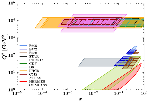
Figure 3: The $x$ vs. $Q^{2}$ coverage spanned by the experimental data considered in this analysis (see also Tab. 2 and Tab. 3).

III.1 Drell-Yan

Our analysis is based on TMD factorization, which is applicable only in the region $|\bm{q}_{T}|\ll Q$. Therefore, in agreement with the choices of Refs. Bacchetta:2019sam ; Scimemi:2019cmh we impose the following cut

$$|\bm{q}_{T}|<0.2\,Q\,.$$ (53)

Experiment	$N_{\rm dat}$	Observable	$\sqrt{s}$ [GeV]	$Q$ [GeV]	$y$ or $x_{F}$	Lepton cuts	Ref.
E605	50	$Ed^{3}\sigma/d^{3}\bm{q}$	38.8	7 - 18	$x_{F}=0.1$	-	Moreno:1990sf
E772	53	$Ed^{3}\sigma/d^{3}\bm{q}$	38.8	5 - 15	$0.1<x_{F}<0.3$	-	E772:1994cpf
E288 200 GeV	30	$Ed^{3}\sigma/d^{3}\bm{q}$	19.4	4 - 9	$y=0.40$	-	Ito:1980ev
E288 300 GeV	39	$Ed^{3}\sigma/d^{3}\bm{q}$	23.8	4 - 12	$y=0.21$	-	Ito:1980ev
E288 400 GeV	61	$Ed^{3}\sigma/d^{3}\bm{q}$	27.4	5 - 14	$y=0.03$	-	Ito:1980ev
STAR 510	7	$d\sigma/d|\bm{q}_{T}|$	510	73 - 114	$|y|<1$	$p_{T\ell}>25$ GeV $|\eta_{\ell}|<1$	-
PHENIX200	2	$d\sigma/d|\bm{q}_{T}|$	200	4.8 - 8.2	$1.2<y<2.2$	-	PHENIX:2018dwt
CDF Run I	25	$d\sigma/d|\bm{q}_{T}|$	1800	66 - 116	Inclusive	-	Affolder:1999jh
CDF Run II	26	$d\sigma/d|\bm{q}_{T}|$	1960	66 - 116	Inclusive	-	Aaltonen:2012fi
D0 Run I	12	$d\sigma/d|\bm{q}_{T}|$	1800	75 - 105	Inclusive	-	Abbott:1999wk
D0 Run II	5	$(1/\sigma)d\sigma/d|\bm{q}_{T}|$	1960	70 - 110	Inclusive	-	Abazov:2007ac
D0 Run II $(\mu)$	3	$(1/\sigma)d\sigma/d|\bm{q}_{T}|$	1960	65 - 115	$|y|<1.7$	$p_{T\ell}>15$ GeV $|\eta_{\ell}|<1.7$	Abazov:2010kn
LHCb 7 TeV	7	$d\sigma/d|\bm{q}_{T}|$	7000	60 - 120	$2<y<4.5$	$p_{T\ell}>20$ GeV $2<\eta_{\ell}<4.5$	Aaij:2015gna
LHCb 8 TeV	7	$d\sigma/d|\bm{q}_{T}|$	8000	60 - 120	$2<y<4.5$	$p_{T\ell}>20$ GeV $2<\eta_{\ell}<4.5$	Aaij:2015zlq
LHCb 13 TeV	7	$d\sigma/d|\bm{q}_{T}|$	13000	60 - 120	$2<y<4.5$	$p_{T\ell}>20$ GeV $2<\eta_{\ell}<4.5$	Aaij:2016mgv
CMS 7 TeV	4	$(1/\sigma)d\sigma/d|\bm{q}_{T}|$	7000	60 - 120	$|y|<2.1$	$p_{T\ell}>20$ GeV $|\eta_{\ell}|<2.1$	Chatrchyan:2011wt
CMS 8 TeV	4	$(1/\sigma)d\sigma/d|\bm{q}_{T}|$	8000	60 - 120	$|y|<2.1$	$p_{T\ell}>15$ GeV $|\eta_{\ell}|<2.1$	Khachatryan:2016nbe
CMS 13 TeV	70	$d\sigma/d|\bm{q}_{T}|$	13000	76 - 106	$|y|<0.4$ $0.4<|y|<0.8$ $0.8<|y|<1.2$ $1.2<|y|<1.6$ $1.6<|y|<2.4$	$p_{T\ell}>25$ GeV $|\eta_{\ell}|<2.4$	CMS:2019raw
ATLAS 7 TeV	6 6 6	$(1/\sigma)d\sigma/d|\bm{q}_{T}|$	7000	66 - 116	$|y|<1$ $1<|y|<2$ $2<|y|<2.4$	$p_{T\ell}>20$ GeV $|\eta_{\ell}|<2.4$	Aad:2014xaa
ATLAS 8 TeV on-peak	6 6 6 6 6 6	$(1/\sigma)d\sigma/d|\bm{q}_{T}|$	8000	66 - 116	$|y|<0.4$ $0.4<|y|<0.8$ $0.8<|y|<1.2$ $1.2<|y|<1.6$ $1.6<|y|<2$ $2<|y|<2.4$	$p_{T\ell}>20$ GeV $|\eta_{\ell}|<2.4$	Aad:2015auj
ATLAS 8 TeV off-peak	4 8	$(1/\sigma)d\sigma/d|\bm{q}_{T}|$	8000	46 - 66 116 - 150	$|y|<2.4$	$p_{T\ell}>20$ GeV $|\eta_{\ell}|<2.4$	Aad:2015auj
ATLAS 13 TeV	6	$(1/\sigma)d\sigma/d|\bm{q}_{T}|$	13000	66 - 116	$|y|<2.5$	$p_{T\ell}>27$ GeV $|\eta_{\ell}|<2.5$	ATLAS:2019zci
Total	484

Table 2: Breakdown of the DY datasets considered in this analysis. For each dataset, the table includes information on: the number of data points ($N_{\rm dat}$) that survive the nominal cut on $|\bm{q}_{T}|$ (see Eq. (53)), the observable delivered, the center-of-mass energy $\sqrt{s}$, the range(s) in invariant mass $Q$, the angular variable (either $y$ or $x_{F}$), possible cuts on the single final-state leptons, and the published reference (when available). The total number of DY data points amounts to 484.

Table 2 summarizes all the DY datasets included in our analysis. For some DY datasets the experimental observable is given within a fiducial region. This means that kinematic cuts on transverse momentum $p_{T\ell}$ and pseudo–rapidity $\eta_{\ell}$ of the single final-state leptons are enforced (values reported in the next–to–last column of Tab. 2). For more details we refer the reader to Ref. Bacchetta:2019sam . The second column of Tab. 2 reports, for each experiment, the number of data points ($N_{\text{dat}}$) that survive the kinematic cuts. The total number of DY data points considered in this work is 484. Note that for E605 and E288 at 400 GeV we have excluded the bin in $Q$ containing the $\Upsilon$ resonance ($Q\simeq 9.5$ GeV).

As can be seen in Tab. 2, the cross sections are released in different forms: some of them are normalized to the total (fiducial) cross section while others are not. When necessary, the required total cross section $\sigma$ is computed using the code ${\tt DYNNLO}$ Catani:2007vq ; Catani:2009sm with the MMHT14 collinear PDF set, consistently with the perturbative order of the differential cross section (see also Tab. 1). More precisely, the total cross section is computed at NLO for NNLL accuracy, and NNLO for N³LL^- accuracy. The values of the total cross sections at different orders can be found in Table 3 of Ref. Bacchetta:2019sam . For the ATLAS dataset at 13 TeV, the value of the fiducial cross section is 694.3 pb at NLO and 707.3 pb at NNLO.

III.2 SIDIS

The identification of the TMD region in SIDIS is not a trivial task and may be subject to revision as new data appears and the theoretical description is improved, as discussed in dedicated studies Boglione:2016bph ; Boglione:2019nwk ; Boglione:2022gpv .

First of all, a cut in the virtuality $Q$ of the exchanged photon is necessary to respect the condition $Q\gg\Lambda_{\text{QCD}}$ needed for perturbation theory to be applicable. In this way also mass corrections and higher twist corrections can be neglected. In this work, we require that $Q>1.4$ GeV. Studies of SIDIS in collinear kinematics employ similar cuts deFlorian:2017lwf ; Khalek:2022vgy .

In order to restrict ourselves to the SIDIS current fragmentation region and interpret the observables in terms of parton distribution and fragmentation functions, we apply a cut in the kinematic variable $z$ by requiring $0.2<z<0.7$. The lower limit is the same used in the study of collinear fragmentation functions deFlorian:2017lwf ; Khalek:2022vgy . We used a slightly more restrictive upper limit, to avoid contributions from exclusive channels and to focus on a region where the collinear fragmentation functions have small relative uncertainties.

For what concerns the cut on transverse momentum, our baseline choice is

$$|\bm{P}_{hT}|<\text{min}\big{[}\,\text{min}[c_{1}\,Q,c_{2}\,zQ]+c_{3}\,\text{GeV},\,zQ\big{]}\,,$$ (54)

with fixed parameters $c_{1}=0.2$, $c_{2}=0.5$ and $c_{3}=0.3$. This choice is more restrictive than a similar one made in Ref. Bacchetta:2017gcc , but less restrictive than the one made in Ref. Scimemi:2019cmh . It allows for many data points with $|\bm{P}_{hT}|\ll Q$ but also with $0.2\,Q<|\bm{q}_{T}|<Q$. In Sec. IV, we will discuss variations of the baseline SIDIS cut in Eq. (54) that give phenomenological support to our choice.

As for the datasets included in the present analysis, the main difference with Ref. Bacchetta:2017gcc is that we include the new release of $\rm COMPASS$ data COMPASS:2017mvk . In this dataset, the vector–boson contributions have been subtracted. For the $\rm HERMES$ dataset we consistently select the vector–meson–subtracted dataset (.vmsub set). Moreover, we select the zxpt-3D-binning for $\rm HERMES$ multiplicities, since it presents a finer binning in $|\bm{P}_{hT}|$. The breakdown of the entire SIDIS dataset included in the present analysis is reported in Tab. 3.

Experiment	$N_{\rm dat}$	Observable	Channels	$Q$ [GeV]	$x$	$z$	Phase space cuts	Ref.
HERMES	344	$M(x,z,|\bm{P}_{hT}|,Q)$	$p\rightarrow\pi^{+}$ $p\rightarrow\pi^{-}$ $p\rightarrow K^{+}$ $p\rightarrow K^{-}$ $d\rightarrow\pi^{+}$ $d\rightarrow\pi^{-}$ $d\rightarrow K^{+}$ $d\rightarrow K^{-}$	1 - $\sqrt{15}$	$0.023<x<0.6$ (6 bins)	$0.1<z<1.1$ (8 bins)	$W^{2}>10$ GeV2 $0.1<y<0.85$	HERMES:2012uyd
COMPASS	1203	$M(x,z,\bm{P}_{hT}^{2},Q)$	$d\rightarrow h^{+}$ $d\rightarrow h^{-}$	1 - 9 (5 bins)	$0.003<x<0.4$ (8 bins)	$0.2<z<0.8$ (4 bins)	$W^{2}>25$ GeV2 $0.1<y<0.9$	COMPASS:2017mvk
Total	1547

Table 3: Breakdown of the SIDIS datasets included in this analysis. For each dataset, the table includes information on: the number of data points ($N_{\rm dat}$) surviving the nominal cut on $|\bm{P}_{hT}|$, the observable delivered, the SIDIS channel, the range(s) in photon invariant mass $Q$, the ranges in the kinematic variables $x$ and $z$, possible cuts on the single final-state lepton, and the public reference (when available). The total number of SIDIS data points amounts to 1547.

The second column of Tab. 3 shows the number of data points ($N_{\text{dat}}$) that respect the kinematic cuts for each dataset, with a total number of 1547 data points.

In conclusion, the total number of DY and SIDIS data points surviving our kinematic cuts is 2031.

III.3 Error treatment

The considered experimental datasets are released with a set of systematic and statistical uncertainties. As already pointed out in Ref. Bacchetta:2019sam , a proper treatment of the experimental uncertainties is extremely important in order to obtain a reliable extraction of TMDs. Thus, we choose to treat systematic uncertainties as fully correlated only if, in the corresponding publication, it is explicitly specified that they are correlated. The statistical uncertainties, instead, are always considered as uncorrelated.

At variance with Ref. Bacchetta:2019sam , in this analysis we do not make use of the iterative $t_{0}$-prescription Ball:2009qv for the treatment of correlated normalization uncertainties. This prescription is usually introduced to avoid the underestimation of the predictions caused by the so–called D’Agostini bias DAGOSTINI1994306 . After performing the fit with and without the $t_{0}$-prescription, we found that our analysis is not affected by the D’Agostini bias and therefore we saw no reason to introduce the $t_{0}$-prescription in the computation of the $\chi^{2}$.

On top of experimental systematic uncertainties, there can be several sources of systematic theoretical errors. The first one comes from the choice of the underlying collinear parton distribution and fragmentation functions. In our case we choose the MMHT2014 Harland-Lang:2014zoa collinear PDFs and the DSS collinear FFs. Since the $\rm HERMES$ collaboration provides multiplicities for pions and kaons separately (see Tab. 3), we use DSS14 deFlorian:2014xna for $\pi^{\pm}$ and DSS17 deFlorian:2017lwf for $K^{\pm}$. Given the nature of the PDF and FF set used in this analysis, their uncertainties are computed using the Hessian method Pumplin:2001ct ; deFlorian:2009vb ; deFlorian:2014xna . We observed that PDF and FF uncertainties are significantly correlated across bins. In order to account for this correlation, we decomposed the corresponding uncertainties into a fully correlated part that amounts to 80% of the total, while we treated the remaining 60% as uncorrelated.

Moreover, for the observables measured by $\rm COMPASS$ one needs a collinear set of FFs for unidentified charged hadrons. Since the dedicated DSS07 FF set for unidentified charged hadrons deFlorian:2007ekg does not provide an estimate of the uncertainties, we computed the $\rm COMPASS$ multiplicities by using the sum of the DSS14 and DSS17 sets for pions and kaons. The associated uncertainty is calculated by propagating to the multiplicity the Hessian errors associated to each of the two hadronic component. As pointed out in Ref. Scimemi:2019cmh , the choice of specific sets for the collinear distributions may have a sizeable impact on the final result. In our analysis, we did not consider alternative collinear sets and postpone this study to a future publication. Likewise, we leave for future work the study of other sources of theoretical uncertainties such as higher-twist corrections, TMD flavor dependence and the choice of the perturbative scales.

IV Results

In this section, we present the results obtained for the extraction of unpolarized quark TMDs from a global analysis including both DY and SIDIS data (see Sec. III). This work represents an important upgrade with respect to Ref. Bacchetta:2019sam . In fact, in the SIDIS process a single hadron is measured in the final state, allowing us to extract information about fragmentation functions. Therefore, the final result of this work is the simultaneous extraction of both TMD PDFs and FFs at N³LL^-. At the moment, this is the most precise extraction of TMDs that has been achieved on more than two thousand data points. In Sec. IV.1 we present the quality of the fit, in Sec. IV.2 we discuss the extracted TMD distributions, and in Sec. IV.3 we investigate the effect of variations on the baseline fit configuration.

IV.1 Fit quality

In this section, we discuss the quality of the baseline fit performed at N³LL^- imposing the cuts on $|\bm{q}_{T}|/Q$ as discussed in Sec. III. The error analysis is performed with the so-called bootstrap method, which consists in fitting an ensemble of 250 Monte Carlo replicas of the experimental data (see Ref. Bacchetta:2017gcc for more details).

The most complete statistical information about the TMDs is given by the full ensemble of 250 replicas. For some purposes, however, it is useful to define a single, representative result instead of the full replica ensemble. In order to estimate the quality of our fit, the most appropriate indicator is the $\chi^{2}$ value of the best fit to the central (not fluctuated) experimental data ($\chi^{2}_{0}$). We refer to this fit as the “central replica.”

It is possible to analyze also the average of the $\chi^{2}$ over all replicas ($\langle\chi^{2}\rangle$) as well as the $\chi^{2}$ of the mean replica ($\chi_{m}^{2}$), constructed as the average of all replicas Bacchetta:2019sam . These values should be very close to each other.

Tab. 4 reports the breakdown of the $\chi_{0}^{2}$ values normalized to the number of data points ($N_{\text{dat}}$) for DY and SIDIS datasets. As already discussed in Ref. Bacchetta:2019sam , in the presence of bin-by-bin correlated uncertainties the total $\chi^{2}$ can be expressed as the sum of two contributions

$$\chi^{2}=\sum_{i}^{N}\left(\frac{\text{exp}_{i}-\overline{\text{th}}_{i}}{\sigma_{i}}\right)^{2}+\chi^{2}_{\lambda}=\chi^{2}_{D}+\chi^{2}_{\lambda}\;,$$ (55)

where $\chi^{2}_{D}$ is given by the standard formula for $N$ experimental data points exp_i and statistical and uncorrelated uncertainties $\sigma_{i}^{2}=\sigma_{i,\rm stat}^{2}+\sigma_{i,\rm uncor}^{2}$, but involving theoretical predictions shifted by the correlated uncertainties,

$$\overline{\text{th}}_{i}=\text{th}_{i}+\sum_{\alpha=1}^{k}\lambda_{\alpha}\,\sigma_{i,\rm corr}^{(\alpha)}\;,$$ (56)

where $\sigma_{i,\rm corr}^{(\alpha)}$ is the $\alpha$-th (100%) correlated uncertainty associated with the $i$-th experimental data point and $\lambda_{\alpha}$ is the so-called nuisance parameter. In Eq. (55), the $\chi^{2}_{\lambda}$ is a penalty term due to the presence of correlated uncertainties and is completely determined by the nuisance parameters,

$$\chi^{2}_{\lambda}=\sum_{\alpha=1}^{k}\lambda_{\alpha}^{2}\;.$$ (57)

The optimal value of the nuisance parameters is obtained by minimizing the total $\chi^{2}$ in Eq. (55) with respect to them. Because the shifted predictions in Eq. (56) provide a better visual assessment of the fit quality, we will consistently display them for all observables used in the fit.

From Tab. 4, the global $\chi_{0}^{2}$ value is 1.06, indicating that the description of the whole dataset is very good. This means that the fit is able to simultaneously describe experimental data coming from two different processes over a wide kinematic range. As can be seen in Tabs. 2 and 3, the low-energy dataset comes from fixed-target DY experiments and SIDIS observables, while the high-energy dataset comes from collider experiments at the LHC and Tevatron at energies higher by more than two orders of magnitude.

It is important to notice that the correlated penalty term $\chi^{2}_{\lambda}$ gives a significant contribution to the total $\chi^{2}_{0}$ value. This means that the shifts induced by correlated uncertainties are often large. The $\chi^{2}_{\lambda}/N_{\text{dat}}=0.29$ obtained in this analysis is larger than the one in Ref. Bacchetta:2019sam , mainly because of the different treatment of the theoretical uncertainties related to collinear PDFs and FFs, which are considered here as 80% correlated.

	N3LL-
Data set	$N_{\rm dat}$	$\chi^{2}_{D}$	$\chi^{2}_{\lambda}$	$\chi^{2}_{0}$
CDF Run I	25	0.45	0.09	0.54
CDF Run II	26	0.995	0.004	1.0
D0 Run I	12	0.67	0.01	0.68
D0 Run II	5	0.89	0.21	1.10
D0 Run II $(\mu)$	3	3.96	0.28	4.2
Tevatron total	71	0.87	0.06	0.93
LHCb 7 TeV	7	1.24	0.49	1.73
LHCb 8 TeV	7	0.78	0.36	1.14
LHCb 13 TeV	7	1.42	0.06	1.48
LHCb total	21	1.15	0.3	1.45
ATLAS 7 TeV	18	6.43	0.92	7.35
ATLAS 8 TeV	48	3.7	0.32	4.02
ATLAS 13 TeV	6	5.9	0.5	6.4
ATLAS total	72	4.56	0.48	5.05
CMS 7 TeV	4	2.21	0.10	2.31
CMS 8 TeV	4	1.938	0.001	1.94
CMS 13 TeV	70	0.36	0.02	0.37
CMS total	78	0.53	0.02	0.55
PHENIX 200	2	2.21	0.88	3.08
STAR 510	7	1.05	0.10	1.15
DY collider total	251	1.86	0.2	2.06
E288 200 GeV	30	0.35	0.19	0.54
E288 300 GeV	39	0.33	0.09	0.42
E288 400 GeV	61	0.5	0.11	0.61
E772	53	1.52	1.03	2.56
E605	50	1.26	0.44	1.7
DY fixed-target total	233	0.85	0.4	1.24
HERMES ($p\rightarrow\pi^{+}$)	45	0.86	0.42	1.28
HERMES ($p\rightarrow\pi^{-}$)	45	0.61	0.31	0.92
HERMES ($p\rightarrow K^{+}$)	45	0.49	0.04	0.53
HERMES ($p\rightarrow K^{-}$)	37	0.18	0.13	0.31
HERMES ($d\rightarrow\pi^{+}$)	41	0.68	0.45	1.13
HERMES ($d\rightarrow\pi^{-}$)	45	0.63	0.35	0.97
HERMES ($d\rightarrow K^{+}$)	45	0.2	0.02	0.22
HERMES ($d\rightarrow K^{-}$)	41	0.14	0.08	0.22
HERMES total	344	0.48	0.23	0.71
COMPASS ($d\rightarrow h^{+}$)	602	0.55	0.31	0.86
COMPASS ($d\rightarrow h^{-}$)	601	0.68	0.3	0.98
COMPASS total	1203	0.62	0.3	0.92
SIDIS total	1547	0.59	0.28	0.87
Total	2031	0.77	0.29	1.06

Table 4: Breakdown of the values of $\chi^{2}$ normalized to the number of data points $N_{\text{dat}}$ that survive the kinematic cuts for all datasets considered in our baseline fit. The $\chi^{2}_{D}$ refers to uncorrelated uncertainties, $\chi^{2}_{\lambda}$ is the penalty term due to correlated uncertainties (see Eq. (55)), $\chi^{2}_{0}$ is the sum of $\chi^{2}_{D}$ and $\chi^{2}_{\lambda}$. All $\chi^{2}$ values refer to the central replica (see text).

IV.1.1 SIDIS

For $\rm HERMES$ and $\rm COMPASS$ multiplicities, which represent about 75% of the total number of data points considered in this work, the description obtained by our global analysis is very good. From Tab. 4, the values of $\chi^{2}_{0}/N_{\text{dat}}$ are almost always smaller than 1.

In the case of $\rm HERMES$ multiplicities, we note that the largest contribution to the $\chi^{2}_{0}$ comes from the $\pi^{+}$ channel, for both proton and deuteron targets. This result is consistent with the findings in both Refs. Signori:2013mda ; Bacchetta:2017gcc and Scimemi:2019cmh . Since kaon multiplicities are affected by larger statistical errors, and the collinear FFs for kaons display large uncertainties, the corresponding $\chi^{2}_{0}$ value is lower.

The comparison between theoretical results for the SIDIS multiplicities of Eq. (30) and $\rm HERMES$ data for the production of charged pions and kaons off a deuteron target is shown in Fig. 4. Each column corresponds to a specific $x$ bin. Each row corresponds to a specific final-state channel. The results are displayed as functions of the transverse momentum $|\bm{P}_{hT}|$ of the measured final-state hadron. Points with different markers and colors correspond to different representative $z$ bins, and are offset for a better visualization as indicated in the plot legend. The light blue rectangles are the theoretical results and correspond to the 68% Confidence-Level (CL) band (namely excluding the largest and smallest 16% of the replicas).

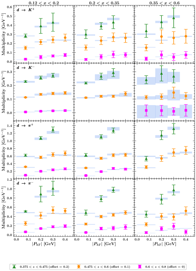
Figure 4: Comparison between data and theoretical predictions for the $\rm HERMES$ multiplicities for the production of charged pions and kaons off a deuteron target for different $x$ and $z$ bins as a function of the transverse momentum $|\bm{P}_{hT}|$ of the final-state hadron. For better visualization, each $z$ bin is shifted by the indicated offset.

We note that for $K^{-}$ production the central column, corresponding to the $0.2<x<0.35$ bin, does not include the magenta points for the highest $0.6<z<0.8$ bin because of the kinematic cut in $z$. Similarly, in all panels there are only three green points (for the lowest $z$ bin) because of the $z$-dependent cut in Eq. (54), which leads to the exclusion of a larger number of $|\bm{q}_{T}|$ bins at lower values of $z$. The theoretical results display larger uncertainties for $K^{-}$ production (second row) because of the combined effect of larger experimental errors and larger uncertainties in the kaon collinear FFs.

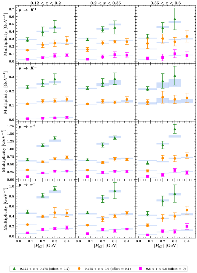
Figure 5: Same conventions and notation as in previous figure but for charged pions and kaons off proton target.

Fig. 5 refers to the same $\rm HERMES$ multiplicities with same conventions and notation as in Fig. 4 but off a proton target. We remark that for $K^{-}$ production the kinematic cuts have a more drastic effect because the magenta points for the $|\bm{P}_{hT}|$ distributions at the largest $z$ bin are excluded for the two largest $x$ bins considered (central and rightmost panels of second row from top).

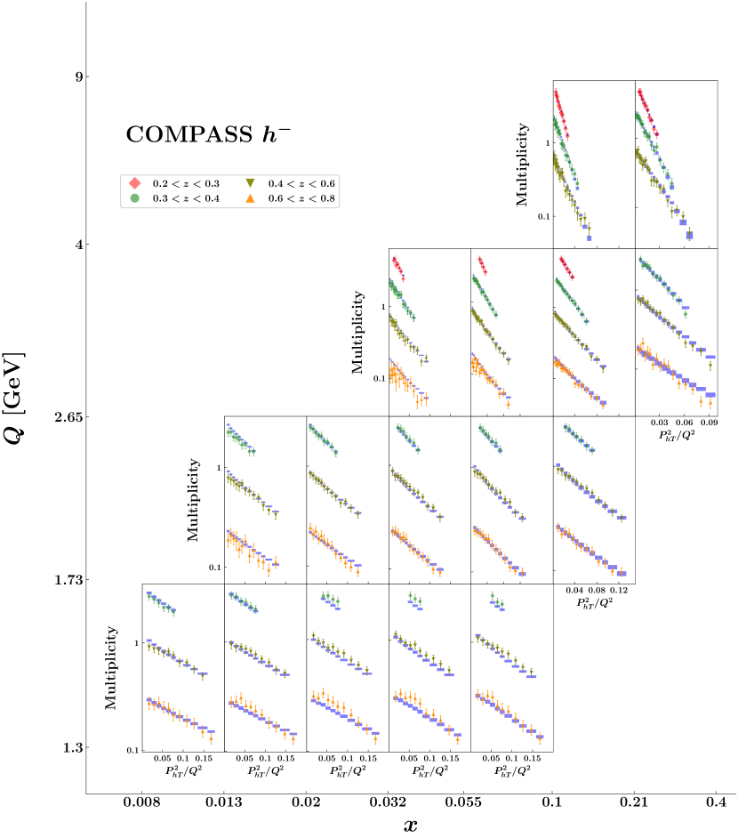
Figure 6: Comparison between data and theoretical predictions for the $\rm COMPASS$ multiplicities for the production of negatively charged hadrons off a deuteron target. For each $Q,x$ bin, the multiplicities are displayed as functions of $\bm{P}_{hT}^{2}/Q^{2}$ for different $z$ bins surviving kinematic cuts, as indicated in the legend.

In Fig. 6, we show the result of our fit for the $\rm COMPASS$ SIDIS multiplicities for the production of unidentified negatively charged hadrons off a deuteron target. For each $Q$ and $x$ bin, each panel displays the multiplicity on a logarithmic scale as a function of $\bm{P}_{hT}^{2}/Q^{2}$. Again, points with different markers and colors correspond to different representative $z$ bins, as indicated in the plot legend. As before, the light-blue rectangles correspond to the 68% CL theoretical results. The results for unidentified negatively charged hadrons $h^{-}$ are obtained by simply adding the results for negatively charged pions and kaons, $h^{-}\sim\pi^{-}+K^{-}$.

We note that the agreement is good for almost all bins, which is reflected in small $\chi^{2}_{0}$ values in Tab. 4. The situation worsens for the lowest $Q$ bin ($1.3<Q<1.73$ GeV), particularly for $x\gtrsim 0.02$. We also remark that for some $Q$ and $x$ bins the theoretical uncertainties for the largest $z$ bin compatible with our kinematic cuts ($0.6<z<0.8$) are significantly larger than for other $z$ bins because of much larger uncertainties in the collinear FFs. Finally, looking at the table of panels from top to bottom, we realize that the lowest $z$-bin distributions (red diamonds) are present only for the largest $Q$ bins, and vice-versa, because of the kinematic cut in Eq. (54)

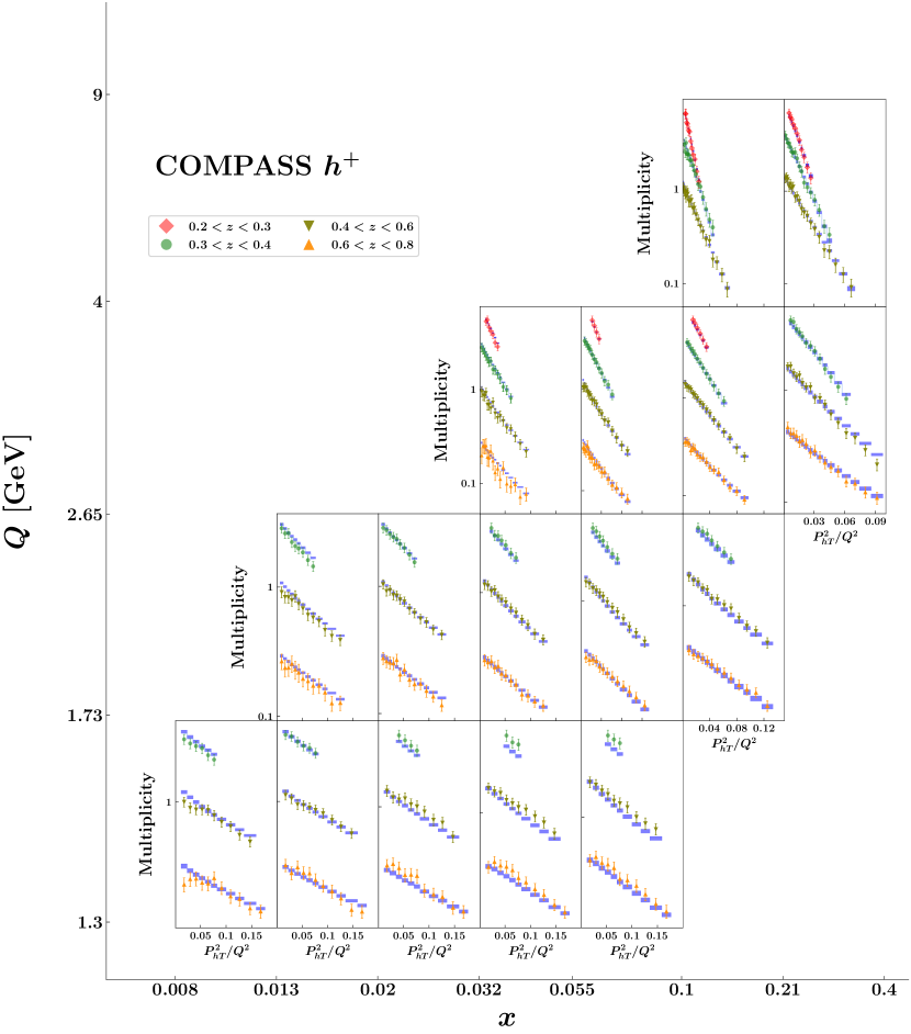
Figure 7: Same conventions and notation as in previous figure but for unidentified positively charged hadrons off deuteron target.

Fig. 7 refers to the same $\rm COMPASS$ multiplicities with same conventions and notation as in Fig. 6 but for unidentified positively charged hadrons $h^{+}$. Again, the light-blue rectangles correspond to the 68% CL theoretical results, and are obtained by adding the results for positively charged pions and kaons, $h^{+}\sim\pi^{+}+K^{+}$. Comments similar to Fig. 6 can be made about the agreement between data and theory.

IV.1.2 Drell-Yan

DY data represents approximately 25% of the full set of analyzed data. From Tab. 4 it is evident that most of low-energy DY data from fixed-target experiments (E605, E288, E772), but also from PHENIX and STAR, can be fitted with low $\chi^{2}$ values, much lower than high-energy DY data from collider experiments like, e.g., those at the LHC. As already pointed out in Ref. Bacchetta:2019sam , this most likely originates from the fact that low-energy DY data are affected by larger errors and collinear PDFs at these kinematics have larger uncertainties.

From Tab. 4, we also note that the quality of our fit for the ATLAS datasets is poor. In particular, the description worsens for the first two low-rapidity bins of both ATLAS 7 TeV and ATLAS 8 TeV datasets, the worst case being at $|y|<1$ for ATLAS 7 TeV. Several effects might be responsible for this result. Since the experimental observable is a normalized cross section, systematic errors cancel in the ratio producing measurements with very small error bars. Fitting these data is very difficult, also because small theoretical effects can give significant contributions to the $\chi^{2}$. Moreover, different implementations of phase-space cuts on the final-state leptons could lead to modifications in both the shape and the normalization of the theoretical observable (see, e.g., Ref. Chen:2022cgv ; Buonocore:2021tke ; Camarda:2021jsw ). We leave this issue for future studies. At variance with Ref. Scimemi:2019cmh , we obtain our results without excluding any extra data points on top of the ones exceeding the maximum value of $|\bm{q}_{T}|/Q$ in Eq. (53).

It is interesting to comment the results of the fit for those datasets that were not included in the previous analysis of Ref. Bacchetta:2019sam (see Sec. III). For E772, we are able to obtain a good description only for data points above the peak of the $\Upsilon$ resonance. For $Q<9$ GeV, the quality of the fit worsens. At variance with Ref. Scimemi:2019cmh , we keep the $Q<9$ GeV bins because there is no evident motivation to exclude them.

The new CMS dataset at $\sqrt{s}=13$ TeV is important because it extends the kinematic coverage considered in Ref. Bacchetta:2019sam . This dataset is very nicely described, even better than the ones at the smaller center-of-mass energies $\sqrt{s}=7,8$ TeV. This is probably due to the fact that the CMS 13 TeV dataset is densely binned in rapidity.

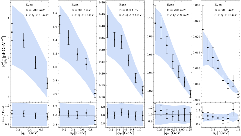
Figure 8: Upper panel: comparison between data and theoretical predictions for the DY cross section differential in $|\bm{q}_{T}|$ for the E288 dataset at $E_{beam}=200$ GeV for different $Q$ bins; uncertainty bands correspond to the 68% CL. Lower panel: ratio between experimental data and theoretical cross section.

In order to visualize the quality of our fit, in Figs. 8-11 we present the comparison between experimental data and theoretical results for a representative selection of the DY dataset. In the upper panels of each plot, we display the cross section differential in $|\bm{q}_{T}|$, while in the lower panels we show the ratio of data to theory. As for the SIDIS case, the light-blue bands are the 68% CL theoretical results.

Fig. 8 displays the DY cross section for the E288 dataset at beam energy $E_{beam}=200$ GeV for different bins in $Q$. For DY fixed-target observables, we calculate the cross section at mean values of $|\bm{q}_{T}|$ (not integrating upon the bin limits). Hence, we display the 68% CL uncertainty as a band rather than a series of rectangles. We remark that the uncertainty band is larger for lower $Q$ bins; this trend is induced by larger correlated uncertainties for smaller invariant masses of the lepton pair.

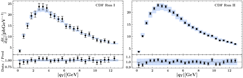
Figure 9: Upper panels: comparison between experimental data and theoretical predictions for the cross section differential in $|\bm{q}_{T}|$ for $Z$ bosons produced in $p\bar{p}$ collisions at the Tevatron from CDF Run I (left panel) and run II (right panel); uncertainty bands correspond to the 68% CL. Lower panel: ratio between experimental data and theoretical results.

In Fig. 9, we compare the theoretical results for the cross section for DY in $p\bar{p}$ collisions at the Tevatron. Black data points in the left panel correspond to the results of Run I of the CDF experiment, while in the right panel the results for Run II are reported. The lower panels show the corresponding ratio of experimental data to theoretical results. The latter are displayed as light-blue rectangles, each one corresponding to the integral of the cross section within the corresponding bin limits. The size of the rectangle is given by the 68% CL. The quality of the fit for CDF data is comparable to the one in Ref. Bacchetta:2019sam .

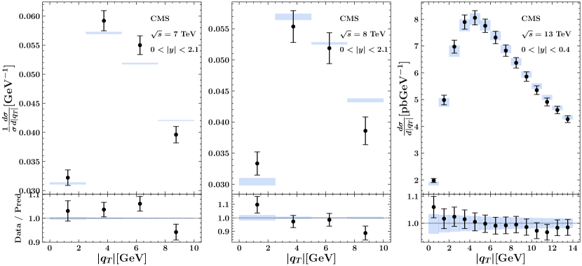
Figure 10: Same as in previous figure but for $Z$ boson production in $pp$ collisions measured by the CMS Collaboration. From left to right: increasing $\sqrt{s}=$ 7, 8, 13 TeV, respectively. For $\sqrt{s}=$ 7, 8 TeV, the results are normalized to the fiducial cross section.

In Fig. 10, we compare the theoretical results for the DY cross section in $pp$ collisions at the LHC. From left to right, the black data points refer to the measurements by the CMS Collaboration at increasing $\sqrt{s}=$ 7, 8, 13 TeV. For $\sqrt{s}=$ 7, 8 TeV, the results are normalized to the fiducial cross section. As in previous figures, the lower panels display the ratio of experimental data to the 68% CL theoretical results. For $\sqrt{s}=$ 7, 8 TeV, the quality of the fit is comparable to that in Ref. Bacchetta:2019sam . For the new dataset at $\sqrt{s}=13$ TeV, the agreement in the displayed rapidity bin is excellent, but remains very good also for higher rapidities.

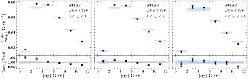
Figure 11: Same as in the left and central panels of previous figure, but for ATLAS kinematics at $\sqrt{s}=7$ TeV. From left to right, results at increasing rapidity.

In Fig. 11, we compare the theoretical results for the DY cross section in $pp$ collisions normalized to the fiducial cross section for the ATLAS data at $\sqrt{s}=7$ TeV. From left to right, we consider three representative bins at increasing rapidity $|y|$. The leftmost one corresponds to the worst described bin in our global fit, with $\chi^{2}/N_{\text{data}}=13.5$. As in previous figures, the lower part of each panel displays the ratio of experimental data to the 68% CL theoretical results. The quality of the fit increases at more forward rapidities (from left to right). The same trend is observed at $\sqrt{s}=8$ TeV, but not for CMS at 13 TeV.

IV.2 TMD distributions

We now discuss the TMD distributions extracted from our baseline fit with N³LL^- accuracy. Tab. 5 displays the list of our 21 fitting parameters with their mean value and standard deviation. The majority of the parameters is well constrained. The only parameter that is compatible with zero is $\gamma_{2}$.

Parameter	Average over replicas
$g_{2}\ [\text{GeV}]$	0.248 $\pm$ 0.008
$N_{1}\ [\text{GeV}^{2}]$	0.316 $\pm$ 0.025
$\alpha_{1}$	1.29 $\pm$ 0.19
$\sigma_{1}$	0.68 $\pm$ 0.13
$\lambda\ [\text{GeV}^{-1}]$	1.82 $\pm$ 0.29
$N_{3}\ [\text{GeV}^{2}]$	0.0055 $\pm$ 0.0006
$\beta_{1}$	10.23 $\pm$ 0.29
$\delta_{1}$	0.0094 $\pm$ 0.0012
$\gamma_{1}$	1.406 $\pm$ 0.084
$\lambda_{F}\ [\text{GeV}^{-2}]$	0.078 $\pm$ 0.011
$N_{3B}\ [\text{GeV}^{2}]$	0.2167 $\pm$ 0.0055
$N_{1B}\ [\text{GeV}^{2}]$	0.134 $\pm$ 0.017
$N_{1C}\ [\text{GeV}^{2}]$	0.0130 $\pm$ 0.0069
$\lambda_{2}\ [\text{GeV}^{-1}]$	0.0215 $\pm$ 0.0058
$\alpha_{2}$	4.27 $\pm$ 0.31
$\alpha_{3}$	4.27 $\pm$ 0.13
$\sigma_{2}$	0.455 $\pm$ 0.050
$\sigma_{3}$	12.71 $\pm$ 0.21
$\beta_{2}$	4.17 $\pm$ 0.13
$\delta_{2}$	0.167 $\pm$ 0.006
$\gamma_{2}$	0.0007 $\pm$ 0.0110

Table 5: Average and standard deviation over the Monte Carlo replicas of the free parameters fitted to the data.

The $\lambda$ parameter measures the relative weight of the first Gaussian and the weighted-Gaussian in the nonperturbative part of the TMD PDF in Eq. (38). The value of this parameter is close to 2, indicating that the contribution of the weighted-Gaussian component is important. In Eq. (38), the parameter $\lambda_{2}$ measures the relative weight of the first Gaussian and the third Gaussian; this parameter is small but not compatible with zero, which means that also this component of the TMD PDF is important to reach a good description of experimental data.

Our parametrization of the nonperturbative part of TMD FFs in Eq. (39) contains just the combination of a Gaussian and a weighted Gaussian: this is sufficient to describe the data in an accurate way.

The $\lambda_{F}$ parameter measures the relative weight of the two components; its value is close to 0.1, indicating that the contribution of the weighted Gaussian is small. Nevertheless, it has non-trivial consequences on the tail of the TMD FF, as we will show below.

The $g_{2}$ parameter is a key ingredient to the extraction of the Collins–Soper kernel, discussed in Sec. IV.2.1. The same parameter was used in the analysis of Ref. Bacchetta:2017gcc . It is interesting to observe that the value obtained in the present global fit is smaller by almost a factor of 4 with respect to Ref. Bacchetta:2017gcc . This may be due to the higher theoretical accuracy of the present analysis and to the role of the very precise high-energy Drell–Yan measurements, which also determine the very small standard deviation of $g_{2}$.

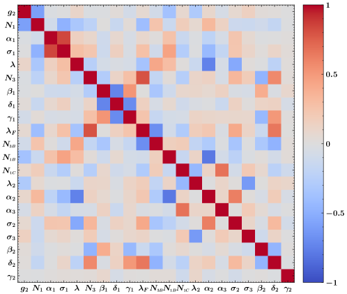
Figure 12: Graphical representation of the correlation matrix for the fitted parameters.

In Fig. 12, we show a graphical representation of the correlations among the 21 fitting parameters. Using the color code indicated in the legend, it is easy to realize that the nondiagonal elements are very small except for some (anti–)correlation among the $\beta_{1}$, $\delta_{1}$ and $\gamma_{1}$ parameters that control the $z$–dependent width of the Gaussians in the TMD FF (see Eqs. (39), (41)). The overall absence of large correlations suggests that the model parametrization of the non perturbative parts of TMDs is appropriate.

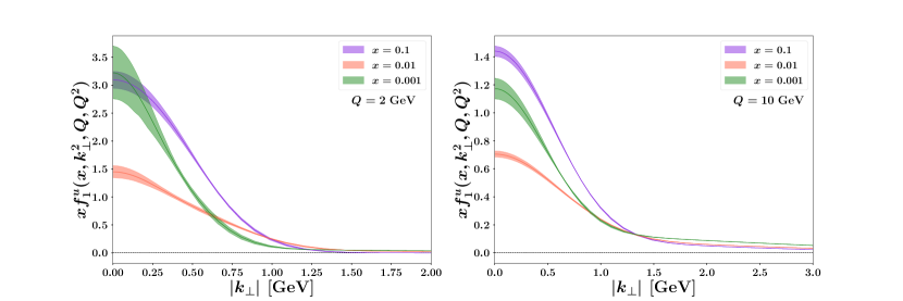
Figure 13: The TMD PDF of the up quark in a proton at $\mu=\sqrt{\zeta}=Q=2$ GeV (left panel) and 10 GeV (right panel) as a function of the partonic transverse momentum $|\bm{k}_{\perp}|$ for $x$ = 0.001, 0.01 and 0.1. The uncertainty bands represent the 68% CL.

In Fig. 13, we show the unpolarized TMD PDF for the up quark in the proton at $\mu=\sqrt{\zeta}=Q=2$ GeV (left panel) and 10 GeV (right panel) as a function of the quark transverse momentum $|\bm{k}_{\perp}|$ for three different values of $x$, namely $x$ = 0.001, 0.01, and 0.1. The bands correspond to the 68$\%$ CL.

The TMD seems to be wider at intermediate $x=0.01$, but has also a high tail at $x=0.001$. As already mentioned, a significant role is played by the weighted Gaussian and by the second Gaussian in Eq. (38). This may be a sign of the presence of contributions from different quark flavors and/or from different spin configurations (see Sec. II.3).

It is worth noticing that in both left and right panels the TMD PDF at $x=0.001$ shows the largest error band, particularly at low $|\bm{k}_{\perp}|$. This is due to the lack of experimental points in that kinematic region (see Fig. 3). Future data from the Electron-Ion Collider (EIC) are expected to play an important role in getting a better description of the TMD PDFs at low $x$ AbdulKhalek:2021gbh ; AbdulKhalek:2022erw .

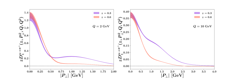
Figure 14: The TMD FF for an up quark fragmenting into a $\pi^{+}$ at $\mu=\sqrt{\zeta}=Q=2$ GeV (left panel) and 10 GeV (right panel) as a function of the hadron transverse momentum $|\bm{P}_{\perp}|$ for $z$ = 0.3 and 0.6. The uncertainty bands represent the 68$\%$ CL.

In Fig. 14, we show the TMD FF for the up quark fragmenting into a $\pi^{+}$ at $\mu=\sqrt{\zeta}=Q=2$ GeV (left panel) and 10 GeV (right panel) as a function of the pion transverse momentum $|\bm{P}_{\perp}|$ (with respect to the fragmenting quark axis) for two different values of $z=$ 0.3 and 0.6. As in the previous figure, the uncertainty bands correspond to the 68$\%$ CL. In both left and right panels, an additional structure clearly emerges at intermediate $P_{\perp}$, especially at $z=0.3$, which is induced by the weighted Gaussian in Eq. (39). Further investigations on this topic are needed, and data from electron-positron annihilations would be valuable to better explore these features.

We stress that the error bands displayed in Figs. 13-14 reflect the uncertainty on the fitted parameters (see Eqs. (38)-(39)) that are determined by taking into account the uncertainty on the collinear PDFs and FFs as discussed in Sec. III.3. However, since the fits are performed using the central set of the collinear distributions, all TMD replicas have the same integral in $\bm{k}_{\perp}$ (i.e., their values at $\bm{b}_{T}=0$ are the same). As a consequence, the plots in Figs. 13-14 only partially account for the error of the collinear distributions.

IV.2.1 Collins–Soper kernel

It is interesting to study the Collins–Soper kernel Collins:1981uk ; Collins:2011zzd that drives the evolution of TMDs in terms of the rapidity scale $\zeta$. Recent discussions of this crucial component of the TMD formalism have been presented in Refs. Vladimirov:2020umg ; Martinez:2022gsz and estimates based on lattice QCD have been proposed in Refs. Schlemmer:2021aij ; Shanahan:2021tst ; LPC:2022ibr .

The Collins–Soper kernel, as written in Eq. (36), is composed of two parts. The first part can be calculated perturbatively at N^kLL accuracy, and is computed at $b_{\ast}$:

$$K(b_{*}(|\mathbf{b}_{T}|),\mu)=\sum_{n=0}^{k-1}\left(\frac{\alpha_{s}(\mu_{b_{*}})}{4\pi}\right)^{n+1}K^{(n,0)}-\sum_{n=0}^{k}\gamma_{K}^{(n)}\int_{\mu_{b_{*}}}^{\mu}\frac{d\mu^{\prime}}{\mu^{\prime}}\left(\frac{\alpha_{s}(\mu^{\prime})}{4\pi}\right)^{n+1}\,,$$ (58)

where $K^{(n,0)}$ and $\gamma_{K}^{(n)}$ are coefficients of the perturbative expansion (see, e.g., Ref. Collins:2017oxh ). Note that the integral on the r.h.s. is directly computed by means of numerical integration, thus providing a fully resummed result. The second part, denoted as $g_{K}$, cannot be computed in perturbation theory and is one of the results of our fit. Only the full Collins–Soper kernel can be compared with other works.

In Fig. 15, we show the Collins–Soper kernel as a function of $|\bm{b}_{T}|$ by conventionally keeping the scale $\mu$ fixed at 2 GeV, for our present analysis (MAPTMD22, green band) and for four other analyses in the literature Bacchetta:2017gcc ; Scimemi:2017etj ; Bacchetta:2019sam ; Scimemi:2019cmh . The solid lines at low $|\bm{b}_{T}|$ follow the perturbative result. For MAPTMD22, PV19 Bacchetta:2019sam and PV17 Bacchetta:2017gcc , they correspond to setting $b_{\mathrm{min}}=0$ for sake of comparison with the other SV19 Scimemi:2019cmh , SV17 Scimemi:2017etj results. The slight differences between the curves are due to the different logarithmic accuracies of the perturbative calculations: the PV17 analysis was performed at NLL, the SV17 analysis at N²LL, the PV19, SV19 and MAPTMD22 at N³LL. The size of the bands around the solid lines corresponds to one standard deviation of the parameter $g_{2}$ around its best-fit value. The $b_{\ast}$ prescription modifies the curves starting from $|\bm{b}_{T}|\approx 1$ GeV^-1. The behavior at high $|\bm{b}_{T}|$ is driven by $g_{K}$ and is different for the various analyses.

The dashed curves show the effect of using our prescription $b_{\mathrm{min}}=2e^{-\gamma_{E}}/\mu\approx 1.123/\mu$ in MAPTMD22, PV19 and PV17. This implies that at low $|\bm{b}_{T}|$ the Collins–Soper kernel saturates to a finite value, as indicated by the dashed lines. As the scale increases, this modification occurs at lower and lower values of $|\bm{b}_{T}|$ and becomes less relevant.

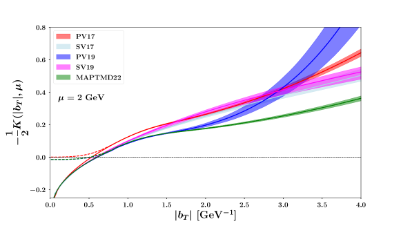
Figure 15: The Collins–Soper kernel as a function of $|\bm{b}_{T}|$ at a scale $\mu=2$ GeV from the present analysis (MAPTMD22), compared with the PV17 Bacchetta:2017gcc , SV17 Scimemi:2017etj , PV19 Bacchetta:2019sam , and SV19 Scimemi:2019cmh analyses. For the MAPTMD22, PV17, and PV19 curves, the uncertainty bands represent the 68% CL. The corresponding dashed lines show the effect of including the $b_{\text{min}}$-prescription (see text).

IV.2.2 Average squared transverse momenta

The average squared transverse momenta $\langle\bm{k}_{\perp}^{2}\rangle(x,Q)$, $\langle\bm{P}_{\perp}^{2}\rangle(z,Q)$ are calculated with the Bessel weighting technique suggested in Refs. Boer:2011xd ; Boer:2014bya .

In the case of the TMD PDF for a quark $q$ in the proton at $\mu=\sqrt{\zeta}=Q$, one has Boer:2011xd ; Boer:2014bya :

$$\langle\bm{k}_{\perp}^{2}\rangle^{q}(x,Q) =\frac{\int d^{2}\bm{k}_{\perp}\,\bm{k}_{\perp}^{2}\,f_{1}^{q}(x,\bm{k}_{\perp}^{2},Q,Q^{2})}{\int d^{2}\bm{k}_{\perp}\,f_{1}^{q}(x,\bm{k}_{\perp}^{2},Q,Q^{2})}=\frac{2M^{2}\,\hat{f}_{1}^{q\,(1)}(x,|\bm{b}_{T}|,Q,Q^{2})}{\hat{f}_{1}^{q}(x,|\bm{b}_{T}|,Q,Q^{2})}\bigg{|}_{|\bm{b}_{T}|=0}\,,$$ (59)

where the Fourier transform $\hat{f}_{1}^{q}$ of the TMD PDF has been defined in Eq. (5) and the first Bessel moment of the TMD PDF $\hat{f}_{1}^{q\,(1)}$ is defined as Boer:2011xd :

$$\hat{f}_{1}^{q\,(1)}(x,|\bm{b}_{T}|,Q,Q^{2})=\frac{2\pi}{M^{2}}\,\int_{0}^{+\infty}d|\bm{k}_{\perp}|\,\frac{\bm{k}_{\perp}^{2}}{|\bm{b}_{T}|}\,J_{1}\big{(}|\bm{k}_{\perp}||\bm{b}_{T}|\big{)}\,f_{1}^{q}(x,\bm{k}_{\perp}^{2},Q,Q^{2})=-\frac{2}{M^{2}}\frac{\partial}{\partial\bm{b}_{T}^{2}}\hat{f}_{1}^{q\,}(x,|\bm{b}_{T}|,Q,Q^{2})\,.$$ (60)

In order to obtain meaningful values for the average squared transverse momenta, i.e., finite, positive, and not dominated by the perturbative tails of the TMDs, we shift the value of $|\bm{b}_{T}|$ from 0 to a value well inside the nonperturbative region Boer:2014bya . In this way the Bessel functions $J_{0,1}$ tame the power-law behavior of the TMD at large transverse momentum. The choice of the specific value for $|\bm{b}_{T}|$ is of course arbitrary and has a significant effect on the associated numerical values. We choose $|\bm{b}_{T}|=1.5\,b_{\text{max}}$ that guarantees that the average squared transverse momenta are positive across the $x$, $Q$ values considered in the fit. Accordingly, Eq. (60) becomes:

$$\langle\bm{k}_{\perp}^{2}\rangle^{q}_{r}(x,Q)=\frac{2M^{2}\,\hat{f}_{1}^{q\,(1)}(x,|\bm{b}_{T}|,Q,Q^{2})}{\hat{f}_{1}^{q}(x,|\bm{b}_{T}|,Q,Q^{2})}\bigg{|}_{|\bm{b}_{T}|=1.5\,b_{\text{max}}}\,,$$ (61)

where the subscript $r$ stands for regularized. We have checked that the results are consistent when choosing either the integral or differential expressions in Eq. (60).

The same arguments apply to the regularized average squared transverse momentum produced during the hadronization of the quark $q$ into the final state hadron $h$ Boer:2011xd ; Boer:2014bya ; Bacchetta:2019qkv :

$$\langle\bm{P}_{\perp}^{2}\rangle^{q\to h}_{r}(z,Q) =\frac{2\,z^{2}\,M_{h}^{2}\,\hat{D}_{1}^{q\to h\,(1)}(z,|\bm{b}_{T}|,Q,Q^{2})}{\hat{D}_{1}^{q\to h}(z,|\bm{b}_{T}|,Q,Q^{2})}\bigg{|}_{|\bm{b}_{T}|=1.5\,b_{\text{max}}}\,,$$ (62)

where the Fourier transform $\hat{D}_{1}^{q\to h}$ of the TMD FF is defined in Eq. (26) and the first Bessel moment of the TMD FF $\hat{D}_{1}^{q\to h\,(1)}$ is defined as Bacchetta:2019qkv :

$$\begin{split}\hat{D}_{1}^{q\to h\,(1)}(z,|\bm{b}_{T}|,Q,Q^{2})&=\frac{2\pi}{M_{h}^{2}}\,\int_{0}^{+\infty}\frac{d|\bm{P}_{\perp}|}{z}\,\frac{|\bm{P}_{\perp}|}{z}\,\frac{|\bm{P}_{\perp}|}{z|\bm{b}_{T}|}\,J_{1}\big{(}|\bm{b}_{T}||\bm{P}_{\perp}|/z\big{)}\,D_{1}^{q\to h}(z,\bm{P}_{\perp}^{2},Q,Q^{2})\\ &=-\frac{2}{M_{h}^{2}}\frac{\partial}{\partial\bm{b}_{T}^{2}}\hat{D}_{1}^{q\to h}(z,|\bm{b}_{T}|,Q,Q^{2})\,.\end{split}$$ (63)

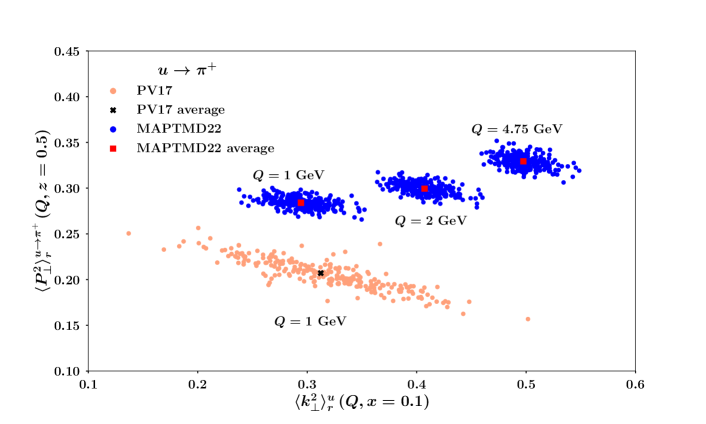
Figure 16: Scatter plot of average squared transverse momenta for the TMD PDF of the up quark at $x=0.1$ and for the TMD FF of the $u\to\pi^{+}$ fragmentation at $z=0.5$. Orange circles for the PV17 analysis Bacchetta:2017gcc at NLL at $Q=1$ GeV; the black cross represents the average. Blue circles for this analysis (MAPTMD22) at N³LL^- and at $Q=$ 1, 2, 4.75 GeV; the red squares represent the average values for each considered $Q$ value.

In Fig. 16, we show the scatter plot of $\langle\bm{k}_{\perp}^{2}\rangle^{u}_{r}$ (up quark contribution) at $x=0.1$ vs. $\langle\bm{P}_{\perp}^{2}\rangle_{r}^{u\to\pi^{+}}$ (“favored” fragmentation) at $z=0.5$. The blue circles (denoted by MAPTMD22) correspond to the single replicas while the red square is the average over all replicas for the N³LL^- analysis. Three different values of $Q=$ 1, 2, 4.75 GeV are included to show the evolution of the average transverse momenta with the scale. The orange circles indicate the PV17 replicas Bacchetta:2017gcc at NLL and $Q=1$ GeV with the black cross being the average. No regularization is needed for the values extracted in the PV17 analysis, since the involved TMDs at $Q=1$ reduce entirely to their nonperturbative components. By comparing MAPTMD22 at $Q=1$ GeV to PV17, we observe that the former produces much less anti-correlation between $\langle\bm{k}_{\perp}^{2}\rangle$ and $\langle\bm{P}_{\perp}^{2}\rangle$ than the latter, probably because of the inclusion of very precise DY data.

IV.3 Variations on the fit configurations

In this subsection we discuss the results obtained by modifying some of the baseline settings. In Sects. IV.3.1 and IV.3.2 we present fits at NNLL and NLL accuracy, respectively, comparing them to the baseline N³LL^-. Finally, in Sec. IV.3.3 we study the impact of adopting different cuts in $|\bm{q}_{T}|$ on the SIDIS dataset.

	N3LL-		NNLL		NLL
Data set	$N_{\rm dat}$	$\langle\chi^{2}\rangle\pm\delta\langle\chi^{2}\rangle$	$N_{\rm dat}$	$\langle\chi^{2}\rangle\pm\delta\langle\chi^{2}\rangle$	$N_{\rm dat}$	$\langle\chi^{2}\rangle\pm\delta\langle\chi^{2}\rangle$
ATLAS	72	5.01 $\pm$ 0.26	/	/	/	/
PHENIX 200	2	3.26 $\pm$ 0.31	2	0.81 $\pm$ 0.11	/	/
STAR 510	7	1.16 $\pm$ 0.04	7	0.99 $\pm$ 0.03	/	/
Other sets	170	0.83 $\pm$ 0.01	170	2.37 $\pm$ 0.11	/	/
DY collider	251	2.06 $\pm$ 0.07	179	2.3 $\pm$ 0.1	/	/
E772	53	2.48 $\pm$ 0.12	53	2.05 $\pm$ 0.22	/	/
Other sets	180	0.87 $\pm$ 0.04	180	0.71 $\pm$ 0.04	180	0.81 $\pm$ 0.04
DY fixed-target	233	1.24 $\pm$ 0.04	233	1.01 $\pm$ 0.05	180	0.81 $\pm$ 0.04
HERMES	344	0.71 $\pm$ 0.04	344	1.1 $\pm$ 0.06	344	0.51 $\pm$ 0.02
COMPASS	1203	0.95 $\pm$ 0.02	1203	0.6 $\pm$ 0.06	1203	0.41 $\pm$ 0.01
SIDIS	1547	0.89 $\pm$ 0.02	1547	0.71 $\pm$ 0.05	1547	0.43 $\pm$ 0.01
Total	2031	1.08 $\pm$ 0.01	1959	0.89 $\pm$ 0.01	1727	0.47 $\pm$ 0.01

Table 6: Comparison of $\chi^{2}$ values normalised to the number of data points $N_{\text{dat}}$ for fits at different perturbative accuracies. The $\langle\chi^{2}\rangle$ and $\delta\langle\chi^{2}\rangle$ are the average and standard deviation of the $\chi^{2}$ values of all replicas.

IV.3.1 Global fit at NNLL

The baseline fit presented in the previous section is performed at N³LL^- (see Tab. 1). As already emphasized in Ref. Bacchetta:2019sam , the inclusion of perturbative corrections up to N³LL is crucial to achieve an optimal description of some of the most recent experimental measurements, such as those by the LHC. However, it might be useful to extract unpolarized TMDs at lower perturbative orders. One of the reasons is that such sets can be used in global analyses of polarized TMDs where it is not possible to reach the same level of accuracy.

This is the case of the Sivers TMDs where the computation of the polarized cross section for the Sivers effect presently cannot go beyond the NNLL level Bacchetta:2020gko ; Echevarria:2020hpy ; Bury:2021sue , hence demanding unpolarised TMDs at the same level of accuracy.

To this aim, we perform a new global fit at NNLL. However, when lowering the perturbative accuracy, it is possible to obtain acceptably good fits only by excluding those datasets whose precision requires the highest theoretical accuracy. Specifically, we found that only by removing the ATLAS dataset we were able to achieve an acceptable global description at NNLL accuracy. As a matter of fact, in Tab. 6 the value of $\chi^{2}$ in this configuration, namely for fixed-target DY and SIDIS, is lower than at N³LL^- where ATLAS data is included.

Because of the difference in the perturbative accuracy as well as in the dataset, we do not expect to get compatible values for the best fit parameters between the NNLL and N³LL^- fits. For instance, we obtain $\lambda=12\pm 10$ GeV^-1 and $\lambda_{F}=340\pm 280$ GeV^-2 at NNLL, to be compared to $\lambda=1.8\pm 0.3$ GeV^-1 and $\lambda_{F}=0.08\pm 0.01$ GeV^-2 at N³LL^-.

The $\lambda$ and $\lambda_{F}$ parameters control the relative weight of the weighted Gaussian in the non perturbative part of the TMD PDF and FF, respectively, and control the size of the DY and SIDIS spectrum at middle to large values of $|\bm{q}_{T}|$. The large values obtained in the NNLL imply that the weighted Gaussian dominates for both TMD PDF and FF parametrizations. This behavior may be partially induced by the lack of perturbative corrections of the NNLL fit with respect to the N³LL^- one, which are compensated by nonperturbative effects.

IV.3.2 Global fit at NLL

We performed also a global analysis at NLL accuracy. Similarly to the NNLL fit discussed above, it might be useful to have also a global fit at NLL accuracy for contexts where it is not possible to reach the highest accuracy. However, in order to obtain acceptable $\chi^{2}$ values at this order, we had to exclude all collider DY data and the E772 fixed-target DY dataset. Thus, we reduced the dataset to the SIDIS data and the remaining fixed-target DY data, i.e., E605 and E288.

We point out that in our approach the integral of the $W$-term at NLL is equal by construction to the SIDIS $\bm{q}_{T}$-integrated collinear cross section. As a consequence, the value of the prefactor $\omega$ in Eq. (52) is automatically equal to 1. Moreover, for this fit we consistently used MMHT2014 at LO for the collinear PDFs and we used DSS at NLO for collinear FFs. As shown in Tab. 1, at NLL both collinear PDFs and FFs should be evaluated at LO, but we choose FFs at NLO because no recent extractions at LO are currently available.

As can be seen in Tab. 6, we obtain low $\chi^{2}$ values for all included datasets. It is interesting to compare this result with that of the PV17 analysis Bacchetta:2017gcc . In that work, the normalization of $\rm COMPASS$ data was fixed by the first bin in $\bm{P}_{hT}^{2}$. Here we demonstrate that we can obtain an excellent description of the most recent $\rm COMPASS$ data without any adjustment of the normalization.

IV.3.3 Cut in $|q_{T}|/Q$

A crucial ingredient of any phenomenological analysis of TMDs is the introduction of the kinematic cut $|\bm{q}_{T}|/Q\ll 1$ on the dataset to ensure that TMD factorization is valid. Our default choices are discussed in Sec. III. It is interesting to study how the global quality of our fit changes upon variations of this cut in order to get quantitative information on the range of validity of TMD factorization.

To this purpose, we changed the parameters $c_{1}$, $c_{2}$, and $c_{3}$ in Eq. (54) devised for the SIDIS data, while keeping the constraint $|\bm{q}_{T}|/Q<0.2$ for the DY data. We refer the reader to Ref. Bacchetta:2019sam for an analogous study of the effect of the $|\bm{q}_{T}|/Q$ cut on the DY data.

We consider five different configurations for the cut on SIDIS data:

• A first and most conservative cut is performed by fixing the z-independent upper value $|\bm{q}_{T}|/Q<0.4$ which can be obtained by setting $c_{1}=c_{2}=0.4$ and $c_{3}=0$ in Eq. (54);

• A second cut by setting $c_{1}=0.15$, $c_{2}=0.4$ and $c_{3}=0.2$ in Eq. (54);

• The cut of our baseline fit with $c_{1}=0.2$, $c_{2}=0.5$ and $c_{3}=0.3$;

• A fourth cut with $c_{1}=0.2$, $c_{2}=0.6$ and $c_{3}=0.4$ but without imposing $|\bm{q}_{T}|<Q$ (i.e. removing the outermost “min” in Eq. (54));

• A fifth cut inspired by the PV17 analysis Bacchetta:2017gcc , namely the same as in the previous case but with $c_{1}=0.2$, $c_{2}=0.7$ and $c_{3}=0.5$; this is the least conservative choice.

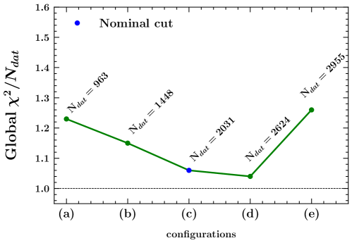
Figure 17: Global $\chi^{2}/N_{\text{dat}}$ for different configurations of the kinematic cut on SIDIS data sets (see text). The blue point corresponds to the reference cut used in the present baseline fit.

In Fig. 17, we show how the global $\chi^{2}/N_{\text{dat}}$ changes when considering the five configurations described above. By observing that more conservative choices do not necessarily correspond to better $\chi^{2}$ values, we conclude that the TMD formalism is able to describe SIDIS data that fails to fulfil the formal requirement $|\bm{q}_{T}|/Q\ll 1$. In this respect, we notice that the global $\chi^{2}/N_{\text{dat}}$ of cut (d) is smaller than the baseline fit, despite including a larger amount of data, some of which at $|\bm{q}_{T}|\gtrsim Q$, i.e., well outside the region where TMD factorization is valid.

In Fig. 18, we better illustrate the situation by showing the comparison between $\rm COMPASS$ data and theoretical predictions from our baseline fit for the SIDIS multiplicity for positively charged hadrons as a function of $|\bm{P}_{hT}|/Q$ in the bin $1.3<Q<1.73$ GeV, $0.02<x<0.032$, $0.3<z<0.4$. The upper panel of the plot displays the multiplicity while the lower panel shows the ratio of experimental data to the theoretical predictions. The solid circles indicate data points included in the fit while empty squares refer to those that do not survive the cut. Remarkably, the agreement remains very good up to $|\bm{P}_{hT}|/Q\simeq 0.5$, well beyond the largest $|\bm{P}_{hT}|$ allowed by the cut. We also stress that this behavior is not specific of the considered bin but is a general feature also of other bins, as well as of the $\rm HERMES$ dataset.

In conclusion, from our analysis it emerges that the validity of the TMD formalism in the kinematic region covered by $\rm COMPASS$ and $\rm HERMES$ seems to extend well beyond the customary cut $|\bm{q}_{T}|/Q\ll 1$.

This evidence justifies in a quantitative way our choice for the cut $|\bm{q}_{T}|/Q$ in Eq. (54) for the baseline fit, and explains why we obtain values of $\chi^{2}/N_{\text{dat}}$ close to one also with less conservative cuts. Moreover, it suggests that the applicability of TMD factorization in SIDIS might be defined in terms of $|\bm{P}_{hT}|$ rather than $|\bm{q}_{T}|$, calling for more extensive studies in this direction.

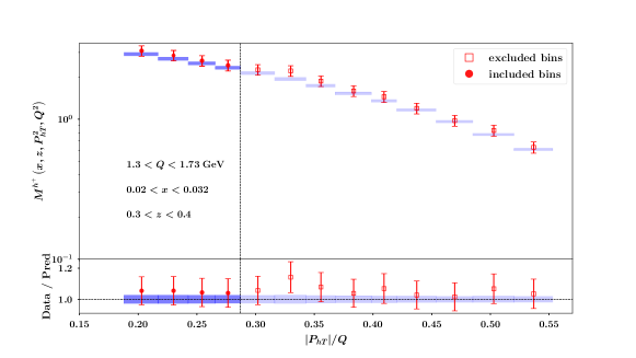
Figure 18: Comparison between $\rm COMPASS$ multiplicities and theoretical results for the SIDIS production of unidentified positively charged hadrons off a deuteron target at $1.3<Q<1.73$ GeV, $0.02<x<0.032$ and $0.3<z<0.4$ as a function of $|\bm{P}_{hT}|/Q$. Upper panel: light-blue rectangles for baseline fit at 68% CL, empty squares for data points not included in the baseline fit. Lower panel: ratio between experimental data and theoretical results.

V Conclusions and outlook

In this article, we presented an extraction of unpolarized Transverse-Momentum Dependent Parton Distribution Functions and Fragmentation Functions (TMD PDFs and TMD FFs, respectively), which we refer to as MAPTMD22.

We analyzed 2031 data points collected by several experiments: 251 data points from Drell–Yan (DY) production measured at Tevatron, LHC and RHIC, 233 points from fixed-target DY (see Tab. 2) and 1547 data points from Semi-Inclusive Deep Inelastic Scattering (SIDIS) measured by the HERMES and COMPASS collaborations (see Tab. 3).

Our description of the experimental observables is based on TMD factorization at a perturbative accuracy defined as N³LL^-, in the sense that we use TMD evolution at the N³LL level, hard factor and matching coefficients at order $\alpha^{2}_{s}$, collinear PDFs at NNLO, and collinear FFs at NLO (see Tab. 1).

We constructed the full TMDs by combining the perturbative components, regularized by means of the $b_{\ast}$ prescription defined in Eq. (33), and nonperturbative parts described as a sum of Gaussians and weighted Gaussians (see Eqs. (38) and (39)). We used 21 free parameters: 11 related to the TMD PDF, 9 for the TMD FF, and one for the Collins–Soper kernel driving the TMD evolution. We assumed these parameters to be the same for all quark flavors.

The TMD formalism is applicable only if observed transverse momenta are much smaller than the hard scale $Q$ of the considered process. The details of our data selection are explained in Sec. III. In the DY case, for the final lepton pair transverse momentum $\bm{q}_{T}$ we adopted a simple criterion, $|\bm{q}_{T}|<0.2\,Q$, which is common to other works in the literature. In the SIDIS case, our selection criterion is more restrictive than the one made in Ref. Bacchetta:2017gcc , but less restrictive than the one made in Ref. Scimemi:2019cmh . For SIDIS data, where the detected hadron momentum is $\bm{P}_{hT}\approx-z\bm{q}_{T}$, our cut includes many data points with $|\bm{P}_{hT}|\ll Q$ but also with $0.2\,Q<|\bm{q}_{T}|<Q$.

We also tested the quality of our fit by exploring other criteria for the $|\bm{q}_{T}|/Q$ cut. Surprisingly, we find that fits of quality comparable to the baseline result can be obtained with less conservative cuts such that $|\bm{q}_{T}|\gtrsim Q$ for several data points. We believe that the definition of the range of applicability of the TMD factorization formula deserves further studies.

We found it difficult to reproduce the normalization of SIDIS data measured in fixed-target experiments at moderate to low scales. The formalism works well at NLL order, but severely underestimates the data at the N²LL order and above. The reason can be traced back to the fact that the integral upon transverse momentum of the TMD cross section coincides with the known collinear result only at NLL, while it misses other contributions at higher orders. A rigorous solution of the problem would imply the calculation of all these contributions (including the so-called $Y$-term in the language of Ref. Collins:2011zzd ), which are currently not under control, and are beyond the scope of this work. We decided to modify our predictions by including pre-computed normalization factors that are independent of the fit, and that are identified by comparing the integral upon transverse momenta of the TMD formula to the corresponding collinear calculation, as explained in Sec. II.4.

The fit is performed with the bootstrap method, leading to an ensemble of 250 replicas. We reach a very good overall agreement with data, with $\chi^{2}/N_{\rm dat}=1.06$ for the central replica (defined in Sec. IV.1). The description of all individual datasets is satisfactory, except for a few cases, in particular for the ATLAS data (see Tab. 4 and Fig. 11). The discrepancy with the ATLAS data may be due to corrections not fully included in our analysis (see, e.g., Ref. Chen:2022cgv ) which, in spite of being small, can have a large impact in the comparison with very high precision data.

The resulting TMDs are shown in Figs. 13 and 14. It is interesting to note that they deviate from a simple Gaussian shape (especially for the FFs) and the TMD shape changes in a nontrivial way as a function of $x$ or $z$. Tables with grids of the obtained TMDs will be made publicly available at the NangaParbat website and the TMDlib website Abdulov:2021ivr .

The availability of TMD analyses at increasing precision will be essential in guiding detector design and feasibility studies for the future Electron Ion Collider, and will also have a strong impact on precision measurements of observables particularly sensitive to the hadron structure, such as $W$ mass measurements at hadron colliders (see, e.g., Refs.Bacchetta:2018lna ; Bozzi:2019vnl ; CDF:2022hxs ).

Our work can be extended by improving the perturbative accuracy of the analysis (see, e.g., Refs. Camarda:2021ict ; Chen:2022cgv ), including theoretical uncertainties in terms of suitable scale variations (along the lines of Ref. Bertone:2022sso ), improving the treatment of correlated uncertainties, and investigating possible flavor dependence of TMDs Signori:2013mda ; Bury:2022czx .

Appendix A Explicit expression of $C$ coefficients at order $\alpha_{s}$

For completeness, in this Appendix we report the explicit expression of the coefficients mentioned Sec. II.4. The $C^{ab}_{\mathrm{TMD}}$ coefficients of Eq. (45) are given by:

$$\begin{split}C_{\rm TMD}^{qq}(x,z)&=2C_{F}\biggl{(}-8\delta(1-x)\delta(1-z)+\delta(1-x)\Bigl{[}2L_{2}(z)+(1-z)\Bigr{]}+\delta(1-z)(1-x)\biggr{)},\end{split}$$ (64)

$$C_{\rm TMD}^{gq}(x,z) =2C_{F}\biggl{(}P_{gq}(z)\delta(1-x)\ln\left(z(1-z)\right)+z\delta(1-x)\biggr{)},$$ (65)

$$C_{\rm TMD}^{qg}(x,z) =2T_{F}\biggl{(}\delta(1-z)2x(1-x)\biggr{)}.$$ (66)

They correspond to the combination of the matching coefficients $C^{ab}$ included in the TMD PDFs and FFs in Sec. II.3. The following $C^{ab}_{\mathrm{nomix}}$ coefficients are the ones included in the computation of the SIDIS normalization factors of Eq. (50):

$$\begin{split}C_{\rm nomix}^{qq}(x,z;Q,\mu)&=C_{\rm TMD}^{qq}(x,z)+2C_{F}\Biggl{[}\delta(1-x)\Biggl{(}P_{qq}(z)\ln\frac{Q^{2}}{\mu^{2}}+L_{1}(z)-L_{2}(z)\Biggr{)}\\ &\quad+\delta(1-z)\Biggl{(}P_{qq}(x)\ln\frac{Q^{2}}{\mu^{2}}+L_{1}(x)-L_{2}(x)\Biggr{)}\Biggr{]},\end{split}$$ (67)

$$C_{\rm nomix}^{gq}(x,z;Q,\mu) =C_{\rm TMD}^{gq}(x,z)+2C_{F}\delta(1-x)P_{gq}(z)\ln\frac{Q^{2}}{\mu^{2}},$$ (68)

$$C_{\rm nomix}^{qg}(x,z;Q,\mu) =C_{\rm TMD}^{qg}(x,z)+2T_{F}\delta(1-z)P_{qg}(x)\ln\left(\frac{Q^{2}}{\mu^{2}}\frac{1-x}{x}\right).$$ (69)

Finally, the missing contributions to Eq. (49), $C^{ab}_{\mathrm{mixed}}$, are given by:

$$\begin{split}C_{\rm mixed}^{qq}(x,z;Q,\mu)&=2C_{F}\Biggl{[}2\frac{1}{(1-x)_{+}}\frac{1}{(1-z)_{+}}-\frac{1+z}{(1-x)_{+}}-\frac{1+x}{(1-z)_{+}}+2(1+xz)\Biggr{]},\end{split}$$ (70)

$$C_{\rm mixed}^{gq}(x,z;Q,\mu) =2C_{F}\Biggl{[}P_{gq}(z)\frac{1}{(1-x)_{+}}+2(1+x-xz)-\frac{1+x}{z}\Biggr{]},$$ (71)

$$C_{\rm mixed}^{qg}(x,z;Q,\mu) =2T_{F}P_{qg}(x)\left[\frac{1}{(1-z)_{+}}+\frac{1}{z}-2\right].$$ (72)

In the above expressions $\mu$ denotes the factorization scale for PDFs or FFs, while $L_{1,2}$ are abbreviations for the following logarithmic functions:

$$L_{1}(\xi)\equiv\left(1+\xi^{2}\right)\left(\frac{\ln(1-\xi)}{1-\xi}\right)_{+},\qquad L_{2}(\xi)\equiv\frac{1+\xi^{2}}{1-\xi}\ln\xi.$$ (73)

- (1) T. C. Rogers, An overview of transverse-momentum–dependent factorization and evolution, Eur. Phys. J. A 52 (2016) 153, [1509.04766].
- (2) M. Diehl, Introduction to GPDs and TMDs, Eur. Phys. J. A 52 (2016) 149, [1512.01328].
- (3) R. Angeles-Martinez et al., Transverse Momentum Dependent (TMD) parton distribution functions: status and prospects, Acta Phys. Polon. B 46 (2015) 2501–2534, [1507.05267].
- (4) I. Scimemi, A short review on recent developments in TMD factorization and implementation, Adv. High Energy Phys. 2019 (2019) 3142510, [1901.08398].
- (5) A. Bacchetta, F. Delcarro, C. Pisano, M. Radici and A. Signori, Extraction of partonic transverse momentum distributions from semi-inclusive deep-inelastic scattering, Drell-Yan and Z-boson production, JHEP 06 (2017) 081, [1703.10157].
- (6) J. Collins, Foundations of perturbative QCD, vol. 32. Cambridge University Press, 11, 2013.
- (7) A. Bacchetta, V. Bertone, C. Bissolotti, G. Bozzi, F. Delcarro, F. Piacenza et al., Transverse-momentum-dependent parton distributions up to N3LL from Drell-Yan data, JHEP 07 (2020) 117, [1912.07550].
- (8) G. Bozzi, S. Catani, D. de Florian and M. Grazzini, The q(T) spectrum of the Higgs boson at the LHC in QCD perturbation theory, Phys. Lett. B 564 (2003) 65–72, [hep-ph/0302104].
- (9) C. Muselli, S. Forte and G. Ridolfi, Combined threshold and transverse momentum resummation for inclusive observables, JHEP 03 (2017) 106, [1701.01464].
- (10) A. Bacchetta, M. G. Echevarria, P. J. G. Mulders, M. Radici and A. Signori, Effects of TMD evolution and partonic flavor on annihilation into hadrons, JHEP 11 (2015) 076, [1508.00402].
- (11) Belle collaboration, R. Seidl et al., Transverse momentum dependent production cross sections of charged pions, kaons and protons produced in inclusive annihilation at 10.58 GeV, Phys. Rev. D 99 (2019) 112006, [1902.01552].
- (12) Z.-B. Kang, D. Y. Shao and F. Zhao, QCD resummation on single hadron transverse momentum distribution with the thrust axis, JHEP 12 (2020) 127, [2007.14425].
- (13) Y. Makris, F. Ringer and W. J. Waalewijn, Joint thrust and TMD resummation in electron-positron and electron-proton collisions, JHEP 02 (2021) 070, [2009.11871].
- (14) M. Boglione and A. Simonelli, Kinematic regions in the factorized cross section in a -jet topology with thrust, JHEP 02 (2022) , [2109.11497].
- (15) A. Signori, A. Bacchetta, M. Radici and G. Schnell, Investigations into the flavor dependence of partonic transverse momentum, JHEP 11 (2013) 194, [1309.3507].
- (16) M. Anselmino, M. Boglione, J. O. Gonzalez Hernandez, S. Melis and A. Prokudin, Unpolarised Transverse Momentum Dependent Distribution and Fragmentation Functions from SIDIS Multiplicities, JHEP 04 (2014) 005, [1312.6261].
- (17) M. G. Echevarria, A. Idilbi, Z.-B. Kang and I. Vitev, QCD Evolution of the Sivers Asymmetry, Phys. Rev. D 89 (2014) 074013, [1401.5078].
- (18) P. Sun, J. Isaacson, C. P. Yuan and F. Yuan, Nonperturbative functions for SIDIS and Drell–Yan processes, Int. J. Mod. Phys. A 33 (2018) 1841006, [1406.3073].
- (19) U. D’Alesio, M. G. Echevarria, S. Melis and I. Scimemi, Non-perturbative QCD effects in spectra of Drell-Yan and Z-boson production, JHEP 11 (2014) 098, [1407.3311].
- (20) I. Scimemi and A. Vladimirov, Analysis of vector boson production within TMD factorization, Eur. Phys. J. C 78 (2018) 89, [1706.01473].
- (21) V. Bertone, I. Scimemi and A. Vladimirov, Extraction of unpolarized quark transverse momentum dependent parton distributions from Drell-Yan/Z-boson production, JHEP 06 (2019) 028, [1902.08474].
- (22) I. Scimemi and A. Vladimirov, Non-perturbative structure of semi-inclusive deep-inelastic and Drell-Yan scattering at small transverse momentum, JHEP 06 (2020) 137, [1912.06532].
- (23) F. Hautmann, I. Scimemi and A. Vladimirov, Non-perturbative contributions to vector-boson transverse momentum spectra in hadronic collisions, Phys. Lett. B 806 (2020) 135478, [2002.12810].
- (24) M. Bury, F. Hautmann, S. Leal-Gomez, I. Scimemi, A. Vladimirov and P. Zurita, PDF bias and flavor dependence in TMD distributions, 2201.07114.
- (25) A. Bermudez Martinez, P. Connor, H. Jung, A. Lelek, R. Žlebčik, F. Hautmann et al., Collinear and TMD parton densities from fits to precision DIS measurements in the parton branching method, Phys. Rev. D 99 (2019) 074008, [1804.11152].
- (26) A. Bermudez Martinez et al., Production of Z-bosons in the parton branching method, Phys. Rev. D 100 (2019) 074027, [1906.00919].
- (27) A. Bermudez Martinez et al., The transverse momentum spectrum of low mass Drell–Yan production at next-to-leading order in the parton branching method, Eur. Phys. J. C 80 (2020) 598, [2001.06488].
- (28) I. Borsa, D. de Florian, R. Sassot, M. Stratmann and W. Vogelsang, Towards a Global QCD Analysis of Fragmentation Functions at Next-To-Next-To-Leading Order Accuracy, 2202.05060.
- (29) R. A. Khalek, V. Bertone, A. Khoudli and E. R. Nocera, Pion and kaon fragmentation functions at next-to-next-to-leading order, 2204.10331.
- (30) D. Boer and W. Vogelsang, Drell-Yan lepton angular distribution at small transverse momentum, Phys. Rev. D 74 (2006) 014004, [hep-ph/0604177].
- (31) S. Arnold, A. Metz and M. Schlegel, Dilepton production from polarized hadron hadron collisions, Phys. Rev. D 79 (2009) 034005, [0809.2262].
- (32) X. Chen, T. Gehrmann, E. W. N. Glover, A. Huss, P. Monni, E. Re et al., Third order fiducial predictions for Drell-Yan at the LHC, 2203.01565.
- (33) D. Boer, Investigating the origins of transverse spin asymmetries at RHIC, Phys. Rev. D 60 (1999) 014012, [hep-ph/9902255].
- (34) J. Collins and T. C. Rogers, Connecting Different TMD Factorization Formalisms in QCD, Phys. Rev. D 96 (2017) 054011, [1705.07167].
- (35) S. Catani and M. Grazzini, An NNLO subtraction formalism in hadron collisions and its application to Higgs boson production at the LHC, Phys. Rev. Lett. 98 (2007) 222002, [hep-ph/0703012].
- (36) S. Catani, L. Cieri, G. Ferrera, D. de Florian and M. Grazzini, Vector boson production at hadron colliders: a fully exclusive QCD calculation at NNLO, Phys. Rev. Lett. 103 (2009) 082001, [0903.2120].
- (37) A. Bacchetta, M. Diehl, K. Goeke, A. Metz, P. J. Mulders and M. Schlegel, Semi-inclusive deep inelastic scattering at small transverse momentum, JHEP 02 (2007) 093, [hep-ph/0611265].
- (38) M. Boglione, A. Dotson, L. Gamberg, S. Gordon, J. O. Gonzalez-Hernandez, A. Prokudin et al., Mapping the Kinematical Regimes of Semi-Inclusive Deep Inelastic Scattering, JHEP 10 (2019) 122, [1904.12882].
- (39) A. Bacchetta, U. D’Alesio, M. Diehl and C. A. Miller, Single-spin asymmetries: The Trento conventions, Phys. Rev. D 70 (2004) 117504, [hep-ph/0410050].
- (40) D. Boer et al., Gluons and the quark sea at high energies: Distributions, polarization, tomography, 1108.1713.
- (41) A. Bacchetta, D. Boer, M. Diehl and P. J. Mulders, Matches and mismatches in the descriptions of semi-inclusive processes at low and high transverse momentum, JHEP 08 (2008) 023, [0803.0227].
- (42) A. Bacchetta, G. Bozzi, M. G. Echevarria, C. Pisano, A. Prokudin and M. Radici, Azimuthal asymmetries in unpolarized SIDIS and Drell-Yan processes: a case study towards TMD factorization at subleading twist, Phys. Lett. B 797 (2019) 134850, [1906.07037].
- (43) P. J. Mulders and C. Van Hulse, Noncollinearity in dijet fragmentation in electron-positron scattering, Phys. Rev. D 100 (2019) 034011, [1903.11467].
- (44) A. Accardi and A. Signori, On the connection between quark propagation and hadronization, Eur. Phys. J. C 80 (2020) 825, [2005.11310].
- (45) A. Vladimirov, V. Moos and I. Scimemi, Transverse momentum dependent operator expansion at next-to-leading power, JHEP 01 (2022) 110, [2109.09771].
- (46) M. A. Ebert, A. Gao and I. W. Stewart, Factorization for Azimuthal Asymmetries in SIDIS at Next-to-Leading Power, 2112.07680.
- (47) S. Rodini and A. Vladimirov, Definition and evolution of transverse momentum dependent distribution of twist-three, 2204.03856.
- (48) J. O. Gonzalez-Hernandez, T. C. Rogers, N. Sato and B. Wang, Challenges with Large Transverse Momentum in Semi-Inclusive Deeply Inelastic Scattering, Phys. Rev. D 98 (2018) 114005, [1808.04396].
- (49) B. Wang, J. O. Gonzalez-Hernandez, T. C. Rogers and N. Sato, Large Transverse Momentum in Semi-Inclusive Deeply Inelastic Scattering Beyond Lowest Order, Phys. Rev. D 99 (2019) 094029, [1903.01529].
- (50) P. B. Arnold and R. P. Kauffman, W and Z production at next-to-leading order: From large q(t) to small, Nucl. Phys. B 349 (1991) 381–413.
- (51) J. Collins, L. Gamberg, A. Prokudin, T. C. Rogers, N. Sato and B. Wang, Relating Transverse Momentum Dependent and Collinear Factorization Theorems in a Generalized Formalism, Phys. Rev. D 94 (2016) 034014, [1605.00671].
- (52) M. G. Echevarria, T. Kasemets, J.-P. Lansberg, C. Pisano and A. Signori, Matching factorization theorems with an inverse-error weighting, Phys. Lett. B 781 (2018) 161–168, [1801.01480].
- (53) M. G. Echevarria, A. Idilbi and I. Scimemi, Factorization Theorem For Drell-Yan At Low And Transverse Momentum Distributions On-The-Light-Cone, JHEP 07 (2012) 002, [1111.4996].
- (54) M. Grewal, Z.-B. Kang, J.-W. Qiu and A. Signori, Predictive power of transverse-momentum-dependent distributions, Phys. Rev. D 101 (2020) 114023, [2003.07453].
- (55) S. Catani, M. L. Mangano, P. Nason and L. Trentadue, The Resummation of soft gluons in hadronic collisions, Nucl. Phys. B 478 (1996) 273–310, [hep-ph/9604351].
- (56) G. Bozzi, S. Catani, D. de Florian and M. Grazzini, Transverse-momentum resummation and the spectrum of the Higgs boson at the LHC, Nucl. Phys. B 737 (2006) 73–120, [hep-ph/0508068].
- (57) W. Bizoń, X. Chen, A. Gehrmann-De Ridder, T. Gehrmann, N. Glover, A. Huss et al., Fiducial distributions in Higgs and Drell-Yan production at N3LL+NNLO, JHEP 12 (2018) 132, [1805.05916].
- (58) A. Bacchetta, F. Conti and M. Radici, Transverse-momentum distributions in a diquark spectator model, Phys. Rev. D 78 (2008) 074010, [0807.0323].
- (59) B. Pasquini, S. Cazzaniga and S. Boffi, Transverse momentum dependent parton distributions in a light-cone quark model, Phys. Rev. D 78 (2008) 034025, [0806.2298].
- (60) H. Avakian, A. V. Efremov, P. Schweitzer and F. Yuan, The transverse momentum dependent distribution functions in the bag model, Phys. Rev. D 81 (2010) 074035, [1001.5467].
- (61) M. Burkardt and B. Pasquini, Modelling the nucleon structure, Eur. Phys. J. A 52 (2016) 161, [1510.02567].
- (62) T. Gutsche, V. E. Lyubovitskij and I. Schmidt, Nucleon parton distributions in a light-front quark model, Eur. Phys. J. C 77 (2017) 86, [1610.03526].
- (63) T. Maji and D. Chakrabarti, Transverse structure of a proton in a light-front quark-diquark model, Phys. Rev. D 95 (2017) 074009, [1702.04557].
- (64) R. Alessandro, A. Del Dotto, E. Pace, G. Perna, G. Salmè and S. Scopetta, Light-front transverse momentum distributions for J=1/2 hadronic systems in valence approximation, Phys. Rev. C 104 (2021) 065204, [2107.10187].
- (65) A. I. Signal and F. G. Cao, Transverse momentum and transverse momentum distributions in the MIT bag model, Phys. Lett. B 826 (2022) 136898, [2108.12116].
- (66) A. Bacchetta, L. P. Gamberg, G. R. Goldstein and A. Mukherjee, Collins fragmentation function for pions and kaons in a spectator model, Phys. Lett. B 659 (2008) 234–243, [0707.3372].
- (67) H. H. Matevosyan, W. Bentz, I. C. Cloet and A. W. Thomas, Transverse Momentum Dependent Fragmentation and Quark Distribution Functions from the NJL-jet Model, Phys. Rev. D 85 (2012) 014021, [1111.1740].
- (68) COMPASS collaboration, M. Aghasyan et al., Transverse-momentum-dependent Multiplicities of Charged Hadrons in Muon-Deuteron Deep Inelastic Scattering, Phys. Rev. D 97 (2018) 032006, [1709.07374].
- (69) F. Piacenza, Perturbative and nonperturbative QCD regimes in transverse-momentum dependent observables. PhD thesis, Universita’ Di Pavia, Pavia U., 2020.
- (70) J. Osvaldo Gonzalez-Hernandez, Comments on the perturbative and non-perturbative contributions in unpolarized SIDIS, PoS DIS2019 (2019) 176.
- (71) A. Bacchetta, G. Bozzi, M. Lambertsen, F. Piacenza, J. Steiglechner and W. Vogelsang, Difficulties in the description of Drell-Yan processes at moderate invariant mass and high transverse momentum, Phys. Rev. D 100 (2019) 014018, [1901.06916].
- (72) E. Moffat, T. C. Rogers, N. Sato and A. Signori, Collinear factorization in wide-angle hadron pair production in annihilation, Phys. Rev. D 100 (2019) 094014, [1909.02951].
- (73) D. de Florian, R. Sassot and M. Stratmann, Global analysis of fragmentation functions for pions and kaons and their uncertainties, Phys. Rev. D 75 (2007) 114010, [hep-ph/0703242].
- (74) HERMES collaboration, A. Airapetian et al., Multiplicities of charged pions and kaons from semi-inclusive deep-inelastic scattering by the proton and the deuteron, Phys. Rev. D 87 (2013) 074029, [1212.5407].
- (75) D. de Florian, M. Stratmann and W. Vogelsang, QCD analysis of unpolarized and polarized Lambda baryon production in leading and next-to-leading order, Phys. Rev. D 57 (1998) 5811–5824, [hep-ph/9711387].
- (76) E772 collaboration, P. L. McGaughey et al., Cross-sections for the production of high mass muon pairs from 800-GeV proton bombardment of H-2, Phys. Rev. D 50 (1994) 3038–3045.
- (77) PHENIX collaboration, C. Aidala et al., Measurements of pairs from open heavy flavor and Drell-Yan in collisions at GeV, Phys. Rev. D 99 (2019) 072003, [1805.02448].
- (78) CMS collaboration, A. M. Sirunyan et al., Measurements of differential Z boson production cross sections in proton-proton collisions at = 13 TeV, JHEP 12 (2019) 061, [1909.04133].
- (79) ATLAS collaboration, G. Aad et al., Measurement of the transverse momentum distribution of Drell–Yan lepton pairs in proton–proton collisions at TeV with the ATLAS detector, Eur. Phys. J. C 80 (2020) 616, [1912.02844].
- (80) G. Moreno et al., Dimuon production in proton - copper collisions at = 38.8-GeV, Phys. Rev. D 43 (1991) 2815–2836.
- (81) A. S. Ito et al., Measurement of the Continuum of Dimuons Produced in High-Energy Proton - Nucleus Collisions, Phys. Rev. D 23 (1981) 604–633.
- (82) CDF collaboration, T. Affolder et al., The transverse momentum and total cross section of pairs in the boson region from collisions at TeV, Phys. Rev. Lett. 84 (2000) 845–850, [hep-ex/0001021].
- (83) CDF collaboration, T. Aaltonen et al., Transverse momentum cross section of pairs in the -boson region from collisions at TeV, Phys. Rev. D 86 (2012) 052010, [1207.7138].
- (84) D0 collaboration, B. Abbott et al., Measurement of the inclusive differential cross section for bosons as a function of transverse momentum in collisions at TeV, Phys. Rev. D 61 (2000) 032004, [hep-ex/9907009].
- (85) D0 collaboration, V. M. Abazov et al., Measurement of the shape of the boson transverse momentum distribution in events produced at =1.96-TeV, Phys. Rev. Lett. 100 (2008) 102002, [0712.0803].
- (86) D0 collaboration, V. M. Abazov et al., Measurement of the Normalized Transverse Momentum Distribution in Collisions at TeV, Phys. Lett. B 693 (2010) 522–530, [1006.0618].
- (87) LHCb collaboration, R. Aaij et al., Measurement of the forward boson production cross-section in collisions at TeV, JHEP 08 (2015) 039, [1505.07024].
- (88) LHCb collaboration, R. Aaij et al., Measurement of forward W and Z boson production in collisions at TeV, JHEP 01 (2016) 155, [1511.08039].
- (89) LHCb collaboration, R. Aaij et al., Measurement of the forward Z boson production cross-section in pp collisions at TeV, JHEP 09 (2016) 136, [1607.06495].
- (90) CMS collaboration, S. Chatrchyan et al., Measurement of the Rapidity and Transverse Momentum Distributions of Bosons in Collisions at TeV, Phys. Rev. D 85 (2012) 032002, [1110.4973].
- (91) CMS collaboration, V. Khachatryan et al., Measurement of the transverse momentum spectra of weak vector bosons produced in proton-proton collisions at TeV, JHEP 02 (2017) 096, [1606.05864].
- (92) ATLAS collaboration, G. Aad et al., Measurement of the boson transverse momentum distribution in collisions at = 7 TeV with the ATLAS detector, JHEP 09 (2014) 145, [1406.3660].
- (93) ATLAS collaboration, G. Aad et al., Measurement of the transverse momentum and distributions of Drell–Yan lepton pairs in proton–proton collisions at TeV with the ATLAS detector, Eur. Phys. J. C 76 (2016) 291, [1512.02192].
- (94) M. Boglione, J. Collins, L. Gamberg, J. O. Gonzalez-Hernandez, T. C. Rogers and N. Sato, Kinematics of Current Region Fragmentation in Semi-Inclusive Deeply Inelastic Scattering, Phys. Lett. B 766 (2017) 245–253, [1611.10329].
- (95) Jefferson Lab Angular Momentum (JAM) collaboration, M. Boglione, M. Diefenthaler, S. Dolan, L. Gamberg, W. Melnitchouk, D. Pitonyak et al., New tool for kinematic regime estimation in semi-inclusive deep-inelastic scattering, JHEP 04 (2022) 084, [2201.12197].
- (96) D. de Florian, M. Epele, R. J. Hernandez-Pinto, R. Sassot and M. Stratmann, Parton-to-Kaon Fragmentation Revisited, Phys. Rev. D 95 (2017) 094019, [1702.06353].
- (97) NNPDF collaboration, R. D. Ball, L. Del Debbio, S. Forte, A. Guffanti, J. I. Latorre, J. Rojo et al., Fitting Parton Distribution Data with Multiplicative Normalization Uncertainties, JHEP 05 (2010) 075, [0912.2276].
- (98) G. D’Agostini, On the use of the covariance matrix to fit correlated data, Nuclear Instrum. and Met. A346 (1994) 306–311.
- (99) L. A. Harland-Lang, A. D. Martin, P. Motylinski and R. S. Thorne, Parton distributions in the LHC era: MMHT 2014 PDFs, Eur. Phys. J. C 75 (2015) 204, [1412.3989].
- (100) D. de Florian, R. Sassot, M. Epele, R. J. Hernández-Pinto and M. Stratmann, Parton-to-Pion Fragmentation Reloaded, Phys. Rev. D 91 (2015) 014035, [1410.6027].
- (101) J. Pumplin, D. Stump, R. Brock, D. Casey, J. Huston, J. Kalk et al., Uncertainties of predictions from parton distribution functions. 2. The Hessian method, Phys. Rev. D 65 (2001) 014013, [hep-ph/0101032].
- (102) D. de Florian, R. Sassot, M. Stratmann and W. Vogelsang, Extraction of Spin-Dependent Parton Densities and Their Uncertainties, Phys. Rev. D 80 (2009) 034030, [0904.3821].
- (103) D. de Florian, R. Sassot and M. Stratmann, Global analysis of fragmentation functions for protons and charged hadrons, Phys. Rev. D 76 (2007) 074033, [0707.1506].
- (104) NNPDF collaboration, V. Bertone, N. P. Hartland, E. R. Nocera, J. Rojo and L. Rottoli, Charged hadron fragmentation functions from collider data, Eur. Phys. J. C 78 (2018) 651, [1807.03310].
- (105) L. Buonocore, S. Kallweit, L. Rottoli and M. Wiesemann, Linear power corrections for two-body kinematics in the qT subtraction formalism, Phys. Lett. B 829 (2022) 137118, [2111.13661].
- (106) S. Camarda, L. Cieri and G. Ferrera, Fiducial perturbative power corrections within the qT subtraction formalism, 2111.14509.
- (107) R. Abdul Khalek et al., Science Requirements and Detector Concepts for the Electron-Ion Collider: EIC Yellow Report, 2103.05419.
- (108) R. Abdul Khalek et al., Snowmass 2021 White Paper: Electron Ion Collider for High Energy Physics, in 2022 Snowmass Summer Study, 3, 2022. 2203.13199.
- (109) J. C. Collins and D. E. Soper, Back-To-Back Jets in QCD, Nucl. Phys. B 193 (1981) 381.
- (110) A. A. Vladimirov, Self-contained definition of the Collins-Soper kernel, Phys. Rev. Lett. 125 (2020) 192002, [2003.02288].
- (111) A. B. Martinez and A. Vladimirov, Determination of Collins-Soper kernel from cross-sections ratios, 2206.01105.
- (112) M. Schlemmer, A. Vladimirov, C. Zimmermann, M. Engelhardt and A. Schäfer, Determination of the Collins-Soper Kernel from Lattice QCD, JHEP 08 (2021) 004, [2103.16991].
- (113) P. Shanahan, M. Wagman and Y. Zhao, Lattice QCD calculation of the Collins-Soper kernel from quasi-TMDPDFs, Phys. Rev. D 104 (2021) 114502, [2107.11930].
- (114) LPC collaboration, M.-H. Chu et al., Nonperturbative Determination of Collins-Soper Kernel from Quasi Transverse-Momentum Dependent Wave Functions, 2204.00200.
- (115) D. Boer, L. Gamberg, B. Musch and A. Prokudin, Bessel-Weighted Asymmetries in Semi Inclusive Deep Inelastic Scattering, JHEP 10 (2011) 021, [1107.5294].
- (116) D. Boer, Average transverse momentum quantities approaching the lightfront, Few Body Syst. 56 (2015) 439–445, [1409.8317].
- (117) A. Bacchetta, F. Delcarro, C. Pisano and M. Radici, The 3-dimensional distribution of quarks in momentum space, Phys. Lett. B 827 (2022) 136961, [2004.14278].
- (118) M. G. Echevarria, Z.-B. Kang and J. Terry, Global analysis of the Sivers functions at NLO+NNLL in QCD, JHEP 01 (2021) 126, [2009.10710].
- (119) M. Bury, A. Prokudin and A. Vladimirov, Extraction of the Sivers function from SIDIS, Drell-Yan, and boson production data with TMD evolution, JHEP 05 (2021) 151, [2103.03270].
- (120) N. A. Abdulov et al., TMDlib2 and TMDplotter: a platform for 3D hadron structure studies, Eur. Phys. J. C 81 (2021) 752, [2103.09741].
- (121) A. Bacchetta, G. Bozzi, M. Radici, M. Ritzmann and A. Signori, Effect of Flavor-Dependent Partonic Transverse Momentum on the Determination of the Boson Mass in Hadronic Collisions, Phys. Lett. B 788 (2019) 542–545, [1807.02101].
- (122) G. Bozzi and A. Signori, Nonperturbative Uncertainties on the Transverse Momentum Distribution of Electroweak Bosons and on the Determination of the Boson Mass at the LHC, Adv. High Energy Phys. 2019 (2019) 2526897, [1901.01162].
- (123) CDF collaboration, T. Aaltonen et al., High-precision measurement of the W boson mass with the CDF II detector, Science 376 (2022) 170–176.
- (124) S. Camarda, L. Cieri and G. Ferrera, Drell–Yan lepton-pair production: qT resummation at N3LL accuracy and fiducial cross sections at N3LO, Phys. Rev. D 104 (2021) L111503, [2103.04974].
- (125) V. Bertone, G. Bozzi and F. Hautmann, Perturbative hysteresis and emergent resummation scales, Phys. Rev. D 105 (2022) 096003, [2202.03380].