Variational counterdiabatic driving of the Hubbard model for ground-state preparation

Abstract

Counterdiabatic (CD) protocols enable fast driving of quantum states by invoking an auxiliary adiabatic gauge potential (AGP) that suppresses transitions to excited states throughout the driving process. Usually, the full spectrum of the original unassisted Hamiltonian is a prerequisite for constructing the exact AGP, which implies that CD protocols are extremely difficult for many-body systems. Here, we apply a variational CD protocol recently proposed by P. W. Claeys et al. [Phys. Rev. Lett. 123, 090602 (2019)] to a two-component fermionic Hubbard model in one spatial dimension. This protocol engages an approximated AGP expressed as a series of nested commutators. We show that the optimal variational parameters in the approximated AGP satisfy a set of linear equations whose coefficients are given by the squared Frobenius norms of these commutators. We devise an exact algorithm that escapes the formidable iterative matrix-vector multiplications and evaluates the nested commutators and the CD Hamiltonian in analytic representations. We then examine the CD driving of the one-dimensional Hubbard model up to $L=14$ sites with driving order $l\leqslant 3$. Our results demonstrate the usefulness of the variational CD protocol to the Hubbard model and permit a possible route towards fast ground-state preparation for many-body systems.

I Introduction

Adiabatic control over quantum states is of fundamental importance for quantum information processing [1], quantum computation [2], and many other dynamic processes [3]. Nevertheless, adiabaticity can only be achieved in sufficiently slow processes, which inevitably expose the system to dissipation and noise [4]. This presents a major obstacle and hinders many practical applications, such as quantum state preparation [5] and gate operations [6]. Therefore, for the past few years, there have been intensive efforts aiming for protocols that speed up the evolution process and at the same time render the desired system within the adiabatic regime. These protocols are collectively called shortcuts to adiabaticity (STA) [7, 8].

Some of the well-known STA are the fast-forward [9, 10], adiabatic transfer [11, 12, 13], superadiabatic [14, 15, 16], and stimulated Raman adiabatic passage protocols [17, 18, 19, 20]. These protocols have found wide applications in many fields of physics and chemistry, including atomic, molecular, and optical physics, condensed matter systems, and quantum information and computation (see Refs. [18, 20, 8] for reviews). In particular, applications to quantum computation have drawn tremendous attention due to recent rapid advances in quantum devices [21, 22, 23], as represented by the achievement of intermediate-scale quantum chip packing more than one hundred qubits [24]. Indeed, to improve the fidelities of quantum-state preparation and gate operations, which are vital steps in quantum computing, many STA have been proposed [25, 26, 27]. Moreover, many STA protocols have also been proposed to boost the capabilities of quantum optimization algorithms [28, 29, 30, 31, 32, 33, 34].

Counterdiabatic (CD) driving is one such powerful STA protocol [35, 36, 37, 38]. The main idea behind the CD driving is to add an auxiliary time-dependent term to the original Hamiltonian in such a way that the states driven by the resulting Hamiltonian evolve in time along the trajectories of the instantaneous eigenstates of the original one. This additional term is called the counter term and takes the form [39]

$$\hat{\mathcal{C}}(t)=-\text{i}\sum_{m,n\,(m\neq n)}\frac{|m\rangle\langle m|\left(\partial_{t}\hat{H}\right)|n\rangle\langle n|}{\epsilon_{m}-\epsilon_{n}},$$ (1)

where $\hat{H}$ is the original time-dependent Hamiltonian, $|n\rangle$ is the instantaneous eigenstate of $\hat{H}$ with its eigenenergy $\epsilon_{n}$, and $\partial_{t}$ denotes the time ($t$) derivative. The summation is performed over all eigenstates. The counter term can exactly compensate transitions to different eigenstates and hence make the driving process transitionless [39]. However, this expression immediately suggests its limitations in two aspects: (i) It is not well-defined when a level crossing occurs at, e.g., a phase transition, as the spectrum gap closes at the crossing point. (ii) It is difficult to implement since it requires precise control of the full spectrum over the driving period.

To circumvent these difficulties, P. W. Claeys et al. have recently proposed an approximated CD protocol [40], which adopts a summation of $l$ nested commutators to mimic the exact counter term $\hat{\mathcal{C}}(t)$. Here $l$ acts as an expansion order and $l\to\infty$ retrieves the exact limit. In such a strategy, the full spectrum is not necessary. Another advantage is that this protocol shares a similar structure with the Magnus expansion in periodically driven systems. Therefore, easy implementations using Floquet engineering can be expected, although high driving frequencies are required for large driving order $l$ [40]. The approximated CD protocol has been found useful for spin systems, such as the Ising model [40] and the $p$-spin model [41], where ground-state fidelities prepared by the approximated CD protocol are increased with increasing driving order $l$ (Also see Refs. [42, 43, 44, 45, 46, 47, 48, 49] for more STA protocols for quantum spin systems). It is also applicable to noninteracting fermion systems [50, 51]. Very recently, a two-parameter generalization of this protocol has been proposed and also demonstrated for the $p$-spin model [52]. Although the approximated CD protocol is expected to be suitable for many-body systems by construction, little efforts have been devoted so far to this direction.

In this paper, we apply the variational CD protocol to strongly correlated fermionic systems. We formulate the variational optimization procedure for general many-body Hamiltonians in terms of a set of linear equations, where its coefficients are set by the squared Frobenius norms of the nested commutators and its solution vector gives the optimal variational parameters. To treat multi-fermion-operator-product terms in the nested commutators, we devise an exact numerical algorithm by reassembling fermionic creation and annihilation operators into a special normal-ordered form, which therefore evades statistic errors in evaluating the optimal variational parameters and escapes the formidable iterative matrix-vector multiplications in evaluating the nested commutators. This algorithm allows us to study systems up to $L=14$ sites with $l\leqslant 3$ for a two-component fermionic Hubbard model at half filling. By setting the ground state of a one-dimensional (1D) Hubbard model as the target state, we examine whether the variational CD protocol can effectively increase the fidelity for the ground-state preparation and at the same time speed up the driving process.

The rest of this paper is organized as follows. We briefly introduce the CD driving protocol in Sec. II.1 and the approximated AGP in Sec. II.2. Then, we formulate the variational CD protocol in Sec. II.3, followed by a few remarks in Sec. II.4. We describe our models and numerical methods in Sec. III and show numerical results in Sec. IV. Finally, we conclude this paper in Sec. V. We also provide some details of the formulation in Appendix A. Throughout the paper, we set $\hbar=1$.

II Formalism

II.1 CD driving

Let us consider a time-dependent Hamiltonian $\hat{H}(t)$, which has an instantaneous eigenstate $|n(t)\rangle$ with energy $\epsilon_{n}(t)$, i.e.,

$$\hat{H}(t)|n(t)\rangle=\epsilon_{n}(t)|n(t)\rangle.$$ (2)

According to the adiabatic theorem, if the initial state at $t=0$ is an eigenstate, it remains the corresponding instantaneous eigenstate throughout the time evolution of the state, provided that the evolution process is sufficiently slow and the state remains non-degenerate [4]. Then, the time-evolved state at later time $t$, denoted by $|\psi_{n}(t)\rangle$, can only differ from the instantaneous eigenstate $|n(t)\rangle$ by a phase factor [53]

$$|\psi_{n}(t)\rangle=e^{\text{i}(\gamma_{n}^{\text{geo}}+\gamma_{n}^{\text{dyn}})}|n(t)\rangle,$$ (3)

where

$$\gamma_{n}^{\text{geo}}(t) =\text{i}\int_{0}^{t}\text{d}t^{\prime}\langle n(t^{\prime})|\partial_{t^{\prime}}n(t^{\prime})\rangle$$ (4)

and

$$\gamma_{n}^{\text{dyn}}(t) =-\int_{0}^{t}\text{d}t^{\prime}\epsilon_{n}(t^{\prime})$$ (5)

are the geometric and dynamic phases, respectively.

Notice that Eq. (3) is only valid in the adiabatic regime. We now intend to find a CD Hamiltonian $\hat{H}_{\text{CD}}(t)$ of which $|\psi_{n}(t)\rangle$ is the exact time-evolving state [39], i.e.,

$$\text{i}\partial_{t}|\psi_{n}(t)\rangle=\hat{H}_{\text{CD}}(t)|\psi_{n}(t)\rangle.$$ (6)

In other words, $\hat{H}_{\text{CD}}(t)$ evolves in time along the trajectories of the instantaneous eigenstates $|n(t)\rangle$ of $\hat{H}(t)$ [note that $|\psi_{n}(t)\rangle$ and $|n(t)\rangle$ are the same physical state]. Therefore, diabatic transitions among different eigenstates $|n^{\prime}(t)\rangle$ for $n^{\prime}\neq n$ are suppressed in this CD driving without the constraint of slow enough dynamics imposed by the adiabatic theorem.

From Eq. (3), the time-evolution operator $\hat{\cal U}(t)$ can be written as

$$\hat{\cal U}(t)=\sum_{n}e^{\text{i}(\gamma_{n}^{\text{geo}}+\gamma_{n}^{\text{dyn}})}|n(t)\rangle\langle n(0)|,$$ (7)

which is apparently unitary. To generate the dynamics of $\hat{\cal U}(t)$, $\hat{H}_{\text{CD}}(t)$ needs to satisfy

$$\text{i}\partial_{t}\hat{\cal U}(t)=\hat{H}_{\text{CD}}(t)\hat{\cal U}(t).$$ (8)

Therefore,

$$\hat{H}_{\text{CD}}(t)=\text{i}(\partial_{t}\hat{\cal U}(t))\hat{\cal U}^{\dagger}(t).$$ (9)

By inserting Eq. (7) into Eq. (9), we obtain

$$\hat{H}_{\text{CD}}(t)=\hat{H}(t)+\hat{\mathcal{C}}(t)$$ (10)

with

$$\hat{\mathcal{C}}(t)=\text{i}\sum_{n}\left(|\partial_{t}n\rangle\langle n|-|n\rangle\langle n|\partial_{t}n\rangle\langle n|\right).$$ (11)

By substituting

$$|\partial_{t}n\rangle=-\sum_{m\,(\neq n)}\frac{\langle m|\partial_{t}\hat{H}|n\rangle}{\epsilon_{m}-\epsilon_{n}}|m\rangle$$ (12)

into Eq. (11), we obtain the counter term $\hat{C}(t)$ given in Eq. (1).

When the original Hamiltonian $\hat{H}(t)$ depends on time implicitly through a driving function $\lambda(t)$, i.e., $\hat{H}(t)=\hat{H}[\lambda(t)]$, then the CD Hamiltonian is given as

$$\hat{H}_{\text{CD}}(t)=\hat{H}(t)+\dot{\lambda}(t)\hat{\mathcal{A}}_{\lambda}(t),$$ (13)

where

$$\hat{\mathcal{A}}_{\lambda}(t)=-\text{i}\sum_{m,n\,(m\neq n)}\frac{|m\rangle\langle m|\partial_{\lambda}\hat{H}|n\rangle\langle n|}{\epsilon_{m}-\epsilon_{n}}$$ (14)

and $\dot{\lambda}(t)$ is the time derivative of $\lambda(t)$. $\hat{\mathcal{A}}_{\lambda}(t)$ is called the adiabatic gauge potential (AGP), which shares a similar structure to the counter term $\hat{\mathcal{C}}(t)$ and encounters the same difficulties in dealing with many-body systems. Hereafter, we refer to the original Hamiltonian $\hat{H}(t)$ as the unassisted (UA) model and the CD Hamiltonian $\hat{H}_{\text{CD}}(t)$ as the CD model.

II.2 Approximated AGP

To circumvent the aforementioned difficulties, an ansatz for approximating the AGP has been proposed in Ref. [40]. The approximated AGP takes the following form:

$$\hat{\cal A}_{\lambda}^{(l)}(t) =\text{i}\sum_{k=1}^{l}\alpha_{k}(t)\hat{O}_{2k-1}(t),$$ (15)

where $l$ is the expansion order, $\alpha_{k}(t)$ are real parameters to be determined, and $\hat{O}_{k}(t)$ are nested commutators of the form

$$\hat{O}_{k}(t)\equiv[\underset{k}{\underbrace{\hat{H}(t),[\hat{H}(t),\cdots,[\hat{H}(t)}},\partial_{\lambda}\hat{H}(t)]]].$$ (16)

Note that the operators $\hat{O}_{k}(t)$ can be defined recursively as

$$\hat{O}_{k}(t)=\left[\hat{H}(t),\hat{O}_{k-1}(t)\right],$$ (17)

starting with $\hat{O}_{0}(t)\equiv\partial_{\lambda}\hat{H}(t)$. By induction, it is easy to show that $\hat{O}_{k}(t)$ is Hermitian (antihermtian) when $k$ is even (odd), i.e.,

$$\left[\hat{O}_{k}(t)\right]^{\dagger} =(-1)^{k}\hat{O}_{k}(t).$$ (18)

The antihermticity of $\hat{O}_{2k-1}(t)$ in Eq. (18) corroborates that $\hat{\cal A}_{\lambda}^{(l)}(t)$ is Hermitian. The approximated AGP $\hat{\cal A}^{(l)}_{\lambda}(t)$ in Eq. (15) retrieves the exact AGP in Eq. (14) in the limit $l\to\infty$. In the following, for simplicity of notation, we omit to express the time dependence of quantities, unless it is important to remind the dependence.

II.3 Variational approach

It is suggested in Ref. [50] that the optimal parameters $\alpha_{k}$ in Eq. (15) can be obtained by minimizing the action

$$S_{l}\equiv\left\langle\hat{G}_{l},\hat{G}_{l}\right\rangle_{\text{F}}=\left|\left|\hat{G}_{l}\right|\right|^{2}_{\text{F}},$$ (19)

where

$$\hat{G}_{l}=\partial_{\lambda}\hat{H}-\text{i}\left[\hat{H},\hat{\cal A}^{(l)}_{\lambda}\right]$$ (20)

is a Hermitian operator,

$$\left\langle\hat{A},\hat{B}\right\rangle_{\text{F}}\equiv\text{Tr}\left(\hat{A}^{\dagger}\hat{B}\right)$$ (21)

denotes the Frobenius (or Hilbert-Schmidt) inner product of two operators $\hat{A}$ and $\hat{B}$, and $||\hat{A}||_{\text{F}}=\sqrt{\langle\hat{A},\hat{A}\rangle_{\text{F}}}$ is the Frobenius norm. By substituting Eq. (15) into Eq. (20) and using Eq. (17), $\hat{G}_{l}$ can be expressed as a linear combination of the even-order nested commutators

$$\hat{G}_{l}=\hat{O}_{0}+\sum_{k=1}^{l}\alpha_{k}\hat{O}_{2k}=\sum_{k=0}^{l}\alpha_{k}\hat{O}_{2k},$$ (22)

where $\alpha_{0}\equiv 1$. The minimization condition with respect to $\alpha_{k}$ thus reads

$$\frac{\partial S_{l}}{\partial\alpha_{k}}=2\sum_{m=0}^{l}\alpha_{m}\left\langle\hat{O}_{2m},\hat{O}_{2k}\right\rangle_{\text{F}}=0$$ (23)

for $1\leqslant k\leqslant l$.

Note that, as shown in Appendix A, the inner product in Eq. (23) can be simplified as

$$\left\langle\hat{O}_{2m},\hat{O}_{2k}\right\rangle_{\text{F}}=\left|\left|\hat{O}_{m+k}\right|\right|_{\text{F}}^{2}.$$ (24)

To further simplify the notation, we denote the squared Frobenius norm of the nested commutator as

$$\Gamma_{k}\equiv\left|\left|\hat{O}_{k}\right|\right|_{\text{F}}^{2}.$$ (25)

Then, the minimization condition in Eq. (23) is now given as

$$\sum_{m=0}^{l}\alpha_{m}\Gamma_{m+k}=0.$$ (26)

Recalling that $\alpha_{0}=1$, Eq. (26) can be written finally as a set of linear equations

$$\begin{bmatrix}\Gamma_{2}&\Gamma_{3}&\cdots&\Gamma_{l+1}\\ \Gamma_{3}&\Gamma_{4}&\cdots&\Gamma_{l+2}\\ \vdots&\vdots&\ddots&\vdots\\ \Gamma_{l+1}&\Gamma_{l+2}&\cdots&\Gamma_{2l}\end{bmatrix}\begin{bmatrix}\alpha_{1}\\ \alpha_{2}\\ \vdots\\ \alpha_{l}\end{bmatrix}=-\begin{bmatrix}\Gamma_{1}\\ \Gamma_{2}\\ \vdots\\ \Gamma_{l}\end{bmatrix}.$$ (27)

Therefore, regardless of the number $l$ of variational parameters $\{\alpha_{k}\}_{k=1}^{l}$, the optimal parameters are simply obtained deterministically as the solution vector of Eq. (27). In particular, in the $l=1$ case, the optimal parameter is $\alpha_{1}=-\Gamma_{1}/\Gamma_{2}<0$.

II.4 Remarks on Eq. (27)

Here, we give three remarks on Eq. (27). First, the $l\times l$ symmetric matrix in the left-hand side of Eq. (27) is a Gram matrix whose $(i,j)$ entry is given by the inner product

$$\Gamma_{i+j}=\left|\left|\hat{O}_{i+j}\right|\right|_{\text{F}}^{2}=\left\langle\hat{O}_{2i},\hat{O}_{2j}\right\rangle_{\text{F}},$$ (28)

and hence the matrix is positive semidefinite. To be more specific, let us define a $D^{2}\times l$ matrix $\bm{O}\equiv[\bm{o}_{2},\ \bm{o}_{4},\ \cdots,\ \bm{o}_{2l}]$ with $D$ being the dimension of the Hilbert space and $\bm{o}_{2k}$ being $D^{2}$ dimensional vector whose elements are given by an arbitrary sequence of $\{\{\langle e_{m}|\hat{O}_{2k}|e_{n}\rangle\}_{m=1}^{D}\}_{n=1}^{D}$ for any set of orthonormalized basis $\{|e_{m}\rangle\}_{m=1}^{D}$ such that $\bm{o}_{2i}^{\dagger}\bm{o}_{2j}=\text{Tr}\left(\hat{O}_{2i}^{\dagger}\hat{O}_{2j}\right)=\Gamma_{i+j}$. Hence, the $l\times l$ matrix in the left-hand side of Eq. (27), now denoted as $\bm{\Gamma}$, can be written as $\bm{\Gamma}=\bm{O}^{\dagger}\bm{O}$.

Second, by using the eigenpairs $\{\epsilon_{n},|n\rangle\}$ of $\hat{H}$ and the identity $\langle m|\hat{O}_{k}|n\rangle=\omega_{mn}\langle m|\hat{O}_{k-1}|n\rangle$ with $\omega_{mn}\equiv(\epsilon_{m}-\epsilon_{n})$, we can show that

$$\Gamma_{k}=\sum_{m,n}\left|\left\langle m\left|\hat{O}_{k}\right|n\right\rangle\right|^{2}=\sum_{m,n}\left|\left\langle m\left|\partial_{\lambda}\hat{H}\right|n\right\rangle\right|^{2}\omega_{mn}^{2k}.$$ (29)

Equation (29) implies that $\Gamma_{k}$ coincides with the quantity $\Gamma_{\lambda}^{(k)}$ defined in the supplemental material of Ref. [40], where $\Gamma_{\lambda}^{(k)}$ is called the $2k$th moment of a response function $\Gamma_{\lambda}(\omega)\equiv\sum_{mn}\left|\langle m\left|\partial_{\lambda}\hat{H}\right|n\rangle\right|^{2}\delta(\omega-\omega_{mn})$ , i.e., $\Gamma_{\lambda}^{(k)}=\int\text{d}\omega\Gamma_{\lambda}(\omega)\omega^{2k}$.

Third, as anticipated from the fact that $\hat{O}_{k}$ contains the Hamiltonian powers of order $k$, or also from Eq. (29), $\Gamma_{k}$ may increase exponentially in $k$. Consequently, in order to satisfy Eq. (27), $|\alpha_{k}|$ is expected to decrease exponentially in $k$. We will discuss this point later in detail with our numerical results in Sec. IV.

III Models and Methods

III.1 Models

III.1.1 UA model

As the UA model, we consider the following time-dependent two-component fermionic Hubbard model [54] on a 1D chain consisting of $L$ sites under open-boundary conditions:

$$\hat{H}(t)=\hat{H}[\lambda(t)]=\hat{H}_{J}+\lambda(t)\hat{H}_{U},$$ (30)

where

$$\hat{H}_{J}=-J\sum_{\langle i,j\rangle}\sum_{\sigma=\uparrow,\downarrow}\left(\hat{c}_{i\sigma}^{\dagger}\hat{c}_{j\sigma}+{\text{ H.c.}}\right)$$ (31)

is the hopping part and

$$\hat{H}_{U}=U\sum_{i}\hat{n}_{i\uparrow}\hat{n}_{i\downarrow}$$ (32)

is the interacting part. Here, $\hat{c}_{i\sigma}$ ($\hat{c}_{i\sigma}^{\dagger}$) is the annihilation (creation) operator of a fermion at site $i$ with spin $\sigma\,(=\uparrow,\downarrow)$ and $\hat{n}_{i\sigma}=\hat{c}_{i\sigma}^{\dagger}\hat{c}_{i\sigma}$ is the fermion density operator. $J$ is the hopping amplitude, $U\geqslant 0$ is the strength of the on-site interaction, and the sum $\sum_{\langle i,j\rangle}$ in Eq. (31) runs over all pairs of nearest-neighbor sites $i$ and $j$ on a 1D lattice under open-boundary conditions.

Here, we adopt the same driving function $\lambda(t)$ as in Ref. [40], i.e.,

$$\lambda(t)=\sin^{2}\left[\frac{\pi}{2}\sin^{2}\left(\frac{\pi t}{2T}\right)\right],$$ (33)

satisfying $\lambda(0)=0$ at the initial time $t=0$ and $\lambda(T)=1$ at the finial time $t=T$ of the driving (see Fig. S1 in Ref. [55]). Therefore, $\hat{H}(t=0)=\hat{H}_{J}$ is simply the noninteracting tight-binding model and $\hat{H}(t=T)=\hat{H}_{J}+\hat{H}_{U}$ is the desired Hubbard model $\hat{H}_{\rm HB}$. Note that the parameter $T$ in Eq. (33) represents the driving period and characterizes the driving rate of the dynamic process; the smaller $T$ corresponds to the faster driving, while the limit $T\to\infty$ corresponds to the perfect adiabatic driving. We should also note that obviously $\hat{H}(t)$ in Eq. (30) preserves the global U(1) symmetries for the spin and the charge sectors as in the standard time-independent Hubbard model $\hat{H}_{\rm HB}$ [54, 56], and thus the total number $N_{f}$ of fermions and the $z$ component $S_{z}$ of the total spin of fermions are both good quantum numbers. In this paper, we set a unit of energy (time) to be $J$ ($1/J$),

III.1.2 CD model

The CD Hamiltonian $\hat{H}_{\text{CD}}^{(l)}(t)$ with the $l$th order approximated AGP is obtained by replacing $\hat{\cal A}_{\lambda}(t)$ in Eq. (13) with $\hat{\cal A}_{\lambda}^{(l)}(t)$, i.e.,

$$\hat{H}_{\text{CD}}^{(l)}(t)=\hat{H}(t)+\dot{\lambda}(t)\hat{\mathcal{A}}^{(l)}_{\lambda}(t),$$ (34)

and now it has acquired the superscript $l$ to represent explicitly the order of the approximation. The time derivative of the driving function is given by

$$\dot{\lambda}(t)=\frac{\pi^{2}}{4T}\sin\left(\frac{\pi t}{T}\right)\sin\left[\pi\sin^{2}\left(\frac{\pi t}{2T}\right)\right],$$ (35)

which satisfies $\dot{\lambda}(0)=\dot{\lambda}(T)=0$ at the initial and final times (see Fig. S1 in Ref. [55]) and hence ensures that the CD and UA models coincide at the beginning and the end of the evolution at $t=0$ and $t=T$, respectively.

We note that $\hat{O}_{0}(t)$ and $\hat{O}_{1}(t)$ are given by $\hat{O}_{0}(t)=\partial_{\lambda}\hat{H}[\lambda(t)]=\hat{H}_{U}$, $\hat{O}_{1}(t)=[\hat{H}_{J},\hat{H}_{U}]$, both thus being time independent, and the time dependence of $\hat{O}_{k}(t)$ appears only for $k\geqslant 2$. Moreover, it is important to notice that the CD Hamiltonian $\hat{H}_{\rm CD}^{(l)}(t)$ in Eq. (34) also preserves the global U(1) symmetries for the spin and the charge sectors, and therefore the total number $N_{f}$ of fermions and the $z$ component $S_{z}$ of the total spin of fermions are also both good quantum numbers. Since the $\hat{O}_{k}(t)$ operators also preserve these symmetries, the trace operation necessary to evaluate the squared Frobenius norm for $\Gamma_{k}$ in Eq. (25) is limited within the subspace of the whole Hilbert space.

III.2 Methods

III.2.1 Time evolution

Numerically, the time-evolved state is calculated through

$$|\psi(t+\Delta t)\rangle=\text{e}^{-\text{i}\hat{H}(t)\Delta t}|\psi(t)\rangle,$$ (36)

where $\Delta t=T/N_{T}$ is a small time interval and $N_{T}$ is the number of time steps. Although here we assume that the dynamics is governed by the UA Hamiltonian $\hat{H}(t)$, the following argument is similarly applied to the dynamics driven by the approximated CD Hamiltonian $\hat{H}_{\rm CD}^{(l)}(t)$. For small systems, we treat the time-evolution operator $\text{e}^{-\text{i}\hat{H}(t)\Delta t}$ exactly by the full diagonalization method. For large systems, we expand the time-evolution operator by the Chebyshev polynomials as [57, 58]

$$\text{e}^{-\text{i}\hat{H}(t)\Delta t} =\text{e}^{-\text{i}(a\hat{\tilde{H}}(t)+b)\Delta t}$$

$$=\text{e}^{-\text{i}b\Delta t}\left(c_{0}+2\sum_{k=1}^{N}c_{k}T_{k}(\hat{\tilde{H}}(t))\right)+\mathcal{O}((a\Delta t)^{N+1}),$$ (37)

where $\hat{\tilde{H}}=(\hat{H}-b)/a$ is the scaled Hamiltonian and the parameters $a$ and $b$ are chosen so as to satisfy $\rho(\hat{\tilde{H}})\leqslant 1$ with $\rho(\cdot)$ denoting the spectral radius. $T_{k}$ is the $k$th-order Chebyshev polynomial of the first kind, $N$ is the expansion order, and the expansion coefficients $c_{k}$ for $k\geqslant 0$ are given by [58]

$$c_{k}=\int_{-1}^{1}\frac{T_{k}(x)\text{e}^{-\text{i}ax\Delta t}}{\pi\sqrt{1-x^{2}}}\text{d}x=(-\text{i})^{k}J_{k}(a\Delta t).$$ (38)

Here $J_{k}$ denotes the $k$th-order Bessel function of the first kind.

We have confirmed that $\Delta t=0.001$ and $N=10$ are enough to reproduce the time evolution of fidelity [defined in Eq. (42)] obtained by the full diagonalization method for small $L\leqslant 8$ (with Hilbert space dimension $D\leqslant 4900$) within $10^{-6}$ (see Fig. S2 in Ref. [55]). For larger systems, we have checked that the results are already well converged with $N=10$ for $\Delta t=0.001$ by comparing the results with different values of $N$. Therefore, we set $\Delta t=0.001$ and $N=10$ to obtain the numerical results shown in Sec. IV.

III.2.2 Construction of CD model

In order to evolve the state $|\psi(t)\rangle$ in time via the CD Hamiltonian $\hat{H}_{\text{CD}}^{(l)}(t)$, we need to calculate $\alpha_{k}$ at each time step from the squared Frobenius norm $\Gamma_{k}$ ($k=1,\ldots,2l$) of the nested commutators $\hat{O}_{k}$ by solving the set of linear equations in Eq. (27). In addition, we have to operate $\{\hat{O}_{2k-1}\}_{k=1}^{l}$ to $|\psi(t)\rangle$ at each time step. The most straightforward way to do the latter for large systems ($D>4900$) is to evaluate $\hat{O}_{2k-1}|\psi(t)\rangle$ from $\hat{H}\hat{O}_{2k-2}|\psi(t)\rangle$ and $\hat{O}_{2k-2}\hat{H}|\psi(t)\rangle$, based on the recursive formula in Eq. (17). By applying the same procedure of random-phase vectors as in Ref. [59], $\Gamma_{k}={\rm Tr}(\hat{O}_{k}^{\dagger}\hat{O}_{k})$ can also be estimated without explicitly constructing matrix representations for $\hat{O}_{k}$, similar to the evaluation of Frobenius inner products of many-body operators in Ref. [60]. Accordingly, statistical errors in $\Gamma_{k}$ due to the samplings are inevitable in this approach, although it is expected to become smaller for larger $D$.

Instead, we devise an exact algorithm from a constructive approach to treat large systems, avoiding the recursive operation of $\hat{O}_{k}$ operators and the statistical samplings for $\Gamma_{k}$. The main strategy is simply to implement the analytic representations of the $\hat{O}_{k}$ operators for $k=0,1,\ldots,2l$, which consist of many multi-fermion-operator-product terms of the form

$$\hat{h}_{m,x}(t)=\lambda(t)^{m}\beta_{x}\hat{c}^{\dagger}_{i}\hat{c}^{\dagger}_{j}\cdots\hat{c}_{p}\hat{c}_{q}\cdots.$$ (39)

Here, $m$ is a time-independent integer number, $\beta_{x}$ is a time-independent complex coefficient, $x\equiv\{i,j,\cdots,p,q,\cdots\}$ denotes a set of indexes, and $i,j,\cdots,p,q,\cdots$ are collective indexes that label the site and spin of fermions. Note that the time dependence occurs only through $\lambda(t)^{m}$ and particularly, in our case, $\hat{O}_{0}$ and $\hat{O}_{1}$ are time independent with $m=0$. Since the hopping part $\hat{H}_{J}$ has $m=0$ and the interacting part $\lambda\hat{H}_{U}$ has $m=1$, it is easy to verify that the maximal $m$ for $\hat{O}_{k}$ with $1\leqslant k\leqslant 2l$ is $k-1$. Namely, $\hat{O}_{k}$ can be expressed as

$$\hat{O}_{k}(t)=\sum_{m,x}\hat{h}_{m,x}(t)=\sum_{m=0}^{k-1}\lambda(t)^{m}\sum_{x}\beta_{x}c^{\dagger}_{i}c^{\dagger}_{j}\cdots c_{p}c_{q}\cdots.$$ (40)

Therefore, $\Gamma_{k}$ is given by

$$\Gamma_{k} =\text{Tr}\left(\hat{O}_{k}^{\dagger}\hat{O}_{k}\right)$$

$$=\sum_{m=0}^{k-1}\lambda(t)^{2m}\text{Tr}\left(\sum_{x}\beta_{x}^{(k,m)}c^{\dagger}_{i}c^{\dagger}_{j}\cdots c_{p}c_{q}\cdots\right)$$

$$\equiv\sum_{m=0}^{k-1}\lambda(t)^{2m}S^{k,m},$$ (41)

where we indicate the $k$ and $m$ dependencies of $\beta_{x}$ explicitly by $\beta_{x}^{(k,m)}$ and $S^{k,m}\equiv\text{Tr}\left(\sum_{x}\beta_{x}^{(k,m)}c^{\dagger}_{i}c^{\dagger}_{j}\cdots c_{p}c_{q}\cdots\right)$ constitutes a $2l\times 2l$ lower triangular matrix with $1\leqslant k\leqslant 2l$ and $0\leqslant m\leqslant 2l-1$ (see Ref. [55] for a concrete example). Notice that the terms with odd power index $2m+1$ of $\lambda(t)$ are absent in Eq. (41) because they do not contribute to the trace in our model on a bipartite lattice. Since $S^{k,m}$ is time independent, we can evaluate $S^{k,m}$ once prior to the time evolution and use them repeatedly to evaluate $\Gamma_{k}$ at each time step. By doing so, the computational cost can be greatly reduced (see Ref. [55] for details).

To further facilitate the numerical manipulation, we implement operations among multi-fermion-operator-product terms $\{\hat{h}_{m,x}\}$ for addition of terms, scalar multiplication, and commutation of two terms that takes into account the canonical anticommutation relations $\{\hat{c}_{i},\hat{c}_{j}^{\dagger}\}=\delta_{ij}$ and $\{\hat{c}_{i},\hat{c}_{j}\}=0$, and then reassemble the terms $\{\hat{h}_{m,x}\}$ into a special normal-ordered form, where the collective indexes $x=\{i,j,\cdots,p,q,\cdots\}$ are ordered for faster numerical treatment. Before starting the time evolution, we construct analytic representations for the $\hat{O}_{k}$ operators and the diagonal terms of $\hat{O}_{k}^{\dagger}\hat{O}_{k}$, from which the time-independent $S^{k,m}$ are evaluated by tracing these diagonal terms over all the bases in the Hilbert pace. At each time step, $\Gamma_{k}$ can now be easily calculated from Eq. (41) and the optimal variational parameters $\alpha_{k}$ is obtained by solving the set of linear equations in Eq. (27). Once we determine the optimal $\alpha_{k}$, an analytical representation of the CD model $\hat{H}_{\text{CD}}^{(l)}(t)$ in Eq. (34) is obtained by adding the AGP to the UA model. We should emphasis that $\Gamma_{k}$ for $1\leqslant k\leqslant 2l$ are evaluated without introducing any random samplings and hence it is free of statistical errors. More details on this constructive approach are described in Ref. [55].

Finally, we remark a caveat to the constructive approach. As shown in Fig. 1, the number $N_{\rm term}$ of terms in $\hat{O}_{k}$ increases exponentially in $k$. This is simply a reflection of the fact that the $\hat{O}_{k}$ operators induce long-range multi-body interacting terms to the CD model. As a consequence, the number of terms in $\hat{H}_{\text{CD}}^{(l)}(t)$ also grows exponentially with the expansion order $l$. Therefore, the feasibility of the constructive approach is primarily determined by the expansion order $l$. As shown in Sec. IV, we are able to study systems up to $L=14$ sites  ($D\leqslant 11778624$) with $l\leqslant 3$ under open-boundary conditions.

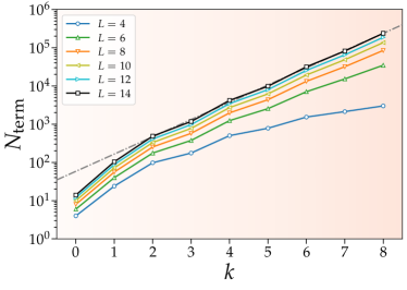
Figure 1: The number $N_{\rm term}$ of terms in the $\hat{O}_{k}$ operators as a function of $k$ for various system sizes $L$. The grey dash-dotted line indicates a line of $N_{\rm term}=10^{ak+b}$ with $a=0.4512$ and $b=1.7678$.

IV Numerical Results

IV.1 Physical quantities

Let us first summarize quantities calculated in our numerical simulations. Our primary concern is the time evolution of fidelities defined by

$$\begin{split}F_{tt}&=|\langle n(t)|\psi(t)\rangle|^{2},\\ F_{0t}&=|\langle n(0)|\psi(t)\rangle|^{2},\\ F_{Tt}&=|\langle n(T)|\psi(t)\rangle|^{2}.\\ \end{split}$$ (42)

Here $F_{tt}$ is the overlap between the instantaneous eigenstate $|n(t)\rangle$ of the UA model $\hat{H}(t)$, and the time-evolved state $|\psi(t)\rangle$ driven by either the UA or CD model. Accordingly, $F_{0t}$ ($F_{Tt}$) is the overlap between the instantaneous eigenstate of the initial (final) Hamiltonian and the time-evolved state. In this study, the initial state at $t=0$ is set to be the ground state of $\hat{H}(t=0)=\hat{H}_{\rm CD}^{(l)}(t=0)$, and thus $|\psi(t=0)\rangle=|n(t=0)\rangle$, which is nothing but the ground state of the noninteracting fermions. At the final time of the evolution, i.e., at $t=T$, the UA and CD models are again the same, $\hat{H}(t=T)=\hat{H}_{\rm CD}^{(l)}(t=T)$, and $|n(t=T)\rangle$ is the ground state of the Hubbard model $\hat{H}_{\rm HB}$. The fidelity $F_{tt}$ at $t=T$, denoted simply as $F_{TT}$, characterizes how faithfully we have prepared the ground state of the target Hubbard model.

In addition, we examine the time evolution of the lowest two eigenvalues, $E_{0}$ and $E_{1}$, of the UA and CD models with the associated spectrum gap $\Delta E=E_{1}-E_{0}$, the variational parameters $\{\alpha_{k}\}$, and the magnitudes of AGP terms, $\{M_{k}\}$, quantified by $M_{k}=\dot{\lambda}|\alpha_{k}|\cdot||\hat{O}_{2k-1}||_{\text{F}}$.

IV.2 System-size dependence at half filling

In accordance with the global U(1) symmetries for the charge and the spin sectors of the UA and CD models discussed in Sec. III.1, we compute the time evolution in each sector with the fixed numbers of up and down fermions, $N_{\uparrow}$ and $N_{\downarrow}$, respectively. Therefore, for even number $N_{f}$ of fermions, the sector with $N_{\uparrow}=N_{\downarrow}=N_{f}/2$, i.e., the total spin $S_{z}=0$, has the largest Hilbert space dimension $D=\binom{L}{N_{\uparrow}}\binom{L}{N_{\downarrow}}$. In this section, we focus on half filling, i.e., $N_{f}=L$, at which it is known that $S_{z}=0$ for the ground state of $\hat{H}(t=0)$ as well as $\hat{H}(t=T)$ for even $L$ under open-boundary conditions.

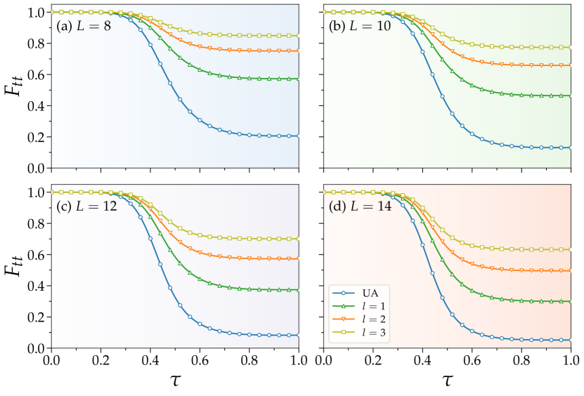
Figure 2: The time evolution of fidelity $F_{tt}$ for the UA model and the CD models with different driving orders $l=1,2,3$ on the 1D chains of (a) $L=8$, (b) $L=10$, (c) $L=12$ and (d) $L=14$ sites at half filling. The remaining parameters are $U=8$, $T=0.1$, $N_{T}=100$, $\Delta t=T/N_{T}=0.001$, and $N=10$. Here, time $t$ in the horizontal axis is scaled by the driving period $T$, i.e., $\tau=t/T$.

Figure 2 shows the time evolution of fidelity $F_{tt}$ with respect to the scaled time $\tau=t/T$ for the UA and CD ($l=1,2,3$) models with $U=8$ and different system sizes $L=8,10$, $12$, and $14$. Here, we choose the driving period $T=0.1$, $N_{T}=100$ with $\Delta t=T/N_{T}=0.001$, and the order of the Chebyshev polynomial expansion $N=10$. This set of parameters guarantees converged results [55]. It is clearly observed in Fig. 2 that, for each $L$, increasing $l$ remarkably improves the fidelity during the evolution. In the UA model, the final fidelities $F_{TT}$ at $t=T$ are 20.59%, 13.10%, 8.27%, and 5.19% for $L=8,10,12$, and $14$, respectively. These fidelities rapidly increase to 57.27%, 46.47%, 37.46%, and 30.04% when the first-order CD protocol is employed. The highest $F_{TT}$ achieved in the third-order CD protocol are 84.93%, 77.41%, 70.11%, and 63.20% for $L=8,10,12$, and $14$, respectively. Although we cannot continue to increase the order $l$ of the CD protocol any longer for these system sizes because of the computational cost, even better fidelity is expected for the higher-order CD protocol, as demonstrated in Fig. S3 for smaller systems sizes [55].

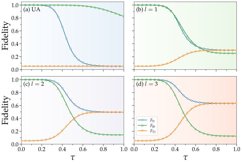
Figure 3: The time evolution of fidelities $F_{tt}$, $F_{0t}$, and $F_{Tt}$ for (a) the UA model and the CD models with (b) $l=1$, (c) $l=2$ and (d) $l=3$ on the 1D chain of $L=14$ sites at half filling. The remaining parameters are the same as in Fig. 2. Note that the results for $F_{tt}$ are exactly the same as those in Fig. 2(d).

Figure 3 shows the time evolution of the three different fidelities $F_{tt},F_{0t}$, and $F_{Tt}$ for the UA and CD ($l=1,2,3$) models on $L=14$ sites. In the UA case [Fig. 3(a)], $F_{0t}$ is very close to one for the first half of the driving period, i.e., $\tau<0.5$, and it remains to be a large value, as large as 82.27%, even at the end of driving period, i.e, $t=T$. On the other hand, $F_{Tt}$ is nearly constant throughout the whole driving period, i.e., $F_{Tt}\approx F_{TT}\,(=5.19$%) [see the orange line in Fig. 3(a)]. These results suggest that the time-evolved state $|\psi(t)\rangle$ for the UA model remains very close to the initial state $|n(0)\rangle$ until the end of the driving and, although $F_{tt}$ smoothly connects $F_{0t}$ at $t=0$ to $F_{Tt}$ at $t=T$, the time dependence of $F_{tt}$ arises essentially through the time dependence of $|n(t)\rangle$ itself, rather than $|\psi(t)\rangle$. Therefore, the UA model with the driving period $T=0.1$ is within an impulse regime where the driving period is too short for the system to response [61]. As shown in Figs. 3(b)-3(d), when the CD driving protocols are employed, the fidelity $F_{Tt}$ increases with time and reaches to significantly large values at the end of the driving period. Accordingly, the fidelity $F_{0t}$ dramatically decreases as the state $|\psi(t)\rangle$ evolves in time. The CD driving protocol by definition defies that the system is in an impulse regime, as demonstrated here for the cases with the driving period $T=0.1$. In fact, in the limit $l\to\infty$, the perfect final fidelity is anticipated, regardless of how short the driving period $T$ is (as a demonstration, see Fig. S4 in Ref. [55] for a smaller system with $L=6$).

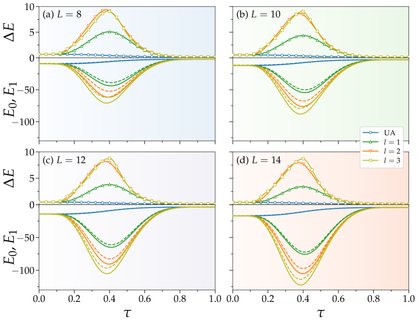
Figure 4: The time evolution of the lowest two eigenvalues $E_{0}$ and $E_{1}$, indicated by solid and dashed lines, respectively, in the lower panels and the corresponding spectrum gap $\Delta E$ in the upper panels for the UA and CD ($l=1,2,3$) models on the 1D chains of (a) $L=8$, (b) $L=10$, (c) $L=12$, and (d) $L=14$ sites at half filling. The remaining parameters are the same as in Fig. 2.

Figure 4 monitors the lowest two eigenvalues, $E_{0}$ and $E_{1}$, and the associated spectrum gap $\Delta E$ during the evolution for $L=8,10,12$, and $14$. In the UA model, the two eigenvalues monotonically increase with the evolution time, as shown by the solid and dashed blue lines in the lower panels of Figs. 4(a)-4(d), and the spectrum gap monotonically decreases, as shown in the upper panels. Hence, the maximal spectrum gap appears at the beginning of the evolution. In the CD models, the additional AGP terms first decrease the two eigenvalues to reach the minimal values and then retrieve the energies in the UA model at $t=T$, thus resulting in a valley shaped time-evolution of the spectrum. Importantly, the two eigenvalues decrease differently in slopes, i.e., the ground-state energy $E_{0}$ decreases steeper than the first-excited energy $E_{1}$, which yields an increase in the spectrum gap $\Delta E$. The gap maxima appear near the bottom of the spectrum valley. In the case of $L=14$, the maximal gap in the UA model is 0.4181, while it increases to 3.4122, 7.9891, and 8.7280 in the first-, second-, and third-order CD protocols, respectively. Nevertheless, we should note that in the case of $L=8$ shown in the upper panel of Fig. 4(a), the third-order CD protocol has the maximal spectrum gap $\Delta E=9.1050$ that is smaller than $\Delta E=9.3783$ of the second-order CD protocol, despite the fact that the better fidelity has been achieved for the third-order CD protocol throughout the evolution in Fig. 2(a).

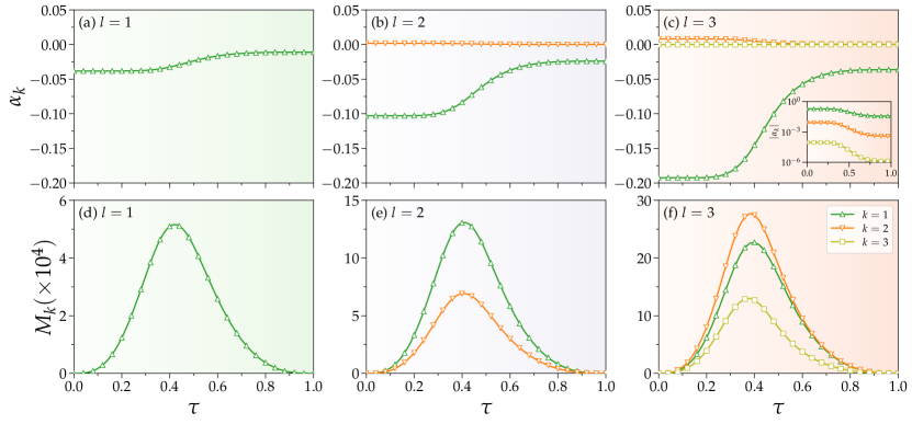
Figure 5: The time evolution of (a-c) the optimal variational parameters $\alpha_{k}$ and (d-f) the magnitudes $M_{k}$ of the corresponding AGP terms for the CD models with (a,d) $l=1$, (b,e) $l=2$, and (c,f) $l=3$. The results are obtained for $L=14$ at half filling. The remaining parameters are the same as in Fig. 2. The inset in (c) is a semi-logarithmic plot of $|\alpha_{k}|$, which demonstrates the exponential decrease of $|\alpha_{k}|$ in $k$.

Figure 5 shows the time evolution of the optimal variational parameters $\alpha_{k}$ and the magnitudes $M_{k}$ of the AGP terms for the CD ($l=1,2,3$) models on $L=14$ sites. First, we note that $\alpha_{1}$ is always negative for $l=1$, as $\alpha_{1}=-\Gamma_{1}/\Gamma_{2}<0$ [see Eq. (27)] is satisfied regardless of the Hamiltonian, and Fig. 5(a) indeed numerically confirms this behavior. Second, as discussed in Sec. II.4, we find that for a given order $l$ of the CD protocol, the absolute value $|\alpha_{k}|$ of the optimal variational parameter becomes exponentially smaller with increasing $k$ [see, e.g., the inset of Fig. 5(c)]. Third, likewise, we observe that $\Gamma_{k}$ increases exponentially in $k$. For example, as shown in Fig. 5(f), $M_{k}$ exhibits the maxima near $\tau=0.4$ for $l=3$, at which we find that $(|\alpha_{1}|,|\alpha_{2}|,|\alpha_{3}|)\sim(1\times 10^{-1},5\times 10^{-3},5\times 10^{-5})$ and $(\Gamma_{1},\Gamma_{3},\Gamma_{5})\sim(5\times 10^{9},7\times 10^{12},2\times 10^{16})$. As a result, the magnitudes $M_{k}$ for different $k$ values are in the same order, indicating that the higher-order terms in the approximated AGP also have significant contributions to the CD driving even though $|\alpha_{k}|$ is exponentially small for large $k$.

IV.3 Filling dependence

Figure 6 shows the time evolution of fidelity $F_{tt}$ for the UA and CD ($l=1,2,3$) models with $U=8$ on $L=14$ sites occupied by different numbers of fermions, $N_{f}=6,8,10$ and $12$, which correspond to the Hilbert-space dimensions $D=132496,1002001,4008004$, and $9018009$, respectively, assuming that $N_{\uparrow}=N_{\downarrow}$. Similarly to the cases at half filling, we find that the higher order $l$ of the CD model yields the better fidelity, which also demonstrates the universal usefulness of the CD protocol to the fermionic Hubbard model. In the UA model, we find that the final fidelity $F_{TT}$ decreases with increasing $N_{f}$ toward half filling. This is expected because the initial state $|\psi(0)\rangle=|n(0)\rangle$, which is the ground state of $\hat{H}_{J}$, better approximates the less-correlated target state. Remarkably, however, the improvement of the fidelity with increasing $l$ is most significant for $N_{f}=12$, despite the largest dimension of the Hilbert space. For example, while the final fidelities for $N_{f}=6$ are $51.39\%$, $63.59\%$, $73.32\%$, and $79.09\%$ for the UA model and the CD models with $l=1$, 2, and 3, respectively, those for $N_{f}=12$ are $17.37\%$, $59.85\%$, $77.03\%$, and $83.94\%$, respectively, indicating that the $N_{f}=12$ cases achieve even better final fidelities than the $N_{f}=6$ cases for $l=2$ and $3$. These results suggest that, while the fidelity improves systematically in the order $l$ of the CD model, irrespectively of $N_{f}$ or $D$, the effectiveness of the CD driving depends non-monotonically on $N_{f}$ and $D$.

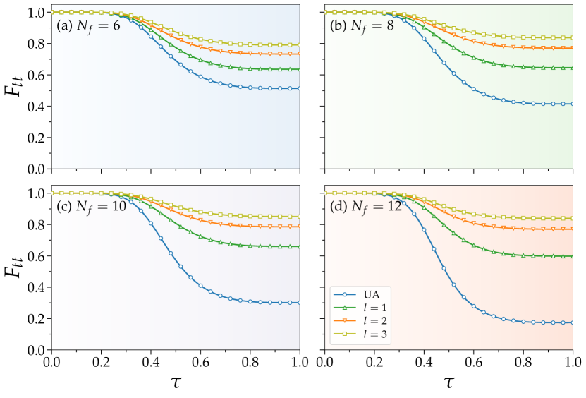
Figure 6: The time evolution of fidelity $F_{tt}$ for the UA model and the CD ($l=1,2,3$) models on the 1D chain of $L=14$ sites at different fermion fillings: (a) $N_{f}=6$, (b) $N_{f}=8$, (c) $N_{f}=10$, and (d) $N_{f}=12$. The results are obtained for the $S_{z}=0$ sector where the numbers of up and down fermions are equal, i.e., $N_{\uparrow}=N_{\downarrow}=N_{f}/2$. The remaining parameters are the same as in Fig. 2.

IV.4 $T$ and $U$ dependence

Figure 7 illustrates the final fidelity $F_{TT}$ as a function of the driving period $T$ for the UA and CD models with $U=8$ on $L=12$ sites at half filling. All the results indeed show a monotonic behavior where the smaller (larger) driving period $T$, i.e., faster (slower) driving, yields the worse (better) fidelity. Interestingly, we observe three distinct regimes: an adiabatic regime for $T\gtrsim T_{\text{adi}}\sim 10$, an impulse regime for $T\lesssim T_{\text{imp}}\sim 1.0$, and an intermediate regime for $T_{\text{imp}}\lesssim T\lesssim T_{\text{adi}}$  [61]. In the adiabatic regime, the time-evolved state accomplish almost perfect fidelity even for the UA model. It is well-known that the necessary condition for adiabaticity of quantum dynamics is given by

$$\sum_{m\,(\neq n)}\left|\frac{\langle m(t)|\partial_{t}n(t)\rangle}{\epsilon_{m}(t)-\epsilon_{n}(t)}\right|\ll 1$$ (43)

for $t\in[0,T]$, assuming that the initial state $|\psi(0)\rangle$ is in the $n$th instantaneous eigenstate $|n(0)\rangle$ of the initial Hamiltonian [62, 64, 63]. This implies that the characteristic time $T_{\text{adi}}$ in our setting is given by

$$T_{\rm adi}\approx\max_{\tau\in[0,1]}\left[\sum_{m\,(\neq n)}\left|\frac{\langle m(\tau)|\partial_{\tau}n(\tau)\rangle}{\epsilon_{m}(\tau)-\epsilon_{n}(\tau)}\right|\right]$$ (44)

with $n=0$, i.e., the instantaneous ground state of the Hamiltonian, and adiabaticity is fulfilled when $T\gtrsim T_{\text{adi}}$. Indeed, we find in Fig. 8 that $T_{\text{adi}}$ estimated from this criterion for the UA model is in good accordance with the crossover boundary between the intermediate and adiabatic regions shown in Fig. 7 (see Figs. S6 and S7 in Ref. [55] for the results with different values of $U$).

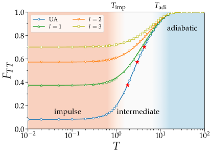
Figure 7: The final fidelity $F_{TT}$ as a function of the driving period $T$ for the UA and CD ($l=1,2,3$) models with $U=8$ on $L=12$ sites at half filling. For various $T$, the time step is fixed to be $\Delta t=0.001$. The three red stars on the curve for the UA model indicate the driving periods $T$ where the $F_{TT}$ values are equal to $F_{TT}$ at $T=0.1$ for the CD models with $l=1,2,$ and $3$. The three regimes, i.e., impulse, intermediate, and adiabatic regimes, distinguished by three different colors crossover between themselves around $T_{\text{imp}}$ and $T_{\text{adi}}$ indicated at the top of the figure.

On the other hand, in the impulse regime found in Fig. 7, the system is essentially frozen to stay in the initial state for the UA model [see Fig. 3(a)]. This is reasonable because in this region the driving is so fast that the system has little time to react. The characteristic time scale $T_{\text{imp}}$ below which the quantum state $|\psi(t)\rangle$ cannot follow the dynamics is determined approximately by the inverse of the spectrum gap $\Delta E$ ($=0.4822$ for $L=12$) at $t=0$, which is as large as $\sim 2.1$ for our case studied here (see Fig. S6 in Ref. [55] for the $U$ dependence). Moreover, it is highly intriguing to find that even in the fast driving regime $T\lesssim T_{\text{imp}}$, the higher order CD models can achieve better fidelity $F_{TT}$, suggesting that an extremely fast CD driving with $T\to 0^{+}$ is in principle possible without much deteriorating the fidelity, provided that the order $l$ of the CD models is large enough (see Fig. S4 in Ref. [55]). We also note that in the intermediate regime, the final fidelity $F_{TT}$ increases almost logarithmically with $T$ for the UA model as well as the CD models.

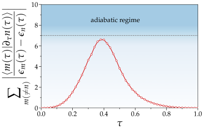
Figure 8: The time evolution of the quantity determining the adiabatic condition given in Eq. (44) for the UA model with $U=8$ on $L=12$ sites at half filling. This is evaluated by using the Lanczos-based method described in Ref. [55]. The dashed horizontal line is a guide for the eye.

To better understand how the CD protocol can speed up the driving process, we compare the fidelity $F_{TT}$ of the CD model with that of the UA model. Specifically, at $T=0.1$, the fidelity in the $l=1$ protocol is 37.46%. On the $F_{TT}-T$ curve for the UA model in Fig. 7, this fidelity can be reached for a much slower driving with $T=1.8$ (indicated by a red star in Fig. 7). In other words, the $l=1$ CD protocol realizes an 18 times speedup. Accordingly, the $l=2$ and $3$ CD protocols realize 30 and 43 times speedup, respectively, against the UA model to reach the corresponding fidelities $F_{TT}$ at $T=0.1$. Although the speedup depends on the driving period $T$, generally speaking, the CD protocol is more effective for the impulse regime where the UA model has a very low fidelity and the first oder CD driving already can significantly boost the fidelity. On the other hand, in the adiabatic regime, the fidelity $F_{TT}$ for the UA model is already close to unity, and hence the CD protocol is not necessary.

Figure 9 shows the final fidelity $F_{TT}$ as a function of the interaction strength $U$ for the UA and CD models on $L=12$ sites with the driving period $T=0.1$. At $U\ll 1$, where $\hat{H}_{U}$ can be considered as a perturbation to $\hat{H}_{J}$, the fidelity between the initial state $|\psi(0)\rangle=|n(0)\rangle$ and the target state $|n(T)\rangle$, i.e., the ground state of the Hubbard model $\hat{H}_{\rm HB}$, is already large, and hence the high fidelity can be achieved even for the UA model. On the other hand, as shown in Fig. 9, for $U\gg 1$, $F_{TT}$ dramatically decreases as expected. This implies that, in our setting of the UA and CD models in Eqs. (30) and (34), respectively, the ground state of the Hubbard model with large $U$ is much harder to prepare. For all the UA and CD protocols shown in Fig. 9, we also observe that there exist approximately two distinct regimes: a weak-correlation regime for $U\lesssim U_{c}\sim 7$ and a strong-correlation regime for $U\gtrsim U_{c}$. The CD protocol is more effective for the strong-correlation regime in the sense that it increases the final fidelity more significantly as compared with the UA protocol for the same $U$.

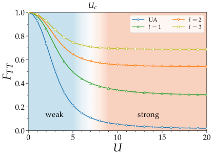
Figure 9: The final fidelity $F_{TT}$ as a function of the interaction strength $U$ for the UA and CD ($l=1,2,3$) models on $L=12$ sites at half filling. The remaining parameters are the same as in Fig. 2. Weak- and strong-correlation regimes crossover around $U_{c}$ indicated at the top of the figure.

V Conclusions

In summary, we have applied the variational CD driving protocol proposed in Ref. [40] to the 1D two-component fermionic Hubbard model. We have formalized the variational optimization procedure of the CD driving and shown that the optimal variational parameters are obtained deterministically by solving a set of linear equations whose coefficients are given by the squared Frobenius norms of the nested commutators $\hat{O}_{k}$. We have also devised an algorithm to construct analytical expressions of the nested commutators $\hat{O}_{k}$, which enables us to simulate systems up to $L=14$ sites with driving order $l\leqslant 3$. We have shown that the fidelity $F_{tt}$ dramatically increases with increasing $l$ throughout the evolution. Moreover, we have found that the CD driving protocol is more effective for the fast driving with the smaller driving period $T$ and the strong-correlation regime with the larger interaction strength $U$, where the increase of the final fidelity $F_{TT}$ is most significant when it is compared with the UA driving protocol.

Our results demonstrate the usefulness of the variational CD protocol for interacting fermions, and would be beneficial for further exploring fast ground-state preparation protocols for many-body fermionic systems, not only on classical computers but also on quantum devices in the foreseeable future. Indeed, establishing a variational-CD-inspired ansatz for the ground-state preparation of many-body systems on a quantum computer is an interesting issue to be addressed. A possible route for this is to combine the discretized quantum adiabatic process [65] with an efficient implementation of unitary operators generated by higher-order nested commutators [66].

Appendix A Proof of Eq. (24)

From Eq. (17), it is easy to verify

$$\text{Tr}\left(\hat{O}_{m}\hat{O}_{n}\right)=-\text{Tr}\left(\hat{O}_{m+1}\hat{O}_{n-1}\right).$$ (A.1)

This relation holds for $m\geq 0$ and $n\geq 1$, implying that $\text{Tr}\left(\hat{O}_{m}\hat{O}_{n}\right)=0$ when $n=m+1$. Then, using Eq. (18), one can readily show that

$$\left\langle\hat{O}_{2m},\hat{O}_{2k}\right\rangle_{\text{F}} =\text{Tr}\left(\hat{O}_{2m}^{\dagger}\hat{O}_{2k}\right)$$

$$=(-1)^{m+k}\text{Tr}\left(\hat{O}_{m+k}^{2}\right)$$

$$=\text{Tr}\left(\hat{O}_{m+k}^{\dagger}\hat{O}_{m+k}\right)$$

$$=\left|\left|\hat{O}_{m+k}\right|\right|_{\text{F}}^{2},$$ (A.2)

which thus proves Eq. (24).

Driving function

Figure S1 shows the driving function $\lambda(t)$ defined in Eq. (33) in the main text and its time derivative $\dot{\lambda}(t)$ in Eq. (35).

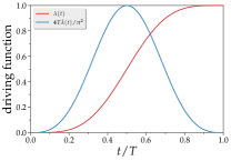
Figure S1: Driving function $\lambda(t)$ and its time derivative $\dot{\lambda}(t)$.

Direct approach

For small systems, we can take the direct approach, in which the $\hat{O}_{k}$ operators defined in Eq. (16) are treated by direct matrix-matrix multiplications recursively via Eq. (17). We use this approach as a benchmark to test the constructive approach described below.

Convergence and systematic error

Figure S2 compares the results of the fidelity for the UA model obtained by the full diagonalization method and the Chebyshev polynomial expansion method for small systems $L=6,7$, and $8$. Due to the small time interval $\Delta t=T/N_{T}=0.001$, a small Chebyshev expansion order $N=10$ is enough to obtain the converged results to the exact values. Note also that the systematic error due to the discretization of the time in the time-evolution operator [see Eq. (36) in the main text] is also negligible when $\Delta t$ is as small as 0.001, as shown in the left panels of Fig. S2.

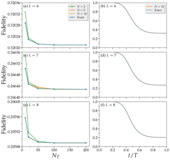
Figure S2: Comparison of the results obtained by the full diagonalization method and the Chebyshev polynomial expansion method for the UA model with $U=8$ on different system sizes $L=6,7$, and $8$ at half filling. Here the evolution period is set to be $T=0.1$. Left panels (a, c, e) show the final fidelity $F_{TT}$ as a function of the number $N_{T}$ of time steps. In the Chebyshev polynomial expansion method, three different expansion orders ($N=2,5$, and $10$) are used. Note that since the evolution period $T$ is fixed, the time interval $\Delta t=T/N_{T}$ becomes smaller with increasing $N_{T}$. Right panels (b, d, f) show the time evolution of fidelity $F_{tt}$. We set $N=10$ in the Chebyshev polynomial expansion method and $\Delta t=0.001$.

Numerical results for small systems

Figure S3 shows the time evolution of fidelity $F_{tt}$ for the UA and CD models with $U=8$ on small sites ($L=4,5,6$, and $7$) at half filling, i.e., $N_{f}=L$, with $N_{\uparrow}=N_{\downarrow}$ for even $N_{f}$ and $N_{\uparrow}=N_{\downarrow}+1$ for odd $N_{f}$. Here, we use the direct approach and set the driving period $T=0.1$. The higher-order CD protocols can be applied for these small systems, where the final fidelity $F_{TT}$ as well as $F_{tt}$ during the whole driving period approaches almost one, implying that essentially the perfect CD evolution is achieved.

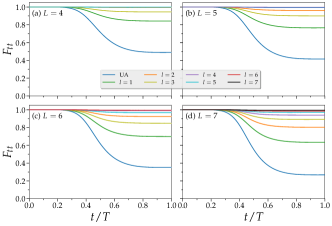
Figure S3: The time evolution of fidelity $F_{tt}$ for the UA model and the CD models with different orders $l$ on the 1D chains of (a) $L=4$, (b) $L=5$, (c) $L=6$, and (d) $L=7$ sites at half filling. In (b) and (d), $N_{\uparrow}=N_{\downarrow}+1$ and thus the total $S_{z}=1/2$. The remaining parameters are the same as in Fig. 2 in the main text. The largest final fidelities $F_{TT}$ are $99.80\%$, $99.73\%$, $99.49\%$, and $99.39\%$ for $L=4,5,6$, and $7$ with $l=4,5,6$, and $7$, respectively.

Figure S4 shows the final fidelity $F_{TT}$ as a function of the driving period $T$ for the UA and CD ($l=1,2,\cdots,6$) models with $U=8$ on $L=6$ sites at half filling calculated using the direct approach. Although the system size used here is smaller, we find that the crossover boundaries among the impulse, intermediate, and adiabatic regions are similar to those indicated in Fig. 7, for which the system size $L=12$ is considered. The spectrum gap $\Delta E$ for the UA model at $t=0$, which is the largest during the time evolution, is $0.8901$ for $L=6$. The characteristic time $T_{\rm adi}$ defined in Eq. (44) is $\sim 9$ for the UA model with $U=8$ on $L=6$ sites. We should also emphasize in Fig. S4 that the final fidelity $F_{TT}$ approaches to one with increasing the order $l$ for the CD model even when $T\to 0^{+}$.

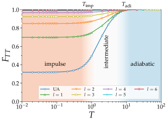
Figure S4: The final fidelity $F_{TT}$ as a function of the driving period $T$ for the UA and CD ($l=1,2,\cdots,6$) models with $U=8$ on $L=6$ sites at half filling. For various $T$, the time step is fixed to be $\Delta t=0.001$.

Constructive approach

As discussed in Sec. III.2.2, the UA and CD models are composed of the summation of multi-fermion-operator products of the form

$$\hat{h}_{m,x}=\lambda(t)^{m}\beta_{x}\hat{c}^{\dagger}_{i}\hat{c}^{\dagger}_{j}\cdots\hat{c}_{p}\hat{c}_{q}\cdots.$$ (S1)

We refer to each of these products as a Hamiltonian term. The total number $N_{\text{term}}$ of terms in the UA model $\hat{H}(t)$ scales linearly in the system size $L$. For instance, under open-boundary conditions, an $L$-site chain has $2(L-1)$ hopping terms for each spin and $L$ onsite interacting terms (assuming nonzero $J$ and $U$). Thus, $N_{\text{term}}=5L-4\sim\mathcal{O}(L)$.

There are three different conventions for the order of fermion operators in Hamiltonian terms: (1) general, (2) normal-ordered (NO), and (3) special normal-ordered (SNO) forms. In the general form, the creation and annihilation operators have no particular order. In the NO form, all creation operators are on the left of annihilation operators. In the SNO form, the creation and annihilation operators in a NO term are both ordered according to the indexes, e.g., $i<j<\cdots$ and $p<q<\cdots$.

A NO term can be transformed into a SNO term by simple permutations. Except for a possible minus sign due to the anticommutative relation (i.e., $\hat{c}^{\dagger}_{j}\hat{c}^{\dagger}_{i}=-\hat{c}^{\dagger}_{i}\hat{c}^{\dagger}_{j}$, $\hat{c}_{q}\hat{c}_{p}=-\hat{c}_{p}\hat{c}_{q}$ ), no additional term arises. However, when one transforms a general term into the NO form, many additional terms emerge in general because $\hat{c}_{i}\hat{c}^{\dagger}_{j}=\delta_{ij}-\hat{c}^{\dagger}_{j}\hat{c}_{i}$. Here we devise an algorithm to implement the transformation among these three different forms of Hamiltonian terms, and thus we are able to compute the commutator $\hat{O}_{k}=[\hat{H},\hat{O}_{k-1}]$ in an analytic representation.

We now describe the constructive approach, which has been implemented in our code available at [1]. Before the time-evolution calculation,

1. We build the analytical representation of the UA model $\hat{H}(t)$. The hopping part $\hat{H}_{J}$ has $m=0$ and the interacting part $\lambda(t)\hat{H}_{U}$ has $m=1$.

2. The $\hat{O}_{k}$ operators for $k=1,2,\cdots,2l$ are constructed recursively starting with $\hat{O}_{0}=\hat{H}_{U}$.

3. All the diagonal terms in $\hat{O}_{k}^{\dagger}\hat{O}_{k}$ are constructed.

4. The $S^{k,m}$ are calculated for $1\leqslant k\leqslant 2l$ and $0\leqslant m\leqslant 2l-1$ by tracing the diagonal terms in $\hat{O}_{k}^{\dagger}\hat{O}_{k}$ over the many-body bases.

5. The initial model $\hat{H}(t=0)=\hat{H}_{\text{CD}}^{(l)}(t=0)$ is constructed and the initial state $|\psi(t=0)\rangle=|n(t=0)\rangle$, i.e., the ground state of $\hat{H}(t=0)$, is calculated.

6. The ground state $|n(t=T)\rangle$ of $\hat{H}(t=T)=\hat{H}_{\text{CD}}^{(l)}(t=T)$ at the final time $T$ is also calculated by using the Lanczos algorithm [2] for the evaluation of $F_{Tt}$.

The detailed procedure at each time step $t_{i}$ is as follows. Staring with $i=1$ and setting $t_{i=0}=0$ and $t_{i=1}=\Delta t$,

1. The time-evolved state $|\psi(t_{i})\rangle$ is calculated through $|\psi(t_{i})\rangle=e^{-i\Delta t\hat{H}[\lambda(t_{i-1})]}|\psi(t_{i-1})\rangle$ by using the Chebyshev polynomial expansion method. The lowest two eigenvalues of $\hat{H}(t_{i})$ are calculated by using the block-Lanczos algorithm [3], if necessary. The same procedure is applied for the CD model $\hat{H}_{\rm CD}^{(l)}$ by replacing $\hat{H}$ with $\hat{H}_{\rm CD}^{(l)}$.

2. The UA model $\hat{H}(t_{i})$ is constructed.

3. The ground state $|n(t_{i})\rangle$ of $\hat{H}(t_{i})$ is calculated by using the Lanczos algorithm.

4. Fidelities $F_{tt}$, $F_{0t}$ and $F_{Tt}$ are calculated. If $t_{i}=T$, exit.

5. $\Gamma_{k}$ in Eq. (41) are calculated for $1\leqslant k\leqslant 2l$ by using $S^{k,m}$ already evaluated in step 4.

6. The optimal parameters $\alpha_{k}$ ($k=1,2,\ldots,l$) are obtained by solving the set of the linear equations in Eq. (27).

7. An analytical form of $\hat{H}_{\text{CD}}^{(l)}(t_{i})$ is constructed by adding the AGP terms $i\dot{\lambda}\alpha_{k}\hat{O}_{2k-1}$ with $k=1,2,\ldots,l$ to $\hat{H}(t_{i})$.

8. Go back to Step 7 with the next time step $t_{i}\rightarrow t_{i+1}=t_{i}+\Delta t$.

As an example, we show the analytical forms of $\hat{H}[\lambda(T)=1]=\hat{H}_{\text{HB}}$ and $\hat{O}_{k}[\lambda(T)=1]$ operators for $L=2$ and $l=1$ generated by our code available at [1]. The Hubbard model $\hat{H}_{\text{HB}}$ with $U=8$ is given by

6
c+ 1  c 2          0    -0.100000E+01   0.000000E+00
c+ 2  c 1          0    -0.100000E+01   0.000000E+00
c+ 3  c 4          0    -0.100000E+01   0.000000E+00
c+ 4  c 3          0    -0.100000E+01   0.000000E+00
c+ 1 c+ 3  c 1  c 3          1    -0.800000E+01  -0.000000E+00
c+ 2 c+ 4  c 2  c 4          1    -0.800000E+01  -0.000000E+00

The $\hat{O}_{k}$ operators are given by

$\hat{O}_{0}=\hat{H}_{U}$:

2
c+ 1 c+ 3  c 1  c 3          0    -0.800000E+01  -0.000000E+00
c+ 2 c+ 4  c 2  c 4          0    -0.800000E+01  -0.000000E+00

$\hat{O}_{1}=[\hat{H},\hat{O}_{0}]$:

8
c+ 1 c+ 3  c 1  c 4          0    -0.800000E+01  -0.000000E+00
c+ 1 c+ 3  c 2  c 3          0    -0.800000E+01  -0.000000E+00
c+ 1 c+ 4  c 1  c 3          0     0.800000E+01   0.000000E+00
c+ 1 c+ 4  c 2  c 4          0     0.800000E+01   0.000000E+00
c+ 2 c+ 3  c 1  c 3          0     0.800000E+01   0.000000E+00
c+ 2 c+ 3  c 2  c 4          0     0.800000E+01   0.000000E+00
c+ 2 c+ 4  c 1  c 4          0    -0.800000E+01  -0.000000E+00
c+ 2 c+ 4  c 2  c 3          0    -0.800000E+01  -0.000000E+00

$\hat{O}_{2}=[\hat{H},\hat{O}_{1}]$:

20
c+ 1 c+ 3  c 1  c 3          0    -0.320000E+02   0.000000E+00
c+ 1 c+ 3  c 2  c 4          0    -0.320000E+02   0.000000E+00
c+ 1 c+ 4  c 1  c 4          0     0.320000E+02   0.000000E+00
c+ 1 c+ 4  c 2  c 3          0     0.320000E+02   0.000000E+00
c+ 2 c+ 3  c 1  c 4          0     0.320000E+02   0.000000E+00
c+ 2 c+ 3  c 2  c 3          0     0.320000E+02   0.000000E+00
c+ 2 c+ 4  c 1  c 3          0    -0.320000E+02   0.000000E+00
c+ 2 c+ 4  c 2  c 4          0    -0.320000E+02   0.000000E+00
c+ 1 c+ 3  c 1  c 4          1    -0.640000E+02  -0.000000E+00
c+ 1 c+ 3  c 2  c 3          1    -0.640000E+02  -0.000000E+00
c+ 1 c+ 4  c 1  c 3          1    -0.640000E+02  -0.000000E+00
c+ 1 c+ 4  c 2  c 4          1    -0.640000E+02  -0.000000E+00
c+ 2 c+ 3  c 1  c 3          1    -0.640000E+02  -0.000000E+00
c+ 2 c+ 3  c 2  c 4          1    -0.640000E+02  -0.000000E+00
c+ 2 c+ 4  c 1  c 4          1    -0.640000E+02  -0.000000E+00
c+ 2 c+ 4  c 2  c 3          1    -0.640000E+02  -0.000000E+00
c+ 1 c+ 2 c+ 3  c 1  c 2  c 4          1     0.128000E+03   0.000000E+00
c+ 1 c+ 2 c+ 4  c 1  c 2  c 3          1     0.128000E+03   0.000000E+00
c+ 1 c+ 3 c+ 4  c 2  c 3  c 4          1     0.128000E+03   0.000000E+00
c+ 2 c+ 3 c+ 4  c 1  c 3  c 4          1     0.128000E+03   0.000000E+00

The integer in the front line counts the number of terms $N_{\text{term}}$. c+ and c denote creation and annihilation operators, respectively. The integers following c+ and c are collective indexes of sites and spins. In this example, 1 (3) labels the spin up (down) on the first site and 2 (4) labels the spin up (down) on the second site. The last two real numbers are the real and imaginary parts of the coefficient $\beta_{x}$. The integer before $\beta_{x}$ is $m$.

We also provide an example for $S^{k,m}$ generated by our code available at [1]. The $S^{k,m}$ for $L=14$, $N_{f}=14$, $N_{\uparrow}=7$, and $l=3$ with $U=8$ are given by

1.000000    8.000000  # J, U
14   14    7    7     # L, Nf, Nup, Ndn
3                     # driving order l

Gamma1
S(1,0) =    0.568273305600000E+10

Gamma2
S(2,0) =    0.148625326080000E+12
S(2,1) =    0.363694915584000E+12

Gamma3
S(3,0) =    0.533652347289600E+13
S(3,1) =    0.230526623416320E+14
S(3,2) =    0.232764745973760E+14

Gamma4
S(4,0) =    0.222388949680128E+15
S(4,1) =    0.137124173787955E+16
S(4,2) =    0.259980316272230E+16
S(4,3) =    0.148969437423206E+16

Gamma5
S(5,0) =    0.101046765965967E+17
S(5,1) =    0.816746874273792E+17
S(5,2) =    0.227024409238438E+18
S(5,3) =    0.254852329868624E+18
S(5,4) =    0.953404399508521E+17

Gamma6
S(6,0) =    0.485832012237767E+18
S(6,1) =    0.491237560046164E+19
S(6,2) =    0.182253012110310E+20
S(6,3) =    0.304507281118027E+20
S(6,4) =    0.230283831881289E+20
S(6,5) =    0.610178815685453E+19

Here, Gamma1, Gamma2, etc. denote $\Gamma_{1}$, $\Gamma_{2}$, etc., respectively, and only nonzero $S^{k,m}$ are shown.

Benchmark tests

Figure S5 compares the results for the time evolution of the fidelity $F_{tt}$ obtained by the direct and constructive approaches for the UA and CD ($l=1,2$) models with $U=8$ on $L=7$ and $8$ sites at half filling. As is expected, these two results are exactly the same within the numerical precision.

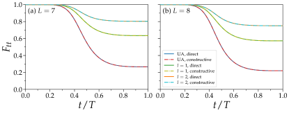
Figure S5: Comparison of the results for the time evolution of the fidelity $F_{tt}$ obtained by the direct and constructive approaches for the UA and CD ($l=1,2$) models with $U=8$ on (a) $L=7$ and (b) $L=8$ sites at half filling. In (a), we set $N_{\uparrow}=N_{\downarrow}+1$. The remaining parameters are the same as in Fig. 2 in the main text.

$U$ dependence of $T_{\rm adi}$

Figure S6 shows the $U$ dependence of the final fidelity $F_{TT}$ as a function of the driving period $T$ for the UA model on $L=12$ sites at half filling. Although the crossover boundary between the impulse and intermediate regions is insensitive to the value of the interaction strength $U$, the crossover boundary between the intermediate and adiabatic regions depend slightly on $U$. The latter is in accordance with the $U$ dependence of the characteristic time $T_{\rm adi}$ defined in Eq. (44), i.e., $T_{\rm adi}\sim 2,4,7$, and $10$ for $U=2,4,8$, and $16$, respectively (see Fig. S7). Indeed, the quantity in the right hand side of Eq. (44) can also be written as

$$\left|\frac{\langle m(\tau)|\partial_{\tau}n(\tau)\rangle}{\epsilon_{m}(\tau)-\epsilon_{n}(\tau)}\right|=\frac{\left|\langle m(\tau)|\partial_{\tau}\hat{H}(\tau)|n(\tau)\rangle\right|}{[\epsilon_{m}(\tau)-\epsilon_{n}(\tau)]^{2}}=\partial_{\tau}\lambda(\tau)\frac{\left|\langle m(\tau)|\hat{H}_{U}|n(\tau)\rangle\right|}{[\epsilon_{m}(\tau)-\epsilon_{n}(\tau)]^{2}}=U\partial_{\tau}\lambda(\tau)\frac{\left|\langle m(\tau)|\hat{D}|n(\tau)\rangle\right|}{[\epsilon_{m}(\tau)-\epsilon_{n}(\tau)]^{2}},$$ (S2)

where $\partial_{\tau}\lambda(\tau)=T\dot{\lambda}(t)$ and $\hat{D}=\sum_{i}\hat{n}_{i\uparrow}\hat{n}_{i\downarrow}$, and therefore Eq. (44) is now

$$T_{\rm adi}\approx\max_{\tau\in[0,1]}\left[U\partial_{\tau}\lambda(\tau)\sum_{m\,(\neq n)}\frac{\left|\langle m(\tau)|\hat{D}|n(\tau)\rangle\right|}{[\epsilon_{m}(\tau)-\epsilon_{n}(\tau)]^{2}}\right].$$ (S3)

This implies that the characteristic time $T_{\rm adi}$ separating the intermediate and adiabatic regions is approximately proportional to $U$, assuming that other quantities in Eq. (S3) do not depend strongly on $U$, which is however not the case when $U$ is very large.

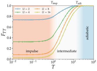
Figure S6: The final fidelity $F_{TT}$ as a function of the driving period $T$ for the UA model with $U=2,4,8$, and $16$ on $L=12$ sites at half filling. For various $T$, the time step is fixed to be $\Delta t=0.001$. Notice that the results for $U=8$ are the same as those shown in Fig. 7.

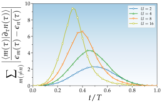
Figure S7: The time evolution of the quantity determining the adiabatic condition given in Eq. (44) for the UA model with $U=2,4,8$, and $16$ on $L=12$ sites at half filling.

Lanczos-based method for the evaluation of Eq. (44)

Here, we describe a Lanczos-based method to evaluate the quantity $\sum_{m\,(\neq n)}\left|\frac{\langle m(\tau)|\partial_{\tau}n(\tau)\rangle}{\epsilon_{m}(\tau)-\epsilon_{n}(\tau)}\right|$ in the right hand side of Eq. (44) through the relation in Eq. (S2). At each time step $t_{i}$, the quantity $\sum_{m\,(\neq n)}\frac{|\langle m(t_{i})|\hat{D}|n(t_{i})\rangle|}{[\epsilon_{m}(t_{i})-\epsilon_{n}(t_{i})]^{2}}$ with $n=0$, i.e., the instantaneous ground state of the UA model, can be evaluated as following (the time $t_{i}$ dependence is abbreviated for simplicity):

1. First calculate the ground state $|0\rangle$ and its associated energy $\epsilon_{0}$ of the UA model $\hat{H}(t_{i})$.

2. Prepare the state $|\phi_{0}\rangle=\hat{D}|0\rangle$.

3. Compute the normlization constant $N_{0}=\sqrt{\langle\phi_{0}|\phi_{0}\rangle}$.

4. Run an $M$-step Lanczos iteration for the UA model $\hat{H}(t_{i})$, starting with the normalized vector

   $$|\tilde{\phi}_{0}\rangle=|\phi_{0}\rangle/N_{0},$$ (S4)

   and obtain the resultant $M\times M$ tridiagonal matrix ${\bf T}$, which is an approximate matrix representation of the UA model $\hat{H}(t_{i})$ in the $M$-dimensional Krylov subspace.

5. Diagonalize the tridiagonal matrix ${\bf T}$ to obtain the eigenvalues $\{{\tilde{\epsilon}_{l}\}_{l=0}^{M-1}}$ and the associated eigenvectors $\{{\bf v}_{l}\}_{l=0}^{M-1}$.

6. The desired quantity can be evaluated approximately as

   $$\sum_{m\,(\neq 0)}\frac{\left|\langle m|\hat{D}|0\rangle\right|}{(\epsilon_{m}-\epsilon_{0})^{2}}\approx N_{0}\sum_{l=1}^{M-1}\frac{\left|[{\bf v}_{l}]_{0}\right|}{(\tilde{\epsilon}_{l}-\epsilon_{0})^{2}}.$$ (S5)

   Here $[{\bf v}_{l}]_{0}$ is the first entry of the $l$th eigenvector and it represents the overlap between the $l$th eigenvector ${\bf v}_{l}$ and the normalized initial vector $|\tilde{\phi}_{0}\rangle$ [see, for example, Eq. (81) in Ref. [4]].

We demonstrate this method for a small system with $L=6$ sites and compare the results with those obtained by the numerically exact full diagonalization method in Fig. S8.

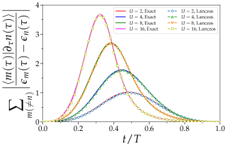
Figure S8: Comparison of the results for the time evolution of the quantity determining the adiabatic condition given in Eq. (44) calculated by the Lanczos method and the numerically exact full diagonalization method for the UA model with $U=2,4,8$, and $16$ on $L=6$ sites at half filling.

Fidelity of the CD model

It is also interesting to examine the time evolution of the fidelity $F^{\text{CD}}_{tt}$ for the CD model $\hat{H}_{\rm CD}^{(l)}$ defined by $F^{\text{CD}}_{tt}=|\langle n^{\text{CD}}(t)|\psi(t)\rangle|^{2}$, where $|n^{\text{CD}}(t)\rangle$ and $|\psi(t)\rangle$ are the instantaneous eigenstate and the time-evolved state of the CD model, respectively. Figure S9 shows the results for the CD model with $l=3$ on the 1D chain of $L=12$ sites at half filling.

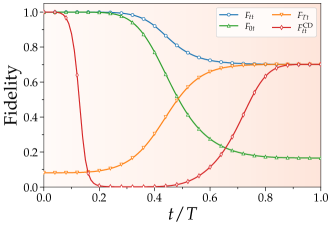
Figure S9: The time evolution of fidelity $F^{\text{CD}}_{tt}$ for the CD model with $l=3$ on the 1D chain of $L=12$ sites at half filling. The remaining parameters are the same as in Fig. 2. For comparison, the results for other fidelities $F_{tt}$, $F_{0t}$, and $F_{Tt}$ are also shown.

References

- [1] M. A. Nielsen and I. L. Chuang, Quantum Computation and Quantum Information: 10th Anniversary Edition, (2010).
- [2] T. Albash and D. A. Lidar, Adiabatic Quantum Computation, Rev. Mod. Phys. 90, 015002 (2018).
- [3] C. E. Wieman, D. E. Pritchard, and D. J. Wineland, Atom Cooling, Trapping, and Quantum Manipulation, Rev. Mod. Phys. 71, S253 (1999).
- [4] T. Kato, On the Adiabatic Theorem of Quantum Mechanics, J. Phys. Soc. Jpn. 5, 435 (1950).
- [5] E. A. Coello Pérez, J. Bonitati, D. Lee, S. Quaglioni, and K. A. Wendt, Quantum State Preparation by Adiabatic Evolution with Custom Gates, Phys. Rev. A 105, 032403 (2022).
- [6] M. Khazali and K. Mølmer, Fast Multiqubit Gates by Adiabatic Evolution in Interacting Excited-State Manifolds of Rydberg Atoms and Superconducting Circuits, Phys. Rev. X 10, 021054 (2020).
- [7] X. Chen, A. Ruschhaupt, S. Schmidt, A. del Campo, D. Guéry-Odelin, and J. G. Muga, Fast Optimal Frictionless Atom Cooling in Harmonic Traps: Shortcut to Adiabaticity, Phys. Rev. Lett. 104, 063002 (2010).
- [8] D. Guéry-Odelin, A. Ruschhaupt, A. Kiely, E. Torrontegui, S. Martínez-Garaot, and J. G. Muga, Shortcuts to Adiabaticity: Concepts, Methods, and Applications, Rev. Mod. Phys. 91, 045001 (2019).
- [9] S. Masuda and K. Nakamura, Fast-Forward Problem in Quantum Mechanics, Phys. Rev. A 78, 062108 (2008).
- [10] S. Masuda and K. Nakamura, Fast-Forward of Adiabatic Dynamics in Quantum Mechanics, Proc. R. Soc. A 466, 1135 (2010).
- [11] N. V. Vitanov, T. Halfmann, B. W. Shore, and K. Bergmann, LASER-INDUCED POPULATION TRANSFER BY ADIABATIC PASSAGE TECHNIQUES, Annu. Rev. Phys. Chem. 52, 763 (2001).
- [12] F. Vewinger, J. Appel, E. Figueroa, and A. I. Lvovsky, Adiabatic Frequency Conversion of Optical Information in Atomic Vapor, Opt. Lett. 32, 2771 (2007).
- [13] Y. P. Kandel, H. Qiao, S. Fallahi, G. C. Gardner, M. J. Manfra, and J. M. Nichol, Adiabatic Quantum State Transfer in a Semiconductor Quantum-Dot Spin Chain, Nat. Commun. 12, 2156 (2021).
- [14] B. B. Zhou, A. Baksic, H. Ribeiro, C. G. Yale, F. J. Heremans, P. C. Jerger, A. Auer, G. Burkard, A. A. Clerk, and D. D. Awschalom, Accelerated Quantum Control Using Superadiabatic Dynamics in a Solid-State Lambda System, Nat. Phys. 13, 330 (2017).
- [15] R. R. Agundez, C. D. Hill, L. C. L. Hollenberg, S. Rogge, and M. Blaauboer, Superadiabatic Quantum State Transfer in Spin Chains, Phys. Rev. A 95, 012317 (2017).
- [16] A. Vepsäläinen, S. Danilin, and G. S. Paraoanu, Superadiabatic Population Transfer in a Three-Level Superconducting Circuit, Sci. Adv. 5, eaau5999 (2019).
- [17] U. Gaubatz, P. Rudecki, S. Schiemann, and K. Bergmann, Population Transfer Between Molecular Vibrational Levels by Stimulated Raman Scattering with Partially Overlapping Laser Fields. A New Concept and Experimental Results, J. Chem. Phys. 92, 5363 (1990).
- [18] K. Bergmann, H. Theuer, and B. W. Shore, Coherent Population Transfer Among Quantum States of Atoms and Molecules, Rev. Mod. Phys. 70, 1003 (1998).
- [19] A. D. Greentree, J. H. Cole, A. R. Hamilton, and L. C. L. Hollenberg, Coherent Electronic Transfer in Quantum Dot Systems Using Adiabatic Passage, Phys. Rev. B 70, 235317 (2004).
- [20] N. V. Vitanov, A. A. Rangelov, B. W. Shore, and K. Bergmann, Stimulated Raman Adiabatic Passage in Physics, Chemistry, and Beyond, Rev. Mod. Phys. 89, 015006 (2017).
- [21] J. Preskill, Quantum Computing in the NISQ Era and Beyond, Quantum 2, 79 (2018).
- [22] F. Arute, K. Arya, R. Babbush, D. Bacon, J. C. Bardin, R. Barends, R. Biswas, S. Boixo, F. G. S. L. Brandao, D. A. Buell, B. Burkett, Y. Chen, Z. Chen, B. Chiaro, R. Collins, W. Courtney, A. Dunsworth, E. Farhi, B. Foxen, A. Fowler, C. Gidney, M. Giustina, R. Graff, K. Guerin, S. Habegger, M. P. Harrigan, M. J. Hartmann, A. Ho, M. Hoffmann, T. Huang, T. S. Humble, S. V. Isakov, E. Jeffrey, Z. Jiang, D. Kafri, K. Kechedzhi, J. Kelly, P. V. Klimov, S. Knysh, A. Korotkov, F. Kostritsa, D. Landhuis, M. Lindmark, E. Lucero, D. Lyakh, S. Mandrà, J. R. McClean, M. McEwen, A. Megrant, X. Mi, K. Michielsen, M. Mohseni, J. Mutus, O. Naaman, M. Neeley, C. Neill, M. Y. Niu, E. Ostby, A. Petukhov, J. C. Platt, C. Quintana, E. G. Rieffel, P. Roushan, N. C. Rubin, D. Sank, K. J. Satzinger, V. Smelyanskiy, K. J. Sung, M. D. Trevithick, A. Vainsencher, B. Villalonga, T. White, Z. J. Yao, P. Yeh, A. Zalcman, H. Neven, and J. M. Martinis, Quantum Supremacy Using a Programmable Superconducting Processor, Nature 574, 505 (2019).
- [23] K. Bharti, A. Cervera-Lierta, T. H. Kyaw, T. Haug, S. Alperin-Lea, A. Anand, M. Degroote, H. Heimonen, J. S. Kottmann, T. Menke, W.-K. Mok, S. Sim, L.-C. Kwek, and A. Aspuru-Guzik, Noisy Intermediate-Scale Quantum Algorithms, Rev. Mod. Phys. 94, 015004 (2022).
- [24] P. Ball, First Quantum Computer to Pack 100 Qubits Enters Crowded Race, Nature 599, 542 (2021).
- [25] A. C. Santos, R. D. Silva, and M. S. Sarandy, Shortcut to Adiabatic Gate Teleportation, Phys. Rev. A 93, 012311 (2016).
- [26] E. Boyers, M. Pandey, D. K. Campbell, A. Polkovnikov, D. Sels, and A. O. Sushkov, Floquet-Engineered Quantum State Manipulation in a Noisy Qubit, Phys. Rev. A 100, 012341 (2019).
- [27] J. Yao, L. Lin, and M. Bukov, Reinforcement Learning for Many-Body Ground-State Preparation Inspired by Counterdiabatic Driving, Phys. Rev. X 11, 031070 (2021).
- [28] A. Hartmann and W. Lechner, Rapid Counter-Diabatic Sweeps in Lattice Gauge Adiabatic Quantum Computing, New J. Phys. 21, 043025 (2019).
- [29] N. N. Hegade, K. Paul, Y. Ding, M. Sanz, F. Albarrán-Arriagada, E. Solano, and X. Chen, Shortcuts to Adiabaticity in Digitized Adiabatic Quantum Computing, Phys. Rev. Applied 15, 024038 (2021).
- [30] N. N. Hegade, P. Chandarana, K. Paul, X. Chen, F. Albarrán-Arriagada, and E. Solano, Portfolio Optimization with Digitized-Counterdiabatic Quantum Algorithms, arXiv:2112.08347.
- [31] J. Wurtz and P. J. Love, Counterdiabaticity and the Quantum Approximate Optimization Algorithm, Quantum 6, 635 (2022).
- [32] P. Chandarana, N. N. Hegade, K. Paul, F. Albarrán-Arriagada, E. Solano, A. del Campo, and X. Chen, Digitized-Counterdiabatic Quantum Approximate Optimization Algorithm, Phys. Rev. Research 4, 013141 (2022).
- [33] S. H. Sack and M. Serbyn, Quantum Annealing Initialization of the Quantum Approximate Optimization Algorithm, Quantum 5, 491 (2021).
- [34] N. N. Hegade, X. Chen, and E. Solano, Digitized-Counterdiabatic Quantum Optimization, arXiv:2201.00790.
- [35] M. Demirplak and S. A. Rice, Adiabatic Population Transfer with Control Fields, J. Phys. Chem. A 107, 9937 (2003).
- [36] M. Demirplak and S. A. Rice, Assisted Adiabatic Passage Revisited, J. Phys. Chem. B 109, 6838 (2005).
- [37] M. Demirplak and S. A. Rice, On the Consistency, Extremal, and Global Properties of Counterdiabatic Fields, J. Chem. Phys. 129, 154111 (2008).
- [38] A. del Campo, Shortcuts to Adiabaticity by Counterdiabatic Driving, Phys. Rev. Lett. 111, 100502 (2013).
- [39] M. V. Berry, Transitionless Quantum Driving, J. Phys. A: Math. Theor. 42, 365303 (2009).
- [40] P. W. Claeys, M. Pandey, D. Sels, and A. Polkovnikov, Floquet-Engineering Counterdiabatic Protocols in Quantum Many-Body Systems, Phys. Rev. Lett. 123, 090602 (2019).
- [41] G. Passarelli, V. Cataudella, R. Fazio, and P. Lucignano, Counterdiabatic Driving in the Quantum Annealing of the -Spin Model: A Variational Approach, Phys. Rev. Research 2, 013283 (2020).
- [42] A. del Campo, M. M. Rams, and W. H. Zurek, Assisted Finite-Rate Adiabatic Passage Across a Quantum Critical Point: Exact Solution for the Quantum Ising Model, Phys. Rev. Lett. 109, 115703 (2012).
- [43] H. Saberi, Tomáš Opatrný, K. Mølmer, and A. del Campo, Adiabatic Tracking of Quantum Many-Body Dynamics, Phys. Rev. A 90, 060301 (2014).
- [44] B. Damski, Counterdiabatic Driving of the Quantum Ising Model, J. Stat. Mech.: Theory Exp. 2014, P12019 (2014).
- [45] S. Campbell, G. De Chiara, M. Paternostro, G. M. Palma, and R. Fazio, Shortcut to Adiabaticity in the Lipkin-Meshkov-Glick Model, Phys. Rev. Lett. 114, 177206 (2015).
- [46] G. Passarelli, R. Fazio, and P. Lucignano, Optimal Quantum Annealing: A Variational Shortcut-to-Adiabaticity Approach, Phys. Rev. A 105, 022618 (2022).
- [47] K. Takahashi, Transitionless Quantum Driving for Spin Systems, Phys. Rev. E 87, 062117 (2013).
- [48] T. Hatomura, Shortcuts to Adiabaticity in the Infinite-Range Ising Model by Mean-Field Counter-Diabatic Driving, J. Phys. Soc. Jpn. 86, 094002 (2017).
- [49] K. Takahashi, Shortcuts to Adiabaticity for Quantum Annealing, Phys. Rev. A 95, 012309 (2017).
- [50] D. Sels and A. Polkovnikov, Minimizing Irreversible Losses in Quantum Systems by Local Counterdiabatic Driving, Proc. Natl. Acad. Sci. 114, E3909 (2017).
- [51] M. Kolodrubetz, D. Sels, P. Mehta, and A. Polkovnikov, Geometry and Non-Adiabatic Response in Quantum and Classical Systems, Phys. Rep. 697, 1 (2017).
- [52] L. Prielinger, A. Hartmann, Y. Yamashiro, K. Nishimura, W. Lechner, and H. Nishimori, Two-Parameter Counter-Diabatic Driving in Quantum Annealing, Phys. Rev. Research 3, 013227 (2021).
- [53] D. Xiao, M.-C. Chang, and Q. Niu, Berry Phase Effects on Electronic Properties, Rev. Mod. Phys. 82, 1959 (2010).
- [54] J. Hubbard and B. H. Flowers, Electron Correlations in Narrow Energy Bands, Proceedings of the Royal Society of London. Series A. Mathematical and Physical Sciences 276, 238 (1963).
- [55] See Supplemental Material at URL will be inserted later for more technical details, additional numerical results, and Reference [69].
- [56] F. H. L. Essler, H. Frahm, F. Göhmann, A. Klümper, and V. E. Korepin, The Hubbard Hamiltonian and its Symmetries, The One-Dimensional Hubbard Model 20 (2005).
- [57] H. Tal-Ezer and R. Kosloff, An Accurate and Efficient Scheme for Propagating the Time Dependent Schrödinger Equation, J. Chem. Phys. 81, 3967 (1984).
- [58] A. Weiße and H. Fehske, Chebyshev Expansion Techniques, Computational Many-Particle Physics 545 (2008).
- [59] T. Iitaka and T. Ebisuzaki, Random Phase Vector for Calculating the Trace of a Large Matrix, Phys. Rev. E 69, 057701 (2004).
- [60] K. Seki and S. Yunoki, Quantum Power Method by a Superposition of Time-Evolved States, PRX Quantum 2, 010333 (2021).
- [61] H. T. Quan and W. H. Zurek, Testing Quantum Adiabaticity with Quench Echo, New J. Phys. 12, 093025 (2010).
- [62] Y. Aharonov and J. Anandan, Phase Change During a Cyclic Quantum Evolution, Phys. Rev. Lett. 58, 1593 (1987).
- [63] D. M. Tong, Quantitative Condition Is Necessary in Guaranteeing the Validity of the Adiabatic Approximation, Phys. Rev. Lett. 104, 120401 (2010).
- [64] S. Morita and H. Nishimori, Mathematical Foundation of Quantum Annealing, J. Math. Phys. 49, 125210 (2008).
- [65] T. Shirakawa, K. Seki, and S. Yunoki, Discretized Quantum Adiabatic Process for Free Fermions and Comparison with the Imaginary-Time Evolution, Phys. Rev. Research 3, 013004 (2021).
- [66] Y.-A. Chen, A. M. Childs, M. Hafezi, Z. Jiang, H. Kim, and Y. Xu, Efficient Product Formulas for Commutators and Applications to Quantum Simulation, Phys. Rev. Research 4, 013191 (2022).
- [67] https://github.com/QX20211202/HubbardCD.
- [68] https://people.sc.fsu.edu/ jburkardt/f_src/besselj/besselj.html.
- [69] K. Seki, T. Shirakawa, and S. Yunoki, Variational Cluster Approach to Thermodynamic Properties of Interacting Fermions at Finite Temperatures: A Case Study of the Two-Dimensional Single-Band Hubbard Model at Half Filling, Phys. Rev. B 98, 205114 (2018).
Supplemental Material:

References

- [1] https://github.com/QX20211202/HubbardCD.
- [2] C. Lanczos, An Iteration Method for the Solution of the Eigenvalue Problem of Linear Differential and Integral Operators, J. Res. Natl. Bur. Stand. 45, 255 (1950).
- [3] G. Golub and R. Underwood, The Block Lanczos Method for Computing Eigenvalues, Mathematical Software 361 (1977).
- [4] K. Seki, T. Shirakawa, and S. Yunoki, Variational Cluster Approach to Thermodynamic Properties of Interacting Fermions at Finite Temperatures: A Case Study of the Two-Dimensional Single-Band Hubbard Model at Half Filling, Phys. Rev. B 98, 205114 (2018).