Abstract

The D-term is one of the conserved charges of hadrons defined as the forward limit of the gravitational form factor $D(t)$. We calculate the nucleon’s D-term in a holographic QCD model in which the nucleon is described as a soliton in five dimensions. We show that the form factor $D(t)$ is saturated by the exchanges of infinitely many $0^{++}$ and $2^{++}$ glueballs dual to transverse-traceless metric fluctuations on the Wick rotated AdS₇ black hole geometry. We refer to this phenomenon as ‘glueball dominance’, in perfect analogy to the vector meson dominance of the electromagnetic form factors. However, the value at vanishing momentum transfer $D(t=0)$ can be interpreted as due to the exchange of pairs of pions and infinitely many vector and axial-vector mesons without any reference to glueballs. We find that the D-term is slightly negative as a result of a cancellation between the isovector and isoscalar meson contributions.

1 Introduction

The nucleons (protons and neutrons) have a number of conserved charges. They have mass of about 1 GeV associated with translational invariance. They have spin 1/2 associated with rotational invariance. They have electric charges and magnetic moments from electromagnetic gauge invariance. They have a baryon number $+1$ associated with the global U(1) symmetry. There are also approximately conserved charges related to isospin (flavor) symmetry. All these charges are well known and very accurately measured, and their values are well documented in textbooks and literature [1]. There is, however, one exactly conserved charge, the so-called D-term, whose value is presently unknown. The D-term is the forward limit of one of the gravitational form factors $D(t=-k^{2})$ defined through the off-forward hadronic matrix element of the QCD energy momentum tensor $\langle p^{\prime}|T_{\mu\nu}|p\rangle$ ($k=p^{\prime}-p$), see [2] for a recent review. It was first discovered in the 60’s [3, 4] but has kept a remarkably low-profile status known only to a subset of theorists in the nuclear physics community. The situation has changed drastically in the past several years, mainly fueled by the anticipation of the future Electron-Ion Collider (EIC) experiments [5, 6, 7] dedicated to the study of the nucleon structure. In particular, the first attempt to extract the D-term from experimental data has been made [8].

The value of the nucleon D-term has long remained unknown because there is no known way to directly measure it. This would require a controlled experimental setup to scatter a nucleon from gravitons, which is possible only in thought experiments. Yet, there are indirect ways to measure the D-term in lepton-nucleon scattering. The price to pay, however, is that one can only access the quark and gluon components separately from different experiments

$$D=D_{u}+D_{d}+D_{s}+D_{g}+\cdots,$$ (1.1)

where $D_{u}$ is from the up-quark part of the energy momentum tensor, $D_{g}$ is from the gluon part, etc. Each component depends on the renormalization scale, and only the sum is renormalization-group invariant. The light-quark contribution $D_{u,d}$ can be in principle accessed in Deeply Virtual Compton Scattering (DVCS) by separately measuring the real and imaginary parts of the Compton form factors [9, 10]. The gluon contribution $D_{g}$, on the other hand, can be accessed in near-threshold photo- and lepto-production of heavy quarkonia such as $J/\psi$ and $\Upsilon$ [11, 12, 13, 14, 15, 16, 17, 18] (see however, [19, 20, 21, 22, 23]). Similarly, the strangeness contribution $D_{s}$ can be probed in near-threshold $\phi$-meson lepto-production [14]. Alternatively, these components can also be calculated in lattice QCD simulations, see for example [24] and references therein.

Although the magnitude and even the sign of the D-term are unknown, a general expectation is that it is negative. This is based on an analogy to the mechanical stability analysis of classical systems. Being the spatial component of the energy momentum tensor, after Fourier transforming to the coordinate space the D-term form factor may be associated with the ‘shear’ and ‘pressure’

$$T_{ij}=\left(\frac{r_{i}r_{j}}{r^{2}}-\frac{\delta_{ij}}{3}\right)s(r)+\delta_{ij}p(r),$$ (1.2)

of a classical spherical system [25, 2]. A positive D-term would imply overall positive outward force, making the system unstable. We however note that there is no field-theoretical proof of the connection between the negativity of the D-term and the stability of hadronic bound states. Besides, the term ‘pressure’ should not be taken literally in its usual sense in thermodynamics.

In this paper, we calculate the (total) nucleon D-term in the chiral limit using gauge/string duality based on a holographic QCD model proposed in [26, 27]. The model is ‘top-down’, meaning that it has been directly derived from string theory, and is realized in a D4/D8 brane configuration in type IIA superstring theory. As such, it does not rely on ad hoc assumptions and allows for a systematic truncation and/or inclusion of various higher order corrections (stringy effects, 1/$N_{c}$ corrections, etc.). In this model, the baryons are realized as solitons in a five-dimensional gauge theory [26, 28, 29, 30, 31], and various properties including electromagnetic form factors [33, 32, 34] have been investigated using this description. As a matter of fact, holographic approaches are particularly suited for the study of the gravitational form factors because one can literally exchange gravitons, albeit in extra dimensions. Indeed, there have been previous attempts to compute the D-term in ‘bottom-up’ holographic models [35, 19, 36]. However, the outcomes of these studies are rather mixed: Ref. [35] found that the D-term was simply zero. Ref. [19] argued that the $D$-form factor was proportional to the $A$-form factor (defined in (2.2) below), but the proportionality constant remained undetermined. The latter work has been recently revisited in [36, 18] where the proportionality constant was found to be subleading in the $1/N_{c}$ expansion. There is also a work based on an AdS/QCD-inspired quark-diquark model [37], but holography was not used in actual calculations. In view of this, it is worthwhile to see what top-down holographic models have to say about the D-term. Our model is sophisticated enough to accommodate infinite towers of meson, baryon and glueball resonances. We shall be particularly interested in how these degrees of freedom contribute to the D-term.

Our calculation bears some resemblance to those in the chiral soliton model and the Skyrme model [38, 39, 40, 41]. This is so because a baryon in our model is described as a soliton (an instanton) in five-dimensions, similarly to the Skyrmion in four dimensions. In fact, it is known that one can derive the Skyrme model from our model [26, 27, 28].

In the next section, we give a brief review of the gravitational form factors in QCD. In Section 3, we introduce our model and take a first look at the energy momentum tensor in this model. In Section 4, we calculate the D-term in the ‘classical’ approximation by Fourier transforming the soliton energy momentum tensor. Then in Section 5, we discuss the form factor $D(t)$ using holographic renormalization and establish its connection to scalar and tensor glueballs in QCD. Finally, in Section 6 we conclude with physics interpretations and future perspectives.

2 Gravitational form factors

In this section, we quickly introduce the nucleon gravitational form factors and set up our notations. More details can be found in a recent review [2]. In accordance with the string theory literature, we use the ‘mostly plus’ metric $\eta^{\mu\nu}=(-1,1,1,1)$. The QCD energy momentum tensor then takes the from

$$T^{\mu\nu}=F_{a}^{\mu\alpha}F^{\nu}_{a\alpha}-\frac{\eta^{\mu\nu}}{4}F_{a}^{\alpha\beta}F^{a}_{\alpha\beta}+\bar{\psi}\gamma^{(\mu}D^{\nu)}\psi,$$ (2.1)

where $a=1,2,..,N_{c}^{2}-1$ and $A^{(\mu}B^{\nu)}\equiv\frac{A^{\mu}B^{\nu}+A^{\nu}B^{\mu}}{2}$ denotes symmetrization. $\bar{\psi}=\psi^{\dagger}\beta=i\psi^{\dagger}\gamma^{0}$ and the gamma matrices satisfy the Dirac algebra $\gamma^{\mu}\gamma^{\nu}+\gamma^{\nu}\gamma^{\mu}=2\eta^{\mu\nu}$. The nucleon gravitational form factors are defined by the off-forward matrix element of the energy momentum tensor [3, 4]

$$\langle p^{\prime}|T^{\mu\nu}|p\rangle=\bar{u}(p^{\prime})\left[i\gamma^{(\mu}P^{\nu)}A(t)+\frac{iP^{(\mu}\sigma^{\nu)}_{\ \rho}k^{\rho}}{2M}B(t)+\frac{k^{\mu}k^{\nu}-\eta^{\mu\nu}k^{2}}{4M}D(t)\right]u(p),$$ (2.2)

where $k=p^{\prime}-p$, $t=-k^{2}=k_{0}^{2}-\vec{k}^{2}$ and $P^{\mu}=\frac{p^{\mu}+p^{\prime\mu}}{2}$. $M$ is the nucleon mass. The nucleon spinors are normalized as $\bar{u}(p)u(p)=2M$. (2.2) is the most general parameterization given that $T^{\mu\nu}$ is symmetric and conserved $\partial_{\mu}T^{\mu\nu}\sim k_{\mu}T^{\mu\nu}=0$. Energy conservation also implies that the three form factors $A,B,D$ are renormalization group invariant. Their values at $t=0$ are of particular interest. It is known that $A(t=0)=1$ from momentum conservation and $B(t=0)=0$ from angular momentum conservation. However, the value $D(t=0)$ is not constrained by any symmetry, and is currently unknown. Our main goal of this paper is to study $D(t)$ in the holographic QCD model proposed in [26, 27].

We shall be working in the Breit frame where $\vec{p}{\,{}^{\prime}}=\vec{k}/2=-\vec{p}$, so that $\vec{P}=0$ and $k^{0}=p^{\prime 0}-p^{0}=0$. In this frame, $\bar{u}(p^{\prime})u(p)=2p^{0}\delta_{s^{\prime}s}=2\sqrt{M^{2}+\vec{k}^{2}/4}\,\delta_{s^{\prime}s}$, where $s^{\prime},s=\pm\frac{1}{2}$ denote the spin states of the nucleon, and

$$\frac{\langle p^{\prime}|T^{00}|p\rangle}{2p^{0}} = \left(AM-\frac{B\vec{k}^{2}}{4M}+\frac{D\vec{k}^{2}}{4M}\right)\delta_{s^{\prime}s},$$

$$\frac{\langle p^{\prime}|T^{0i}|p\rangle}{2p^{0}} = \frac{A+B}{4}\epsilon_{ijk}(-ik^{j})\sigma^{k}_{s^{\prime}s},$$ (2.3)

$$\frac{\langle p^{\prime}|T^{ij}|p\rangle}{2p^{0}} = \frac{D}{4M}(k^{i}k^{j}-\vec{k}^{2}\delta^{ij})\delta_{s^{\prime}s}.\qquad(i,j=1,2,3)$$

Therefore, the D-term can be obtained by reading off the coefficient of $k^{i}k^{j}$ in $\langle T^{ij}\rangle$.

For a later discussion, following [11], let us also introduce the ‘transverse-traceless’ (TT) part $T^{\mu\nu}_{\rm TT}$ of the energy momentum tensor. It is defined as a part of $T_{\mu\nu}$ that satisfies the conditions $\partial_{\mu}T^{\mu\nu}_{\rm TT}=(T_{\rm TT})^{\mu}_{\mu}=0$. Explicitly,

$$T_{\rm TT}^{\mu\nu}=T^{\mu\nu}+\frac{1}{3}\left(\frac{\partial^{\mu}\partial^{\nu}}{\partial^{2}}-\eta^{\mu\nu}\right)T^{\mu}_{\mu}.$$ (2.4)

Eq. (2.2) can then be rewritten as

$$\langle p^{\prime}|T^{\mu\nu}|p\rangle = \bar{u}(p^{\prime})\left[i\gamma^{(\mu}P^{\nu)}A+\frac{iP^{(\mu}\sigma^{\nu)}_{\ \rho}k^{\rho}}{2M}B-\frac{M}{3}\left(k^{\mu}k^{\nu}-\eta^{\mu\nu}k^{2}\right)\left(\frac{A}{k^{2}}-\frac{B}{4M^{2}}\right)\right]u(p)$$ (2.5)

$$+\frac{M}{3}\left(k^{\mu}k^{\nu}-\eta^{\mu\nu}k^{2}\right)\left(\frac{A}{k^{2}}-\frac{B}{4M^{2}}+\frac{3D}{4M^{2}}\right)\bar{u}(p^{\prime})u(p).$$

The first line on the right hand side is the matrix element of $T_{\rm TT}^{\mu\nu}$ and the second line is from the trace part. Note that the structure $k^{\mu}k^{\nu}-k^{2}\eta^{\mu\nu}$ characteristic of the D-term is now present in both parts.

Before leaving this section, for the convenience of the reader, we note the definition of the gravitational form factors in the ‘mostly minus’ metric $\eta^{\mu\nu}=(1,-1,-1,-1)$ which is used in most QCD literature. The gamma matrices in the two conventions are related as

$$\gamma^{\mu}_{\rm mostly\,minus}=i\gamma^{\mu}_{\rm mostly\,plus}.$$ (2.6)

With the QCD energy momentum tensor in this metric

$$T^{\mu\nu}=-F^{\mu\alpha}F^{\nu}_{\ \alpha}+\frac{\eta^{\mu\nu}}{4}F^{\alpha\beta}F_{\alpha\beta}+\bar{\psi}i\gamma^{(\mu}D^{\nu)}\psi,$$ (2.7)

($\bar{\psi}=\psi^{\dagger}\gamma^{0}$), we now write

$$\langle p^{\prime}|T^{\mu\nu}|p\rangle=\bar{u}(p^{\prime})\left[\gamma^{(\mu}P^{\nu)}A(t)+\frac{iP^{(\mu}\sigma^{\nu)}_{\ \rho}k^{\rho}}{2M}B(t)+\frac{k^{\mu}k^{\nu}-\eta^{\mu\nu}k^{2}}{4M}D(t)\right]u(p),$$ (2.8)

where $t=k^{2}=k_{0}^{2}-\vec{k}^{2}$.

3 Nucleon in holographic QCD

The two-flavor ($N_{f}=2$) meson-baryon sector of our model [26, 27] is defined by a U(2) gauge theory in a curved five-dimensional spacetime $(x^{\mu=0,1,2,3},z)$ supplemented with the Chern-Simons (CS) term

$$S=-\kappa\int d^{4}xdz\,{\rm tr}\left[\frac{1}{2}h(z)F_{\mu\nu}^{2}+k(z)F_{\mu z}^{2}\right]-\frac{\kappa}{2}\int d^{4}xdz\left(\frac{1}{2}h(z)\widehat{F}_{\mu\nu}^{2}+k(z)\widehat{F}_{\mu z}^{2}\right)+S_{CS},$$ (3.1)

where

$$h(z)=(1+z^{2})^{-1/3},\qquad k(z)=1+z^{2},\qquad(-\infty<z<\infty)$$ (3.2)

are the warp factors along the fifth dimension. $F_{\mu\nu}=F_{\mu\nu}^{a}\frac{\tau^{a}}{2}$, $F_{\mu z}=F_{\mu z}^{a}\frac{\tau^{a}}{2}$ are the SU(2) field strength tensors ($\tau^{a=1,2,3}$ being the Pauli matrices normalized as ${\rm tr}[\tau^{a}\tau^{b}]=2\delta^{ab}$), and $\widehat{F}_{\mu\nu}$ is the U(1) field strength tensor. The Lorentz indices of these gauge fields are raised and lowered by the flat five-dimensional metric $(-1,1,1,1,1)$. The Chern-Simons term $S_{CS}$ prescribes the interaction between the SU(2) and U(1) fields, but its explicit form is not needed for the present discussion. The parameter

$$\kappa=\frac{\lambda N_{c}}{216\pi^{3}},$$ (3.3)

is proportional to the number of colors $N_{c}$ and the ‘t Hooft coupling $\lambda=g^{2}N_{c}$. All dimensionful scales have been made dimensionless by appropriately rescaling by the model’s only mass parameter $M_{KK}$ (e.g., $x^{\mu}\to x^{\prime\mu}=x^{\mu}M_{KK}$). These parameters was determined in [26, 27] by fitting the $\rho$-meson mass and the pion decay constant

$$M_{KK}=949\,{\rm MeV},\qquad\lambda=16.63.\quad(\kappa=0.00745)$$ (3.4)

Mesons with isospin quantum numbers $\pi,\rho,a_{1},\cdots$ are described by the fluctuations of the SU(2) gauge field $F_{\mu\nu}$. We consider the chiral limit, so the pions are massless. Iso-singlet mesons $\omega,\eta^{\prime},\cdots$ are described by the U(1) field. A baryon is realized by a static (independent of $t=x^{0}$), soliton-like configuration of $F_{\mu\nu}$ which satisfies the equation of motion of the five-dimensional gauge theory (3.1) [26, 30]. This is charged under the U(1) gauge field $\widehat{A}_{\mu}$ through the CS term, and the charge is identified with the baryon number. At strong coupling $\lambda\gg 1$ and in the small-$z$ region where the metric is approximately flat $h(z)\approx k(z)\approx 1$, the solution is simply given by the BPST instanton [42] in four-dimensional Euclidean space $(x^{i=1,2,3},z)$ [30]

$$A_{i}=\frac{(z-Z)\tau_{i}+(x_{m}-X_{m})\epsilon_{min}\tau_{n}}{\xi^{2}+\rho^{2}},\qquad A_{z}=\frac{-(\vec{x}-\vec{X})\cdot\vec{\tau}}{\xi^{2}+\rho^{2}},$$

$$F_{ij}=\partial_{i}A_{j}-\partial_{j}A_{i}+i[A_{i},A_{j}]=\frac{2\rho^{2}}{(\xi^{2}+\rho^{2})^{2}}\epsilon_{ija}\tau^{a},\qquad F_{iz}=-\frac{2\rho^{2}}{(\xi^{2}+\rho^{2})^{2}}\tau_{i},$$ (3.5)

$$\widehat{A}_{0}=\frac{27\pi}{\lambda}\frac{2\rho^{2}+\xi^{2}}{(\rho^{2}+\xi^{2})^{2}},$$

where $\xi^{2}\equiv(\vec{x}-\vec{X})^{2}+(z-Z)^{2}$. $\rho$ is the instanton ‘size’ and $(\vec{X},Z)$ denotes the ‘center’ of the instanton. When the soliton is quantized, these parameters, together with the ‘orientation’ of the instanton in the flavor SU(2) space $F_{\mu\nu}\to VF_{\mu\nu}V^{-1}$, are promoted to time-dependent operators (for example, $\rho\to\hat{\rho}(t)$), a procedure known as the collective coordinate quantization. While this has been done in previous applications of the model [30, 32], in this work we shall treat them as c-numbers, leaving their quantum treatment for future work. This means that we eventually set $\vec{X}=0$ (without loss of generality) and employ the value $Z=0$ which minimizes the soliton potential in the $Z$-direction [30]. It should be kept in mind that, by neglecting quantization, we are effectively treating the nucleon as a scalar particle because the quantization of the SU(2) orientation is what makes the soliton a spin-1/2 particle. The $D$-form factor exists also for scalar hadrons, but the $B$-form factor (see (2.2)) does not. In order to compute the latter, soliton quantization is crucial.

When $|z|\gtrsim 1$, the flat space approximation $h\approx k\approx 1$ breaks down. Exact analytical solutions in this region are no longer available. However, when $|z|\gg 1$, the following approximate solution has been constructed [32] ($\partial_{i}\equiv\partial/\partial x^{i}$)

$$\widehat{A}_{0}\approx\frac{-108\pi^{3}}{\lambda}G,$$

$$A^{g}_{i}\approx 2\pi^{2}\rho^{2}\tau^{a}(\epsilon_{ial}\partial_{l}+\delta_{ia}\partial_{Z})G,$$

$$A^{g}_{z}\approx 2\pi^{2}\rho^{2}\tau^{a}\partial_{a}H,$$ (3.6)

$$F^{g}_{iz}\approx 2\pi^{2}\rho^{2}\tau^{a}\Bigl{[}\partial_{i}\partial_{a}H-\delta_{ia}\partial_{z}\partial_{Z}G-\epsilon_{iak}\partial_{k}\partial_{z}G$$

$$\qquad\qquad-4\pi^{2}\rho^{2}\left(\delta_{ia}\partial_{k}G\partial_{k}H-\partial_{a}G\partial_{i}H-\epsilon_{iac}\partial_{Z}G\partial_{c}H\right)\Bigr{]},$$

$$F^{g}_{ij}\approx 2\pi^{2}\rho^{2}\tau^{a}\Bigl{[}\left(\epsilon_{jal}\partial_{i}\partial_{l}-\epsilon_{ial}\partial_{l}\partial_{j}-\delta_{ia}\partial_{j}\partial_{Z}+\delta_{ja}\partial_{i}\partial_{Z}\right)G$$

$$\qquad\qquad-4\pi^{2}\rho^{2}\left(\epsilon_{aij}(\partial_{Z}G)^{2}+\epsilon_{ijl}\partial_{a}G\partial_{l}G+\delta_{ia}\partial_{j}G\partial_{Z}G-\delta_{ja}\partial_{i}G\partial_{Z}G\right)\Bigr{]},$$

in the so-called singular gauge

$$A\to A^{g}=g^{-1}Ag-ig^{-1}dg,\qquad g=\frac{z-Z-i(\vec{x}-\vec{X})\cdot\vec{\tau}}{\xi}.$$ (3.7)

In [32], the non-Abelian commutator terms in $F^{g}_{iz}$ and $F^{g}_{ij}$ have been dropped since they are negligible when $|z|\gg 1$. Here we have restored them for a later purpose. The Green functions $G(|\vec{x}-\vec{X}|,z,Z)$ and $H(|\vec{x}-\vec{X}|,z,Z)$ satisfy ($\nabla_{x}^{2}\equiv\partial_{i}\partial_{i}$)

$$\begin{split}&h(z)\nabla_{x}^{2}G+\partial_{z}(k(z)\partial_{z}G)=\delta(z-Z)\delta(\vec{x}-\vec{X}),\\ &\nabla_{x}^{2}H+\partial_{z}\Bigl{(}h^{-1}(z)\partial_{z}(k(z)H)\Bigr{)}=\frac{1}{k(z)}\delta(z-Z)\delta(\vec{x}-\vec{X}).\end{split}$$ (3.8)

In order to compute the D-term, or more generally the gravitational form factors, it is desirable to have an approximate solution which smoothly interpolates the above solutions in the two limits $|z|\ll 1$ and $|z|\gg 1$. Such a solution can be readily found for the U(1) part. We start with the small-$z$ region and consider the following equation of motion for $\widehat{A}_{0}$ in the SU(2) instanton background

$$h(z)\nabla_{x}^{2}\widehat{A}_{0}+\partial_{z}(k(z)\partial_{z}\widehat{A}_{0})=-\frac{648\pi}{\lambda}\frac{\rho^{4}}{(\xi^{2}+\rho^{2})^{4}},$$ (3.9)

or in the Fourier space,

$$-\vec{k}^{2}h(z)\widehat{A}_{0}+\partial_{z}(k(z)\partial_{z}\widehat{A}_{0})=-\frac{27\pi^{3}\rho^{4}e^{-|\vec{k}|\sqrt{\rho^{2}+z^{2}}}}{\lambda(\rho^{2}+z^{2})^{5/2}}\left(3+3|\vec{k}|\sqrt{\rho^{2}+z^{2}}+\vec{k}^{2}(\rho^{2}+z^{2})\right).$$ (3.10)

In the flat space approximation $h(z)\approx k(z)\approx 1$, the solution regular at $\xi=0$ is given by (3.5). The boundary conditions are such that $\widehat{A}_{0}(z\to\infty)=0$ and the solution is smooth at $z=0$, namely, $\partial_{z}\widehat{A}_{0}(z)|_{z=0}=0$. When $|z|\gg 1$, the right hand side of (3.9) is negligible, and the equation becomes identical to that for $G$ in (3.8). Therefore, the solution of (3.9) with the said boundary conditions smoothly interpolates the solutions at $|z|\ll 1$ and $|z|\gg 1$. We will use it as an approximate solution in the whole region $0<|z|<\infty$.

The situation is more complicated for the SU(2) part. The asymptotic solution (3.6) with (3.8) has been obtained by neglecting the nonlinear terms in the Yang-Mills equation. In the small-instanton regime $\rho\ll 1$, or equivalently, the strong coupling regime $\lambda\gg 1$ (note the correspondence $\rho\sim 1/\sqrt{\lambda}$ [30]), the large-$z$ and small-$z$ solutions have an overlapping region of validity $\rho\ll z\ll 1$ where they can be smoothly matched [32]. We extrapolate $G$ and $H$ to small-$z$ by solving (3.6) with the instanton configuration (3.5) rotated to the singular gauge $A_{\mu}\to A_{\mu}^{g}$ and substituted into the left hand side. This gives

$$G(x,z)=H(x,z)=\frac{1}{4\pi^{2}\rho^{2}}\ln\frac{\xi^{2}}{\xi^{2}+\rho^{2}},\qquad(|z|\lesssim 1)$$ (3.11)

with

$$(\nabla_{x}^{2}+\partial_{z}^{2})\begin{pmatrix}G\\ H\end{pmatrix}=\frac{\rho^{2}}{\pi^{2}\xi^{2}(\xi^{2}+\rho^{2})^{2}}.$$ (3.12)

In the $\rho\to 0$ limit, $G,H$ reduce to the flat space Green function $\frac{-1}{4\pi^{2}\xi^{2}}$ in four dimensions. Regarding the right hand side of (3.12) as a regularized form of $\delta(\vec{x}-\vec{X})\delta(z-Z)$, we are led to consider the following equations

$$\begin{split}&h(z)\nabla_{x}^{2}G+\partial_{z}(k(z)\partial_{z}G)=\frac{\rho^{2}}{\pi^{2}\xi^{2}(\xi^{2}+\rho^{2})^{2}},\\ &\nabla_{x}^{2}H+\partial_{z}\Bigl{(}h^{-1}(z)\partial_{z}(k(z)H)\Bigr{)}=\frac{h(z)}{k(z)}\frac{\rho^{2}}{\pi^{2}\xi^{2}(\xi^{2}+\rho^{2})^{2}},\end{split}$$ (3.13)

instead of (3.8). Eq. (3.13) is to be solved with boundary conditions $G,H\to 0$ as $|z|\to\infty$ and $\partial_{z}G|_{z=0}=\partial_{z}H|_{z=0}=0$. At large-$z$, the right hand side is negligible, and the equation reduces to (3.8). At small-$z$, $G$ and $H$ smoothly connect to the instanton solution by construction. Therefore, we can use (3.6) with (3.13) as an approximate solution in the whole range $0<|z|<\infty$ even when $\rho$ is order unity, provided the non-Abelian commutator terms in $F_{ij}$ and $F_{iz}$ in (3.6) are kept. To go beyond this approximation, one has to numerically solve the Yang-Mills equation in the curved background as was done in [43, 44, 45].

Let us now take a first look at the energy momentum tensor in this model. We can write down the following ‘classical’ energy momentum tensor in four-dimensions

$$T^{cl}_{\mu\nu}(x) = 2\kappa\int^{\infty}_{-\infty}dz\,{\rm tr}\left[h(z)F_{\mu\rho}F_{\nu}^{\ \rho}+k(z)F_{\mu z}F_{\nu z}-\frac{\eta_{\mu\nu}}{2}\left(\frac{h(z)}{2}F_{\alpha\beta}^{2}+k(z)F_{\mu z}^{2}\right)\right]$$ (3.14)

$$+\kappa\int^{\infty}_{-\infty}dz\left[h(z)\widehat{F}_{\mu\rho}\widehat{F}_{\nu}^{\ \rho}+k(z)\widehat{F}_{\mu z}\widehat{F}_{\nu z}-\frac{\eta_{\mu\nu}}{2}\left(\frac{h(z)}{2}\widehat{F}_{\alpha\beta}^{2}+k(z)\widehat{F}_{\mu z}^{2}\right)\right],$$

by varying the action (3.1) with respect to the flat metric $\eta^{\mu\nu}$ [46]. The Chern-Simons term does not contribute since it is independent of the metric. When evaluated on-shell, (3.14) is conserved

$$\partial^{\mu}T_{\mu\nu}^{cl}=0.$$ (3.15)

We have explicitly verified (3.15) using the equation of motion derived in [32].

We expect that (3.14) is a reasonable approximation to the full result, when the baryon is treated as heavy (at least parametrically) as in large-$N_{c}$ QCD. (In Section 5, we shall discuss the corrections to this formula due to glueballs.) In particular, the nucleon mass can be calculated as

$$M=\int d^{3}xT^{cl}_{00}(\vec{x}) = \kappa\int d^{3}xdz{\rm tr}\left[\frac{h(z)}{2}F_{ij}^{2}+k(z)F_{iz}^{2}\right]$$ (3.16)

$$+\frac{\kappa}{2}\int d^{3}xdz\left[h(z)(\partial_{i}\widehat{A}_{0})^{2}+k(z)(\partial_{z}\widehat{A}_{0})^{2}\right],$$

where we have already substituted the classical configuration $A_{0}=\widehat{A}_{i}=\widehat{A}_{z}=0$. Eq. (3.16) is consistent with Eq. (3.18) of [30] after using the equation of motion. The latter expression is simply the minus of the on-shell action $\int dtM=-S$ (this time including the Chern-Simons term), which is appropriate for a classical, heavy particle at rest. For the instanton solution, the integrals in (3.16) can be explicitly evaluated and lead to the structure [30]

$$M=8\pi^{2}\kappa\left(1+{\cal O}(\rho^{2})+{\cal O}\left(\frac{1}{\lambda^{2}\rho^{2}}\right)\right).$$ (3.17)

(Remember the mass is measured in units of $M_{KK}$.) The leading term $8\pi^{2}\kappa\sim{\cal O}(\lambda N_{c})$ comes from the SU(2) part. The subleading terms $\rho^{2}$ and $1/\rho^{2}$ come from the SU(2) and U(1) fields, respectively. The SU(2) fields tend to shrink the instanton size $\rho\to 0$, while the U(1) field tends to expand the size $\rho\to\infty$, making the system unstable. As a compromise, the minimum energy is achieved when $\rho\sim{\cal O}(1/\sqrt{\lambda})$. The situation is entirely analogous to the Skyrme model where the baryon (realized as a solitonic configuration of pions) is stabilized by introducing the $\omega$-meson [47]. The numerical value of $\rho$ has been fixed in this way in the instanton approximation [30]

$$\rho=\sqrt{\frac{27\pi}{\lambda}\sqrt{\frac{6}{5}}}\approx 2.36,\qquad\frac{M}{M_{KK}}=\frac{\lambda N_{c}}{27\pi}+\sqrt{\frac{2}{15}}N_{c}\approx 1.68.$$ (3.18)

Together with (3.4), this gives $M\sim 1.5$ GeV which is larger than the observed value. However, the value of $M$ is subject to changes after the collective coordinate quantization [30].

Returning to (3.14), our main interest in this paper is the spatial $i,j=1,2,3$ components

$$T^{cl}_{ij}(\vec{x}) = 2\kappa\int^{\infty}_{-\infty}dz\,{\rm tr}\left[h(z)F_{il}F_{jl}+k(z)F_{iz}F_{jz}-\frac{\delta_{ij}}{2}\left(\frac{h(z)}{2}F_{lm}^{2}+k(z)F_{lz}^{2}\right)\right]$$ (3.19)

$$+\kappa\int^{\infty}_{-\infty}dz\left[-h(z)\partial_{i}\widehat{A}_{0}\partial_{j}\widehat{A}_{0}+\frac{\delta_{ij}}{2}\left(h(z)(\partial_{i}\widehat{A}_{0})^{2}+k(z)(\partial_{z}\widehat{A}_{0})^{2}\right)\right].$$

Classically, one might expect that the form factor $D(|\vec{k}|)$ could be calculated by simply inserting the above solutions into (3.19) and Fourier transforming to momentum space $\vec{x}\to\vec{k}$. (Below we shall often use the notation $D(|\vec{k}|)$ instead of $D(t)$.) Since $T^{cl}_{ij}$ is conserved, it must have the structure

$$T_{ij}^{cl}(\vec{k})=(k_{i}k_{j}-\delta_{ij}\vec{k}^{2})\frac{D(|\vec{k}|)}{4M}.$$ (3.20)

However, it turns out that this naive approach is valid only at $\vec{k}=0$. In the next section, we shall numerically evaluate the D-term $D(0)$ in this way. A more general analysis valid for arbitrary values of $|\vec{k}|$ will be presented in Section 5.

4 ‘Classical’ calculation of the D-term

In this section, we calculate the D-term ‘classically’, by Fourier transforming the naive energy momentum tensor (3.19) with the approximate solutions $\widehat{A}_{0}$, $F_{ij}$ and $F_{iz}$ constructed in the previous section. This is analogous to what has been done in the Skyrme model or chiral soliton models. For a reason to be clarified in the next section, the calculation in the present section is valid only at vanishing momentum transfer $|\vec{k}|=0$. When $|\vec{k}|\neq 0$, one must carry out a fully holographic calculation which will be discussed in the next section. We shall calculate the contributions from the U(1) and SU(2) fields separately

$$D(0)=D^{\rm U(1)}(0)+D^{\rm SU(2)}(0).$$ (4.1)

In the remainder of this section, only three-momenta $\vec{k}$, $\vec{q}$ appear. We thus write $|\vec{k}|\equiv k$, $|\vec{q}|\equiv q$ below to simplify the notation.

4.1 U(1) part

In Section 3, we have constructed an approximate solution for the U(1) gauge potential $\widehat{A}_{0}(x,z)$ which can be used in the entire range $-\infty<z<\infty$. This is obtained by numerically solving (3.10) with the boundary conditions $\widehat{A}_{0}(k,z=\infty)=0$ and $\partial_{z}\widehat{A}(k,z)|_{z=0}=0$. The next step is to substitute this solution into (3.19).

$$T_{ij}^{\rm U(1)} = \kappa\int^{\infty}_{-\infty}dz\int d^{3}xe^{i\vec{k}\cdot\vec{x}}\left[-h(z)\partial_{i}\widehat{A}_{0}\partial_{j}\widehat{A}_{0}+\frac{\delta_{ij}}{2}\left(h(z)(\partial_{l}\widehat{A}_{0})^{2}+k(z)(\partial_{z}\widehat{A}_{0})^{2}\right)\right]$$ (4.2)

$$= \kappa\int^{\infty}_{-\infty}dz\int\frac{d^{3}q}{(2\pi)^{3}}\Biggl{[}h(z)q_{i}(k_{j}-q_{j})\widehat{A}_{0}(q,z)\widehat{A}_{0}(|\vec{k}-\vec{q}|,z)$$

$$\qquad\qquad\qquad-\frac{\delta_{ij}}{2}\left(h(z)\vec{q}\cdot(\vec{k}-\vec{q})\widehat{A}_{0}(q,z)+\partial_{z}(k(z)\partial_{z}\widehat{A}_{0}(q,z))\right)\widehat{A}_{0}(|\vec{k}-\vec{q}|,z)\Biggr{]}$$

$$\equiv \kappa\int^{\infty}_{-\infty}dz(P_{1}(k,z)k_{i}k_{j}+Q_{1}(k,z)\delta_{ij}k^{2}).$$

In the second equality we integrated by parts in $z$. The coefficients $P_{1}$ and $Q_{1}$ can be calculated as follows

$$P_{1}(k,z) = \frac{h(z)}{2(k^{2})^{2}}\int\frac{d^{3}q}{(2\pi)^{3}}(2\vec{q}\cdot\vec{k}k^{2}-3(\vec{q}\cdot\vec{k})^{2}+q^{2}k^{2})\widehat{A}_{0}(q,z)\widehat{A}_{0}(|\vec{k}-\vec{q}|,z)$$ (4.3)

$$= \frac{h(z)}{8\pi^{2}k^{2}}\int_{-1}^{1}d\cos\theta$$

$$\times\int_{0}^{\infty}q^{3}dq(2k\cos\theta-3q\cos^{2}\theta+q)\widehat{A}_{0}(q,z)\widehat{A}_{0}(\sqrt{k^{2}+q^{2}-2kq\cos\theta},z).$$

$$Q_{1}(k,z)=\frac{1}{2k^{2}}\int\frac{d^{3}q}{(2\pi)^{3}}\left[h(z)\left(\frac{(\vec{q}\cdot\vec{k})^{2}}{k^{2}}-\vec{q}\cdot\vec{k}\right)\widehat{A}_{0}(q,z)-\partial_{z}(k(z)\partial_{z}\widehat{A}_{0}(q,z))\right]\widehat{A}_{0}(|\vec{k}-\vec{q}|,z).$$ (4.4)

Despite the singular prefactor $1/k^{2}$, $P_{1}(k=0,z)$ is finite as one can see by expanding the integrand in $k$ and performing the angular integral. On the other hand, $Q_{1}(k=0,z)$ is actually divergent. If the bulk equation of motion is solved exactly, this divergence should be canceled by the contribution from the SU(2) field. Moreover, after the cancellation the coefficients of $k_{i}k_{j}$ and $-\delta_{ij}k^{2}$ must agree exactly due to the conservation law (cf. (3.20)). Indeed, after some manipulations (including the addition of total derivative terms), one can show that

$$Q_{1}(k,z) = -P_{1}(k,z)$$

$$-\frac{1}{(k^{2})^{2}}\int\frac{d^{3}q}{(2\pi)^{3}}\vec{k}\cdot(\vec{k}-\vec{q})\left(-q^{2}h(z)\widehat{A}_{0}(q,z)+\partial_{z}(k(z)\partial_{z}\widehat{A}_{0}(q,z))\right)\widehat{A}_{0}(|\vec{k}-\vec{q}|,z).$$

The expression inside the brackets is connected to the SU(2) fields via the equation of motion (3.10). In practice, since our solution is approximate and obtained only numerically, it may be difficult to achieve a precise cancellation. We thus focus on the coefficient of $k_{i}k_{j}$ which is safely calculable in the present approach, and leave a more complete analysis for future work.

4.2 SU(2) part

We now turn to the SU(2) fields. Let us first point out that the instanton solution, valid in the small-$z$ region, does not give rise to the structure $k_{i}k_{i}$. Indeed, inserting (3.5) into (3.19), we find

$$T_{ij}^{\rm instanton}(k) \sim 8\kappa\rho^{4}\delta_{ij}\int dz\int d^{3}xe^{ik\cdot x}\frac{h(z)-k(z)}{(\xi^{2}+\rho^{2})^{4}}$$ (4.6)

$$= \frac{\pi^{2}\kappa\rho^{4}\delta_{ij}}{3}\int dz\frac{h(z)-k(z)}{(z^{2}+\rho^{2})^{5/2}}\left(3+3k\sqrt{z^{2}+\rho^{2}}+k^{2}(z^{2}+\rho^{2})\right)e^{-k\sqrt{z^{2}+\rho^{2}}},$$

where the $z$-integral should be cut off around $z\lesssim{\cal O}(1)$. Note that the coefficient of $\delta_{ij}$ is finite at $k=0$, meaning that (4.6) gives a divergent contribution to $D(k=0)$ since $T_{ij}\sim D(k)\delta_{ij}k^{2}$. This is expected in view of our discussion in the previous subsection. If the equation of motion is solved exactly, the divergence must be canceled by the contributions from the U(1) field as well as that from the SU(2) field in the large-$z$ region (where the instanton approximation breaks down). However, since we decided to focus on the coefficient of $k_{i}k_{j}$, we do not dwell on (4.6) further.

Next, we consider the large-$z$ region $|z|\gg 1$ where the solution is given by (3.6) and (3.8). Eq. (3.8) can be formally solved by introducing the complete set of eigenfunctions [26, 32],

$$-\frac{1}{h(z)}\partial_{z}(k(z)\partial_{z}\psi_{n}(z))=m_{n}^{2}\psi_{n}(z),\qquad(n=1,2,3,\cdots)$$ (4.7)

normalized as

$$\kappa\int dzh(z)\psi_{n}\psi_{m}=\delta_{mn},$$ (4.8)

and associated eigenfunctions

$$\phi_{0}(z)=\frac{1}{\sqrt{\kappa\pi}}\frac{1}{k(z)},\qquad\phi_{n}(z)=\frac{1}{m_{n}}\partial_{z}\psi_{n}(z),\qquad(n=1,2,3,\cdots)$$ (4.9)

Using these eigenfunctions, we can write the solution of (3.8) as, in momentum space,

$$\begin{split}G(k,z,Z)=-\kappa\sum_{n=1}^{\infty}\frac{\psi_{n}(z)\psi_{n}(Z)}{k^{2}+m_{n}^{2}},\\ H(k,z,Z)=-\kappa\sum_{n=0}^{\infty}\frac{\phi_{n}(z)\phi_{n}(Z)}{k^{2}+m_{n}^{2}},\end{split}$$ (4.10)

where $m_{0}=0$. $\psi_{n}(z)$ is an even (odd) function in $z$ when $n$ is odd (even). Since $\psi_{2n}(0)=0$ and $\phi_{2n+1}(0)=0$, only odd $n$ values contribute in $G$, and only even $n$ values contribute in $H$ at $Z=0$. Numerically we find, for $n\geq 1$,

$$\frac{m_{n}}{M_{KK}}=0.818,\quad 1.2525,\quad 1.695,\quad 2.132,\quad 2.567,\quad 3.001,\quad 3.435,\quad 3.868,\quad 4.300,...$$ (4.11)

Note that $m_{1}=0.818M_{KK}\approx 776$ MeV is the $\rho$-meson mass. More generally, $G\sim\psi_{2n-1}$ represents vector mesons ($\rho$-meson excited states) and $H\sim\phi_{2n}$ with $n\geq 1$ represents axial vector mesons ($a_{1}$-meson excited states). The $n=0$ term $\phi_{0}$ in $H$ represents the massless pion field.

To calculate the D-term, we need to extrapolate the above solution to the small-$z$ region. The main complication is the nonlinearity of the SU(2) Yang-Mills equation. We have argued in Section 3 that, at least in the strong coupling limit where $1\gg\rho$, the linear approximation is valid up to $z\gtrsim\rho$, and an approximate solution in this regime can be obtained by replacing (3.8) with (3.13). The remaining parametrically small region $\rho>z>0$ does not contribute to the coefficient of $k_{i}k_{j}$ as we have seen in (4.6), so we may further extrapolate this solution down to $z=0$. However, as the coupling is lowered and $\rho$ exceeds unity, the non-Abelian commutator terms in $F_{ij}$ and $F_{iz}$ become important. This is why we have kept them in (3.6).

Since the full SU(2) energy momentum tensor is local and involves up to four powers of the gauge fields, it is much more advantageous to work in the original coordinate space. In (3.19), there are two terms that can give rise to the structure $k_{i}k_{j}$. Noting that $G$ and $H$ depend only on the magnitude $x=|\vec{x}|$ (and $z$), we write

$${\rm tr}[h(z)F_{il}F_{jl}+k(z)F_{iz}F_{jz}]=\frac{x_{i}x_{j}}{x^{2}}X(x,z)+\delta_{ij}Y(x,z).$$ (4.12)

After a rather tedious calculation we find

$$X=2(2\pi^{2}\rho^{2})^{2}\bigl{[}h(z)({\cal E}^{2}+{\cal F}^{2}-{\cal I}^{2}+2{\cal D}{\cal F}-2{\cal D}{\cal I})+k(z)(2{\cal A}{\cal B}+{\cal B}^{2}-{\cal C}^{2})\bigr{]},$$ (4.13)

with

$${\cal A}=\frac{\partial_{x}H}{x}-\partial_{z}\partial_{Z}G-4\pi^{2}\rho^{2}\partial_{x}G\partial_{x}H,$$

$${\cal B}=\partial_{x}^{2}H-\frac{\partial_{x}H}{x}+4\pi^{2}\rho^{2}\partial_{x}G\partial_{x}H,$$

$${\cal C}=\partial_{x}\partial_{z}G-4\pi^{2}\rho^{2}\partial_{Z}G\partial_{x}H,$$

$${\cal D}=\frac{2\partial_{x}G}{x}-4\pi^{2}\rho^{2}(\partial_{Z}G)^{2},$$ (4.14)

$${\cal E}=\partial_{x}\partial_{Z}G+4\pi^{2}\rho^{2}\partial_{x}G\partial_{Z}G,$$

$${\cal F}=\partial_{x}^{2}G-\frac{\partial_{x}G}{x},$$

$${\cal I}=-4\pi^{2}\rho^{2}(\partial_{x}G)^{2}.$$

$\partial_{Z}G$ can be eliminated by using the formula (see Eq. (2.79) of [32] and (3.13))

$$\partial_{Z}G=-\frac{1}{h(z)}\partial_{z}(k(z)H),\qquad\partial_{z}\partial_{Z}G=\nabla^{2}_{x}H-\frac{h(z)}{k(z)}\frac{\rho^{2}}{\pi^{2}\xi^{2}(\xi^{2}+\rho^{2})^{2}},$$ (4.15)

after which we may set $Z=0$. The first relation was originally derived in the large-$z$, linear regime, but it is also valid in the small-$z$ regime where $k(z)\approx h(z)\approx 1$, $G\approx H$ and $\partial_{Z}G\approx-\partial_{z}G$. Given $X$, we can evaluate the SU(2) contribution to the D-term as

$$D^{\rm SU(2)}(0)=-64\pi\kappa M\lim_{k\to 0}\frac{1}{k^{2}}\int_{0}^{\infty}dz\int_{0}^{\infty}dxx^{2}j_{2}(kx)X(x,z),$$ (4.16)

where $j_{2}$ is the spherical Bessel function.

4.3 Numerical result

We have solved (3.10) and (3.13) numerically with the Neumann boundary conditions at $x=0$ and $z=0$ and the Dirichlet boundary conditions $\widehat{A}_{0}=G=H=0$ at infinity. Great care is needed in order to obtain a stable solution for $H$ (and especially its $x,z$-derivatives) because of the massless pion pole, the $n=0$ term in (4.10), as well as the pole $1/\xi^{2}$ on the right hand side of (3.13). To cope with these, we first make the following shift (cf. (3.11))

$$G(x,z)=\tilde{G}(x,z)+\frac{1}{4\pi^{2}\rho^{2}}\ln\frac{\xi^{2}}{\xi^{2}+\rho^{2}},\qquad H(x,z)=\tilde{H}(x,z)+\frac{1}{k(z)}\frac{1}{4\pi^{2}\rho^{2}}\ln\frac{\xi^{2}}{\xi^{2}+\rho^{2}},$$ (4.17)

to avoid the singular behavior near the origin. We then solve the resultant differential equations for $\tilde{G}(x,z)$ and $\tilde{H}(x,z)$ by employing the pseudospectral method [48]. In this method, the functions $\tilde{G}(x,z)$, $\tilde{H}(x,z)$ are expanded by tensor products $u_{m}(x;L_{x})u_{n}(z;L_{z})$ ($1\leq m,n\leq N$) where the basis functions $u_{n}(y;L)=y^{2}/(y+L)^{2}T\!L_{n}(y;L)-1$, which individually satisfy the boundary conditions, are related to the rational Chebyshev functions $T\!L_{n}(y;L)$ on the semi-infinite interval $0<y<\infty$ via the “basis recombination” [48]. The adjustable parameters $L_{x}$ and $L_{z}$ are set to $1$ for solving $\tilde{G}(x,z)$ while we use $L_{x}=16$ and $L_{z}=1$ for $\tilde{H}(x,z)$ to better stabilize the $x$-dependence of $H$. The number of basis functions $N$ is varied in the range $60\leq N\leq 120$, and the variation in the results is used as an estimate of systematic errors for each value of $k$. Libraries SciPy [49], Eigen [50] and Boost.Multiprecision [51] have been helpful for these numerical analyses.

The solutions just described depend on the input value of $\rho$. For the instanton solution, $\rho$ is given by (3.18). Since we go beyond the instanton approximation, $\rho$ needs to be recalculated accordingly. For our new solution, the nucleon mass (3.16) takes the form

$$M(\rho) = 2\kappa\int_{0}^{\infty}\frac{q^{2}dq}{2\pi^{2}}\int_{0}^{\infty}dz\Biggl{[}\frac{h(z)}{2}\left(q^{2}\widehat{A}^{2}_{0}(q,z)+(\partial_{z}\widehat{A}_{0}(q,z))^{2}\right)\Biggr{]}$$ (4.18)

$$+8\pi\kappa(4\pi^{2}\rho^{2})^{2}\int_{0}^{\infty}x^{2}dx\int_{0}^{\infty}dz$$

$$\quad\times\Biggl{[}h(z)\left({\cal E}^{2}+({\cal D}+{\cal F})^{2}+\frac{1}{2}({\cal D}+{\cal I})^{2}\right)+k(z)({\cal A}^{2}+{\cal C}^{2}+({\cal A}+{\cal B})^{2})\Biggr{]}.$$

We find $M(\rho)$ has a minimum at (compare to (3.18))

$$\rho^{*}\approx 2.26,\qquad M(\rho^{*})\approx 1.31M_{KK}.$$ (4.19)

We have thus evaluated the integrals (4.3) and (4.16) using the solutions $\widehat{A}_{0}$, $G$ and $H$ with $\rho=\rho^{*}$, and extrapolated them to $k\to 0$ to obtain

$$D^{\rm U(1)}(0)\approx 0.543,\qquad D^{\rm SU(2)}(0)\approx-0.685\pm 0.022,$$ (4.20)

where the errors for the U(1) part are negligibly small. After a cancellation between the positive U(1) and negative SU(2) contributions, the total D-term

$$D(0)=D^{\rm SU(2)}(0)+D^{\rm U(1)}(0)\approx-0.140\pm 0.022,$$ (4.21)

turns out to be slightly negative. That the U(1) contribution is positive is intuitively easy to understand. The U(1) field is analogous to the static electric field $\vec{E}\sim\vec{r}/r^{3}$ of a point charge. The energy momentum tensor (Maxwell’s stress tensor) of a point charge takes the form

$$T_{ij}\sim-E_{i}E_{j}+\frac{\delta_{ij}}{2}\vec{E}^{2}=-\frac{1}{r^{4}}\left(\frac{r^{i}r^{j}}{r^{2}}-\frac{\delta_{ij}}{3}\right)+\frac{\delta_{ij}}{6r^{4}}.$$ (4.22)

The ‘pressure’ $p(r)\sim 1/(6r^{4})$ (see (1.2)) is everywhere positive and hence the D-term $D\sim\int d^{3}rr^{2}p(r)$ is also positive (actually divergent). On the other hand, the SU(2) fields may be thought of as the ‘pion cloud’ in traditional hadron physics. In the chiral quark soliton model, it has been argued that the pion cloud is responsible for making the D-term negative [38]. Our result is consistent with this argument, although in the present approach the ‘cloud’ is made up of not only pions but also infinitely many vector and axial-vector mesons. Incidentally, if we neglect the non-Abelian commutator terms (terms proportional to $\rho^{2}$ in (4.14)), the SU(2) contribution also becomes positive.

Our result provides a new perspective on the stability of nucleons in holographic QCD. If we interpret the D-term as a measure of outward radial force, the U(1) and SU(2) fields generate positive and negative forces, respectively, and they tend to expand and shrink the system. This is entirely analogous to the calculation of the nucleons mass as briefly mentioned below (3.17) and discussed in detail in [30]. Namely, the U(1) field (iso-singlet mesons, in particular the $\omega$ meson) tends to expand the nucleon by preferring large instanton sizes $\rho\to\infty$, and this is counterbalanced by the SU(2) fields (iso-vector mesons $\pi,\rho,a_{1},\cdots$) which prefer small sizes $\rho\to 0$. Neither one of them alone can stabilize the nucleon. Thus, there seems to be a direct link between the stability arguments in terms of the nucleon’s mass and D-term when they are decomposed into contributions from different subsystems. On the other hand, the present discussion does not indicate whether the sign of the total $D=D^{\rm U(1)}+D^{\rm SU(2)}$, which happens to be slightly negative, is of particular significance regarding stability (cf., [52, 53]).

5 Coupling to gravity

In gauge/string duality, the proper method to calculate the field theory expectation value of the energy momentum tensor has been established [54, 55]. In this section, we apply the framework of holographic renormalization developed in [55, 56] to the calculation of the form factor $D(|\vec{k}|)$ and elucidate its connection to the glueball spectrum. We shall also explain why the classical calculation in the previous section is valid only at $|\vec{k}|=0$. For previous attempts in bottom-up holographic models, see [19, 36].

5.1 Setup

The basic idea of our holographic calculation is that matter fields in the ‘bulk’ perturb the metric, and this ‘wake’ is propagated to the boundary and recorded as the field theory expectation value $\langle T_{\mu\nu}\rangle$. In bottom-up holographic QCD models, gravity is confined in the same five-dimensional (deformed) anti-de Sitter spaces where the matter fields live. However, the situation is different in our top-down model. The action (3.1) is a low-energy effective theory on the ‘flavor’ D8 branes embedded in a ten-dimensional curved space-time in type IIA supergravity. The latter is further derived from eleven-dimensional supergravity (M-theory) on doubly Wick rotated AdS₇ black hole $\times S^{4}$ [57]

$$ds^{2}=\frac{r^{2}}{L^{2}}[f(r)d\tau^{2}-dx_{0}^{2}+dx_{1}^{2}+dx_{2}^{2}+dx_{3}^{2}+dx_{11}^{2}]+\frac{L^{2}}{r^{2}}\frac{dr^{2}}{f(r)}+\frac{L^{2}}{4}d\Omega_{4}^{2},$$ (5.1)

after compactifying the eleventh dimension $x_{11}$ on a circle of radius

$$R_{11}=g_{s}l_{s}=\frac{\lambda}{2\pi N_{c}M_{KK}}.$$ (5.2)

In (5.1) we defined

$$f(r)=1-\frac{R^{6}}{r^{6}},\qquad R=\frac{L^{2}M_{KK}}{3},\qquad L^{3}=8\pi g_{s}N_{c}l_{s}^{3},$$ (5.3)

where $g_{s}$ is the string coupling and $l_{s}=\sqrt{\alpha^{\prime}}$ is the string length. The following relation is useful

$$\lambda N_{c}=\frac{L^{6}M_{KK}}{32\pi g_{s}l_{s}^{5}}.$$ (5.4)

The radial coordinate $r$ ($\infty>r>R$) is related to $z$ in (3.1) as

$$z=\pm\sqrt{\frac{r^{6}}{R^{6}}-1}.$$ (5.5)

Below we shall use $r$ and $z$ interchangeably keeping in mind that they are related as (5.5).

The AdS₇ black hole geometry is sourced by the $N_{c}$ D4 branes spanning the coordinates $(x^{\mu=0,1,2,3},\tau)$. In this background, $N_{f}$ D8 branes are placed at $\tau=0$ and $\tau=\pi/M_{KK}$ corresponding to the $z>0$ and $z<0$ branches, respectively, which are smoothly connected at $r=R$. We adopt the probe approximation $N_{c}\gg N_{f}$ and the backreaction of the geometry due to the D8 branes are neglected. The $S^{4}$ part of the D8 branes has been already integrated out in (3.1). The dual field theory on the boundary of AdS₇ at $r\to\infty$ is a six-dimensional conformal field theory coupled with four-dimensional fermions at the location of the D8/$\overline{\rm D8}$ branes. After compactifying the $x_{11}$ direction (5.2) and furthermore the $\tau$-direction on a circle $\tau\sim\tau+2\pi/M_{KK}$ with supersymmetry breaking boundary conditions, the theory becomes a four-dimensional, confining $SU(N_{c})$ Yang-Mills theory coupled with $N_{f}$ Dirac fermions, that is $SU(N_{c})$ QCD with $N_{f}$ flavors, at low energies. Our task is to calculate the induced energy momentum tensor $\langle T_{ij}\rangle$ in this boundary theory sourced by the soliton, which corresponds to the nucleon, living on the D8 branes.

While the method of holographic renormalization has been extended to non-conformal theories [56], for our purposes, it is more convenient to work in the eleven-dimensional (or seven-dimensional, after reducing on $S^{4}$) setting (5.1) instead of ten-dimensional type-IIA supergravity with the dilaton. In this setting, we calculate the metric fluctuation caused by the bulk soliton ($x^{M}=(x^{0,1,2,3},\tau,r,x_{11}$))

$$\delta g_{MN}(\tau,x_{11},x,r) = \kappa^{2}_{7}\int d\tau^{\prime}dx^{\prime}_{11}d^{4}x^{\prime}dr^{\prime}\sqrt{-G^{\prime}_{(7)}}$$ (5.6)

$$\qquad\times G_{MNAB}(\tau-\tau^{\prime},x_{11}-x^{\prime}_{11},x-x^{\prime},r,r^{\prime}){\cal T}^{AB}(\tau^{\prime},x^{\prime}_{11},x^{\prime},r^{\prime}),$$

in the axial gauge

$$\delta g_{M\scalebox{0.9}{$r$}}=0,$$ (5.7)

and study the behavior of the four-dimensional components $\delta g_{\mu\nu}$ ($\mu,\nu=0,1,2,3$) near the boundary $r\to\infty$. The expectation value of the energy momentum tensor is then proportional to the coefficient of the $1/r^{4}$ term integrated over the extra dimensions

$$\int_{x_{11},\tau}\delta g_{\mu\nu}\sim\frac{C_{\mu\nu}}{r^{4}}+\cdots,\qquad\langle T_{\mu\nu}\rangle\propto C_{\mu\nu}.$$ (5.8)

(See [55] for the precise prescription.) In (5.6), $G_{MNAB}$ is the graviton propagator and $G^{\prime}_{(7)}=-(r^{\prime}/L)^{10}$ is the determinant of the AdS part of the metric. ${\cal T}^{AB}$ ($A,B=0,1,2,3,\tau,r,11$) is the seven-dimensional energy momentum tensor (already integrated over $S^{4}$) of the soliton. $\kappa_{7}^{2}$ is related to the eleven-dimensional gravitational constant as

$$\kappa_{11}^{2}={\rm Vol}(S^{4})\kappa_{7}^{2}=\frac{8\pi^{2}}{3}\left(\frac{L}{2}\right)^{4}\kappa_{7}^{2}.$$ (5.9)

For a static soliton, ${\cal T}^{AB}$ does not depend on $x^{\prime}_{0}$ nor $x^{\prime}_{11}$. Going to the Fourier space, we get

$$\delta g_{MN}(\vec{k},r) \equiv \int d\tau dx_{11}d^{3}\vec{x}\,e^{i\vec{k}\cdot\vec{x}}\delta g_{MN}(\tau,x_{11},\vec{x},r)$$ (5.10)

$$= \kappa^{2}_{7}\int dr^{\prime}\sqrt{-G^{\prime}_{(7)}}G_{MNAB}(\vec{k},r,r^{\prime}){\cal T}^{AB}(\vec{k},r^{\prime}),$$

where $G(\vec{k},r,r^{\prime})$ is the momentum space graviton propagator with $k_{\scalebox{0.9}{$\tau$}}=k_{11}=k_{0}=0$, and we defined

$${\cal T}^{AB}(\vec{k},r^{\prime})\equiv 2\pi R_{11}\int d\tau^{\prime}{\cal T}^{AB}(\tau^{\prime},\vec{k},r^{\prime}).$$ (5.11)

The $\tau^{\prime}$-integral is trivial because the configuration of D8 branes described above instructs us to write, in the $z$-coordinates,

$${\cal T}^{AB}(\tau^{\prime},\vec{k},z)=\frac{{\cal T}^{AB}(\vec{k},|z|)}{4\pi R_{11}}\left(\delta(\tau^{\prime})+\delta(\tau^{\prime}-\pi/M_{KK})\right).$$ (5.12)

The bulk energy momentum tensor ${\cal T}_{AB}$ can be obtained by varying the D8 brane action with respect to the eleven dimensional metric (5.1)

$${\cal T}_{AB}=-\frac{2}{\sqrt{-G_{(11)}}}\frac{\delta S_{D8}}{\delta G_{(11)}^{AB}}{\rm Vol}(S^{4}),$$ (5.13)

where we only keep the quadratic terms in the field strength tensor in the D8 brane action

$$S_{D8}\approx-C\int d^{4}xdrd^{4}\Omega_{4}e^{-\Phi}\sqrt{-\tilde{g}}\frac{1}{4}\tilde{g}^{mn}\tilde{g}^{ab}{\rm tr}[F_{ma}F_{nb}],$$ (5.14)

with $C=(64\pi^{6}l_{s}^{5})^{-1}$. $\tilde{g}$ is the induced metric on the D8-brane

$$\tilde{g}_{ab}dx^{a}dx^{b}=\frac{r^{3}}{L^{3}}[-dx_{0}^{2}+(d\vec{x})^{2}]+\frac{r}{L}\left(\frac{L^{2}}{r^{2}f(r)}+f(r)\left(\frac{\partial\tau}{\partial r}\right)^{2}\right)dr^{2}+\frac{r}{L}\frac{L^{2}}{4}d\Omega_{4}^{2},$$ (5.15)

with a nontrivial dilaton field $e^{-\Phi}=\frac{1}{g_{s}}(L/r)^{3/2}$. (In the present case, $\partial\tau/\partial r=0$.) In the eleven-dimensional notation, (5.14) takes the form

$$S_{D8} = -\frac{C}{2\pi R_{11}g_{s}}\int d\tau dx_{11}d^{4}xdrd^{4}\Omega_{4}\left(\delta(\tau)+\delta(\tau-\pi/M_{KK})\right)$$ (5.16)

$$\qquad\qquad\qquad\times\frac{\sqrt{-G_{(11)}}}{\sqrt{G_{\scalebox{0.9}{$\tau\tau$}}}}\frac{1}{4}G^{AB}G^{MN}{\rm tr}\left[F_{AM}F_{BN}\right]+\cdots.$$

This leads to

$$2\pi R_{11}\int d\tau^{\prime}\sqrt{-G^{\prime}_{(7)}}{\cal T}_{\mu\nu} = \frac{\pi^{2}Cr^{\prime 2}L^{2}}{3g_{s}\sqrt{f(r^{\prime})}}{\rm tr}\Biggl{[}F_{\mu\rho}F_{\nu}^{\ \rho}+(1+z^{2})^{\frac{4}{3}}F_{\mu z}F_{\nu z}$$ (5.17)

$$\qquad\qquad-\frac{\eta_{\mu\nu}}{4}\left(F_{\rho\sigma}F^{\rho\sigma}+2(1+z^{2})^{\frac{4}{3}}F_{\rho z}F^{\rho}_{\ z}\right)\Biggr{]},$$

$$2\pi R_{11}\int d\tau^{\prime}\sqrt{-G^{\prime}_{(7)}}{\cal T}_{11,11} = \frac{\pi^{2}Cr^{\prime 2}L^{2}}{3g_{s}\sqrt{f(r^{\prime})}}{\rm tr}\left[-\frac{1}{4}F_{\rho\sigma}F^{\rho\sigma}-\frac{(1+z^{2})^{\frac{4}{3}}}{2}F_{\rho z}F^{\rho}_{\ z}\right],$$ (5.18)

$$2\pi R_{11}\int d\tau^{\prime}\sqrt{-G^{\prime}_{(7)}}{\cal T}_{\mu z} = \frac{\pi^{2}Cr^{\prime 2}L^{2}}{3g_{s}\sqrt{f(r^{\prime})}}{\rm tr}\left[F_{\mu\rho}F_{z}^{\ \rho}\right],$$ (5.19)

$$2\pi R_{11}\int d\tau^{\prime}\sqrt{-G^{\prime}_{(7)}}{\cal T}_{zz} = \frac{\pi^{2}Cr^{\prime 2}L^{2}}{3g_{s}\sqrt{f(r^{\prime})}}{\rm tr}\Biggl{[}\frac{1}{2}F_{z\rho}F_{z}^{\ \rho}-\frac{1}{4(1+z^{2})^{\frac{4}{3}}}F_{\rho\sigma}F^{\rho\sigma}\Biggr{]},$$ (5.20)

with

$${\cal T}_{\mu\scalebox{0.9}{$r$}}=\frac{\partial z}{\partial r}{\cal T}_{\mu z}=\frac{3r^{5}}{zR^{6}}{\cal T}_{\mu z},\qquad{\cal T}_{\scalebox{0.9}{$rr$}}=\frac{9r^{10}}{z^{2}R^{12}}{\cal T}_{zz}.$$ (5.21)

[For simplicity only the SU(2) part is shown.] It is important to notice that (5.16) is independent of $G_{\scalebox{0.9}{$\tau\tau$}}$, hence ${\cal T}_{\scalebox{0.9}{$\tau\tau$}}=0$ for the soliton configuration. This is simply because the D8/$\overline{\rm D8}$ branes do not extend in the $\tau$-direction. On the other hand, ${\cal T}_{11,11}$ is nonvanishing even though the D8/$\overline{\rm D8}$ branes do not extend in the $x_{11}$ direction. This can be easily understood as the coupling between the gauge fields and the dilaton field in the type IIA description in ten dimensions.

5.2 Glueballs in the AdS₇ black hole

In this paper, we do not attempt to compute (5.10) in its full glory because we do not have the exact (numerical) solution of the soliton configuration. Instead, assuming that the latter is known, we will analyze the bulk Einstein equation in detail and establish the connection between the gravitational form factors and the known glueball spectrum of this theory [58, 59] (see, also, [60, 61, 62]).

The relevance of glueballs to the present problem can be understood as follows. Since the spatial part of the field theory energy momentum tensor is transverse $k^{i}T_{ij}=0$, near the boundary the metric fluctuation must also be transverse $k^{i}\delta g_{ij}=0$ and can be parameterized as

$$\delta g_{ij}\approx\delta g_{ij}^{\rm TT}+\frac{1}{5}\left(\delta_{ij}-\frac{k_{i}k_{j}}{\vec{k}^{2}}\right)\delta g^{a}_{a}.\qquad(r\to\infty)$$ (5.23)

$\delta g^{\rm TT}$ is the so-called transverse-traceless (TT) part where it is understood that ‘trace’ is taken in six-dimensions $x^{a}=(x^{\mu=0,1,2,3},x^{11},\tau)$. As for the trace part, since we neglect the backreaction of the D8/$\overline{\rm D8}$ branes in the probe approximation, the geometry is asymptotically AdS with no dilaton. In the axial gauge, the Einstein equation then automatically requires that $\delta g^{a}_{a}\approx 0$ in the asymptotically AdS regime. Therefore, the trace term can be neglected and the D-term entirely originates from the TT modes of the AdS₇ black hole. Glueballs are nothing but the normalizable TT modes of the linearized Einstein equation. They can be classified according to spin under the rotation group SO(3) in physical space and interpreted as the actual spectrum of glueballs on the boundary field theory. Among the 14 independent TT modes, those relevant to the present discussion are referred to as ‘T₄’ and ‘S₄’ in the classification of [59]. The T₄ mode consists of $2^{++}$, $1^{++}$ and $0^{++}$ glueballs. They are transverse and traceless in five dimensions $x^{0,1,2,3,11}$ and have vanishing components in the other dimensions. Despite the difference in spin, all these glueballs obey the same bulk equation of motion, namely the massless Klein-Gordon equation on the AdS₇ black hole. Therefore, their masses are degenerate. The T${}_{4}(2^{++})$ glueballs are transverse-traceless already in four dimensions $x^{0,1,2,3}$. Among the five independent 2⁺⁺ polarizations, the following mode stands out as it features the same spatial tensor structure as in (2.3)

$$\delta g^{{\rm T}_{4}}_{\mu\nu}(2^{++})\sim\begin{pmatrix}2&\ell_{j}\\ \ell_{i}&\delta_{ij}-\frac{k_{i}k_{j}}{\vec{k}^{2}}\end{pmatrix},$$ (5.24)

where $\ell_{i}$ satisfies $k^{i}\ell_{i}=0$. The metric fluctuation corresponding to the T${}_{4}(0^{++})$ glueballs are traceless in five dimensions [58, 59]

$$\delta g^{{\rm T}_{4}}_{ab}(0^{++})\sim\begin{pmatrix}\delta g_{\mu\nu}&\delta g_{\mu,11}\\ \delta g_{11,\mu}&\delta g_{11,11}\end{pmatrix}\sim\begin{pmatrix}\eta_{\mu\nu}-\frac{k_{\mu}k_{\nu}}{k^{2}}&0\\ 0&-3\end{pmatrix},$$ (5.25)

with $k^{\mu}=(0,\vec{k})$. The spatial part again contains the structure $k_{i}k_{j}-\delta_{ij}\vec{k}^{2}$ we look for. Note that the largest component is in the eleventh dimension. Therefore, the T${}_{4}(0^{++})$ mode may be thought of as the counterpart of the dilaton in type IIA supergravity.

On the other hand, the S₄ mode consists only of $0^{++}$ glueballs. Their masses are not degenerate with the T₄ glueballs, and actually the lightest scalar glueball belongs to this class. In [58] this solution was dubbed ‘exotic’ because it has a nonzero component in the $\tau$-direction

$$\delta g_{ab}^{{\rm S}_{4}}\sim\begin{pmatrix}\delta g_{\mu\nu}&&\\ &\delta g_{11,11}&\\ &&\delta g_{\scalebox{0.9}{$\tau\tau$}}\end{pmatrix}\sim\begin{pmatrix}\eta_{\mu\nu}-\frac{k_{\mu}k_{\nu}}{k^{2}}&&\\ &1&\\ &&-4\end{pmatrix}.$$ (5.26)

Far away from the boundary, the metric fluctuation cannot be written in this simple form, and it is no longer possible to literally maintain the ‘transverse-traceless’ condition. Besides, the explicit solution constructed in [58] features nonvanishing components in the $r$-direction (see (5.42) below).

We thus see that there are three different types of glueballs that can potentially contribute to the D-term. Accordingly, the bulk energy momentum tensor (5.17)-(5.18) can be decomposed as

$${\cal T}_{AB}={\cal T}^{{\rm T}(2)}_{AB}+{\cal T}_{AB}^{{\rm T}(0)}+{\cal T}_{AB}^{\rm S}+{\cal T}_{AB}^{\rm other},$$ (5.27)

where ${\cal T}^{{\rm T}(2)}_{AB}$ is the part that sources the T${}_{4}(2^{++})$ excitation (5.24), etc. ${\cal T}_{AB}^{\rm other}$ is the remainder which does not contribute to $\langle T_{\mu\nu}\rangle$ on the boundary. (See (5.49)–(5.53).) Since each TT mode satisfies a decoupled equation, near the boundary we can write, schematically,

$$\delta g_{\mu\nu}\sim G^{{\rm T}(2)}_{\mu\nu AB}{\cal T}^{AB}_{{\rm T}(2)}+G^{{\rm T}(0)}_{\mu\nu AB}{\cal T}^{AB}_{{\rm T}(0)}+G^{{\rm S}}_{\mu\nu AB}{\cal T}^{AB}_{{\rm S}}.$$ (5.28)

The boundary energy momentum tensor $\langle T_{ab}\rangle$ of the six-dimensional field theory is therefore given by a linear combination

$$\langle T_{ab}\rangle = t_{2}(\vec{k}^{2})\begin{pmatrix}\begin{pmatrix}2\vec{k}^{2}&\vec{k}^{2}\ell_{j}\\ \vec{k}^{2}\ell_{i}&\vec{k}^{2}\delta_{ij}-k_{i}k_{j}\end{pmatrix}&&\\ &&0&\\ &&&0\end{pmatrix}+t_{0}(\vec{k}^{2})\begin{pmatrix}k^{2}\eta_{\mu\nu}-k_{\mu}k_{\nu}&&\\ &-3k^{2}&\\ &&0\end{pmatrix}$$ (5.29)

$$+s_{0}(\vec{k}^{2})\begin{pmatrix}k^{2}\eta_{\mu\nu}-k_{\mu}k_{\nu}&&\\ &k^{2}&\\ &&-4k^{2}\end{pmatrix}$$

$$= \begin{pmatrix}(2t_{2}-t_{0}-s_{0})\vec{k}^{2}&\vec{k}^{2}\ell_{j}&&\\ \vec{k}^{2}\ell_{i}&(t_{2}+t_{0}+s_{0})(\vec{k}^{2}\delta_{ij}-k_{i}k_{j})&&\\ &&(-3t_{0}+s_{0})\vec{k}^{2}&\\ &&&-4s_{0}\vec{k}^{2}\end{pmatrix}.$$

Comparing the four-dimensional part of this to (2.3) or (2.5), we can identify

$$t_{2} = \frac{M}{3}\left(\frac{A}{\vec{k}^{2}}-\frac{B}{4M^{2}}\right)\delta_{s^{\prime}s},$$

$$t_{2}\ell_{i}\vec{k}^{2} = \frac{A+B}{4}\epsilon_{ijk}(ik^{j})\sigma^{k}_{s^{\prime}s}$$

$$t_{0}+s_{0} = -\frac{M}{3}\left(\frac{A}{\vec{k}^{2}}-\frac{B}{4M^{2}}+\frac{3D}{4M^{2}}\right)\delta_{s^{\prime}s}.$$ (5.30)

Note that $t_{2}$ and $t_{0}+s_{0}$ both have a pole $1/\vec{k}^{2}$ but they cancel in the sum. The components of (5.29) are then given by

$$\langle T_{00}\rangle = (2t_{2}-t_{0}-s_{0})\vec{k}^{2}=M\left(A-\frac{B\vec{k}^{2}}{4M^{2}}+\frac{D\vec{k}^{2}}{4M^{2}}\right)\delta_{s^{\prime}s},$$ (5.31)

$$\langle T_{0i}\rangle = t_{2}\ell_{i}\vec{k}^{2}=\frac{A+B}{4}\epsilon_{ijk}(ik^{j})\sigma^{k}_{s^{\prime}s},$$ (5.32)

$$\langle T_{ij}\rangle = (t_{2}+t_{0}+s_{0})(\vec{k}^{2}\delta_{ij}-k_{i}k_{j})=\frac{D}{4M}(k_{i}k_{j}-\vec{k}^{2}\delta_{ij})\delta_{s^{\prime}s},$$ (5.33)

in agreement with (2.3). Moreover, the traceless condition in six dimensions leads to the QCD trace anomaly relation in four dimensions

$$-\langle T^{\mu}_{\mu}\rangle=\langle T^{11}_{11}\rangle+\langle T_{\scalebox{0.9}{$\tau$}}^{\scalebox{0.9}{$\tau$}}\rangle=M\left(A-\frac{B\vec{k}^{2}}{4M^{2}}+3\frac{D\vec{k}^{2}}{4M^{2}}\right)\delta_{s^{\prime}s}.$$ (5.34)

In order to determine the parameters $t_{0},t_{2},s_{0}$, one needs to fully solve the linearized Einstein equation with the (numerically obtained) bulk energy momentum tensor. This will be discussed in the next subsection. A naive expectation, however, is that the S₄ mode decouples or is suppressed compared to the T₄ modes, namely, $|s_{0}|\ll|t_{0,2}|$. Indeed, there have been arguments in the literature [58, 62] that the S₄ glueball states may not survive in the ‘continuum limit’ $M_{KK}\to\infty$ keeping meson masses fixed and including the stringy $1/\lambda$ corrections to all orders. The corresponding metric fluctuation (5.26) has the largest component in the $\tau$-direction whose compactification radius $1/M_{KK}$ shrinks to zero in this limit. Such arguments are also practically motivated since there is an excess of $0^{++}$ glueballs from holography compared with lattice QCD results [59, 62]. We however note that there is no symmetry argument which prevents the S₄ mode from surviving the continuum limit. In this paper, we will not try to include the stringy corrections, but work in the supergravity approximation without taking the continuum limit. Within this approximation, we will see that the S₄ mode actually contributes to the gravitational form factors.

5.3 Solving the Einstein equation

Let us investigate in detail whether and how the various glueball states described in the previous subsection couple to the soliton. For this purpose, we turn to the linearized Einstein equation

$${\cal H}_{AB} \equiv \nabla^{2}\delta g_{AB}+\nabla_{A}\nabla_{B}\delta g^{C}_{C}-\nabla^{C}(\nabla_{A}\delta g_{BC}+\nabla_{B}\delta g_{AC})-\frac{12}{L^{2}}\delta g_{AB}$$ (5.35)

$$= -2\kappa_{7}^{2}\left({\cal T}_{AB}-\frac{g_{AB}}{5}{\cal T}^{C}_{C}\right),$$

where the covariant derivative and raising/lowering of indices are calculated with respect to the background metric $g_{AB}$ in (5.1). We do not impose $\delta g^{C}_{C}\approx 0$ at this point, since this condition holds only near the boundary $r\to\infty$. After eliminating ${\cal T}^{C}_{C}$ by taking a trace, (5.35) can be cast into an equivalent form

$$\overline{\cal H}_{AB}={\cal H}_{AB}-\frac{g_{AB}}{2}{\cal H}^{C}_{C}=-2\kappa_{7}^{2}{\cal T}_{AB}.$$ (5.36)

Let us first substitute the following parametrization relevant to the T${}_{4}(2^{++})$ mode (see (5.24)),

$$\delta g^{{\rm T}(2)}_{00}=2\frac{r^{2}}{L^{2}}h^{{\rm T}(2)}(r,k),$$

$$\delta g^{{\rm T}(2)}_{ij}=\frac{r^{2}}{L^{2}}\left(\delta_{ij}-\frac{k_{i}k_{j}}{\vec{k}^{2}}\right)h^{{\rm T}(2)},$$ (5.37)

we find, for $k^{\mu}=(0,\vec{k})$,

$$\overline{\cal H}_{00}=2\frac{r^{2}}{L^{2}}\nabla^{2}h^{{\rm T}(2)},$$

$$\overline{\cal H}_{ij}=\frac{r^{2}}{L^{2}}\left(\delta_{ij}-\frac{k_{i}k_{j}}{\vec{k}^{2}}\right)\nabla^{2}h^{{\rm T}(2)},$$ (5.38)

with all the other components vanishing. Here, $\nabla^{2}$ is the massless Klein-Gordon operator

$$\nabla^{2}=\frac{1}{L^{2}r^{5}}\partial_{r}\bigl{(}(r^{7}-rR^{6})\partial_{r}\bigr{)}-\frac{L^{2}k^{2}}{r^{2}},$$ (5.39)

and the propagation is diagonal in Lorentz indices. Naturally, this mode can be sourced by a part of the bulk ${\cal T}_{\mu\nu}$ that has the same tensorial structure as in (5.38). As for the T${}_{4}(0^{++})$ mode, we use (see (5.25))

$$\delta g^{{\rm T}(0)}_{\mu\nu}=\frac{r^{2}}{L^{2}}\left(\eta_{\mu\nu}-\frac{k_{\mu}k_{\nu}}{k^{2}}\right)h^{{\rm T}(0)}(r,k),$$

$$\delta g^{{\rm T}(0)}_{11,11}=-3\frac{r^{2}}{L^{2}}h^{{\rm T}(0)},$$ (5.40)

and find that

$$\overline{\cal H}_{\mu\nu}=\frac{r^{2}}{L^{2}}\left(\eta_{\mu\nu}-\frac{k_{\mu}k_{\nu}}{k^{2}}\right)\nabla^{2}h^{{\rm T}(0)},$$

$$\overline{\cal H}_{11,11}=-3\frac{r^{2}}{L^{2}}\nabla^{2}h^{{\rm T}(0)}.$$ (5.41)

Again there is no mixing of Lorentz indices. This explains the above-mentioned degeneracy between the T${}_{4}(2^{++})$ and T${}_{4}(0^{++})$ glueballs. Turning to ${\cal T}_{AB}$ on the right hand side, we see from (5.18) that the component ${\cal T}_{11,11}$ is nonvanishing. Therefore, the soliton can act as a source for the T${}_{4}(0^{++})$ mode (or the dilaton in the type IIA language).

Next, we substitute the following S${}_{4}(0^{++})$ metric fluctuation [58] into the left hand side of (5.36)

$$\begin{split}&\delta g^{{\rm S}}_{\scalebox{0.9}{$\tau\tau$}}=-f(r)\frac{r^{2}}{L^{2}}h^{\rm S}(r,k),\\ &\delta g^{{\rm S}}_{\mu\nu}=\frac{r^{2}}{4L^{2}}\left[\eta_{\mu\nu}-\frac{k_{\mu}k_{\nu}}{k^{2}}-\frac{12R^{6}}{5r^{6}-2R^{6}}\frac{k_{\mu}k_{\nu}}{k^{2}}\right]h^{\rm S},\\ &\delta g^{{\rm S}}_{11,11}=\frac{r^{2}}{4L^{2}}h^{\rm S},\\ &\delta g^{{\rm S}}_{\scalebox{0.9}{$rr$}}=-\frac{L^{2}}{r^{2}f(r)}\frac{3R^{6}}{5r^{6}-2R^{6}}h^{\rm S},\\ &\delta g^{{\rm S}}_{\scalebox{0.9}{$r$}\mu}=\frac{90r^{7}R^{6}}{L^{2}(5r^{6}-2R^{6})^{2}}\frac{ik_{\mu}}{k^{2}}h^{\rm S}.\end{split}$$ (5.42)

The result is

$$\begin{split}&\overline{\cal H}_{\scalebox{0.9}{$\tau\tau$}}=-\frac{r^{2}f(r)}{L^{2}}\frac{5(r^{6}-R^{6})}{5r^{6}-2R^{6}}{\cal H}^{\rm S},\\ &\overline{\cal H}_{\mu\nu}=\frac{r^{2}}{L^{2}}\frac{5(r^{6}+2R^{6})}{4(5r^{6}-2R^{6})}\left(\eta_{\mu\nu}-\frac{k_{\mu}k_{\nu}}{k^{2}}\right){\cal H}^{\rm S},\\ &\overline{\cal H}_{11,11}=\frac{r^{2}}{L^{2}}\frac{5(r^{6}+2R^{6})}{4(5r^{6}-2R^{6})}{\cal H}^{\rm S},\\ &\overline{\cal H}_{\scalebox{0.9}{$rr$}}=0,\\ &\overline{\cal H}_{\scalebox{0.9}{$r$}\mu}=0,\end{split}$$ (5.43)

where

$${\cal H}^{\rm S} \equiv \left(\frac{1}{L^{2}r^{5}}\partial_{r}\bigl{(}(r^{7}-rR^{6})\partial_{r}\bigr{)}-\frac{L^{2}k^{2}}{r^{2}}+\frac{432R^{12}}{L^{2}(5r^{6}-2R^{6})^{2}}\right)h^{\rm S}$$ (5.44)

$$= \left(\nabla^{2}+\frac{432R^{12}}{L^{2}(5r^{6}-2R^{6})^{2}}\right)h^{\rm S}.$$

The differential operator in (5.44) agrees with the one derived in [58, 59] for the S₄ mode. The following identity will be very useful later

$$\frac{5(r^{6}+2R^{6})}{5r^{6}-2R^{6}}\left(\frac{1}{r^{3}}\partial_{r}(r(r^{6}-R^{6})\partial_{r})+\frac{432r^{2}R^{12}}{(5r^{6}-2R^{6})^{2}}\right)$$

$$=\frac{1}{r^{3}}\partial_{r}\left(r(r^{6}-R^{6})\frac{5(r^{6}+2R^{6})}{5r^{6}-2R^{6}}\left(\partial_{r}+\frac{72r^{5}R^{6}}{(5r^{6}-2R^{6})(r^{6}+2R^{6})}\right)\right)$$

$$=\frac{1}{r^{3}}\partial_{r}\left(r(r^{6}-R^{6})\left(\partial_{r}+\frac{144r^{5}R^{6}}{(5r^{6}-2R^{6})(r^{6}+2R^{6})}\right)\frac{5(r^{6}+2R^{6})}{5r^{6}-2R^{6}}\right).$$ (5.45)

We see that the spatial components $\overline{\cal H}_{ij}$ have the expected tensor structure. On the other hand, unlike for the T₄ modes above, now the $\tau\tau$ component $\overline{\cal H}_{\scalebox{0.9}{$\tau\tau$}}\propto{\cal T}_{\scalebox{0.9}{$\tau\tau$}}$ is nonvanishing. Since ${\cal T}_{\scalebox{0.9}{$\tau\tau$}}=0$ for the soliton configuration as we pointed out below (5.21), naively this implies that the soliton does not excite the S₄ mode. However, the situation is more complex because of the presence of ${\cal T}^{\rm other}$ in (5.27) and its induced metric fluctuation $\delta g^{\rm other}$. The primary role of this term is to account for the ${\cal T}_{\mu\scalebox{0.9}{$r$}}$ and ${\cal T}_{\scalebox{0.9}{$rr$}}$ components of the bulk energy momentum tensor. These are nonvanishing for the soliton solution (see (5.19)-(5.21)), but they do not directly couple to any of the above TT modes. In the axial gauge $\delta g_{M\scalebox{0.9}{$r$}}=0$, the components of the Einstein equation having an $r$-index serve as first-order constraints [64] that can be used to eliminate non-TT modes via the conservation law $\nabla^{M}{\cal T}_{Mn}=0$ ($n=0,1,2,3,11$), or explicitly,

$$\partial^{\mu}{\cal T}_{\mu n} = -\frac{1}{L^{4}r^{3}}\partial_{r}(r(r^{6}-R^{6}){\cal T}_{\scalebox{0.9}{$r$}n}),$$ (5.46)

$$\eta^{mn}{\cal T}_{mn} = \frac{1}{L^{4}r^{2}}\left(L^{4}r^{3}\partial^{\mu}{\cal T}_{\mu\scalebox{0.9}{$r$}}+r(r^{6}-R^{6})\partial_{r}{\cal T}_{\scalebox{0.9}{$rr$}}+(8r^{6}+R^{6}){\cal T}_{\scalebox{0.9}{$rr$}}\right)-\frac{r^{6}(r^{6}+2R^{6})}{(r^{6}-R^{6})^{2}}{\cal T}_{\scalebox{0.9}{$\tau\tau$}}.$$ (5.47)

Let us employ the following ansatz

$$\delta g^{\rm other}_{\mu\nu}(\vec{k},r) = \frac{r^{2}}{L^{2}}\frac{k_{\mu}k_{\nu}}{k^{2}}a(r,k),$$

$$\delta g^{\rm other}_{11,11}(\vec{k},r) = \frac{r^{2}}{L^{2}}b(r,k),$$ (5.48)

$$\delta g^{\rm other}_{\scalebox{0.9}{$\tau\tau$}}(\vec{k},r) = \frac{r^{2}f(r)}{L^{2}}(-b(r,k)).$$

This solves the linearized Einstein equation with the bulk energy momentum tensor of the form:

$$2\kappa_{7}^{2}{\cal T}^{\rm other}_{\mu\nu} \equiv \frac{1}{L^{4}r^{3}}\partial_{r}\left[\left(\eta_{\mu\nu}-\frac{k_{\mu}k_{\nu}}{k^{2}}\right)r(r^{6}-R^{6})\partial_{r}a-3R^{6}\eta_{\mu\nu}b\right],$$ (5.49)

$$2\kappa_{7}^{2}{\cal T}^{\rm other}_{11,11} \equiv \frac{1}{L^{4}r^{3}}\partial_{r}\left(r(r^{6}-R^{6})\partial_{r}(a-b)-3R^{6}b\right)+k^{2}b,$$ (5.50)

$$2\kappa_{7}^{2}{\cal T}^{\rm other}_{\mu\scalebox{0.9}{$r$}} \equiv ik_{\mu}\frac{3R^{6}}{r(r^{6}-R^{6})}b,$$ (5.51)

$$2\kappa_{7}^{2}{\cal T}^{\rm other}_{\scalebox{0.9}{$rr$}} \equiv \frac{(5r^{6}-2R^{6})\partial_{r}a+3R^{6}\partial_{r}b}{r(r^{6}-R^{6})},$$ (5.52)

$$2\kappa_{7}^{2}{\cal T}^{\rm other}_{\scalebox{0.9}{$\tau\tau$}} \equiv \frac{f(r)}{L^{4}r^{3}}\partial_{r}\left(r(r^{6}-R^{6})\partial_{r}(a+b)-3R^{6}(a+b)\right)-f(r)k^{2}b.$$ (5.53)

$a(r,k)$ and $b(r,k)$ are determined by imposing

$${\cal T}^{\rm other}_{\mu\scalebox{0.9}{$r$}}={\cal T}_{\mu\scalebox{0.9}{$r$}},~{}~{}~{}~{}{\cal T}^{\rm other}_{\scalebox{0.9}{$rr$}}={\cal T}_{\scalebox{0.9}{$rr$}},$$ (5.54)

where the right hand side of these equations is the bulk energy momentum tensor (5.21). Because the gauge configuration under consideration is spherically symmetric, one can show that ${\cal T}_{\mu\scalebox{0.9}{$r$}}$ is proportional to $k_{\mu}$ and hence the first equation of (5.54) can be solved immediately. The second equation of (5.54) contains at most first order derivatives in $r$ and it can be uniquely solved by imposing the boundary condition $a\rightarrow 0$ at $r\rightarrow\infty$. With the conditions (5.54), we find that the metric fluctuation (5.48) satisfies the $\mu r$ and $rr$ components of the linearized Einstein equation (5.36). Note that the above parameterization (5.48) is not unique. Different parameterizations lead to different decompositions of the Einstein equation (5.27) and (5.28) without changing the total induced metric $\delta g_{ab}$ and hence the boundary energy momentum tensor $\langle T_{ab}\rangle$. We are led to the choice (5.48) because then the reduced 5D energy momentum tensor

$$\frac{L}{r}\sqrt{g_{\scalebox{0.9}{$\tau\tau$}}g_{11,11}}{\cal T}^{\rm other}_{\mu\nu}\sim\sqrt{f(r)}\frac{r}{L}\frac{1}{r^{3}}\partial_{\scalebox{0.9}{$r$}}[\cdots]=\frac{3}{LR^{3}}{\rm sgn}(z)\partial_{z}[\cdots],$$ (5.55)

is a total derivative in $z$, a feature that will turn out to be convenient shortly. As $r$ goes to infinity, ${\cal T}^{\rm other}_{\scalebox{0.9}{$rr$}}={\cal T}_{\scalebox{0.9}{$rr$}}\sim 1/r^{11}$ and ${\cal T}^{\rm other}_{\mu\scalebox{0.9}{$r$}}={\cal T}_{\mu\scalebox{0.9}{$r$}}\sim 1/r^{10}$ as can be seen by substituting (3.6) into (5.19) and (5.20) and noticing that $G\sim 1/z\sim 1/r^{3}$ and $H\sim 1/z^{2}\sim 1/r^{6}$ in this limit. This implies $a\sim 1/r^{9}$ and $b\sim 1/r^{3}$ and hence $\delta g_{\mu\nu}^{\rm other}\sim 1/r^{7}$ and $\delta g_{11,11}^{\rm other}\sim\delta g_{\scalebox{0.9}{$\tau\tau$}}^{\rm other}\sim 1/r$. We see that $\delta g_{\mu\nu}^{\rm other}$ decays too fast to contribute to $\langle T_{\mu\nu}\rangle$, but $g_{11,11}^{\rm other}$ and $\delta g_{\scalebox{0.9}{$\tau\tau$}}^{\rm other}$ decay slowly and potentially contribute to $\langle T_{\scalebox{0.9}{$\tau\tau$}}\rangle$ and $\langle T_{11,11}\rangle$ (but not to $\langle T_{\mu\nu}\rangle$). On the other hand, near $z=0$ or $r=R$ where the instanton approximation is good, we can use (3.5) to deduce the singular behavior as $z\to 0$

$${\cal T}_{\mu\scalebox{0.9}{$r$}}\sim\frac{{\cal T}_{\mu z}}{z}\sim\frac{\partial_{z}\widehat{A}_{0}}{z^{2}}\sim\frac{1}{z},\qquad{\cal T}_{\scalebox{0.9}{$rr$}}\sim\frac{1}{z^{3}}.$$ (5.56)

(The leading singularity comes from the U(1) part.) Comparing with (5.51) and (5.52), we find that

$$a\sim b\sim\sqrt{r^{6}-R^{6}}\sim z.\qquad(z\to 0.)$$ (5.57)

Since the $\tau\tau$ component of the total bulk energy momentum tensor ${\cal T}_{\scalebox{0.9}{$\tau\tau$}}$, as well as the T₄ part ${\cal T}^{{\rm T}(2)}_{\scalebox{0.9}{$\tau\tau$}}$ and ${\cal T}^{{\rm T}(0)}_{\scalebox{0.9}{$\tau\tau$}}$, is zero, (5.53) means that an effective source term for the S₄ mode is induced. To compensate (5.53) by the S₄ mode, we impose

$$2\kappa_{7}^{2}{\cal T}^{\rm S}_{\scalebox{0.9}{$\tau\tau$}}\equiv\frac{r^{2}f(r)}{L^{2}}\frac{5(r^{6}-R^{6})}{5r^{6}-2R^{6}}{\cal H}^{\rm S}=-2\kappa_{7}^{2}{\cal T}^{\rm other}_{\scalebox{0.9}{$\tau\tau$}},$$ (5.58)

(see (5.43)), which implies

$$2\kappa_{7}^{2}{\cal T}^{\rm S}_{\mu\nu} \equiv -\frac{r^{2}}{L^{2}}\frac{5(r^{6}+2R^{6})}{4(5r^{6}-2R^{6})}\left(\eta_{\mu\nu}-\frac{k_{\mu}k_{\nu}}{k^{2}}\right){\cal H}^{\rm S}$$

$$= \frac{r^{6}+2R^{6}}{4f(r)(r^{6}-R^{6})}\left(\eta_{\mu\nu}-\frac{k_{\mu}k_{\nu}}{k^{2}}\right)2\kappa_{7}^{2}{\cal T}_{\scalebox{0.9}{$\tau\tau$}}^{\rm other}$$

$$= \frac{r^{6}+2R^{6}}{4(r^{6}-R^{6})}\left(\eta_{\mu\nu}-\frac{k_{\mu}k_{\nu}}{k^{2}}\right)\left[\frac{1}{L^{4}r^{3}}\partial_{r}\left(r(r^{6}-R^{6})\partial_{r}(a+b)-3R^{6}(a+b)\right)-k^{2}b\right],$$

$$\delta g_{\mu\nu}^{\rm S} \approx \frac{r^{2}}{4L^{2}}\left(\eta_{\mu\nu}-\frac{k_{\mu}k_{\nu}}{k^{2}}\right)h^{\rm S}+{\cal O}(1/r^{7}),$$ (5.60)

with ${\cal H}^{\rm S}\sim 1/r^{3}$ and $h^{\rm S}\sim 1/r^{3}$ as $r\to\infty$. Comparing the large-$r$ behavior of (5.58)

$$\frac{r^{2}}{L^{2}}{\cal H}^{\rm S}\sim-\frac{1}{L^{4}r^{3}}\partial_{r}(r^{7}\partial_{r}b)+k^{2}b,$$ (5.61)

with that of (5.44), we can identify

$$h^{\rm S}=-b+{\cal O}(1/r^{6}).$$ (5.62)

(Note that $\partial_{r}(r^{7}\partial_{r}r^{-6})=0$.)

We thus conclude that, contrary to the naive expectation, the S₄ glueballs in general contribute to the boundary energy momentum tensor, albeit in a somewhat indirect way. Consequently, the source term for the T₄ glueballs is not the total ${\cal T}_{\mu\nu}$ (5.17), but instead

$${\cal T}_{\mu\nu}^{\rm T}\equiv{\cal T}^{\rm T(0)}_{\mu\nu}+{\cal T}^{\rm T(2)}_{\mu\nu}={\cal T}_{\mu\nu}-{\cal T}^{\rm S}_{\mu\nu}-{\cal T}^{\rm other}_{\mu\nu}.$$ (5.63)

Note that the leading term $\delta g_{\mu\nu}^{\rm S}\sim r^{2}h^{\rm S}\sim 1/r$ as $r\to\infty$ is canceled against a like term in $\delta g_{\mu\nu}^{\rm T}\propto{\cal T}^{\rm T}_{\mu\nu}\sim-{\cal T}_{\mu\nu}^{\rm S}$. Indeed, from (5.43) we find

$$2\kappa_{7}^{2}{\cal T}_{\mu\nu}^{\rm S}\approx\left(-\frac{1}{L^{4}r^{3}}\partial_{r}(r^{7}-rR^{6})\partial_{r}+k^{2}\right)\frac{L^{2}}{r^{2}}\delta g_{\mu\nu}^{{\rm S}}.$$ (5.64)

Similarly, from (5.37) and (5.40)

$$2\kappa_{7}^{2}{\cal T}_{\mu\nu}^{{\rm T}}=\left(-\frac{1}{L^{4}r^{3}}\partial_{r}(r^{7}-rR^{6})\partial_{r}+k^{2}\right)\frac{L^{2}}{r^{2}}\delta g_{\mu\nu}^{{\rm T}}.$$ (5.65)

Therefore, near the boundary $r\to\infty$,

$$2\kappa_{7}^{2}\left({\cal T}_{\mu\nu}^{{\rm T}}+{\cal T}_{\mu\nu}^{\rm S}\right)\approx\left(-\frac{1}{L^{4}r^{3}}\partial_{r}(r^{7}-rR^{6})\partial_{r}+k^{2}\right)\frac{L^{2}}{r^{2}}\left(\delta g_{\mu\nu}^{{\rm T}}+\delta g_{\mu\nu}^{{\rm S}}\right).$$ (5.66)

Since ${\cal T}_{\mu\nu}^{{\rm T}}+{\cal T}_{\mu\nu}^{\rm S}={\cal T}_{\mu\nu}-{\cal T}_{\mu\nu}^{\rm other}\sim 1/r^{7}$, most of the terms in $\delta g_{\mu\nu}^{\rm T/S}$ which decay slower than $1/r^{7}$ cancel in the sum $\delta g_{\mu\nu}^{{\rm T}}+\delta g_{\mu\nu}^{{\rm S}}$. The leading surviving contribution is the $1/r^{4}$ term

$$\delta g_{\mu\nu}^{{\rm T}}+\delta g_{\mu\nu}^{{\rm S}}\sim\frac{C_{\mu\nu}}{r^{4}}.\qquad(r\to\infty)$$ (5.67)

This is precisely what contributes to the boundary energy momentum tensor via holographic renormalization (5.8). Remarkably, when $k=0$, $C_{\mu\nu}$ is directly proportional to the classical energy momentum tensor (3.14) as can be seen by writing

$$2\kappa_{7}^{2}\int_{R}^{\infty}drr^{3}({\cal T}_{\mu\nu}-{\cal T}_{\mu\nu}^{\rm other})=2\kappa_{7}^{2}\int_{R}^{\infty}drr^{3}({\cal T}^{\rm T}_{\mu\nu}+{\cal T}_{\mu\nu}^{\rm S})=\frac{6C_{\mu\nu}}{L^{2}},$$ (5.68)

at $k=0$. In the last equality, we have used the identity (5.45) in order to recast the integrand (cf. (5.3)) as a total derivative. The first term on the left hand side is proportional to (3.14) and the second term vanishes (cf. (5.57))

$$2\kappa_{7}^{2}\int_{R}^{\infty}drr^{3}{\cal T}_{\mu\nu}^{\rm other}=\frac{3R^{6}}{L^{4}}\eta_{\mu\nu}b|_{r=R}=0.$$ (5.69)

This means that the naive expression (3.14) can be used to calculate gravitational form factors at $k=0$. Below we shall reconfirm this important observation in a different way.

5.4 Glueball dominance of the gravitational form factors

Armed with the general discussion in the previous subsection, we are now ready to compute the form factor $D(\vec{k})$ for generic values of $\vec{k}$. From (5.33), we can write

$$D=D^{{\rm T}(2)}+D^{{\rm T}(0)}+D^{{\rm S}(0)}=4M(t_{2}+t_{0}+s_{0}),$$ (5.70)

where each component can be determined by solving the corresponding wave equations. It should be clear by now that the split $D^{\rm T}\sim t_{2}+t_{0}$ is actually not necessary. As we have seen above, the propagators of the T${}_{4}(2^{++})$ and T${}_{4}(0^{++})$ modes are identical and diagonal in Lorentz indices

$$G^{{\rm T}(2)}_{\mu\nu AB}=G^{{\rm T}(0)}_{\mu\nu AB}\equiv\frac{r^{2}r^{\prime 2}}{L^{4}}\tilde{G}^{\rm T}(\eta_{\mu\rho}\eta_{\nu\lambda}+\eta_{\mu\lambda}\eta_{\nu\rho})\delta^{\rho}_{A}\delta^{\lambda}_{B},$$ (5.71)

where $\tilde{G}^{\rm T}$ is the Green function for the massless Klein-Gordon equation

$$-\nabla^{2}\tilde{G}^{\rm T}(r,r^{\prime},\vec{k})=-\left(\frac{1}{L^{2}r^{5}}\partial_{r}\Bigl{(}(r^{7}-rR^{6})\partial_{r}\Bigr{)}-\frac{L^{2}}{r^{2}}\vec{k}^{2}\right)\tilde{G}^{\rm T}(r,r^{\prime},\vec{k})=\frac{L^{5}}{r^{5}}\delta(r-r^{\prime}).$$ (5.72)

We can thus write, in (5.10),

$$G^{{\rm T}(2)}_{\mu\nu AB}{\cal T}^{AB}_{{\rm T}(2)}+G^{{\rm T}(0)}_{\mu\nu AB}{\cal T}^{AB}_{{\rm T}(0)}=\frac{r^{2}r^{\prime 2}}{L^{4}}\tilde{G}^{\rm T}(\eta_{\mu\rho}\eta_{\nu\lambda}+\eta_{\mu\lambda}\eta_{\nu\rho}){\cal T}^{\rho\lambda}_{\rm T}=\frac{2r^{2}}{r^{\prime 2}}\tilde{G}^{\rm T}{\cal T}^{\rm T}_{\mu\nu},$$ (5.73)

where ${\cal T}^{\rm T}_{\mu\nu}$ is given by (5.63). This leads to the formula

$$\delta g^{\rm T}_{\mu\nu}(r,\vec{k}) = \!\!2\kappa_{7}^{2}\frac{r^{2}}{L^{2}}\int^{\infty}_{R}dr^{\prime}\sqrt{-G^{\prime(7)}}\tilde{G}^{\rm T}(r,r^{\prime},\vec{k})\frac{L^{2}}{r^{\prime 2}}{\cal T}^{\rm T}_{\mu\nu}(r^{\prime},\vec{k})$$

$$= \!\!2\kappa_{7}^{2}\frac{\pi^{2}Cr^{2}L^{2}}{3g_{s}}\int_{R}^{\infty}\frac{dr^{\prime}}{\sqrt{f(r^{\prime})}}\tilde{G}^{\rm T}(r,r^{\prime},\vec{k}){\rm tr}[F_{\mu\rho}F_{\nu}^{\ \rho}(r^{\prime},\vec{k})]+\cdots$$

$$= \!\!\kappa_{7}^{2}\frac{\pi^{2}Cr^{2}L^{2}R}{9g_{s}}\int_{-\infty}^{\infty}dz\tilde{G}^{\rm T}(r,r^{\prime}(z),\vec{k})h(z){\rm tr}[F_{\mu\rho}F_{\nu}^{\ \rho}(r^{\prime}(z),\vec{k})]+\cdots,$$

where we used (5.17) and in the second line we switched to the variable $z$ using (5.5). The omitted terms include the subtraction $-{\cal T}_{ij}^{\rm S}-{\cal T}_{ij}^{\rm other}$ in (5.63). Similarly, with the help of the identity (5.45), we introduce the Green function for the S₄ mode

$$-\left[\frac{1}{L^{2}r^{5}}\partial_{r}\left((r^{7}-rR^{6})\left(\partial_{r}+\frac{144r^{5}R^{6}}{(5r^{6}-2R^{6})(r^{6}+2R^{6})}\right)\right)-\frac{L^{2}}{r^{2}}\vec{k}^{2}\right]\tilde{G}^{\rm S}(r,r^{\prime},\vec{k})=\frac{L^{5}}{r^{5}}\delta(r-r^{\prime}).$$ (5.75)

Using (5.42) and (5.43), we find

$$\delta g_{\mu\nu}^{\rm S}(r,\vec{k})\approx 2\kappa_{7}^{2}\frac{r^{2}}{L^{2}}\int_{R}^{\infty}dr^{\prime}\sqrt{-G^{\prime}_{(7)}}\tilde{G}^{\rm S}(r,r^{\prime},\vec{k})\frac{L^{2}}{r^{\prime 2}}{\cal T}_{\mu\nu}^{\rm S}(r^{\prime},\vec{k}),$$ (5.76)

up to terms irrelevant (suppressed by powers of $1/r$) to holographic renormalization.

There is, however, a subtlety in the above discussion. As we have pointed out in the previous subsection, both $\delta g^{\rm T}_{\mu\nu}$ and $\delta g^{\rm S}_{\mu\nu}$ have a component which decays slowly $\sim 1/r$. While they cancel eventually in the sum $\delta g^{\rm T}_{\mu\nu}+\delta g^{\rm S}_{\mu\nu}$, it is convenient to extract the ${\cal O}(1/r^{4})$ components in $\delta g^{\rm T/S}_{\mu\nu}$ by subtracting the slowly decaying terms, because each term in our formal expression of the Green functions $\tilde{G}^{\rm T/S}(r,r^{\prime})$ in (5.83) behaves as $1/r^{6}$ as $r\rightarrow\infty$ and the $1/r$ terms in $\delta g_{\mu\nu}^{\rm T/S}$ cannot be captured without taking the infinite sum. For this purpose, we define

$$\overline{\delta g}_{\mu\nu}^{\rm T}\equiv\delta g_{\mu\nu}^{\rm T}-\frac{r^{2}}{4L^{2}}\left(\eta_{\mu\nu}-\frac{k_{\mu}k_{\nu}}{k^{2}}\right)b,$$

$$\overline{\delta g}_{\mu\nu}^{\rm S}\equiv\delta g_{\mu\nu}^{\rm S}+\frac{r^{2}}{4L^{2}}\left(\eta_{\mu\nu}-\frac{k_{\mu}k_{\nu}}{k^{2}}\right)b.$$ (5.77)

and the corresponding subtracted bulk energy momentum tensor

$$2\kappa_{7}^{2}\overline{{\cal T}}^{\rm T}_{\mu\nu} \equiv 2\kappa_{7}^{2}{\cal T}^{\rm T}_{\mu\nu}+\frac{1}{4}\left(\eta_{\mu\nu}-\frac{k_{\mu}k_{\nu}}{k^{2}}\right)\left(-k^{2}+\frac{1}{L^{4}r^{3}}\partial_{r}\left((r^{7}-rR^{6})\partial_{r}\right)\right)b,$$

$$2\kappa_{7}^{2}\overline{{\cal T}}_{\mu\nu}^{\rm S} \equiv 2\kappa_{7}^{2}{\cal T}^{\rm S}_{\mu\nu}-\frac{1}{4}\left(\eta_{\mu\nu}-\frac{k_{\mu}k_{\nu}}{k^{2}}\right)$$ (5.78)

$$\times\left[-k^{2}+\frac{1}{L^{4}r^{3}}\partial_{r}\left((r^{7}-rR^{6})\left(\partial_{r}+\frac{144r^{5}R^{6}}{(5r^{6}-2R^{6})(r^{6}+2R^{6})}\right)\right)\right]b.$$

(5.60), (5.62) and (5.67) imply $\overline{\delta g}_{\mu\nu}^{\rm S/T}\sim 1/r^{4}$ as desired.

With this in mind, we now solve (5.72) and (5.75) by introducing the complete set of eigenfunctions

$$-\frac{1}{r^{3}L^{4}}\partial_{r}\Bigl{(}(r^{7}-rR^{6})\partial_{r}\Psi^{\rm T}_{n}(r)\Bigr{)}=(m^{\rm T}_{n})^{2}\Psi^{\rm T}_{n}(r),\qquad(n=1,2,3,\cdots)$$ (5.79)

$$-\frac{1}{r^{3}L^{4}}\partial_{r}\left((r^{7}-rR^{6})\left(\partial_{r}+\frac{144r^{5}R^{6}}{(5r^{6}-2R^{6})(r^{6}+2R^{6})}\right)\Psi^{\rm S}_{n}(r)\right)=(m^{\rm S}_{n})^{2}\Psi^{\rm S}_{n}(r),$$ (5.80)

which are regular at $r=R$ and vanish in the limit $r\to\infty$. They satisfy the completeness relations

$$\frac{r^{3}}{L^{3}}\sum_{n=1}^{\infty}\Psi^{\rm T/S}_{n}(r)\Psi^{\rm T/S}_{n}(r^{\prime})=\delta(r-r^{\prime}),$$ (5.81)

$$\int_{R}^{\infty}drr^{3}\Psi^{\rm T/S}_{n}(r)\Psi^{\rm T/S}_{m}(r)=L^{3}\delta_{mn}.$$ (5.82)

The solution of (5.72) and (5.75) can then be formally written as

$$\tilde{G}^{\rm T/S}(r,r^{\prime},\vec{k})=\sum_{n=1}^{\infty}\frac{\Psi^{\rm T/S}_{n}(r)\Psi^{\rm T/S}_{n}(r^{\prime})}{(m_{n}^{\rm T/S})^{2}+\vec{k}^{2}}.$$ (5.83)

$m^{\rm T/S}_{n}$ are nothing but the masses of the T₄ and S₄ 0⁺⁺ glueballs [59]. Numerically (see Table 1 of [59]),

$$\frac{L^{4}}{R^{2}}(m^{\rm T}_{n})^{2}=22.097,\quad 55.584,\quad 102.456,\quad 162.722,\quad 236.400,\quad 323.541,\quad 424.195,\cdots$$ (5.84)

or equivalently, using the relation $L^{2}/R=3/M_{KK}$,

$$\frac{m^{\rm T}_{n}}{M_{KK}}=1.567,\quad 2.485,\quad 3.374,\quad 4.242,\quad 5.125,\quad 5.996,\quad 6.865,\cdots.$$ (5.85)

Surprisingly, to a very good approximation,

$$m^{\rm T}_{n}\approx 2m_{n},$$ (5.86)

where $m_{n}$ are the vector meson masses (4.11). This approximate relation becomes more and more accurate as $n$ increases. Already when $n=2$, the discrepancy is at the sub-percent level. This hints at some kind of degeneracy between a glueball and a pair of vector mesons. We shall come back to this point in the concluding section. Similarly, for the S₄ mode,

$$\frac{m^{\rm S}_{n}}{M_{KK}}=0.901,\quad 2.285,\quad 3.240,\quad 4.150,\quad 5.042,\quad 5.925,\quad 6.804,\cdots.$$ (5.87)

It is easy to see that the normalizable modes $\Psi^{\rm T/S}_{n}(r)$ decay near the boundary $r\to\infty$ as

$$\Psi^{\rm T/S}_{n}(r)\approx\frac{\alpha^{\rm T/S}_{n}}{r^{6}}.$$ (5.88)

The coefficients $\alpha^{\rm T/S}_{n}$ can be obtained by integrating (5.79) and (5.80) over $r$

$$\alpha^{\rm T/S}_{n}=\frac{(m^{\rm T/S}_{n})^{2}L^{4}}{6}\int_{R}^{\infty}drr^{3}\Psi^{\rm T/S}_{n}(r).$$ (5.89)

We can thus write the leading term as

$$\overline{\delta g}_{\mu\nu}^{\rm T/S}(\vec{k},r)\approx\frac{C^{\rm T/S}_{\mu\nu}(\vec{k})}{r^{4}}+\cdots$$ (5.90)

with $\vec{k}$-dependent coefficients $C_{\mu\nu}^{T/S}(\vec{k})$. The relation between $\langle T_{\mu\nu}\rangle$ and $C^{\rm T/S}_{\mu\nu}$ is fixed by holographic renormalization [55, 56]. This is conveniently done in a different coordinate system

$$\varrho=\frac{L^{4}}{r^{2}\left(\frac{1}{2}(1+\sqrt{f(r)})\right)^{2/3}},$$ (5.91)

in which the metric (5.1) takes the Fefferman-Graham form

$$ds^{2} = L^{2}\left[\frac{1}{\varrho}\left(1-\frac{5\varrho^{3}}{6\varrho_{KK}^{3}}\right)d\tau^{2}+\frac{1}{\varrho}\left(\left(1+\frac{\varrho^{3}}{6\varrho_{KK}^{3}}\right)dx^{\mu}dx_{\mu}+\frac{\varrho^{3}}{L^{10}}C_{ij}dx^{i}dx^{j}\right)+\frac{d\varrho^{2}}{4\varrho^{2}}+\frac{1}{4}d\Omega_{4}^{2}\right]$$ (5.92)

$$+{\cal O}(\varrho^{3}),$$

where $\varrho_{KK}=L^{4}/R^{2}$. From this expression we can read off the boundary energy momentum tensor

$$\langle T_{\mu\nu}(\vec{k})\rangle=\langle T^{\rm T}_{\mu\nu}(\vec{k})\rangle+\langle T^{\rm S}_{\mu\nu}(\vec{k})\rangle,$$ (5.93)

$$\langle T^{\rm T/S}_{\mu\nu}(\vec{k})\rangle=\frac{6}{2\kappa^{2}_{7}L^{5}}C^{\rm T/S}_{\mu\nu}(\vec{k})=\frac{6}{L^{10}}\sum_{n=1}^{\infty}\alpha_{n}^{\rm T/S}\int_{R}^{\infty}dr^{\prime}\frac{r^{\prime 3}\Psi_{n}^{\rm T/S}(r^{\prime})}{\vec{k}^{2}+(m_{n}^{\rm T/S})^{2}}\overline{\cal T}^{\rm T/S}_{\mu\nu}(r^{\prime},\vec{k}),$$ (5.94)

where $\alpha^{\rm T/S}_{n}$ are given by (5.89). In particular, using (3.3) and (5.4), we find

$$\langle T^{\rm T}_{ij}(\vec{k})\rangle=\frac{12\kappa}{L^{7}}\sum_{n}\frac{\alpha^{\rm T}_{n}}{\vec{k}^{2}+(m^{\rm T}_{n})^{2}}\int_{-\infty}^{\infty}dz\Psi^{\rm T}_{n}(r^{\prime}(z))h(z){\rm tr}\left[F_{ik}F_{jk}(z,\vec{k})\right]+\cdots.$$ (5.95)

To get the four-dimensional energy momentum tensor, we have to integrate over the extra dimensions $x_{11}$ and $\tau$, but this has been already done in (5.10).

We have thus seen that the D-term gravitational form factor is saturated by the exchange of an infinite tower of $2^{++}$ and $0^{++}$ glueballs. Schematically,

$$D(|\vec{k}|)\sim\sum_{n=1}^{\infty}\frac{c^{\rm T}_{n}(|\vec{k}|)}{\vec{k}^{2}+(m^{\rm T}_{n})^{2}}+\sum_{n=1}^{\infty}\frac{c^{\rm S}_{n}(|\vec{k}|)}{\vec{k}^{2}+(m^{\rm S}_{n})^{2}}.$$ (5.96)

This should be contrasted with the tripole form

$$D(|\vec{k}|)\sim\frac{1}{(\vec{k}^{2}+\Lambda^{2})^{3}},$$ (5.97)

suggested by perturbative QCD analyses at large-$k$ [65, 66, 67]. While (5.96) and (5.97) are seemingly very different, an infinite sum can change the analytic properties in $|\vec{k}|$. Indeed, it has been observed in [32] that the electromagnetic form factors calculated in the present model can be well fitted by the dipole form $1/(\vec{k}^{2}+\Lambda^{\prime 2})^{2}$ despite being formally expressed by an infinite sum of single pole (vector meson) propagators like (5.96). It is tempting to refer to (5.96) as the ‘glueball dominance’ of the D-term, in perfect analogy to the vector meson dominance of the electromagnetic form factors. In both cases, in general one has to sum over infinitely many resonances.

The summation over $n$ cannot be performed in a closed analytic form. However, the value at the special point $k=0$ can be exactly determined with the help of (5.89)

$$\lim_{\scalebox{0.9}{$r$}\to\infty}\tilde{G}^{\rm T/S}(r,r^{\prime},\vec{k}=0)=\frac{1}{r^{6}}\sum_{n}\frac{\alpha^{\rm T/S}_{n}\Psi^{\rm T/S}_{n}(r^{\prime})}{(m^{\rm T/S}_{n})^{2}}=\frac{L^{4}}{6r^{6}}\sum_{n}\int_{R}^{\infty}dr^{\prime\prime}r^{\prime\prime 3}\Psi^{\rm T/S}_{n}(r^{\prime\prime})\Psi^{\rm T/S}_{n}(r^{\prime})=\frac{L^{7}}{6r^{6}}.$$ (5.98)

Remarkably, this is independent of $r^{\prime}$, so the convolution with the graviton propagator disappears. Thus, the distinction between the S₄ and T₄ propagators become irrelevant at this point. It then follows that

$$\langle T_{ij}(\vec{k}=0)\rangle\approx 2\kappa\int dzh(z){\rm tr}[F_{il}F_{jl}](\vec{k}=0,z)+\cdots.$$ (5.99)

This is nothing but the naive classical formula (3.19) evaluated in the previous section except for the subtraction term $-{\cal T}^{\rm other}$ in (5.63) which, however, can be ignored because it is a total derivative (5.69). We have thus arrived at the same conclusion as in the previous subsection that the value $D(0)$ can be calculated by simply Fourier transforming the classical energy momentum tensor (3.19) without any reference to glueballs. At $\vec{k}=0$, exchanging infinitely many glueballs is tantamount to exchanging no glueball at all.

Another regime where an analytical expression of the propagator is available is the large momentum region $|\vec{k}|\gg M_{KK}$. In this regime, we expect that $\tilde{G}^{\rm T/S}(r\to\infty,r^{\prime},\vec{k})$ is exponentially small in $|\vec{k}|$ for $|\vec{k}|L^{2}>r^{\prime}$. In the opposite region

$$r^{\prime}>|\vec{k}|L^{2}=3R\frac{|\vec{k}|}{M_{KK}}\gg R,$$ (5.101)

the geometry is approximately AdS₇ (instead of AdS₇ black hole), and the propagator is explicitly known in terms of the modified Bessel functions [68]

$$\tilde{G}^{\rm T/S}(r,r^{\prime},\vec{k})\approx\frac{L^{7}}{r^{3}r^{\prime 3}}K_{3}(|\vec{k}|L^{2}/r^{\prime})I_{3}(|\vec{k}|L^{2}/r)\approx\frac{|\vec{k}|^{3}L^{13}}{48r^{6}r^{\prime 3}}K_{3}(|\vec{k}|L^{2}/r^{\prime}),$$ (5.102)

for $r\to\infty>r^{\prime}$. (5.102) reduces to (5.98) by formally setting $\vec{k}=0$. Noting that $r^{\prime}\approx|z|^{1/3}R$ in this regime, we see that the D-term can be calculated from the convolution

$$\langle T_{ij}(\vec{k})\rangle \approx 2\kappa\int dz\left\{\frac{27|\vec{k}|^{3}}{8|z|M_{KK}^{3}}K_{3}\left(\frac{3|\vec{k}|}{|z|^{1/3}M_{KK}}\right)\right\}h(z){\rm tr}[F_{il}F_{jl}](\vec{k},z)+\cdots.$$ (5.103)

Since the $z$-integral is effectively limited to $|z|\gtrsim 27|\vec{k}|^{3}/M_{KK}^{3}$, we see that the gravity effect strongly suppresses the D-term at large-$|\vec{k}|$.

To summarize, we arrive at the following strategy to calculate the energy momentum tensor and the gravitational form factors. The value at the special point $\vec{k}=0$ can be obtained ‘classically’ as demonstrated in the previous section. When $0<|\vec{k}|\lesssim M_{KK}\sim 1$ GeV, they can be calculated, in principle, by (5.93) and (5.94) where one has to explicitly evaluate the Fourier modes of the bulk energy momentum tensor ${\cal T}_{\mu\nu}(r,\vec{k})$ and perform the infinite sum. Eq. (5.94) exhibits the phenomenon of ‘glueball dominance’, namely the form factor is saturated by the exchange of the T₄ and S₄ glueballs. When $|\vec{k}|\gg M_{KK}$, we may continue to use holographic renormalization. The bulk spacetime effectively reduces to AdS₇ (as opposed to the AdS₇ black hole) and the connection to glueballs becomes less obvious. Note that the first region $|\vec{k}|\ll 1$ GeV practically covers the phenomenologically important region [11, 12, 15]. The region $|\vec{k}|\gg 1$ GeV is also interesting for certain applications [13, 14, 21], but in this regime one should use perturbative QCD techniques [66, 67] rather than holography.

Finally, let us comment on the relation to previous approaches in the literature [11, 19, 36]. In bottom-up holographic models, one works in asymptotically AdS₅ spaces. Needless to say, the S₄ mode is nonexistent in these spaces. There are five transverse-traceless graviton polarizations in AdS₅, in one-to-one correspondence with the T${}_{4}(2^{++})$ modes in AdS₇. They are interpreted as the 2⁺⁺ glueballs in the boundary field theory. Via holographic renormalization, the AdS₅ counterpart of (5.24) induces the transverse-traceless part of the QCD energy momentum tensor, namely, the first line of (2.5) [11]. Separately to this, one has to exchange the dilaton dual to the $0^{++}$ glueballs which leads to the trace part of the energy momentum tensor, the second line of (2.5). The $A$-form factor in the coefficient of $k^{\mu}k^{\nu}-\eta^{\mu\nu}k^{2}$ cancels between the two, and only the $D$-form factor remains. However, the split (2.5) is somewhat artificial, and the cancellation may become a delicate issue [36]. In our AdS₇/CFT₆/QCD₄ setup, the $2^{++}$ and $0^{++}$ glueballs (the latter would correspond to the dilaton in a five-dimensional setup) are treated on an equal footing. They are both transverse-traceless from seven-dimensional point of view, and their distinction is immaterial for the purpose of calculating the gravitational form factors.

6 Discussions and conclusions

Let us try to interpret our results diagrammatically. In our model, the form factor $D(t=-\vec{k}^{2})$ is given by the convolution of the soliton energy momentum tensor $T^{AB}$ and the graviton propagator in the AdS₇ black hole geometry which contains information about the $2^{++}$ and $0^{++}$ glueballs. When $t=0$, the graviton propagator trivializes. The D-term $D(0)$ is then related to the Fourier transform of the ‘classical’ energy momentum tensor $T^{cl}$ (3.14) evaluated at on-shell. Since $T^{cl}\sim G^{2},H^{2}$ (see (4.13)) can be expressed by the square of vector meson propagators near the boundary, one may say that a graviton couples to the nucleon by exchanging pairs of pions and infinitely many vector and axial-vector mesons. This is depicted in the left diagram of Fig. 1. Roughly the D-term may be understood as the coupling between a graviton and a ‘meson cloud’, similarly to the pion cloud in the chiral quark soliton model (see, e.g., [38]). We however emphasize that in our calculation the pion contribution is just one term $n=0$ in the infinite sum (4.10). When $0<|\vec{k}|\lesssim M_{KK}\sim 1$ GeV, one sees the individual contributions of glueballs (5.83). The emerging picture in this regime is that the meson pairs from ${\cal T}^{AB}$ in the bulk couple with glueball intermediate states which eventually interact with an external graviton (Fig. 1, middle). One may interpret this situation as the ‘glueball dominance’ of the gravitational form factors, in perfect analogy to the vector meson dominance of the electromagnetic form factors previously observed in our model [32]. In both cases, one has to exchange infinitely many resonances. Curiously, as we pointed out below (4.11), the masses of the T₄ glueballs are strikingly close to those of two vector mesons. To our knowledge, this coincidence does not seem to have been pointed out in the literature. It would be very interesting to explore the reason and implications of this observation. Finally, in the large-$k$ region, the geometry becomes effectively AdS₇ (as opposed to the AdS₇ black hole) and the information about the glueball spectrum is lost. While the meson exchange picture is still possible, in this region one should rather use perturbative QCD techniques to calculate form factors. In particular, the D-term is given by the two gluon exchange to leading order (Fig. 1, right) [66].

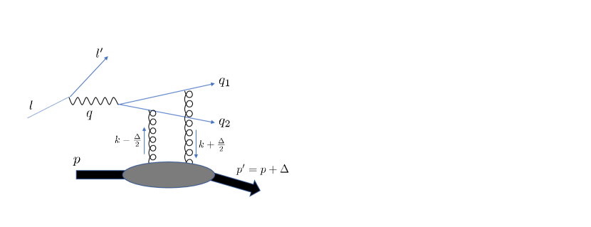
Figure 1: Diagrammatic interpretation of the nucleon’s gravitational form factor $D(|\vec{k}|)$. The wavy line denotes a graviton. Left: two vector meson (pion) exchanges at $\vec{k}=0$; Middle: $2^{++}$ and $0^{++}$ glueball exchanges when $|\vec{k}|\lesssim 1$ GeV; Right: two gluon exchanges in the perturbative high-$|\vec{k}|$ ($\gg 1$ GeV) region.

The connection between the D-term and glueballs has been recently emphasized by Mamo and Zahed using a bottom-up AdS₅/QCD₄ model [36, 18]. As we commented at the end of Section 5, in their calculation the D-term results from a cancellation between the transverse-traceless (TT) graviton and dilaton exchanges in AdS₅ (in other words, between the first and second lines in (2.5)). They argue that, due to the degeneracy of the $2^{++}$ and $0^{++}$ glueball masses, the cancellation is complete (meaning $D=0$) in the large-$N_{c}$ limit. They further argue that the D-term becomes nonzero only after including $1/N_{c}$ corrections, suggesting that the large-$N_{c}$ counting argument [2]

$$D\sim O(N_{c}^{2}),$$ (6.1)

does not hold. In contrast, in our AdS₇/CFT₆/QCD₄ calculation, the contributions from the $2^{++}$ and $0^{++}$ T₄ glueballs add up (see (5.71), (5.73)), after which their distinction becomes immaterial. Moreover, the value $D(k=0)$ can be calculated ‘classically’ as in Section 4 without any reference to glueballs. Our result is consistent with the large-$N_{c}$ counting since

$$D\sim\kappa M\sim O(N_{c}^{2}).$$ (6.2)

($M_{KK}\sim O(N_{c}^{0})$ since it is related to the $\rho$-meson mass.) Interestingly, however, the actual numerical value calculated in Section 4 is small due to a cancellation between the iso-singlet and iso-vector contributions.

In conclusion, we have demonstrated that our model of QCD offers a novel holographic framework to calculate the nucleon D-term and possibly other gravitational form factors, with a vivid physical interpretation in terms of meson and glueball exchanges. There are a number of avenues for improvement and generalization. First, the quantization of the collective coordinates should be implemented. It is known that the quantization brings in uncertainties in baryon masses associated with the zero-point (vacuum) energy of harmonic oscillators [30]. We expect that the D-term, being a nonforward matrix element, is less affected by this problem. However, without quantization, the spin-1/2 nature of the nucleon is lost, and one cannot talk about the $B$-form factor (2.2). Second, in order to calculate $D(k)$ for nonvanishing values of $k$, it is desired to convolute a more accurate soliton configuration in the entire space $0<|z|<\infty$ obtained numerically (see e.g., [43, 44, 45]) with the graviton propagator to incorporate the contributions from the glueballs. This is crucial, in particular, for the calculation of the ‘mechanical radius’ [2]

$$\langle r^{2}\rangle\equiv\frac{6D(0)}{\int_{0}^{\infty}dk^{2}D(k^{2})}.$$ (6.3)

Since the entire region in $k$ is involved, a proper evaluation of the mechanical radius must include the glueball degrees of freedom. The calculation is significantly more complex than that of the electromagnetic form factors and the associated ‘charge radius’ in this model [32] which only requires the knowledge of the asymptotic behavior $z\to\infty$ of the bulk gauge fields. There are other interesting directions such as the effect of finite quark masses (finite pion mass) and generalizations to mesons and excited baryons [70], and perhaps even to atomic nuclei [71]. We hope to address these issues in future.

References

• [1] P. A. Zyla et al. [Particle Data Group], “Review of Particle Physics,” PTEP 2020 (2020) no.8, 083C01 doi:10.1093/ptep/ptaa104
• [2] M. V. Polyakov and P. Schweitzer, “Forces inside hadrons: pressure, surface tension, mechanical radius, and all that,” Int. J. Mod. Phys. A 33 (2018) no.26, 1830025 doi:10.1142/S0217751X18300259 [arXiv:1805.06596 [hep-ph]].
• [3] I. Y. Kobzarev and L. B. Okun, “GRAVITATIONAL INTERACTION OF FERMIONS,” Zh. Eksp. Teor. Fiz. 43 (1962), 1904-1909
• [4] H. Pagels, “Energy-Momentum Structure Form Factors of Particles,” Phys. Rev. 144 (1966), 1250-1260 doi:10.1103/PhysRev.144.1250
• [5] R. Abdul Khalek, A. Accardi, J. Adam, D. Adamiak, W. Akers, M. Albaladejo, A. Al-bataineh, M. G. Alexeev, F. Ameli and P. Antonioli, et al. “Science Requirements and Detector Concepts for the Electron-Ion Collider: EIC Yellow Report,” [arXiv:2103.05419 [physics.ins-det]].
• [6] Y. Hatta, Y. V. Kovchegov, C. Marquet, A. Prokudin, E. Aschenauer, H. Avakian, A. Bacchetta, D. Boer, G. A. Chirilli and A. Dumitru, et al. “Proceedings, Probing Nucleons and Nuclei in High Energy Collisions: Dedicated to the Physics of the Electron Ion Collider: Seattle (WA), United States, October 1 - November 16, 2018,” doi:10.1142/11684 [arXiv:2002.12333 [hep-ph]].
• [7] D. P. Anderle, V. Bertone, X. Cao, L. Chang, N. Chang, G. Chen, X. Chen, Z. Chen, Z. Cui and L. Dai, et al. “Electron-Ion Collider in China,” [arXiv:2102.09222 [nucl-ex]].
• [8] V. D. Burkert, L. Elouadrhiri and F. X. Girod, “The pressure distribution inside the proton,” Nature 557 (2018) no.7705, 396-399 doi:10.1038/s41586-018-0060-z
• [9] O. V. Teryaev, “Analytic properties of hard exclusive amplitudes,” [arXiv:hep-ph/0510031 [hep-ph]].
• [10] I. V. Anikin and O. V. Teryaev, Phys. Rev. D 76 (2007), 056007 doi:10.1103/PhysRevD.76.056007 [arXiv:0704.2185 [hep-ph]].
• [11] Y. Hatta and D. L. Yang, “Holographic $J/\psi$ production near threshold and the proton mass problem,” Phys. Rev. D 98 (2018) no.7, 074003 doi:10.1103/PhysRevD.98.074003 [arXiv:1808.02163 [hep-ph]].
• [12] Y. Hatta, A. Rajan and D. L. Yang, “Near threshold $J/\psi$ and $\Upsilon$ photoproduction at JLab and RHIC,” Phys. Rev. D 100 (2019) no.1, 014032 doi:10.1103/PhysRevD.100.014032 [arXiv:1906.00894 [hep-ph]].
• [13] R. Boussarie and Y. Hatta, “QCD analysis of near-threshold quarkonium leptoproduction at large photon virtualities,” Phys. Rev. D 101 (2020) no.11, 114004 doi:10.1103/PhysRevD.101.114004 [arXiv:2004.12715 [hep-ph]].
• [14] Y. Hatta and M. Strikman, “$\phi$-meson lepto-production near threshold and the strangeness $D$-term,” Phys. Lett. B 817 (2021), 136295 doi:10.1016/j.physletb.2021.136295 [arXiv:2102.12631 [hep-ph]].
• [15] Y. Guo, X. Ji and Y. Liu, “QCD Analysis of Near-Threshold Photon-Proton Production of Heavy Quarkonium,” Phys. Rev. D 103 (2021) no.9, 096010 doi:10.1103/PhysRevD.103.096010 [arXiv:2103.11506 [hep-ph]].
• [16] D. E. Kharzeev, “Mass radius of the proton,” Phys. Rev. D 104, no.5, 054015 (2021) doi:10.1103/PhysRevD.104.054015 [arXiv:2102.00110 [hep-ph]].
• [17] R. Wang, W. Kou, Y. P. Xie and X. Chen, “Extraction of the proton mass radius from the vector meson photoproductions near thresholds,” Phys. Rev. D 103, no.9, L091501 (2021) doi:10.1103/PhysRevD.103.L091501 [arXiv:2102.01610 [hep-ph]].
• [18] K. A. Mamo and I. Zahed, [arXiv:2204.08857 [hep-ph]].
• [19] K. A. Mamo and I. Zahed, “Diffractive photoproduction of $J/\psi$ and $\Upsilon$ using holographic QCD: gravitational form factors and GPD of gluons in the proton,” Phys. Rev. D 101 (2020) no.8, 086003 doi:10.1103/PhysRevD.101.086003 [arXiv:1910.04707 [hep-ph]].
• [20] M. L. Du, V. Baru, F. K. Guo, C. Hanhart, U. G. Meißner, A. Nefediev and I. Strakovsky, “Deciphering the mechanism of near-threshold $J/\psi$ photoproduction,” Eur. Phys. J. C 80 (2020) no.11, 1053 doi:10.1140/epjc/s10052-020-08620-5 [arXiv:2009.08345 [hep-ph]].
• [21] P. Sun, X. B. Tong and F. Yuan, “Perturbative QCD analysis of near threshold heavy quarkonium photoproduction at large momentum transfer,” Phys. Lett. B 822 (2021), 136655 doi:10.1016/j.physletb.2021.136655 [arXiv:2103.12047 [hep-ph]].
• [22] K. A. Mamo and I. Zahed, “Electroproduction of heavy vector mesons using holographic QCD: From near threshold to high energy regimes,” Phys. Rev. D 104 (2021) no.6, 066023 doi:10.1103/PhysRevD.104.066023 [arXiv:2106.00722 [hep-ph]].
• [23] P. Sun, X. B. Tong and F. Yuan, “Near Threshold Heavy Quarkonium Photoproduction at Large Momentum Transfer,” [arXiv:2111.07034 [hep-ph]].
• [24] D. A. Pefkou, D. C. Hackett and P. E. Shanahan, “Gluon gravitational structure of hadrons of different spin,” [arXiv:2107.10368 [hep-lat]].
• [25] M. V. Polyakov, “Generalized parton distributions and strong forces inside nucleons and nuclei,” Phys. Lett. B 555 (2003), 57-62 doi:10.1016/S0370-2693(03)00036-4 [arXiv:hep-ph/0210165 [hep-ph]].
• [26] T. Sakai and S. Sugimoto, “Low energy hadron physics in holographic QCD,” Prog. Theor. Phys. 113 (2005), 843-882 doi:10.1143/PTP.113.843 [arXiv:hep-th/0412141 [hep-th]].
• [27] T. Sakai and S. Sugimoto, “More on a holographic dual of QCD,” Prog. Theor. Phys. 114 (2005), 1083-1118 doi:10.1143/PTP.114.1083 [arXiv:hep-th/0507073 [hep-th]].
• [28] K. Nawa, H. Suganuma and T. Kojo, “Baryons in holographic QCD,” Phys. Rev. D 75 (2007), 086003 doi:10.1103/PhysRevD.75.086003 [arXiv:hep-th/0612187 [hep-th]].
• [29] D. K. Hong, M. Rho, H. U. Yee and P. Yi, “Chiral Dynamics of Baryons from String Theory,” Phys. Rev. D 76 (2007), 061901 doi:10.1103/PhysRevD.76.061901 [arXiv:hep-th/0701276 [hep-th]].
• [30] H. Hata, T. Sakai, S. Sugimoto and S. Yamato, “Baryons from instantons in holographic QCD,” Prog. Theor. Phys. 117 (2007), 1157 doi:10.1143/PTP.117.1157 [arXiv:hep-th/0701280 [hep-th]].
• [31] D. K. Hong, M. Rho, H. U. Yee and P. Yi, “Dynamics of baryons from string theory and vector dominance,” JHEP 09 (2007), 063 doi:10.1088/1126-6708/2007/09/063 [arXiv:0705.2632 [hep-th]].
• [32] K. Hashimoto, T. Sakai and S. Sugimoto, “Holographic Baryons: Static Properties and Form Factors from Gauge/String Duality,” Prog. Theor. Phys. 120 (2008), 1093-1137 doi:10.1143/PTP.120.1093 [arXiv:0806.3122 [hep-th]].
• [33] D. K. Hong, M. Rho, H. U. Yee and P. Yi, “Nucleon form-factors and hidden symmetry in holographic QCD,” Phys. Rev. D 77 (2008), 014030 doi:10.1103/PhysRevD.77.014030 [arXiv:0710.4615 [hep-ph]].
• [34] K. Y. Kim and I. Zahed, “Electromagnetic Baryon Form Factors from Holographic QCD,” JHEP 09 (2008), 007 doi:10.1088/1126-6708/2008/09/007 [arXiv:0807.0033 [hep-th]].
• [35] Z. Abidin and C. E. Carlson, “Nucleon electromagnetic and gravitational form factors from holography,” Phys. Rev. D 79 (2009), 115003 doi:10.1103/PhysRevD.79.115003 [arXiv:0903.4818 [hep-ph]].
• [36] K. A. Mamo and I. Zahed, “Nucleon mass radii and distribution: Holographic QCD, Lattice QCD and GlueX data,” Phys. Rev. D 103 (2021) no.9, 094010 doi:10.1103/PhysRevD.103.094010 [arXiv:2103.03186 [hep-ph]].
• [37] D. Chakrabarti, C. Mondal, A. Mukherjee, S. Nair and X. Zhao, “Gravitational form factors and mechanical properties of proton in a light-front quark-diquark model,” Phys. Rev. D 102 (2020), 113011 doi:10.1103/PhysRevD.102.113011 [arXiv:2010.04215 [hep-ph]].
• [38] K. Goeke, J. Grabis, J. Ossmann, M. V. Polyakov, P. Schweitzer, A. Silva and D. Urbano, “Nucleon form-factors of the energy momentum tensor in the chiral quark-soliton model,” Phys. Rev. D 75 (2007), 094021 doi:10.1103/PhysRevD.75.094021 [arXiv:hep-ph/0702030 [hep-ph]].
• [39] C. Cebulla, K. Goeke, J. Ossmann and P. Schweitzer, “The Nucleon form-factors of the energy momentum tensor in the Skyrme model,” Nucl. Phys. A 794 (2007), 87-114 doi:10.1016/j.nuclphysa.2007.08.004 [arXiv:hep-ph/0703025 [hep-ph]].
• [40] I. A. Perevalova, M. V. Polyakov and P. Schweitzer, “On LHCb pentaquarks as a baryon-$\psi$(2S) bound state: prediction of isospin-$\frac{3}{2}$ pentaquarks with hidden charm,” Phys. Rev. D 94 (2016) no.5, 054024 doi:10.1103/PhysRevD.94.054024 [arXiv:1607.07008 [hep-ph]].
• [41] J. Y. Kim and B. D. Sun, “Gravitational form factors of a baryon with spin-3/2,” Eur. Phys. J. C 81 (2021) no.1, 85 doi:10.1140/epjc/s10052-021-08852-z [arXiv:2011.00292 [hep-ph]].
• [42] A. A. Belavin, A. M. Polyakov, A. S. Schwartz and Y. S. Tyupkin, “Pseudoparticle Solutions of the Yang-Mills Equations,” Phys. Lett. B 59 (1975), 85-87 doi:10.1016/0370-2693(75)90163-X
• [43] S. Bolognesi and P. Sutcliffe, “The Sakai-Sugimoto soliton,” JHEP 01 (2014), 078 doi:10.1007/JHEP01(2014)078 [arXiv:1309.1396 [hep-th]].
• [44] M. Rozali, J. B. Stang and M. van Raamsdonk, “Holographic Baryons from Oblate Instantons,” JHEP 02 (2014), 044 doi:10.1007/JHEP02(2014)044 [arXiv:1309.7037 [hep-th]].
• [45] H. Suganuma and K. Hori, “Topological Objects in Holographic QCD,” Phys. Scripta 95 (2020) no.7, 074014 doi:10.1088/1402-4896/ab986c [arXiv:2003.07127 [hep-th]].
• [46] A. Karch, A. O’Bannon and E. Thompson, “The Stress-Energy Tensor of Flavor Fields from AdS/CFT,” JHEP 04 (2009), 021 doi:10.1088/1126-6708/2009/04/021 [arXiv:0812.3629 [hep-th]].
• [47] G. S. Adkins and C. R. Nappi, “Stabilization of Chiral Solitons via Vector Mesons,” Phys. Lett. B 137 (1984), 251-256 doi:10.1016/0370-2693(84)90239-9
• [48] J. P. Boyd, “Chebyshev and Fourier Spectral Methods,” Courier Corporation, 2001.
• [49] P. Virtanen et al. “SciPy 1.0–Fundamental Algorithms for Scientific Computing in Python,” Nature Meth. 17 (2020), 261 doi:10.1038/s41592-019-0686-2 [arXiv:1907.10121 [cs.MS]].
• [50] Eigen, http://eigen.tuxfamily.org.
• [51] Boost libraries, https://www.boost.org.
• [52] A. Metz, B. Pasquini and S. Rodini, Phys. Lett. B 820 (2021), 136501 doi:10.1016/j.physletb.2021.136501 [arXiv:2104.04207 [hep-ph]].
• [53] X. Ji and Y. Liu, “Momentum-Current Gravitational Multipoles of Hadrons,” [arXiv:2110.14781 [hep-ph]].
• [54] V. Balasubramanian and P. Kraus, Commun. Math. Phys. 208 (1999), 413-428 doi:10.1007/s002200050764 [arXiv:hep-th/9902121 [hep-th]].
• [55] S. de Haro, S. N. Solodukhin and K. Skenderis, “Holographic reconstruction of space-time and renormalization in the AdS / CFT correspondence,” Commun. Math. Phys. 217 (2001), 595-622 doi:10.1007/s002200100381 [arXiv:hep-th/0002230 [hep-th]].
• [56] I. Kanitscheider, K. Skenderis and M. Taylor, “Precision holography for non-conformal branes,” JHEP 09 (2008), 094 doi:10.1088/1126-6708/2008/09/094 [arXiv:0807.3324 [hep-th]].
• [57] E. Witten, “Baryons and branes in anti-de Sitter space,” JHEP 9807, 006 (1998) doi:10.1088/1126-6708/1998/07/006 [hep-th/9805112].
• [58] N. R. Constable and R. C. Myers, “Spin two glueballs, positive energy theorems and the AdS / CFT correspondence,” JHEP 10 (1999), 037 doi:10.1088/1126-6708/1999/10/037 [arXiv:hep-th/9908175 [hep-th]].
• [59] R. C. Brower, S. D. Mathur and C. I. Tan, “Glueball spectrum for QCD from AdS supergravity duality,” Nucl. Phys. B 587 (2000), 249-276 doi:10.1016/S0550-3213(00)00435-1 [arXiv:hep-th/0003115 [hep-th]].
• [60] A. Hashimoto and Y. Oz, “Aspects of QCD dynamics from string theory,” Nucl. Phys. B 548 (1999), 167-179 doi:10.1016/S0550-3213(99)00120-0 [arXiv:hep-th/9809106 [hep-th]].
• [61] K. Hashimoto, C. I. Tan and S. Terashima, “Glueball decay in holographic QCD,” Phys. Rev. D 77 (2008), 086001 doi:10.1103/PhysRevD.77.086001 [arXiv:0709.2208 [hep-th]].
• [62] F. Brünner, D. Parganlija and A. Rebhan, “Glueball Decay Rates in the Witten-Sakai-Sugimoto Model,” Phys. Rev. D 91 (2015) no.10, 106002 [erratum: Phys. Rev. D 93 (2016) no.10, 109903] doi:10.1103/PhysRevD.91.106002 [arXiv:1501.07906 [hep-ph]].
• [63] B. A. Burrington, V. S. Kaplunovsky and J. Sonnenschein, “Localized Backreacted Flavor Branes in Holographic QCD,” JHEP 02 (2008), 001 doi:10.1088/1126-6708/2008/02/001 [arXiv:0708.1234 [hep-th]].
• [64] J. J. Friess, S. S. Gubser, G. Michalogiorgakis and S. S. Pufu, “The Stress tensor of a quark moving through N=4 thermal plasma,” Phys. Rev. D 75 (2007), 106003 doi:10.1103/PhysRevD.75.106003 [arXiv:hep-th/0607022 [hep-th]].
• [65] K. Tanaka, “Operator relations for gravitational form factors of a spin-0 hadron,” Phys. Rev. D 98 (2018) no.3, 034009 doi:10.1103/PhysRevD.98.034009 [arXiv:1806.10591 [hep-ph]].
• [66] X. B. Tong, J. P. Ma and F. Yuan, “Gluon gravitational form factors at large momentum transfer,” Phys. Lett. B 823 (2021), 136751 doi:10.1016/j.physletb.2021.136751 [arXiv:2101.02395 [hep-ph]].
• [67] X. B. Tong, J. P. Ma and F. Yuan, “Perturbative Calculations of Gravitational Form Factors at Large Momentum Transfer,” [arXiv:2203.13493 [hep-ph]].
• [68] W. Mueck and K. S. Viswanathan, “Conformal field theory correlators from classical scalar field theory on AdS(d+1),” Phys. Rev. D 58 (1998), 041901 doi:10.1103/PhysRevD.58.041901 [arXiv:hep-th/9804035 [hep-th]].
• [69] S. S. Gubser and S. S. Pufu, “Master field treatment of metric perturbations sourced by the trailing string,” Nucl. Phys. B 790 (2008), 42-71 doi:10.1016/j.nuclphysb.2007.08.015 [arXiv:hep-th/0703090 [hep-th]].
• [70] Y. Hayashi, T. Ogino, T. Sakai and S. Sugimoto, “Stringy excited baryons in holographic quantum chromodynamics,” PTEP 2020 (2020) no.5, 053B04 doi:10.1093/ptep/ptaa045 [arXiv:2001.01461 [hep-th]].
• [71] K. Hashimoto, Y. Matsuo and T. Morita, “Nuclear states and spectra in holographic QCD,” JHEP 12 (2019), 001 doi:10.1007/JHEP12(2019)001 [arXiv:1902.07444 [hep-th]].