Physics Informed Neural Fields for Smoke Reconstruction with Sparse Data
Abstract.
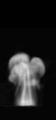
High-fidelity reconstruction of dynamic fluids from sparse multiview RGB videos remains a formidable challenge, due to the complexity of the underlying physics as well as the severe occlusion and complex lighting in the captured data. Existing solutions either assume knowledge of obstacles and lighting, or only focus on simple fluid scenes without obstacles or complex lighting, and thus are unsuitable for real-world scenes with unknown lighting conditions or arbitrary obstacles. We present the first method to reconstruct dynamic fluid phenomena by leveraging the governing physics (ie, Navier -Stokes equations) in an end-to-end optimization from a mere set of sparse video frames without taking lighting conditions, geometry information, or boundary conditions as input. Our method provides a continuous spatio-temporal scene representation using neural networks as the ansatz of density and velocity solution functions for fluids as well as the radiance field for static objects. With a hybrid architecture that separates static and dynamic contents apart, fluid interactions with static obstacles are reconstructed for the first time without additional geometry input or human labeling. By augmenting time-varying neural radiance fields with physics-informed deep learning, our method benefits from the supervision of images and physical priors. To achieve robust optimization from sparse input views, we introduced a layer-by-layer growing strategy to progressively increase the network capacity of the resulting neural representation. Using our progressively growing models with a newly proposed regularization term, we manage to disentangle the density-color ambiguity in radiance fields without overfitting. A pretrained density-to-velocity fluid model is leveraged in addition as the data prior to avoid suboptimal velocity solutions which underestimate vorticity but trivially fulfill physical equations. Our method exhibits high-quality results with relaxed constraints and strong flexibility on a representative set of synthetic and real flow captures. Code and sample tests are at https://people.mpi-inf.mpg.de/~mchu/projects/PI-NeRF/.
\begin{overpic}[height=90.0pt]{fig/teaser/r1.jpg}
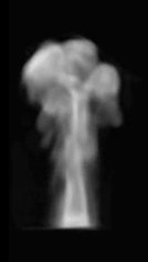
\put(3.0,182.0){{\color[rgb]{1,1,0.2}\definecolor[named]{pgfstrokecolor}{rgb}{1,1,0.2}\pgfsys@color@cmyk@stroke{0}{0}{0.8}{0}\pgfsys@color@cmyk@fill{0}{0}{0.8}{0} - Synthetic plume -}}
\put(5.0,102.0){{\color[rgb]{1,1,1}\definecolor[named]{pgfstrokecolor}{rgb}{1,1,1}\pgfsys@color@gray@stroke{1}\pgfsys@color@gray@fill{1} \footnotesize{Novel view}}}
\put(8.0,92.0){{\color[rgb]{1,1,1}\definecolor[named]{pgfstrokecolor}{rgb}{1,1,1}\pgfsys@color@gray@stroke{1}\pgfsys@color@gray@fill{1} \footnotesize{rendering}}}
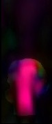
\end{overpic}\begin{overpic}[height=92.0pt]{fig/teaser/r1v.jpg}
\put(8.0,102.0){{\color[rgb]{1,1,1}\definecolor[named]{pgfstrokecolor}{rgb}{1,1,1}\pgfsys@color@gray@stroke{1}\pgfsys@color@gray@fill{1} \footnotesize{Velocity and vorticity}}}
\put(16.0,92.0){{\color[rgb]{1,1,1}\definecolor[named]{pgfstrokecolor}{rgb}{1,1,1}\pgfsys@color@gray@stroke{1}\pgfsys@color@gray@fill{1} \footnotesize{visualizations}}}
\put(-48.0,2.0){{\color[rgb]{1,1,0.2}\definecolor[named]{pgfstrokecolor}{rgb}{1,1,0.2}\pgfsys@color@cmyk@stroke{0}{0}{0.8}{0}\pgfsys@color@cmyk@fill{0}{0}{0.8}{0} - Real capture -}}
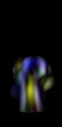
\end{overpic}\begin{overpic}[height=92.0pt]{fig/teaser/r2.jpg}
\put(20.0,102.0){{\color[rgb]{1,1,1}\definecolor[named]{pgfstrokecolor}{rgb}{1,1,1}\pgfsys@color@gray@stroke{1}\pgfsys@color@gray@fill{1} \footnotesize{Rendering,
velocity and vorticity at a later time step}}}
\end{overpic} \begin{overpic}[height=189.0pt]{fig/teaser/car.jpg}
\put(2.0,2.0){{\color[rgb]{1,1,0.2}\definecolor[named]{pgfstrokecolor}{rgb}{1,1,0.2}\pgfsys@color@cmyk@stroke{0}{0}{0.8}{0}\pgfsys@color@cmyk@fill{0}{0}{0.8}{0} - Hybrid Scene -}}
\put(38.0,28.0){{\color[rgb]{1,1,1}\definecolor[named]{pgfstrokecolor}{rgb}{1,1,1}\pgfsys@color@gray@stroke{1}\pgfsys@color@gray@fill{1} \footnotesize{Rendering of the dynamic part}}}
\put(42.0,60.0){{\color[rgb]{1,1,1}\definecolor[named]{pgfstrokecolor}{rgb}{1,1,1}\pgfsys@color@gray@stroke{1}\pgfsys@color@gray@fill{1} \footnotesize{Rendering of the static part}}}
\put(56.0,96.0){{\color[rgb]{1,1,1}\definecolor[named]{pgfstrokecolor}{rgb}{1,1,1}\pgfsys@color@gray@stroke{1}\pgfsys@color@gray@fill{1} \footnotesize{Rendering of both}}}
\end{overpic}
\begin{overpic}[height=189.0pt]{fig/teaser/car.jpg}
\put(2.0,2.0){{\color[rgb]{1,1,0.2}\definecolor[named]{pgfstrokecolor}{rgb}{1,1,0.2}\pgfsys@color@cmyk@stroke{0}{0}{0.8}{0}\pgfsys@color@cmyk@fill{0}{0}{0.8}{0} - Hybrid Scene -}}
\put(38.0,28.0){{\color[rgb]{1,1,1}\definecolor[named]{pgfstrokecolor}{rgb}{1,1,1}\pgfsys@color@gray@stroke{1}\pgfsys@color@gray@fill{1} \footnotesize{Rendering of the dynamic part}}}
\put(42.0,60.0){{\color[rgb]{1,1,1}\definecolor[named]{pgfstrokecolor}{rgb}{1,1,1}\pgfsys@color@gray@stroke{1}\pgfsys@color@gray@fill{1} \footnotesize{Rendering of the static part}}}
\put(56.0,96.0){{\color[rgb]{1,1,1}\definecolor[named]{pgfstrokecolor}{rgb}{1,1,1}\pgfsys@color@gray@stroke{1}\pgfsys@color@gray@fill{1} \footnotesize{Rendering of both}}}
\end{overpic}
1. Introduction
Obeying general laws of physics, fluid phenomena are ubiquitous and various. The understanding of fluids benefit a wide range of activities including weather forecasting [Bauer et al., 2015], vehicle manufacturing [Bushnell and Moore, 1991], medicine metabolism [Shi et al., 2010], and visual effects [Kim et al., 2008; Xie et al., 2018]. In studying the fluid behaviors, one of the core tasks is to estimate the invisible velocity. In general, velocity can be obtained either by solving physical equations with numerical solvers [Bridson, 2015] or by measuring experimentally, e.g. particle image velocimetry (PIV) [Elsinga et al., 2006], both with different pros and cons.
With the progress in hardware and algorithms, numerical solvers achieve high accuracy in “forward” fluid simulation tasks, e.g. analyzing canonical flows, where experienced engineers are able to provide a full set of initial and boundary conditions, etc. However, due to partially available initial conditions, common users cannot easily apply them in an “inverse” manner to handle particular fluid phenomena in real life, e.g. steam rising up from a teapot. Experimental techniques, including PIV, allow users to estimate real-life fluid behavior. In these works [Grant, 1997; Xiong et al., 2017], the scope is limited to simple scenes with fluid as the main objective. By estimating the volumetric distribution of a passive scalar, e.g. tracer particles, colorful dye, or smoke, from image modalities, the underlying motion is then inferred from the transport and physical equations. As PIV methods require specialized lab settings, there has been growing interest in fluid reconstructions from RGB images [Gregson et al., 2014; Franz et al., 2021]. Despite improvements in reconstruction quality and reduction of hardware, existing approaches are still vulnerable to scenes with unknown illumination or occluding obstacles.
We aim to overcome these difficulties, handle fluid scenes with unknown lighting and arbitrary obstacles, and advance the goal of capturing fluids in the wild. In addition to reducing the constraints for fluid capture, being able to handle fluid scenes with obstacles is an important step towards analyzing fluid-obstacle interactions.
Based on recent progress in view synthesis using neural radiance fields (NeRF) [Lombardi et al., 2019; Mildenhall et al., 2020], we first augment the spatial scene representation in the time dimension and learn a time-varying neural radiance field. Taking RGB videos of a scene with dynamic fluid as input, the time-varying NeRF learns to encode a spatiotemporal radiance field with a Multi-Layered Perceptron (MLPs). Originally proposed for static scenes, NeRF uses differentiable rendering to gather information from multiview images with different camera poses. Correspondingly, in our case, it is important to apply differentiable physics to unify information from video frames at different time steps as a dynamic NeRF. Thus, we propose to use physics-informed deep learning technologies [Raissi et al., 2020] and use another MLP to represent the continuous spatio-temporal velocity field. With jointly applied differentiable rendering and physics models, we manage to learn the continuous spatiotemporal radiance and velocity fields in a dynamic scene and supervise them using image sequences and physical laws end to end. Similar to Physics-Informed Neural Networks (PINN), partial differential equations (PDE) are calculated using the exact, mesh-free derivatives of the velocity model via auto-differentiation without discretization.
Through a seamless intertwining of NeRF and PINN, our method learns physics-informed neural fluid fields from image sequences end to end. It is unrestrained by lighting conditions, geometry information, or the initial and boundary conditions, and is therefore suitable for hybrid scenes with obstacles. Our method also face the same issues of PINN methods: the training task is challenging due to the complex non-linear optimization landscape shaped by PDE constraints. Specifically, in fluid reconstruction, this issue tends to manifest itself as underestimated vorticity and density overfitting to given views. While overfitting problems are usually handled with regularization terms, more data, or model-based supervision, we propose to use a regularization term on the density and a published pre-trained velocity model [Chu et al., 2021] to reduce the vorticity underestimation. While both Neural Volumes [Lombardi et al., 2019] and the static NeRF have to use a large number of images with different camera poses to properly disentangle the radiance color and opacity, we show that our density regularization term helps to effectively disentangle this color-density ambiguity of the radiance field, which eventually allows us to work with sparse camera views. The general pipeline of our algorithm is illustrated in Fig. 2.
To summarize, our work makes the following contributions:
-
•
We propose the first method for reconstructing dynamic fluids with high quality from sparse multi-view RGB videos, without access to any lighting and geometry information.
-
•
We introduce a hybrid representation for dynamic fluid scenes interacting with static obstacles. It allows automatic separation of dynamic and static components without any human labelling, which is previously not possible.
-
•
We propose comprehensive supervision using images, physical priors (i.e., Navier-Stokes equations), as well as a pre-trained fluid model as data prior to prevent sub-optimal solutions with underestimated vorticity.
-
•
We propose a progressively growing model with a new regularization term to penalize “ghost density”, an artifact caused by color-density ambiguity.Together, overfitting to sparse given views is avoided.
With these, our method relaxes the requirements of fluid reconstruction, enables the capture of fluid behavior with obstacles, and achieves state-of-the-art results in both synthetic and real scenes.
2. Related Work
We summarize related work in fluid reconstruction, physics-informed deep learning, and neural scene representations.
2.1. Fluid Reconstruction Methods
Several approaches have been proposed to reconstruct fluids from observations of visible light measurements. There are established methods that use active sensing with specialized hardware and lighting setups [Atcheson et al., 2009; Gu et al., 2013; Ji et al., 2013] and particle imaging velocimetry (PIV) [Grant, 1997; Elsinga et al., 2006; Xiong et al., 2017] injecting passive markers into fluid flows. PIV methods usually require specialized setups for particles, lighting, and capture. Many flow phenomena, e.g. smoke and fire, have visible elements which can easily be recorded. In the following, we focus on fluid reconstruction using RGB images to alleviate the need for specialized setups. Early work [Gregson et al., 2014] uses linear image formation to extract passive quantities from simple RGB images and reconstruct fluids with physical priors. Extending this direction, ScalarFlow [Eckert et al., 2019] reconstructs real-world smoke plumes from sparse views and Zang et al. [2020] use interpolated views as further constraints. Instead of using linear image formation, the Global Transport method [Franz et al., 2021] uses differentiable rendering to allow end-to-end optimization. Qiu et al. [2021] train convolutional networks end-to-end to estimate flow from sequences of orthogonal views. These methods either require known lighting conditions or ignore lighting altogether. Most related work reconstruct velocity on discrete grids, while we employ MLPs as an ansatz for fluid and present continuous velocity fields.
2.2. Physics Informed Deep Learning
Physics-informed deep learning respects physical equations governing a certain problem, e.g. Partial Differential Equations (PDE), by coupling them into the learning process. These methods [Pakravan et al., 2021; Raissi et al., 2019] have emerged as essential tools for various challenging forward and inverse problems. By coupling differentiable numerical solvers into training, physically plausible solutions can be obtained for dynamic problems, e.g. cloths [Geng et al., 2020] and fluids [Um et al., 2020; Gibou et al., 2019]. Besides using discretized numerical solvers, PINN [Raissi et al., 2019] proposes employing MLPs as continuous network surrogates for dynamics. Early MLP-based models [Lagaris et al., 1998; He et al., 2000; Mai-Duy and Tran-Cong, 2003] use a small number of hidden layers and hyperbolic tangent or sigmoid nonlinearities. The network capacity is restricted. Current approaches [Sirignano and Spiliopoulos, 2018; Raissi et al., 2020; Berg and Nyström, 2018] advanced on equation sophistication and dimensionality by capitalizing on new optimization frameworks and autodifferentiation for training MLP-based networks. Recent studies [Sitzmann et al., 2020; Tancik et al., 2020] have demonstrated that the commonly used MLPs struggle with high-frequency information and propose new periodic activation functions to represent complex natural signals and their derivatives.
2.3. Neural Representations
In scene representations, neural representations have recently been widespread for their expressiveness and compactness.
Neural intermediate representations
To synthesize novel views of a 3D scene, multi-plane images [Zhou et al., 2018; Mildenhall et al., 2019; Srinivasan et al., 2019], multi-sphere images [Broxton et al., 2020] and proxy geometries [Zhang et al., 2021; Philip et al., 2019] are proposed to build intermediate neural representations from multiple views. Novel views can be rendered with learned representations in interpolation or extrapolation manners. Eslami et al. [2018] propose to learn a neural embedding from observed images of a scene and infer unseen novel views. Granskog et al. [2020] further partition and compress the neural embedding into concise components which enables compositional rendering.
Neural explicit representations
By leveraging inverse rendering, classic 3D representations have been adapted to neural versions. Yifan et al. [2019] introduce differentiable surface splatting to enable point-cloud-based geometry processing from images. DeepVoxels [Sitzmann et al., 2019a] learns a 3D feature representation and stores features in a voxel grid for novel view synthesis. Neural Volumes [Lombardi et al., 2019] encodes objects in a voxel grid and learns an inverse mapping to decode voxelized radiance. These grid-based discretization suffers from resolution limitations.
Neural implicit representations
To avoid the resolution limitation of discretization, implicit 3D representations, including signed distance functions (SDF) [Park et al., 2019; Chabra et al., 2020], unsigned distance functions [Chibane et al., 2020], and occupancy fields [Chen and Zhang, 2019; Peng et al., 2020], are parameterized with neural networks to represent 3D shapes. Furthermore, these continuous representations are generalized to coordinate-based networks. For 3D shapes with textured surfaces, scene representation networks [Sitzmann et al., 2019b] learn SDFs and texture color for each coordinate. Niemeyer et al. [2020] derive implicit gradients to enable optimization and learn the surface radiance. Instead of SDF, PIfu [Saito et al., 2019] proposes to predict surface occupancy and color for coordinates. Different from scene representations based on opaque surfaces, NeRF [Mildenhall et al., 2020] represents scenes as implicit volumes and trains the coordinate-based networks to approximate continuous volumetric radiance fields. After training, novel views are rendered by ray marching. Many extensions have been proposed for fast rendering [Liu et al., 2020; Reiser et al., 2021; Yu et al., 2021; Garbin et al., 2021; Hedman et al., 2021], geometry reconstruction [Yariv et al., 2020; Oechsle et al., 2021; Yariv et al., 2021; Wang et al., 2021], generative image synthesis [Schwarz et al., 2020; Niemeyer and Geiger, 2021; Gu et al., 2021], reflectance for opaque surfaces [Srinivasan et al., 2021], and participating media reconstruction [Zheng et al., 2021].
2.4. Neural Representations for Dynamic Scenes
As the above representations apply mainly to static scenes, there has been a steady effort targeting representations for dynamic scenes. Neural Volumes [Lombardi et al., 2019] and its follow-up works [Wang et al., 2020; Lombardi et al., 2021; Raj et al., 2021] employ an encoder-decoder to transform input images to a volume representation, followed by differentiable ray-marching. Some works [Tretschk et al., 2021; Park et al., 2020; Li et al., 2020; Park et al., 2021] design a dedicated deformation network to model the dense 3D motions of points between adjacent frames. Xian et al. [2020] model dynamic scenes as 4D space-time irradiance fields. Several works focus on human body rendering. Gafni et al. [2020] condition NeRF on face pose to represent a 4D facial avatar. Neural Body [Peng et al., 2021b] uses a SMPL model as a 3D proxy and attaches learnable features on each SMPL mesh vertices as anchors to connect spaces across difficult frames. Su et al. [2021] present an articulated NeRF based on a human skeleton for refining human pose estimation. Some works [Liu et al., 2021; Peng et al., 2021a; Chen et al., 2021] propose a geometry-guided deformable NeRF method for warping the space in different poses to a shared canonical space with a SMPL model as a 3D proxy. Neural Actor [Liu et al., 2021] learns pose-dependent deformation and appearance to model dynamic effects. Neural Human Performer [Kwon et al., 2021] proposes a generalizable NeRF based on a SMPL model with a temporal transformer and a multi-view transformer for new pose and appearance synthesis. In contrast, we focus on modeling the dynamic fluid with a new neural representation incorporated with physics-based constraints, which has not received much attention yet.
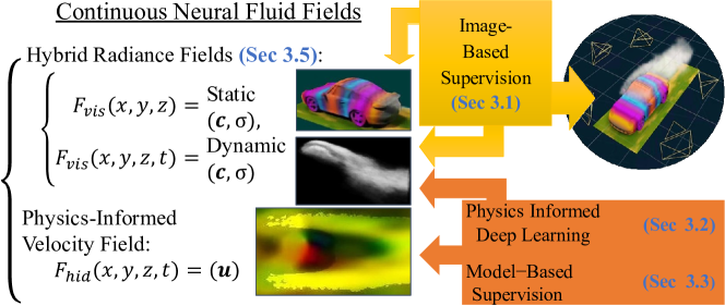
3. Neural Scene Representation For Fluids
Based on the universal approximation theorem, our method uses neural networks to represent a fluid scene in space and time. Mathematically, we use two MLP-based networks,
| (1) |
|
to approximate the continuous functions of the radiance field and velocity field, respectively. The input, , is the coordinate of a 4D location in space and time, the radiance output of contains the emitted color and the optical density . The velocity output of describes the 3D motion vector at that point and time. “hid” stands for the word “hidden”, since the velocity field is not directly observed. As a representation for fluid scenes, the radiance field provides us useful information about the lighting condition, object geometry, and the density distribution of the passive scalar in the scene. Meanwhile the velocity field describes the invisible dynamics which is important for further analysis of pressure or body forces for fluid mechanics. While it is possible to supervise directly using video sequences based on differentiable volumetric rendering, has to be trained indirectly from the density distribution of the passive scalar via physics equations. Note that physics equations are associated with mass density , which can be considered as being proportional to the optical density according to the Beer–Lambert law.
In the following, we describe the image-based supervision of in Sec. 3.1 and the physical equation-based supervision of in Sec. 3.2. Facing the highly non-linear and challenging optimization landscape formed by PDEs, we propose a model-based supervision in Sec. 3.3 to avoid sub-optimal solutions of with underestimated vorticity. In order to obtain a valid density distribution which will determine the best possible accuracy of , we propose to tackle the color-density ambiguity (Sec. 3.4) and disentangle the fluid and obstacle density (Sec. 3.5), respectively.
3.1. Image-Based Radiance Estimation
Briefly summarized, the static NeRF [Mildenhall et al., 2020] learns a static neural radiance field with a set of posed images though volumetric rendering. Here, is the coordinate of a position in 3D space and (, ) defines a ray direction as a 3D Cartesian unit vector . Considering the pixel of image , point samples are queried along the camera ray , where denotes the parametric distance. The color of the pixel is approximated with the numerical quadrature rule:
| (2) |
|
To sample rays efficiently with adaptive ray step , NeRF simultaneously optimizes two MLPs, a “coarse” one as a probability density function for importance sampling and a “fine” one as the target radiance field being sampled. Their parameters are then optimized with the following objective functions:
| (3) |
|
where is the reference color of pixel in image , and and are the color rendered by the coarse and fine models, respectively. Based on the ray casting based rendering algorithm, NeRF establishes the connection between 2D images and 3D geometry, supporting both solid objects as well as volumetric media.
In order to deal with dynamic scenes of fluid and explore the temporal evolution, we perform the following adaptations. First, we extend the static NeRF model with time as input. Second, we assume that the dynamic scene to be reconstructed only consists of Lambertian surfaces and media with isotropic scattering. Therefore, we remove the input and for simplicity. Finally, we use the MLP with periodic activation functions proposed in SIREN [Sitzmann et al., 2020] instead of ReLU-based MLPs with positional encoding strategies in order to model the continuous derivatives better. Same as the original NeRF, the quadrature rule is used for volumetric rendering and two models are trained as hierarchical volume sampling. Besides the loss in Eq. 3, we include a VGG-based perceptual loss term as proposed in previous work on image and video synthesis [Ledig et al., 2017; Chu et al., 2020]. Since it is time-consuming to render all pixels of a given image using the model, we randomly crop square patches from images with varying strides. In this way, only small image patches in resolution of are rendered during the training and we get VGG features at different scales. The VGG feature distances are measured using cosine similarity by:
| (4) |
|
As shown in Fig. 3, supervising the radiance fields with and VGG feature losses together helps to capture detailed structures better.
With these changes, we get a time-varying NeRF model based on SIREN layers: . It models the continuous functions of density and color and their derivatives in the space and time. Continuous derivative is necessary for learning the temporal evolution, which will be explained in the following section.
3.2. Physics-Informed Velocity Estimation
Recent approaches [Raissi et al., 2019, 2020] demonstrate that deep-learning models can be trained as data-driven solutions of physical problems via optimizing the governing PDEs, which are known as PINN. A distinctive feature shared by these studies is to use the continuous and mesh-free derivatives computed with auto-differentiation. For fluid dynamics, Raissi et al. [2020] train neural networks, , as the ansatz of the underlying solution functions. They propose to supervise the network using a ground-truth spatio-temporal dataset describing the distribution of the passive scalar with discrete data pairs . The aforementioned auto-differentiation is used to optimize the transport equation: , as well as the Navier-Stokes equations:
| (5) |
|
Without requiring boundary conditions as input, this method can handle fluid taking place in arbitrarily complex spacial domains. High accuracy of velocity and pressure can be achieved with a shallow MLP when physical parameters, e.g. kinematic viscosity , are given and the density is densely sampled from exact solutions.
Based on the PINN technology, we propose to learn a velocity network, , while training the radiance fields network mentioned in Sec. 3.1. Same as in , consists of SIREN layers [Sitzmann et al., 2020] with a principled initialization scheme, which allows for training deeper networks. Compared to the learning from ground-truth data [Raissi et al., 2020], we are facing a tougher learning task with more ambiguity since the density distribution is not accurately provided by the training data, but is represented by of which is simultaneously optimized from images through volumetric rendering. We optimize our velocity model by minimizing:
| (6) |
|
Instead of optimizing additional pressure fields and extra forces with largely increased degrees of freedom, we have dropped out the right-hand side in Eq. 5 as a simplification with valid assumptions, which is equivalent to searching for a possible solution with minimal influence from extra forces, pressure difference, and viscosity.
Eq. 6 is used to train as a strong physics-based prior. It cannot be applied to , otherwise will be trivially reduced simply to minimize . To improve the temporal consistency of the radiance field with physics-informed learning, we propose to optimize the radiance field across time with warping. Considering the volumetric rendering of Eq. 2, instead of tracing rays at the original positions for pixel in image with a time-step , we query radiance with point samples at warped positions, i.e.:
| (7) |
|
with , which stochastically associates the current frame with its previous and next frames at and . This is in line with the ray-bending used in Non-Rigid NeRF [Tretschk et al., 2021] and the flow warping in NeuralSF [Li et al., 2020], but in a stochastic form which is more appropriate for turbulent fluid motion than frame-to-frame warping with discrete time steps. We use the Euler method to calculate warped positions for efficiency. Higher-order methods, e.g. Runge-Kutta methods, can provide better accuracy. This will better preserve temporal consistency and spacial detail, but requires longer computation time due to multiple velocity queries. Note that we only warp the density field but use the original color, since the color is not a transported scalar but an attribute resulting from lighting and density distribution. The corresponding rendering objective function with warping is denoted as in the rest of the paper.
3.3. Model-based Vorticity Compensation
Similar to optical flow estimation, it is challenging to estimate velocity from blurry observations. When optimizing with a blurry signal , a common issue is to have the rotational motion (referred to as vorticity) underestimated since velocity is only supervised along density gradient with . Having and simultaneously optimized in our case, the two models have a chance to influence each other self-consistently through their blurry representation, resulting in sub-optimal solutions with underestimated vorticity.
To tackle this optimization difficulty, we propose to use a model-based supervision for vorticity compensation. The overall spatial distribution of the volume density has a strong correlation with the underlying motion, e.g., a smoke ring indicates strong and consistent vortices surrounding the annular region. Focusing on the relationship between density and velocity, Chu et al. [2021] propose to train a GAN as a volume-to-volume translation network mapping a single density frame to its corresponding velocity frame. We denote their trained model as . We use this model as an additional supervision between the density volume generated by and the velocity volume generated by .
More specifically, we first sample at uniform grid positions to get a density volume . Then model is used to generate a velocity reference . Since model is trained in a relatively smaller data domain which cannot cover the variety of our fluid scenes, this velocity reference can be different from the velocity volume sampled from the in terms of absolute scale. Thus, we normalize and use it as a supervision on the vorticity distribution in the loss function:
| (8) |
|
Note that is calculated using numerical differences while is calculated with the automatic differentiation. Jointly supervised with Eq. 6 and Eq. 8, our optimization can seek a more accurate solution with enhanced vorticity as well as reduced errors of and , which will be demonstrated in the results.
3.4. Tackling Color-Density Ambiguity
NeRF [Mildenhall et al., 2020] and Neural Volumes [Lombardi et al., 2019] require a high number of camera views to disentangle the color-density ambiguity. When using sparse camera views, the color-density ambiguity is severe and over-fitting problems tend to occur. Across many scenes, we have observed a special form of over-fitting as “ghost density” artifact, which will be explained using an exemplar scene from ScalarFlow [Eckert et al., 2019] below.
ScalarFlow Data are recorded from five cameras located on an 120 degree arc and the fluid volume is positioned in front of a black background. Using the grey images captured from the five cameras, we train a time-varying NeRF model with SIREN layers (SIREN+T) and its resulting density field is rendered as an RGBA image in Fig. 4b with a dark green background. As shown in the image, the density of SIREN+T fills most of the 3D region. With this density region acting as a “canvas”, SIREN+T model simply learns to “paint” appropriate color to match training views. While it manages to fulfill the rendering objective function , it produces a radiance field far from the ground-truth with a lot of density in the background. We denote the artifact as “ghost density”, which represents a typical failure to disentangle the color-density ambiguity.
a) Density profiles of SIREN+T (top), Growing (middle), Ours (bottom) during training.
\begin{overpic}[width=433.62pt]{fig/ghost_img/ghost_final.jpg}
\put(2.0,2.0){\color[rgb]{1,1,1}\definecolor[named]{pgfstrokecolor}{rgb}{1,1,1}\pgfsys@color@gray@stroke{1}\pgfsys@color@gray@fill{1} b) {SIREN+T}}
\put(35.0,2.0){\color[rgb]{1,1,1}\definecolor[named]{pgfstrokecolor}{rgb}{1,1,1}\pgfsys@color@gray@stroke{1}\pgfsys@color@gray@fill{1} c) {Growing}}
\put(69.0,2.0){\color[rgb]{1,1,1}\definecolor[named]{pgfstrokecolor}{rgb}{1,1,1}\pgfsys@color@gray@stroke{1}\pgfsys@color@gray@fill{1} d) {Ours}}
\end{overpic}
To tackle the color-density ambiguity, we propose to use a progressively growing model to alleviate overfitting and use a regularization term to penalize the “ghost density”. In line with the coarse-to-fine optimization proposed by Park et al. [2020] for coordinate-based MLPs with positional encoding, e.g. the original NeRF model, we propose a layer-by-layer growing strategy for the MLPs without positional encoding including the SIREN-based [Sitzmann et al., 2020] models. During training, we use a sliding window to first select neurons from early layers like training a shallow model, then gradually slide the window towards the following layers until the full architecture is covered. On each hidden layer , the sliding window is represented by the weighting parameter , with in the range from to which semantically represents the current last hidden layer, stands for the current training iteration step, and stands for the iteration step when the progressive growing accomplishes. As a further explanation, layer is a permanent hidden layer with , layer only fades out with , intermediate layers fade in and out, and the last layer only fades in.
From Fig. 4a, we can see that the SIREN+T model in the first row has density spreading across the domain at the beginning of the training. After applying the progressive growing, the Growing model in the second row learns a reasonable density profile at the beginning, however, ”ghost density” occurs at the iteration step 5k, marked in purple circles. To penalize the “ghost density”, we propose a regularization in 2D image space:
| (9) |
|
Taking the background color as a known input, penalizes the opacity in 2D image space when the rendered pixel color is close to the background color. Applying on the progressively growing model, the third row in Fig. 4a properly refines the density profile during training. From c), d), and e) in Fig. 4, the Growing model reduces “ghost density” and captures more details on the volume than the SIREN+T model, while our full model achieves the best result without “ghost density”. Our approach to removing the “ghost density” artifact is effective across many scenes, which will be shown in the result section. All testing cases use a background of a solid color like dark green, which can be seen as being ”transparent”.
3.5. Extensions for hybrid scenes with static obstacles
In addition to the fluid part addressed above, we extend the NeRF-based method to handle hybrid scenes of dynamic fluid with static obstacles. Specifically, we design a variant of the proposed architecture to separate the dynamic and the static parts in an unsupervised manner. As shown in Fig. 5, our hybrid model consists of two sub-models for a scene. One model, , represents the static obstacle with 3D positions as input and the other one, , handles time-varying radiance with a 4D input . Since can represent the static part as well, we defer the training of this model. That said, is trained first to describe the whole scene as much as possible and the time-varying dynamic part can be taken over by gradually.
For particular scenes, additional constraints are helpful in practice, e.g., applying a time-varying hull when tracing , adding a hue constraint on , or capturing more static images for the scene without fluids as references for . Instead, our method solely based on the hybrid architecture and the sequential training strategy. This allows us to handle general scenes and achieves an unsupervised separation of obstacles and fluids.
To train the new and a single , the objective functions are adjusted accordingly. See Fig. 5 for a summary illustration of the objective functions. The supervision in 2D image space, i.e. , needs the objective color calculated from the alpha composite of the static and dynamic components:
| (10) |
|
where . We merely adjust the ghost density regularization as:
| (11) |
|
On the other hand, the spatio-temporal motion supervision of is only related to the physics-informed velocity model and the dynamic sub-model . Additionally, a volumetric overlay loss, , is proposed to reduce the intersection of static and dynamic components, since fluids should not exist inside obstacles.
4. Results and Evaluation
We test our algorithm on synthetic and real fluid scenes with a wide variety. Sec. 4.1 shows qualitative and quantitative results on the ScalarFlow dataset [Eckert et al., 2019] with synthetic and real captured plume. Synthetic scenes in Sec. 4.2 are rendered using Blender to test regular fluid settings under complex lighting conditions. At last, hybrid scenes of fluid flow with complex obstacles are tested in Sec. 4.3. We refer the readers to our supplemental material as a webpage with corresponding video clips that more clearly display the quality of the reconstructed radiance and motion fields.
4.1. ScalarFlow Dataset
As mentioned above, ScalarFlow dataset captures recordings of a real plume using five fixed cameras located on a 120-degree arc. After post-processing steps, like the subtraction of the first, empty frame, the ScalarFlow recordings have a clean background in black. In addition, ScalarFlow dataset has synthetic data of a virtual plume simulated using a numerical fluid solver [Thuerey and Pfaff, 2018].
| Reference | 0 | 0 | 0.0339 | 0.3212 | 0.0664 |
|---|---|---|---|---|---|
| - | - | - | - | ||
| 3.9324 | 0.5073 | 0.0592 | 0.0917 | 0.3905 | |
| Ours | 3.6264 | 0.4475 | 0.0353 | 0.2371 | 0.1581 |
Synthetic Data
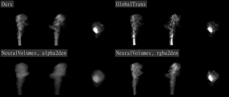
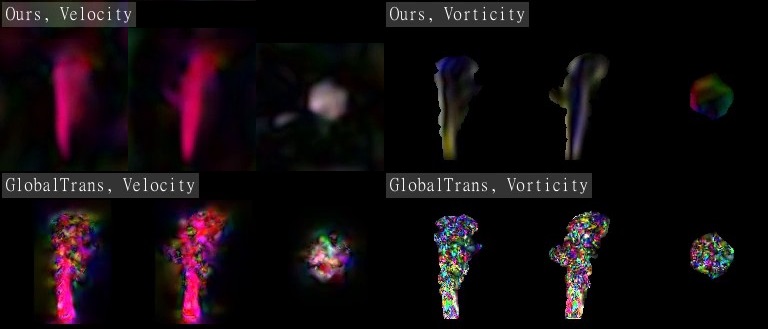
In the test on the synthetic data, a regular fluid flow is generated in resolution of . We simulate 120 steps with a time step of 0.5 (). The first 60 steps () are skipped as a startup and we use every second of the remaining 60 steps () as the target fluid fields to be reconstructed. For consistent comparison, the differentiable rendering of Global Transport [Franz et al., 2021] is used to render images at given time steps with a empirically determined lighting condition that roughly matches the lighting of the real captures, and black color is used as the background.
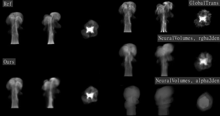
In the following, we first evaluate the proposed method (Ours) against related work including the Global Transport method [Franz et al., 2021] (GlobalTrans) and Neural Volumes [Lombardi et al., 2019] (NeuralVolumes). Then, to illustrate the role of each term in our supervision, ablation studies are presented with our full model and three ablated ones. We provide qualitative evaluations via rendered images and video clips (Sec. 1.1 of the supplemental webpage). Quantitative comparisons are given with the numerical errors on the reconstructed volumetric attributes (Table 1, 2).
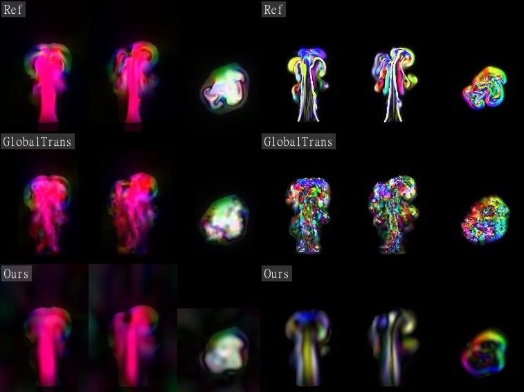
In the second and third columns of Table 1, we calculate the averaged errors, and , on the reconstructed density and velocity volume with regard to the reference. Note that the reference and results from previous work have a discretized representation, thus our results are sampled from our continuous models at uniform grid positions to compare consistently using numerical metrics. While our models and NeuralVolumes simply apply a 3D bounding box as the domain of the grid in , GlobalTrans performs optimization inside a time-varying visual hull which is projected from the 2D smoke region in the given images. All metrics are measured inside this visual hull with the inflow region (the bottom grid cells) excluded. Corresponding to the visualizations shown in Fig. 7, the density reconstructed by Ours and GlobalTrans achieves similar accuracy, but GlobalTrans exhibits high-frequency noise not present in the reference. However, the density reconstructed from the opacity of NeuralVolumes (denoted as ”alpha2den”) is rather uniform, leading to an error of . In addition, we generate another density via denoted as ”rgba2den”, which removes the “ghost density” and achieves an error of . This indicates that NeuralVolumes fails in the density-color disentanglement. While GlobalTrans has density and color disentangled based on the given lighting condition, our method manages to disentangle properly with the proposed growing strategy and the regularization term without knowing the lighting condition.
Velocity and vorticity visualizations use the middle slices from front, side, and top views. For all methods, we reduced the velocity intensity outside the visual hull for visualization, since the region with non-zero density is more important. NeuralVolumes does not provide a velocity field. Its results also exhibit discontinuity in time. GlobalTrans achieves better accuracy on the velocity but introduces high-frequency noise, which is also more visible in its vorticity field. The velocity of our method has the minimal error, smallest divergence, and small warping errors, as shown in the last three columns of the table.
Warp-Error MidWarp-Error
We compare the warping error using two metrics in Fig. 8. The first metric , denoted as ”Warp-Error”, represents a frame to frame warping. Denoted as ”MidWarp-Error”, the second metric shows the error between two consecutive density frames advected to the midpoint time using forward and backward warping, respectively. Note that all reconstruction models see images at time and , but the frames at the midpoint of are not given. The reference is numerically simulated with a time step of 0.5. GlobalTrans has the minimal frame-to-frame warping error which is even smaller than the reference, since it is trained to minimize the transport error at this discrete level. As a continuous method, Ours has a smaller midpoint warping error than the full step warping error, which is in consistent with the reference, and Ours has the smallest ”MidWarp-Error”. While it is rigorous to evaluate the warping metric at an unseen midpoint time, it is the situation in reality where continuous fluid phenomena are captured by cameras with limited frame-rates.
| Ours | 3.6264 | 0.4475 | 0.0353 | 0.2371 | 0.1581 |
|---|---|---|---|---|---|
| 3.4926 | 0.8786 | 0.0653 | 0.2359 | 0.2192 | |
| 3.8613 | 0.4883 | 0.0427 | 0.0905 | 0.0786 | |
| 3.5060 | 0.9127 | 0.0689 | 0.0466 | 0.0402 |
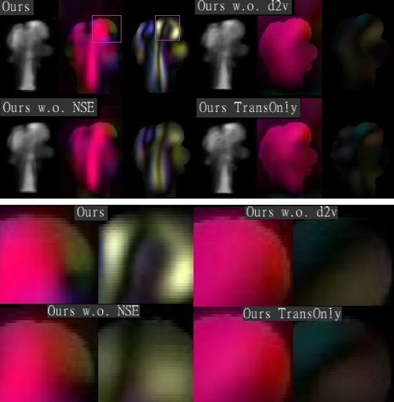
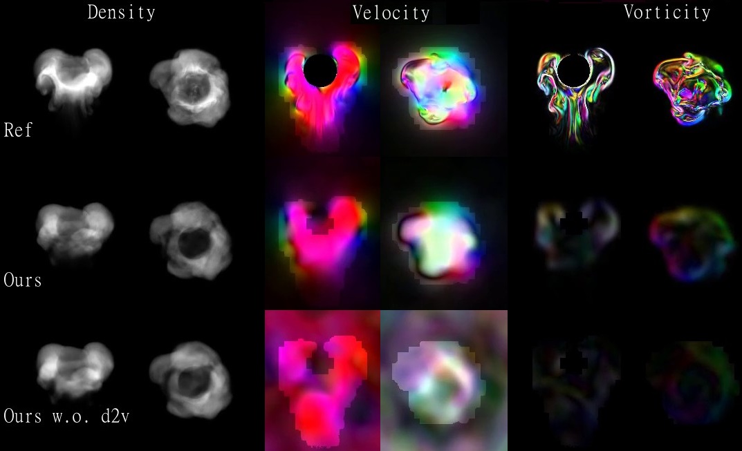
We further conduct ablation studies on the synthetic scene using the same evaluation metrics. In the first ablated model (Ours w.o. d2v), we remove , the term for vorticity compensation. The second ablated model (Ours w.o. NSE) has dropped the term to show the role of physical priors. In the last ablated model (Ours TransOnly), we remove both and , so that its velocity field is only supervised with the transport equation . The supervision applied on the radiance fields is not changed.
As shown in the first column of Table 2, our full and ablated models behave similarly on the density reconstruction, with an average error of 3.6212 and their differences in the range of . While Ours TransOnly has the smallest warping errors due to its velocity field only supervised by the transport equation, its velocity actually differs the most from the ground truth with an error of 0.9127. With our comprehensive supervision, Ours manages to reconstruct velocity more accurately. By comparing Ours w.o. d2v to Ours and comparing Ours TransOnly to Ours w.o. NSE, we see consistently that the former models without can only roughly match the reference velocity and have vorticity fields that are significantly underestimated. Merely using differentiable equations as objective functions, their nonlinearity makes the optimization process of the former models difficult. With the help of as model-based supervision, the latter models present enhanced vorticity and are much closer to the reference. Meanwhile, when comparing Ours w.o. NSE to Ours and comparing Ours TransOnly to Ours w.o. d2v, Navier-Stokes equations serve as physical priors and help in generating physically plausible but not necessarily correct solutions. We see that the latter models always have smaller divergence compared to the former ones. However, the result of Ours w.o. d2v shows little improvement over Ours TransOnly in Fig. 9, both suffering from vorticity underestimation. When using our full supervision, Navier-Stokes equations contribute more to the correct solution. Compared to Ours w.o. NSE, Ours presents sharper vorticity and has more details in the velocity fields.
Warp-Error MidWarp-Error
\begin{overpic}[width=433.62pt]{fig/Scalar/rwarp.png}
\put(82.0,1.0){\color[rgb]{1,1,1}\definecolor[named]{pgfstrokecolor}{rgb}{1,1,1}\pgfsys@color@gray@stroke{1}\pgfsys@color@gray@fill{1} GlobalTrans}
\put(90.0,36.0){\color[rgb]{1,1,1}\definecolor[named]{pgfstrokecolor}{rgb}{1,1,1}\pgfsys@color@gray@stroke{1}\pgfsys@color@gray@fill{1} Ours}
\put(32.0,1.0){\color[rgb]{1,1,1}\definecolor[named]{pgfstrokecolor}{rgb}{1,1,1}\pgfsys@color@gray@stroke{1}\pgfsys@color@gray@fill{1} GlobalTrans}
\put(40.0,36.0){\color[rgb]{1,1,1}\definecolor[named]{pgfstrokecolor}{rgb}{1,1,1}\pgfsys@color@gray@stroke{1}\pgfsys@color@gray@fill{1} Ours}
\end{overpic}
Real Captures
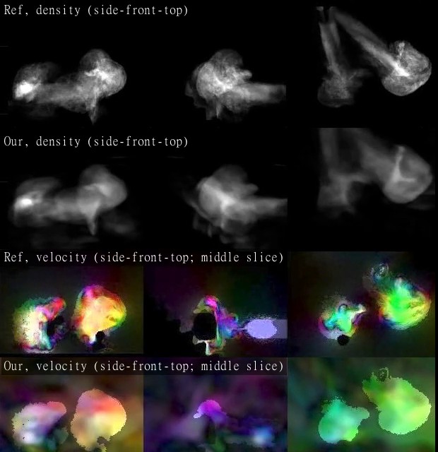
The real fluid captures of ScalarFlow have a frame-rate of 60. We take the middle 120 frames from each camera view for fluid reconstruction. With similar settings on camera calibration and lighting conditions, the conclusions for the real captures are consistent with the synthetic case. NeuralVolumes trivially encodes density information into color fields, as shown in Fig. 10. With given lighting conditions and visual hull applied, GlobalTrans generates detailed density and velocity fields with high-frequency noise. While our density volume is not as detailed as GlobalTrans, the rendered result in Fig. 6 corresponds well to the reference from a nearly opposite view. Ours also has smaller warping errors, which are visualized at the bottom of Fig. 10. Corresponding videos are presented in Sec. 1.2 of the supplemental webpage.
4.2. Synthetic Scenes with Complex Lighting
In this section, we show results of synthetic fluid scenes rendered using Blender with a complex lighting combination of point lights, directional lights and an environment map. The density volume is rendered with strong and non-linear attenuation as dense smoke. Since it is hard to approximate the lighting condition with point and ambient lights in this setting, the Global Transport method can hardly be applied to these scenes and is thus excluded in the comparison. In these scenes, we have five cameras evenly distributed on a circle with the target fluid in the center. All results are displayed with a dark green background, which is different to the background color used during training, and thus can be considered as being “transparent” with no density accumulated along the rays.
A Simple Plume Scene
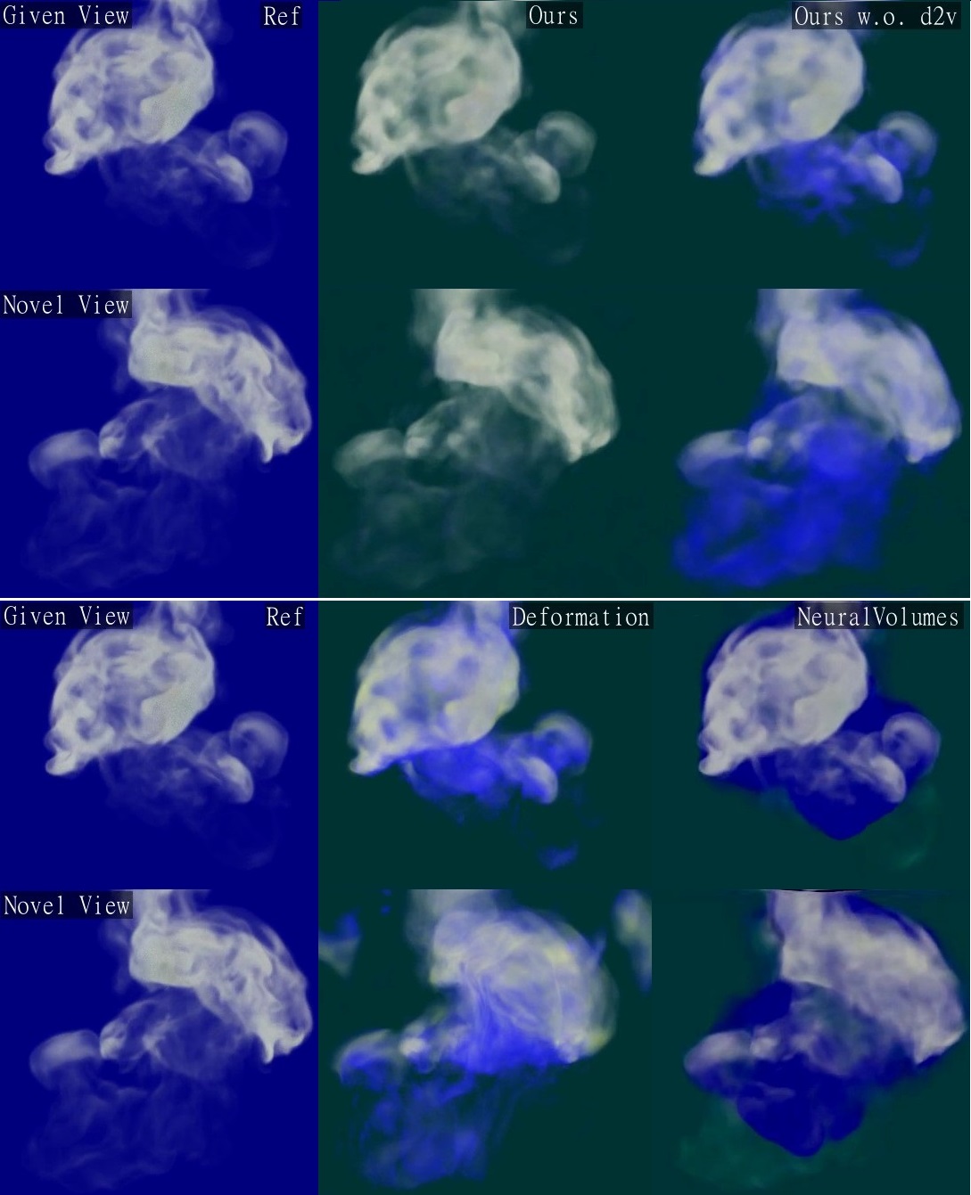
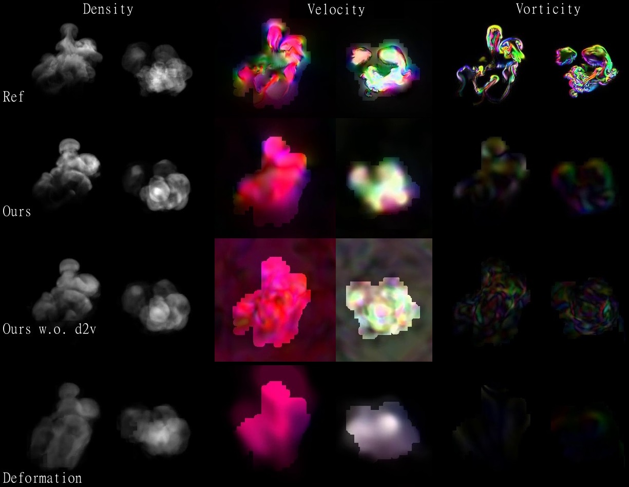
We first test with a regular plume scene in resolution of . 120 frames are used with a time step of 1.0. While the ScalarFlow dataset has a black background, the blue color is used in this case, as shown by the given view in Fig. 11. Due to the complex rendering setting with sparse views given, NeuralVolumes shows strong “ghost density” in blue. This artifact is largely reduced in Ours w.o. d2v with the help of , but is still visible at the bottom part with thin smoke. Our full model presents a good density estimation with “ghost density” hardly noticeable. This improvement over Ours w.o. d2v is mainly due to a more accurate velocity field. Considering the thin smoke at the bottom part of Ours w.o. d2v, a less accurate velocity field could warp them to a region expecting fluid density in white at some time, and warp them to a region expecting nothing or at least something in blue at some other time. The temporal inconsistency results in a “color bleeding” artifact that is slightly visible in given views and more visible in novel views.
Some related works [Tretschk et al., 2021; Li et al., 2020] explore dynamic NeRF, but most of them focus on scenes with deformable surfaces and introduce constraints that are not appropriate for fluids. While we do not compare to these methods due to the largely different reconstruction target, we train a Deformation model to illustrate the impact of inappropriate constraints. Learning a canonical spatial radiance field and a spatiotemporal deformation field , Deformation uses the same network architecture as ours. Their pixels are rendered with . As shown in Fig. 11, the Deformation model achieves quality similar to Ours w.o. d2v on the given view, but its density volume has unnatural stretches that are visible in novel views. From the visualization of the density at the bottom left, we can see the existence of “ghost density” at the bottom for the Deformation model and Ours w.o. d2v. While Deformation does not produce velocity fields directly, we calculated one from for visualization. As shown on the bottom of Fig. 11, the velocity calculated from is heavily constrained by the deformation and uniformly goes upward with almost zero vorticity. This relatively rigid deformation results in the stretches discussed above. Our full model generates density and velocity volumes that can roughly match the reference. The density in our result is more concentrated on the ”surface” since the reference fluid has nonlinear attenuation, which is not given but can easily be extended if provided. Videos of the plume scene are presented in Sec. 2.1 of the supplemental webpage.
Plume with a Regular Obstacle
While previous scenes have fluids as the sole target, we test hybrid scenes with obstacles in the following. The first hybrid scene has a regular obstacle in shape of a sphere. The simulation resolution is and 148 frames are simulated with a time step of 1.0. The background is set as white during training. As shown in the first row of Fig. 12, based on our hybrid architecture and the deferred temporal component, our full model has the static and dynamic components successfully separated. While our full model generates natural density volume without “ghost density”, the result of Ours w.o. d2v on the left of the second row is slightly blurry. NeuralVolumes contains “ghost density”. The baseline model of NeRF+T, which is the original ReLU-based NeRF model with time as an extended dimension, has problems dealing with the white background and results in “ghost density” fulfilling the domain. Due to the occlusion of the “ghost density”, there is a lack of supervision in the inner region and some density noise can be observed at novel views. Visualizations of velocity and vorticity are shown at the bottom, with ours closely resembling the reference. Its vorticity is also much stronger than Ours w.o. d2v. The supplemental webpage presents the videos for this scene in Sec. 2.2.
4.3. Complex Scenes with Arbitrary Obstacles
At last, we test our algorithm in complex scenes with obstacles of arbitrary shape under lighting composited by point lights, directional lights, as well as an environment map. The black color is used as the background during the training. Besides the five evenly distributed cameras on a circle, we use two more cameras viewing from above since the geometry is very challenging in the following scenes.
The Car Scene
The Car scene is simulated in resolution of for 148 steps with a time step of 1.0. While other scenes only have one or two small inflow regions, the whole domain of this scene uses a strong free stream velocity, whose direction is visualized as yellow on the right of Fig. 13. We simulate a shallow sheet of smoke passing through the car from the front top. The velocity field in this scene is particularly important for vehicle design, which can be used to calculate the drag force, the surface pressure, etc. Using our algorithm, the geometry of the car and the density of the smoke are nicely and separately reconstructed. While the reconstructed velocity roughly matches the reference, its vorticity is not as turbulent as the ground truth. This is mainly because smoke density is mixed together due to the strong vorticity in all directions at the wake of the car and the observed density derivatives in space and time are not as high as it should be. To improve on this particular case, it would be interesting to experiment with smoke in varying color or to apply frequency-based priors to constrain the vorticity.
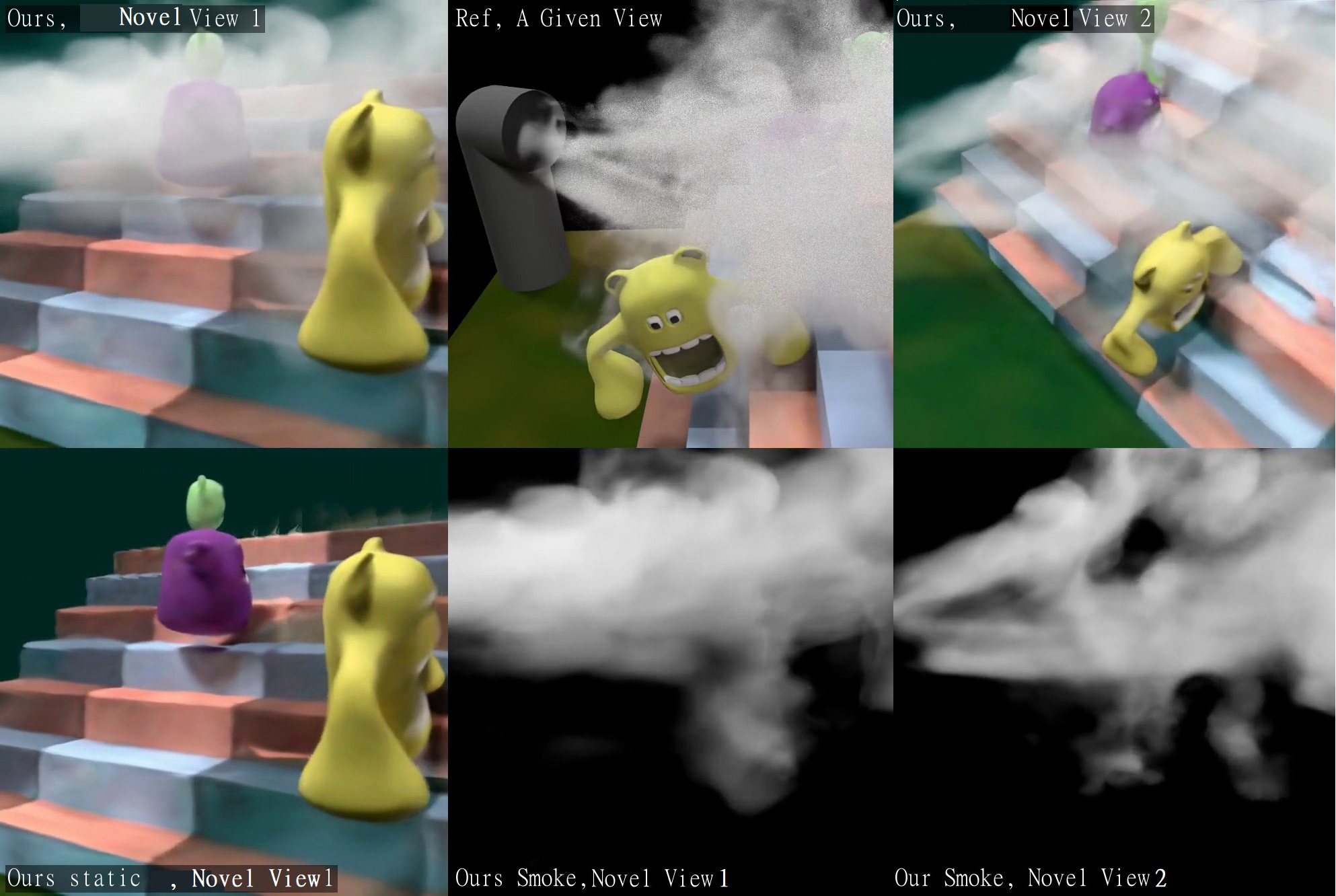
The Game Scene
In the Game scene, dense smoke is coming out of a tube and hitting three monsters on the stairs. It is in resolution of . 148 frames are simulated with a time step of 1.0. This scene represents a very difficult case due to the complex geometry, the occlusion caused by the close positioning of the monsters and stairs, the dense smoke hiding details inside, the strong motion at the interface of smoke and obstacles, and the moving shadow cast from the smoke. Faced with all these difficulties, our method manages to separate the static and dynamic components very well. While the inner region of the reconstructed smoke density is a little blurry, the rendered images have reasonable details on the outer bound area of the smoke. The complex geometry of obstacles are reconstructed reasonably well in general. The reconstructed velocity field can nicely resemble the complex ground truth, with smoke density accurately flowing around obstacles other than passing through.
4.4. Results Summary and Limitations
To summarize, we have tested our algorithm on real and synthetic fluid scenes. For synthetic simulations, we have used buoyant and stream flow, with and without inflow, with and without obstacles in regular and arbitrary shapes. For the rendering, we have used dense and thin smoke, linear and nonlinear attenuation, simple and complex lighting conditions.
We observe consistent results provided by our model: “Ghost density” is successfully removed in density fields as an appropriate disentanglement of density and color. The resulting velocity generally matches the reference and showing enhanced vorticity than purely PINN-based learning. Additionally, our hybrid model separately reconstructs static and dynamic components without using additional manual labeling. The limitations of our method mainly pertain to non-linear aspects of the optimization process and slow training caused by the PDEs calculation via auto-differentiation. While there is room for improvement on the high-frequency details of the reconstructed velocity field, end-to-end estimation of velocity from images is a difficult task, and the proposed model-based supervision yields significant improvements. Applying frequency-based supervision [Yifan et al., 2022] on the velocity would be an interesting future avenue. Also, the training of a single NeRF model is not efficient due to prohibitive queries of the neural networks. Training our algorithm with a hybrid architecture and a PINN-based velocity model on the dynamic data is around three times slower than that. Training details including hyper-parameters and training time for each scene is provided in the supplemental material, for e.g., the Game scene takes 64 hours when using a single NVIDIA Quadro RTX 8000 GPU. With the recent progress in fast neural representation training [Yu et al., 2021; Müller et al., 2022], we anticipate this limitation to be resolved in the near future. Besides code optimization and the use of multiple GPUs, breaking down large-scale scenes in space can make their reconstructions more efficient. Our fluid reconstruction can be used to enhance physical understanding from videos. The reconstructed fields can also be used in graphics applications. In contrast with forward simulation methods that allow fluid animations to be designed using initial conditions and physical parameters, reconstruction methods like ours allow users to generate fluid phenomena from video captures. In order to present fluid animations with fine-level detail, it would be interesting to apply our approach together with detail synthesis [Xie et al., 2018] or fluid guiding [Forootaninia and Narain, 2020].
5. Conclusions
We have introduced an optimization-based algorithm that is able to reconstruct continuous fluid fields end-to-end from a sparse set of video frames based on the developed spatio-temporal neural representation for dynamic fluid flow and the underlying physics-informed learning mechanisms. To the best of our knowledge, this is the first method to allow flow motion to be reconstructed from image captures of hybrid scenes with both fluid and arbitrary obstacles, while being agnostic to initial, boundary, or lighting conditions. In our optimization framework, we jointly apply supervision from images, physical priors, as well as data prior encoded as a pre-trained model. With the comprehensive supervisions, our method exhibits stable effectiveness and strong flexibility on a wide range of scenes.
We see our method as an crucial step towards capturing and analyzing real fluid phenomena with relaxed constraints, e.g. allowing captures under changing illumination. With the advantage of handling scenes with unknown obstacles and lighting, we are especially interested in exploring in-the-wild fluid capture as well as more elaborate fluid-obstacle interactions in the future.
Acknowledgements.
The project was supported by the ERC Consolidator Grant 4DRepLy (770784). Mengyu Chu and Lingjie Liu were supported by Lise Meitner Postdoctoral Fellowships.References
- [1]
- Atcheson et al. [2009] Bradley Atcheson, Wolfgang Heidrich, and Ivo Ihrke. 2009. An evaluation of optical flow algorithms for background oriented schlieren imaging. Experiments in Fluids 46, 3 (01 Mar 2009), 467–476. https://doi.org/10.1007/s00348-008-0572-7
- Bauer et al. [2015] Peter Bauer, Alan Thorpe, and Gilbert Brunet. 2015. The quiet revolution of numerical weather prediction. Nature 525, 7567 (2015), 47–55.
- Berg and Nyström [2018] Jens Berg and Kaj Nyström. 2018. A unified deep artificial neural network approach to partial differential equations in complex geometries. Neurocomputing 317 (2018), 28–41. https://doi.org/10.1016/j.neucom.2018.06.056
- Bridson [2015] Robert Bridson. 2015. Fluid simulation for computer graphics. CRC press.
- Broxton et al. [2020] Michael Broxton, John Flynn, Ryan Overbeck, Daniel Erickson, Peter Hedman, Matthew Duvall, Jason Dourgarian, Jay Busch, Matt Whalen, and Paul Debevec. 2020. Immersive light field video with a layered mesh representation. ACM Transactions on Graphics (TOG) 39, 4 (2020), 86–1.
- Bushnell and Moore [1991] Dennis M Bushnell and KJ Moore. 1991. Drag reduction in nature. Annual review of fluid mechanics 23, 1 (1991), 65–79.
- Chabra et al. [2020] Rohan Chabra, Jan E Lenssen, Eddy Ilg, Tanner Schmidt, Julian Straub, Steven Lovegrove, and Richard Newcombe. 2020. Deep local shapes: Learning local SDF priors for detailed 3D reconstruction. In European Conference on Computer Vision. Springer, 608–625.
- Chen et al. [2021] Jianchuan Chen, Ying Zhang, Di Kang, Xuefei Zhe, Linchao Bao, and Huchuan Lu. 2021. Animatable Neural Radiance Fields from Monocular RGB Video. arXiv:2106.13629 [cs.CV]
- Chen and Zhang [2019] Zhiqin Chen and Hao Zhang. 2019. Learning implicit fields for generative shape modeling. In Proceedings of the IEEE/CVF Conference on Computer Vision and Pattern Recognition. 5939–5948.
- Chibane et al. [2020] Julian Chibane, Gerard Pons-Moll, et al. 2020. Neural Unsigned Distance Fields for Implicit Function Learning. Advances in Neural Information Processing Systems 33 (2020).
- Chu et al. [2021] Mengyu Chu, Nils Thuerey, Hans-Peter Seidel, Christian Theobalt, and Rhaleb Zayer. 2021. Learning meaningful controls for fluids. ACM Transactions on Graphics (TOG) 40, 4 (2021), 1–13.
- Chu et al. [2020] Mengyu Chu, You Xie, Jonas Mayer, Laura Leal-Taixé, and Nils Thuerey. 2020. Learning temporal coherence via self-supervision for GAN-based video generation. ACM Transactions on Graphics (TOG) 39, 4 (2020), 75–1.
- Eckert et al. [2019] Marie-Lena Eckert, Kiwon Um, and Nils Thuerey. 2019. ScalarFlow: a large-scale volumetric data set of real-world scalar transport flows for computer animation and machine learning. ACM Transactions on Graphics (TOG) 38, 6 (2019), 1–16.
- Elsinga et al. [2006] Gerrit E Elsinga, Fulvio Scarano, Bernhard Wieneke, and Bas W van Oudheusden. 2006. Tomographic particle image velocimetry. Experiments in fluids 41, 6 (2006), 933–947.
- Eslami et al. [2018] SM Ali Eslami, Danilo Jimenez Rezende, Frederic Besse, Fabio Viola, Ari S Morcos, Marta Garnelo, Avraham Ruderman, Andrei A Rusu, Ivo Danihelka, Karol Gregor, et al. 2018. Neural scene representation and rendering. Science 360, 6394 (2018), 1204–1210.
- Forootaninia and Narain [2020] Zahra Forootaninia and Rahul Narain. 2020. Frequency-domain smoke guiding. ACM Transactions on Graphics (TOG) 39, 6 (2020), 1–10.
- Franz et al. [2021] Erik Franz, Barbara Solenthaler, and Nils Thuerey. 2021. Global Transport for Fluid Reconstruction with Learned Self-Supervision. In Proceedings of the IEEE/CVF Conference on Computer Vision and Pattern Recognition. 1632–1642.
- Gafni et al. [2020] Guy Gafni, Justus Thies, Michael Zollhoefer, and Matthias Niessner. 2020. Dynamic Neural Radiance Fields for Monocular 4D Facial Avatar Reconstruction. arXiv:2012.03065 [cs.CV]
- Garbin et al. [2021] Stephan J Garbin, Marek Kowalski, Matthew Johnson, Jamie Shotton, and Julien Valentin. 2021. Fastnerf: High-fidelity neural rendering at 200fps. arXiv preprint arXiv:2103.10380 (2021).
- Geng et al. [2020] Zhenglin Geng, Daniel Johnson, and Ronald Fedkiw. 2020. Coercing machine learning to output physically accurate results. J. Comput. Phys. 406 (2020), 109099.
- Gibou et al. [2019] Frederic Gibou, David Hyde, and Ron Fedkiw. 2019. Sharp interface approaches and deep learning techniques for multiphase flows. J. Comput. Phys. 380 (2019), 442–463.
- Granskog et al. [2020] Jonathan Granskog, Fabrice Rousselle, Marios Papas, and Jan Novák. 2020. Compositional neural scene representations for shading inference. ACM Transactions on Graphics (TOG) 39, 4 (2020), 135–1.
- Grant [1997] I. Grant. 1997. Particle Image Velocimetry: a Review. Proceedings of the Institution of Mechanical Engineers 211, 1 (1997), 55–76.
- Gregson et al. [2014] James Gregson, Ivo Ihrke, Nils Thuerey, and Wolfgang Heidrich. 2014. From capture to simulation: connecting forward and inverse problems in fluids. ACM Transactions on Graphics (TOG) 33, 4 (2014), 1–11.
- Gu et al. [2021] Jiatao Gu, Lingjie Liu, Peng Wang, and Christian Theobalt. 2021. StyleNeRF: A Style-based 3D-Aware Generator for High-resolution Image Synthesis. arXiv:2110.08985 [cs.CV]
- Gu et al. [2013] Jinwei Gu, S.K. Nayar, E. Grinspun, P.N. Belhumeur, and R. Ramamoorthi. 2013. Compressive Structured Light for Recovering Inhomogeneous Participating Media. PAMI 35, 3 (2013), 555–567.
- He et al. [2000] S. He, K. Reif, and R. Unbehauen. 2000. Multilayer Neural Networks for Solving a Class of Partial Differential Equations. Neural Netw. 13, 3 (apr 2000), 385–396. https://doi.org/10.1016/S0893-6080(00)00013-7
- Hedman et al. [2021] Peter Hedman, Pratul P. Srinivasan, Ben Mildenhall, Jonathan T. Barron, and Paul Debevec. 2021. Baking Neural Radiance Fields for Real-Time View Synthesis. ICCV (2021).
- Ji et al. [2013] Yu Ji, Jinwei Ye, and Jingyi Yu. 2013. Reconstructing Gas Flows Using Light-Path Approximation. In Proceedings of the IEEE Conference on Computer Vision and Pattern Recognition (CVPR).
- Kim et al. [2008] Theodore Kim, Nils Thuerey, Doug James, and Markus Gross. 2008. Wavelet turbulence for fluid simulation. ACM Transactions on Graphics (TOG) 27, 3 (2008), 1–6.
- Kwon et al. [2021] Youngjoong Kwon, Dahun Kim, Duygu Ceylan, and Henry Fuchs. 2021. Neural Human Performer: Learning Generalizable Radiance Fields for Human Performance Rendering. NeurIPS (2021).
- Lagaris et al. [1998] I.E. Lagaris, A. Likas, and D.I. Fotiadis. 1998. Artificial neural networks for solving ordinary and partial differential equations. IEEE Transactions on Neural Networks 9, 5 (1998), 987–1000. https://doi.org/10.1109/72.712178
- Ledig et al. [2017] Christian Ledig, Lucas Theis, Ferenc Huszár, Jose Caballero, Andrew Cunningham, Alejandro Acosta, Andrew Aitken, Alykhan Tejani, Johannes Totz, Zehan Wang, et al. 2017. Photo-realistic single image super-resolution using a generative adversarial network. In Proceedings of the IEEE conference on computer vision and pattern recognition. 4681–4690.
- Li et al. [2020] Z. Li, Simon Niklaus, Noah Snavely, and Oliver Wang. 2020. Neural Scene Flow Fields for Space-Time View Synthesis of Dynamic Scenes. ArXiv abs/2011.13084 (2020).
- Liu et al. [2020] Lingjie Liu, Jiatao Gu, Kyaw Zaw Lin, Tat-Seng Chua, and Christian Theobalt. 2020. Neural Sparse Voxel Fields. Advances in Neural Information Processing Systems 33 (2020).
- Liu et al. [2021] Lingjie Liu, Marc Habermann, Viktor Rudnev, Kripasindhu Sarkar, Jiatao Gu, and Christian Theobalt. 2021. Neural Actor: Neural Free-view Synthesis of Human Actors with Pose Control. ACM Trans. Graph.(ACM SIGGRAPH Asia) (2021).
- Lombardi et al. [2019] Stephen Lombardi, Tomas Simon, Jason Saragih, Gabriel Schwartz, Andreas Lehrmann, and Yaser Sheikh. 2019. Neural volumes: learning dynamic renderable volumes from images. ACM Transactions on Graphics (TOG) 38, 4 (2019), 1–14.
- Lombardi et al. [2021] Stephen Lombardi, Tomas Simon, Gabriel Schwartz, Michael Zollhoefer, Yaser Sheikh, and Jason Saragih. 2021. Mixture of Volumetric Primitives for Efficient Neural Rendering. arXiv:2103.01954 [cs.GR]
- Mai-Duy and Tran-Cong [2003] Nam Mai-Duy and Thanh Tran-Cong. 2003. Approximation of function and its derivatives using radial basis function networks. Applied Mathematical Modelling 27, 3 (2003), 197–220. https://doi.org/10.1016/S0307-904X(02)00101-4
- Mildenhall et al. [2019] Ben Mildenhall, Pratul P Srinivasan, Rodrigo Ortiz-Cayon, Nima Khademi Kalantari, Ravi Ramamoorthi, Ren Ng, and Abhishek Kar. 2019. Local light field fusion: Practical view synthesis with prescriptive sampling guidelines. ACM Transactions on Graphics (TOG) 38, 4 (2019), 1–14.
- Mildenhall et al. [2020] Ben Mildenhall, Pratul P. Srinivasan, Matthew Tancik, Jonathan T. Barron, Ravi Ramamoorthi, and Ren Ng. 2020. NeRF: Representing Scenes as Neural Radiance Fields for View Synthesis. In ECCV.
- Müller et al. [2022] Thomas Müller, Alex Evans, Christoph Schied, and Alexander Keller. 2022. Instant Neural Graphics Primitives with a Multiresolution Hash Encoding. arXiv preprint arXiv:2201.05989 (2022).
- Niemeyer and Geiger [2021] Michael Niemeyer and Andreas Geiger. 2021. GIRAFFE: Representing Scenes as Compositional Generative Neural Feature Fields. In Proc. IEEE Conf. on Computer Vision and Pattern Recognition (CVPR).
- Niemeyer et al. [2020] Michael Niemeyer, Lars Mescheder, Michael Oechsle, and Andreas Geiger. 2020. Differentiable volumetric rendering: Learning implicit 3d representations without 3d supervision. In Proceedings of the IEEE/CVF Conference on Computer Vision and Pattern Recognition. 3504–3515.
- Oechsle et al. [2021] Michael Oechsle, Songyou Peng, and Andreas Geiger. 2021. UNISURF: Unifying Neural Implicit Surfaces and Radiance Fields for Multi-View Reconstruction. In International Conference on Computer Vision (ICCV).
- Pakravan et al. [2021] Samira Pakravan, Pouria A. Mistani, Miguel A. Aragon-Calvo, and Frederic Gibou. 2021. Solving inverse-PDE problems with physics-aware neural networks. J. Comput. Phys. 440 (2021), 110414.
- Park et al. [2019] Jeong Joon Park, Peter Florence, Julian Straub, Richard Newcombe, and Steven Lovegrove. 2019. DeepSDF: Learning continuous signed distance functions for shape representation. In Proceedings of the IEEE/CVF Conference on Computer Vision and Pattern Recognition. 165–174.
- Park et al. [2020] Keunhong Park, Utkarsh Sinha, Jonathan T. Barron, Sofien Bouaziz, Dan B Goldman, Steven M. Seitz, and Ricardo Martin-Brualla. 2020. Deformable Neural Radiance Fields. arXiv preprint arXiv:2011.12948 (2020).
- Park et al. [2021] Keunhong Park, Utkarsh Sinha, Peter Hedman, Jonathan T. Barron, Sofien Bouaziz, Dan B Goldman, Ricardo Martin-Brualla, and Steven M. Seitz. 2021. HyperNeRF: A Higher-Dimensional Representation for Topologically Varying Neural Radiance Fields. ACM Trans. Graph. 40, 6, Article 238 (dec 2021).
- Peng et al. [2021a] Sida Peng, Junting Dong, Qianqian Wang, Shangzhan Zhang, Qing Shuai, Hujun Bao, and Xiaowei Zhou. 2021a. Animatable Neural Radiance Fields for Human Body Modeling. ICCV (2021).
- Peng et al. [2020] Songyou Peng, Michael Niemeyer, Lars Mescheder, Marc Pollefeys, and Andreas Geiger. 2020. Convolutional occupancy networks. In Computer Vision–ECCV 2020: 16th European Conference, Glasgow, UK, August 23–28, 2020, Proceedings, Part III 16. Springer, 523–540.
- Peng et al. [2021b] Sida Peng, Yuanqing Zhang, Yinghao Xu, Qianqian Wang, Qing Shuai, Hujun Bao, and Xiaowei Zhou. 2021b. Neural Body: Implicit Neural Representations with Structured Latent Codes for Novel View Synthesis of Dynamic Humans. In CVPR.
- Philip et al. [2019] Julien Philip, Michaël Gharbi, Tinghui Zhou, Alexei A Efros, and George Drettakis. 2019. Multi-view relighting using a geometry-aware network. ACM Transactions on Graphics (TOG) 38, 4 (2019), 1–14.
- Qiu et al. [2021] Sheng Qiu, Chen Li, Changbo Wang, and Hong Qin. 2021. A Rapid, End-to-end, Generative Model for Gaseous Phenomena from Limited Views. (2021). https://doi.org/10.1111/cgf.14270
- Raissi et al. [2019] M. Raissi, P. Perdikaris, and G.E. Karniadakis. 2019. Physics-informed neural networks: A deep learning framework for solving forward and inverse problems involving nonlinear partial differential equations. J. Comput. Phys. 378 (2019), 686–707. https://doi.org/10.1016/j.jcp.2018.10.045
- Raissi et al. [2020] Maziar Raissi, Alireza Yazdani, and George Em Karniadakis. 2020. Hidden fluid mechanics: Learning velocity and pressure fields from flow visualizations. Science 367, 6481 (2020), 1026–1030.
- Raj et al. [2021] Amit Raj, Michael Zollhoefer, Tomas Simon, Jason Saragih, Shunsuke Saito, James Hays, and Stephen Lombardi. 2021. PVA: Pixel-aligned Volumetric Avatars. arXiv:2101.02697 [cs.CV]
- Reiser et al. [2021] Christian Reiser, Songyou Peng, Yiyi Liao, and Andreas Geiger. 2021. KiloNeRF: Speeding up Neural Radiance Fields with Thousands of Tiny MLPs. In International Conference on Computer Vision (ICCV).
- Saito et al. [2019] Shunsuke Saito, Zeng Huang, Ryota Natsume, Shigeo Morishima, Angjoo Kanazawa, and Hao Li. 2019. PIFu: Pixel-aligned implicit function for high-resolution clothed human digitization. In Proceedings of the IEEE/CVF International Conference on Computer Vision. 2304–2314.
- Schwarz et al. [2020] Katja Schwarz, Yiyi Liao, Michael Niemeyer, and Andreas Geiger. 2020. GRAF: Generative Radiance Fields for 3D-Aware Image Synthesis. Advances in Neural Information Processing Systems 33 (2020).
- Shi et al. [2010] Kuangyu Shi, Michael Souvatzoglou, Sabrina T Astner, Peter Vaupel, Fridtjof Nüsslin, Jan J Wilkens, and Sibylle I Ziegler. 2010. Quantitative assessment of hypoxia kinetic models by a cross-study of dynamic 18F-FAZA and 15O-H2O in patients with head and neck tumors. Journal of Nuclear Medicine 51, 9 (2010), 1386–1394.
- Sirignano and Spiliopoulos [2018] Justin Sirignano and Konstantinos Spiliopoulos. 2018. DGM: A deep learning algorithm for solving partial differential equations. J. Comput. Phys. 375 (Dec 2018), 1339–1364. https://doi.org/10.1016/j.jcp.2018.08.029
- Sitzmann et al. [2020] Vincent Sitzmann, Julien N.P. Martel, Alexander W. Bergman, David B. Lindell, and Gordon Wetzstein. 2020. Implicit Neural Representations with Periodic Activation Functions. In Proc. NeurIPS.
- Sitzmann et al. [2019a] Vincent Sitzmann, Justus Thies, Felix Heide, Matthias Nießner, Gordon Wetzstein, and Michael Zollhofer. 2019a. DeepVoxels: Learning persistent 3D feature embeddings. In Proceedings of the IEEE/CVF Conference on Computer Vision and Pattern Recognition. 2437–2446.
- Sitzmann et al. [2019b] Vincent Sitzmann, Michael Zollhöfer, and Gordon Wetzstein. 2019b. Scene representation networks: Continuous 3D-structure-aware neural scene representations. In Advances in Neural Information Processing Systems. 1121–1132.
- Srinivasan et al. [2021] Pratul P Srinivasan, Boyang Deng, Xiuming Zhang, Matthew Tancik, Ben Mildenhall, and Jonathan T Barron. 2021. NeRV: Neural reflectance and visibility fields for relighting and view synthesis. In Proceedings of the IEEE/CVF Conference on Computer Vision and Pattern Recognition. 7495–7504.
- Srinivasan et al. [2019] Pratul P Srinivasan, Richard Tucker, Jonathan T Barron, Ravi Ramamoorthi, Ren Ng, and Noah Snavely. 2019. Pushing the boundaries of view extrapolation with multiplane images. In Proceedings of the IEEE/CVF Conference on Computer Vision and Pattern Recognition. 175–184.
- Su et al. [2021] Shih-Yang Su, Frank Yu, Michael Zollhoefer, and Helge Rhodin. 2021. A-NeRF: Surface-free Human 3D Pose Refinement via Neural Rendering. arXiv preprint arXiv:2102.06199 (2021).
- Tancik et al. [2020] Matthew Tancik, Pratul P. Srinivasan, Ben Mildenhall, Sara Fridovich-Keil, Nithin Raghavan, Utkarsh Singhal, Ravi Ramamoorthi, Jonathan T. Barron, and Ren Ng. 2020. Fourier Features Let Networks Learn High Frequency Functions in Low Dimensional Domains. NeurIPS (2020).
- Thuerey and Pfaff [2018] Nils Thuerey and Tobias Pfaff. 2018. MantaFlow. http://mantaflow.com.
- Tretschk et al. [2021] Edgar Tretschk, Ayush Tewari, Vladislav Golyanik, Michael Zollhöfer, Christoph Lassner, and Christian Theobalt. 2021. Non-Rigid Neural Radiance Fields: Reconstruction and Novel View Synthesis of a Dynamic Scene From Monocular Video. In IEEE International Conference on Computer Vision (ICCV). IEEE.
- Um et al. [2020] Kiwon Um, Robert Brand, Yun Raymond Fei, Philipp Holl, and Nils Thuerey. 2020. Solver-in-the-loop: Learning from differentiable physics to interact with iterative pde-solvers. Advances in Neural Information Processing Systems 33 (2020), 6111–6122.
- Wang et al. [2021] Peng Wang, Lingjie Liu, Yuan Liu, Christian Theobalt, Taku Komura, and Wenping Wang. 2021. NeuS: Learning Neural Implicit Surfaces by Volume Rendering for Multi-view Reconstruction. NeurIPS (2021).
- Wang et al. [2020] Ziyan Wang, Timur Bagautdinov, Stephen Lombardi, Tomas Simon, Jason Saragih, Jessica Hodgins, and Michael Zollhöfer. 2020. Learning Compositional Radiance Fields of Dynamic Human Heads. arXiv:2012.09955 [cs.CV]
- Xian et al. [2020] Wenqi Xian, Jia-Bin Huang, Johannes Kopf, and Changil Kim. 2020. Space-time Neural Irradiance Fields for Free-Viewpoint Video. arXiv:2011.12950 [cs.CV]
- Xie et al. [2018] You Xie, Erik Franz, Mengyu Chu, and Nils Thuerey. 2018. tempoGAN: A Temporally Coherent, Volumetric GAN for Super-resolution Fluid Flow. ACM Transactions on Graphics (TOG) 37, 4 (2018), 95.
- Xiong et al. [2017] Jinhui Xiong, Ramzi Idoughi, Andres A Aguirre-Pablo, Abdulrahman B Aljedaani, Xiong Dun, Qiang Fu, Sigurdur T Thoroddsen, and Wolfgang Heidrich. 2017. Rainbow particle imaging velocimetry for dense 3D fluid velocity imaging. ACM Transactions on Graphics (TOG) 36, 4 (2017), 1–14.
- Yariv et al. [2021] Lior Yariv, Jiatao Gu, Yoni Kasten, and Yaron Lipman. 2021. Volume rendering of neural implicit surfaces. In Thirty-Fifth Conference on Neural Information Processing Systems.
- Yariv et al. [2020] Lior Yariv, Yoni Kasten, Dror Moran, Meirav Galun, Matan Atzmon, Basri Ronen, and Yaron Lipman. 2020. Multiview Neural Surface Reconstruction by Disentangling Geometry and Appearance. Advances in Neural Information Processing Systems 33 (2020).
- Yifan et al. [2022] Wang Yifan, Lukas Rahmann, and Olga Sorkine-hornung. 2022. Geometry-Consistent Neural Shape Representation with Implicit Displacement Fields. In International Conference on Learning Representations.
- Yifan et al. [2019] Wang Yifan, Felice Serena, Shihao Wu, Cengiz Öztireli, and Olga Sorkine-Hornung. 2019. Differentiable surface splatting for point-based geometry processing. ACM Transactions on Graphics (TOG) 38, 6 (2019), 1–14.
- Yu et al. [2021] Alex Yu, Ruilong Li, Matthew Tancik, Hao Li, Ren Ng, and Angjoo Kanazawa. 2021. PlenOctrees for Real-time Rendering of Neural Radiance Fields. In ICCV.
- Zang et al. [2020] Guangming Zang, Ramzi Idoughi, Congli Wang, Anthony Bennett, Jianguo Du, Scott Skeen, William L. Roberts, Peter Wonka, and Wolfgang Heidrich. 2020. TomoFluid: Reconstructing Dynamic Fluid from Sparse View Videos. In Proceedings of the IEEE Conference on Computer Vision and Pattern Recognition. IEEE. https://repository.kaust.edu.sa/handle/10754/662380
- Zhang et al. [2021] Xiuming Zhang, Sean Fanello, Yun-Ta Tsai, Tiancheng Sun, Tianfan Xue, Rohit Pandey, Sergio Orts-Escolano, Philip Davidson, Christoph Rhemann, Paul Debevec, et al. 2021. Neural light transport for relighting and view synthesis. ACM Transactions on Graphics (TOG) 40, 1 (2021), 1–17.
- Zheng et al. [2021] Quan Zheng, Gurprit Singh, and Hans-Peter Seidel. 2021. Neural Relightable Participating Media Rendering. Advances in Neural Information Processing Systems 34 (2021).
- Zhou et al. [2018] Tinghui Zhou, Richard Tucker, John Flynn, Graham Fyffe, and Noah Snavely. 2018. Stereo magnification: learning view synthesis using multiplane images. ACM Transactions on Graphics (TOG) 37, 4 (2018), 1–12.