Chiral SQUID-metamaterial waveguide for circuit-QED

Abstract

Superconducting metamaterials, which are designed and fabricated with structured fundamental circuit elements, have motivated recent developments of exploring unconventional quantum phenomena in circuit quantum electrodynamics (circuit-QED). We propose a method to engineer 1D Josephson metamaterial as a chiral waveguide by considering a programmed spatiotemporal modulation on its effective impedance. The modulation currents are in the form of travelling waves which phase velocities are much slower than the propagation speed of microwave photons. Due to the Brillouin-scattering process, non-trivial spectrum regimes where photons can propagate unidirectionally emerge. Considering superconducting qubits coupling with this metamaterial waveguide, we analyze both Markovian and non-Markovian quantum dynamics, and find that superconducting qubits can dissipate photons unidirectionally. Moreover, we show that our proposal can be extended a cascaded quantum network with multiple nodes, where chiral photon transport between remote qubits can be realized. Our work might open the possibilities to exploit SQUID metamaterials for realizing unidirectional photon transport in circuit-QED platforms.

I introduction

The interaction between matter and quantized electromagnetic fields has been the central topic of quantum optics for more than half a century Lamb and Retherford (1947); Scully and Zubairy (1997); Cohen-Tannoudji et al. (1998); Walls and Milburn (2007); Clerk et al. (2010). The impressive progresses in quantum electrodynamics (QED) and quantum technologies provide solid foundations for quantum information science Clerk et al. (2010); Buluta et al. (2011); Xiang et al. (2013); Underwood et al. (2012); Reiserer and Rempe (2015); Chang et al. (2018). In past two decades, superconducting quantum circuits (SQCs) with Josephson junctions have been developed as a well-performed artificial platform for microwave photonics  Nakamura et al. (1999); Blais et al. (2004); Koch et al. (2007); Clarke and Wilhelm (2008); You and Nori (2011); Gu et al. (2017); et al. (2019a); Clerk et al. (2020); Blais et al. (2021); et al. (2021). The versatility of SQCs stems from the flexibilities in both fabrication and controlling processes, which allows to realize many exotic quantum phenomena such as dynamical Casimir effects and ultrastrong light–matter couplings Johansson et al. (2009, 2010); et al. (2011); Lähteenmäki et al. (2013); et al. (2011); Beaudoin et al. (2011); Kockum et al. (2019); Bourassa et al. (2009); et al. (2010).

In circuit-QED the boson modes of microwave photons are routinely supported by conventional circuit elements such as LC resonators, transmission-line resonators and 1D open coplanar-waveguides et al. (2007, 2008); Bourassa et al. (2012); Clem (2013); Doerner et al. (2018). Recently exploring intriguing QED phenomena with metamaterial structures in SQCs have attracted a lot of interests Leib et al. (2012); Liu and Houck (2017); et al. (2017); Kollár et al. (2019); Ma et al. (2019); Carusotto et al. (2020); Mazhorin et al. (2022). Compared with standard circuit-QED elements, superconducting metamaterials can be designed and fabricated in various kinds of spatial structures, which might have exotic band spectrum and nontrivial vacuum modes Mirhosseini et al. (2018); Scigliuzzo et al. (2021). For example, by engineering the hopping rates among microwave resonators or SQC qubits, the photonic metamaterials analogue to topological lattices and strongly correlated matters were realized Roushan et al. (2017); Kim et al. (2021). When the inductors and capacitors in the usual discrete model of a 1D transmission line are interchanged, the left-handed metamaterials can also be fabricated, which might work as a waveguide with an effective negative index of refraction Caloz et al. (2004); Egger and Wilhelm (2013); et al. (2019b); Messinger et al. (2019); Indrajeet et al. (2020).

The Josephson-chain metamaterials, which inherit the advantages of Josephson junctions such as nonlinearity and tunability, have been widely employed for different quantum engineering tasks Masluk et al. (2012); Altimiras et al. (2013); Weissl (2014); et al. (2015); Krupko and Nguyen (2018); Cosmic et al. (2018); Planat et al. (2020); Esposito et al. (2022); Sinha et al. (2022). For example, many-body quantum optics in ultra-strong coupling regimes was successfully demonstrated in a Josephson chain platform by exploiting its high characteristic impedance et al. (2019c). Moreover, given that each node junction is replaced with a superconducting quantum interference device (SQUID), the SQUID chain is possible to be engineered as a tunable high-impedance ohmic reservoir by applying position-dependent magnetic flux Rastelli and Pop (2018). When the SQUID chain are biased with a space-time varying flux, analogue Hawking radiation can be reproduced  Nation et al. (2009, 2012); Tian et al. (2017); Tian and Du (2019); Lang and Schützhold (2019); Blencowe and Wang (2020). To create an event horizon, the group velocity of the modulation signals should be comparable to the propagation velocity.

In contrast to proposals which are analogs of creating cosmological particles Nation et al. (2009); Lang and Schützhold (2019), in this study we focus on the parameter regime where the velocity of the modulation signals is much slower than the photon’s propagation speed, which was rarely considered in previous studies. The scenario is akin to realizing nonreciprocal sound propagation in an elastic metamaterial via spatiotemporally modulating the stiffness Swinteck et al. (2015); Trainiti and Ruzzene (2016); Yi et al. (2017); Croënne et al. (2017); Riva et al. (2019); Karkar et al. (2019); Chen et al. (2019); Attarzadeh et al. (2020), where the Brillouin-scattering process will lead to chiral acoustic wave transport. In this work we first derive the dispersion relation of the metamaterial waveguide by employing the generalized Bloch-Floquet expansion formula. We find that there are three non-trivial dispersion regimes, which respectively correspond to left/right chiral emission and band gaps. Then we show that the metamaterial waveguide can be engineered as a chiral quantum channel when coupling it to superconducting qubits. The chiral transport is similar to the proposal of realizing nonreciprocal photonic transport via acoustic modulation Calajó et al. (2019). However, the modulating signal in our proposal is the electromagnetic current bias (rather than acoustic waves), which can be tuned much faster and freely. Our proposal can be employed for demonstrating chiral quantum optics widely discussed in Refs. Cirac et al. (1997); Petersen et al. (2014); Lodahl et al. (2017); Zhang et al. (2021); Guimond et al. (2020); Gheeraert et al. (2020); Solano and Sinha (2021); Kannan et al. (2022); Wang et al. (2022); Wang and Li (2022), and provide a novel method to realize nonreciprocal transport of microwave photons without using the bulky ferrite circulator Hogan (1953); Caloz et al. (2018). Very recent studies with circuit-QED setups showed that chiral emission from qubit pairs (coupled to a common waveguide) can be realized via linear interference process Guimond et al. (2020); Gheeraert et al. (2020); Solano and Sinha (2021); Kannan et al. (2022). However, the chiral transport is restricted at the single-photon level. Our proposal does not have such limitations and can maintain the chiral behaviour even in the multi-excitation regime Pichler et al. (2015); Mahmoodian et al. (2018); Prasad et al. (2020); Mahmoodian et al. (2020); Kusmierek et al. (2022). In the last part, we show that our proposal can be extended as a chiral quantum network where remote nodes are mediated with no information back flow.

II Model

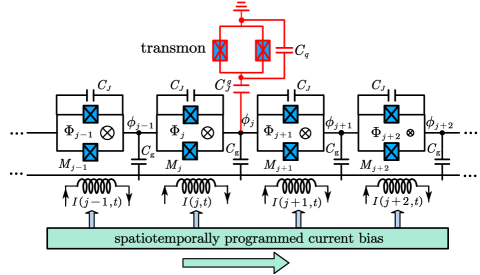
Figure 1: The proposed setup where a SQUID-metamaterial waveguide couples to a transmon qubit. The artificial waveguide is composed by a SQUID array, which impedance is modulated by a programmed current bias in each unit structure. The current signal $I(j,t)$ changing with both SQUID’s positions $j$ and time $t$ will spatiotemporally modulated the flux $\Phi_{j}$ through each SQUID via mutual inductance $M_{j}$. The Josephson (ground) capacitance of each SQUID is denoted as $C_{J}$ ($C_{0}$). The node flux $\phi_{j}$ at position $j$ follows the Kirchhoff current relation in Eq. (2). A transmon qubit, which is in the form of a split junction with Josephson capacitance $C_{q}$, interacts with the waveguide at position $x_{0}=0$ via a coupling capacitance $C_{J}^{g}$.

As shown in Fig 1, we consider that the Josephson-metamaterial waveguide is composed by a SQUID array which allows microwave photons propagating along it Weissl (2014); et al. (2015); Krupko and Nguyen (2018). Each node is connected to the ground with a capacitance $C_{g}$. Two neighbor sites are separated with distance $d_{0}$. The SQUID can be viewed as a nonlinear Josephson inductance $L_{j}$ in parallel with a capacitance $C_{J}$. A series of current biases which can be programmed with external signals will produce site-dependent flux $\Phi_{j}$ via mutual inductance $M_{j}$. The relation between $L_{j}$ and $\Phi_{j}$ is given by Wallquist et al. (2006); Sandberg and et al. (2008); Eichler and Wallraff (2014); Pogorzalek and Fedorov (2017); Eichler and Petta (2018); Wang et al. (2021)

$$L_{j}=\frac{L_{0}}{\cos\left|\frac{\pi\Phi_{j}}{\Phi_{0}}\right|},\quad L_{0}=\frac{\Phi_{0}^{2}}{8\pi^{2}E_{s0}},$$ (1)

where $E_{s0}$ is the Josephson energy of one junction. Defining the node flux as $\phi_{j}$, we obtain the following Kirchhoff current equation for the SQUID chain Weissl (2014); et al. (2015)

$$\frac{\phi_{j+1}-\phi_{j}}{L_{j+1}}-\frac{\phi_{j}-\phi_{j-1}}{L_{j}}=$$

$$C_{g}\ddot{\phi}_{j}+C_{J}\left(\ddot{\phi}_{j}-\ddot{\phi}_{j-1}\right)-C_{J}\left(\ddot{\phi}_{j+1}-\ddot{\phi}_{j}\right).$$ (2)

We assume that the current biases are composed of a static part and a time-dependent part, respectively. That is,

$$\Phi_{j}(t)=M_{j}[I_{0}+\delta If(j,t)],$$ (3)

where $I_{0}$ ($\delta I$) is the amplitude of the DC (AC) part satisfying $\delta If(j,t)\ll I_{0}$. We define $G_{j}(t)$ as

$$G_{j}(t)=\frac{1}{L_{j}(t)}=\frac{1}{L_{0}}\left[\alpha_{0}+\delta\alpha f(j,t)\right],$$ (4)

where

$$\alpha_{0}=\cos\left(\frac{\pi M_{j}I_{0}}{\Phi_{0}}\right),$$ (5)

$$\delta\alpha=-\sin\left(\frac{\pi M_{j}I_{0}}{\Phi_{0}}\right)\frac{\pi M_{j}\delta I}{\Phi_{0}}.$$ (6)

As discussed in Appendix A, given that $\phi_{j}$ varies slowly in the length scale $d_{0}$ (i.e., long wavelength limit), the difference Equation (2) can be written in a quasi-continuous form. Defining $c_{g}=C_{g}/d_{0}$ ($c_{J}=C_{J}/d_{0}$) as the ground (Josephson) capacitance per unit length, the wave function in the quasi-continuous limit becomes Wang et al. (2021)

$$c_{g}\frac{\partial^{2}\phi(x,t)}{\partial t^{2}}=c_{J}d_{0}^{2}\frac{\partial^{4}\phi(x,t)}{\partial t^{2}\partial x^{2}}+\frac{\partial}{\partial x}\left[g(x,t)\frac{\partial\phi(x,t)}{\partial x}\right],$$ (7)

where $g(x,t)$ is expressed as

$$g(x,t)=\frac{1}{l_{J}}\left[\alpha_{0}+\delta\alpha f(x,t)\right],\quad l_{J}=\frac{L_{0}}{d_{0}},$$ (8)

with $l_{J}$ being the Josephson inductance per unit length. The spatiotemporal modulation signal is encoded in $f(x,t)$. When $C_{J}=0$, Eq. (7) is simplified as a transmission-line equation in which the impedance is modulated by a space-time-varying wave. A non-zero Josephson capacitance $c_{J}$ will entangle both spatial and temporal differentials together, which will produce a nonlinear dispersion for the SQUID waveguide. In Appendix A and following discussions, we discuss its effects and give the conditions where $c_{J}$ can be neglected.

$d_{0}$	$C_{g}$	$C_{J}$	$L_{0}$	$\alpha$	$\delta\alpha/\alpha$	$k_{d}/(2\pi)$	$v_{0}$	$v_{d}$
$1~{}\mu\text{m}$	0.2 fF	100 fF	0.2 nH	0.3	$0.15$	$0.25\times 10^{4}\text{m}^{-1}$	$2.7\times 10^{6}~{}\text{m/s}$	$(0.05\sim 0.08)v_{0}$

Table 1: The parameters adopted for calculating the spectrum of the modulated SQUID-metamaterial waveguide.

The eigen-wave functions of the field are obtained by adopting a generalized Bloch-Floquet expansion Slater (1958); Trainiti and Ruzzene (2016); Calajó et al. (2019)

$$\phi_{lk}(x,t)=e^{i(\widetilde{\omega}_{l}(k)t-kx)}\sum_{n=-\infty}^{n=\infty}u_{ln}(k)e^{in(\Omega_{d}t-k_{d}x)},$$ (9)

where $\widetilde{\omega}_{l}$ is the quasi-energy of the $l$th band, and $k$ is the wave number. For convenience, we define $v_{0}=1/\sqrt{l_{J}c_{g}}$ as the propagation velocity of the static SQUID metamaterial waveguide without modulation. Now we consider the bias current $g(x,t)$ varying periodically in both space and time, i.e.,

$$g(x,t)=g(x+\lambda_{d},t+T_{d}).$$

The simplest modulation signal is a travelling wave, and in this work we adopt $f(x,t)$ as

$$f(x,t)=\cos{(\Omega_{d}t-k_{d}x)}.$$ (10)

The phase velocity is $v_{d}=\Omega_{d}/k_{d}$ with $k_{d}=2\pi/\lambda_{d}$ ($\Omega_{d}=2\pi/T_{d}$) being the wave number (angular frequency). By substituting Eq. (9) into Eq. (7), the dispersion relation is obtained by solving a quadratic eigenvalue problem Trainiti and Ruzzene (2016). Detailed derivations can be found in Appendix A.

According to the experiments in Refs. et al. (2015); Krupko and Nguyen (2018); et al. (2019c), we list the parameters adopted for our numerical simulation in Table 1. Although we can employ the generalized Floquet form in Eq. (9) to derive the spectrum, it does not mean that all kinds of modulation waves can produce stable eigenmodes in the SQUID transmission line. As discussed in Ref. Cassedy (1967), when the modulation velocity $v_{d}$ is faster than $v_{0}$, the eigenfrequencies become complex, indicating that the oscillations are time-growing and unstable. The high-speed modulation signal can be employed for conversing vacuum fluctuations into photons, which is analog to the Hawking effect in a gravitational system Nation et al. (2009); Blencowe and Wang (2020).

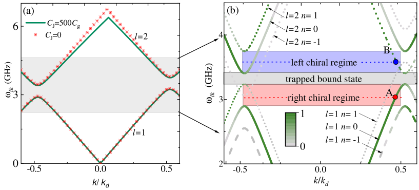
Figure 2: (a) Dispersion relation between quasi-energy $\omega_{l}(k)$ and wave number $k$ for $C_{J}=500C_{g}$ and $C_{J}=0$, respectively. The enlarged plot of the band gap [the area inside the box in (a)] is depicted in (b). The dispersion relations for different Floquet orders $\{l,n\}$ [corresponding to time-dependent part in Eq. (9)] are shown. The distribution ratio of each Floquet order is mapped with colors. The nontrivial spectra can be divided into three parts. In the red (blue) area, the microwave photons propagate into the right (left) direction; In the grey area, the microwave photon will be localized due to no propagating modes.

In this study, we focus on the parameter regimes with $v_{d}\ll v_{0}$. The first Brillouin zone (BZ) is limited within $k\in(-0.5k_{d},0.5k_{d}]$. There will be Brillouin-scattering processes between modes $k$ and $k+k_{d}$ (which are wave numbers for the eigenmodes of the static waveguide) due to the conservation of momentum. Additionally, the conservation of energy also requires $\omega_{l}(k)\pm\Omega_{d}\simeq\omega_{l}(k+k_{d})$. Since $\Omega_{d}$ is much smaller than $\omega_{l}$ at $k=k_{d}/2$, the modes around $k\simeq\pm 0.5k_{d}$ will interact with each other. The interactions between modes produces two band gaps, which is similar to the appearance of an anti-crossing point in a two-coupled-mode system.

We assume that the waveguide is long enough ($L\rightarrow\infty$) to support the microwave photons propagating without reflection. By quantizing the field, the root-mean-square voltage operator $\hat{V}(x,t)$ is written as Gu et al. (2017)

$$\hat{V}(x,t)\simeq-i\sum_{lk}\sqrt{\frac{\hbar\widetilde{\omega}_{l}(k)}{2C_{t}}}\left[\phi_{lk}^{*}(x,t)a_{lk}-\phi_{lk}(x,t)a^{\dagger}_{lk}\right],$$ (11)

where $C_{t}=Lc_{g}$ is the total capacitance of the waveguide, and $a_{lk}$ ($a_{lk}^{\dagger}$) is the annihilation (creation) operator for mode $k$ in the $l$th quasi-energy band. We numerically plot $\omega_{l}(k)$ changing with wave number $k$ in Fig. 2(a) by adopting parameters in Table 1. We find that an energy gap emerges between the two lowest bands in the first BZ $(-0.5k_{d},0.5k_{d}]$. As discussed in Appendix A, under the following condition

$$\sqrt{\frac{c_{J}}{c_{g}}}\ll\frac{1}{\left(k+nk_{d}\right)d_{0}},$$ (12)

the nonlinear effect led by $c_{J}$ can be neglected. By adopting the parameters in Table 1, one finds that $k_{d}d_{0}=0.25\times 10^{-2}\ll 1$. According to Eq. (12), even when $C_{J}=500C_{g}$, the nonlinear effect of Josephson capacitance is not apparent, and the dispersion relation is quite close to that with $C_{J}=0$.

Equation (9) shows that the time-dependent part of $\phi_{lk}(x,t)$ depends on both band index $l$ and Floquet order $n$, and the distribution ratio of the $n$th Floquet order is $|u_{ln}(k)|^{2}$ (note that $\sum_{n}|u_{ln}(k)|^{2}=1$) for a certain mode $lk$. Since the modulation signal $g(x,t)$ can be viewed as a perturbation, $|u_{ln}(k)|$ decreases quickly with $n$ according to our numerical calculations. For the parameters in Table 1, it is accurate enough to consider $n=0,\pm 1$, and the corresponding dispersion relation is plotted in Fig. 2(b) with $|u_{ln}(k)|^{2}$ being mapped with colors.

The modulation signal $g(x,t)$ propagates unidirectionally (rather than a standing wave carrying opposite momentums $\pm k_{d}$), which will open two asymmetric energy gaps located around $k=\pm 0.5k_{d}$ (see Fig. 2). Consequently, the unconventional spectrum regime in Fig. 2 can be divided into three parts. The gray area between two quasi-energy bands, where $|u_{ln}(k)|\simeq 0$ are valid for all Floquet orders $\{l,n\}$, is the conventional band gap with no propagating mode in the waveguide. In red (blue) area where point A (B) is located, the dispersion relation is asymmetric and the Floquet order $\{l=1,n=0\}$ ($\{l=2,n=-1\}$) possesses the highest distribution ratio $|u_{ln}(k)|$. In these two regimes microwave photons propagate unidirectionally, which will be discussed below by considering a superconducting qubit interacting with this metamaterial waveguide.

III Chiral emission of superconducting qubits

III.1 Interaction Hamiltonian of metamaterial waveguide coupling to superconducting qubits

As depicted in Fig. 1(a), we first consider the simplest QED setup where a transmon qubit interacts with the metamaterial waveguide via a coupling capacitance $C^{g}_{J}$ at $x_{0}$. The transom qubit is composed by two identical junctions which form a SQUID loop, and its Hamiltonian is written as Blais et al. (2004); Koch et al. (2007)

$$H_{\text{q}}=4E_{C}(\hat{n}-n_{g})^{2}-2E^{q}_{J}\cos\!\left(\frac{\pi\Phi_{\text{q}}}{\Phi_{0}}\right)\cos{\hat{\phi}},$$ (13)

where $\hat{n}$ ($\hat{\phi}$) is the charge (phase) operator of the transmon, $C_{\Sigma}=C^{q}_{J}+C_{q}$ with $C_{q}$ being the Josephson capacitance, and $E^{q}_{J}$ ($E_{C}=e^{2}/(2C_{\Sigma})$) is the Josephson (charging) energy of the junction. The interaction Hamiltonian between the transmon and the waveguide is written as Koch et al. (2007)

$$H_{\text{int}}=2e\frac{C^{q}_{J}}{C_{\Sigma}}\hat{V}(x,t)\hat{n}.$$ (14)

In the limit $E_{C}\ll E_{J}^{q}$, the transmon can be viewed as a Duffing nonlinear oscillator. Given that only the two lowest energy levels are considered, $H_{\text{q}}$ can be approximately written as Koch et al. (2007)

$$H_{\text{q}}=\frac{1}{2}\omega_{q}\sigma_{z},\qquad\omega_{q}=4\sqrt{E_{C}E^{q}_{J}}-E_{C},$$ (15)

where the charge operator is

$$\hat{n}=-i\sqrt[4]{\frac{E_{J}^{q}}{4E_{C}}}\frac{\sigma_{-}-\sigma_{+}}{\sqrt{2}}.$$ (16)

In the rotating frame of $\omega_{q}\sigma_{z}/2+\sum_{lk}\hbar\widetilde{\omega}_{l}(k)a^{\dagger}_{lk}a_{lk}$ and by adopting the rotating-wave approximation, we rewrite $H_{\text{int}}$ as

$$H_{\text{int}} = \hbar g_{0}\sum_{lk}e^{i\omega_{q}t}\sigma_{+}a_{lk}\phi^{*}_{lk}(x_{c},t)+\text{H.c.}$$ (17)

$$= \hbar\sum_{lk}g_{lk}\sigma_{+}a_{lk}e^{i\omega_{q}t}$$

$$\times \left[e^{-i\widetilde{\omega}_{l}(k)t}\sum_{n=-\infty}^{n=\infty}u^{*}_{ln}(k)e^{-in\Omega_{d}t}\right]+\text{H.c.},$$

where the coupling position is set at $x_{0}=0$ without loss of generality, and $g_{lk}$ is the coupling strength which is derived as

$$g_{lk}=\sqrt{2}\frac{eC^{q}_{J}}{\hbar C_{\Sigma}}\sqrt[4]{\frac{E_{J}^{q}}{4E_{C}}}\sqrt{\frac{\hbar\widetilde{\omega}_{l}(k)}{2C_{t}}}.$$ (18)

Here we take the transmon as an example. As discussed in experimental work in Refs. Rastelli and Pop (2018); et al. (2019c); Wang et al. (2021), the SQUID-metamaterial waveguide can also interact with a flux or charge qubit, and all these circuit-QED setups can be employed to demonstrate the unconventional emission behaviors discussed in this work.

III.2 Chiral emission in Markovian regime

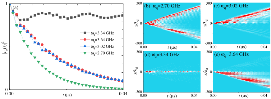
Figure 3: (a) The time-dependent evolution $|c_{e}(t)|^{2}$ for different transmon frequencies, and the field distributions are shown in (b-e), respectively. The corresponding relations are (b) bidirectional emission $\rightarrow\omega_{q}=2.70~{}\text{GHz}$, (c) right emission $\rightarrow\omega_{q}=3.02~{}\text{GHz}$, (d) trapped bound state $\rightarrow\omega_{q}=3.34~{}\text{GHz}$ and (e) left emission $\rightarrow\omega_{q}=3.64~{}\text{GHz}$. The system’s parameters are adopted from Table 1 with $v_{d}=0.05v_{0}$.

Similar to the standard spontaneous emission process, the intensity of radiation field should be narrowly centered around the atomic transition frequency $\omega_{q}$. Therefore, by replacing $\widetilde{\omega}_{l}(k)$ in Eq. (18) with $\omega_{q}$, $g_{lk}$ becomes mode-independent, i.e., $g_{lk}\simeq g_{0}$. We assume that a single excitation is initially in the transmon qubit, while the waveguide is in vacuum state $|0\rangle$. Due to the conservation of excitation number for the Hamiltonian in Eq. (17), the system’s state at time $t$ can be expressed in the single-excitation subspace as

$$|\Psi(t)\rangle=c_{e}(t)|e,0\rangle+\sum_{l,k}c_{lk}(t)|g,1_{lk}\rangle,$$ (19)

where $|1_{lk}\rangle$ represents a single photon being excited in mode $a_{lk}$. The evolution governed by $H_{\text{int}}$ can be derived from the following coupled differential equations

$$\frac{\partial c_{e}(t)}{\partial t} = -ig_{0}\sum_{lkn}c_{lk}u_{ln}(k)e^{[i\Delta_{l}(k)-in\Omega_{d}]t},$$ (20)

$$\frac{\partial c_{lk}(t)}{\partial t} = -ig_{0}c_{e}(t)e^{-i\Delta_{l}(k)t}\sum_{n}u_{ln}^{*}(k)e^{in\Omega_{d}t},$$ (21)

where $\Delta_{l}(k)=\omega_{q}-\widetilde{\omega}_{l}(k)$ is the frequency detuning between the qubit and the mode $a_{lk}$. By substituting the integration form of Eq. (21) into Eq. (20), we obtain

$$\frac{\partial c_{e}(t)}{\partial t} = -g_{0}^{2}\int_{0}^{t}dt^{\prime}G(t,t^{\prime})c_{e}(t^{\prime}),$$ (22)

$$G(t,t^{\prime}) = \sum_{lknn^{\prime}}e^{-i(n-n^{\prime})\Omega_{d}t}u_{ln}(k)u_{ln^{\prime}}^{*}(k)e^{i[\Delta_{l}(k)-n\Omega_{d}](t-t^{\prime})},$$ (23)

where $G(t,t^{\prime})$ is the time-delay correlation function. Given that $n\neq n^{\prime}$, $e^{-i(n-n^{\prime})\Omega_{d}t}$ are fast oscillating terms, and their contributions to the evolution will be significantly suppressed when the decaying time scale is much longer than the oscillating period $\Omega_{d}^{-1}$. Under these conditions, we can only keep the resonant term $n=n^{\prime}$, which is similar to the rotating-wave approximation Calajó et al. (2019). Finally we obtain

$$G(t,t^{\prime}) = \sum_{lkn}|u_{ln}(k)|^{2}e^{i[\Delta_{l}(k)-n\Omega_{d}](t-t^{\prime})}$$ (24)

$$= \sum_{ln}\frac{L}{2\pi}\int dk|u_{ln}(k)|^{2}e^{i[\Delta_{l}(k)-n\Omega_{d}](t-t^{\prime})}.$$

In the emission spectrum, the intensity of the field will center at the modes satisfying the resonant condition

$$\Delta_{l}(k)-n\Omega_{d}=0,$$ (25)

which solutions of $k$ are denoted as $k_{ln}$. For example, in Fig. 2(b) for the frequency at the dashed position in the red regime, we mark the resonant positions (green dot $A$) for $\{l=1,n=0\}$. Around each $k_{ln}$, one can approximately derive the dispersion relation as

$$\Delta_{l}(k)=\Delta_{l}(k_{ln})+v_{ln}(k-k_{ln}),$$ (26)

where

$$v_{ln}=\frac{\partial\Delta_{l}(k_{ln})}{\partial k}\Big{|}_{k_{ln}}$$

is the group velocity. When the qubit transition frequency is far away from the band edges, $G(t,t^{\prime})$ can be written as

$$G(t,t^{\prime}) \simeq \sum_{ln}\frac{L}{2\pi}|u_{ln}(k_{ln})|^{2}\int_{-\infty}^{\infty}d(\delta k)e^{-iv_{ln}\delta k(t-t^{\prime})}$$ (27)

$$= \sum_{ln}\frac{L|u_{ln}(k_{ln})|^{2}}{|v_{ln}|}\delta(t-t^{\prime}).$$

The delta function in Eq. (27) is valid given that the bandwidth of the waveguide’s spectrum is approximately infinite compared with the interaction strength. By substituting Eq. (27) into Eq. (23), we obtain

$$\frac{\partial c_{e}(t)}{\partial t} = -\frac{\Gamma_{T}}{2}c_{e}(t),\quad\Gamma_{T}=(\Gamma_{R}+\Gamma_{L}),$$ (28)

$$\Gamma_{R(L)} = \Gamma_{0}\sum_{ln}|u_{ln}(k_{ln})|^{2}\Theta(\pm v_{ln}),$$ (29)

where $\Theta(x)$ is the Heaviside step function, $\Gamma_{R(L)}$ corresponds to the decay rate to the right (left) hand of the waveguide, and $\Gamma_{0}$ is the characteristic decay rate for the qubit which is derived as

$$\Gamma_{0}=\frac{g_{0}^{2}L}{v_{0}}=\frac{1}{\hbar v_{J}}\left(\frac{eC^{q}_{J}}{C_{\Sigma}}\right)^{2}\sqrt[2]{\frac{E_{J}^{q}}{4E_{C}}}\frac{\omega_{q}}{2c_{g}}.$$ (30)

In the single-excitation subspace expressed in Eq. (19), the photonic wave function in real space is Scully and Zubairy (1997)

$$\psi_{\gamma}(x,t)=\sum_{lkn}c_{lk}(t)e^{ikx}u^{*}_{ln}(k)e^{-in(\Omega_{d}t-k_{d}x)}.$$ (31)

The photonic energy decaying into the right (left) hand side is expressed as

$$\Phi_{R/L}=\left|\int_{0}^{\pm\infty}|\psi_{\gamma}(x^{\prime},t)|^{2}dx^{\prime}\right|,\quad t\rightarrow\infty.$$ (32)

By neglecting the local decoherence and dephasing of the transmon, the chiral factor is defined as Lodahl et al. (2017)

$$\beta_{\pm}=\frac{\Gamma_{R(L)}}{\Gamma_{R}+\Gamma_{L}}=\frac{\Phi_{R(L)}}{\Phi_{R}+\Phi_{L}}.$$ (33)

As indicated in Eq. (29), the directional emission rates depend on both distributions ratios $|u_{ln}(k_{ln})|$ and group velocities $v_{ln}$. For example, given that the qubit frequency lies in the red regime of Fig. 2(b), the Floquet order $\{l=1,n=0\}$ has the largest $|u_{ln}(k_{ln})|$ (see point A), and the corresponding $v_{ln}$ is positive. Consequently, the photon will be chirally emitted to the right direction. In the blue regime (point B), the emission chirality will be reversed. Below we will numerically discuss the emission behaviors in different frequency regimes.

III.3 Numerical discussions

The chiral spontaneous emission process can well be described by the master equation, which however discards much information due to a lot of approximations. For example, master equation cannot describe the directional field distribution and Non-Markovian dynamics led by band-edge effects. To avoid those problems, we numerically simulate the unitary evolution governed by Hamiltonian in Eq. (17) by discretising the modes of the modulated waveguide in the momentum space. The photonic field in the waveguide is recovered from Eq. (31). The details about numerical methods are presented in Appendix B.

By changing the transmon’s frequency, we plot the evolutions of $|c_{e}(t)|^{2}$ in Fig. 3(a). When $\omega_{q}$ is in the conventional dispersion regime [$\omega_{q}/(2\pi)=2.70~{}\text{GHz}$], the transmon exponentially decays its energy, and the photonic field is symmetrically emitted into both left and right side [see Fig. 3(b)]. In the right chiral regime with $\omega_{q}/(2\pi)=3.02~{}\text{GHz}$ [see red horizontal line in Fig. 2(b)], the solutions for Eq. (25) correspond to the intersection points with the dispersion curves of different Floquet orders. The intersection point A with the Floquet order $\{l=1,n=0\}$ has the largest distribution ratio $|u_{ln}(k)|\simeq 1$, while the other $|u_{ln}(k)|$ are of extremely low amplitudes. The group velocity for point A is positive. Therefore, the transmon will chirally emit photons into the right part of the waveguide, as indicated by Eq. (29). Similarly, when transmon frequency is in the blue regime, most of the emitted photonic field will distribute on its left hand side. The chiral field distributions changing with time are shown in Fig. 3(c, e), respectively. Moreover, the chiral factor is about $\beta_{\pm}\simeq 0.95$, indicating that this SQUID-metamaterial waveguide can be implemented as a well-performance directional quantum bus.

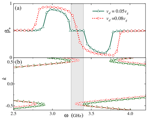
Figure 4: (a) The chiral factor $\beta_{+}$ changes with $\omega_{q}$ by setting modulation group velocities as $v_{d}=0.05v_{g}$ and $v_{d}=0.08v_{g}$. (b) The corresponding dispersion relation of the quasi-energy $\omega_{l}(k)$ of the waveguide.

When the qubit frequency lies within the band gap [the gray regime in Fig. 2(b)], the distribution ratios for all Floquet orders are around zero, i.e., $|u_{ln}(k)|\simeq 0$, indicating that there is no resonant mode which can lead to exponential decay of the transmon qubit. In this scenario, the transmon only decays its partial energy into the waveguide [see Fig. 3(a) for $\omega_{q}/(2\pi)=3.34~{}\text{GHz}$], and the field is localized around the coupling position without propagating outside, as shown Fig. 3(d)]. This unconventional evolution can be understood from Fig. 2(b): in the gray regime, the coefficients of all the Floquet orders are around zero, i.e., $|u_{ln}(k_{ln})|\simeq 0$. Due to no resonant mode, only the modes which are of large detuning will contribute significantly to the dynamics. Those modes are of large density due to band edge effects, and the field will be localized in the form of bound state. The scenario is akin to an emitter being prevented from spontaneous emission when it is trapped by the band gap of a photonic crystal waveguide Goban and et al. (2014); González-Tudela and et al. (2015); Douglas et al. (2016).

In this proposal the modulation signal is programmable. Therefore, the dispersion relation of the waveguide can be tailed freely, which enables us to control the qubit dynamics on demand. For example, given that the modulation phase velocity $v_{d}$ is switched oppositely, the chiral direction with a certain qubit frequency is also reversed. In Fig. 4(a), we plot the chiral factor $\beta_{+}$ changing with transmon frequency by setting modulation velocity as $v_{d}=0.05v_{g}$ and $v_{d}=0.08v_{g}$, respectively. When $v_{d}=0.05v_{g}$, the quasi-energy band $l=1$ and $l=2$ are separated by a finite band gap [see gray area in Fig. 2(b)]. The gap leads to the trapped bound state when the qubit frequency lies within this regime [see Fig. 3(d)]. As discussed in Ref. Trainiti and Ruzzene (2016), when increasing the modulation velocity, the gap disappears, which can be found from the dispersion relation for $v_{d}=0.08v_{g}$ depicted in Fig. 4(b). The chirality will be smoothly switched from left to right without any gaps when increasing the qubit frequency. With a larger $v_{d}$ the chirality is enhanced and the directional bandwidth becomes wider [see Fig. 4(a)], which is due to that the Brillouin-scattering process emerges between the modes with a large energy difference. However, as discussed in Refs. Trainiti and Ruzzene (2016); Cassedy (1967), when the modulation velocity $v_{d}$ is comparable to $v_{0}$, the waveguide’s eigenfrequencies become complex, indicating the field is time-growing and unstable. Due to this, the modulation velocity $v_{d}$ should be much smaller than $v_{0}$ to avoid the unstable phenomena emerging in the whole setup.

IV Chiral photon flow between two quantum nodes

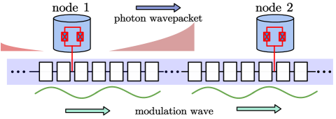
Figure 5: By mediating remote nodes, the metamaterial waveguide can work as a common quantum bus in a chiral quantum network. The metamaterial waveguide is placed in a tube which is below the superconducting temperature (see experiments in in Ref. Magnard et al. (2020)). To suppress the thermal microwave noise, each node is placed in a dilution refrigerator which temperature is around $T\sim 10~{}\text{mk}$.

By considering multiple nodes interacting with the same metamaterial waveguide, our proposal in Fig. 1 can be extended as a chiral quantum network. The schematic cascaded network is depicted in Fig. 5, where nodes are placed in separated dilution refrigerators with temperature $\sim 10~{}\text{mK}$ to suppress the thermal noise. As discussed in Ref. Magnard et al. (2020), the metamaterial waveguide can be inside a multi-sleeve tube which is below the superconducting critical temperature. This experimental method allows to connect transmons located in different cryogenic refrigerators. Given that the transmons’ frequencies are identical, the interaction Hamiltonian can be written as

$$H_{\text{int},2}=\hbar g_{0}\sum_{i}\sum_{lk}e^{i\omega_{q}t}\sigma_{i}^{+}a_{lk}\phi^{*}_{lk}(x_{i},t)+\text{H.c.},$$ (34)

where $x_{i}$ is the coupling position of the $i$th node. As discussed in Appendix C, we can derive the cascaded master equation for multiple nodes by tracing over the waveguide’s freedoms. Taking that two transmons chirally decay/absorb the right propagating photons for example, the evolution is governed by

$$\dot{\rho}_{s}(t) = -iH_{\text{eff}}\rho_{s}+i\rho_{s}H^{\dagger}_{\text{eff}}+\mathcal{L}\rho_{s}\mathcal{L}^{\dagger},$$

$$H_{\text{eff}} = -i\sum_{i}\frac{\Gamma_{R}}{2}\sigma_{i}^{+}\sigma_{i}^{-}-i\sum_{i>j}\Gamma_{R}\sigma_{i}^{+}\sigma_{j}^{-}.$$ (35)

where $\rho_{s}$ is the reduced density matrix operator for two transmons, $\Gamma_{R}$ is the decay rate to the right side, and $\mathcal{L}=\sqrt{\Gamma_{R}}(\sigma_{1}^{-}+\sigma_{2}^{-})$ is the collective jump operator. The last term in $H_{\text{eff}}$ is unique to the cascaded quantum system, and describes the irreversible process that a photon emitted by transmon $j$ will be reabsorbed by transmon $i$, while the information back flow is prevented Lodahl et al. (2017). As discussed in Appendix C, when deriving the cascaded master Eq. (35), we assume that the propagating time $\tau_{ij}=(x_{i}-x_{j})/v_{ln}$ between two nodes is much smaller than the decaying time scale $\Gamma_{R}^{-1}$. Therefore, we can adopt the Markovian approximation $t-\tau\simeq t$, and the evolution becomes independent of time delay. This approximation is valid only when the separation distance $x_{ij}$ is much shorter than the wavepacket’s size.

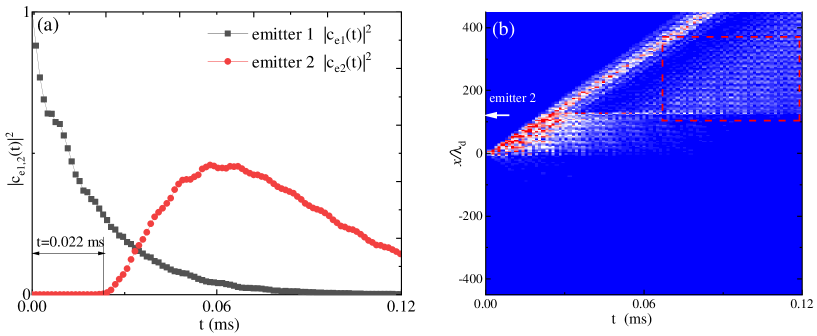
Figure 6: (a) The directional photon flow from transmon 1 ($x=0$) to transmon 2 ($x=125k_{d}$). Due to the time-delay effect, transmon 2 is excited with a retardation time $t=x_{12}/v_{0}$. (b) The field distribution along the waveguide changes with $t$. At $x=125k_{d}$, the emitted photon is scattered by transmon 2. Due to directional transport, the scattered field only propagates into the right direction. The adopted parameters are the same with those in Fig. 3(c).

In cascaded master equation (35), the evolution information, such as the field distribution and time-decay effects, has been discarded due to taking a trace over waveguide’s freedoms. To proceed beyond those limitations, our simulation is based on the unitary evolution governed by the Hamiltonian in (34), which can well describe the time-delay effects Wang and Li (2022). Numerical details can be found in Appendix B. In Fig. 6(a), by assuming a single excitation initially in transmon 1, we plot the evolution of two transmons with a separation distance $x_{2}-x_{1}=125\lambda_{d}$. At the frequency adopted in Fig. 3(c), the group velocity is around $v_{ln}\simeq 0.83v_{0}$, which is slower than $v_{0}$ due to the nonlinear dispersion relation around the band edge. Consequently the wave front arriving at transmon 2 is calculated as $\tau_{ij}=125\lambda_{d}/0.83v_{0}\simeq 0.022\text{ms}$ [see Fig. 6(a)]. The field distribution $|\psi_{\gamma}(x,t)|^{2}$ is depicted in Fig. 6(b), where one finds that the photon emitted by transmon 1 propagates unidirectionally, and the field absorbed by transmon 2 (inside the box) is aslo re-emitted to the right side. Due to no photonic energy back flow, transmon $1$ will not be re-excited. Those numerical results show that our proposal can behave as a well-performed cascaded quantum network.

V Summary and outlooks

In this work, we propose how to employ the Josephson array as chiral metamaterial waveguide for circuit-QED. The waveguide is in the form of SQUID chain which impedance is modulated with bias currents. When the bias signals are programmed as travelling waves, the symmetry between the left and right propagating modes is broken due to the Brillouin-scattering process. We also discuss the quantum optical phenomena by considering superconducting qubits coupling to this metamaterial waveguide. By applying the optimized modulating parameters, the qubit will emit photons unidirectionally, and chiral factor can approach 1. Last we extend our proposal as a multi-node quantum network, and demonstrate that the chiral transport between remote nodes can be realized. Compared with routing microwave photons unidirectionally with the bulky ferrite circulators, our proposal does not require strong magnetic field, and the direction can be freely tuned by the programmed bias signals.

Note that we only focus on slow travelling waves to modulate the SQUID-chain’s impedance. Exploring other modulating parameters or forms, such as standing-wave modulations and pulses with different shapes, might allow us to observe more intriguing QED phenomena in this metamaterial platform. As discussed in experimental studies in Refs. et al. (2019c); Planat et al. (2020), the SQUID number in a single metamaterial waveguide can be around $10^{3}\simeq 10^{4}$, indicating that our proposal is within the capability of current technology. We hope that our work can inspire more efforts being devoted to exploiting SQUID metamaterials for controlling microwave photons in SQC setups.

VI Acknowledgments

The quantum dynamical simulations are based on open source code QuTiP Johansson et al. (2012, 2013). X.W. is supported by the National Natural Science Foundation of China (NSFC) (Grant No. 12174303 and No. 11804270), and China Postdoctoral Science Foundation No. 2018M631136. W.X.L. was supported by the Natural Science Foundation of Henan Province (No. 222300420233). H.R.L. is supported by the National Natural Science Foundation of China (NSFC) (Grant No.11774284).

APPENDICES

Appendix A Deriving the dispersion relation of the modulated SQUID-metamaterial waveguide

We start from the left side of Eq. (2), i.e., the difference terms related to time-dependent inductance $L_{j}(t)$. To derive the corresponding quasi-continuous differential form, we first rewrite it as

$$\frac{\phi_{j}-\phi_{j-1}}{L_{j}(t)}-\frac{\phi_{j+1}-\phi_{j}}{L_{j+1}(t)}=\frac{\phi_{j}-\phi_{j-1}}{L_{j}(t)}-\frac{\phi_{j+1}-\phi_{j}}{L_{j}(t)}+\frac{\phi_{j+1}-\phi_{j}}{L_{j}(t)}-\frac{\phi_{j+1}-\phi_{j}}{L_{j+1}(t)}.$$ (A1)

In this work we assume that each SQUID’s size is much smaller than wavelengths of both modulation wave and microwave photons. Therefore, we replace $\phi_{j}(t)\rightarrow\phi(x,t)$ and $f(j,t)\rightarrow f(x,t)$. Note that $G_{j}(t)$ becomes

$$G(x,t)=\frac{1}{L_{0}}\left[\alpha_{0}+\delta\alpha f(x,t)\right].$$ (A2)

By replacing $x=id_{0}$, Eq. (A1) is changed as

$$\frac{\phi_{j}-\phi_{j-1}}{L_{j}(t)}-\frac{\phi_{j+1}-\phi_{j}}{L_{j}(t)}+\frac{\phi_{j+1}-\phi_{j}}{L_{j}(t)}-\frac{\phi_{j+1}-\phi_{j}}{L_{j+1}(t)}=-G(x,t)\frac{\partial^{2}\phi(x,t)}{\partial x^{2}}d_{0}^{2}-\frac{\partial G(x,t)}{\partial x}\frac{\partial\phi(x,t)}{\partial x}d_{0}^{2}.$$ (A3)

Similarly, the left side in Eq. (2) which contains capacitance terms can also be written in quasi-continuous differential form. Finally, the nonlinear wave function of the modulated SQUID waveguide is derived as

$$C_{g}\frac{\partial^{2}\phi(x,t)}{\partial t^{2}}-C_{J}\frac{\partial^{4}\phi(x,t)}{\partial t^{2}\partial x^{2}}d_{0}^{2}=G(x,t)\frac{\partial^{2}\phi(x,t)}{\partial x^{2}}d_{0}^{2}+\frac{\partial G(x,t)}{\partial x}\frac{\partial\phi(x,t)}{\partial x}d_{0}^{2},$$ (A4)

which is equivalent to the form in Eq. (7).

Given that the modulation is of the travelling wave form, one can decompose the wave function in Eq. (2) as a matrix form by employing the orthogonal relations. The dispersion relation is obtained by solving the following quadratic eigenvalue problem

$$\left[\omega_{l}^{2}(k)\hat{M}_{2}+\omega_{l}(k)\hat{M}_{1}+\hat{M}_{0}\right]\hat{U}(k)=0,$$ (A5)

where $M_{1,2}$ are diagonal matrices and expressed as

$$\hat{M}_{2}=\text{diag}\left[...,-c_{J}(d_{0})^{2}\left(k+nk_{d}\right)^{2}-c_{g},...\right],$$ (A6)

$$\hat{M}_{1}=\text{diag}\left[...,-2n\Omega_{d}[c_{J}(d_{0})^{2}\left(k+nk_{d}\right)^{2}+c_{g}],...\right].$$ (A7)

The matrix $\hat{M}_{0}$ is

$$\hat{M}_{0} = \left(\begin{matrix}\ddots&\ddots&\ddots&0&0&0&\vdots\\ ...&T_{n-1,n-2}&T_{n-1,n-1}&T_{n-1,n}&0&0&...\\ ...&0&T_{n,n-1}&T_{n,n}&T_{n,n+1}&0&...\\ ...&0&0&T_{n+1,n}&T_{n+1,n+1}&T_{n+1,n+2}&0\\ \vdots&0&0&0&\ddots&\ddots&\ddots\end{matrix}\right),$$ (A8)

where

$$T_{n,n}=-\left(n\Omega_{d}\right)^{2}\left[c_{J}(d_{0})^{2}\left(k+nk_{d}\right)^{2}+c_{g}\right]+\frac{\alpha_{0}}{l_{0}}\left(k+nk_{d}\right)^{2},$$ (A9)

$$T_{n,n\pm 1}=\frac{\delta\alpha}{2l_{0}}\left\{\left(k+\left(n\pm 1\right)k_{d}\right)^{2}+\left(k+\left(n\pm 1\right)k_{d}\right)k_{d}\right\}.$$ (A10)

We find that the Josephson capacitance $c_{J}$ only appears in the diagonal terms of $\hat{M}_{0,1,2}$, from which on can easily find that $c_{J}$ can be neglected under the following condition

$$c_{J}(d_{0})^{2}\left(k+nk_{d}\right)^{2}\ll c_{g}.$$ (A11)

Further discussions of nonlinear dispersion led by $c_{J}$ can be found in Sec. II of the main text.

Appendix B Numerical methods for simulating spontaneous emission and non-Markovian dynamics

Although the master equation can well describe the spontaneous emission of emitters, the Born-Markovian approximation is not valid when the interaction strength is comparable to the band width of baths. Moreover, the information of emitted photons will be traced off when deriving the master equation. To avoid those, our simulation is based on the unitary evolution governed by the original Hamiltonian in Eqs. (17, 34). In the single-excitation subspace and taking for the case of two transmons for example, the system’s state is written as

$$|\psi(t)\rangle=\sum_{lk}c_{lk}(t)|g,g,1_{lk}\rangle+c_{e1}(t)|e,g,0\rangle+c_{e2}(t)|g,e,0\rangle,$$

where $|1_{lk}\rangle$ represents the single excitation being in $lk$th mode, and $|0\rangle$ corresponds to the waveguide in its vacuum. Since the Hamiltonian is expressed in momentum space, we first need to calculate waveguide’s eigen-frequencies and wavefunctions by employing the method presented in Appendix A. Next we discretise modes in the first BZ $k\in(-0.5k_{m},0.5k_{m}]$ with a large number $N$, which is equal to considering a waveguide with a length $L=N\lambda_{m}$. A similar method can be found in Ref Wang and Li (2022). In the single-excitation subspace, the Hamiltonian in Eq. (17) [Eq. (34)] can be mapped into a matrix with dimension $N+1$ ($N+2$) when the system contains a single emitter (two emitters). Taking two emitters ($Q=2$) for example, the corresponding matrix is written as

$$H_{\text{int}}=\left[\begin{matrix}w_{lk_{1}}&0&...&0&g_{0}\phi_{lk_{1}}(x_{1},t)&g_{0}\phi_{lk_{1}}(x_{2},t)\\ 0&w_{lk_{2}}&\ddots&...&g_{0}\phi_{lk_{2}}(x_{1},t)&g_{0}\phi_{lk_{2}}(x_{2},t)\\ \vdots&\ddots&...&0&\vdots&\vdots\\ 0&...&0&w_{lk_{N}}&g_{0}\phi_{lk_{N}}(x_{1},t)&g_{0}\phi_{lk_{N}}(x_{2},t)\\ g_{0}\phi^{*}_{lk_{1}}(x_{1},t)&g_{0}\phi^{*}_{lk_{2}}(x_{1},t)&...&g_{0}\phi^{*}_{lk_{N}}(x_{1},t)&w_{qa}&0\\ g_{0}\phi^{*}_{lk_{1}}(x_{2},t)&g_{0}\phi^{*}_{lk_{2}}(x_{2},t)&...&g_{0}\phi^{*}_{lk_{N}}(x_{2},t)&0&w_{qb}\\ \end{matrix}\right],$$ (B1)

where $\phi_{lk_{i}}(x_{j},t)$ is numerically obtained via methods in Appendix A. After obtaining the matrix form in Eq. (B1), we can numerically solve the evolution governed by the Schrödinger equation. At certain time $t=t_{i}$, the amplitude $c_{kl}(t)$ of each mode is recorded, and the field distribution can be recovered by substituting them into Eq. (31). Employing this method, we obtained both transmon’s and waveguide’s evolution shown in the main text.

Appendix C Cascaded master equation for multi-nodes system

In this part we will derive the cascaded master equation for multiple emitters mediated by the metamaterial waveguide. By expanding the Schrödinger equation to the second order, the evolution of the system is expressed as Scully and Zubairy (1997)

$$\dot{\rho}_{s}(t) = -\frac{i}{\hbar}\mathrm{Tr}_{R}{\left[H_{\mathrm{int},2}(t),\rho(t)\right]}-$$ (C2)

$$\!\frac{1}{\hbar^{2}}\mathrm{Tr}_{R}\int_{t_{0}}^{t}{\left[H_{\mathrm{int},2}(t),\left[H_{\mathrm{int},2}(t^{\prime}),\rho(t^{\prime})\right]\right]}dt^{\prime},$$

where $\rho$ ($\rho_{s}$) is the density matrix operator of the whole system (the emitters), and $\text{Tr}_{R}$ represents taking a trace over the waveguide’s freedoms. We assume that the waveguide is always approximately in its vacuum state. Therefore, the correlation relations for the waveguide’s modes satisfy $\langle a_{lk}\rangle=\langle a^{\dagger}_{lk}\rangle=\langle a^{\dagger}_{lk}a_{lk}\rangle=0$ and $\langle a_{lk}a^{\dagger}_{lk}\rangle=1$. By substituting those relations into Eq. (C2), we obtain

$$\dot{\rho}_{s}(t) = -g_{0}^{2}{\frac{L}{2\pi}}\sum_{i,j}\int_{t_{0}}^{t}dt^{\prime}A\left(x_{i},x_{j},t,t^{\prime}\right)$$ (C3)

$$\big{[}\sigma_{i}^{+}\sigma_{j}^{-}\rho_{s}(t^{\prime})-\sigma_{j}^{-}\rho_{s}(t^{\prime})\sigma_{i}^{+}\big{]}+\mathrm{H}.\mathrm{c}.,$$

where the correlation function $A\left(x_{i},x_{j},t,t^{\prime}\right)$ is defined as Calajó et al. (2019)

$$A\left(x_{i},x_{j},t,t^{\prime}\right)=e^{i\omega_{q}\left(t-t^{\prime}\right)}\sum_{lk}\phi_{lk}^{*}(x_{i},t)\phi_{lk}(x_{j},t)$$ (C4)

$$= \sum_{ln}|u_{ln}(k_{ln})|^{2}\int_{-\infty}^{\infty}{d}(\delta k)e^{-i\delta kv_{ln}\left[(t-t^{\prime})-\frac{x_{ij}}{v_{ln}}\right]}$$

$$= \sum_{ln}\frac{2\pi}{|v_{ln}|}|u_{ln}(k_{ln})|^{2}\delta\left[(t-t^{\prime})-\frac{x_{ij}}{v_{ln}}\right],$$

with $x_{ij}=x_{i}-x_{j}$ being the distance between two emitters. We have neglected the phase terms $e^{i\left(k_{ln}+k_{d}\right)\left(x_{i}-x_{j}\right)}$ in $A\left(x_{i},x_{j},t,t^{\prime}\right)$. Note that the integral regime is within $t^{\prime}\in[t_{0},t]$. Therefore, the $\delta$-funtion will produce non-zero value in Eq. (C3) only under the condition $t-x_{ij}/v_{ln}\leq t$. The delay-time $\tau_{ij}=x_{ij}/v_{ln}$ ($i\neq j$) corresponds to the propagating time between two separated emitters. When $x_{i}>x_{j}$ ($x_{i}<x_{j}$), the non-zero time-delay correlation is mediated by the right (left) propagating modes with $v_{ln}>0$ ($v_{ln}<0$). Given that $\tau_{ij}$ is much smaller than the time scale of spontaneous emission, we can replace $t-\tau\rightarrow t$, and Eq. (C3) is simplified as

$$\dot{\rho}_{s}(t) = \Big{\{}\frac{\Gamma_{R}+\Gamma_{L}}{2}\sum_{i}\big{[}\sigma_{i}^{+}\sigma_{i}^{-}\rho_{s}(t)-\sigma_{i}^{-}\rho_{s}(t)\sigma_{i}^{+}\big{]}$$ (C5)

$$-\sum_{i>j}\Gamma_{R}\big{[}\sigma_{i}^{+}\sigma_{j}^{-}\rho_{s}(t)-\sigma_{j}^{-}\rho_{s}(t)\sigma_{i}^{+}\big{]}+$$

$$\!\sum_{i<j}\Gamma_{L}\big{[}\sigma_{i}^{+}\sigma_{j}^{-}\rho_{s}(t)-\sigma_{j}^{-}\rho_{s}(t)\sigma_{i}^{+}\big{]}\Big{\}}\!+\!\mathrm{H}.\mathrm{c}.,$$

where $\Gamma_{R(L)}$ is the decay rate into right/left side, which are expressed in Eq. (29). In Eq. (C5) we have employed the properties of $\delta$-function

$$\int_{t_{0}}^{t}\delta\left(t-t^{\prime}-\frac{x_{ij}}{v_{ln}}\right)\rho_{s}(t^{\prime})dt^{\prime}=\left\{\begin{array}[]{lr}\frac{1}{2}\rho_{s}(t)\quad x_{ij}=0,\\ \rho_{s}(t)\quad x_{ij}/v_{ln}=0^{+},\\ 0\quad x_{ij}/v_{ln}<0.\end{array}\right.$$

When the chiral factor of the whole system approaches $\beta_{\pm}\simeq 1$, we obtain the cascaded master equation in the main text.

References

- Lamb and Retherford (1947) W. E. Lamb and R. C. Retherford, “Fine structure of the hydrogen atom by a microwave method,” Phys. Rev. 72, 241 (1947).
- Scully and Zubairy (1997) Marlan O. Scully and M. Suhail Zubairy, Quantum Optics (Cambridge University Press, 1997).
- Cohen-Tannoudji et al. (1998) C. Cohen-Tannoudji, J. Dupont-Roc, and G. Grynberg, Atom–Photon Interactions (Wiley, 1998).
- Walls and Milburn (2007) D. F. Walls and G. J. Milburn, Quantum Optics (Springer, Berlin, 2007).
- Clerk et al. (2010) A. A. Clerk, M. H. Devoret, S. M. Girvin, F. Marquardt, and R. J. Schoelkopf, “Introduction to quantum noise, measurement, and amplification,” Rev. Mod. Phys. 82, 1155 (2010).
- Buluta et al. (2011) I. Buluta, S. Ashhab, and F. Nori, “Natural and artificial atoms for quantum computation,” Rep. Prog. Phys. 74, 104401 (2011).
- Xiang et al. (2013) Z.-L. Xiang, S. Ashhab, J.-Q. You, and F. Nori, “Hybrid quantum circuits: Superconducting circuits interacting with other quantum systems,” Rev. Mod. Phys. 85, 623 (2013).
- Underwood et al. (2012) D. L. Underwood, W. E. Shanks, J. Koch, and A. A. Houck, “Low-disorder microwave cavity lattices for quantum simulation with photons,” Phys. Rev. A 86, 023837 (2012).
- Reiserer and Rempe (2015) A. Reiserer and G. Rempe, “Cavity-based quantum networks with single atoms and optical photons,” Rev. Mod. Phys. 87, 1379 (2015).
- Chang et al. (2018) D.-E. Chang, J. S. Douglas, A. González-Tudela, C.-L. Hung, and H. J. Kimble, “Colloquium: Quantum matter built from nanoscopic lattices of atoms and photons,” Rev. Mod. Phys. 90, 031002 (2018).
- Nakamura et al. (1999) Y. Nakamura, Y. A. Pashkin, and J. S. Tsai, “Coherent control of macroscopic quantum states in a single-Cooper-pair box,” Nature (London) 398, 786–788 (1999).
- Blais et al. (2004) A. Blais, R.-S. Huang, A. Wallraff, S. M. Girvin, and R. J. Schoelkopf, “Cavity quantum electrodynamics for superconducting electrical circuits: An architecture for quantum computation,” Phys. Rev. A 69, 062320 (2004).
- Koch et al. (2007) J. Koch, T. M. Yu, J. Gambetta, A. A. Houck, D. I. Schuster, J. Majer, A. Blais, M. H. Devoret, S. M. Girvin, and R. J. Schoelkopf, “Charge-insensitive qubit design derived from the Cooper pair box,” Phys. Rev. A 76, 042319 (2007).
- Clarke and Wilhelm (2008) J. Clarke and F. K. Wilhelm, “Superconducting quantum bits,” Nature (London) 453, 1031 (2008).
- You and Nori (2011) J.-Q. You and F. Nori, “Atomic physics and quantum optics using superconducting circuits,” Nature (London) 474, 589 (2011).
- Gu et al. (2017) X. Gu, A. F. Kockum, A. Miranowicz, Y.-X. Liu, and F. Nori, “Microwave photonics with superconducting quantum circuits,” Phys. Rep. 718-719, 1 (2017).
- et al. (2019a) Y.-S. Ye et al., “Propagation and localization of collective excitations on a 24-qubit superconducting processor,” Phys. Rev. Lett. 123, 050502 (2019a).
- Clerk et al. (2020) A. A. Clerk, K. W. Lehnert, P. Bertet, J. R. Petta, and Y. Nakamura, “Hybrid quantum systems with circuit quantum electrodynamics,” Nat. Phys. 16, 257 (2020).
- Blais et al. (2021) A. Blais, S. M. Grimsmo, A. L. Girvin, and A. Wallraff, “Circuit quantum electrodynamics,” Rev. Mod. Phys. 93, 025005 (2021).
- et al. (2021) M. Gong et al., “Quantum walks on a programmable two-dimensional 62-qubit superconducting processor,” Science 372, 948 (2021).
- Johansson et al. (2009) J. R. Johansson, G. Johansson, C. M. Wilson, and F. Nori, “Dynamical Casimir effect in a superconducting coplanar waveguide,” Phys. Rev. Lett. 103, 147003 (2009).
- Johansson et al. (2010) J. R. Johansson, G. Johansson, C. M. Wilson, and F. Nori, “Dynamical Casimir effect in superconducting microwave circuits,” Phys. Rev. A 82, 052509 (2010).
- et al. (2011) C. M. Wilson et al., “Observation of the dynamical Casimir effect in a superconducting circuit,” Nature (London) 479, 376 (2011).
- Lähteenmäki et al. (2013) P. Lähteenmäki, G. S. Paraoanu, J. Hassel, and P. J. Hakonen, “Dynamical Casimir effect in a Josephson metamaterial,” PNAS 110, 4234 (2013).
- Beaudoin et al. (2011) F. Beaudoin, J. M. Gambetta, and A. Blais, “Dissipation and ultrastrong coupling in circuit QED,” Phys. Rev. A 84, 043832 (2011).
- Kockum et al. (2019) A. F. Kockum, A. Miranowicz, S. De Liberato, S. Savasta, and F. Nori, “Ultrastrong coupling between light and matter,” Nat. Rev. Phys. 1, 19 (2019).
- Bourassa et al. (2009) J. Bourassa, J. M. Gambetta, A. A. Abdumalikov, O. Astafiev, Y. Nakamura, and A. Blais, “Ultrastrong coupling regime of cavity qed with phase-biased flux qubits,” Phys. Rev. A 80, 032109 (2009).
- et al. (2010) T. Niemczyk et al., “Circuit quantum electrodynamics in the ultrastrong-coupling regime,” Nat. Phys. 6, 772 (2010).
- et al. (2007) J. Majer et al., “Coupling superconducting qubits via a cavity bus,” Nature (London) 449, 443 (2007).
- et al. (2008) M. Göppl et al., “Coplanar waveguide resonators for circuit quantum electrodynamics,” J. Appl. Phys. 104, 113904 (2008).
- Bourassa et al. (2012) J. Bourassa, F. Beaudoin, J. M. Gambetta, and A. Blais, “Josephson-junction-embedded transmission-line resonators: From Kerr medium to in-line transmon,” Phys. Rev. A 86, 013814 (2012).
- Clem (2013) J. R. Clem, “Inductances and attenuation constant for a thin-film superconducting coplanar waveguide resonator,” J. Appl. Phys. 113, 013910 (2013).
- Doerner et al. (2018) S. Doerner, A. Kuzmin, K. Graf, I. Charaev, S. Wuensch, and M. Siegel, “Compact microwave kinetic inductance nanowire galvanometer for cryogenic detectors at 4.2 K,” J. Phys. Commun. 2, 025016 (2018).
- Leib et al. (2012) M. Leib, F. Deppe, A. Marx, R. Gross, and M. J. Hartmann, “Networks of nonlinear superconducting transmission line resonators,” New J. Phys. 14, 075024 (2012).
- Liu and Houck (2017) Y.-B. Liu and A. A. Houck, “Quantum electrodynamics near a photonic bandgap,” Nat. Phys. 13, 48 (2017).
- et al. (2017) P. Roushan et al., “Spectroscopic signatures of localization with interacting photons in superconducting qubits,” Science 358, 1175–1179 (2017).
- Kollár et al. (2019) A. J. Kollár, M. Fitzpatrick, and A. A. Houck, “Hyperbolic lattices in circuit quantum electrodynamics,” Nature (London) 571, 45–50 (2019).
- Ma et al. (2019) R.-C. Ma, B. Saxberg, C. Owens, N. Leung, L. Yao, J. Simon, and D. I. Schuster, “A dissipatively stabilized mott insulator of photons,” Nature (London) 566, 51 (2019).
- Carusotto et al. (2020) I. Carusotto, A. A. Houck, A. J. Kollar, P. Roushan, D. I. Schuster, and J. Simon, “Photonic materials in circuit quantum electrodynamics,” Nat. Phys. 16, 268 (2020).
- Mazhorin et al. (2022) G. S. Mazhorin, I. N. Moskalenko, I. S. Besedin, D. S. Shapiro, S. V. Remizov, W. V. Pogosov, D. O. Moskalev, A. A. Pishchimova, A. A. Dobronosova, I. A. Rodionov, and A. V. Ustinov, “Cavity-QED simulation of a quantum metamaterial with tunable disorder,” Phys. Rev. A 105, 033519 (2022).
- Mirhosseini et al. (2018) M. Mirhosseini, E. Kim, V. S. Ferreira, M. Kalaee, A. Sipahigil, A. J. Keller, and O. Painter, “Superconducting metamaterials for waveguide quantum electrodynamics,” Nat. Commun. 9, 3706 (2018).
- Scigliuzzo et al. (2021) M. Scigliuzzo, G. Calajò, F. Ciccarello, D. P. Lozano, A. Bengtsson, P. Scarlino, A. Wallraff, D. Chang, P. Delsing, and S. Gasparinetti, “Extensible quantum simulation architecture based on atom-photon bound states in an array of high-impedance resonators,” preprint arXiv:2107.06852 (2021), 10.48550/ARXIV.2107.06852.
- Roushan et al. (2017) P. Roushan, C. Neill, A. Megrant, Y. Chen, R. Babbush, R. Barends, B. Campbell, Z. Chen, B. Chiaro, A. Dunsworth, A. Fowler, E. Jeffrey, J. Kelly, E. Lucero, J. Mutus, P. J. J. O’Malley, M. Neeley, C. Quintana, D. Sank, A. Vainsencher, J. Wenner, T. White, E. Kapit, H. Neven, and J. Martinis, “Chiral ground-state currents of interacting photons in a synthetic magnetic field,” Nat. Phys. 13, 146 (2017).
- Kim et al. (2021) E. Kim, X. Zhang, V. S. Ferreira, J. Banker, J. K. Iverson, A. Sipahigil, M. Bello, A. González-Tudela, Mo. Mirhosseini, and O. Painter, “Quantum electrodynamics in a topological waveguide,” Phys. Rev. X 11, 011015 (2021).
- Caloz et al. (2004) C. Caloz, A. Sanada, and T. Itoh, “A novel composite right-/left-handed coupled-line directional coupler with arbitrary coupling level and broad bandwidth,” IEEE Trans Microw Theory Tech 52, 980–992 (2004).
- Egger and Wilhelm (2013) D. J. Egger and F. K. Wilhelm, “Multimode circuit quantum electrodynamics with hybrid metamaterial transmission lines,” Phys. Rev. Lett. 111, 163601 (2013).
- et al. (2019b) H. Wang et al., “Mode structure in superconducting metamaterial transmission-line resonators,” Phys. Rev. Appl. 11, 054062 (2019b).
- Messinger et al. (2019) A. Messinger, B. G. Taketani, and F. K. Wilhelm, “Left-handed superlattice metamaterials for circuit QED,” Phys. Rev. A 99, 032325 (2019).
- Indrajeet et al. (2020) S. Indrajeet, H. Wang, M. D. Hutchings, B. G. Taketani, F. K. Wilhelm, M. D. LaHaye, and B. L. T. Plourde, “Coupling a superconducting qubit to a left-handed metamaterial resonator,” Phys. Rev. Appl. 14, 064033 (2020).
- Masluk et al. (2012) N. A. Masluk, I. M. Pop, A. Kamal, Z. K. Minev, and M. H. Devoret, “Microwave characterization of Josephson junction arrays: Implementing a low loss superinductance,” Phys. Rev. Lett. 109, 137002 (2012).
- Altimiras et al. (2013) C. Altimiras, O. Parlavecchio, P. Joyez, D. Vion, P. Roche, D. Esteve, and F. Portier, “Tunable microwave impedance matching to a high impedance source using a Josephson metamaterial,” Appl. Phys. Lett. 103, 212601 (2013).
- Weissl (2014) T. Weissl, Quantum phase and charge in Josephson junction chains, Ph.D. thesis, Grenoble (2014).
- et al. (2015) T. Weißl et al., “Kerr coefficients of plasma resonances in josephson junction chains,” Phys. Rev. B 92, 104508 (2015).
- Krupko and Nguyen (2018) Y. Krupko and V. D. Nguyen, “Kerr nonlinearity in a superconducting Josephson metamaterial,” Phys. Rev. B 98, 094516 (2018).
- Cosmic et al. (2018) R. Cosmic, H. Ikegami, Z. Lin, K. Inomata, Jacob M. Taylor, and Y. Nakamura, “Circuit-qed-based measurement of vortex lattice order in a josephson junction array,” Phys. Rev. B 98, 060501 (2018).
- Planat et al. (2020) L. Planat, A. Ranadive, R. Dassonneville, J. M. Puertas, S. Léger, C. Naud, O. Buisson, W. Hasch-Guichard, D. M. Basko, and N. Roch, “Photonic-crystal Josephson travelling-wave parametric amplifier,” Phys. Rev. X 10, 021021 (2020).
- Esposito et al. (2022) M. Esposito, A. Ranadive, L. Planat, S. Leger, D. Fraudet, V. Jouanny, O. Buisson, W. Guichard, C. Naud, J. Aumentado, F. Lecocq, and N. Roch, “Observation of two-mode squeezing in a travelling wave parametric amplifier,” Phys. Rev. Lett. 128, 153603 (2022).
- Sinha et al. (2022) K. Sinha, S. A. Khan, E. Cuce, and H. E. Tureci, “Radiative properties of an artificial atom coupled to a josephson junction array,” preprint arXiv:2205.14129 (2022).
- et al. (2019c) J. P. Martínez et al., “A tunable Josephson platform to explore many-body quantum optics in circuit-QED,” npj Quantum Inf. 5, 19 (2019c).
- Rastelli and Pop (2018) Gianluca Rastelli and Ioan M. Pop, “Tunable ohmic environment using Josephson junction chains,” Phys. Rev. B 97, 205429 (2018).
- Nation et al. (2009) P. D. Nation, M. P. Blencowe, A. J. Rimberg, and E. Buks, “Analogue Hawking radiation in a dc-SQUID array transmission line,” Phys. Rev. Lett. 103, 087004 (2009).
- Nation et al. (2012) P. D. Nation, J. R. Johansson, M. P. Blencowe, and F. Nori, “Colloquium: Stimulating uncertainty: Amplifying the quantum vacuum with superconducting circuits,” Rev. Mod. Phys. 84, 1–24 (2012).
- Tian et al. (2017) Z. Tian, J. Jing, and A. Dragan, “Analog cosmological particle generation in a superconducting circuit,” Phys. Rev. D 95, 125003 (2017).
- Tian and Du (2019) Z.-H. Tian and J.-F. Du, “Analogue Hawking radiation and quantum soliton evaporation in a superconducting circuit,” Eur. Phys. J. C 79, 994 (2019).
- Lang and Schützhold (2019) S. Lang and R. Schützhold, “Analog of cosmological particle creation in electromagnetic waveguides,” Phys. Rev. D 100, 065003 (2019).
- Blencowe and Wang (2020) M. P. Blencowe and H. Wang, “Analogue gravity on a superconducting chip,” Philos. Trans. A Math. Phys. Eng. Sci. 378 (2020).
- Swinteck et al. (2015) N. Swinteck, S. Matsuo, K. Runge, J. O. Vasseur, P. Lucas, and P. A. Deymier, “Bulk elastic waves with unidirectional backscattering-immune topological states in a time-dependent superlattice,” J. Appl. Phys. 118, 063103 (2015).
- Trainiti and Ruzzene (2016) G. Trainiti and M. Ruzzene, “Non-reciprocal elastic wave propagation in spatiotemporal periodic structures,” New J. Phys. 18, 083047 (2016).
- Yi et al. (2017) K.-J. Yi, M. Collet, and S. Karkar, “Frequency conversion induced by time-space modulated media,” Phys. Rev. B 96, 104110 (2017).
- Croënne et al. (2017) C. Croënne, J. O. Vasseur, O. Bou Matar, M.-F. Ponge, P. A. Deymier, A.-C. Hladky-Hennion, and B. Dubus, “Brillouin scattering-like effect and non-reciprocal propagation of elastic waves due to spatio-temporal modulation of electrical boundary conditions in piezoelectric media,” Appl. Phys. Lett 110, 061901 (2017).
- Riva et al. (2019) E. Riva, J. Marconi, G. Cazzulani, and F. Braghin, “Generalized plane wave expansion method for non-reciprocal discretely modulated waveguides,” J Sound Vib. 449, 172 (2019).
- Karkar et al. (2019) S. Karkar, E. De Bono, M. Collet, G. Matten, M. Ouisse, and E. Rivet, “Broadband nonreciprocal acoustic propagation using programmable boundary conditions: From analytical modeling to experimental implementation,” Phys. Rev. Appl. 12, 054033 (2019).
- Chen et al. (2019) Y. Chen, X. Li, H. Nassar, A. N. Norris, C. Daraio, and G. Huang, “Nonreciprocal wave propagation in a continuum-based metamaterial with space-time modulated resonators,” Phys. Rev. Appl. 11, 064052 (2019).
- Attarzadeh et al. (2020) M. A. Attarzadeh, J. Callanan, and M. Nouh, “Experimental observation of nonreciprocal waves in a resonant metamaterial beam,” Phys. Rev. Appl. 13, 021001 (2020).
- Calajó et al. (2019) G. Calajó, M. J. A. Schuetz, H. Pichler, M. D. Lukin, P. Schneeweiss, J. Volz, and P. Rabl, “Quantum acousto-optic control of light-matter interactions in nanophotonic networks,” Phys. Rev. A 99, 053852 (2019).
- Cirac et al. (1997) J. I. Cirac, P. Zoller, H. J. Kimble, and H. Mabuchi, “Quantum state transfer and entanglement distribution among distant nodes in a quantum network,” Phys. Rev. Lett. 78, 3221 (1997).
- Petersen et al. (2014) J. Petersen, J. Volz, and A. Rauschenbeutel, “Chiral nanophotonic waveguide interface based on spin-orbit interaction of light,” Science 346, 67 (2014).
- Lodahl et al. (2017) P. Lodahl, S. Mahmoodian, S. Stobbe, A. Rauschenbeutel, P. Schneeweiss, J. Volz, H. Pichler, and P. Zoller, “Chiral quantum optics,” Nature (London) 541, 473 (2017).
- Zhang et al. (2021) Y.-X. Zhang, C. Carceller, M. Kjaergaard, and A. S. Sørensen, “Charge-noise insensitive chiral photonic interface for waveguide circuit QED,” Phys. Rev. Lett. 127, 233601 (2021).
- Guimond et al. (2020) P. O. Guimond, B. Vermersch, M. L. Juan, A. Sharafiev, G. Kirchmair, and P. Zoller, “A unidirectional on-chip photonic interface for superconducting circuits,” npj Quantum Inf. 6, 32 (2020).
- Gheeraert et al. (2020) N. Gheeraert, S. Kono, and Y. Nakamura, “Programmable directional emitter and receiver of itinerant microwave photons in a waveguide,” Phys. Rev. A 102, 053720 (2020).
- Solano and Sinha (2021) P. Solano, P. Barberis-Blostein and K. Sinha, “Dissimilar collective decay and directional emission from two quantum emitters,” preprint arXiv:2108.12951 (2021), 10.48550/ARXIV.2108.12951.
- Kannan et al. (2022) B. Kannan, A. Almanakly, Youngkyu Sung, A. Di Paolo, David A. Rower, J. Braumüller, A. Melville, B. M. Niedzielski, A. Karamlou, K. Serniak, A. Vepsäläinen, Mollie E. Schwartz, J. L. Yoder, R. Winik, Joel I-Jan Wang, T. P. Orlando, S. Gustavsson, J. A. Grover, and W.D. Oliver, “On-demand directional microwave photon emission using waveguide quantum electrodynamics,” preprint arXiv:2203.01430 (2022), 10.48550/ARXIV.2203.01430.
- Wang et al. (2022) X. Wang, Z.-M. Gao, J.-Q. Li, H.-B. Zhu, and H.-R. Li, “Unconventional quantum electrodynamics with a Hofstadter-ladder waveguide,” Phys. Rev. A 106, 043703 (2022).
- Wang and Li (2022) X. Wang and H.-R. Li, “Chiral quantum network with giant atoms,” Quantum Sci. Technol. 7, 035007 (2022).
- Hogan (1953) C. L. Hogan, “The ferromagnetic faraday effect at microwave frequencies and its applications,” Rev. Mod. Phys. 25, 253 (1953).
- Caloz et al. (2018) C. Caloz, A. Alù, S. Tretyakov, D. Sounas, K. Achouri, and Z. Deck-Léger, “Electromagnetic nonreciprocity,” Phys. Rev. Applied 10, 047001 (2018).
- Pichler et al. (2015) H. Pichler, Tomás Ramos, Andrew J. Daley, and P. Zoller, “Quantum optics of chiral spin networks,” Phys. Rev. A 91, 042116 (2015).
- Mahmoodian et al. (2018) S. Mahmoodian, Mantas Čepulkovskis, S. Das, P. Lodahl, K. Hammerer, and Anders S. Sørensen, “Strongly correlated photon transport in waveguide quantum electrodynamics with weakly coupled emitters,” Phys. Rev. Lett. 121, 143601 (2018).
- Prasad et al. (2020) A. S. Prasad, J. Hinney, S. Mahmoodian, K. Hammerer, S. Rind, P. Schneeweiss, A. S. Sørensen, J. Volz, and A. Rauschenbeutel, “Correlating photons using the collective nonlinear response of atoms weakly coupled to an optical mode,” Nature Photon. 14, 719 (2020).
- Mahmoodian et al. (2020) S. Mahmoodian, G. Calajó, D. E. Chang, K. Hammerer, and A. S. Sørensen, “Dynamics of many-body photon bound states in chiral waveguide QED,” Phys. Rev. X 10, 031011 (2020).
- Kusmierek et al. (2022) K. Kusmierek, S. Mahmoodian, M. Cordier, J. Hinney, A. Rauschenbeutel, M. Schemmer, P. Schneeweiss, Jürgen Volz, and K. Hammerer, “Higher-order mean-field theory of chiral waveguide QED,” preprint arXiv:2207.10439 (2022), 10.48550/ARXIV.2207.10439.
- Wallquist et al. (2006) M. Wallquist, V. S. Shumeiko, and G. Wendin, “Selective coupling of superconducting charge qubits mediated by a tunable stripline cavity,” Phys. Rev. B 74, 224506 (2006).
- Sandberg and et al. (2008) M. Sandberg and C. M. Wilson et al., “Tuning the field in a microwave resonator faster than the photon lifetime,” Appl. Phys. Lett. 92, 203501 (2008).
- Eichler and Wallraff (2014) C. Eichler and A. Wallraff, “Controlling the dynamic range of a Josephson parametric amplifier,” EPJ Quantum Technol. 1, 1 (2014).
- Pogorzalek and Fedorov (2017) S. Pogorzalek and K. G. et al. Fedorov, “Hysteretic flux response and nondegenerate gain of flux-driven Josephson parametric amplifiers,” Phys. Rev. Appl. 8, 024012 (2017).
- Eichler and Petta (2018) C. Eichler and J. R. Petta, “Realizing a circuit analog of an optomechanical system with longitudinally coupled superconducting resonators,” Phys. Rev. Lett. 120, 227702 (2018).
- Wang et al. (2021) X. Wang, T. Liu, A. F. Kockum, H.-R. Li, and F. Nori, “Tunable chiral bound states with giant atoms,” Phys. Rev. Lett. 126, 043602 (2021).
- Slater (1958) J. C. Slater, “Interaction of waves in crystals,” Rev. Mod. Phys. 30, 197 (1958).
- Cassedy (1967) E. S. Cassedy, “Dispersion relations in time-space periodic media part ii—unstable interactions,” Proceedings of the IEEE 55, 1154–1168 (1967).
- Goban and et al. (2014) A. Goban and C.-L. Hung et al., “Atom–light interactions in photonic crystals,” Nat. Commun. 5, 4808 (2014).
- González-Tudela and et al. (2015) A. González-Tudela and C.-L. Hung et al., “Subwavelength vacuum lattices and atom–atom interactions in two-dimensional photonic crystals,” Nat. Photonics 9, 320 (2015).
- Douglas et al. (2016) J. S. Douglas, T. Caneva, and D. E. Chang, “Photon molecules in atomic gases trapped near photonic crystal waveguides,” Phys. Rev. X 6, 031017 (2016).
- Magnard et al. (2020) P. Magnard, S. Storz, P. Kurpiers, J. Schär, F. Marxer, J. Lütolf, T. Walter, J.-C. Besse, M. Gabureac, K. Reuer, A. Akin, B. Royer, A. Blais, and A. Wallraff, “Microwave quantum link between superconducting circuits housed in spatially separated cryogenic systems,” Phys. Rev. Lett. 125, 260502 (2020).
- Johansson et al. (2012) J. R. Johansson, P. D. Nation, and F. Nori, “Qutip: An open-source Python framework for the dynamics of open quantum systems,” Comput. Phys. Commun. 183, 1760 (2012).
- Johansson et al. (2013) J. R. Johansson, P. D. Nation, and F. Nori, “Qutip 2: A Python framework for the dynamics of open quantum systems,” Comput. Phys. Commun. 184, 1234 (2013).