Complete Multipartite Graphs of Non-QE Class

Abstract We derive a formula for the QE constant of a complete multipartite graph and determine the complete multipartite graphs of non-QE class, namely, those which do not admit quadratic embeddings in Euclidean spaces. Moreover, we prove that there are exactly four primary non-QE graphs among the complete multipartite graphs.

Key words distance matrix, quadratic embedding, quadratic embedding constant, primary non-QE graph

MSC primary:05C50    secondary:05C12 05C76

1 Introduction

Realization of a graph $G=(V,E)$ in a Euclidean space $\mathbb{R}^{N}$ is of fundamental interest. In this paper, we focus on a particular realization called quadratic embedding, which traces back to the early works of Schoenberg [20, 21] and has been studied along with Euclidean distance geometry, see e.g., [1, 3, 6, 7, 10].

Let $G=(V,E)$ be a graph, which is always assumed to be finite and connected. A map $\varphi:V\rightarrow\mathbb{R}^{N}$ is called a quadratic embedding of $G$ if

$$\|\varphi(x)-\varphi(y)\|^{2}=d_{G}(x,y),\qquad x,y\in V,$$

where the left-hand side is the square of the Euclidean distance and the right-hand side is the graph distance. A graph $G$ is called of QE class or of non-QE class according as it admits a quadratic embedding or not. It follows from Schoenberg [20, 21] that a graph $G$ admits a quadratic embedding if and only if the distance matrix $D=[d_{G}(x,y)]$ is conditionally negative definite, i.e., $\langle f,Df\rangle\leq 0$ for all real column vectors $f$ indexed by $V$ with $\langle{\bm{1}},f\rangle=0$, where ${\bm{1}}$ denotes the column vector of which entries are all one and $\langle\cdot,\cdot\rangle$ is the canonical inner product. In this connection, a new numeric invariant of a graph was proposed in the recent papers [16, 18]. The quadratic embedding constant (QE constant for short) of a graph $G$ is defined by

$$\mathrm{QEC}(G)=\max\{\langle f,Df\rangle\,;\,\langle f,f\rangle=1,\,\langle{\bm{1}},f\rangle=0\},$$ (1.1)

where the right-hand side stands for the conditional maximum of the quadratic function $\langle f,Df\rangle$ with $f$ running over a unit sphere determined by $\langle f,f\rangle=1$ and $\langle{\bm{1}},f\rangle=0$. By definition, a graph $G$ is of QE class if and only if $\mathrm{QEC}(G)\leq 0$. An advantage of the QE constant is that (1.1) is determined explicitly or estimated finely by means of the method of Lagrange’s multipliers. The QE constants are explicitly known for some special series of graphs, see also [4, 5, 12, 14, 15, 17, 19].

There are interesting questions both on graphs of QE class and on those of non-QE class. One of the important questions on non-QE graphs is to obtain a sufficiently rich list of non-QE graphs. The main purpose of this paper is to determine all complete multipartite graphs of non-QE class. In this paper we first derive a general formula for the QE constant of a complete multipartite graph.

Theorem 1.1 (Theorem 3.12).

Let $k\geq 2$ and $m_{1}\geq m_{2}\geq\dotsb\geq m_{k}\geq 1$. The QE constant of the complete $k$-partite graph $K_{m_{1},m_{2},\dots,m_{k}}$ is given as follows.

1. If $m_{1}=m_{2}$, we have

   $$\mathrm{QEC}(K_{m_{1},m_{2},\dots,m_{k}})=-2+m_{1}.$$

2. If $m_{1}>m_{2}$, we have

   $$\mathrm{QEC}(K_{m_{1},m_{2},\dots,m_{k}})=-2-\alpha^{*},$$

   where $\alpha^{*}$ is the minimal solution to the equation

   $$\sum_{i=1}^{k}\frac{m_{i}}{\alpha+m_{i}}=0.$$

   Moreover, $-m_{1}<\alpha^{*}<-m_{2}$.

Using the above explicit formula, we determine all complete multipartite graphs with positive QE constants, that is, of non-QE class.

Theorem 1.2 (Theorem 4.1).

Let $k\geq 2$ and $m_{1}\geq m_{2}\geq\dotsb\geq m_{k}\geq 1$. Then the complete $k$-partite graph $K_{m_{1},m_{2},\dots,m_{k}}$ is of non-QE class if and only if one of the following conditions is satisfied:

1. $m_{1}\geq 3$ and $m_{2}\geq 2$,

2. $k\geq 3$, $m_{1}\geq 5$ and $m_{2}=\dots=m_{k}=1$,

3. $k\geq 4$, $m_{1}=4$ and $m_{2}=\dots=m_{k}=1$,

4. $k\geq 5$, $m_{1}=3$ and $m_{2}=\dots=m_{k}=1$.

If a graph $H$ is isometrically embedded in a graph $G$, we have $\mathrm{QEC}(H)\leq\mathrm{QEC}(G)$. Hence, if $G$ contains a non-QE subgraph $H$ isometrically, then $G$ is of non-QE class too. Thus, upon classifying graphs of non-QE class it is important to specify a primary non-QE graph, that is, a non-QE graph $G$ which does not contain a non-QE graph $H$ as an isometrically embedded proper subgraph.

By Theorem 1.2 there are four families of complete multipartite graphs of non-QE class. From each family a primary one is specified as follows.

Theorem 1.3 (Theorem 4.2).

Among the complete multipartite graphs there are four primary non-QE graphs which are listed with their QE constants as follows:

$$\mathrm{QEC}(K_{3,2})=2/5,$$

$$\mathrm{QEC}(K_{5,1,1})=1/7,$$

$$\mathrm{QEC}(K_{4,1,1,1})=2/7,$$

$$\mathrm{QEC}(K_{3,1,1,1,1})=1/7.$$

Moreover, any complete multipartite graph of non-QE class contains at least one of the above four primary non-QE graphs as an isometrically embedded subgraph.

This paper is organized as follows. In Section 2 we prepare basic notions and notations, for more details see [15, 18]. In Section 3 we prove the main formula for the QE constants of complete multipartite graphs (Theorem 1.1) and show some examples. In Section 4 we determine all complete multipartite graphs of non-QE class (Theorem 1.2) and specify primary ones (Theorem 1.3). All primary non-QE graphs on six or fewer vertices are already determined [17]. As a result, we find three new primary non-QE graphs on seven vertices.

The QE constant is not only useful for judging whether nor not a graph $G$ is of QE-class but also interesting as a possible scale of classifying graphs [4]. Moreover, the QE constant is interesting from the point of view of spectral analysis of distance matrices, for distance spectra see e.g., [2, 8, 9]. In fact, $\mathrm{QEC}(G)$ lies between the largest and the second largest eigenvalues of the distance matrix $D$ in such a way that $\lambda_{2}(D)\leq\mathrm{QEC}(G)<\lambda_{1}(D)$. In this line, an interesting question is to characterize graphs such that $\lambda_{2}(D)=\mathrm{QEC}(G)$. The work is now in progress.

2 Quadratic Embedding of Graphs

2.1 Distance Matrices

A graph $G=(V,E)$ is a pair of a non-empty set $V$ of vertices and a set $E$ of edges, where $V$ is assumed to be a finite set throughout the paper. For $x,y\in V$ we write $x\sim y$ if $\{x,y\}\in E$. A graph is called connected if any pair of vertices $x,y\in V$ there exists a finite sequence of vertices $x_{0},x_{1},\dots,x_{m}\in V$ such that $x=x_{0}\sim x_{1}\sim\dotsb\sim x_{m}=y$. In that case the sequence of vertices is called a walk from $x$ to $y$ of length $m$. Unless otherwise stated, by a graph we mean a finite connected graph throughout this paper.

Let $G=(V,E)$ be a graph. For $x,y\in V$ with $x\neq y$ let $d_{G}(x,y)$ denote the length of a shortest walk connecting $x$ and $y$. By definition we set $d_{G}(x,x)=0$. Then $d_{G}(x,y)$ becomes a metric on $V$, which we call the graph distance. The distance matrix of $G$ is defined by

$$D=[d_{G}(x,y)]_{x,y\in V}\,,$$

which is a matrix with index set $V\times V$. For notational simplicity we sometimes write $d(x,y)$ for $d_{G}(x,y)$ when there is no danger of confusion.

Let $C(V)$ be the linear space of $\mathbb{R}$-valued functions $f$ on $V$. We always identify $f\in C(V)$ with a column vector $[f_{x}]_{x\in V}$ through $f_{x}=f(x)$. The canonical inner product on $C(V)$ is defined

$$\langle f,g\rangle=\sum_{x\in V}f(x)g(x)\,,\qquad f,g\in C(V).$$

The distance matrix $D$ induces a linear transformation on $C(V)$ by matrix multiplication as usual. Since $D$ is symmetric, we have $\langle f,Dg\rangle=\langle Df,g\rangle$.

2.2 Quadratic Embedding

A quadratic embedding of a graph $G=(V,E)$ in a Euclidean space $\mathbb{R}^{N}$ is a map $\varphi:V\rightarrow\mathbb{R}^{N}$ satisfying

$$\|\varphi(x)-\varphi(y)\|^{2}=d_{G}(x,y),\qquad x,y\in V,$$

where the left-hand side is the square of the Euclidean distance. A graph $G$ is called of QE class or of non-QE class according as it admits a quadratic embedding or not.

A graph $H=(V^{\prime},E^{\prime})$ is called a subgraph of $G=(V,E)$ if $V^{\prime}\subset V$ and $E^{\prime}\subset E$. By our convention both $G$ and $H$ are assumed to be connected and hence admit graph distances of their own. We say that $H$ is isometrically embedded in $G$ if

$$d_{H}(x,y)=d_{G}(x,y),\qquad x,y\in V^{\prime}.$$

In that case we write $H\hookrightarrow G$.

Lemma 2.1.

Let $G=(V,E)$ and $H=(V^{\prime},E^{\prime})$ be graphs and assume that $H$ is isometrically embedded in $G$, that is, $H\hookrightarrow G$.

1. If $G$ is of QE class, so is $H$.

2. If $H$ is of non-QE class, so is $G$.

Proof.

Obvious by definition. ∎

We say that a graph of non-QE class is primary if it contains no isometrically embedded proper subgraphs of non-QE class. In view of Lemma 2.1, for classifying graphs of non-QE class it is essential to explore primary non-QE graphs.

We mention a simple and useful criterion for isometric embedding. Recall that the diameter of a graph $G=(V,E)$ is defined by

$$\mathrm{diam}(G)=\max\{d_{G}(x,y)\,;\,x,y\in V\}.$$

Lemma 2.2.

Let $G=(V,E)$ be a graph and $H=(V^{\prime},E^{\prime})$ a subgraph.

1. If $H$ is isometrically embedded in $G$, then $H$ is an induced subgraph of $G$.

2. If $H$ is an induced subgraph of $G$ and $\mathrm{diam\,}(H)\leq 2$, then $H$ is isometrically embedded in $G$.

Proof.

(1) By assumption $d_{H}(x,y)=d_{G}(x,y)$ for all $x,y\in V^{\prime}$. In particular, for $x,y\in V^{\prime}$ $d_{H}(x,y)=1$ if and only if $d_{G}(x,y)$=1. Therefore, if two vertices $x,y\in V^{\prime}$ are adjacent in $G$, so are in $H$. This means that $H$ is an induced subgraph of $G$.

(2) We will prove that $d_{H}(x,y)=d_{G}(x,y)$ for all $x,y\in V^{\prime}$. As $d_{H}(x,y)\leq 2$ for $x,y\in V^{\prime}$ by assumption, we consider three cases. If $d_{H}(x,y)=0$, obviously $d_{G}(x,y)=0$. Suppose that $d_{H}(x,y)=1$. Then $x$ and $y$ are adjacent in $H$, so are in $G$ and $d_{G}(x,y)=1$. Suppose that $d_{H}(x,y)=2$. Since $H$ is a subgraph of $G$, we have $d_{G}(x,y)\leq d_{H}(x,y)\leq 2$. If $d_{G}(x,y)=0$, we have $x=y$ and $d_{H}(x,y)=0$, which is contradiction. If $d_{G}(x,y)=1$, then $x$ and $y$ are adjacent in $G$, so are in $H$ since $H$ is an induced subgraph of $G$. We then obtain $d_{H}(x,y)=1$, which is again contradiction. Therefore, we have $d_{G}(x,y)=2$ and $d_{H}(x,y)=d_{G}(x,y)$ holds. ∎

2.3 Quadratic Embedding Constants

Let $G=(V,E)$ be a graph with $|V|\geq 2$. The quadratic embedding constant (QE constant for short) of $G$ is defined by

$$\mathrm{QEC}(G)=\max\{\langle f,Df\rangle\,;\,f\in C(V),\,\langle f,f\rangle=1,\,\langle{\bm{1}},f\rangle=0\},$$

where ${\bm{1}}\in C(V)$ is defined by ${\bm{1}}(x)=1$ for all $x\in V$.

It follows from Schoenberg [20, 21] that a graph $G$ admits a quadratic embedding if and only if the distance matrix $D=[d_{G}(x,y)]$ is conditionally negative definite, i.e., $\langle f,Df\rangle\leq 0$ for all $f\in C(V)$ with $\langle{\bm{1}},f\rangle=0$. Hence a graph $G$ is of QE class (resp. of non-QE class) if and only if $\mathrm{QEC}(G)\leq 0$ (resp. $\mathrm{QEC}(G)>0$). The idea of QE constant was proposed in [18], where a standard method of computing the QE constants is established on the basis of Lagrange’s multipliers.

Lemma 2.3.

Let $G=(V,E)$ and $H=(V^{\prime},E^{\prime})$ be two graphs with $|V|\geq 2$ and $|V^{\prime}|\geq 2$. If $H$ is isometrically embedded in $G$, we have

$$\mathrm{QEC}(H)\leq\mathrm{QEC}(G).$$

As the distance matrix of $H$ becomes a principal submatrix of the distance matrix of $G$, the proof is straightforward, see also [18]. Note also that Lemma 2.1 follows immediately from Lemma 2.3.

For later reference we recall some concrete values of the QE constants. Further examples are found in [5, 12, 15, 16, 19].

Example 2.4 ([18]).

For the complete graph $K_{n}$ with $n\geq 2$ we have

$$\mathrm{QEC}(K_{n})=-1.$$

Conversely, any graph $G$ with $\mathrm{QEC}(G)=-1$ is necessarily a complete graph [4]. Moreover, for any graph $G$ on two or more vertices we have $\mathrm{QEC}(G)\geq-1$.

Example 2.5 ([18]).

For the cycles on odd number of vertices we have

$$\mathrm{QEC}(C_{2n+1})=-\bigg{(}4\cos^{2}\dfrac{\pi}{2n+1}\bigg{)}^{-1},\qquad n\geq 1,$$

and for those on even number of vertices we have

$$\mathrm{QEC}(C_{2n})=0,\qquad n\geq 2.$$

Example 2.6 ([14]).

For the paths $P_{n}$ with $n\geq 2$ we have

$$\mathrm{QEC}(P_{n})=-\bigg{(}1+\cos\dfrac{\pi}{n}\bigg{)}^{-1}.$$

Example 2.7 ([18]).

For the complete bipartite graph $K_{m,n}$ with $m\geq 1$ and $n\geq 1$ we have

$$\mathrm{QEC}(K_{m,n})=\frac{2(m-1)(n-1)-2}{m+n}\,.$$

The above formula will be generalized to the complete multipartite graphs in Subsection 3.2, see Theorem 3.12.

Example 2.8 ([12]).

For $m\geq 1$ and $n\geq 1$ the graph join $\bar{K}_{m}+K_{n}$ is called the complete split graph. We have

$$\mathrm{QEC}(\bar{K}_{m}+K_{n})=\frac{(m-2)(n-1)-2}{m+n}\,.$$

For a more general result on the graph join of regular graphs, see [12].

Example 2.9.

A table of the QE constants of graphs on $n\leq 5$ vertices is available [18]. We see directly from the table that all graphs on $n\leq 4$ vertices are of QE-class, and that there are 21 graphs on five vertices among which two are of non-QE class. Those graphs are shown in Figure 1, where G$n$-$x$ stands for the graph on $n$ vertices with number $x$ in the list of small graphs due to McKay [13]. Their QE constants are given by

$$\mathrm{QEC}(\text{G5-10})=\frac{2}{5},\qquad\mathrm{QEC}(\text{G5-17})=\frac{4}{11+\sqrt{161}}\approx 0.1689.$$

Both are primary non-QE graphs since all graphs on four vertices are of QE class. Note that G5-10 is the complete bipartite graph $K_{3,2}$.

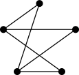
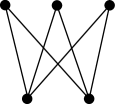
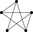
$\cong$       $\cong$  

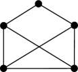
Figure 1: Non-QE graphs: G5-10 (left) and G5-17 (right)

3 Complete Multipartite Graphs

3.1 Definition and Basic Properties

For $k\geq 2$ let $V_{1},V_{2},\dots V_{k}$ be mutually disjoint non-empty finite sets. Setting

$$V=\bigcup_{i=1}^{k}V_{i},\qquad E=\bigcup_{i\neq j}\{\{x,y\}\,;\,x\in V_{i},\,y\in V_{j}\},$$

we obtain a graph $G=(V,E)$, which is called a complete $k$-partite graph with parts $V_{1},V_{2},\dots,V_{k}$ and is denoted by $KM(V_{1},V_{2},\dots,V_{k})$. A complete multipartite graph is a complete $k$-partite graph for some $k\geq 2$.

For $k\geq 2$ a complete $k$-partite graph is determined (up to graph isomorphisms) by the sequence $m_{1},m_{2},\dots,m_{k}$ defined by $m_{i}=|V_{i}|$ and is denoted by

$$K_{m_{1},m_{2},\dots,m_{k}}=KM(V_{1},V_{2},\dots,V_{k}).$$ (3.1)

Without loss of generality we may assume that $m_{1}\geq m_{2}\geq\dotsb\geq m_{k}\geq 1$. For simplicity we write $K_{1(k)}$ for $K_{1,1,\dots,1}$ (“$1$” appears $k$ times). Obviously,

$$K_{1(k)}=K_{1,1,\dots,1}=K_{k}$$

which is nothing else but the complete graph on $k$ vertices. Overusing our notation for the case of $k=1$ we understand that $KM(V_{1})$ is the empty graph on $V_{1}$, that is the complement to the complete graph $K_{m_{1}}$ so that

$$KM(V_{1})=\bar{K}_{m_{1}}.$$ (3.2)

We note that (3.1) is not valid for $k=1$.

For later use we list some basic properties of complete multipartite graphs, of which verification is straightforward and is omitted.

Lemma 3.1.

Let $k\geq 2$ and $m_{1}\geq m_{2}\geq\dotsb\geq m_{k}\geq 1$. Then $\mathrm{diam}(K_{m_{1},m_{2},\dots,m_{k}})=2$ unless $m_{1}=m_{2}=\dots=m_{k}=1$.

Lemma 3.2.

Let $k\geq 2$ and let $V_{1},V_{2},\dots,V_{k}$ be mutually disjoint non-empty finite sets. Consider an arbitrary partition:

$$\{V_{1},V_{2},\dots V_{k}\}=\{U_{1},\dots,U_{p}\}\cup\{U_{1}^{\prime},\dots,U_{q}^{\prime}\},$$

where $p\geq 1$, $q\geq 1$ and $p+q=k$. Then we have

$$KM(V_{1},V_{2},\dots V_{k})=KM(U_{1},U_{2},\dots U_{p})+KM(U_{1}^{\prime},U_{2}^{\prime},\dots U_{q}^{\prime}),$$

where the right-hand side is the graph join.

For example, we have

$$K_{m_{1},m_{2}} =\bar{K}_{m_{1}}+\bar{K}_{m_{2}},$$

$$K_{m_{1},m_{2},m_{3}} =\bar{K}_{m_{2}}+K_{m_{1},m_{3}},$$

$$K_{m_{1},m_{2},m_{3},m_{4}} =K_{m_{1},m_{3}}+K_{m_{2},m_{4}},\quad\text{etc.,}$$

where (3.2) is taken into account.

Next we study a subgraph of $KM(V_{1},V_{2},\dots V_{k})$. For $2\leq p\leq k$ let $U_{1},U_{2},\dots,U_{p}$ be $p$ parts chosen from $V_{1},V_{2},\dots V_{k}$. For each $1\leq i\leq p$ let $U_{i}^{\prime}\subset U_{i}$ be a non-empty subset. It is then easy to see that

$$KM(U_{1}^{\prime},U_{2}^{\prime},\dots U_{p}^{\prime})\hookrightarrow KM(V_{1},V_{2},\dots V_{k}).$$

This isometric embedding is stated as follows.

Lemma 3.3.

Let $m_{1}\geq m_{2}\geq\dotsb\geq m_{k}\geq 1$ and $n_{1}\geq n_{2}\geq\dotsb\geq n_{p}\geq 1$ be two sequences with $k\geq 2$ and $p\geq 2$. If there exist $1\leq i_{1}<i_{2}<\dots<i_{p}\leq k$ such that

$$n_{1}\leq m_{i_{1}},\quad n_{2}\leq m_{i_{2}},\quad\dots,\quad n_{p}\leq m_{i_{p}},$$

then we have

$$K_{n_{1},n_{2},\dots,n_{p}}\hookrightarrow K_{m_{1},m_{2},\dots,m_{k}}.$$

Obviously, any induced subgraph of $KM(V_{1},V_{2},\dots V_{k})$ is of the form $KM(U_{1}^{\prime},U_{2}^{\prime},\dots U_{p}^{\prime})$ as mentioned above. With the help of Lemma 2.2 we come to the following

Lemma 3.4.

Let $H$ be a subgraph of a complete $k$-partite graph $K_{m_{1},m_{2},\dots,m_{k}}$. If $H$ is a graph on two or more vertices and is isometrically embedded in $K_{m_{1},m_{2},\dots,m_{k}}$, then $H$ is a complete $p$-partite graph $K_{n_{1},n_{2},\dots,n_{p}}$ of the form as in Lemma 3.3.

3.2 Calculating QE Constants

Throughout this subsection, letting $k\geq 2$ and $m_{1}\geq m_{2}\geq\dots\geq m_{k}\geq 1$ be fixed, we set

$$G=K_{m_{1},m_{2},\dots,m_{k}}\,.$$

Our goal is to obtain an explicit formula for $\mathrm{QEC}(G)$. Since $1\leq\mathrm{diam}(G)\leq 2$ the following general result is useful.

Proposition 3.5.

[16, Proposition 2.1] Let $G$ be a graph with $1\leq\mathrm{diam}(G)\leq 2$. Let $A$ be the adjacency matrix of $G$ and set

$$\alpha_{\mathrm{min}}=\min\{\langle f,Af\rangle\,;\,\langle f,f\rangle=1,\,\,\,\langle{\bm{1}},f\rangle=0\}.$$ (3.3)

Then we have

$$\mathrm{QEC}(G)=-2-\alpha_{\mathrm{min}}.$$

Now let $A$ be the adjacency matrix of $G=K_{m_{1},m_{2},\dots,m_{k}}$. Then $A$ is written in a block matrix form:

$$A=\begin{bmatrix}0&J&J&\dots&J\\ J&0&J&\dots&J\\ \vdots&\vdots&\ddots&&\vdots\\ J&J&\dots&0&J\\ J&J&\dots&J&0\end{bmatrix}=J-\begin{bmatrix}J&0&0&\dots&0\\ 0&J&0&\dots&0\\ \vdots&\vdots&\ddots&&\vdots\\ 0&0&\dots&J&0\\ 0&0&\dots&0&J\end{bmatrix},$$ (3.4)

where $J$ is a matrix of which entries are all one and the size is understood in the context. For example, in the last block matrix in (3.4) $J$’s appear as diagonal entries. We understand naturally that their sizes are $m_{1}\times m_{1},\dots,m_{k}\times m_{k}$ from left top to right bottom.

We will find the conditional minimum $\alpha_{\mathrm{min}}$ in (3.3). According to the block matrix form of the adjacency matrix $A$ in (3.4), any $f\in C(V)\cong\mathbb{R}^{m_{1}+\dots+m_{k}}$ is written as

$$f=\begin{bmatrix}f_{1}\\ f_{2}\\ \vdots\\ f_{k}\end{bmatrix},\qquad f_{i}=\begin{bmatrix}f_{i1}\\ f_{i2}\\ \vdots\\ f_{im_{i}}\end{bmatrix}\in\mathbb{R}^{m_{i}},\qquad 1\leq i\leq k.$$

Then we have

$$\langle f,Af\rangle=\langle f,Jf\rangle-\sum_{i=1}^{k}\langle f_{i},Jf_{i}\rangle=\langle{\bm{1}},f\rangle^{2}-\sum_{i=1}^{k}\langle{\bm{1}},f_{i}\rangle^{2}.$$ (3.5)

Upon applying the method of Lagrange’s multiplier we set

$$\varphi(f,\alpha,\beta)=\langle f,Af\rangle-\alpha(\langle f,f\rangle-1)-\beta\langle{\bm{1}},f\rangle.$$

By general theory we know that the conditional minimum (3.3) is attained at a certain stationary point. Let $\mathcal{S}$ be the set of all stationary points $(f,\alpha,\beta)$, that is, the set of solutions to

$$\frac{\partial\varphi}{\partial f_{ij}}=\frac{\partial\varphi}{\partial\alpha}=\frac{\partial\varphi}{\partial\beta}=0,\qquad 1\leq i\leq k,\quad 1\leq j\leq m_{i}\,.$$ (3.6)

After simple calculus (3.6) becomes the following system of equations:

$$(J+\alpha)f_{i}=-\frac{\beta}{2}\,{\bm{1}},\qquad 1\leq i\leq k,$$ (3.7)

$$\langle f,f\rangle=\sum_{i=1}^{k}\langle f_{i},f_{i}\rangle=1,$$ (3.8)

$$\langle{\bm{1}},f\rangle=\sum_{i=1}^{k}\langle{\bm{1}},f_{i}\rangle=0.$$ (3.9)

For $1\leq s\leq m_{i}$ the $s$th entry of the left-hand side of (3.7) is given by

$$((J+\alpha)f_{i})_{s}=\sum_{t=1}^{m_{i}}((J)_{st}+\alpha\delta_{st})f_{it}=\langle{\bm{1}},f_{i}\rangle+\alpha f_{is}\,.$$

Thus (3.7) is equivalent to

$$\langle{\bm{1}},f_{i}\rangle+\alpha f_{is}=-\frac{\beta}{2}\,,\qquad 1\leq s\leq m_{i}\,,\quad 1\leq i\leq k.$$ (3.10)

As a result, $\mathcal{S}$ is the set of all solutions $(f=[f_{i}],\alpha,\beta)$ to the equations (3.10), (3.8) and (3.9). For convenience we denote by $\mathcal{S}_{A}$ the set of all $\alpha\in\mathbb{R}$ appearing in $\mathcal{S}$, that is, $(f,\alpha,\beta)\in\mathcal{S}$ for some $f$ and $\beta$.

Lemma 3.6.

For any $(f,\alpha,\beta)\in\mathcal{S}$ we have $\langle f,Af\rangle=\alpha$. Therefore,

$$\alpha_{\mathrm{min}}=\min\mathcal{S}_{A}\,.$$

Proof.

Let $(f=[f_{i}],\alpha,\beta)\in\mathcal{S}$. Noting that the equations (3.7)–(3.9) are fulfilled, we have

$$\langle f_{i}\,,\,Jf_{i}\rangle=\bigg{\langle}f_{i}\,,\,-\alpha f_{i}-\frac{\beta}{2}\,{\bm{1}}\bigg{\rangle}=-\alpha\langle f_{i}\,,f_{i}\rangle-\frac{\beta}{2}\,\langle{\bm{1}},f_{i}\rangle$$

and hence

$$\sum_{i=1}^{k}\langle f_{i},Jf_{i}\rangle=-\alpha\sum_{i=1}^{k}\langle f_{i},f_{i}\rangle-\frac{\beta}{2}\,\sum_{i=1}^{k}\langle{\bm{1}},f_{i}\rangle=-\alpha.$$

On the other hand, by (3.9) we have

$$\langle f,Jf\rangle=\langle{\bm{1}},f\rangle^{2}=0.$$

Consequently, we see from (3.5) that

$$\langle f,Af\rangle=\langle f,Jf\rangle-\sum_{i=1}^{k}\langle f_{i},Jf_{i}\rangle=0-(-\alpha)=\alpha,$$

as desired. The assertion in the second half is then apparent. ∎

In order to study $\mathcal{S}_{A}$ we come back to the equations (3.7)–(3.9), where (3.7) is equivalent to (3.10).

Lemma 3.7.

If $(\xi_{1},\dots,\xi_{k},\alpha,\beta)\in\mathbb{R}^{k}\times\mathbb{R}\times\mathbb{R}$ satisfies

$$(m_{i}+\alpha)\xi_{i} =-\frac{\beta}{2}\,,\qquad 1\leq i\leq k,$$ (3.11)

$$\sum_{i=1}^{k}m_{i}\xi_{i}^{2} =1,$$ (3.12)

$$\sum_{i=1}^{k}m_{i}\xi_{i} =0,$$ (3.13)

then, setting $f_{i}=\xi_{i}{\bm{1}}$, we have $(f=[f_{i}],\alpha,\beta)\in\mathcal{S}$. Conversely, for any $(f=[f_{i}],\alpha,\beta)\in\mathcal{S}$ with $\alpha\neq 0$ there exist $\xi_{1},\dots,\xi_{k}\in\mathbb{R}$ such that $f_{i}=\xi_{i}{\bm{1}}$ and (3.11)–(3.13) are satisfied.

Proof.

It is straightforward to show that $(f=[f_{i}],\alpha,\beta)$ with $f_{i}=\xi_{i}{\bm{1}}$ satisfies (3.10), (3.8) and (3.9) under conditions (3.11)–(3.13). We prove the converse. Suppose that $\alpha\neq 0$ and $(f=[f_{i}],\alpha,\beta)$ is a solution to (3.10), (3.8) and (3.9). In view of $\alpha\neq 0$ we see from (3.10) that $f_{is}$ is constant independently of $1\leq s\leq m_{i}$. In other words, $f_{i}$ is a constant multiple of ${\bm{1}}$, say $f_{i}=\xi_{i}{\bm{1}}$ with $\xi_{i}\in\mathbb{R}$. Then equations (3.10), (3.8) and (3.9) are reduced to the equations (3.11), (3.12) and (3.13), respectively. ∎

Lemma 3.8.

If $\alpha\in\mathcal{S}_{A}$ and $\alpha\not\in\{0,-m_{1},-m_{2},\dots,-m_{k}\}$, then $\alpha$ satisfies

$$\sum_{i=1}^{k}\frac{m_{i}}{\alpha+m_{i}}=0.$$ (3.14)

Conversely, if $\alpha\in\mathbb{R}$ satisfies (3.14), then $\alpha\in\mathcal{S}_{A}$.

Proof.

Let $\alpha\in\mathcal{S}_{A}$ with $\alpha\not\in\{0,-m_{1},-m_{2},\dots,-m_{k}\}$. Then $(f,\alpha,\beta)\in\mathcal{S}$ for some $f$ and $\beta$ so that the equations (3.10), (3.8) and (3.9) are satisfied. By Lemma 3.7 there exist $\xi_{1},\dots,\xi_{k}\in\mathbb{R}$ such that $f_{i}=\xi_{i}{\bm{1}}$ such that $(f=[f_{i}],\alpha,\beta)$ fulfills (3.11)–(3.13). From (3.11) we have

$$\xi_{i}=-\frac{\beta}{2}\,\frac{1}{\alpha+m_{i}}\,,\qquad 1\leq i\leq k.$$ (3.15)

Then (3.12) and (3.13) become

$$\frac{\beta^{2}}{4}\sum_{i=1}^{k}\frac{m_{i}}{(\alpha+m_{i})^{2}} =1,$$ (3.16)

$$-\frac{\beta}{2}\sum_{i=1}^{k}\frac{m_{i}}{\alpha+m_{i}} =0,$$ (3.17)

respectively. We see from (3.16) that $\beta\neq 0$ and then from (3.17) we obtain (3.14).

For the converse assertion let $\alpha$ be a solution to (3.14). Noting that $\alpha\not\in\{-m_{1},-m_{2},\dots,-m_{k}\}$, we define $\xi_{i}$ by (3.15) and set $f_{i}=\xi_{i}{\bm{1}}$. Choosing $\beta$ satisfying (3.16), we see that $(f=[f_{i}],\alpha,\beta)\in\mathcal{S}$ and hence $\alpha\in\mathcal{S}_{A}$. ∎

Lemma 3.9.

If $m_{1}=m_{2}$, then $-m_{1}\in\mathcal{S}_{A}$.

Proof.

It is straightforward to see that equations (3.11)–(3.13) are fulfilled by

$$\xi_{1}=\frac{1}{\sqrt{2m_{1}}}\,,\qquad\xi_{2}=-\frac{1}{\sqrt{2m_{1}}}\,,\qquad\xi_{i}=0,\quad 3\leq i\leq k,$$

$$\alpha=-m_{1},\qquad\beta=0.$$

It then follows from Lemma 3.7 that $(f=[f_{i}],\alpha,\beta)$ with $f_{i}=\xi_{i}{\bm{1}}$, $\alpha=-m_{1}$ and $\beta=0$ belongs to $\mathcal{S}$. Hence $-m_{1}\in\mathcal{S}_{A}$. ∎

Lemma 3.10.

If $m_{1}>m_{2}$, then $-m_{1}\not\in\mathcal{S}_{A}$.

Proof.

Suppose that $-m_{1}\in\mathcal{S}_{A}$. Then $(f,-m_{1},\beta)\in\mathcal{S}$ for some $f$ and $\beta$. Since $\alpha=-m_{1}\neq 0$, by Lemma 3.7 there exist $\xi_{1},\dots,\xi_{k}\in\mathbb{R}$ satisfying (3.11)–(3.13). Note that (3.11) becomes

$$(m_{i}-m_{1})\xi_{i}=-\frac{\beta}{2}\,,\qquad 1\leq i\leq k.$$ (3.18)

Putting $i=1$, we obtain $\beta=0$ and (3.18) becomes

$$(m_{i}-m_{1})\xi_{i}=0,\qquad 1\leq i\leq k.$$ (3.19)

Since $m_{1}>m_{2}\geq m_{3}\geq\dotsb\geq m_{k}\geq 1$ by assumption, we see from (3.19) that $\xi_{i}=0$ for $2\leq i\leq k$. It then follows from (3.13) that $\xi_{1}=0$ too. Thus we obtain $\xi_{i}=0$ for all $1\leq i\leq k$, which contradicts (3.12). Consequently, $-m_{1}\not\in\mathcal{S}_{A}$. ∎

We are now in a position to sum up the above argument.

Proposition 3.11.

Let $k\geq 2$ and $m_{1}\geq m_{2}\geq\dotsb\geq m_{k}\geq 1$. Let $A$ be the adjacency matrix of the complete $k$-partite graph $K_{m_{1},m_{2},\dots,m_{k}}$ and set

$$\alpha_{\mathrm{min}}=\min\{\langle f,Af\rangle\,;\,\langle f,f\rangle=1,\,\,\,\langle{\bm{1}},f\rangle=0\}.$$

1. If $m_{1}=m_{2}$, then $\alpha_{\mathrm{min}}=-m_{1}$.

2. If $m_{1}>m_{2}$, then $\alpha_{\mathrm{min}}=\alpha^{*}$, where $\alpha^{*}$ is the minimal solution to

   $$\sum_{i=1}^{k}\frac{m_{i}}{\alpha+m_{i}}=0.$$ (3.20)

   Moreover, $-m_{1}<\alpha^{*}<-m_{2}$.

Proof.

We set

$$\psi(\alpha)=\sum_{i=1}^{k}\frac{m_{i}}{\alpha+m_{i}}\,.$$

It follows from Lemma 3.8 that

$$\mathcal{S}_{A}\subset\{0,-m_{1},\dots,-m_{k}\}\cup\{\alpha\in\mathbb{R}\,;\,\psi(\alpha)=0\},$$ (3.21)

where $\{\alpha\in\mathbb{R}\,;\,\psi(\alpha)=0\}=\emptyset$ may occur. Since $\psi(\alpha)<0$ for all $\alpha<-m_{1}$, we have $\{\alpha\in\mathbb{R}\,;\,\psi(\alpha)=0\}\subset(-m_{1},+\infty)$. Therefore, the minimum of the right-hand side of (3.21) is $-m_{1}$.

(1) By Lemma 3.9 we know that $-m_{1}\in\mathcal{S}_{A}$. We then see from (3.21) that $\min\mathcal{S}_{A}=-m_{1}$ so that $\alpha_{\mathrm{min}}=-m_{1}$.

(2) We first note from $m_{1}>m_{2}$ that $\psi(\alpha)=0$ has a solution. Hence the minimal solution $\alpha^{*}$ certainly exists and, as is easily verified by simple calculus, we have $-m_{1}<\alpha^{*}<-m_{2}$. Moreover, $\alpha^{*}\in\mathcal{S}_{A}$ by Lemma 3.8. On the other hand, $-m_{1}\not\in\mathcal{S}_{A}$ by Lemma 3.10. Therefore, $\min\mathcal{S}_{A}=\alpha^{*}$ so that $\alpha_{\mathrm{min}}=\alpha^{*}$. ∎

We now come to the first main result.

Theorem 3.12 (Theorem 1.1).

Let $k\geq 2$ and $m_{1}\geq m_{2}\geq\dotsb\geq m_{k}\geq 1$.

1. If $m_{1}=m_{2}$, we have $\mathrm{QEC}(K_{m_{1},m_{2},\dots,m_{k}})=-2+m_{1}$.

2. If $m_{1}>m_{2}$, we have $\mathrm{QEC}(K_{m_{1},m_{2},\dots,m_{k}})=-2-\alpha^{*}$, where $\alpha^{*}$ is the minimal solution to (3.20). Moreover, $-m_{1}<\alpha^{*}<-m_{2}$.

Proof.

Straightforward from Propositions 3.5 and 3.11. ∎

3.3 Some Special Cases

We apply Theorem 3.12 to some special cases.

Example 3.13 (See Example 2.7).

The QE constant of a bipartite graph $K_{m,n}$ is obtained by simple algebra. If $m=n\geq 1$, we have

$$\mathrm{QEC}(K_{m,m})=-2+m.$$ (3.22)

If $m>n$, we have

$$\mathrm{QEC}(K_{m,n})=\frac{2(m-1)(n-1)-2}{m+n}\,.$$ (3.23)

The former formula (3.22) is reproduced by setting $m=n$ in the latter (3.23). Moreover, since the right-hand side of (3.23) is symmetric in $m$ and $n$, we see that (3.23) is valid for any $m\geq 1$ and $n\geq 1$.

Example 3.14.

The QE constant of a tripartite graph $K_{l,m,n}$ is obtained by simple algebra. If $l=m\geq n\geq 1$, we have

$$\mathrm{QEC}(K_{l,l,n})=-2+l.$$ (3.24)

Consider the case of $l>m\geq n\geq 1$. The equation (3.20) becomes

$$\frac{l}{\alpha+l}+\frac{m}{\alpha+m}+\frac{n}{\alpha+n}=0$$

and the minimal solution is given by

$$\alpha^{*}=-\frac{lm+mn+nl+\sqrt{(lm+mn+nl)^{2}-3lmn(l+m+n)}}{l+m+n}\,.$$

Then we have

$$\mathrm{QEC}(K_{l,m,n})=-2+\frac{lm+mn+nl+\sqrt{(lm+mn+nl)^{2}-3lmn(l+m+n)}}{l+m+n}\,.$$ (3.25)

By simple algebra we see that (3.24) is reproduced from (3.25) by setting $l=m$. Moreover, since the right-hand side of (3.25) is symmetric in $l,m$ and $n$, we conclude that the formula (3.25) is valid for any $l\geq 1$, $m\geq 1$ and $n\geq 1$.

Example 3.15 (see Example 2.8).

Let $m\geq 1$ and $n\geq 1$. The $(n+1)$-partite graph $K_{m,1(n)}$ coincides with the graph join $\bar{K}_{m}+K_{n}$, which is known as a complete split graph. The QE constant is obtained by simple algebra. If $m=1$, we have

$$\mathrm{QEC}(K_{1,1(n)})=-2+1=-1.$$ (3.26)

In fact, $K_{1,1(n)}=K_{n+1}$ is the complete graph and the result is mentioned also in Example 2.4. Assume that $m>1$. The minimal solution to

$$\frac{m}{\alpha+m}+\frac{n}{\alpha+1}=0$$

is given by $\alpha^{*}=-m(n+1)/(m+n)$ and we then come to

$$\mathrm{QEC}(K_{m,1(n)})=-2-\alpha^{*}=-2+\frac{m(n+1)}{m+n}=\frac{(m-2)(n-1)-2}{m+n}\,.$$ (3.27)

Note that (3.26) is reproduced from (3.27) by setting $m=1$. Hence the formula (3.27) is valid for any $m\geq 1$ and $n\geq 1$.

Example 3.16.

For $n\geq 2$ the complete multipartite graph $K_{2(n)}$ is called a cocktail party graph or a hyperoctahedral graph. A straightforward application of Theorem 3.12 yields

$$\mathrm{QEC}(K_{2(n)})=0.$$

Note that $K_{2(n)}$ is obtained by deleting $n$ disjoint edges from the complete graph $K_{2n}$. It is known [18] that the QE constant of a graph obtained by deleting two or more disjoint edges from a complete graph is zero.

4 Primary Non-QE Graphs

4.1 Complete Multipartite Graphs of Non-QE Class

With the help of Theorem 3.12 (Theorem 1.1 in Introduction) all complete multipartite graphs of non-QE class are determined.

Let $k\geq 2$ and $m_{1}\geq m_{2}\geq\dotsb\geq m_{k}\geq 1$. If $m_{1}\geq 3$ and $m_{2}\geq 2$, then $K_{m_{1},m_{2},\dots,m_{k}}$ is of non-QE class because $K_{3,2}\hookrightarrow K_{m_{1},m_{2},\dots,m_{k}}$ and $K_{3,2}$ is of non-QE class. We will examine the rest cases.

(Case 1) $m_{1}\geq 3$ and $m_{2}=1$. In that case we have $m_{1}>m_{2}=\dots=m_{k}=1$ so that $K_{m_{1},m_{2},\dots,m_{k}}=K_{m_{1},1(k-1)}$ becomes a complete split graph. Using the formula (3.27) in Example 3.15, we obtain

$$\mathrm{QEC}(K_{m_{1},1(k-1)})=\frac{(m_{1}-2)(k-2)-2}{m_{1}+k-1}\,.$$

Hence $\mathrm{QEC}(K_{m_{1},1(k-1)})>0$ if and only if one of the following three conditions are fulfilled: (i) $k\geq 3$ and $m_{1}\geq 5$; (ii) $k\geq 4$ and $m_{1}\geq 4$; (iii) $k\geq 5$ and $m_{1}\geq 3$.

(Case 2) $m_{1}=2$. If $m_{1}=m_{2}$, we see from Theorem 3.12 that

$$\mathrm{QEC}(K_{2,2,m_{3},\dots,m_{k}})=-2+m_{1}=0.$$

If $m_{1}>m_{2}$, we have $m_{2}=\dots=m_{k}=1$. Applying the formula (3.27), we have

$$\mathrm{QEC}(K_{2,1(k-1)})=-\frac{2}{k+1}<0.$$

(Case 3) $m_{1}=1$. In that case we have $m_{2}=\dots=m_{k}=1$ so that $K_{1(k)}=K_{k}$ becomes a complete graph. We know that $\mathrm{QEC}(K_{1(k)})=-1$.

Thus, there are no non-QE graphs in Cases 2 and 3. Summing up the above argument, we claim the following

Theorem 4.1 (Theorem 1.2).

Let $m_{1}\geq m_{2}\geq\dotsb\geq m_{k}\geq 1$ with $k\geq 2$. Then the complete $k$-partite graph $K_{m_{1},m_{2},\dots,m_{k}}$ is of non-QE class if and only if one of the following conditions is satisfied:

1. $m_{1}\geq 3$ and $m_{2}\geq 2$,

2. $k\geq 3$, $m_{1}\geq 5$ and $m_{2}=\dots=m_{k}=1$,

3. $k\geq 4$, $m_{1}=4$ and $m_{2}=\dots=m_{k}=1$,

4. $k\geq 5$, $m_{1}=3$ and $m_{2}=\dots=m_{k}=1$.

The four families of complete multipartite graphs in Theorem 4.1 are mutually exclusive. With the help of Lemma 3.4, from each family we find a primary non-QE graph. The result is stated in the following

Theorem 4.2 (Theorem 1.3).

Among the complete multipartite graphs there are four primary non-QE graphs, which are listed with their QE constants as follows:

$$\mathrm{QEC}(K_{3,2})=2/5,$$

$$\mathrm{QEC}(K_{5,1,1})=1/7,$$

$$\mathrm{QEC}(K_{4,1,1,1})=2/7,$$

$$\mathrm{QEC}(K_{3,1,1,1,1})=1/7.$$

Moreover, any complete multipartite graph of non-QE class contains at least one of the above four primary non-QE graphs as an isometrically embedded subgraph.

4.2 Exploring Primary Non-QE graphs

In Theorem 4.2 we find three primary non-QE graphs on seven vertices. Note also that they are all complete split graphs:

$$K_{5,1,1} =\bar{K}_{5}+K_{2}=\text{G7-351},$$

$$K_{4,1,1,1} =\bar{K}_{4}+K_{3}=\text{G7-774},$$

$$K_{3,1,1,1,1} =\bar{K}_{3}+K_{4}=\text{G7-845},$$

where G$n$-$x$ stands for the graph on $n$ vertices with number $x$ in the list of small graphs due to McKay [13].

On the other hand, as is mentioned in Example 2.9, there are exactly two primary non-QE graphs on five vertices. Moreover, it is proved [17] that there are exactly three primary non-QE graphs on six vertices. They are the graphs G6-30, G6-60 and G6-84, see Figure 2. For the readers’ convenience, we record their QE constants:

$$\mathrm{QEC}(\text{G6-30}) =\frac{-4+\sqrt{19}}{3}\approx 0.1196,$$

$$\mathrm{QEC}(\text{G6-60}) =\lambda_{60}^{*}\approx 0.2034,$$

$$\mathrm{QEC}(\text{G6-84}) =\lambda_{84}^{*}\approx 0.1313,$$

where $\lambda_{60}^{*}$ is the unique positive root of $5\lambda^{3}+26\lambda^{2}+24\lambda-6=0$, and $\lambda_{84}^{*}$ is the unique positive root of $3\lambda^{4}+14\lambda^{3}+18\lambda^{2}+5\lambda-1=0$.

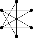
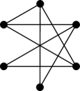
Figure 2: Primary non-QE graphs: G6-30, G6-60 and G6-84 (from left to right)

In this line an interesting question is to systematically construct primary non-QE graphs and to study the distribution of their QE constants.

Acknowledgements: This work is supported by JSPS Grant-in-Aid for Scientific Research No. 19H01789. The author is grateful to the referees for their useful comments which improved the paper.

References

• [1] A. Y. Alfakih: “Euclidean Distance Matrices and Their Applications in Rigidity Theory,” Springer, Cham, 2018.
• [2] M. Aouchiche and P. Hansen: Distance spectra of graphs: a survey, Linear Algebra Appl. 458 (2014), 301–386.
• [3] R. Balaji and R. B. Bapat: On Euclidean distance matrices, Linear Algebra Appl. 424 (2007), 108–117.
• [4] E. T. Baskoro and N. Obata: Determining finite connected graphs along the quadratic embedding constants of paths, Electron. J. Graph Theory Appl. 9 (2021), 539–560.
• [5] W. Irawan and K. A. Sugeng: Quadratic embedding constants of hairy cycle graphs, Journal of Physics: Conference Series 1722 (2021) 012046.
• [6] G. Jaklič and J. Modic: On Euclidean distance matrices of graphs, Electron. J. Linear Algebra 26 (2013), 574–589.
• [7] G. Jaklič and J. Modic: Euclidean graph distance matrices of generalizations of the star graph, Appl. Math. Comput. 230 (2014), 650–663.
• [8] Y.-L. Jin and X.-D. Zhang: Complete multipartite graphs are determined by their distance spectra, Linear Algebra Appl. 448 (2014), 285–291.
• [9] H. Lin, Y. Hong, J. Wang, J. Shub: On the distance spectrum of graphs, Linear Algebra Appl. 439 (2013), 1662–1669.
• [10] L. Liberti, G. Lavor, N. Maculan and A. Mucherino: Euclidean distance geometry and applications, SIAM Rev. 56 (2014), 3–69.
• [11] R. Liu, J. Xue and L. Guo: On the second largest distance eigenvalue of a graph, arXiv:1504.04225v1, 2015.
• [12] Z. Z. Lou, N. Obata and Q. X. Huang: Quadratic embedding constants of graph joins, Graphs and Combinatorics 38 (2022), 161.
• [13] B. McKay: All small connected graphs, online (2022.06.10)
http://www.cadaeic.net/graphpics.htm
• [14] W. Młotkowski: Quadratic embedding constants of path graphs, Linear Algebra Appl. 644 (2022), 95–107.
• [15] W. Młotkowski and N. Obata: On quadratic embedding constants of star product graphs, Hokkaido Math. J. 49 (2020), 129–163.
• [16] N. Obata: Quadratic embedding constants of wheel graphs, Interdiscip. Inform. Sci. 23 (2017), 171–174.
• [17] N. Obata: Primary non-QE graphs on six vertices, Interdiscip. Inform. Sci. 29 (2023), 141–156.
• [18] N. Obata and A. Y. Zakiyyah: Distance matrices and quadratic embedding of graphs, Electronic J. Graph Theory Appl. 6 (2018), 37–60.
• [19] M. Purwaningsih and K. A. Sugeng: Quadratic embedding constants of squid graph and kite graph, J. Phys.: Conf. Ser. 1722 (2021) 012047.
• [20] I. J. Schoenberg: Remarks to Maurice Fréchet’s article “Sur la définition axiomatique d’une classe d’espace distanciś vectoriellement applicable sur l’espace de Hilbert”, Ann. of Math. 36 (1935), 724–732.
• [21] I. J. Schoenberg: Metric spaces and positive definite functions, Trans. Amer. Math. Soc. 44 (1938), 522–536.