Single Pulse Variability in Gamma-ray Pulsars

Abstract

The Fermi Large Area Telescope receives $\ll$1 photon per rotation from any $\gamma$-ray pulsar. However, out of the billions of monitored rotations of the bright pulsars Vela (PSR J0835$-$4510) and Geminga (PSR J0633$+$1746), a few thousand have $\geq$2 pulsed photons. These rare pairs encode information about the variability of pulse amplitude and shape. We have cataloged such pairs and find the observed number to be in good agreement with simple Poisson statistics, limiting any amplitude variations to $<$19% (Vela) and $<$22% (Geminga) at 2$\sigma$ confidence. Using an array of basis functions to model pulse shape variability, the observed pulse phase distribution of the pairs limits the scale of pulse shape variations of Vela to $<$13% while for Geminga we find a hint of $\sim$20% single-pulse shape variability most associated with the pulse peaks. If variations last longer than a single rotation, more pairs can be collected, and we have calculated upper limits on amplitude and shape variations for assumed coherence times up to 100 rotations, finding limits of $\sim$1% (amplitude) and $\sim$3% (shape) for both pulsars. Because a large volume of the pulsar magnetosphere contributes to $\gamma$-ray pulse production, we conclude that the magnetospheres of these two energetic pulsars are stable over one rotation and very stable on longer time scales. All other $\gamma$-ray pulsars are too faint for similar analyses. These results provide useful constraints on rapidly-improving simulations of pulsar magnetospheres, which have revealed a variety of large-scale instabilities in the thin equatorial current sheets where the bulk of GeV $\gamma$-ray emission is thought to originate.

1 Introduction

Our understanding of pulsar magnetospheres is improving rapidly: sophisticated simulations are providing the first nearly self-consistent realizations of magnetospheres, and the Fermi Large Area Telescope (LAT) continues its groundbreaking discovery and characterization of the large population of $\gamma$-ray pulsars needed to test these models.

These new particle-in-cell (PIC) simulations rest on half a century of theoretical work. Soon after Hewish et al. (1968) discovered pulsars, Goldreich & Julian (1969) proposed a “force-free” (FF) model of the pulsar magnetosphere in which a co-rotating charge-separated plasma with density $\rho_{\mathrm{GJ}}\sim\Omega\cdot B$ screens the parallel electric field ($E_{\parallel}$), a picture which largely holds up today. However, FF magnetospheres by definition cannot accelerate particles, and the necessity of strong acceleration with concomitant $e^{+}$/$e^{-}$ pair formation in active pulsars was quickly recognized (Sturrock, 1971). Moreover, solving the coupled currents and electrodynamics even with the FF constraint proved intractable, and the best available analytic model was that of a magnetic dipole rotating in vacuo (Deutsch, 1955), also clearly far from reality.

These difficulties led to long threads of research which compartmentalized the problem. To characterize particle acceleration, theorists supposed that in an otherwise FF magnetosphere, small regions might lack the $\rho=\rho_{\mathrm{GJ}}$ plasma needed to screen the electric field. Such vacuum “gaps” could accelerate particles to high energy and form the pairs needed to achieve the assumed force-free conditions elsewhere. The ideas included a gap operating above the magnetic polar cap (Ruderman & Sutherland, 1975), a “slot gap” arising around the polar cap rim (Arons, 1983), and an “outer gap” operating above the null charge surface ($\rho_{\mathrm{GJ}}=0$) near the light cylinder (Cheng et al., 1986).

$\gamma$ rays are ideal for testing these models, as they directly trace particle acceleration. Observations by COS-B and EGRET (e.g. Thompson et al., 1999) provided both pulse profiles and spectra for a half-dozen young pulsars. Even in small numbers, it was clear that the light curves differed substantially from radio pulses, arriving later in the neutron star rotation (by a phase lag commonly notated $\delta$) and demonstrating a now-canonical morphology of two cuspy peaks separated by $\Delta$$\sim$0.2–0.5 rotations. Comparison to data was achieved using a “geometric” method which propagated $\gamma$-ray emissitivities to an observer using the Deutsch field. Approximately offsetting effects from time delay and field sweepback produced caustic-like features (Romani & Yadigaroglu, 1995) more reminiscent of the data than the predictions of low-altitude models (Daugherty & Harding, 1996), lending some credence to an outer magnetospheric origin. However, the small pulsar numbers and incomplete magnetic field information could not support strong conclusions.

Thirty years after the proposal of the idea, Contopoulos et al. (1999) and Timokhin (2006) numerically solved the FF magnetohydrodynamic equations for an aligned ($\Omega\parallel B$) magnetosphere while later work (Spitkovsky, 2006; Kalapotharakos & Contopoulos, 2009) addressed the nonaligned cases. These breakthrough solutions finally provided an exact description of both fields and currents, revealing a key feature: current flows out of the polar cap into a broad volume of the magnetosphere, but much of it returns in a very thin layer in the equatorial plane, splitting at the “separatrix” near the light cylinder and returning to the rim of the polar cap along the boundary of the closed and open magnetic field zones. This equatorial current sheet (ECS) is a hallmark of FF magnetospheres, though less of the return current flows through the ECS for large magnetic inclinations. Its extremely high areal current density makes it a natural candidate for magnetic reconnection and accelerating fields, but assessing these processes cannot be done with FF MHD.

This development set the stage for an observational revolution: soon after its launch, the Fermi Large Area Telescope (LAT, Atwood et al., 2009) detected populations of radio-loud, radio-quiet (Abdo et al., 2009a), and millisecond pulsars (Abdo et al., 2009b), establishing all classes as efficient $\gamma$-ray emitters capable of converting $\sim$1–30% of their available spin-down power (Abdo et al., 2013) into GeV photons. Early analyses of the LAT data strongly supported the outer magnetosphere as the most likely site of substantial $\gamma$-ray production. First, the spectral signatures of bright pulsars lacked evidence for attenuation in the strong magnetic fields above polar caps (Abdo et al., 2009c). Second, the fraction of pulsars with radio-trailing, cuspy double-peaked light curves was too large for low-altitude emission models (e.g. Watters et al., 2009). However, the expanding pulsar population soon challenged the simple geometric prescriptions, and e.g. Pierbattista et al. (2015) found in general that radio-loud $\gamma$-ray pulsars cannot be consistently modeled with any combination of a “gap” accelerator and the vacuum magnetic field.

Bai & Spitkovsky (2010) reinforced this discrepancy, finding that replacing the Deutsch field with a FF magnetosphere yielded poor agreement with Fermi data when paired with existing gap models, largely due to the increased field sweepback. Instead, these authors invoked a “separatrix layer model” operating along the ECS, extending even further into the outer magnetosphere than the classic outer gap model. Relaxing the FF assumptions by introducing resistivity into the magnetosphere—thus emulating conversion of the fields and currents into high-energy particles—yielded even better agreement. Kalapotharakos et al. (2014) used a prescription which was FF inside the light cylinder and resistive outside, with the resulting tweaks to the magnetic field and emission geometry producing the first excellent agreement with the observed $\delta$-$\Delta$ properties of the LAT pulsar sample (Abdo et al., 2013). This and other work cemented the paradigm that $\gamma$-ray pulsars have nearly force-free magnetospheres and produce most of their $\gamma$ rays in the ECS near and beyond the light cylinder.

Recent PIC simulations have confirmed this picture with, for the first time, nearly self-consistent modeling. In PIC simulations, macroparticles representing collections of many charged particles are evolved iteratively with the electromagnetic fields tabulated at the cell boundaries. The particles produce the (non background) fields and are in turn accelerated by them. The dynamic range of the simulations is still many orders of magnitude below a true magnetosphere, so e.g. maximum particle Lorentz factors reach $\sim$1000. Thus the key process of pair production must still be put in manually. Timokhin & Arons (2013) demonstrated that a current density $J\equiv c\rho$ of $J/J_{\mathrm{GJ}}<0$ or $J/J_{\mathrm{GJ}}>1$ is indicative of intense particle acceleration and pair production, while for $0<J/J_{\mathrm{GJ}}<1$, current can be sustained by space-charge limited flow with no pair production. This provides a common prescription for PIC simulations: by requiring that $J/J_{\mathrm{GJ}}>1$, authors can assume pair production occurs locally and replace the primary particles with secondaries and $\gamma$ rays, thus providing both the copious plasma needed to screen the electric field and tracking the emission of $\gamma$ rays for comparison to observation.

With such prescribed pair injection, PIC simulations have been successful in reproducing the general structure of FF magnetospheres but offer more insight into the dynamics, in particular the response of the magnetosphere to the location and extent of pair production. E.g., Philippov et al. (2015a) found that the incorporation of General Relativistic effects near the neutron star surface suppresses $\rho_{\mathrm{GJ}}$ locally, facilitating the pair production needed to explain the presence of radio pulsations. However, Chen et al. (2020, and see also () for similar studies), simulating magnetospheres over a range of pair production rates, highlight the importance of pairs within the ECS to achieving a near-FF magnetosphere due to the difficulty in screening $E_{\parallel}$ there. If pairs produced elsewhere (Cerutti et al., 2015; Brambilla et al., 2018) are unable to enter the ECS, or the sheet itself is no longer able to support pair production, the magnetosphere may transition to a static, charge-separated electrosphere. In the intermediate regime, the magnetosphere fluctuates between these states, with $\gamma$-ray production and global currents fluctuating in step.

As PIC simulations have been refined, they have become more predictive for $\gamma$-ray data. Kalapotharakos et al. (2018) and Philippov & Spitkovsky (2018) built $\gamma$-ray light curves by tracking emitted photons and found their pattern on the sky in reasonable agreement with data. Philippov & Spitkovsky (2018) postulate that $\gamma$ rays are primarily produced by synchrotron emission from reconnection in the ECS (Uzdensky & Spitkovsky, 2014), near the LC in the case of aligned rotators and from beyond the LC for oblique rotators, which are also somewhat less efficient emitters. On the other hand, Kalapotharakos et al. (2017) and Kalapotharakos et al. (2019) have noted that $\gamma$-ray properties lie on a “fundamental plane” according to their $\gamma$-ray luminosity, spectral cutoff energy, magnetic field, and spindown luminosity $\dot{E}$. By connecting the cutoff energy to the maximum particle Lorentz factors, they argue that the scaling is more indicative of curvature radiation. The upcoming third Fermi pulsar catalog will provide data for many more pulsars and provide a touchstone to determine which of these mechanisms is operant. Thus, after more than 50 years of work, theory and data are poised to deliver a nearly-complete picture of the pulsar magnetosphere and how it emits $\gamma$ rays.

Yet while the overall static picture is becoming clear, the PIC simulations have opened the field of magnetosphere dynamics and their observability. Notably, kink instabilities in the ECS are a common feature in PIC simulation results—especially near the Y-point/separatrix where the return current converges (Chen & Beloborodov, 2014)—with the local tangent to the ECS varying by $\sim$0.1 rad or more, which could affect the beaming of emitted $\gamma$ rays. If the $\gamma$ rays are emitted via magnetic reconnection, Uzdensky & Spitkovsky (2014) argue that the maximum size of coherent regions should be $<$100$\times$ the width of the current sheet, only about 1 m! Thus many reconnecting “islands” contribute to the current sheet and this could suppress such coherent effects, whereas dynamic instabilities could affect curvature radiation emission more significantly. On the other hand, reconnecting regions could merge into larger ones, driving $\gamma$-ray variability (Philippov et al., 2019; Ceyhun Andaç et al., 2022). Further, Kirk & Giacinti (2017) invoke a bulk Lorentz factor of $\sim$10⁴ in the wind of the Crab pulsar, in which case reconnection cannot proceed due to time dilation. In any case, for weaker pulsars, transitions between FF magnetospheres and “dead” electrospheres are common (Kalapotharakos et al., 2018; Philippov & Spitkovsky, 2018) and transitions can happen on timescales of one neutron star rotation (Chen et al., 2020) and longer.

$\gamma$-ray pulses, tracing both of these processes, would provide an invaluable probe for dynamics of the equatorial current sheet and the global magnetosphere. Accordingly, this work presents the first systematic search for and characterization of single- and few-pulse $\gamma$-ray pulse variability. Despite the recent theoretical motivation, such studies have heretofore been lacking primarily due to observational constraints: even the sensitive LAT records on average only $\sim$0.003 photons from Vela, the brightest $\gamma$-ray, during each 89 ms rotation, so measuring pulse-to-pulse profile or amplitude is impossible.

However, the LAT has observed billions of rotations of Vela, and $\sim$$10^{-6}$ of the rotations have 2 or more recorded photons. These multi-photon events are a far cry from a pulse, yet they still carry information about the variability of the pulsed GeV emission on short (neutron star rotation) time scales. For instance, any deviations from a constant flux would inevitably increase the number of observed pairs over the simple Poisson prediction. Likewise, pulse shape variations can be probed by examining the joint distribution of pulse phase for photon pairs. If certain portions of the pulse profile are brighter during some rotations than in others, this will manifest as a correlation in phase. Most generally, we expect simultaneous amplitude and shape variations: e.g., in a two-peaked pulse profile, a reduction in the intensity of one of the peaks could entail a reduction in total intensity, or it could be accompanied by an offsetting increase in the brightness of the other peak.

Below, we carry out a search for single- and mulitple-pulse variations in the two brightest $\gamma$-ray pulsars, Vela and Geminga. §2 presents our data preparation and selection of “photon pairs”. In §3, we search for amplitude variations independently and (finding none), we use the resulting limits as guidelines for a pulse shape variation search (§4) in which the total flux doesn’t vary by more than the established limits. We extend the analysis to longer timescales (up to 100 rotations) in §5, improving the constraints. We discuss other $\gamma$-ray pulsars, which are too faint to be of use, in §6, and we conclude in §7, placing our results in context and discussing the scant prospects for additional $\gamma$-ray variability measurements.

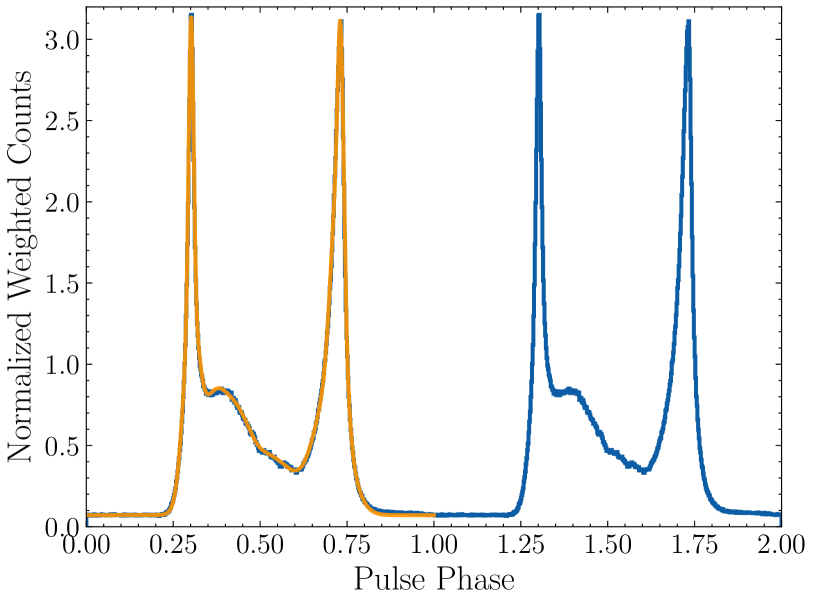
Figure 1: Two rotations of the Vela pulsar, showing a weighted histogram (500 bins per rotation, blue) of the full dataset and an analytic model for $f(\phi)$ overlaid (orange).

2 Data Preparation and Selection

We obtain “Pass 8” (Atwood et al., 2013) event reconstruction version P8R3 (Bruel et al., 2018) from the Fermi Science Support Center and process it using the Fermi Science Tools v2.0.0. We select about 12 years of data, between 2008 Aug 04 (MJD 54698) and an end date which depends on the range of validity of the pulsar timing solution (Table 1). We further restrict attention to events with reconstructed energy 0.1 GeV$<$E$<$10 GeV, measured zenith angle $<$100^∘, and a reconstructed incidence direction placing the photon within 3^∘ of the pulsar position. To enhance the sensitivity of the analyses (Bickel et al., 2008; Kerr, 2011, 2019), using the 4FGL DR2 sky model (Abdollahi et al., 2020; Ballet et al., 2020) and the P8R3_SOURCE_V3 instrument response function, we assign each photon a weight using gtsrcprob and restrict attention to events with $w>0.05$. This selection retains most of the signal while eliminating background photons that increase computational costs.

Name	Nickname	MJD End	Years
J0835$-$4510	Vela	59170	12.3
J0633$+$1746	Geminga	59249	12.5
J0534$+$2200	Crab	59000	11.9
J1709$-$4429	–	59312	12.6
J1057$-$5226	–	59249	12.5

Table 1: Some basic properties of the target sources and the data set. All data sets begin MJD 54698.

Type	Obs.	Chance	bona fide	Pred.
Vela
events	3,295,429	—	2,720,089.2	—
pairs	6,388	2,024.4	4,363.6	4,295.4
triples	12	6.6	5.4	4.7
Geminga
events	1,154,145	—	980,774.8	—
pairs	1,906	527.9	1,378.1	1,417.0
triples	5	2.4	2.6	1.5

Table 2: Observed total events and probability-weighted pairs and triples. The first column gives the total number of coincidences. The second tabulates the expected number of false positives (1 or more background events). The third column gives the prediction for the total number of true pairs (triples) based on the photon weights, while the fourth gives the prediction from the no-variability hypothesis, i.e. folding a constant rate through the instrument response function (see main text).

We obtain timing solutions for each pulsar using the maximum likelihood approach presented in Ajello (2022). Using PINT (Luo et al., 2021), we computed the absolute pulse phase for each event, and we define pairs as those photons with identical integer phase. This definition is somewhat arbitrary, but we have centered the pulse profile (Figure 1) within the phase window such that pairs associated with the same pulse are selected. (In §5, we adopt a simpler method of selecting photons whose total phase difference is simply less than some threshold, and we find no substantive difference.) Triples and higher-order coincidences follow the same definition.

Pursuing this method for Vela, we identified 6388 pairs, 12 triples, and no higher order coincidences. Because some photons come from the background, this total comprises three cases: two background photons, a single pulsed photon with a background photon, and two bona fide pulsed photons. The breakdown can be estimated from the photon weights, where $w_{1}$ and $w_{2}$ are the probability weights of the two photons in the observed pair: $\sum_{i}(1-w_{1i})(1-w_{2i})=188.9$ background pairs; $\sum_{i}(1-w_{1i})w_{2i}+w_{1i}(1-w_{2i})=1835.4$ with a single pulsed photon; and $\sum_{i}w_{1i}w_{2i}=4363.6$ bona fide pairs.

Similar arguments apply to the triples and we expect $\sum_{i}w_{1i}w_{2i}w_{3i}=5.4$ bona fide triples. These triples are too rare to be significantly constraining, so in the analysis below we focus on pairs. Table 2 summarizes these results for Vela and Geminga, including predictions accounting for the instrument exposure (see below).

3 Amplitude Variations

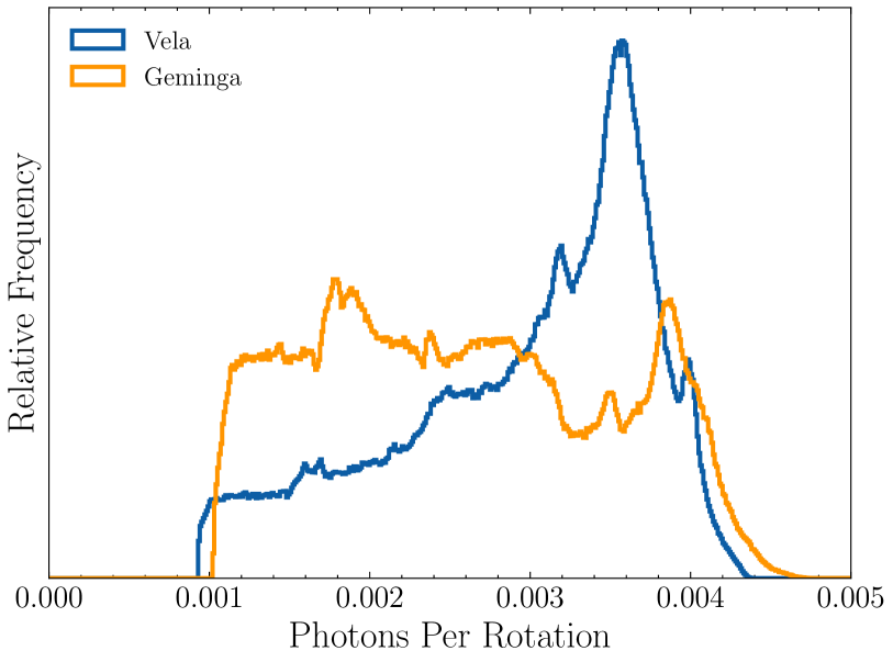
Figure 2: The distribution of the expected number of photons per rotation, averaged over a 30-s interval, for Vela and Geminga. The largest values correspond to the pulsar nearing the center of the field-of-view, and Vela accumulates more exposure under these favorable circumstances, enhancing the number of photon pairs expected relative to Geminga.

We test for amplitude variations against the null hypothesis—no variations—in which case the photon arrivals follow a Poisson distribution. To do this, we compute the expected number of photons for each rotation of the pulsar over the entire 12-year dataset by folding an average spectral energy distribution through the Fermi instrument response function.

In practice, we can ignore any intervals during which the pulsar is unobserved, as these have no constraining power. Moreover, the apparent angular motion of any source in the Fermi-LAT field-of-view over 30 s is $<$2^∘, allowing the exposure to be computed at this cadence with $<$0.1% error. So as to simplify the calculation, we determine the instantaneous photon rate over these 30 s intervals and assume it is the same for each pulsar rotation. As a further simplification, we ignore the spin evolution of the pulsar and simply use the mean spin rates of $\bar{\nu}=11.187519$ Hz for Vela and $\bar{\nu}=4.217539$ Hz for Geminga. With this prescription, the expected number of source photons per rotation is given by

$$\lambda_{30}=\frac{1}{\bar{\nu}}\int N(E)\epsilon(E,\cos(\theta_{30}))\,dE,$$ (1)

with $N(E)$ the photon spectral density (ph cm^-2 s^-1) for the pulsar and $\epsilon$ the effective area (cm²) for the given energy $E$ at an incidence angle $\theta_{30}$ taken to be constant over the 30 s interval. We evaluate $\lambda_{30}$ using the methods developed by Kerr (2019), particularly the package godot. In brief, this evaluation uses the tabulated spacecraft pointing history (“FT2 file”), with 30-s resolution, to determine $\cos\theta_{30}$ and hence the appropriate value of the tabulated effective area. Gaps in data taking are accounted for with the tabulated “Good Time Intervals” (GTI). The method also assumes a universal energy weighting $\propto$$E^{-2}$, which roughly describes the overall distribution of LAT photon energies. To further tune this approach for pulsars, which have spectral cutoffs at a few GeV, we perform the exposure calculation using 8 logarithmic bins spanning 100 MeV to 10 GeV. In each band, we then estimate the constant of proportionality to enforce $\sum_{i}\lambda_{30}^{i}=\sum_{i}w_{i}/30\mathrm{s}$. This accounts for any “local” differences in the distribution of photons from $\propto$$E^{-2}$ as well as for the reduction in effective exposure at low energies because the point spread function (PSF) is broader than the 3^∘ region of interest. We further note that we tabulate events which convert in the “front” (evtype 1) and “back” (evtype 2) of the tracker separately. We exclude any intervals with $\cos(\theta_{30})<0.4$, when the source is near or outside the edge of the LAT field-of-view. We further discard the lowest 0.5% of intervals, which eliminates a tail of low-exposure instances. The resulting rates (per rotation) for the two pulsars are shown in Figure 2. It is interesting to note that despite similar median photon rates (0.0032 and 0.0025 per rotation), Vela has three times as many photon pairs. As Figure 2 shows, Vela accumulates much more “high rate” exposure than Geminga, and this leads to more pair production. This intuitive explanation is borne out by the computations below and illustrates the importance of correcting for the instantaneous instrument exposure.

With the computed rates, we can predict the total number of pairs expected to be observed by using the Poisson distribution to evaluate the probability mass function of observing 0, 1, 2, or 3 photons during each rotation and summing these probabilities over all observed pulsar rotations. Using a simple model in which the pulsed flux is constant and only the instrumental exposure varies, for Vela this process yields $4,295.4\pm 65.5$ pairs (uncertainty assumes Poisson variance), in good agreement (1.0$\sigma$) with the observed, probability-weighted value of 4,363.6. Although triples are too rare to be constraining, the predicted number is 4.7, again in good agreement with the observation of 5.4. For Geminga, the prediction ($1,417.0\pm 37.6$) is higher than the observed value (1,378.1) and agrees at 1.0$\sigma$. All results are tabulated in Table 2.

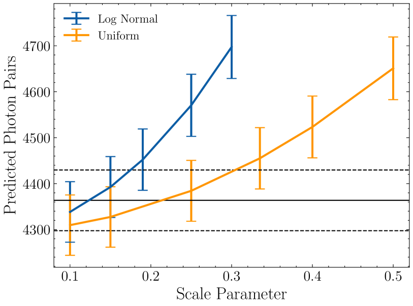
Figure 3: A comparison of the predicted count of bona fide photon pairs for two models along with the observed value (black line). The scale parameter corresponds to $\sigma$ in the case of the log normal model and width $W$ in the uniform model. The dashed lines indicate the 1$\sigma$ (Poisson) uncertainty range. See main text for details.

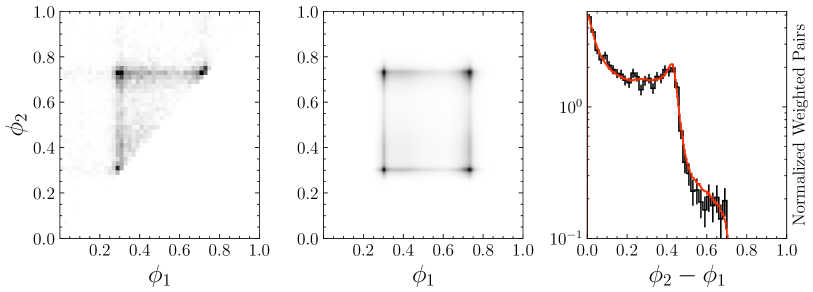
Figure 4: The joint distribution of phase for photon pairs, weighted by $w_{1}\times w_{2}$. The left panel shows the observed distribution sorted such that $\phi_{1}<\phi_{2}$. The center panel shows the expected null distrubtion $f(\phi_{1},\phi_{2})=f(\phi_{1})f(\phi_{2})$. The right panel gives the distribution of the sorted phase differences for the observed pairs, again weighted by $w_{1}\times w_{2}$, along with the expection from the null distribution, obtained by randomizing phases from the entire sample. Error bars are computed from the Poisson variance, which neglects the small correlations between bins.

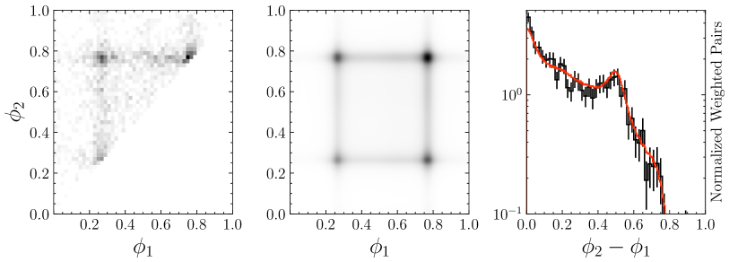
Figure 5: As Figure 4 for Geminga.

To gauge how large intrinsic flux variations could be without entering serious disagreement with the pair count, we consider two models of amplitude variations. First, we use a log normal distribution, with parameters $\mu$ and $\sigma$ for the underlying normal distribution. If we fix $\mu=-\sigma^{2}/2$, the distribution has unit mean, which preserves a constant photon rate but increases fluctuations between pulses. We then scale each value of $\lambda_{30}$ with a random draw from the distribution. (It is not necessary to draw a random variable for every pulsar rotation because the distribution is already sufficiently sampled by the millions of values of $\lambda_{30}$.) Second, we consider a uniform distribution with total width $2W$, which allows the relative values of $\lambda_{30}$ to vary by up to $1+W$, and we restrict $W\leq 1$ to avoid negative photon rates. These distributions differ strongly: in particular, the log normal distribution has heavy tails, allowing for very bright pulses, while the brightest pulses are capped in the uniform case.

The results of the study for Vela are shown in Figure 3. Increasing the scale parameters $\sigma$ and $W$ increases the number of predicted pairs until the predictions are no longer compatible with the observed value. If we adopt a 2$\sigma$ discrepancy for an upper limit, then scale parameters larger than $\sigma=0.21$ and $W=0.38$ are excluded. To put the models on equal footing we can compare their standard deviation ($\sigma_{w}=W/\sqrt{3}$ for the uniform case) and find $\sigma\approx\sigma_{w}$, and so in a relatively model independent fashion, we can exclude fluctuations whose typical strength exceeds 21%. A similar analysis for Geminga gives limits of $\sigma=0.16$ and $W=0.28$, limiting fluctuations to about 16%.

These results depend on the observed values, and so Geminga gives superior results despite having fewer pairs because the null pair prediction exceeds the observed value. We can instead simply consider the capability of the data to constrain variations without regard for the particular realization of it. With $\sim$4300 predicted (null hypothesis) pairs, the largest fractional increase in pair rate is $2\times 4300^{-\frac{1}{2}}$=3.0%, and for Geminga it is $2\times 1400^{-\frac{1}{2}}$=5.3%. These values correspond to $\sigma$ and $W$ parameters of 0.17 and 0.30 for Vela, and for Geminga 0.23 and 0.40, or relative variations of 17% and and 23% respectively.

4 Pulse Shape Variations

We now consider limits on the variation in pulse shape. Let the time-averaged pulse profile be $f(\phi)$. If normalized such that $\int_{0}^{1}f(\phi)=1$, this also is the probability density function (pdf) to observe a photon at the given phase. The pdf for the photon pairs is $f(\phi_{1},\phi_{2})$, normalized in the same way, and in the null hypothesis $\phi_{1}$ and $\phi_{2}$ are independent variables $f(\phi_{1},\phi_{2})=f(\phi_{1})f(\phi_{2})$. We can analyze any pairwise pulse shape variations using this distribution.

First, we characterize the distribution empirically. Figure 4 shows the observed joint probability distribution $f(\phi_{1},\phi_{2})$ for Vela as estimated with a weighted histogram, and the null expectation, namely $f(\phi_{1})f(\phi_{2})$. The data and this null model are visually in good agreement, though the small counts preclude assessment of goodness of fit. We have also examined the distribution of $\phi_{2}-\phi_{1}$, which also encodes information about correlations and is more sensitive to fluctuations with a constant scale $\delta\phi$. E.g., an enhancement of probability to observe a photon pair from either peak should produce an excess near the origin and a deficit elsewhere. This distribution, likewise, agrees well (within the uncertainty estimates) with the null hypothesis expectation, which we estimated by drawing random pairs from the much larger parent sample.

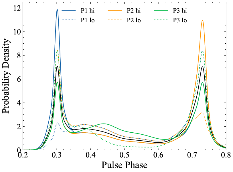
Figure 6: An example set of six basis functions for a model of single-pulse variations for Vela. They correspond to an addition (or loss) of 15% of the total flux from each of the three major components, P1, P2, and P3/the bridge. The time-averaged pulse profile is shown in black for reference. By construction, the mean of the six basis functions is equal to this pulse profile.

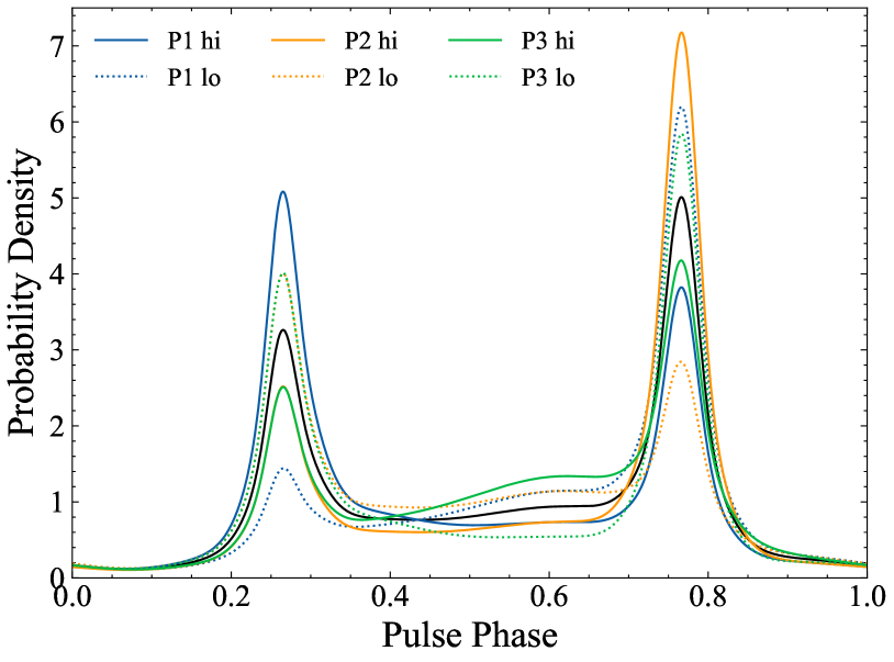
Figure 7: As Figure 6 for Geminga, but note different phase range.

We now seek to quantify the largest shape variations the data can accommodate. In doing so, we are guided by the results from §3 and the empirical analysis: the time-averaged distribution of photon pairs is very similar to $f(\phi)$, and if pulse shape variations are accompanied by intensity variations, they cannot be much larger than 20%. We also seek a physically motivated model: although the $\gamma$-ray emission contributing to a single spin phase can be accumulated from a large portion of the magnetosphere through caustic-like effects, the portions of the magnetosphere contributing to, e.g., P1, P2, and the bridge/P3 in Vela are distinct. Thus, considering changes localized to pulse profile features will target large-scale but distinct regions of the magnetosphere.

We thus adopt a family of $N_{b}$ basis functions, $b_{i}({\phi}$), which describe the variation in the pulse profile from rotation to rotation. Over many rotations, the individual pulse profiles must yield the long-term light curve, so by construction $\sum_{i}b_{i}({\phi})/N_{b}=f(\phi)$. For both Vela and Geminga, with well-defined two-peaked light curves and bridge emission, we choose $N_{b}=6$ corresponding to an increment and decrement of each of the three main features. The basis functions are defined via a strength parameter $\alpha$, with each basis function reducing to the null hypothesis: $b_{i}(\alpha,\phi)\rightarrow f(\phi)$ as $\alpha\rightarrow 0$. Figure 6 (7) illustrates the basis functions for Vela (Geminga) with $\alpha=0.15$ (15%) variations. Even this modest total variation results in changes of the relative peak amplitudes by about 2. And indeed, $\alpha$ cannot exceed $\sim$0.2 as this results in the removal of gross features of the light curve and a negative pdf. This is not a significant restriction since $\alpha=0.2$ already captures very large shape variations, and it ensures that the models tested in this analysis are consistent with the amplitude variation limits established above.

We proceed via maximum likelihood. On a given rotation, the photons are emitted according to one of the basis functions. Considering just a single pair of photons, the probability density function is then

$$(1-w_{1})(1-w_{2})+\sum_{i}\pi_{i}\big{[}w_{1}(1-w_{2})b_{i}(\alpha,\phi_{1})+$$ (2)

$$w_{2}(1-w_{1})b_{i}(\alpha,\phi_{2})+w_{1}w_{2}b_{i}(\alpha,\phi_{1})b_{i}(\alpha,\phi_{2})\big{]},$$

where the $\pi_{i}$ describe the probability of the $i$th basis function as being the correct one for the rotation in question. For convergence to the time-averaged profile, $<\pi_{i}>=1/N_{b}$. We have no a priori knowledge of $\pi_{i}$ for any given pulse, so we let it assume the time-averaged value $\pi=1/6$, allowing direct evaluation of the likelihood as a function of $\alpha$. The resulting log likelihood surface is shown in Figure 8. The likelihood peak for Vela is near $\alpha=0.08$, but the significance is consistent with $\alpha=0$. Consequently, we assume a uniform prior on $\alpha$ and estimate a 95% confidence upper limit of $\alpha<0.12$.

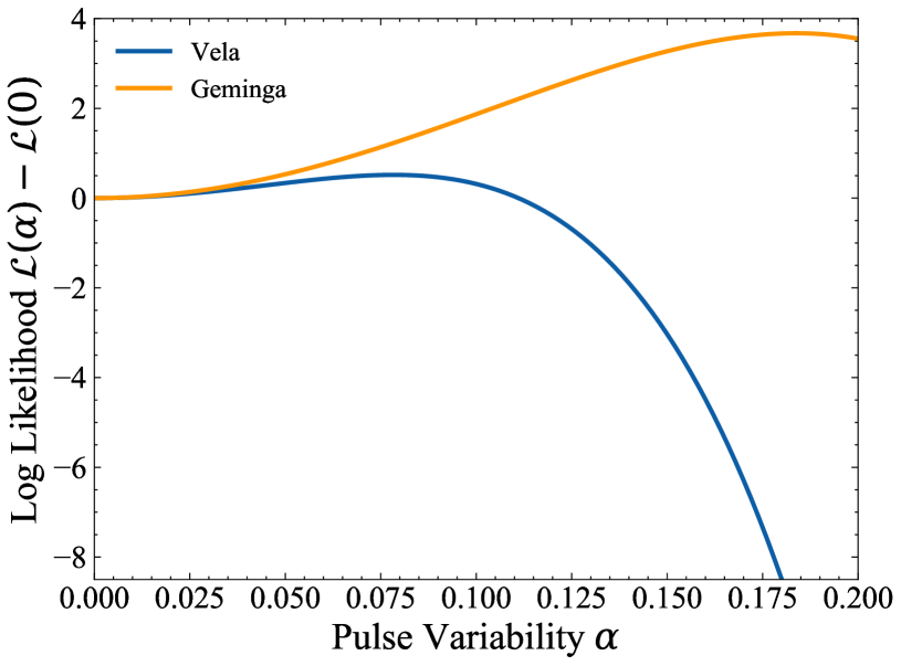
Figure 8: The log likelihood difference for Vela and Geminga for pulse shape variability characterized by a basis with strength $\alpha$ (see main text) relative to the null hypothesis.

Next, we consider the empirical distribution function for Geminga (Figure 5). As with Vela, it appears to largely follow the null hypothesis. The projected distribution in $\phi_{2}-\phi_{1}$ does show a small excess near the origin, indicating a possible small correlation for photons to arrive nearby in phase. Using the same basis-based technique (see Figure 7 for the basis functions for Geminga), we find the maximum likelihood value occuring around $\alpha=0.18$, with $\delta\log\mathcal{L}=3.67$, near the edge of the validity of our model. Because this model satisfies the conditions of Wilks’ Theorem, we can quickly estimate the significance of the alternative hypothesis as 99.3%. Thus there is modest evidence for pulse shape variability for Geminga, with an amplitude consistent with the largest allowed intensity variations. By skipping marginalization, we can determine the likelihood-maximizing basis function for each pair and thus obtain the distribution of preferred bases. We find bases which modify P1 and P2 are most prevalent, with P3 “hi” being least preferred. Thus, if the pulse shape variation is real, it is concentrated in the peaks, consistent with the empirical analysis above. However, we caution that this result strongly depends on our assumption of a particular basis.

5 Multi-rotation correlations

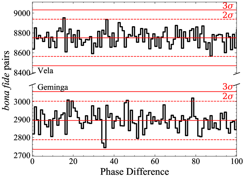
Figure 9: The observed bona fide photon pairs for Vela and Geminga, binned to integer phase differences. The expected number of pairs, as calculated by Monte Carlo siulations, and the 2- and 3-$\sigma$ uncertainties, are shown by horizontal lines. The data are in good agreement with an absence of amplitude fluctuations both in toto and for any particular phase separation.

We have also considered correlations on time scales greater than one neutron star rotation, which could be expected e.g. from magnetospheric state switching on longer time scales. We carried out a similar procedure, identifying photons with the requisite phase separation and using their weights to calculate the probability that they both originate from the pulsar. Here, we apply a simpler criterion, selecting as “pairs” those photons whose phase separation lies below a given threshold, say $\delta\phi<\Phi$. A threshold of $\Phi=0.5$ approximately reproduces the single-rotation selection above, while $\Phi=1$ produces about twice as many pairs, because it has contributions from two pulses.

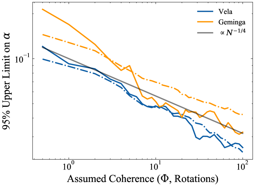
Figure 10: Limits on the strength of the variability parameter $\alpha$ (see main text) when including pairs collected over the indicated number of rotations. The solid lines give the results for the data, while dashed lines give the average of 10 Monte Carlo realizations in which any correlations in the real data have been broken. The scaling in both cases is in good agreement with the total number of pairs to the one-fourth power.

As before, we examine amplitude fluctuations by studying the total number of pairs up to an assumed coherence of $\Phi=100$ rotations, with results shown in Figure 9 for the two bright pulsars. Counting pairs based on exposure is more difficult in this case, because each rotation of the pulsar is no longer statistically independent. Thus, to calibrate the mean expectation, we use a simple Monte Carlo approach in which we permute the integer phase of each photon. This preserves the overall exposure pattern but breaks any short-term correlations. The resulting predictions, along with the corresponding Poisson uncertainties, are drawn in the figure. Because each of the observed pair counts lies within this band, we conclude there is no evidence for amplitude variations. By assuming longer coherence scale, the number of pairs increases substantially, and the limits on amplitude fluctuations tighten. The scaling simply depends on the total number of pairs, thus on $\Phi$, and we arrive at the limits on relative amplitude fluctuation for an assumed coherence time $\Phi$ in neutron star rotations: $<21\%(\Phi/0.5)^{-1/2}$ for Vela and $<16\%(\Phi/0.5)^{-1/2}$ for Geminga. For $\Phi=10$ this is 4.7% and 3.6%, and for $\Phi=100$, 1.5% and 1.1%.

Likewise, we can feed this larger population of pairs into the pulse shape analysis of §4. Here, because of the marginalization over the unknown basis for each pulse pair, the scaling with the number of pulses is less straightforward, and we have carried out the analysis directly on the data for the increasingly larger populations of pairs. The results, as a function of assumed coherence length $\Phi$, are shown in Figure 10. N.B. that the modest evidence for pulse shape variability in Geminga detected in §4 drops as soon as additional rotations are added and the limit quickly asymptotes to the same dependence as for Vela. For $\Phi=10$, the 95% limit on the shape variation parameter $\alpha$ is about 5% for both pulsars, and for $\Phi=100$ about 3%. The limits on the parameter seem to scale as the total observed pairs to the one-fourth power, rather than the one-half power as expected for Poisson uncertainties.

6 Other Bright Pulsars

Type	Obs.	Chance	bona fide	Pred.
J0534+2200 events	695,267	—	398,271.7	—
J0534+2200 pairs	125	85.5	39.5	35.6
J1709-4429 events	1,177,343	—	359,382.0	—
J1709-4429 pairs	918	828.1	89.9	84.8
J1057-5226 events	283,529	—	90,115.8	—
J1057-5226 pairs	113	103.8	9.2	10.0

Table 3: As Table 2, for fainter pulsars.

The Crab pulsar (J0534$+$2200) is an interesting target due to its known giant pulse phenomenon and the recent discovery of enhanced X-ray emission associated with such giant pulses (Enoto et al., 2021). However, its fast spin frequency yields a typical weighted photon rate per rotation of only $1.5\times 10^{-4}$, and consequently we have observed only 39.5 bona fide pairs, in reasonably good agreement with the null hypothesis prediction of 35.6. These are simply too few pairs to probe single pulse variations beyond this simple sanity check.

Another “EGRET” pulsar PSR J1709$-$4429 is bright but embedded deep in the Galactic plane, giving a relatively high background rate, and consequently only 10% of the observed pairs are likely to be pulsed. It has a median weighted photon rate of $4.7\times 10^{-4}$ and produces 89.9 bona fide pairs compared to a prediction of 84.8, in excellent agreement. Finally, PSR J1057$-$5226 has a mean weighted photon rate of $2.2\times 10^{-4}$, and its exposure pattern leads to mean predicted and observed pair rates of 10.0 and 9.2, respectively. The next few brightest LAT pulsars all also have faster spin periods and consequently even fewer pairs.

7 Discussion

Thus, for at least two pulsars, we can restrict variations in amplitude and pulse shape to $\leq$20%. (Though we caution that with our definition, shape variations of 20% still encapsulate substantial changes to the pulse profile.) These constraints allow us to rule out large, coherent variations of the full $\gamma$-ray emitting volume.

Consider the case of a nearly aligned rotator, with $\gamma$-rays emitted within $\sim$$R_{LC}$ (light cylinder radius) of the separatrix. Kink instabilities within the ECS observed in PIC simulations can deform this region substantially, producing deviations of 0.1 rad or more, although the amplitudes are likely to be smaller in magnetospheres with realistic magnetic fields (Cerutti et al., 2016). Beaming of the $\gamma$-ray emission would then result in either removal of the flux from the line-of-sight or a shift to a different spin phase, either of which could be detected with this method. Thus, either the amplitude of such instabilities must be smaller, or else the $\gamma$-ray emission must arise on different spatial scales.

As discussed in §1, one possibility is that magnetic reconnection in the ECS could fragment into many small islands which damp large-scale instabilities. Another possibility is that the $\gamma$-ray emission instead arises over many $R_{LC}$, i.e. within the striped wind (Pétri, 2012), such that material corresponding to many neutron star rotations contributes to an apparent pulse, and the observational effects of instability average away. Intriguingly, An et al. (2020) detected orbital modulation of pulsed emission from a millisecond pulsar, and one possible way to arrange this is via inverse-Compton scattering of light from the companion by $\gamma$-ray emitting particles in the striped wind. However, this process may be inefficient and instead such modulation may rely critically on the presence of the companion star (Clark et al., 2021).

We can also rule out wholesale state changes between FF and electrosphere configurations. Such state changes seem to increase as a pulsar ages, and are potentially related to the pair multiplicity: Chen et al. (2020) note that the duty cycle of these oscillations is related to the time it takes for the global current to deplete the charge cloud formed when the pulsar is in the active (ECS present) state. Thus, oscillation could operate on a range of timescales, from one period to many periods. Using the results of §5, we can limit the time spent in such “dead” states to less than a few percent. Moreover, the variability models for both shape and amplitude did not include the extreme case of nulling, so the constraints are even stronger. Comparison to behavior found by, e.g. Chen & Beloborodov (2014) in which the magnetosphere “breathes” at the spin period, varying the position of the Y-point, must await more quantitative predictions from simulation.

The lack of observable state changes is perhaps not surprising for Vela and Geminga, energetic pulsars whose bright $\gamma$-ray luminosity requires the formation of many $e^{+}$/$e^{-}$ pairs. However, such changes have been observed in other pulsars over a wide range of time scales. In the most relevant case, substantial $\gamma$-ray pulse profile and flux changes, with correlated spin down changes, have been observed in the energetic, radio-quiet, Geminga analogue PSR J2021$+$4026 (Allafort et al., 2013) with an apparent variability timescale of about 3 years. Kerr et al. (2016) found evidence for quasi-periodic modulation of the spindown rate with 1–3 year timescale in a sample of energetic, radio-loud pulsars. In the same sample of high spindown-power radio pulsars—thus likely $\gamma$-ray emitters—Brook et al. (2016) found additional evidence of aperiodic, year-scale correlations between radio profile variability and spindown rate. Such timescales are difficult to account for with any magnetospheric source of pulsar timing noise, and are more reminiscent of older, less energetic radio pulsars, which demonstrate long term nulling with decreased spindown rate (e.g. Kramer et al., 2006) but also less dramatic correlated spindown-rate and pulse profile changes on shorter timescales (Lyne et al., 2010).

An unusual magnetic configuration may be required for such strong observable changes. J2021$+$4026 may be nearly aligned and viewed near the spin equator, accounting both for its lack of radio emission and very broad (much of its emission is unpulsed) $\gamma$-ray profile. Further, Philippov et al. (2015b) note that more oblique pulsars have a suppressed kink instability. And interestingly, on even shorter (hour) timescales, Hermsen et al. (2013) directly observed changes in the open and closed field zones via correlated radio and X-ray emission for PSR B0943$+$10, which is also thought to be nearly aligned. However, the discovery of a nearly-orthogonal rotator with similar radio/X-ray correlated mode changes (Hermsen et al., 2018) precludes any simple criteria relating metastable equilibria and magnetic field alignment.

From the standpoint of simulations, much additional work is needed to make such observational features accessible. A typical PIC simulation lasts only about a few neutron star rotations, so measuring instability properties robustly—e.g. fluctuation spectra of the ECS deformation—will require a substantially larger investment of computational resources. Ceyhun Andaç et al. (2022) recently took a step in this direction, using two-dimensional PIC simulations to analyze variability in pulse flux over tens of rotations. The resulting distribution of “subpulse” fluxes may be in tension with the results reported here.

Extending this variability analysis to more $\gamma$-ray pulsars could reveal more rare cases like J2021$+$4026 and thus better connect with simulations and multiwavelength observations, but this is unlikely. Analyses on such short timescales were not envisaged at all prior to the launch of Fermi, and are only possible thanks to improvements in the event reconstruction (Atwood et al., 2013) and the long dataset. Together these yield enough pulsed pairs to provide meaningful constraints for the two brightest pulsars. And indeed additional LAT data (another $\sim$10 years) will improve these constraints by a few tens of per cent, which may be enough to determine if the modest evidence for Geminga pulse shape variations grows into a real detection. However, this improvement is not good enough to increase the sample of useful pulsars beyond two.

A 10$\times$ sensitivity improvement—the canonical threshold for a new experiment—would make measurements for dozens more young pulsars accessible. (Single-pulse studies of millisecond pulsars would require about 1000$\times$ improved sensitivity!) But such an observatory would require a much larger payload than the LAT, which is already fairly efficient relative to its geometric cross section, and with more complete $\gamma$ conversion requiring either thicker tungsten foils (degrading the PSF) or a much deeper tracker (decreasing the field-of-view). This larger instrument could be made about 30% lighter per unit area by sacrificing $>$10 GeV performance with a thinner calorimeter that still fully contains 1 GeV showers. For a fixed geometric area, an improved PSF would help substantially for pulsars embedded in the Galactic plane. E.g., while for Vela and Geminga, the number of pairs is “signal dominated”—more come from the pulsar than from the background—this is not at all true for PSR J1709$-$4429, where only about 10% of the pairs are bona fide. In this case, improving the angular resolution by 2$\times$ (reducing the background by $\sim$4$\times$) is about as effective as boosting the effective area by a factor of 3. Thus, a “super LAT” four times larger than LAT and with an improved PSF could meet this 10$\times$ threshold. Such a configuration would also maintain the squat configuration preferred for a large field of view because the additional depth needed to achieve the better PSF would be offset by the larger area. Unfortunately no such instrument is under development.

References

- Abdo et al. (2009a) Abdo, A. A., Ackermann, M., Ajello, M., et al. 2009a, Science, 325, 840, doi: 10.1126/science.1175558
- Abdo et al. (2009b) —. 2009b, Science, 325, 848, doi: 10.1126/science.1176113
- Abdo et al. (2009c) Abdo, A. A., Ackermann, M., Atwood, W. B., et al. 2009c, ApJ, 696, 1084, doi: 10.1088/0004-637X/696/2/1084
- Abdo et al. (2013) Abdo, A. A., Ajello, M., Allafort, A., et al. 2013, ApJS, 208, 17, doi: 10.1088/0067-0049/208/2/17
- Abdollahi et al. (2020) Abdollahi, S., Acero, F., Ackermann, M., et al. 2020, ApJS, 247, 33, doi: 10.3847/1538-4365/ab6bcb
- Ajello (2022) Ajello, Marco, e. 2022, TBD
- Allafort et al. (2013) Allafort, A., Baldini, L., Ballet, J., et al. 2013, ApJ, 777, L2, doi: 10.1088/2041-8205/777/1/L2
- An et al. (2020) An, H., Romani, R. W., Kerr, M., & Fermi-LAT Collaboration. 2020, ApJ, 897, 52, doi: 10.3847/1538-4357/ab93ba
- Arons (1983) Arons, J. 1983, ApJ, 266, 215, doi: 10.1086/160771
- Atwood et al. (2013) Atwood, W., Albert, A., Baldini, L., et al. 2013, arXiv e-prints, arXiv:1303.3514. https://arxiv.org/abs/1303.3514
- Atwood et al. (2009) Atwood, W. B., Abdo, A. A., Ackermann, M., et al. 2009, ApJ, 697, 1071, doi: 10.1088/0004-637X/697/2/1071
- Bai & Spitkovsky (2010) Bai, X.-N., & Spitkovsky, A. 2010, ApJ, 715, 1282, doi: 10.1088/0004-637X/715/2/1282
- Ballet et al. (2020) Ballet, J., Burnett, T. H., Digel, S. W., & Lott, B. 2020, arXiv e-prints, arXiv:2005.11208. https://arxiv.org/abs/2005.11208
- Bickel et al. (2008) Bickel, P., Kleijn, B., & Rice, J. 2008, ApJ, 685, 384, doi: 10.1086/590399
- Brambilla et al. (2018) Brambilla, G., Kalapotharakos, C., Timokhin, A. N., Harding, A. K., & Kazanas, D. 2018, ApJ, 858, 81, doi: 10.3847/1538-4357/aab3e1
- Brook et al. (2016) Brook, P. R., Karastergiou, A., Johnston, S., et al. 2016, MNRAS, 456, 1374, doi: 10.1093/mnras/stv2715
- Bruel et al. (2018) Bruel, P., Burnett, T. H., Digel, S. W., et al. 2018, arXiv e-prints, arXiv:1810.11394. https://arxiv.org/abs/1810.11394
- Cerutti et al. (2015) Cerutti, B., Philippov, A., Parfrey, K., & Spitkovsky, A. 2015, MNRAS, 448, 606, doi: 10.1093/mnras/stv042
- Cerutti et al. (2016) Cerutti, B., Philippov, A. A., & Spitkovsky, A. 2016, MNRAS, 457, 2401, doi: 10.1093/mnras/stw124
- Ceyhun Andaç et al. (2022) Ceyhun Andaç, I., Cerutti, B., Dubus, G., & Ekşi, K. Y. 2022, arXiv e-prints, arXiv:2205.01942. https://arxiv.org/abs/2205.01942
- Chen & Beloborodov (2014) Chen, A. Y., & Beloborodov, A. M. 2014, ApJ, 795, L22, doi: 10.1088/2041-8205/795/1/L22
- Chen et al. (2020) Chen, A. Y., Cruz, F., & Spitkovsky, A. 2020, ApJ, 889, 69, doi: 10.3847/1538-4357/ab5c20
- Cheng et al. (1986) Cheng, K. S., Ho, C., & Ruderman, M. 1986, ApJ, 300, 500, doi: 10.1086/163829
- Clark et al. (2021) Clark, C. J., Nieder, L., Voisin, G., et al. 2021, MNRAS, 502, 915, doi: 10.1093/mnras/staa3484
- Contopoulos et al. (1999) Contopoulos, I., Kazanas, D., & Fendt, C. 1999, ApJ, 511, 351, doi: 10.1086/306652
- Daugherty & Harding (1996) Daugherty, J. K., & Harding, A. K. 1996, ApJ, 458, 278, doi: 10.1086/176811
- Deutsch (1955) Deutsch, A. J. 1955, Annales d’Astrophysique, 18, 1
- Enoto et al. (2021) Enoto, T., Terasawa, T., Kisaka, S., et al. 2021, Science, 372, 187, doi: 10.1126/science.abd4659
- Goldreich & Julian (1969) Goldreich, P., & Julian, W. H. 1969, ApJ, 157, 869, doi: 10.1086/150119
- Hermsen et al. (2013) Hermsen, W., Hessels, J. W. T., Kuiper, L., et al. 2013, Science, 339, 436, doi: 10.1126/science.1230960
- Hermsen et al. (2018) Hermsen, W., Kuiper, L., Basu, R., et al. 2018, MNRAS, 480, 3655, doi: 10.1093/mnras/sty2075
- Hewish et al. (1968) Hewish, A., Bell, S. J., Pilkington, J. D. H., Scott, P. F., & Collins, R. A. 1968, Nature, 217, 709, doi: 10.1038/217709a0
- Kalapotharakos et al. (2018) Kalapotharakos, C., Brambilla, G., Timokhin, A., Harding, A. K., & Kazanas, D. 2018, ApJ, 857, 44, doi: 10.3847/1538-4357/aab550
- Kalapotharakos & Contopoulos (2009) Kalapotharakos, C., & Contopoulos, I. 2009, A&A, 496, 495, doi: 10.1051/0004-6361:200810281
- Kalapotharakos et al. (2014) Kalapotharakos, C., Harding, A. K., & Kazanas, D. 2014, ApJ, 793, 97, doi: 10.1088/0004-637X/793/2/97
- Kalapotharakos et al. (2017) Kalapotharakos, C., Harding, A. K., Kazanas, D., & Brambilla, G. 2017, ApJ, 842, 80, doi: 10.3847/1538-4357/aa713a
- Kalapotharakos et al. (2019) Kalapotharakos, C., Harding, A. K., Kazanas, D., & Wadiasingh, Z. 2019, ApJ, 883, L4, doi: 10.3847/2041-8213/ab3e0a
- Kerr (2011) Kerr, M. 2011, ApJ, 732, 38, doi: 10.1088/0004-637X/732/1/38
- Kerr (2019) —. 2019, ApJ, 885, 92, doi: 10.3847/1538-4357/ab459f
- Kerr et al. (2016) Kerr, M., Hobbs, G., Johnston, S., & Shannon, R. M. 2016, MNRAS, 455, 1845, doi: 10.1093/mnras/stv2457
- Kirk & Giacinti (2017) Kirk, J. G., & Giacinti, G. 2017, Phys. Rev. Lett., 119, 211101, doi: 10.1103/PhysRevLett.119.211101
- Kramer et al. (2006) Kramer, M., Lyne, A. G., O’Brien, J. T., Jordan, C. A., & Lorimer, D. R. 2006, Science, 312, 549, doi: 10.1126/science.1124060
- Luo et al. (2021) Luo, J., Ransom, S., Demorest, P., et al. 2021, ApJ, 911, 45, doi: 10.3847/1538-4357/abe62f
- Lyne et al. (2010) Lyne, A., Hobbs, G., Kramer, M., Stairs, I., & Stappers, B. 2010, Science, 329, 408, doi: 10.1126/science.1186683
- Pétri (2012) Pétri, J. 2012, MNRAS, 424, 2023, doi: 10.1111/j.1365-2966.2012.21350.x
- Philippov et al. (2019) Philippov, A., Uzdensky, D. A., Spitkovsky, A., & Cerutti, B. 2019, ApJ, 876, L6, doi: 10.3847/2041-8213/ab1590
- Philippov et al. (2015a) Philippov, A. A., Cerutti, B., Tchekhovskoy, A., & Spitkovsky, A. 2015a, ApJ, 815, L19, doi: 10.1088/2041-8205/815/2/L19
- Philippov & Spitkovsky (2018) Philippov, A. A., & Spitkovsky, A. 2018, ApJ, 855, 94, doi: 10.3847/1538-4357/aaabbc
- Philippov et al. (2015b) Philippov, A. A., Spitkovsky, A., & Cerutti, B. 2015b, ApJ, 801, L19, doi: 10.1088/2041-8205/801/1/L19
- Pierbattista et al. (2015) Pierbattista, M., Harding, A. K., Grenier, I. A., et al. 2015, A&A, 575, A3, doi: 10.1051/0004-6361/201423815
- Romani & Yadigaroglu (1995) Romani, R. W., & Yadigaroglu, I.-A. 1995, ApJ, 438, 314, doi: 10.1086/175076
- Ruderman & Sutherland (1975) Ruderman, M. A., & Sutherland, P. G. 1975, ApJ, 196, 51, doi: 10.1086/153393
- Spitkovsky (2006) Spitkovsky, A. 2006, ApJ, 648, L51, doi: 10.1086/507518
- Sturrock (1971) Sturrock, P. A. 1971, ApJ, 164, 529, doi: 10.1086/150865
- Thompson et al. (1999) Thompson, D. J., Bailes, M., Bertsch, D. L., et al. 1999, ApJ, 516, 297, doi: 10.1086/307083
- Timokhin (2006) Timokhin, A. N. 2006, MNRAS, 368, 1055, doi: 10.1111/j.1365-2966.2006.10192.x
- Timokhin & Arons (2013) Timokhin, A. N., & Arons, J. 2013, MNRAS, 429, 20, doi: 10.1093/mnras/sts298
- Uzdensky & Spitkovsky (2014) Uzdensky, D. A., & Spitkovsky, A. 2014, ApJ, 780, 3, doi: 10.1088/0004-637X/780/1/3
- Watters et al. (2009) Watters, K. P., Romani, R. W., Weltevrede, P., & Johnston, S. 2009, ApJ, 695, 1289, doi: 10.1088/0004-637X/695/2/1289