EXPLICIT EXPONENTIAL RUNGE-KUTTA METHODS FOR SEMILINEAR INTEGRO-DIFFERENTIAL EQUATIONS

Abstract.

The aim of this paper is to construct and analyze explicit exponential Runge–Kutta methods for the temporal discretization of linear and semilinear integro-differential equations. By expanding the errors of the numerical method in terms of the solution, we derive order conditions that form the basis of our error bounds for integro-differential equations. The order conditions are further used for constructing numerical methods. The convergence analysis is performed in a Hilbert space setting, where the smoothing effect of the resolvent family is heavily used. For the linear case, we derive the order conditions for general order $p$ and prove convergence of order $p$, whenever these conditions are satisfied. In the semilinear case, we consider in addition spatial discretization by a spectral Galerkin method, and we require locally Lipschitz continuous nonlinearities. We derive the order conditions for orders one and two, construct methods satisfying these conditions and prove their convergence. Finally, some numerical experiments illustrating our theoretical results are given.

1. Introduction

In this paper we consider the time discretization of linear integro-differential equations

$$\frac{\partial u(x,t)}{\partial t}+\int_{0}^{t}b(t-s)Au(x,s)ds=f(x,t),\qquad u(x,0)=u_{0}(x),$$ (1.1)

and the full discretization of semilinear integro-differential equations of the form

$$\frac{\partial u(x,t)}{\partial t}+\int_{0}^{t}b(t-s)Au(x,s)\,ds=f(x,t,u(x,t)),\qquad u(x,0)=u_{0}(x),$$ (1.2)

for $x$ in a domain $\Omega\subseteq\mathbb{R}^{d}$ and $t\in[0,T]$, taken together with homogeneous Dirichlet boundary conditions. The operator $A$ is self-adjoint and positive definite on a Hilbert space $H$ with compact inverse. The kernel $b$ is assumed to be real-valued and positive definite, i.e., for each $T>0$ the kernel $b$ belongs to $L^{1}(0,T)$ and satisfies

$$\int_{0}^{T}\psi(t)\int_{0}^{t}b(t-s)\psi(s)\,ds\,dt\geqslant 0\quad{\text{for all}}\quad\psi\in C[0,T].$$

Semilinear problems, or linear versions thereof, are used to model viscoelasticity and heat conduction in materials with memory, see, e.g., [2, 10, 15, 16, 17]. When the kernel $b$ is weakly singular, one can interpret the evolution equation as a fractional wave equation, see [5]. When the kernel $b$ is smooth such equations are hyperbolic in nature, while when $b$ has a weak singularity at $t=0$, they exhibit certain features of parabolic equations. As a typical weakly singular example, we mention the Riesz kernel

$$b(t)=\dfrac{t^{\beta-1}}{\Gamma(\beta)},\quad 0<\beta<1.$$

We recall that $b$ is positive definite if and only if

$$\mathop{\mathrm{Re}}\color[rgb]{0,0,0}\mathcal{L}(b)(i\theta)\color[rgb]{0,0,0}=\int_{0}^{\infty}b(t)\cos(\theta t)\,dt\geqslant 0\quad{\text{for all}}\quad\theta\in\mathbb{R},$$

where $\mathcal{L}(b)$ denotes the Laplace transform of $b$. A sufficient condition for this to hold is that $b\in L_{\text{loc}}^{1}\cap C^{2}(0,\infty)$, $(-1)^{n}b^{(n)}\geqslant 0$ for all $t>0$, $n=0,1,2$, and that $b^{(2)}(t)$ is nonincreasing and convex, i.e., $b$ is 4-monotone kernel, see [21, Definition 3.4].

The numerical solution of problem (1.2) has been studied in, e.g., [2, 3, 4, 10, 15, 17, 22]. The methods considered in [15, 17] are based on the finite element method for the spatial discretization, together with the first- and second-order backward difference methods or the Crank–Nicolson method in time, with appropriate quadrature formulas applied to the convolution term. In [2], by considering the Riesz kernel, a systematic and computationally affordable approach was derived. It gives second order accuracy in time under realistic regularity assumptions.

For differential equations, the idea of exponential integrators is an old one and has been proposed independently by many authors. The numerical comparisons presented in [11, 12] show a number of examples for which explicit exponential integrators perform better than standard integrators. In particular, exponential integrators provide exact solutions for linear homogeneous problems, and high-order approximations to linear inhomogeneous problems. As a consequence, very accurate numerical solutions can be obtained with large time steps even for nonsmooth and weakly singular kernels, which is an issue in integro-differential equations. The convergence behavior of implicit and linearly implicit Runge–Kutta methods for parabolic problems was studied in [13, 14], that of implicit exponential Runge–Kutta methods in [8]. Later, in a series of papers, new techniques were introduced for proving error bounds in the explicit case. In [7, 9] the authors derived the order conditions for stiff problems and, based on these, proved error bounds for parabolic problems. The new conditions enabled them to analyze the methods presented in the literature and, in addition, to develop new methods that do not suffer from reduced orders. In [10] the exponential Euler method was generalized to a stochastic version of these problems. The resulting scheme was named Mittag-Leffler–Euler integrator. Our aim with this paper is to give error bounds for the time discretization of integro-differential equations by exponential Runge–Kutta methods. A fully discrete scheme is then obtained by combining the time discretization with the spectral Galerkin method for spatial discretization.

The outline of the paper is as follows. After presenting the abstract framework and some preliminaries, we state our main assumptions for the linear problem in Section 2. Then, in Section 3, we study linear problems and introduce our numerical scheme for the temporal semidiscretization, viz. (3.5). In Theorem 3.2, we state and prove the convergence result for exponential Runge–Kutta methods. In Section 4, we define a general class of exponential Runge–Kutta methods for semilinear integro-differential equations, and introduce the fully discrete scheme. Our main results are contained in Section 5, where we derive order conditions for explicit exponential Runge–Kutta methods of order two applied to semilinear problems. For the analysis of (1.2), an abstract Hilbert space framework of locally Lipschitz continuous nonlinearities is chosen and the smoothing effect of the resolvent is used. Based on the order conditions, we obtain explicit exponential Runge–Kutta methods of order two and show their convergence. The convergence results for the exponential Euler method and for second-order methods are given in Theorems 5.2 and 5.4 respectively. Finally, in Section 6, we present some numerical experiments which illustrate our theoretical results.

2. Preliminaries

2.1. The abstract setting.

Let $H$ be a real, separable, infinite-dimensional Hilbert space. An important example is $H=L^{2}(\mathcal{D})$. The standard inner product and norm in $H$ will be denoted by $\|\cdot\|$ and $(\cdot,\cdot)$, respectively. The space of all bounded linear operators on $H$ will be denoted by $\mathcal{B}=\mathcal{B}(H)$.

Assumption 2.1.

Let $A$ be a self-adjoint, positive definite operator on the Hilbert space $H$ with compact inverse, and let the kernel $b$ be positive definite.

The standard example is $A=-\Delta$ with homogeneous Dirichlet boundary conditions on an open and bounded domain $\mathcal{D}\subseteq\mathbb{R}^{d}$. This operator is positive definite on $L^{2}(\mathcal{D})$ with an orthonormal eigenbasis $\{\psi_{j}\}_{j=1}^{\infty}$ and corresponding eigenvalues $\{\lambda_{j}\}_{j=1}^{\infty}$ such that

$$A\psi_{j}=\lambda_{j}\psi_{j},\quad 0<\lambda_{1}\leq\lambda_{2}\leq\cdots\leq\lambda_{j}\leq\cdots,\quad\lambda_{j}\rightarrow\infty.$$

2.2. Resolvent family

Under Assumption 2.1 it follows from [21, Corollary 1.2] that there exists a strongly continuous family $\{S(t)\}_{t\geq 0}$ of bounded linear operators on $H$ such that the function $u(t)=S(t)u_{0}$, $u_{0}\in H$, is the unique solution of

$$u(t)+A\int_{0}^{t}B(t-s)u(s)\,ds=u_{0},\quad t\geqslant 0,$$

with $B(t)=\int_{0}^{t}b(s)\,ds.$ If $t\mapsto u(t)=S(t)u_{0}$ is differentiable for $t>0$, then $u$ is the unique solution of

$$u^{\prime}(t)+A\int_{0}^{t}b(t-s)u(s)\,ds=0,\quad t>0,\quad u(0)=u_{0}.$$

We refer to the monograph [21] for a comprehensive theory of resolvent families for Volterra equations. An important feature of the resolvent family $\{S(t)\}_{t\geq 0}$ is that it does not have the semigroup property; that is, $S(t+s)\neq S(t)S(s)$, in general. This is the mathematical reflection of the fact that the solution possesses a nontrivial memory. In our special setting, using the spectral decomposition of $A$, an explicit representation of $S(t)$ is given by the Fourier series

$$S(t)v=\sum_{k=1}^{\infty}s_{k}(t)(v,\psi_{k})\psi_{k},$$ (2.1)

where the functions $s_{k}(t)$ are the solutions of the ordinary integro-differential equations

$$s^{\prime}_{k}(t)+\lambda_{k}\int_{0}^{t}b(t-s)s_{k}(s)\,ds=0,\quad t>0,\quad s_{k}(0)=1,$$ (2.2)

with $\{(\lambda_{k},\psi_{k})\}_{k=1}^{\infty}$ being the eigenpairs of $A$.

The following assumption, which establishes the smoothing property of the resolvent family $\{S(t)\}_{t\geq 0}$, is one of the central tools for proving the main results of this paper.

Assumption 2.2.

We assume that the resolvent family $\{S(t)\}_{t\geq 0}$ is strongly continuous for $t\geq 0$ and strongly continuously differentiable for $t>0$ and enjoys the following smoothing property: there are constants $C$ and $1<\rho<2$ such that for any $0<t\leq T$, we have

$$\|A^{\alpha}S(t)\|_{\mathcal{B}}\leq Ct^{-\alpha\rho},\qquad 0\leq\alpha<\tfrac{1}{\rho}.$$ (2.3)

This smoothing property is verified in [17, Theorem 5.5] for the Riesz kernel ${t^{\beta-1}}/{\Gamma(\beta)}$, $0<\beta<1$, with $\rho=\beta+1$. A more general class of kernels $b$ for which (2.3) is satisfied is the class of 4-monotone kernels with

$$\rho=1+\frac{2}{\pi}\sup\{\lvert\mathop{\mathrm{arg}}\mathcal{L}(b)(z)\rvert,\mathop{\mathrm{Re}}z>0\}\in(1,2),$$

and $\mathcal{L}(b)(z)\leq Cz^{1-\rho}$ for $z>1,$ where this latter condition may be substituted by the condition $|b(t)|\leq Ct^{\rho-1}$, $t\in(0,1)$, see [1, Remarks 2.5, 3.8 and Lemma A.4]. In particular, $b$ does not have to be analytic.

3. linear problems: exponential quadrature

In this section, we derive error bounds for exponential Runge–Kutta discretizations of linear integro-differential equations (1.1) with a time-invariant operator $A$, $u_{0}\in H.$ We consider problems with $f$ being smooth, so that we can expand the solution in a Taylor series.

Let $0=t_{0}<t_{1}<\cdots<t_{M}=T$ be a uniform partition of the time interval $\left[0,T\right]$ with time step $h=t_{m+1}-t_{m}$, $m=0,1,\dots,M-1.$ Under Assumption 2.1 there exists a resolvent family $\{S(t)\}_{t\geq 0}$ of bounded linear operators on $H$, which is strongly continuous for $t\geq 0$ and differentiable for $t>0$, such that for $m=0,1,\dots,M,$ by using the variation-of-constants formula, we have

$$u(t_{m}) =S(t_{m})u_{0}+\int^{t_{m}}_{0}S(t_{m}-\sigma)f(\sigma)\,d\sigma$$

$$=S(t_{m})u_{0}+\sum_{j=0}^{m-1}\int^{h}_{0}S(t_{m-j}-\sigma)f(t_{j}+\sigma)\,d\sigma.$$ (3.1)

A scheme is obtained by approximating the function $f$ within the integral by its interpolation polynomial, using the quadrature nodes $0=c_{1}<c_{2}<\cdots<c_{s}\leq 1$. This yields an exponential quadrature rule, for $m=0,1,\dots,M,$

$$U_{m}=S(t_{m})u_{0}+h\sum_{j=0}^{m-1}\sum_{i=1}^{s}b_{i}(t_{m-j})f(t_{j}+c_{i}h),$$ (3.2a)

with weights

$$b_{i}(t_{l})=\frac{1}{h}\int^{h}_{0}S(t_{l}-\sigma)L_{i}(\sigma)\,d\sigma,\quad 1\leqslant l\leqslant m,$$ (3.2b)

where $L_{i}$ are the Lagrange interpolation polynomials

$$L_{i}(\sigma)=\prod_{n=1,\;n\neq i}^{s}\dfrac{\sigma/h-c_{n}}{c_{i}-c_{n}},\quad i=1,\ldots,s.$$

We need the weights $b_{i}(t_{l})$ to be uniformly bounded in $h\geqslant 0$. Since the weights $b_{i}(t_{l})$ are linear combination of the operators

$$\varphi_{k,h}(t_{l})=\frac{1}{h^{k}}\int^{h}_{0}S(t_{l}-\sigma)\dfrac{\sigma^{k-1}}{(k-1)!}\,d\sigma,\quad k\geqslant 1,$$ (3.3)

we will use the following important lemma.

Lemma 3.1.

Under Assumption 2.2, the operators $\varphi_{k,h}(t_{l})$, $1\leqslant l\leqslant M$, $k\geqslant 1,$ are bounded on $H$.

Proof.

The estimate of $\varphi_{k,h}(t_{l})$ is a consequence of (2.3) with $\alpha=0$, as

$$\color[rgb]{0,0,0}\|\varphi_{k,h}(t_{l})\|_{\mathcal{B}}\leqslant\frac{1}{h^{k}}\int^{h}_{0}\|S(t_{l}-\sigma)\|_{\mathcal{B}}\dfrac{\sigma^{k-1}}{(k-1)!}\,d\sigma\leqslant\frac{C}{k!}\color[rgb]{0,0,0}$$

is obviously bounded (uniformly for $h>0$). ∎

Therefore, for the coefficients of the exponential Runge–Kutta method (3.2), we get a smoothing property similar to (2.3), that is, for given $1<\rho<2$,

$$\color[rgb]{0,0,0}\|A^{\alpha}\phi(t_{l})\|_{\mathcal{B}}\leq Ct_{l}^{-\alpha\rho},\color[rgb]{0,0,0}\quad 0\leq\alpha<1/\rho,$$ (3.4)

for $\phi=b_{i}$, $i=1,\ldots,s$, and $1\leq l\leq M$.

Exponential quadrature rules for linear integro-differential equations can also be formulated from scratch in the following way. For $1\leq i\leq s$ and $1\leq l\leq M$, let $b_{i}(t_{l})$ denote bounded operators (with a bound that is uniform in the step size $h$). For nonconfluent nodes $0=c_{1}<c_{2}<\ldots<c_{s}$, we consider the following exponential quadrature rule for the time discretization of (3):

$$U_{m}=S(t_{m})u_{0}+h\sum_{j=0}^{m-1}\sum_{i=1}^{s}b_{i}(t_{m-j})f(t_{j}+c_{i}h),\qquad 0\leq m\leq M.$$ (3.5)

The weights $b_{i}(t_{l})$ and the nodes $c_{i}$ have to satisfy certain order conditions, which will be studied next.

3.1. Error expansion and order conditions.

In order to analyze (3.5), we expand the exact solution (3) into a Taylor series with remainder in integral form

$$u(t_{m}) =S(t_{m})u_{0}+\sum_{j=0}^{m-1}\int^{h}_{0}S(t_{m-j}-\sigma)f(t_{j}+\sigma)\,d\sigma$$

$$=S(t_{m})u_{0}+\sum_{j=0}^{m-1}\int^{h}_{0}S(t_{m-j}-\sigma)\sum_{k=0}^{p-1}\frac{\sigma^{k}}{k!}f^{(k)}(t_{j})\,d\sigma$$ (3.6)

$$\quad+\sum_{j=0}^{m-1}\int^{h}_{0}S(t_{m-j}-\sigma)\int_{0}^{\sigma}\frac{(\sigma-\tau)^{p-1}}{(p-1)!}f^{(p)}(t_{j}+\tau)\,d\tau\,d\sigma.$$

Now this is compared with the Taylor series of the numerical solution (3.5)

$$U_{m} =S(t_{m})u_{0}+h\sum_{j=0}^{m-1}\sum_{i=1}^{s}b_{i}(t_{m-j})f(t_{j}+c_{i}h)$$

$$=S(t_{m})u_{0}+h\sum_{j=0}^{m-1}\sum_{i=1}^{s}b_{i}(t_{m-j})\sum_{k=0}^{p-1}\frac{c_{i}^{k}h^{k}}{k!}f^{(k)}(t_{j})$$ (3.7)

$$\quad+h\sum_{j=0}^{m-1}\sum_{i=1}^{s}b_{i}(t_{m-j})\int_{0}^{c_{i}h}\frac{(c_{i}h-\sigma)^{p-1}}{(p-1)!}f^{(p)}(t_{j}+\sigma)\,d\sigma.$$

By subtracting (3.1) from (3.1), we get

$$u(t_{m})-U_{m} =\sum_{j=0}^{m-1}\sum_{k=0}^{p-1}\frac{1}{k!}\Big{(}\int^{h}_{0}S(t_{m-j}-\sigma)\sigma^{k}\,d\sigma-h^{k+1}\sum_{i=1}^{s}c_{i}^{k}b_{i}(t_{m-j})\Big{)}f^{(k)}(t_{j})$$

$$\quad+\sum_{j=0}^{m-1}\int^{h}_{0}S(t_{m-j}-\sigma)\int_{0}^{\sigma}\frac{(\sigma-\tau)^{p-1}}{(p-1)!}f^{(p)}(t_{j}+\tau)\,d\tau\,d\sigma$$ (3.8)

$$\quad-h\sum_{j=0}^{m-1}\sum_{i=1}^{s}b_{i}(t_{m-j})\int_{0}^{c_{i}h}\frac{(c_{i}h-\sigma)^{p-1}}{(p-1)!}f^{(p)}(t_{j}+\sigma)\,d\sigma.$$

The coefficients

$$M_{k}(t_{l})=\int^{h}_{0}S(t_{l}-\sigma)\sigma^{k-1}\,d\sigma-h^{k}\sum_{i=1}^{s}c_{i}^{k-1}b_{i}(t_{l}),\quad 1\leqslant l\leqslant m,\quad k=1,\ldots,p,$$ (3.9)

of the low-order terms in (3.1) being zero turn out to be the order conditions of the exponential Runge–Kutta method (3.5). The order conditions for an $s$-stage exponential quadrature rule are given in Table 1. It is easy to verify that the method (3.2) satisfies these conditions up to order $p=s$.

Table 1. Order conditions for an $s$-stage exponential quadrature rule (3.5). The functions $\varphi_{k,h}$ are defined in (3.3).

Order	Order condition
$1$	$\sum_{i=1}^{s}b_{i}(t_{l})=\varphi_{1,h}(t_{l})$
$2$	$\sum_{i=1}^{s}b_{i}(t_{l})c_{i}=\varphi_{2,h}(t_{l})$
$\vdots$	$\vdots$
$p$	$\rule[-14.0pt]{0.0pt}{36.0pt}\sum_{i=1}^{s}b_{i}(t_{l})\dfrac{c_{i}^{p-1}}{(p-1)!}=\varphi_{p,h}(t_{l})$

An exponential quadrature method has order $p$, if all conditions in Table 1 are satisfied. Note that the order conditions are linear in the weight functions $b_{i}(t_{l})$ and form a Vandermonde system for given pairwise distinct nodes $c_{1},\ldots,c_{s}$. Therefore, by choosing $s=p$, the weights $b_{i}(t_{l})$ of an $s$-stage exponential quadrature rule of order $p=s$ are uniquely defined in terms of the given nodes.

We are now ready to state our convergence result.

Theorem 3.2.

Let Assumptions 2.1 and 2.2 be satisfied. For the numerical solution of (1.1), we consider an exponential Runge–Kutta method (3.5) of order $p\geq 1$. If $f^{(p)}\in L^{1}(0,T)$ then the following error bound holds

$$\|u(t_{m})-U_{m}\|\leqslant Ch^{p}\int_{t_{0}}^{t_{m}}\|f^{(p)}(\tau)\|\,d\tau,$$

uniformly on $0\leqslant t_{m}\leqslant T$. The constant $C$ depends on the final time $T$, but is independent of $m$ and $h$.

Proof.

Using the order conditions $M_{k}(t_{l})=0$ in (3.1), we have

$$u(t_{m})-U_{m} =\sum_{j=0}^{m-1}\int^{h}_{0}S(t_{m-j}-\sigma)\int_{0}^{\sigma}\frac{(\sigma-\tau)^{p-1}}{(p-1)!}f^{(p)}(t_{j}+\tau)\,d\tau\,d\sigma$$

$$\quad-h\sum_{j=0}^{m-1}\sum_{i=1}^{s}b_{i}(t_{m-j})\int_{0}^{c_{i}h}\frac{(c_{i}h-\sigma)^{p-1}}{(p-1)!}f^{(p)}(t_{j}+\sigma)\,d\sigma.$$

By changing the order of integration, taking norms, and using the smoothing properties (2.3) and (3.4) with $\alpha=0$, we obtain

$$\|u(t_{m})-U_{m}\| \leqslant C\sum_{j=0}^{m-1}\int^{h}_{0}\int_{0}^{\sigma}\frac{(\sigma-\tau)^{p-1}}{(p-1)!}\|f^{(p)}(t_{j}+\tau)\|\,d\tau\,d\sigma$$

$$\qquad\color[rgb]{0,0,0}+Ch\sum_{j=0}^{m-1}\max_{1\leqslant i\leqslant s}\int_{0}^{c_{i}h}\frac{h^{p-1}}{(p-1)!}\|f^{(p)}(t_{j}+\sigma)\|\,d\sigma$$

$$\leqslant C\sum_{j=0}^{m-1}\int^{h}_{0}\|f^{(p)}(t_{j}+\tau)\|\int_{\tau}^{h}\frac{(\sigma-\tau)^{p-1}}{(p-1)!}\,d\sigma\,d\tau$$

$$\qquad+\color[rgb]{0,0,0}Ch\sum_{j=0}^{m-1}\int_{t_{j}}^{t_{j+1}}\frac{h^{p-1}}{(p-1)!}\|f^{(p)}(\sigma)\|\,d\sigma$$

$$\leqslant Ch^{p}\int_{t_{0}}^{t_{m}}\|f^{(p)}(\tau)\|\,d\tau.$$

This is the desired result. ∎

4. Semilinear problems: exponential Runge–Kutta methods

For the numerical solution of semilinear problems (1.2), we proceed analogously to the construction of exponential Runge–Kutta methods for differential equations. We start from the variation-of-constants formula

$$u(t_{m}) =S(t_{m})u_{0}+\int^{t_{m}}_{0}S(t_{m}-\sigma)f(\sigma,u(\sigma))\,d\sigma$$

$$=S(t_{m})u_{0}+\sum_{j=0}^{m-1}\int^{h}_{0}S(t_{m-j}-\sigma)f(t_{j}+\sigma,u(t_{j}+\sigma))\,d\sigma.$$ (4.1)

Here $\{S(t)\}_{t\geq 0}$ is a resolvent family of bounded linear operators on $H$, which is strongly continuous for $t\geq 0$ and differentiable for $t>0$, $u_{0}\in H$, $f\in L^{\infty}([0,T];H)$. We note that the resolvent family does not enjoy the semigroup property due to the nonlocality of the kernel in (1.2).

The numerical scheme is defined recursively for $m\geq 1$ by

$$U_{m}=S(t_{m})u_{0}+h\sum^{m-1}_{j=0}\sum^{s}_{i=1}b_{i}(t_{m-j})f(t_{j}+c_{i}h,U_{j,i})$$ (4.2a)

$$U_{m-1,q}=S(t_{m-1}+c_{q}h)u_{0}+h\sum_{k=1}^{q-1}a_{qk}f(t_{m-1}+c_{k}h,U_{m-1,k})$$

$$\qquad\qquad+h\sum^{m-2}_{l=0}\sum^{s}_{i=1}b_{i}^{q}(t_{m-l-1})f(t_{l}+c_{i}h,U_{l,i}),\quad 1\leqslant q\leqslant s,$$ (4.2b)

where $U_{m}$ denotes the numerical approximation to $u(t_{m})$ and $U_{m-1,q}\approx u(t_{m-1}+c_{q}h)$. Here, the method’s coefficients $a_{qk}$, $b_{i}^{q}$ and $b_{i}$ are constructed from the resolvent family $\{S(t)\}_{t\geq 0}$, in general. Therefore, it is plain to assume that the coefficients satisfy a smoothing property similar to (3.4) for $\phi=b_{i}$, $\phi=b_{i}^{q}$ and $\phi=a_{qk}$, for $i,q=1,\ldots,s$ and $k=1,\ldots,q-1$.

The above scheme is called an explicit exponential Runge–Kutta method for integro-differential equations. As in the linear case, we will always assume that $c_{1}=0$.

4.1. Discretisation in space.

For spatial discretization, we define a finite dimensional subspace $H_{N}$ of $H$ by $H_{N}=\mathop{\mathrm{span}}\{\psi_{1},\cdots,\psi_{N}\}$, where $\{\psi_{k}\}_{k=1}^{\infty}$ are the eigenvectors of $A$, i.e., $A\psi_{k}=\lambda_{k}\psi_{k},~{}k\in\mathbb{N}$. Further, we define the projector

$$\mathcal{P}_{N}:H\rightarrow H_{N},\quad\mathcal{P}_{N}v=\sum_{k=1}^{N}(v,\psi_{k})\psi_{k},\quad v\in H.$$ (4.3)

We also consider the projected operator

$$A_{N}:H_{N}\rightarrow H_{N},~{}~{}A_{N}=A\mathcal{P}_{N},$$ (4.4)

which generates a family of resolvent operators $\{S_{N}(t)\}_{t\geqslant 0}$ in $H_{N}$. It is clear that

$$S_{N}(t)\mathcal{P}_{N}=S(t)\mathcal{P}_{N},$$ (4.5)

and also

$$\|A^{-\nu}(I-\mathcal{P}_{N})x\|^{2} =\sum_{k=1}^{\infty}\lambda_{k}^{-2\nu}((I-\mathcal{P}_{N})x,\psi_{k})^{2}=\sum_{k=N+1}^{\infty}\lambda_{k}^{-2\nu}(x,\psi_{k})^{2},$$

$$\leq\sup_{k\geqslant N+1}\lambda_{k}^{-2\nu}\sum_{k=N+1}^{\infty}(\psi_{k})^{2}\leq\lambda_{N+1}^{-2\nu}\sum_{k=N+1}^{\infty}(x,\psi_{k})^{2}\leq\lambda_{N+1}^{-2\nu}\|x\|^{2}.$$

So

$$\|A^{-\nu}(I-\mathcal{P}_{N})\|=\sup_{k\geqslant N+1}\lambda_{k}^{-\nu}=\lambda_{N+1}^{-\nu},\quad\nu\geqslant 0.$$ (4.6)

The representation of $S_{N}$, similar to (2.1), is given by

$$S_{N}(t)v=\sum_{k=1}^{N}s_{k}(t)(v,\psi_{k})\psi_{k}.$$

This motivates us to consider the following fully discrete approximation of (1.2), based on the temporal approximation (4.2):

$$U_{m}^{N}=S_{N}(t_{m})\mathcal{P}_{N}u_{0}+h\sum^{m-1}_{j=0}\sum^{s}_{i=1}b_{i}^{N}(t_{m-j})\mathcal{P}_{N}f(t_{j}+c_{i}h,U_{j,i}^{N}),$$ (4.7a)

$$U_{m-1,q}^{N}=S_{N}(t_{m-1}+c_{q}h)\mathcal{P}_{N}u_{0}+h\sum_{k=1}^{q-1}a_{qk}^{N}\mathcal{P}_{N}f(t_{m-1}+c_{k}h,U_{m-1,k}^{N})$$

$$\qquad\qquad+h\sum^{m-2}_{l=0}\sum^{s}_{i=1}b_{i}^{q,N}(t_{m-l-1})\mathcal{P}_{N}f(t_{l}+c_{i}h,U_{l,i}^{N}),\qquad 1\leq q\leq s,$$ (4.7b)

where the coefficients $b_{i}^{N}(t)$, $b_{i}^{q,N}(t)$ and $a_{qk}^{N}$ are simply given by

$$b_{i}^{N}(t)=\mathcal{P}_{N}b_{i}(t),\qquad b_{i}^{q,N}(t)=\mathcal{P}_{N}b_{i}^{q}(t),\qquad a_{qk}^{N}=\mathcal{P}_{N}a_{qk}.$$

They are bounded operators on $H_{N}$ and satisfy a smoothing property similar to (3.4), but now uniformly in $N\in\mathbb{N}$. In this paper, due to the particular choice of the coefficients in (4.2), the relations

$$b_{i}^{N}(t)\mathcal{P}_{N}=b_{i}(t)\mathcal{P}_{N},\qquad b_{i}^{q,N}(t)\mathcal{P}_{N}=b_{i}^{q}(t)\mathcal{P}_{N},\qquad a_{qk}^{N}\mathcal{P}_{N}=a_{qk}\mathcal{P}_{N}$$ (4.8)

will always hold. By spectral theory we also define $V=\mathcal{D}(A^{\nu})$ with norm

$$\|v\|_{V}^{2}=\|A^{\nu}v\|^{2}=\sum_{k=1}^{\infty}\lambda_{k}^{\nu}(v,\psi_{k})^{2},\quad\nu\in\mathbb{R},~{}v\in V.$$

Our main assumptions on the nonlinearity $f$ are those of [6, 18]. In particular, we make the following assumption.

Assumption 4.1.

Let $f:[0,T]\times V\rightarrow H$ be locally Lipschitz continuous in a strip along the exact solution $u$. Thus there exists a real number $L(R,T)$ such that

$$\|f(t,v)-f(t,w)\|\leqslant L\|v-w\|_{V}$$

for all $t\in[0,T]$ and $\max(\|v-u(t)\|_{V},\|w-u(t)\|_{V})\leqslant R$.

5. Convergence results for semilinear problems

We are now in a position to prove the convergence properties of exponential Runge–Kutta methods for the semilinear problem (1.2). For simplicity in presentation, we limit our analysis to methods of orders one and two.

5.1. Convergence of the exponential Euler integrator.

For $s=1$, the only reasonable selection is the exponential form of Euler’s method with $b_{1}(t_{l})=\varphi_{1,h}(t_{l})$ and $c_{1}=0$. It will be called exponential Euler integrator. Applied to the space discretization of (1.2), it has the form

$$U^{N}_{m}=S_{N}(t_{m})\mathcal{P}_{N}u_{0}+h\sum^{m-1}_{j=0}b_{1}^{N}(t_{m-j})\mathcal{P}_{N}f(t_{j},U_{j}^{N}),$$ (5.1)

with

$$b_{1}^{N}(t_{l})=\frac{1}{h}\int_{0}^{h}S_{N}(t_{l}-\sigma)\,d\sigma,\quad 1\leqslant l\leqslant m.$$

In order to have a solution in $V$, we assume that the initial value satisfies $u_{0}\in V$. More regularity, however, improves the spatial convergence result. To elaborate this, we make the following assumption.

Assumption 5.1.

Let $u_{0}\in\mathcal{D}(A^{\nu+\beta})\subset V$ for some $\beta\geq 0$. Let $\nu<1/\rho$ and assume that $g:[0,T]\rightarrow H:t\mapsto g(t)=f(t,u(t))$ is differentiable with bounded derivative in $H$. Moreover, let $\gamma\geq 0$ be such that $g\in L^{\infty}(0,T;\mathcal{D}(A^{\gamma}))$.

Now, we are in a position to state the convergence result for the exponential Euler scheme.

Theorem 5.2.

Let the initial value problem (1.2) satisfy Assumptions 2.1, 2.2, 4.1, and 5.1, and consider for its numerical solution the exponential Euler method (5.1). Let $\nu<\alpha<1/\rho$. Then, there exist constants $h_{0}>0$ and $C>0$ such that for all step sizes $0<h\leq h_{0}$, the global error satisfies the bound

$$\|u(t_{m})-U^{N}_{m}\|_{V}\leqslant C\Big{(}t_{m}^{-\alpha\rho}\lambda_{N+1}^{-\alpha-\beta}+\lambda_{N+1}^{\nu-\alpha-\gamma}+h\sup_{0\leqslant t\leqslant T}\|g^{\prime}(t)\|_{H}\Big{)},$$

uniformly in $0\leqslant mh\leqslant T.$

Proof.

We set $g(t)=f(t,u(t))$ in (4)

$$u(t_{m})=S(t_{m})u_{0}+\sum_{j=0}^{m-1}\int^{h}_{0}S(t_{m-j}-\sigma)g(t_{j}+\sigma)\,d\sigma.$$

By using Taylor series expansion, we have

$$u(t_{m})=S(t_{m})u_{0} +\sum_{j=0}^{m-1}\int^{h}_{0}S(t_{m-j}-\sigma)\,d\sigma g(t_{j})$$

$$+\sum_{j=0}^{m-1}\int^{h}_{0}S(t_{m-j}-\sigma)\int^{\sigma}_{0}g^{\prime}(t_{j}+\tau)\,d\tau\,d\sigma.$$ (5.2)

Let $e_{m}=u(t_{m})-U_{m}^{N}$ denote the difference between the exact and the numerical solution. By subtracting the numerical method (5.1) from  (5.1), and recalling (4.5), (4.8), we have

$$e_{m} =S(t_{m})(I-\mathcal{P}_{N})u_{0}+h\sum^{m-1}_{j=0}b_{1}(t_{m-j})(I-\mathcal{P}_{N})g(t_{j})$$

$$\quad+h\sum^{m-1}_{j=0}b_{1}^{N}(t_{m-j})\mathcal{P}_{N}\Big{(}g(t_{j})-f(t_{j},U_{j}^{N})\Big{)}+\delta_{m},$$

where

$$b_{1}(t_{l})=\varphi_{1,h}(t_{l})=\frac{1}{h}\int_{0}^{h}S(t_{l}-\sigma)\,d\sigma,\quad 1\leqslant l\leqslant m,$$

and

$$\delta_{m}=\sum_{j=0}^{m-1}\int^{h}_{0}S(t_{m-j}-\sigma)\int^{\sigma}_{0}g^{\prime}(t_{j}+\tau)\,d\tau\,d\sigma.$$

By taking norms, this implies

$$\|e_{m}\|_{V} \leqslant\|S(t_{m})(I-\mathcal{P}_{N})u_{0}\|_{V}+\Big{\|}h\sum^{m-1}_{j=0}b_{1}(t_{m-j})(I-\mathcal{P}_{N})g(t_{j})\Big{\|}_{V}$$

$$\quad+\Big{\|}h\sum^{m-1}_{j=0}b_{1}^{N}(t_{m-j})\mathcal{P}_{N}\Big{(}g(t_{j})-f(t_{j},U_{j}^{N})\Big{)}\Big{\|}_{V}+\|\delta_{m}\|_{V}=\sum_{i=1}^{4}I_{i}.$$ (5.3)

We note that $I_{1}$ and $I_{2}$ correspond to the spatial discretization error, while $I_{3}$ and $I_{4}$ correspond to the temporal error.

(i) Spatial error: The estimate of $I_{1}$ is a consequence of (2.3) and (4.6), as

$$I_{1}=\|S(t_{m})(I-\mathcal{P}_{N})u_{0}\|_{V} \leqslant\|A^{\alpha}S(t_{m})\|_{\mathcal{B}}\|A^{-\alpha-\beta}(I-\mathcal{P}_{N})A^{\nu+\beta}u_{0}\|$$

$$\leqslant Ct_{m}^{-\alpha\rho}\lambda_{N+1}^{-\alpha-\beta}\|A^{\beta}u_{0}\|_{V}$$ (5.4)

$$\leqslant Ct_{m}^{-\alpha\rho}\lambda_{N+1}^{-\alpha-\beta}.$$

Also for $I_{2},$ by using (3.4) and (4.6), we have

$$I_{2} =\Big{\|}h\sum^{m-1}_{j=0}b_{1}(t_{m-j})(I-\mathcal{P}_{N})g(t_{j})\Big{\|}_{V}$$

$$\leqslant h\sum^{m-1}_{j=0}\|A^{\alpha}b_{1}(t_{m-j})\|_{\mathcal{B}}\|A^{\nu-\alpha-\gamma}(I-\mathcal{P}_{N})\|_{\mathcal{B}}\|A^{\gamma}g(t_{j})\|$$ (5.5)

$$\leqslant Ch\sum^{m-1}_{j=0}t_{m-j}^{-\alpha\rho}\lambda_{N+1}^{\nu-\alpha-\gamma}\|A^{\gamma}g(t_{j})\|$$

$$\leqslant C\lambda_{N+1}^{\nu-\alpha-\gamma}.$$

(ii) Temporal error: Here we estimate $I_{3}$ with the help of Assumption 4.1, i.e.,

$$I_{3} =\Big{\|}h\sum^{m-1}_{j=0}b_{1}^{N}(t_{m-j})\mathcal{P}_{N}\Big{(}g(t_{j})-f(t_{j},U_{j}^{N})\Big{)}\Big{\|}_{V}$$

$$\leqslant h\sum^{m-1}_{j=0}\Big{\|}A^{\nu}b_{1}^{N}(t_{m-j})\mathcal{P}_{N}\Big{(}g(t_{j})-f(t_{j},U_{j}^{N})\Big{)}\Big{\|}$$ (5.6)

$$\leqslant Ch\sum^{m-1}_{j=0}t_{m-j}^{-\nu\rho}\|u(t_{j})-U_{j}^{N}\|_{V}\leqslant Ch\sum^{m-1}_{j=0}t_{m-j}^{-\nu\rho}\|e_{j}\|_{V}.$$

Now we estimate $I_{4}$. By using (2.3), we obtain

$$\|\delta_{m}\|_{V} \leqslant\sum_{j=0}^{m-1}\Big{\|}\int^{h}_{0}A^{\nu}S(t_{m-j}-\sigma)\int^{\sigma}_{0}g^{\prime}(t_{j}+\tau)\,d\tau\,d\sigma\Big{\|}_{H}$$

$$\leqslant C\sup_{0\leqslant t\leqslant T}\|g^{\prime}(t)\|_{H}\sum_{j=0}^{m-1}\int^{h}_{0}(t_{m-j}-\sigma)^{-\nu\rho}\,\sigma\,d\sigma$$

$$\leqslant Ch\sup_{0\leqslant t\leqslant T}\|g^{\prime}(t)\|_{H}.$$ (5.7)

Finally, inserting (5.1), (5.1),  (5.1) and (5.1) into (5.1), we have

$$\|u(t_{m})-U^{N}_{m}\|_{V} \leqslant Ct_{m}^{-\alpha\rho}\lambda_{N+1}^{-\alpha-\beta}+C\lambda_{N+1}^{\nu-\alpha-\gamma}+Ch\sum^{m-1}_{j=0}t_{m-j}^{-\nu\rho}\|e_{j}\|_{V}+Ch\sup_{0\leqslant t\leqslant T}\|g^{\prime}(t)\|_{H},$$

which, by the discrete Gronwall lemma [9, Lemma 2.15], gives

$$\|u(t_{m})-U^{N}_{m}\|_{V}\leqslant C\Big{(}t_{m}^{-\alpha\rho}\lambda_{N+1}^{-\alpha-\beta}+\lambda_{N+1}^{\nu-\alpha-\gamma}+h\sup_{0\leqslant t\leqslant T}\|g^{\prime}(t)\|_{H}\Big{)}.$$

This is the desired result. ∎

5.2. Convergence results for second-order methods.

For the numerical solution of (1.2), we consider now second-order exponential Runge–Kutta methods, which requires two stages, i.e. $s=2$ in (4.7):

$$U_{m}^{N}=S_{N}(t_{m})\mathcal{P}_{N}u_{0}+h\sum^{m-1}_{j=0}\sum^{2}_{i=1}b_{i}^{N}(t_{m-j})\mathcal{P}_{N}f(t_{j}+c_{i}h,U_{j,i}^{N}),$$ (5.8a)

$$U_{m-1,1}^{N}=U_{m-1}^{N},$$

$$U_{m-1,2}^{N}=S_{N}(t_{m-1}+c_{2}h)\mathcal{P}_{N}u_{0}+ha_{21}^{N}\mathcal{P}_{N}f(t_{m-1},U_{m-1}^{N})$$

$$\qquad\qquad+h\sum^{m-2}_{l=0}\sum^{2}_{i=1}b_{i}^{2,N}(t_{m-l-1})\mathcal{P}_{N}f(t_{l}+c_{i}h,U_{l,i}^{N}).$$ (5.8b)

Recall that we have chosen $c_{1}=0.$

In the same way as for the exponential Euler method, we start the analysis by inserting the exact solution into the numerical scheme. This yields

$$u(t_{m})=S_{N}(t_{m})\mathcal{P}_{N}u_{0}+h\sum^{m-1}_{j=0}\sum^{2}_{i=1}b_{i}^{N}(t_{m-j})\mathcal{P}_{N}g(t_{j}+c_{i}h)+\delta_{m},$$ (5.9a)

$$u(t_{m-1}+c_{2}h)=S_{N}(t_{m-1}+c_{2}h)\mathcal{P}_{N}u_{0}+ha_{21}^{N}\mathcal{P}_{N}g(t_{m-1})$$

$$\qquad\qquad+h\sum^{m-2}_{l=0}\sum^{2}_{i=1}b_{i}^{2,N}(t_{m-l-1})\mathcal{P}_{N}g(t_{l}+c_{i}h)+\Delta_{m-1,2},$$ (5.9b)

with defects $\delta_{m}$ and $\Delta_{m-1,2}$.

Now we derive bounds for the defects $\delta_{m}$ and $\Delta_{m-1,2}$. To carry out this, we need a strengthened version of Assumption 5.1.

Assumption 5.3.

Let $u_{0}\in\mathcal{D}(A^{\nu+\beta})\subset V$ for some $\beta\geq 0$. Let $\nu<1/\rho$ and assume that $g:[0,T]\rightarrow H:t\mapsto g(t)=f(t,u(t))$ is twice differentiable with bounded derivatives in $H$. Moreover, let $\gamma\geq 0$ be such that $g\in L^{\infty}(0,T;\mathcal{D}(A^{\gamma}))$ and let $0\leq\eta\leq\nu$ be such that $g^{\prime}\in L^{\infty}(0,T;\mathcal{D}(A^{\eta}))$.

By using Taylor series expansion, recalling (4.5), and subtracting  (5.9a) from (4), we obtain

$$\delta_{m} =S(t_{m})(I-\mathcal{P}_{N})u_{0}+\sum^{m-1}_{j=0}\int_{0}^{h}S(t_{m-j}-\sigma)(I-\mathcal{P}_{N})g(t_{j})\,d\sigma$$

$$\quad+\sum^{m-1}_{j=0}\Big{(}\int_{0}^{h}S_{N}(t_{m-j}-\sigma)\,d\sigma-h\sum^{2}_{i=1}b_{i}^{N}(t_{m-j})\Big{)}\mathcal{P}_{N}g(t_{j})$$

$$\quad+\sum^{m-1}_{j=0}\int_{0}^{h}S(t_{m-j}-\sigma)\sigma(I-\mathcal{P}_{N})g^{\prime}(t_{j})\,d\sigma$$

$$\quad+\sum^{m-1}_{j=0}\Big{(}\int_{0}^{h}S_{N}(t_{m-j}-\sigma)\sigma d\sigma-h^{2}b_{2}^{N}(t_{m-j})c_{2}\Big{)}\mathcal{P}_{N}g^{\prime}(t_{j})$$

$$\quad+\sum_{j=0}^{m-1}\int^{h}_{0}S(t_{m-j}-\sigma)\int^{\sigma}_{0}(\sigma-\tau)g^{\prime\prime}(t_{j}+\tau)\,d\tau\,d\sigma$$

$$\quad-h\sum^{m-1}_{j=0}b_{2}^{N}(t_{m-j})\int^{c_{2}h}_{0}(c_{2}h-\tau)\mathcal{P}_{N}g^{\prime\prime}(t_{j}+\tau)\,d\tau.$$

In order to get small defects, we choose the coefficients $b_{1}^{N}$ and $b_{2}^{N}$ such that

$$b_{1}^{N}(t_{n})+b_{2}^{N}(t_{n}) =\varphi_{1,h}(t_{n})\mathcal{P}_{N},$$ (5.10)

$$b_{2}^{N}(t_{n})c_{2} =\varphi_{2,h}(t_{n})\mathcal{P}_{N}$$

are satisfied. These conditions are the first part of the sought-after order conditions.

In the same way, we study the stages. First, we represent the exact solution by the variation-of-constants formula

$$u(t_{m-1}+c_{2}h) =S(t_{m-1}+c_{2}h)u_{0}+\int_{t_{m-1}}^{t_{m-1}+c_{2}h}S(t_{m-1}+c_{2}h-\sigma)g(\sigma)\,d\sigma$$

$$\quad+\sum_{l=0}^{m-2}\int_{t_{l}}^{t_{l+1}}S(t_{m-1}+c_{2}h-\sigma)g(\sigma)\,d\sigma$$

$$=S(t_{m-1}+c_{2}h)u_{0}+\int_{0}^{c_{2}h}S(c_{2}h-\sigma)g(t_{m-1}+\sigma)\,d\sigma$$

$$\quad+\sum_{l=0}^{m-2}\int_{0}^{h}S(t_{m-l-1}+c_{2}h-\sigma)g(t_{l}+\sigma)\,d\sigma.$$ (5.11)

By using Taylor series expansion, recalling (4.5), and subtracting (5.9b) from (5.2), we have

$$\Delta_{m-1,2} =S(t_{m-1}+c_{2}h)(I-\mathcal{P}_{N})u_{0}+\int_{0}^{c_{2}h}S(c_{2}h-\sigma)(I-\mathcal{P}_{N})g(t_{m-1})\,d\sigma$$

$$\quad+\sum^{m-2}_{l=0}\int_{0}^{h}S(t_{m-l-1}+c_{2}h-\sigma)(I-\mathcal{P}_{N})g(t_{l})\,d\sigma$$

$$\quad+\sum^{m-2}_{l=0}\int_{0}^{h}S(t_{m-l-1}+c_{2}h-\sigma)\sigma(I-\mathcal{P}_{N})g^{\prime}(t_{l})\,d\sigma$$

$$\quad+\Big{(}\int_{0}^{c_{2}h}S_{N}(c_{2}h-\sigma)d\sigma-ha_{21}^{N}\Big{)}\mathcal{P}_{N}g(t_{m-1})$$

$$\quad+\int^{c_{2}h}_{0}S(c_{2}h-\sigma)\int^{\sigma}_{0}g^{\prime}(t_{m-1}+\tau)\,d\tau\,d\sigma$$

$$\quad+\sum^{m-2}_{j=0}\Big{(}\int_{0}^{h}S_{N}(t_{m-l-1}+c_{2}h-\sigma)d\sigma-h\sum^{2}_{i=1}b_{i}^{2,N}(t_{m-l-1})\Big{)}\mathcal{P}_{N}g(t_{l})$$

$$\quad+\sum^{m-2}_{l=0}\Big{(}\int_{0}^{h}S_{N}(t_{m-l-1}+c_{2}h-\sigma)\sigma\,d\sigma-h^{2}b_{2}^{2,N}(t_{m-l-1})c_{2}\Big{)}\mathcal{P}_{N}g^{\prime}(t_{l})$$

$$\quad+\sum_{l=0}^{m-2}\int^{h}_{0}S(t_{m-l-1}+c_{2}h-\sigma)\int^{\sigma}_{0}(\sigma-\tau)g^{\prime\prime}(t_{l}+\tau)\,d\tau\,d\sigma$$

$$\quad-h\sum^{m-2}_{l=0}b_{2}^{2,N}(t_{m-l-1})\int^{c_{2}h}_{0}(c_{2}h-\tau)\mathcal{P}_{N}g^{\prime\prime}(t_{l}+\tau)\,d\tau.$$

Again, the coefficients are chosen to minimize the defects. This results in

$$a_{21}^{N} =c_{2}\varphi_{1,c_{2}h}(c_{2}h)\mathcal{P}_{N}=\frac{1}{h}\int_{0}^{c_{2}h}S_{N}(c_{2}h-\sigma)\,d\sigma,$$ (5.12)

$$b_{1}^{2,N}(t_{n})+b_{2}^{2,N}(t_{n}) =\varphi_{1,h}(t_{n}+c_{2}h)\mathcal{P}_{N},$$

$$b_{2}^{2,N}(t_{n})c_{2} =\varphi_{2,h}(t_{n}+c_{2}h)\mathcal{P}_{N},$$

which is the second set of order conditions. The final set of order conditions of order two is given in Table 2.

Table 2. Order conditions (5.10) and (5.12) for a two-stage explicit exponential Runge–Kutta methods applied to (1.2). The functions $\varphi_{k,h}$ are defined in (3.3).

Number	Order	Order condition
$1$	$1$	$b_{1}^{N}(t_{n})+b_{2}^{N}(t_{n})=\varphi_{1,h}(t_{n})\mathcal{P}_{N},\quad t_{n}\in[0,T]$
$2$	$2$	$b_{2}^{N}(t_{n})c_{2}=\varphi_{2,h}(t_{n})\mathcal{P}_{N},\quad t_{n}\in[0,T]$
$3$	$2$	$a_{21}^{N}=c_{2}\varphi_{1,c_{2}h}(c_{2}h)\mathcal{P}_{N}$
$4$	$2$	$b_{1}^{2,N}(t_{l})+b_{2}^{2,N}(t_{l})=\varphi_{1,h}(t_{l}+c_{2}h)\mathcal{P}_{N},\quad t_{l}+c_{2}h\in[0,T]$
$5$	$2$	$b^{2,N}_{2}(t_{l})c_{2}=\varphi_{2,h}(t_{l}+c_{2}h)\mathcal{P}_{N},\quad t_{l}+c_{2}h\in[0,T]$

Using the order conditions of Table 2, we can derive bounds for the defects $\delta_{m}$ and $\Delta_{m-1,2}$. By taking the norm of $\delta_{m}$, we have

$$\|\delta_{m}\|_{V} \leqslant\|S(t_{m})(I-\mathcal{P}_{N})u_{0}\|_{V}+\|\sum^{m-1}_{j=0}\int_{0}^{h}S(t_{m-j}-\sigma)(I-\mathcal{P}_{N})g(t_{j})\,d\sigma\|_{V}$$

$$\quad+\|\sum^{m-1}_{j=0}\int_{0}^{h}S(t_{m-j}-\sigma)\sigma(I-\mathcal{P}_{N})g^{\prime}(t_{j})\,d\sigma\|_{V}$$

$$\quad+\|\sum_{j=0}^{m-1}\int^{h}_{0}S(t_{m-j}-\sigma)\int^{\sigma}_{0}(\sigma-\tau)g^{\prime\prime}(t_{j}+\tau)\,d\tau\,d\sigma\|_{V}$$

$$\quad+\|h\sum^{m-1}_{j=0}b_{2}^{N}(t_{m-j})\int^{c_{2}h}_{0}(c_{2}h-\tau)\mathcal{P}_{N}g^{\prime\prime}(t_{j}+\tau)\,d\tau\|_{V}=\sum_{i=1}^{5}\delta_{mi}.$$

We note that $\delta_{m1}$, $\delta_{m2}$, and $\delta_{m3}$ correspond to the spatial discretization error. Under Assumption 5.3 these terms are estimated in the same way as the corresponding terms for the exponential Euler scheme. Therefore, we have

$$\|\delta_{m}\|_{V} \leqslant Ct_{m}^{-\alpha\rho}\lambda_{N+1}^{-\alpha-\beta}+C\lambda_{N+1}^{\nu-\alpha-\gamma}$$

$$\quad+\sum_{j=0}^{m-1}\Big{\|}\int^{h}_{0}A^{\nu}S(t_{m-j}-\sigma)\int^{\sigma}_{0}(\sigma-\tau)g^{\prime\prime}(t_{j}+\tau)\,d\tau\,d\sigma\Big{\|}_{H}$$

$$\quad+h\sum^{m-1}_{j=0}\Big{\|}A^{\nu}b_{2}^{N}(t_{m-j})\int^{c_{2}h}_{0}(c_{2}h-\tau)\mathcal{P}_{N}g^{\prime\prime}(t_{j}+\tau)\,d\tau\Big{\|}_{H}$$

$$\leqslant Ct_{m}^{-\alpha\rho}\lambda_{N+1}^{-\alpha-\beta}+C\lambda_{N+1}^{\nu-\alpha-\gamma}$$

$$\quad+C\sup_{0\leqslant t\leqslant T}\|g^{\prime\prime}(t)\|_{H}\sum_{j=0}^{m-1}\int^{h}_{0}(t_{m-j}-\sigma)^{-\nu\rho}\int^{\sigma}_{0}(\sigma-\tau)\,d\tau\,d\sigma$$

$$\quad+C\sup_{0\leqslant t\leqslant T}\|g^{\prime\prime}(t)\|_{H}\cdot h\sum_{j=0}^{m-1}t_{m-j}^{-\nu\rho}\int^{c_{2}h}_{0}(c_{2}h-\tau)\,d\tau$$

$$\leqslant Ct_{m}^{-\alpha\rho}\lambda_{N+1}^{-\alpha-\beta}+C\lambda_{N+1}^{\nu-\alpha-\gamma}+Ch^{2}\sup_{0\leqslant t\leqslant T}\|g^{\prime\prime}(t)\|_{H}.$$ (5.13)

Also, by taking the norm of $\Delta_{m-1,2}$, we have

$$\|\Delta_{m-1,2}\|_{V} \leqslant\|S(t_{m-1}+c_{2}h)(I-\mathcal{P}_{N})u_{0}\|_{V}+\Big{\|}\int_{0}^{c_{2}h}S(c_{2}h-\sigma)(I-\mathcal{P}_{N})g(t_{m-1})\,d\sigma\Big{\|}_{V}$$

$$\quad+\Big{\|}\sum^{m-2}_{l=0}\int_{0}^{h}S(t_{m-l-1}+c_{2}h-\sigma)(I-\mathcal{P}_{N})g(t_{l})\,d\sigma\Big{\|}_{V}$$

$$\quad+\Big{\|}\sum^{m-2}_{l=0}\int_{0}^{h}S(t_{m-l-1}+c_{2}h-\sigma)\sigma(I-\mathcal{P}_{N})g^{\prime}(t_{l})\,d\sigma\Big{\|}_{V}$$

$$\quad+\Big{\|}\int^{c_{2}h}_{0}S(c_{2}h-\sigma)\int^{\sigma}_{0}g^{\prime}(t_{j}+\tau)\,d\tau\,d\sigma\Big{\|}_{V}$$

$$\quad+\Big{\|}\sum_{l=0}^{m-2}\int^{h}_{0}S(t_{m-l-1}+c_{2}h-\sigma)\int^{\sigma}_{0}(\sigma-\tau)g^{\prime\prime}(t_{l}+\tau)\,d\tau\,d\sigma\Big{\|}_{V}$$

$$\quad+\Big{\|}h\sum^{m-2}_{l=0}b_{2}^{2,N}(t_{m-l-1})\int^{c_{2}h}_{0}(c_{2}h-\tau)\mathcal{P}_{N}g^{\prime\prime}(t_{l}+\tau)\,d\tau\Big{\|}_{V}=\sum_{i=1}^{7}\|\Delta_{m-1,2}^{i}\|.$$

The terms $\Delta_{m-1,2}^{1}$ to $\Delta_{m-1,2}^{4}$ correspond to the spatial discretization error, so we get

$$\|\Delta_{m-1,2}\|_{V} \leqslant Ct_{m}^{-\alpha\rho}\lambda_{N+1}^{-\alpha-\beta}+C\lambda_{N+1}^{\nu-\alpha-\gamma}$$

$$\quad+C\sup_{0\leqslant t\leqslant T}\|A^{\eta}g^{\prime}(t)\|_{H}\int_{0}^{c_{2}h}(c_{2}h-\sigma)^{-(\nu-\eta)\rho}\sigma\,d\sigma$$

$$\quad+C\sup_{0\leqslant t\leqslant T}\|g^{\prime\prime}(t)\|_{H}\sum_{l=0}^{m-2}\int_{0}^{h}(t_{m-l-1}+c_{2}h-\sigma)^{-\nu\rho}\sigma^{2}\,d\sigma$$

$$\quad+Ch^{2}\sup_{0\leqslant t\leqslant T}\|g^{\prime\prime}(t)\|_{H}\cdot h\sum_{l=0}^{m-2}t_{m-l-1}^{-\nu\rho}$$

and finally

$$\|\Delta_{m-1,2}\|_{V} \leqslant Ct_{m}^{-\alpha\rho}\lambda_{N+1}^{-\alpha-\beta}+C\lambda_{N+1}^{\nu-\alpha-\gamma}$$

$$\quad+Ch^{2-(\nu-\eta)\rho}\sup_{0\leqslant t\leqslant T}\|A^{\eta}g^{\prime}(t)\|_{H}+Ch^{2}\sup_{0\leqslant t\leqslant T}\|g^{\prime\prime}(t)\|_{H}.$$

Now we are ready to state our convergence result.

Theorem 5.4.

Let the initial value problem (1.2) satisfy Assumptions 2.1, 2.2, 4.1, and 5.3, and consider for its numerical solution the exponential Runge–Kutta method (5.8) that satisfies the order conditions of Table 2. Let $\nu<\alpha<1/\rho$. Then, there exist constants $h_{0}>0$ and $C>0$ such that for all step sizes $0<h\leq h_{0}$, the global error satisfies the bound

$$\|u(t_{m})-U^{N}_{m}\|_{V} \leqslant C\Big{(}t_{m}^{-\alpha\rho}\lambda_{N+1}^{-\alpha-\beta}+\lambda_{N+1}^{\nu-\alpha-\gamma}$$

$$\qquad\qquad+h^{2-(\nu-\eta)\rho}\sup_{0\leqslant t\leqslant T}\|A^{\eta}g^{\prime}(t)\|_{H}+h^{2}\sup_{0\leqslant t\leqslant T}\|g^{\prime\prime}(t)\|_{H}\Big{)},$$

uniformly in $0\leqslant mh\leqslant T.$

In particular, if $g^{\prime}$ is uniformly bounded in $V$, we can choose $\eta=\nu$ and the scheme turns out to be second-order convergent in time.

Proof.

Let $e_{m}=u(t_{m})-U_{m}^{N}$ and $E_{j,2}=u(t_{j}+c_{2}h)-U_{j,2}^{N}$ denote the differences between the exact solution (5.9) and the numerical solution (5.8). Then

$$e_{m}=h\sum^{m-1}_{j=0}\sum^{2}_{i=1}b_{i}^{N}(t_{m-j})\mathcal{P}_{N}\Big{(}g(t_{j}+c_{i}h)-f(t_{j}+c_{i}h,U_{j,i}^{N})\Big{)}+\delta_{m}.$$

By taking norms, we obtain

$$\|e_{m}\|_{V} \leqslant\Big{\|}h\sum^{m-1}_{j=0}b_{1}^{N}(t_{m-j})\mathcal{P}_{N}\Big{(}g(t_{j})-f(t_{j},U_{j}^{N})\Big{)}\Big{\|}_{V}$$

$$\quad+\Big{\|}h\sum^{m-1}_{j=0}b_{2}^{N}(t_{m-j})\mathcal{P}_{N}\Big{(}g(t_{j}+c_{2}h)-f(t_{j}+c_{2}h,U_{j,2}^{N})\Big{)}\Big{\|}_{V}+\|\delta_{m}\|_{V}$$

$$=\sum_{i=1}^{3}I_{i}.$$ (5.14)

We know that $I_{1}$ and $I_{2}$ correspond to the temporal error. The term $I_{3}$ has already been estimated.

First we bound $I_{1}$, i.e.,

$$I_{1} =\Big{\|}h\sum^{m-1}_{j=0}b_{1}^{N}(t_{m-j})\mathcal{P}_{N}\Big{(}g(t_{j})-f(t_{j},U_{j}^{N})\Big{)}\Big{\|}_{V}$$

$$\leqslant h\sum^{m-1}_{j=0}\Big{\|}A^{\nu}b_{1}^{N}(t_{m-j})\mathcal{P}_{N}\Big{(}g(t_{j})-f(t_{j},U_{j}^{N})\Big{)}\Big{\|}$$ (5.15)

$$\leqslant Ch\sum^{m-1}_{j=0}t_{m-j}^{-\nu\rho}\|u(t_{j})-U_{j}^{N}\|_{V}=Ch\sum^{m-1}_{j=0}t_{m-j}^{-\nu\rho}\|e_{j}\|_{V}.$$

Now we estimate $I_{2}$,

$$I_{2} =\Big{\|}h\sum^{m-1}_{j=0}b_{2}^{N}(t_{m-j})\mathcal{P}_{N}\Big{(}g(t_{j}+c_{2}h)-f(t_{j}+c_{2}h,U_{j,2}^{N})\Big{)}\Big{\|}_{V}$$

$$\leqslant h\sum^{m-1}_{j=0}\Big{\|}A^{\nu}b_{2}^{N}(t_{m-j})\mathcal{P}_{N}\Big{(}g(t_{j}+c_{2}h)-f(t_{j}+c_{2}k,U_{j,2}^{N})\Big{)}\Big{\|}$$

$$\leqslant Ch\sum^{m-1}_{j=0}t_{m-j}^{-\nu\rho}\|g(t_{j}+c_{2}h)-f(t_{j}+c_{2}h,U_{j,2}^{N})\|$$

$$\leqslant Ch\sum^{m-1}_{j=0}t_{m-j}^{-\nu\rho}\|E_{j,2}\|_{V}.$$ (5.16)

For $E_{m-1,2}=u(t_{m-1}+c_{2}h)-U_{m-1,2}^{N}$, we have

$$E_{m-1,2} =ha_{21}^{N}\mathcal{P}_{N}\Big{(}g(t_{m-1})-f(t_{m-1},U_{m-1}^{N})\Big{)}+h\sum^{m-2}_{l=0}b_{1}^{2,N}(t_{m-1-l})\mathcal{P}_{N}\Big{(}g(t_{l})-f(t_{l},U_{l}^{N})\Big{)}$$

$$\quad+h\sum^{m-2}_{l=0}b_{2}^{2,N}(t_{m-1-l})\mathcal{P}_{N}\Big{(}g(t_{l}+c_{2}h)-f(t_{l}+c_{2}h,U_{l,2}^{N})\Big{)}+\Delta_{m-1,2}.$$

By taking norm, we get

$$\|E_{m-1,2}\|_{V} \leqslant\Big{\|}ha_{21}^{N}\mathcal{P}_{N}\Big{(}g(t_{m-1})-f(t_{m-1},U_{m-1}^{N})\Big{)}\Big{\|}_{V}$$

$$\quad+\Big{\|}h\sum^{m-2}_{l=0}b_{1}^{2,N}(t_{m-1-l})\mathcal{P}_{N}\Big{(}g(t_{l})-f(t_{l},U_{l}^{N})\Big{)}\Big{\|}_{V}$$

$$\quad+\Big{\|}h\sum^{m-2}_{l=0}b_{2}^{2,N}(t_{m-1-l})\mathcal{P}_{N}\Big{(}g(t_{l}+c_{2}h)-f(t_{l}+c_{2}h,U_{l,2}^{N})\Big{)}\Big{\|}_{V}+\|\Delta_{m-1,2}\|_{V}$$

$$=\sum^{4}_{j=1}I_{2,j}.$$

For $I_{2,1}$, $I_{2,2}$ and $I_{2,3}$, we have

$$I_{2,1}+I_{2,2}+I_{2,3}\leqslant Ch^{1-\nu\rho}\|e_{m-1}\|_{V}+Ch\sum^{m-2}_{j=0}t_{m-1-j}^{-\nu\rho}\|e_{j}\|_{V}+Ch\sum^{m-2}_{j=0}t_{m-1-j}^{-\nu\rho}\|E_{j,2}\|_{V}.$$ (5.17)

Taking all together, we obtain

$$\|e_{m}\|_{V}\leq Ch\sum^{m-1}_{j=0}t_{m-j}^{-\nu\rho}\bigl{(}\|e_{j}\|_{V}+\|E_{j,2}\|\bigr{)}+\|\delta_{m}\|$$

and

$$\|E_{m-1,2}\|_{V}\leq Ch^{1-\nu\rho}\|e_{m-1}\|_{V}+Ch\sum^{m-2}_{j=0}t_{m-1-j}^{-\nu\rho}\bigl{(}\|e_{j}\|_{V}+\|E_{j,2}\|\bigr{)}+\|\Delta_{m-1,2}\|.$$

Applying a discrete Gronwall lemma [9, Lemma 2.15] finally gives the desired result. ∎

6. Numerical implementation.

In this section we first derive an explicit representation of the resolvent family for two different kernels for the problem

$$u^{\prime}(t)+\int_{0}^{t}b(t-s)Au(s)\,ds=f(t,u(t)),\quad t\in(0,T],\quad u(0)=u_{0}.$$

Then, we illustrate by numerical experiments the temporal order of convergence, to confirm the rates proposed in Theorems 5.2 and 5.4.

Let $\{(\lambda_{k},\psi_{k})\}_{k=1}^{\infty}$ be the eigenpairs of $A$, i.e.,

$$A\psi_{k}=\lambda_{k}\psi_{k},\quad k\in\mathbb{N}.$$

Then, the resolvent family is given by

$$S(t)v=\sum_{k=1}^{\infty}s_{k}(t)(v,\psi_{k})\psi_{k}.$$

To explain the implementation of the fully discrete methods, (5.1) and (5.8), we note that

$$S_{N}(t_{m})v=\sum_{k=1}^{N}s_{k}(t)(v,\psi_{k})\psi_{k}.$$

The functions ${s}_{k}$ are the solutions of the scalar problems

$$s^{\prime}_{k}(t)+\lambda_{k}\int_{0}^{t}b(t-s)s_{k}(s)\,ds=0,\quad t>0,\quad s_{k}(0)=1.$$

In the following examples, we consider two different kernels: a Riesz kernel and an exponential kernel. We choose

$$\color[rgb]{0,0,0}A=-\frac{\partial^{2}}{\partial x^{2}},\color[rgb]{0,0,0}\qquad\Omega=(0,1)\subset\mathbb{R}.$$ (6.1)

For this choice, we have $\psi_{k}(x)=\sqrt{2}\sin k\pi x$, $\lambda_{k}=k^{2}\pi^{2}$ for $x\in\Omega$ and every $k\in\mathbb{N}$.

Example 6.1.

Let $b$ be the Riesz kernel, given by $b(t)=\dfrac{t^{\beta-1}}{\Gamma(\beta)}$ for some $0<\beta<1$. We denote henceforth

$$\rho=\beta+1,\qquad 1<\rho<2,$$

so that $b(t)=\dfrac{t^{\rho-2}}{\Gamma(\rho-1)}.$ By taking the Laplace transform of (6), we have

$$s_{k}(t)=E_{\rho}(-\lambda_{k}t^{\rho}),$$

where $E_{\rho}(-\lambda_{k}t^{\rho})$ is the one-parameter Mittag-Leffler function. Thus the resolvent family is given by

$$S_{N}(t)v=\sum_{k=1}^{N}E_{\rho}(-\lambda_{k}t^{\rho})(v,\psi_{k})\psi_{k}.$$

We note that integrals of the Mittag-Leffler functions are easily computable, e.g., by means of a simple quadrature. The integral can be even computed exactly as

$$\int_{t_{j}}^{t_{j+1}}E_{\rho}(-\lambda_{k}(t_{m}-\sigma)^{\rho})\,d\sigma =\int_{t_{m-j-1}}^{t_{m-j}}E_{\rho}(-\lambda_{k}\sigma^{\rho})\,d\sigma$$

$$=E_{\rho,2}(-\lambda_{k}t_{m-j}^{\rho})-E_{\rho,2}(-\lambda_{k}t_{m-j-1}^{\rho}),$$

see [19, Equation (1.100)]. For evaluating the Mittag-Leffler function we use the model function from [20].

Example 6.2.

Let the kernel $b$ be an exponential function, $b(t)=e^{-at}$ with $0<a\leqslant 2$. By taking the Laplace transform of (2.2), a simple calculation shows that

$$s_{k}(t)=e^{\frac{-a}{2}t}\Big{\{}\cos\sqrt{\frac{4\lambda_{k}-a^{2}}{4}}t+\frac{a}{\sqrt{4\lambda_{k}-a^{2}}}\sin\sqrt{\frac{4\lambda_{k}-a^{2}}{4}}t\Big{\}}.$$

In our numerical experiments, we will take $a=2$.

6.1. Numerical experiments.

We carry out experiments for the exponential Euler integrator (5.1) and an exponential Runge–Kutta method of order two. Using the order conditions of Table 2, the coefficients of the second-order method are uniquely defined in terms of the node $c_{2}$:

$$b_{1}^{N}(t_{n}) =\varphi_{1,h}(t_{n})\mathcal{P}_{N}-\tfrac{1}{c_{2}}\varphi_{2,h}(t_{n})\mathcal{P}_{N},$$ (6.2)

$$b_{2}^{N}(t_{n}) =\tfrac{1}{c_{2}}\varphi_{2,h}(t_{n})\mathcal{P}_{N},$$

$$a_{21}^{N} =c_{2}\varphi_{1,c_{2}h}(c_{2}h)\mathcal{P}_{N},$$

$$b_{1}^{2,N}(t_{l}) =\varphi_{1,h}(t_{l}+c_{2}h)\mathcal{P}_{N}-\tfrac{1}{c_{2}}\varphi_{2,h}(t_{l}+c_{2}h)\mathcal{P}_{N},$$

$$b_{2}^{2,N}(t_{l}) =\tfrac{1}{c_{2}}\varphi_{2,h}(t_{l}+c_{2}h)\mathcal{P}_{N}.$$

In our experiments, we have chosen $c_{2}=\frac{1}{2}$.

As example, we consider $A=-\frac{\partial^{2}}{\partial x^{2}}$ on $\Omega=(0,1)$ with initial data $u_{0}=\sin(\pi x)/\sqrt{2}$ and nonlinearity $f(u(x,t))=\sin(u(x,t))$ for $x\in[0,1]$ and $t\in[0,1]$, subject to homogeneous Dirichlet boundary conditions. We determine a reference solution by using a very small time step (half of the smallest time step that we consider for the numerical solutions). The error is then calculated as the $L_{2}$-norm of the difference between the solution at larger time steps and the reference solution, obtained with the small time step.

We discretize this example in space by the spectral Galerkin method with 2500 points. Due to our theory, we expect to see order one for (5.1) with the coefficient $b_{1}^{N}=\varphi_{1,h}\mathcal{P}_{N},$ and order two for  (5.8) with the coefficients (6.2) and $c_{2}=\frac{1}{2}$. We consider different values $\rho$ for the Riesz kernel and $a=2$ for the exponential kernel. Figures 1 and 2 display the behaviour of the solutions. The stated orders of convergence are confirmed in Figure 3.

Acknowledgments. The main part of this work was carried out during a visit of N. Vaisi at the University of Innsbruck, Austria. She wishes to acknowledge their hospitality. Her research stay was financially supported by the University of Kurdistan, Iran.

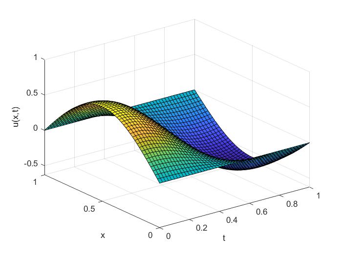
Figure 1. Behavior of the solution for the Riesz kernel with $\rho=1.75$.

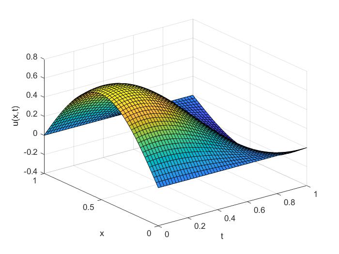
Figure 2. Behavior of the solution for the exponential kernel with $a=2$.

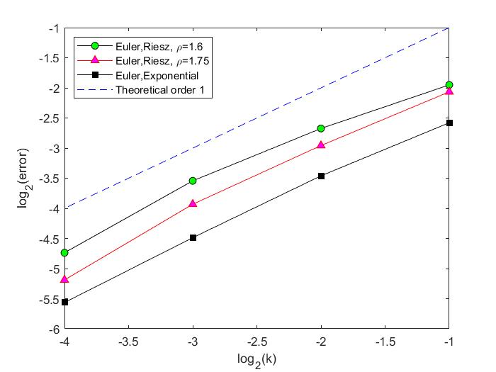
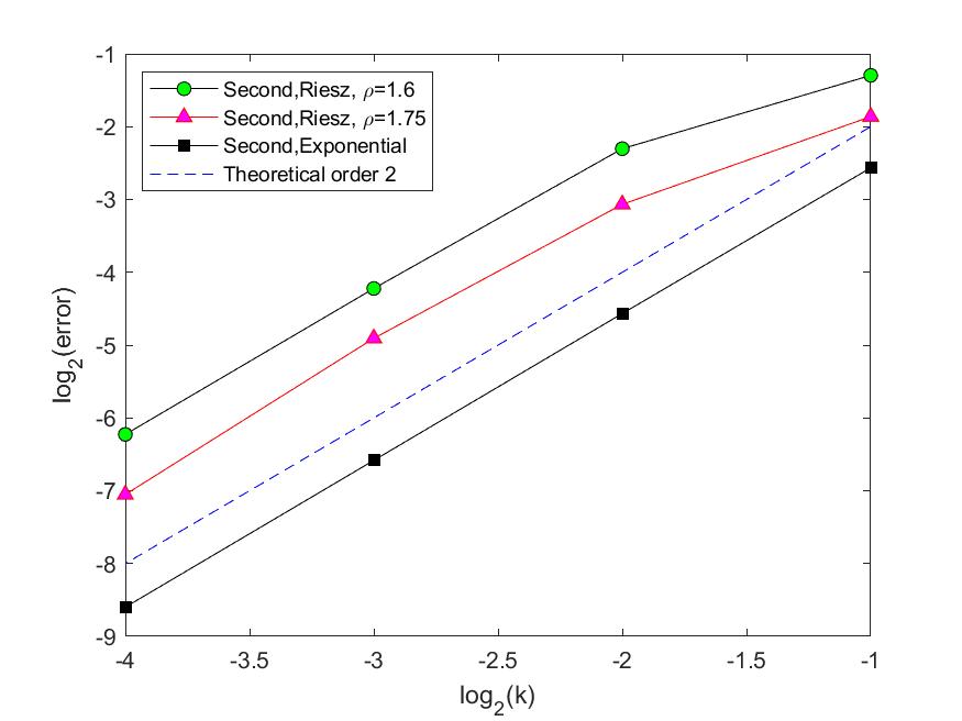
Figure 3. In the left panel, the temporal rate of convergence of the exponential Euler integrator applied to examples 6.1 and 6.2 is shown. In the right panel, the temporal rate of convergence of the second-order method is shown.

References

- [1] B. Baeumer, M. Geissert, and M. Kovács, Existence, uniqueness and regularity for a class of semilinear stochastic Volterra equations with multiplicative noise, J. Differential Equations. 258 (2015), pp. 535–554.
- [2] E. Cuesta, C. Lubich, C. Palencia, Convolution quadrature time discretization of fractional diffusion-wave equations, Mathematics of Computation, 254 (2006), pp. 673–696.
- [3] E. Cuesta and C. Palencia, A numerical method for an integro-differential equation with memory in Banach spaces: Qualitative properties, SIAM J. Numer. Anal. 41 (2003) pp. 1232–1241.
- [4] C. Cheng, V. Thomée, and L. Wahlbin, Finite element approximation of a parabolic integro-differential equation with a weakly singular kernel, Mathematics of Computation, 58 (1992), pp. 587–602.
- [5] R. Garrappa, A family of Adams exponential integrators for fractional linear systems, Computer and Mathematics with Applications, 66 (2013), pp. 717–727.
- [6] D. Henry, Geometric Theory of Semilinear Parabolic Equations, Lecture Notes in Math. 840, Springer, Berlin, Heidelberg, 1981.
- [7] M. Hochbruck and A. Ostermann, Explicit exponential Runge–Kutta methods for semilinear parabolic problems, SIAM J. Numer. Anal. 43 (2005), pp. 1069–1090.
- [8] M. Hochbruck and A. Ostermann, Exponential Runge–Kutta methods for parabolic problems, Appl. Numer. Math. 43 (2005), pp. 323–339.
- [9] M. Hochbruck and A. Ostermann, Exponential integrators, Acta Numerica, 19 (2010), pp. 209–286.
- [10] M. Kovács, S. Larsson, and F. Saedpanah, Mittag–Leffler Euler integrator for a stochastic fractional order equation with additive noise, SIAM J. Numer. Anal. 58 (2020), pp. 66–85.
- [11] A.-K. Kassam and L. N. Trefethen, Fourth-order time stepping for stiff PDEs, SIAM J. Sci. Comput., 26 (2005) , pp. 1214–1233.
- [12] S. Krogstad, Generalized integrating factor methods for stiff PDEs, J. Comput. Phys., 203 (2005), pp. 72–88.
- [13] C. Lubich and A. Ostermann, Linearly implicit time discretization of non-linear parabolic equations, IMA J. Numer. Anal. 15 (1995), pp. 555–583.
- [14] C. Lubich and A. Ostermann, Runge–Kutta approximation of quasi-linear parabolic equations, Math. Comp. 64 (1995), pp. 601–627.
- [15] C. Lubich, I. Sloan, and V. Thomée, Nonsmooth data error estimates for approximations of an evolution equation with a positive-type memory term, Mathematics of Computation, 65 (1996), pp. 1–17.
- [16] F. Mainardi and P. Paradisi, Fractional diffusive waves, J. Comput. Acoustics 9 (2001), pp. 1417–1436.
- [17] W. McLean and V. Thomée, Numerical solution of an evolution equation with positive memory term, J. Austral. Math. Soc. Ser. B, 35 (1993), pp. 23–70.
- [18] A. Pazy, Semigroups of Linear Operators and Applications to Partial Differential Equations, Applied Mathematical Sciences, Springer, 1983.
- [19] I. Podlubny, Fractional Differential Equations, Academic Press, San Diego, 1999.
- [20] I. Podlubny, Mittag–Leffler function (https://www.mathworks.com/matlabcentral/fileexchange/8738-mittag-leffler-function), MATLAB Central File Exchange. Retrieved January 22, 2023.
- [21] J. Prüss, Evolutionary Integral Equations and Applications. Monographs in Mathematics, vol. 87, Birkhäuser, Basel, 1993.
- [22] J. M. Sanz-Serna, A numerical method for a partial integro-differential equation, SIAM J. Numer. Anal. 25 (1988), pp. 319–327.