Efficient computational methods for rovibrational transition rates in molecular collisions

Abstract

Astrophysical modeling of processes in environments that are not in local thermal equilibrium requires the knowledge of state-to-state rate coefficients of rovibrational transitions in molecular collisions. These rate coefficients can be obtained from coupled-channel (CC) quantum scattering calculations which are very demanding, however. Here we present various approximate, but more efficient methods based on the coupled-states approximation (CSA) which neglects the off-diagonal Coriolis coupling in the scattering Hamiltonian in body-fixed coordinates. In particular, we investigated a method called NNCC (nearest-neighbor Coriolis coupling) [D. Yang, X. Hu, D. H. Zhang, and D. Xie, J. Chem. Phys. 148, 084101 (2018)] that includes Coriolis coupling to first order. The NNCC method is more demanding than the common CSA method, but still much more efficient than full CC calculations, and it is substantially more accurate than CSA. All of this is illustrated by showing state-to-state cross sections and rate coefficients of rovibrational transitions induced in CO₂ by collisions with He atoms. It is also shown that a further reduction of CPU time, practically without loss of accuracy, can be obtained by combining the NNCC method with the multi-channel distorted-wave Born approximation (MC-DWBA) that we applied in full CC calculations in a previous paper.

I Introduction

In modeling protoplanetary disks and other interstellar media that are not in local thermal equilibrium (LTE) with the aid of spectroscopic data from ground and satellite based telescopes pontoppidan:08 ; mandell:12 ; bruderer:15 ; bosman:17 ; bosman:19 , the effects of molecular collisions are important. In such non-LTE environments the populations of the rovibrational states of a molecule —and thereby the characteristics of its spectrum— are not only determined by absorption and emission of electromagnetic radiation, but also by transitions induced by molecular collisions. By analyzing these spectra one gets crucial information not only about the abundance of various molecules, but also about the local conditions. An essential element in this analysis is the knowledge of the rate coefficients of rovibrational transitions induced by the collisions of the molecule with H₂ molecules, He atoms, and electrons. Quantum scattering calculations, based on intermolecular potentials determined by ab initio electronic-structure calculations, can provide inelastic collision cross sections, from which the required transition rate coefficients and their temperature dependence can be derived.

An important molecule in these studies is carbon dioxide, CO₂ oberg:11 ; bosman:17 ; bosman:19 . Accurate cross sections and rate coefficients for rotationally inelastic CO₂-He collisions were recently reported by Godard Palluet et al. palluet:22 . CO₂ has no permanent dipole moment, so its rotational transitions are forbidden and it cannot be observed in microwave or far-infrared spectra. But it can be observed in mid- and near-infrared spectra through its vibrational transitions. It has three vibrational modes: a twofold degenerate bend mode with experimental frequency 667 cm^-1, an asymmetric stretch mode at 2349 cm^-1 , and a symmetric stretch mode at 1333 cm^-1. The latter mode is not infrared active by itself but becomes observable through a Fermi resonance with the bend overtone. In the pioneering theoretical studies of rate coefficients for vibrational transitions in CO₂ induced by collisions with rare gas (Rg) atoms by Clary et al. clary:81 ; clary:82 ; banks:87b ; wickham:87b they used VCC-IOS, a vibrational coupled-channel (CC) method for the vibrations, combined with the infinite-order sudden (IOS) approximation for the rotations. This method provided rate coefficients for vibrational transitions, without considering specific initial and final rotational states. The more advanced models currently being developed by astronomers bosman:17 ; bosman:19 and the availability of data from the James Webb space telescope (JWST) in the near future require rovibrational state-to-state collisional rate coefficients. These can nowadays be obtained from the numerically exact coupled-channel (CC) method with the use of accurate ab initio calculated intermolecular potentials. Full CC calculations are still time-consuming, however, especially at the higher collision energies needed to obtain rate coefficients for higher temperatures. In a previous paper selim:21 we have shown how one can reach the CC level of accuracy with a less time-consuming procedure that handles the coupling between rotational states by the CC method and the weaker coupling between different vibrational states with the multichannel distorted-wave Born approximation (MC-DWBA). Here we investigate further possibilities to speed up the calculation of collisional rate coefficients for rovibrational transitions by using the coupled-states approximation (CSA) and an improvement of it that includes Coriolis coupling to first order. We apply various methods to CO₂-He collisions with CO₂ excited in the symmetric stretch mode. We consider both the efficiency of these methods and the accuracy of the results they provide.

II Theory

II.1 Coupled channels method

The methods discussed in the present paper are based on the coupled-channels (CC) —also called close-coupling— method, formulated in body-fixed (BF) coordinates. These coordinates refer to a BF frame with its $z$-axis along the vector $\bm{R}$ that points from the center of mass of CO₂ to the He nucleus and the CO₂-He complex lying in the $xz$-plane. The coordinates are the length $R$ of the vector $\bm{R}$, the angle $\theta$ between the CO₂ axis and the vector $\bm{R}$, and the normal coordinate $Q$ along which CO₂ is deformed with respect to its linear equilibrium geometry with equal C-O bond lengths of 1.162 Å.

The 3D Hamiltonian of vibrotor-atom system CO₂-He over a monomer normal coordinate $Q$ is given, in the BF frame, by

$$\hat{H}=-\frac{\hbar^{2}}{2\mu R}\frac{\partial^{2}}{\partial R^{2}}R+\hat{H}_{\textrm{CO}_{2}}(Q)+\frac{\hat{J}^{2}+\hat{j}^{2}-2\hat{\bm{j}}\cdot\hat{\bm{J}}}{2\mu R^{2}}+V(Q,R,\theta),$$ (1)

where $\mu=m_{\textrm{CO}_{2}}m_{\textrm{He}}/(m_{\textrm{CO}_{2}}+m_{\textrm{He}})$ is the reduced mass of the complex, $\hat{\bm{j}}$ the CO₂ monomer rotational angular momentum operator, $\hat{\bm{J}}$ the total angular momentum operator of the complex, and $\hat{J}^{2}+\hat{j}^{2}-2\hat{\bm{j}}\cdot\hat{\bm{J}}$ represents the end-over-end angular momentum operator $L^{2}$ in the BF-frame avoird:94 . The monomer Hamiltonian $\hat{H}_{\textrm{CO}_{2}}(Q)$ is defined in Eq. (2) of Ref. selim:21 and also the computation of the normal modes $Q$ —its eigenstates in the rigid-rotor harmonic-oscillator approximation— is described there. Here we consider the symmetric stretch mode $Q\equiv Q_{1}=0.17678\Delta z_{1}-0.17678\Delta z_{3}$ $a_{0}$, where $\Delta z_{1}$ and $\Delta z_{3}$ are the displacements of the O atoms along the CO₂ axis with respect to their equilibrium positions. The symmetric stretch mode does not displace the C atom.

The eigenfunctions of the CO₂ monomer Hamiltonian are

$$|\mskip 3.0muvj\Omega\mskip 3.0mu\rangle=\chi_{vj}(Q)Y_{j\Omega}(\theta,\phi)$$ (2)

and the corresponding eigenvalues are $\epsilon_{vj}$. The vibrational functions $\chi_{vj}(Q)$ are $j$-dependent, the rotational functions $Y_{j\Omega}(\theta,\phi)$ are spherical harmonics. The latter are expressed with respect to the BF frame, the angle $\theta$ is the same as defined above and the angle $\phi$ coincides with the third Euler angle for the overall rotation of the complex. The quantum number $\Omega$ is the projection of the CO₂ angular momentum $\hat{\bm{j}}$ and of the total angular momentum $\hat{\bm{J}}$ on the BF $z$-axis along the vector $\bm{R}$.

The channel basis in coupled channels (CC) scattering calculations for rovibrationally inelastic CO₂-He collisions is, in BF coordinates,

$$|\mskip 3.0muvj\Omega;JM_{J}\mskip 3.0mu\rangle=\sqrt{\frac{2J+1}{4\pi}}\chi_{vj}(Q)Y_{j\Omega}(\theta,0)D^{J}_{M_{J}\Omega}(\alpha,\beta,\phi)^{*}.$$ (3)

The angles $(\beta,\alpha)$ are the polar angles of the vector $\bm{R}$ with respect to a space-fixed frame (SF), and the Euler angles $(\alpha,\beta,\phi)$ in the Wigner $D$-functions describe the orientation of the BF frame relative to the SF frame. The angle $\phi$ has been moved from the spherical harmonics in Eq. (2) to the overall rotation functions, which is mathematically equivalent.

The Coriolis coupling operator $2\hat{\bm{j}}\cdot\hat{\bm{J}}$ in Eq. (1) can be written as

$$2\hat{\bm{j}}\cdot\hat{\bm{J}}=2\hat{j}_{z}\hat{J}_{z}+\hat{j}_{+}\hat{J}_{+}+\hat{j}_{-}\hat{J}_{-}.$$ (4)

The so-called helicity quantum number $\Omega$ is an eigenvalue of both $\hat{j}_{z}$ and $\hat{J}_{z}$. It is an approximate quantum number; basis functions with different $\Omega$ are mixed by the ladder operators $\hat{j}_{\pm}\hat{J}_{\pm}$ in Eq. (4) which couple functions with $\Omega$ to those with $\Omega\pm 1$.

Also the ab initio calculation of the 3D CO₂-He potential with CO₂ deformed along the symmetric stretch coordinate $Q_{1}$ is described in Ref. selim:21 . The well depth of this potential for CO₂ at its equilibrium geometry is 47.43 cm^-1. When this potential is expanded in Legendre polynomials $P_{\lambda}(\cos\theta)$ of order $\lambda$, as in Ref. selim:21

$$V(Q,R,\theta)=\sum_{\lambda}C_{\lambda}(Q,R)P_{\lambda}(\cos\theta),$$ (5)

its matrix elements over the BF basis are

$$V_{v^{\prime}j^{\prime}\Omega^{\prime};vj\Omega}(R) = \langle\mskip 3.0muv^{\prime}j^{\prime}\Omega^{\prime};JM_{J}\mskip 3.0mu|\mskip 3.0muV(Q,R,\theta)\mskip 3.0mu|\mskip 3.0muvj\Omega;JM_{J}\mskip 3.0mu\rangle$$ (6)

$$= \delta_{\Omega^{\prime}\Omega}\;\sum_{\lambda}(-1)^{\Omega^{\prime}}[(2j^{\prime}+1)(2j+1)]^{1/2}\begin{pmatrix}j^{\prime}&\lambda&j\\ 0&0&0\end{pmatrix}\begin{pmatrix}j^{\prime}&\lambda&j\\ -\Omega&0&\Omega\end{pmatrix}$$

$$\times\langle\mskip 3.0muv^{\prime}j^{\prime}(Q)\mskip 3.0mu|\mskip 3.0muC_{\lambda}(Q,R)\mskip 3.0mu|\mskip 3.0muvj(Q)\mskip 3.0mu\rangle.$$

Equation (6) shows the advantages of the BF basis: the potential $V(Q,R,\theta)$ does not couple functions with different $\Omega$ and the expression for its remaining matrix elements is simpler than in the SF basis arthurs:60 , which makes the calculations more efficient.

The overall angular momentum $J$ and its projection $M_{J}$ on the SF $z$-axis are exact quantum numbers and also the overall parity $P$ under inversion of the system is a conserved quantity. The basis in Eq. (3) is not invariant under inversion; a parity adapted basis is

$$|\mskip 3.0muvj\tilde{\Omega};PJM_{J}\mskip 3.0mu\rangle=\left[|\mskip 3.0muvj\,\tilde{\Omega};PJM_{J}\mskip 3.0mu\rangle+P(-1)^{J}|\mskip 3.0muvj\,{-\tilde{\Omega}};PJM_{J}\mskip 3.0mu\rangle\right]/\sqrt{2(1+\delta_{\tilde{\Omega}\,0})},$$ (7)

where $\tilde{\Omega}\geq 0$ and $P=\pm 1$ is the overall parity.

Another valid symmetry operation is the interchange $P_{13}$ of the O atoms in CO₂. This operator affects only the monomer wave functions in the basis of Eq. (3). For the symmetric stretch mode that we consider here, we find

$$\hat{P}_{13}|\mskip 3.0muvj\tilde{\Omega}\mskip 3.0mu\rangle=(-1)^{j}|\mskip 3.0muvj\tilde{\Omega}\mskip 3.0mu\rangle$$ (8)

Since ¹⁶O nuclei are bosons with spin zero, the wave functions must be symmetric under $\hat{P}_{13}$. This implies that only functions with even $j$ are allowed.

The scattering wave functions in CC calculations are written in terms of the parity-adapted BF channel basis as

$$\Psi^{PJM_{J}}=\frac{1}{R}\sum_{vj\tilde{\Omega}}|\mskip 3.0muvj\tilde{\Omega};PJM_{J}\mskip 3.0mu\rangle\psi^{PJM_{J}}_{vj\tilde{\Omega}}(R).$$ (9)

When these functions are substituted into the time-independent Schrödinger equation, it follows that the radial wave functions $\psi^{PJ}_{vj\tilde{\Omega}}(R)$ must obey a set of coupled second order differential equations, the CC equations

$$\frac{\partial^{2}}{\partial R^{2}}\psi^{PJ}_{v^{\prime}j^{\prime}\tilde{\Omega}^{\prime}}(R)=\sum_{vj\tilde{\Omega}}W_{v^{\prime}j^{\prime}\Omega^{\prime};vj\Omega}^{PJ}(R)\psi_{vj\tilde{\Omega}}^{PJ}(R),$$ (10)

or in matrix form

$$\bm{\psi}^{\prime\prime}(R)={\bm{W}}(R)\bm{\psi}(R).$$ (11)

The column vector $\bm{\psi}(R)$ contains the radial wave functions $\psi^{PJ}_{vj\tilde{\Omega}}(R)$. The quantum number $M_{J}$ has been omitted, since the solutions do not depend on it. The elements of the matrix ${\bm{W}}$ over the primitive basis in Eq. (3) are given by

$$W_{v^{\prime}j^{\prime}\Omega^{\prime};vj\Omega}^{J}(R)=-\delta_{v^{\prime}v}\delta_{j^{\prime}j}\delta_{\Omega^{\prime}\Omega}k_{vj}^{2}+T_{v^{\prime}j^{\prime}\Omega^{\prime};vj\Omega}^{J}(R)+2\mu V_{v^{\prime}j^{\prime}\Omega^{\prime};vj\Omega}(R),$$ (12)

with

$$k_{vj}^{2}=2\mu(E-\epsilon_{vj}),$$ (13)

and $E$ being the total energy. The matrix elements of the potential are defined in Eq. (6); this matrix is diagonal in $\Omega$. Only the matrix ${\bm{T}}$ which originates from the angular kinetic energy operator is not diagonal in $\Omega$. Its elements are

$$T_{v^{\prime}j^{\prime}\Omega^{\prime};vj\Omega}^{J}(R)= R^{-2}\delta_{v^{\prime}v}\delta_{j^{\prime}j}\Big{\{}\delta_{\Omega^{\prime}\Omega}\left[J(J+1+j(j+1)-2\Omega^{2}\right]\Big{.}$$ (14)

$$\Big{.}-\delta_{\Omega^{\prime}\Omega\pm 1}\left[J(J+1-\Omega(\Omega\pm 1)\right]^{1/2}\left[j(j+1-\Omega(\Omega\pm 1)\right]^{1/2}\Big{\}}$$

So ${\bm{T}}$, and therefore also ${\bm{W}}$, contains a series of blocks diagonal in $\Omega$ and a series of neighboring blocks with $\Omega^{\prime}=\Omega\pm 1$. All other elements of these matrices are zero, thanks to the use of a BF basis in which the potential matrix $\bm{V}$ is diagonal in $\Omega$.

We solve these equations with the renormalized Numerov propagator method johnson:78 ; johnson:79 . This method implies that one defines an equidistant grid $R_{i},i=1,\ldots,n$ and propagates the matrix ${\bm{Q}}$, which defines the ratio of the radial wave functions in subsequent grid points $R_{i-1}$ and $R_{i}$

$$\bm{\psi}(R_{i-1})={\bm{Q}}_{i}\bm{\psi}(R_{i}).$$ (15)

The propagation starts at small $R_{1}$, where the potential is sufficiently repulsive that the wave function —and therefore ${\bm{Q}}$— is zero, and continues to large $R_{n}$, where the potential has vanished. Then, we assume that the radial wave functions obey flux-normalized $K$-matrix boundary conditions at large $R$

$$\bm{\psi}(R)={\bm{F}}(R)-{\bm{G}}(R){\bm{K}}.$$ (16)

The symbol $\bm{\psi}(R)$ is here used for a matrix with column vectors that are the solutions of the CC equations in Eq. (11). The blocks of the matrices ${\bm{F}}(R)$ and ${\bm{G}}(R)$ for the open channels are diagonal

$$F_{v^{\prime}j^{\prime}L^{\prime};vjL}(R) = \delta_{v^{\prime}j^{\prime};vj}\;\delta_{L^{\prime}L}\;k_{vj}^{1/2}\,R\,j_{L}(k_{vj}R)$$

$$G_{v^{\prime}j^{\prime}L^{\prime};vjL}(R) = \delta_{v^{\prime}j^{\prime};vj}\;\delta_{L^{\prime}L}\;k_{vj}^{1/2}\,R\,y_{L}(k_{vj}R),$$ (17)

and contain asymptotic wave functions that are proportional to spherical Riccati-Bessel functions abramowitz:64 of the first and second kind $j_{L}(z)=\sqrt{\frac{1}{2}\pi/z}J_{L+\frac{1}{2}}(z)$ and $y_{L}(z)=\sqrt{\frac{1}{2}\pi/z}Y_{L+\frac{1}{2}}(z)$. Similarly, closed channels are matched to modified spherical Bessel functions of the first and second kind $I_{L+\frac{1}{2}}(z)$ and $K_{L+\frac{1}{2}}(z)$, respectively, which occur in off-diagonal blocks of the matrices ${\bm{F}}(R)$ and ${\bm{G}}(R)$.

The asymptotic wave functions are defined in the SF frame and depend on the partial wave index $L$, while the matrix ${\bm{Q}}_{n}$ is obtained from the propagation in BF coordinates. Therefore, this matrix is first transformed to SF coordinates

$${\bm{Q}}^{\textrm{SF}}_{n}={\bm{U}}^{\dagger}{\bm{Q}}_{n}{\bm{U}}.$$ (18)

The elements of ${\bm{U}}$

$$U^{Jj}_{\Omega L}=\langle\mskip 3.0muj\Omega L0\mskip 3.0mu|\mskip 3.0muJ\Omega\mskip 3.0mu\rangle\sqrt{\frac{2L+1}{2J+1}}$$ (19)

contain Clebsch-Gordan coefficients $\langle\mskip 3.0mu....\mskip 3.0mu|\mskip 3.0mu..\mskip 3.0mu\rangle$ selim:21 . The matrix ${\bm{K}}$ can then be obtained from ${\bm{Q}}^{\textrm{SF}}_{n}$ by solving the linear equations

$$\Big{[}{\bm{G}}(R_{n-1})-{\bm{Q}}^{\textrm{SF}}_{n}{\bm{G}}(R_{n})\Big{]}{\bm{K}}={\bm{F}}(R_{n-1})-{\bm{Q}}^{\textrm{SF}}_{n}{\bm{F}}(R_{n}).$$ (20)

Finally, we use the open-channel block $\bm{K}_{\rm oo}$ of the matrix $\bm{K}$ to obtain the scattering matrix

$${\bm{S}}=({\bm{I}}-i{\bm{K}}_{\rm oo})^{-1}(I+i{\bm{K}}_{\rm oo}),$$ (21)

with ${\bm{I}}$ being the unit matrix, and compute state-to-state scattering cross sections

$$\sigma_{v^{\prime},j^{\prime}\leftarrow v,j}(E)=\frac{\pi}{(2{j}+1)k^{2}_{vj}}\sum_{P\,J}(2J+1)\sum_{L^{\prime}=|J-j^{\prime}|}^{J+j^{\prime}}\sum_{L=|J-j|}^{J+j}\left|\delta_{v^{\prime}v}\delta_{j^{\prime}j}\delta_{L^{\prime}L}-S^{P\,J}_{v^{\prime}j^{\prime}L^{\prime};vjL}(E)\right|^{2}.$$ (22)

Expressions for the temperature ($T$) dependent rate coefficients $k_{v^{\prime},j^{\prime}\leftarrow v,j}(T)$ of the transitions from rovibrational state $v,j$ to state $v^{\prime},j^{\prime}$ are given in Ref. selim:21 . Since the total angular momentum $J$ and the overall parity $P$ are exact quantum numbers, the CC equations can be solved separately for parities $P=\pm 1$ and for all values of $J$ required to obtain converged cross sections.

II.2 Coupled states approximation

In the coupled-states approximation (CSA), introduced long ago mcguire:74 , one neglects the Coriolis coupling terms off-diagonal in $\Omega$ that appear in the second line of Eq. (14). This makes $\Omega$ an exact quantum number, so that the CC equations can be separated into subsets of equations for each value of $\Omega$. The dimension of each subset is smaller by a factor of $\min(2J+1,2j_{\rm max}+1)$, where $j_{\rm max}$ is the maximum $j$-value in the basis, than the dimension of the full CC equations. Since the CPU time to solve the coupled equations is proportional to the third power of their dimension, this yields a large reduction in computer time. Moreover, since different $\Omega$ values are not coupled, the largest absolute value of $\Omega$ is limited to the smallest of the initial or final $j$ value in the scattering process, which is smaller than $j_{\rm max}$ —and also much smalller than $J$ in most cases— so the number of equation subsets to be solved is small also.

In the standard application of the CSA the whole angular kinetic operator in Eq. (4) is replaced by an operator $\hat{L}^{2}$, with eigenvalues $L_{\rm eff}(L_{\rm eff}+1)$. The possible values of $L$ range from $|J-j|$ to $J+j$, and different choices of $L_{\rm eff}$ have been investigated. One mostly uses $L_{\rm eff}=J$, which yields an angular kinetic energy proportional to $J(J+1)$. In our BF implementation with the renormalized Numerov propagator we have three different options. First, we can follow the original CSA algorithm by using $L_{\rm eff}=J$ also in the matching of the asymptotic scattering wave functions to obtain the scattering matrices ${\bm{S}}^{P\,J\,\Omega}$ for all values of $P$, $J$, and $\Omega$. The cross sections can then be obtained from the equation

$$\sigma_{v^{\prime},j^{\prime}\leftarrow v,j}(E)=\frac{\pi}{(2{j}+1)k^{2}_{vj}}\sum_{P\,J\,\Omega}(2J+1)\left|\delta_{v^{\prime}v}\delta_{j^{\prime}j}-S^{PJ\Omega}_{v^{\prime}j^{\prime};vj}(E)\right|^{2}.$$ (23)

Instead of using each of the matrices ${\bm{Q}}_{n}^{\Omega}$ obtained after solving the coupled-states equations for different $\Omega$ values directly in an asymptotic matching procedure that yields matrices ${\bm{S}}^{P\,J\,\Omega}$, one may follow an alternative procedure. This alternative implies that the individual matrices ${\bm{Q}}_{n}^{\Omega}$ are collected into a total matrix ${\bm{Q}}_{n}$, which consists of diagonal subblocks with the matrices ${\bm{Q}}_{n}^{\Omega}$ for all $\Omega$ values. All other elements of ${\bm{Q}}_{n}$ are zero, since in CSA there is no coupling between functions with different $\Omega$. Since this total ${\bm{Q}}_{n}$ matrix involves the full BF channel basis containing all values of $\Omega$, it can be transformed to its SF equivalent in the same way as in the full CC treatment, see Eq. (18). It can then be used in the same asymptotic matching procedure as described in Sec. II.1 to obtain the scattering matrices ${\bm{S}}^{P\,J}$ that occur in Eq. (22) for the cross sections. In the propagation of the individual matrices ${\bm{Q}}_{i}^{\Omega}$ with $i=1,\ldots,n$ one may either use the full diagonal angular kinetic energy $\big{[}J(J+1)+j(j+1)-2\Omega^{2}\big{]}/2\mu R^{2}$ from the first line of Eq. (14) or an effective angular kinetic energy $L_{\rm eff}(L_{\rm eff}+1)=J(J+1)$ as in the original CSA method. Altogether, this yields three different variants of the CSA, of which we compare the results in Sec. III. In the figures we label these variants with $L_{\rm eff}=J$ for the standard CSA application, and with the angular kinetic energies $\big{[}J(J+1)+j(j+1)-2\Omega^{2}\big{]}/2\mu R^{2}$ and $J(J+1)$ that we take into account in the latter two CSA methods.

II.3 Improving the coupled-states approximation with first-order Coriolis coupling

The error in the CSA relative to full CC calculations is sometimes not acceptable. Recently Yang et al. yang:18 introduced an improvement of the CSA method, called NNCC, which includes the Coriolis coupling between functions with $\Omega$ and $\Omega\pm 1$ to first order. It implies that the CC equations are still solved separately for each $\Omega$ value, but with the off-diagonal Coriolis couplings to the neighboring blocks with $\Omega\pm 1$ included in the matrix ${\bm{W}}$, cf. Eqs. (12) and (14). In the full CC equations these neighboring blocks are again coupled to functions with $\Omega\pm 2$, but the latter are not directly coupled to the functions with the given $\Omega$, so they only give rise to second and higher order contributions to the solutions. The NNCC method neglects these higher order Coriolis couplings.

The basis to solve the CC equations for each $\Omega$ in the NNCC method involves also the bases for $\Omega-1$ and $\Omega+1$. The propagation can then be done with the full angular kinetic energy from Eq. (14). Functions with different $\Omega$ are coupled by the off-diagonal Coriolis coupling terms in the second line of this equation, which has the effect that $\Omega$ is not a good quantum number anymore. We could still label the separate propagations with $\Omega$, but in order to distinguish the individual propagations from the quantum numbers, we label them with the index $\overline{\Omega}$. The propagation does not have to be performed for all $\Omega$ values, because the $\Omega=0$ basis is already included in the calculation for the parity-adapted basis with $\tilde{\Omega}=1$, see Eq. (7), and the $\tilde{\Omega}=J$ basis is included in the calculation for $\tilde{\Omega}=J-1$. Also in the NNCC method the calculations can be further restricted to $\tilde{\Omega}$ values limited by the smallest of the initial and final $j$ quantum numbers, augmented by one in this case. At the end of the propagations we have two options. The first one is that we follow the NNCC method as proposed by Yang et al. yang:18 . At the end of each propagation $\overline{\Omega}$ they construct an equivalent SF basis by diagonalizing the operator $\hat{L}^{2}$ with the BF matrix elements from Eq. (14) in the space of functions $\Omega-1$, $\Omega$, and $\Omega+1$. The eigenvalues $L(L+1)$ from this diagonalization are non-integer, and also $L$ is therefore non-integer. The same procedure has been implemented previously in the reactive scattering program ABC skouteris:00 , which has the possibility to truncate the $\Omega$ basis. The matrix ${\bm{B}}^{\overline{\Omega}}$ with the eigenvectors of $\hat{L}^{2}$ in the restricted $\Omega$ space as column vectors is then used to transform the matrix ${\bm{Q}}_{n}^{\overline{\Omega}}$ obtained at the end of propagation $\overline{\Omega}$ to its SF equivalent

$${\bm{Q}}^{\overline{\Omega},\textrm{SF}}_{n}={{\bm{B}}^{\overline{\Omega}}}^{\,\dagger}{\bm{Q}}_{n}^{\overline{\Omega}}{\bm{B}}^{\overline{\Omega}}.$$ (24)

This numerical diagonalization of $\hat{L}^{2}$ leaves the overall sign of each eigenvector, i.e., of each column of the matrix ${\bm{B}}^{\overline{\Omega}}$, undetermined. This has no effect on the final results, however, because the inverse of ${\bm{B}}^{\overline{\Omega}}$ is used in Eq. (25) to transform the $S$-matrix back from the SF to the BF frame. Indeed, we found numerically that the final cross sections in Eq. (26) do not depend on these signs. Since the SF basis thus obtained corresponds to non-integer $L$ values, the spherical Bessel functions used in the matching procedure described in Eqs. (16) to (20) must be the corresponding functions with non-integer $L$ values abramowitz:64 .

The second option is that we consider the matrices ${\bm{Q}}^{\overline{\Omega}}_{n}$ over the BF basis with $\Omega-1$, $\Omega$, and $\Omega+1$ as part of the matrix ${\bm{Q}}_{n}$ over the full BF basis and transform them to the SF basis with the aid of Eq. (18). The transformation matrix ${\bm{U}}$ contains Clebsch-Gordan coefficients, the $L$ values are integers, and the asymptotic matching procedure to obtain SF matrices ${\bm{S}}^{{PJ\overline{\Omega}(\textrm{SF}})}$ from each propagation $\overline{\Omega}$ can be done with the usual spherical Bessel functions.

Finally, in both options, one has to transform the matrices ${\bm{S}}^{PJ\overline{\Omega}\,(\textrm{SF})}$ in the SF basis back to the BF basis with the aid of the inverse BF to SF transformation. In the first option, this transformation is done with the matrix ${\bm{B}}^{\overline{\Omega}}$ for the given $\overline{\Omega}$. Since ${\bm{B}}^{\overline{\Omega}}$ is a real orthogonal matrix, its inverse is simply its transpose and one obtains

$$S^{PJ\overline{\Omega}(\textrm{BF})}_{v^{\prime}j^{\prime}\Omega^{\prime};vj\Omega}=\sum_{L^{\prime}L}i^{L-L^{\prime}}B^{\overline{\Omega}}_{\Omega^{\prime}L^{\prime}}S^{PJ\overline{\Omega}(\textrm{SF})}_{v^{\prime}j^{\prime}L^{\prime};vjL}B^{\overline{\Omega}}_{L\Omega}$$ (25)

In the second option, the BF to SF transformation is done with the matrix ${\bm{U}}$ from Eq. (18), which is also orthogonal, and one obtains the same formula, with ${\bm{B}}^{\overline{\Omega}}$ replaced by ${\bm{U}}$. In order to avoid double counting, we select from each matrix ${\bm{S}}^{PJ\overline{\Omega}\,\textrm{BF}}$ only the blocks with $\Omega=\overline{\Omega}$ and calculate the cross sections with the formula

$$\sigma_{v^{\prime},j^{\prime}\leftarrow v,j}(E)=\frac{\pi}{(2{j}+1)k^{2}_{vj}}\sum_{\Omega}\sum_{\Omega^{\prime}=\Omega-1}^{\Omega+1}\sum_{P\,J\,\Omega}(2J+1)\left|\delta_{v^{\prime}v}\delta_{j^{\prime}j}-S^{PJ\overline{\Omega}(\textrm{BF})}_{v^{\prime}j^{\prime}\Omega^{\prime};vj\Omega}(E)\right|^{2}.$$ (26)

II.4 Combining NNCC with the multi-channel distorted wave Born approximation

In a previous paper selim:21 we have shown how the application of a multi-channel distorted wave Born approximation (MC-DWBA) in scattering calculations reduces the computer time by about a factor of three with respect to exact CC calculations, but produces cross sections and rate coefficients for rovibrational transitions in CO₂-He collisions that are about equally accurate. The MC-DWBA algorithm and the reason why it can be favorably applied to rovibrational transitions are explained in detail in Ref. selim:21 . Here we investigate the application of this algorithm in combination with the NNCC method.

II.5 Computational details

We study state-to-state ($v,j\rightarrow v^{\prime},j^{\prime}$) rovibrational transitions in CO₂ by collisions with He in which CO₂ is de-excited from the $v=1$ symmetric stretch fundamental to the $v^{\prime}=0$ ground state. The details of the calculation and the characteristics of the 3D intermolecular potential of CO₂-He with CO₂ deformed along the symmetric stretch coordinate are given in Ref. selim:21, . The basis in the scattering calculations consisted of CO₂ symmetric stretch functions with $v=0$ and 1, the rotational basis contained all functions with $j\leq 70$, for both $v=0$ and 1. Calculations were made with a larger vibrational basis including also $v=2$ functions, but this made practically no difference for the results. It is interesting that the states with $v,j=1,0$ and $v,j=0,58$ have nearly the same energy, so that transitions between these states are nearly resonant. The radial grid for the renormalized Numerov propagator contained 502 equidistant points in the range $3\leq R\leq 30~{}a_{0}$. Rovibrational state-to-state cross sections were calculated for collision energies up to 3000 cm^-1, with steps of 0.1 cm^-1 in the resonance regime from $1\leq E\leq 20$ cm^-1, steps of 1 cm^-1 for $20\leq E\leq 50$ cm^-1, 2 cm^-1 for $50\leq E\leq 100$ cm^-1, 50 cm^-1 for $100\leq E\leq 1000$ cm^-1, and 200 cm^-1 for $1000\leq E\leq 3000$ cm^-1. The largest total $J$ value included was 100, for both parities $P=\pm 1$. The corresponding rate coefficients were calculated for temperatures from 10 to 500 K by cubic spline interpolating the cross sections over the energy grid and calculating the integral in Eq. (14) of Ref. selim:21, with the trapezoidal rule. Since the rotational states of CO₂ up to $j=50$ with energy 991 cm^-1 are populated at the highest temperature, we calculated the cross sections and rate coefficients for initial states up to this value of $j$.

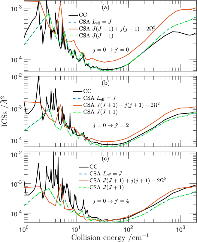
Figure 1: ICSs from the three different CSA methods described in Sec. II.2 compared with full CC results. The upper legend CC refers to ICSs from full CC calculations. The next legend CSA $L_{\rm eff}=J$ refers to the conventional CSA method with angular kinetic energy $L_{\rm eff}(L_{\rm eff}+1)$ and $L_{\rm eff}=J$ in which the ICS is calculated directly from the S-matrices for different $\Omega$ in the BF frame. The lower two legends refer to the CSA methods with angular kinetic energy terms $J(J+1)+j(j+1)-2\Omega^{2}$ or $J(J+1)$ used in the BF propagation and the ICS obtained from the $S$-matrix in the SF frame, after transformation of the BF matrix ${\bm{Q}}_{n}$ to the SF frame with the aid of Eq. (18). The initial state is $v=1,j=0$, the final states are $v^{\prime}=0$ with $j^{\prime}=0$ (a), $j^{\prime}=2$ (b), and $j^{\prime}=4$ (c).

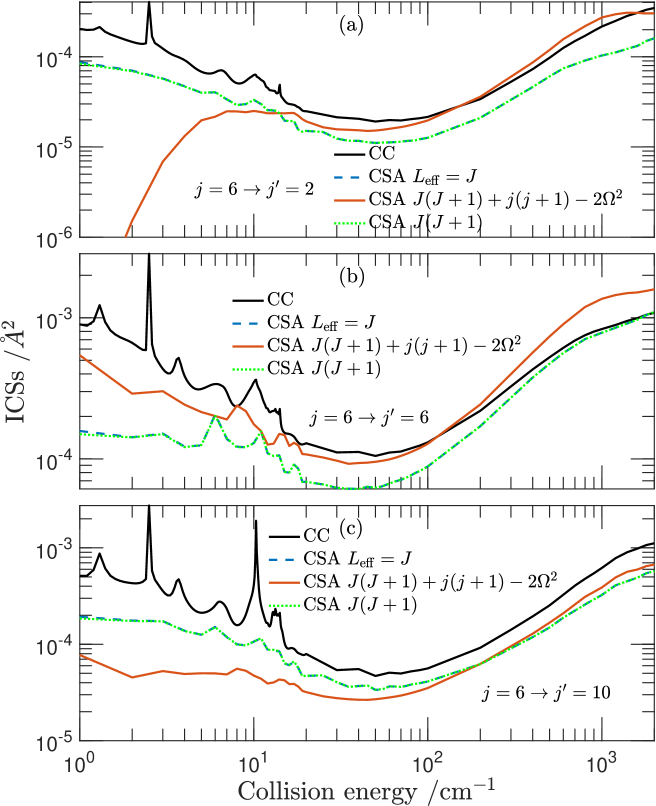
Figure 2: Same as Fig. 1, with a different initial state: $v=1,j=6$ and final states $v^{\prime}=0$ with $j^{\prime}=2$ (a), $j^{\prime}=6$ (b), and $j^{\prime}=10$ (c).

III Results and discussion

Figures 1 and 2 show the integral cross sections (ICSs) from the three different CSA methods described in Sec. II.2, in comparison with ICSs from full CC calculations, for quenching from initial state $v,j=1,0$ to different final states $v^{\prime}=0,j^{\prime}$. The meaning of the legends referring to the different CSA methods is explained in the caption of the figure. The sharp peaks in the ICSs for collision energies below 20 cm^-1 correspond to resonances, which are extremely sensitive to the details of the calculations. Hence, it is not surprising that they are different for the different scattering methods used. But also for higher energies one observes that the ICSs from the CSA methods differ substantially from the full CC results. Two of the CSA methods produce very similar results. In both of them the propagation is done in the BF frame with the angular kinetic energy term $J(J+1)$, but the asymptotic matching procedures to obtain the $S$-matrix are different, see Sec. II.2. Apparently, the way of matching is less important than the approximation in the angular kinetic energy term used in the propagation. The third CSA method, with the angular kinetic energy term $J(J+1)+j(j+1)-2\Omega^{2}$ produces rather different ICSs. The deviations of the CSA ICSs from the CC results are rather erratic, and one cannot conclude that one of the CSA methods is definitely better than the others. The method with the term $J(J+1)+j(j+1)-2\Omega^{2}$ contains the full angular kinetic energy when neglecting the Coriolis coupling between basis functions with different $\Omega$, so in the following we will show the results from this particular CSA approximation.

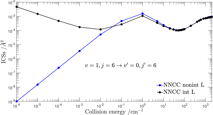
Figure 3: Comparison of ICSs calculated with the two different NNCC methods described in Sec. II.3. They differ in the asymptotic matching procedure using integer $L$ or non-integer $L$ values.

Figure 3 illustrates the effect of the different asymptotic matching procedures used in the NNCC methods described in Sec. II.3. In the method proposed by Yang et al. yang:18 they numerically determine the eigenvectors of the operator $\hat{L}^{2}$ in the BF basis restricted to a given $\Omega$ and $\Omega\pm 1$, which yields non-integer eigenvalues and, hence, non-integer $L$ values. These non-integer $L$ values are then used in the asymptotic matching procedure that yields the $S$-matrix. In the second method, we use specific rows of the matrix ${\bm{U}}$ from Eq. (19) that transforms the full BF basis to the SF basis. This full BF basis corresponds to a SF basis with integer $L$ values, which are used in the asymptotic matching procedure. Figure 3 shows that the ICSs from the two methods are very similar for collision energies higher than about 10 cm^-1. For lower energies, between 0.1 and 10 cm^-1, they become different, but this is the resonance regime where the ICSs are very sensitive to details of the potential and the computational method. The difference becomes very large for still lower energies approaching the Wigner regime. In this regime the ICSs of inelastic collisions should depend on $E^{-1/2}$ according to the Wigner threshold laws wigner:48 . The method with integer $L$ values nicely obeys this relation, but the method with non-integer $L$ values fails completely. This is not surprising, because the Wigner threshold law wigner:48 assumes pure $s$-wave scattering at the limit of very low energies, which implies that $L=0$. Only the method with integer $L$ correctly reaches this limit.

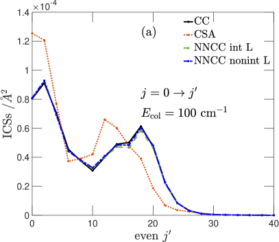
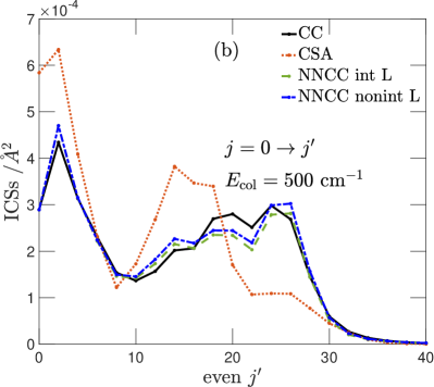
Figure 4: Product ($v^{\prime}=0,j^{\prime}$) distributions from the NNCC methods with integer and non-integer $L$ values for initial state $v=1,j=0$, compared with CSA and full CC calculations, at collision energies $E=100$ cm^-1 (a) and 500 cm^-1 (b). Note that only even values of $j$ and $j^{\prime}$ are physically allowed. The CSA method contains the angular kinetic energy $J(J+1)+j(j+1)-2\Omega^{2}$.

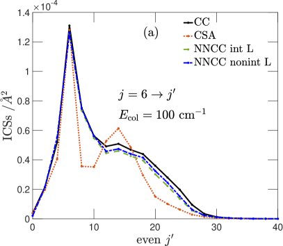
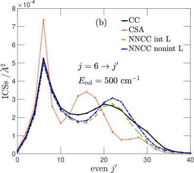
Figure 5: Same as Fig. 4 for initial state $v=1,j=6$ at collision energies $E=100$ cm^-1 (a) and 500 cm^-1 (b).

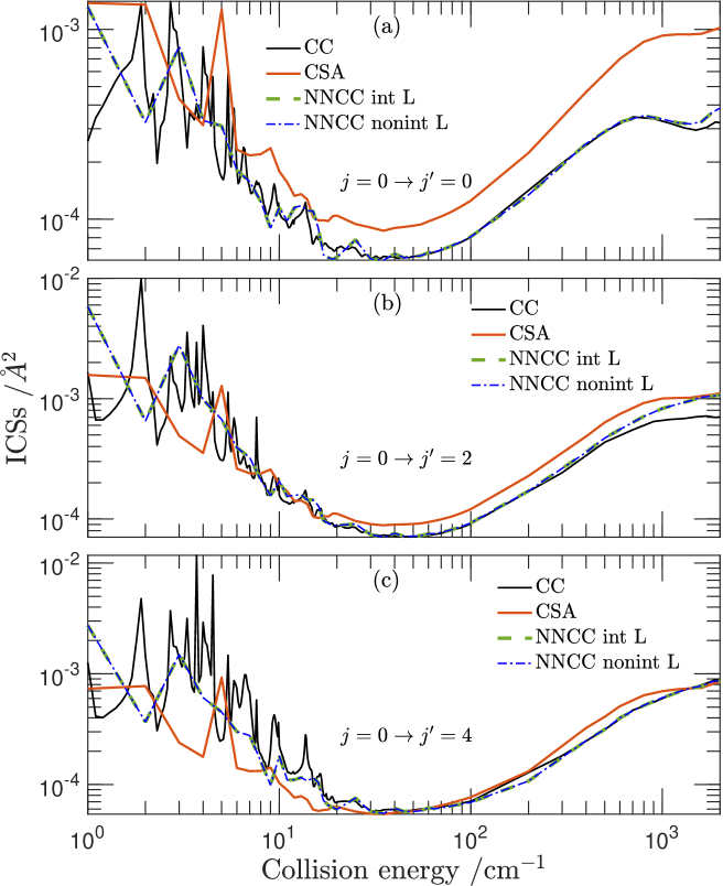
Figure 6: ICSs from the NNCC methods with integer and non-integer $L$ values described in Sec. II.3 compared with CSA and full CC results. The ICSs are shown as functions of the collision energy $E$ for initial state $v=1,j=0$ and final states $v^{\prime}=0,j^{\prime}=0$ (a), $v^{\prime}=0,j^{\prime}=2$ (b), and $v^{\prime}=0,j^{\prime}=4$ (c). The CSA method contains the angular kinetic energy $J(J+1)+j(j+1)-2\Omega^{2}$.

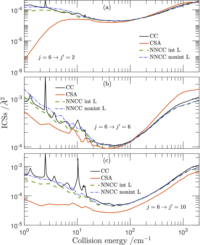
Figure 7: Same as Fig. 6 for initial state $v=1,j=6$ and final states $v^{\prime}=0,j^{\prime}=2$ (a), $v^{\prime}=0,j^{\prime}=6$ (b), and $v^{\prime}=0,j^{\prime}=10$ (c).

Figures 4 and 5 show product distributions from the NNCC methods with integer and non-integer $L$ values as described in Sec. II.3, for different initial states and different collision energies, compared with results from CSA and full CC calculations. A similar comparison is made in Figs. 6 and 7, which show the ICSs for the same initial $v=1,j$ values and specific final $v^{\prime}=0,j^{\prime}$ values as functions of the collision energy. It is obvious from all these figures that the NNCC method, which includes the first-order Coriolis coupling between basis functions with $\Omega$ and $\Omega\pm 1$, produces results in much better agreement with full CC calculations than the CSA methods. The NNCC methods with integer and non-integer $L$ values perform quite similarly. Except, of course, for collision energies below 0.1 cm^-1 displayed in Fig. 3, where the NNCC method with integer $L$ values becomes better because it obeys the Wigner threshold law, as discussed above.

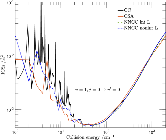
Figure 8: ICSs for quenching from initial state $v=1,j=0$ to the $v^{\prime}=0$ state, summed over all final $j^{\prime}$ values. The different curves are results from the NNCC methods with integer and non-integer $L$ values, compared with CSA and full CC results. The CSA method contains the angular kinetic energy $J(J+1)+j(j+1)-2\Omega^{2}$.

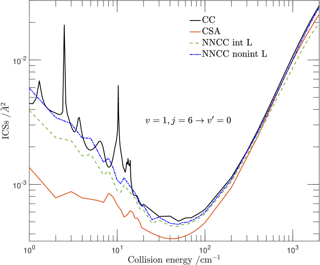
Figure 9: Same as Fig. 8 for initial state $v=1,j=6$.

In Figs. 8 and 9 we display the total quenching cross sections for transitions from initial states $v=1,j=0$ and $v=1,j=6$ to all final $v^{\prime}=0,j^{\prime}$ states. The resonance structure in the ICSs is clearly more pronounced for the $v=1,j=0$ initial state than for the $v=1,j=6$ state. These resonances are so sensitive to the method of computation that none of the methods can reproduce the CC results. For energies higher than 20 cm^-1 above the resonance regime both NNCC methods produce results in good agreement with full CC results for both initial states $v=1,j=0$ and $v=1,j=6$. It seems somewhat surprising that also the CSA method yields fairly good results for the $v=1,j=0$ initial state (Fig. 8), but as one can see in Fig. 4 CSA considerably overestimates the ICSs for some of the final $j^{\prime}$ states and underestimates them for other $j^{\prime}$ values, and these errors nearly compensate each other. For the initial $v=1,j=6$ state (Fig. 9) the CSA results are clearly inferior to the ICSs from the NNCC methods for energies below 200 cm^-1.

A remarkable observation when comparing Figs. 8 and 9 is that the total quenching cross sections are almost the same for the $v=1,j=0$ and $v=1,j=6$ initial states. We also considered other initial $j$ values and we found, as in our studies in Ref. selim:21 , that these total quenching cross sections hardly depend on the initial $j$ value. This is important as it implies that one can apply our results for some specific initial $j$ values more generally, to all different initial $j$ states and thus obtain total $v=1\rightarrow v^{\prime}=0$ quenching cross sections and rate coefficients as functions of the temperature.

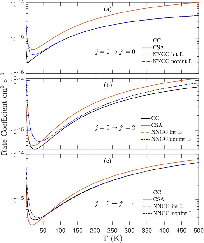
Figure 10: State-to-state rate coefficients as functions of the temperature calculated for initial state $v=1,j=0$ and final states $v^{\prime}=0,j^{\prime}=0$ (a), $v^{\prime}=0,j^{\prime}=2$ (b), and $v^{\prime}=0,j^{\prime}=4$ (c), with the ICSs shown in Fig. 6 (a), (b), and (c).

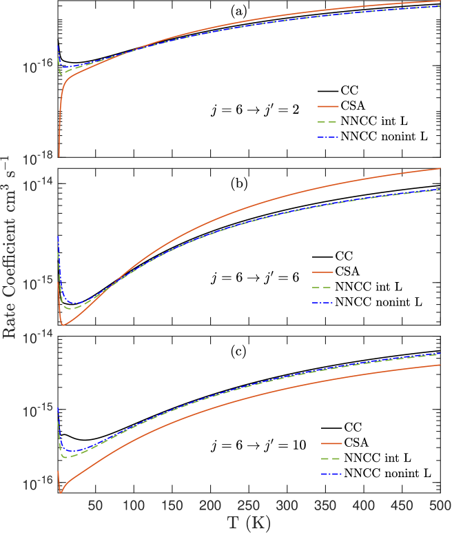
Figure 11: State-to-state rate coefficients as functions of the temperature calculated for initial state $v=1,j=6$ and final states $v^{\prime}=0,j^{\prime}=2$ (a), $v^{\prime}=0,j^{\prime}=6$ (b), and $v^{\prime}=0,j^{\prime}=10$ (c), with the ICSs shown in Fig. 7 (a), (b), and (c).

So far we discussed the ICSs from different methods as functions of the collision energy, but in astrophysical modeling one needs collisional rate coefficients as functions of the temperature. Figures 10 and 11 show state-to-state rate coefficients calculated from the ICSs displayed in Figs. 6 and 7. It is clear that the conclusions discussed above for the ICSs apply also to the rate coefficients. That is, the NNCC method is clearly superior to the CSA method in reproducing the full CC results.

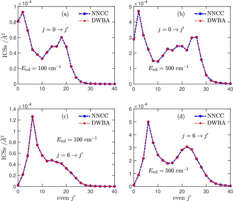
Figure 12: Product ($v^{\prime}=0,j^{\prime}$) distributions from the NNCC method with non-integer $L$ values, compared with results from MC-DWBA applied to this method. Panels (a) and (b) are for initial state $v=1,j=0$ at collision energies $E=100$ and 500 cm^-1, respectively, panels (c) and (d) for initial state $v=1,j=6$ at the same collision energies.

Finally, Fig. 12 demonstrates that state-to-state ICSs for rovibrationally inelastic collisions from the NNCC method are accurately reproduced by combining this method with MC-DWBA. This is very useful, as it shows that MC-DWBA cannot only be applied to the full CC method, as in Ref. selim:21 , but also to more approximate and less expensive methods.

Another issue to be discussed is: how much more efficient are the CSA and NNCC methods than the full CC method, both in terms of computer memory and CPU time. We checked this in calculations with a basis of CO₂ rotational functions up to $j=100$ for $v=0$ and 1, and total angular momentum $J=100$. As initial state we took $v=1,j=6$, so in the CSA calculations we needed to solve seven sets of coupled-channel equations for $\tilde{\Omega}$ in the symmetry-adapted basis ranging from 0 to 6. The NNCC method includes blocks with $\Omega$ and $\Omega\pm 1$ and we had to make calculations for $\tilde{\Omega}$ = [0,1,2], [1,2,3], [2,3,4], [3,4,5], [4,5,6], and [5,6,7]. The number of channels in the CC calculations was 5202, in CSA it was 100, and in NNCC it was 290. The size of the matrices involved in solving the coupled-channel problem depends quadratically on the number of channels, so it is clear that the CSA and NNCC methods allow one to handle much larger problems than the full CC method. Even more significant is the CPU time for the propagation, which depends roughly on the third power of the number of channels. Our renormalized Numerov propagation involved 501 steps and took 6633 CPU seconds for the CC method, 0.40 seconds for CSA, and 4.15 seconds for NNCC on a single Intel Xeon Platinum 8268 processor. So even with the more advanced NNCC approximation the savings in CPU time relative to full CC calculations is substantial. We note here that the actual gain in CPU time and matrix size in CSA and NNCC with respect to full CC calculations depends on the characteristics of the channel basis. In our calculations of the cross sections in rovibrationally inelastic CO₂-He collisions, we had to use a channel basis with large maximum values of the monomer rotational angular momentum $j$ and of the total angular momentum $J$.

In Ref. selim:21 we explained that the MC-DWBA method applied in full CC calculations reduces the CPU time by about a factor of 3. Here we find that also when combined with the NNCC method MC-DWBA leads to a further decrease of CPU time by a factor of 3.

IV Conclusions

The advanced models currently being developed by astronomers bosman:17 ; bosman:19 and the availability of data from the James Webb space telescope (JWST) in the near future require the knowledge of rovibrational state-to-state collisional rate coefficients. These rate coefficients can be obtained from coupled-channel (CC) scattering calculations, but these are very demanding. Here we presented more efficient methods based on the coupled-states approximation (CSA) in which one neglects the off-diagonal Coriolis coupling in the scattering Hamiltonian in body-fixed coordinates. This makes $\Omega$, the projection of the total angular momentum $J$ on the intermolecular axis, a good quantum number, so that scattering calculations can be performed independently for each $\Omega$. In addition to CSA, we investigated a method called NNCC (nearest-neighbor Coriolis coupling) yang:18 that includes Coriolis coupling to first order by simultaneously including basis functions with $\Omega$ and $\Omega\pm 1$. The NNCC method is more expensive than the CSA method, but still much more efficient than full CC calculations. We tested three versions of the CSA method and two versions of the NNCC method. The cross sections and rate coefficients from the two NNCC methods are similar, and substantially better than all CSA results.

All of this is illustrated by showing state-to-state cross sections and rate coefficients of rovibrational transitions induced in CO₂ by collisions with He atoms. Results from the CSA and NNCC methods are compared in detail with those from full CC calculations. In a recent paper selim:21 we have shown that the application of the multi-channel distorted-wave Born approximation (MC-DWBA) in CC calculations reduces the required CPU time by a factor of 3. Here we show that a further increase of effiency by about the same factor can be obtained by applying MC-DWBA to the NNCC method, with practically no loss of accuracy.

Finally we note that rovibrational transitions in CO₂ are probably more strongly induced by collisions with H₂ than by collisions with He, for several reasons. First, CO₂-H₂ interactions are stronger than CO₂-He interactions because H₂ is more polarizable than He and it has a quadrupole moment. Secondly, as was recently shown for rovibrationally inelastic H₂O-H₂ collisions wiesenfeld:21 , such transitions may be enhanced by simultaneous rotational excitation of H₂. The channel basis needed in CO₂-H₂ scattering calculations will be even larger than the bases we used for CO₂-He and the efficient methods to compute rovibrationally inelastic collision cross sections and rate coefficients presented here will be very advantageous.

Data availability

The data that supports the findings of this study are available within the article.

References

- (1) K. M. Pontoppidan, G. A. Blake, E. F. van Dishoeck, A. Smette, M. J. Ireland, and J. Brown, Astrophys. J. 684, 1323 (2008).
- (2) A. M. Mandell, J. Bast, E. F. van Dishoeck, G. A. Blake, C. Salyk, M. J. Mumma, and G. Villanueva, Astrophys. J. 747, 92 (2012).
- (3) S. Bruderer, D. Harsono, and E. F. van Dishoeck, Astron. Astrophys. 575, A94 (2015).
- (4) A. D. Bosman, S. Bruderer, and E. F. van Dishoeck, Astron. Astrophys. 601, A36 (2017).
- (5) A. D. Bosman, Uncovering the ingredients for planet formation, PhD thesis, Leiden University, 2019.
- (6) K. I. Öberg, A. C. A. Boogert, K. M. Pontoppidan, S. van den Broek, E. F. van Dishoeck, S. Bottinelli, G. A. Blake, and N. J. Evans, Astrophys. J 740, 109 (2011).
- (7) A. G. Palluet, F. Thibault, and F. Lique, J. Chem. Phys. 156, 104303 (2022).
- (8) D. C. Clary, J. Chem. Phys. 75, 209 (1981).
- (9) D. C. Clary, Chem. Phys. 65, 247 (1982).
- (10) A. J. Banks and D. C. Clary, J. Chem. Phys. 86, 802 (1987).
- (11) C. T. Wickham-Jones, C. J. S. M. Simpson, and D. C. Clary, Chem. Phys. 117, 9 (1987).
- (12) T. Selim, A. Christianen, A. van der Avoird, and G. C. Groenenboom, J. Chem. Phys. 155, 034105 (2021).
- (13) A. van der Avoird, P. E. S. Wormer, and R. Moszynski, Chem. Rev. 94, 1931 (1994).
- (14) A. M. Arthurs and A. Dalgarno, Proc. R. Soc. London, Ser. A 256, 540 (1960).
- (15) B. R. Johnson, J. Chem. Phys. 69, 4678 (1978).
- (16) B. R. Johnson, NRCC Proceedings 5, 86 (1979).
- (17) M. Abramowitz and I. A. Stegun, Handbook of Mathematical Functions, National Bureau of Standards, Washington, D.C., 1964.
- (18) P. McGuire and D. J. Kouri, J. Chem. Phys. 60, 2488 (1974).
- (19) D. Yang, X. Hu, D. H. Zhang, and D. Xie, J. Chem. Phys. 148, 084101 (2018).
- (20) D. Skouteris, J. F. Castillo, and D. E. Manolopoulos, Comput. Phys. Commun. 133, 128 (2000).
- (21) E. P. Wigner, Phys. Rev. 73, 1002 (1948).
- (22) L. Wiesenfeld, J. Chem. Phys. 155, 071104 (2021).