Towards Understanding Graph Neural Networks:
An Algorithm Unrolling Perspective

Abstract

The graph neural network (GNN) has demonstrated its superior performance in various applications. The working mechanism behind it, however, remains mysterious. GNN models are designed to learn effective representations for graph-structured data, which intrinsically coincides with the principle of graph signal denoising (GSD). Algorithm unrolling, a “learning to optimize” technique, has gained increasing attention due to its prospects in building efficient and interpretable neural network architectures. In this paper, we introduce a class of unrolled networks built based on truncated optimization algorithms (e.g., gradient descent and proximal gradient descent) for GSD problems. They are shown to be tightly connected to many popular GNN models in that the forward propagations in these GNNs are in fact unrolled networks serving specific GSDs. Besides, the training process of a GNN model can be seen as solving a bilevel optimization problem with a GSD problem at the lower level. Such a connection brings a fresh view of GNNs, as we could try to understand their practical capabilities from their GSD counterparts, and it can also motivate designing new GNN models. Based on the algorithm unrolling perspective, an expressive model named UGDGNN, i.e., unrolled gradient descent GNN, is further proposed which inherits appealing theoretical properties. Extensive numerical simulations on seven benchmark datasets demonstrate that UGDGNN can achieve superior or competitive performance over the state-of-the-art models.

1 Introduction

As the graph-structured data becomes largely available in various applications [40, 53], analyses of high-dimensional data over graph and/or other irregular domains have recently drawn unprecedented attention from researchers in machine learning, signal processing, statistics, etc. Among many other approaches, the graph neural network (GNN) models [29, 72, 59, 70, 58] have become prevalent due to their convincing performance and have been widely used in recommender system [66], computer vision [47], mathematical optimization [4], and many other application fields [19, 67, 45, 57].

The GNN models are deep learning-based methods operating on the graph domain that are designed to extract useful high-dimensional representations from the raw input graph-structured data (or signals). Typically, a GNN is a neural network consists of consecutive propagation layers, each of which contains two steps, namely, the feature aggregation (FA) step (i.e., each node aggregates the features from its neighborhood) and the feature transformation (FT) step (i.e., the aggregated features are further transformed at each node) [21, 54, 68, 44]. It has been shown that a single FA step in graph convolutional network (GCN) [29] and simple graph convolution network (SGC) [56] can be seen as a special form of Laplacian smoothing [33, 23, 62]. Inspired by this result, some recent works aim at interpreting one FA step in some other GNNs with a Laplacian regularized optimization problem [74, 38]. However, all the existing analyses in the literature isolate the consecutive propagation layers of the GNN models and further merely focus on the FA step in one propagation layer. Hence, their results neglect not only the accompanying indispensable FT step in each layer but also the propagation nature between consecutive layers of GNNs. Failing to capture the GNN structures as a whole, such over-simplified analyses will inevitably lead to conclusions that are discrepant with the practical capabilities of GNNs [61, 73, 11]. Then a natural research question arises: Can we interpret the existing GNN models with multiple consecutive feature propagation layers in a holistic way?

This paper gives an affirmative answer to the above question from the perspective of algorithm unrolling [20]. Algorithm unrolling falls into the “learning to optimize” paradigm and is regarded to be a promising technique for efficient and interpretable neural network architecture design [20, 39, 6]. The idea of algorithm unrolling is to transform a truncated iterative algorithm (i.e., an algorithm with finite steps) into a neural network, called an “unrolled network,” by converting some parameters of the updating steps in the original iterative algorithms into learnable weights in the unrolled network.

In this paper, we initiate our discussion with a bilevel optimization problem [13], where the upper-level problem is to minimize a task-tailored supervised loss and in the lower level is a graph signal denoising (GSD) optimization problem [50, 52]. The GSD problems aim at recovering the denoised graph signals from certain noisy input graph signals, which conceptually share the same spirit as the GNN models, i.e., learning effective graph representations from the raw input graph features. In practice, formulations for GSD problems are diverse due to the varying intended denoising targets. Analogously, different GNN models exhibit different model structures and/or parameters. After that, we present two unrolled networks for solving the GSD problems, namely, unrolled gradient descent (GD) network and unrolled proximal gradient descent (ProxGD) network. It turns out that a class of widely used GNN models are specializations or variants of these two unrolled networks. Therefore, training a GNN via backpropagation can be regarded as solving a bilevel optimization problem. On this basis, some novel inherent characteristics of the existing GNN models can further be revealed from their GSD counterparts and new GNN models with desired properties can also be developed.

To make it clear, main contributions of this paper are summarized in the following.

• We present a unified algorithm unrolling perspective on GNNs, based on which we demonstrate that many existing GNN models can be naturally interpreted as either an unrolled GD network or an unrolled ProxGD network for solving certain GSD problems. With this, for the first time, we accomplish a holistic understanding of GNNs as solving GSD problems.

• The fresh algorithm unrolling perspective on GNNs implies that training a GNN model can be naturally seen as solving a bilevel optimization problem with supervised loss at the upper level and a GSD problem at the lower level, which is tackled via an interpretable unrolled neural network corresponding to the consecutive propagation layers in the GNN model.

• Based on the algorithm unrolling perspective, a novel GNN with appealing expressive power is proposed leveraging the unrolled GD network for GSDs, hence named as UGDGNN.

• Extensive experimental results on seven benchmark datasets verify the effectiveness of UGDGNN and some of the theoretical conjectures made along this paper. The applaudable empirical results signify the promising prospects of interpreting existing GNNs as well as designing new GNN architectures from the algorithm unrolling perspective.

Due to space limit, proofs for the main results and further discussions are all deferred to the Appendix.

2 Preliminaries

Notations. An undirected unweighted graph with self-loops is denoted as $\mathcal{G}=(\mathcal{V},\mathcal{E})$, where $\mathcal{V}=\{1,\ldots,|\mathcal{V}|\}$ and $\mathcal{E}$ are the node set and the edge set, respectively. Suppose the $n$-th ($n\in\mathcal{V}$) node is associated with a feature vector $\mathbf{x}_{n}$, $\mathbf{X}=[\mathbf{x}_{1},\ldots,\mathbf{x}_{|\mathcal{V}|}]^{T}$ represents the overall graph feature matrix. Each column of $\mathbf{X}$ is a one-dimensional graph signal and $\mathbf{X}$ is essentially a multi-dimensional graph signal. The graph adjacency structure can be encoded by the adjacency matrix $\mathbf{A}\in\mathbb{R}^{|\mathcal{V}|\times|\mathcal{V}|}$. The degree matrix $\mathbf{D}\in\mathbb{R}^{|\mathcal{V}|\times|\mathcal{V}|}$ is defined by $\mathbf{D}=\mathsf{diag}(\mathbf{A}\mathbf{1})$. The Laplacian matrix is $\mathbf{L}=\mathbf{D}-\mathbf{A}$ and we also have $\mathbf{L}=\mathbf{B}^{T}\mathbf{B}$ with $\mathbf{B}$ being an oriented edge-node incident matrix (the orientation can be arbitrary). In the GNN literature, the symmetric normalized adjacency matrix $\hat{\mathbf{A}}=\mathbf{D}^{-\frac{1}{2}}\mathbf{A}\mathbf{D}^{-\frac{1}{2}}$ and the symmetric normalized Laplacian matrix $\hat{\mathbf{L}}=\mathbf{I}-\hat{\mathbf{A}}=\mathbf{D}^{-\frac{1}{2}}\mathbf{L}\mathbf{D}^{-\frac{1}{2}}=\hat{\mathbf{B}}^{T}\hat{\mathbf{B}}$ with $\hat{\mathbf{B}}=\mathbf{B}\mathbf{D}^{-\frac{1}{2}}$ are more commonly used. With a slight abuse of notation, in the following sections we will adopt the unhatted notations to represent the normalized graph matrices for notational simplicity.

2.1 Graph Signal Denoising Problems

As a fundamental problem in signal processing over graphs, GSD aims to recover a denoised graph signal $\mathbf{H}$ from the noisy graph signal $\mathbf{X}$ [50, 27, 52]. Under the smoothness assumption (i.e., signals in adjacent nodes are close in value), a vanilla GSD optimization problem is given as follows:

$$\underset{\mathbf{H}\in\mathcal{H}}{\mathrm{min}} \alpha\left\|\mathbf{H}-\mathbf{X}\right\|_{F}^{2}+\beta\mathrm{tr}\bigl{(}\mathbf{H}^{T}\mathbf{L}\mathbf{H}\bigr{)},$$ (1)

where $\mathcal{H}$ represents some possible constraints on $\mathbf{H}$, and $\alpha$, $\beta\geq 0$ adjust the relative importance of the two terms in the objective. To be specific, the first term is the signal fidelity term that guides $\mathbf{H}$ to be as close to $\mathbf{X}$ as possible, and the second term is the signal smoothing term (actually a Laplacian smoothing term, a.k.a. Laplacian regularization) that promotes smoothness of the denoised graph signal $\mathbf{H}$ (note that since $\mathbf{L}=\mathbf{B}^{T}\mathbf{B}$ we have $\mathrm{tr}(\mathbf{H}^{T}\mathbf{L}\mathbf{H})\negthinspace=\negthinspace||\mathbf{B}\mathbf{H}||_{F}^{2}$). As in the widely studied generalized regression and generalized low-rank approximation problems [51], we can always replace the Frobenius norms in (1) with their weighted alternatives defined by $||\mathbf{M}||_{\mathbf{T}}^{2}\coloneqq\mathrm{tr}(\mathbf{M}\mathbf{T}\mathbf{M}^{T})$ where $\mathbf{T}$ is symmetric. Then, we obtain the following general GSD problem:

$$\underset{\mathbf{H}}{\mathrm{min}} \underset{\eqqcolon L\left(\mathbf{H};\boldsymbol{\Theta},\mathbf{X},\mathbf{B}\right)}{\underbrace{\alpha\bigl{\|}\mathbf{H}-\mathbf{X}\bigr{\|}_{\mathbf{T}_{\alpha}}^{2}+\beta\bigl{\|}\mathbf{B}\mathbf{H}\bigr{\|}_{\mathbf{T}_{\beta}}^{2}+r(\mathbf{H})}},$$ (2)

where $\mathbf{T}_{\alpha}$ and $\mathbf{T}_{\beta}$ generally represent certain prior information on the target of GSD (For instance, $\mathbf{T}_{\alpha}$ could be chosen as the inverse covariance matrix of the noise, and $\mathbf{T}_{\beta}$ can be used to enforce different levels of smoothness on different nodes. Specially, a positive $t_{\beta,ii}$ promotes smoothness while a negative $t_{\beta,ii}$ promotes non-smoothness between nodes connected by the $i$-th edge, which facilitates learning over both homogeneous and heterogeneous graphs.) and $r(\mathbf{H})$ is a regularization term which can be used to impose constraints or other penalizations. We have denoted the objective function as $L\left(\mathbf{H};\boldsymbol{\Theta},\mathbf{X},\mathbf{B}\right)$ where $\boldsymbol{\Theta}$ collects all the model parameters including $\alpha$, $\beta$, $\mathbf{T}_{\alpha}$, and $\mathbf{T}_{\beta}$. In addition, problem (2) will degenerate to the vanilla GSD problem (1) when $\mathbf{T}_{\alpha}=\mathbf{T}_{\beta}=\mathbf{I}$ and $r(\mathbf{H})=I_{\mathcal{H}}(\mathbf{H})$, where $I(\cdot)$ denotes the indicator function taking value 0 if $\mathbf{H}\in\mathcal{H}$ and $+\infty$ otherwise. Based on the GSD problems defined above, we can see the goals of GSD are intrinsically similar to those of GNN, i.e., extracting certain “useful information” from the noisy inputs.

2.2 Algorithm Unrolling

Algorithm unrolling, a.k.a. algorithm unfolding, is a “learning to optimize” paradigm for neural network architecture design, which “unrolls” a truncated classical iterative algorithm (i.e., an iterative algorithm only with finite iteration steps) into a neural network [20, 39, 6], named an “unrolled network.” To design an unrolled network, some of the parameters in one updating step from the original iterative algorithm will be translated to be the trainable weights in one network layer, and a finite number of layers are then concatenated together. Such a trained neural network will naturally carry out the interpretation of a “parameter-optimized iterative algorithm” [64]. Therefore, passing through an unrolled network with a finite number of layers amounts to execute an iterative algorithm for a finite number of steps, which brings interpretability to the neural network.

In constructing an unrolled network, a key procedure is to determine how to parameterize the underlying iterative algorithm (considerations may include which parameters are translated to be the learnable weights in the network, setting the parameters in different layers to be shared or independent, etc.). The algorithm unrolling scheme was first used to unroll the famous iterative soft-thresholding algorithm [20], i.e., proximal gradient, for sparse coding problems, where hyperparameters in the algorithm are chosen to be learnable and set to be shared over different layers, i.e., a recurrent structure. After that, some other works [22, 1, 8, 34] drop the recurrent structure scheme and untie the learnable weights; i.e., weights in different layers can be different and hence optimized independently. These models with untying parameters can enlarge the capacity of the unrolled networks [22]. Although research on the theoretical characterizations between these unrolled networks and their analytic iterative algorithm counterparts are still evolving [39, 6], interpreting popular neural network architectures from the algorithm unrolling perspective can always enrich the understanding of their capacities. For example, authors in [43] analyzed the properties of the convolutional neural networks by viewing them as unrolled networks. To the best of our knowledge, the relationship between algorithm unrolling and the existing GNN models remains unexplored.

3 A Unified Algorithm Unrolling Perspective on GNN Models

We launch our discussion on the “intimate correspondence” between GNN models and GSD optimization problems through investigating a bilevel optimization problem [13] defined as follows:

$$\underset{\boldsymbol{\theta}\in\varTheta,\bar{\mathbf{X}}}{\mathrm{min}} U\left(\mathbf{Y},p_{\mathsf{pos}}(\bar{\mathbf{X}})\right) \mathsf{(upper)}$$ (3)

$$\;\>\mathrm{s.t.} \bar{\mathbf{X}}\in\mathrm{arg}\min_{\mathbf{H}}L\Biggl{(}\mathbf{H};\boldsymbol{\Theta},\underset{\eqqcolon\mathbf{X}}{\underbrace{p_{\mathsf{pre}}\left(\tilde{\mathbf{X}}\right)}},\mathbf{B}\Biggr{)}, \mathsf{(lower)}$$

where the optimization variables are all the model parameters $\boldsymbol{\theta}\coloneqq\{\boldsymbol{\Theta},\text{prameters in }p_{\mathsf{pos}}\text{\text{ and }}p_{\mathsf{pre}}\}$ with $\varTheta$ denoting the parameter space and the output $\bar{\mathbf{X}}$ of the lower-level problem. The objective $U$ in the upper level represents the supervised loss for downstream tasks like clustering, classification, ranking, etc., with $\mathbf{Y}$ denoting the label matrix and $p_{\mathsf{pos}}(\bar{\mathbf{X}})$ representing some possible post-processing procedures for $\bar{\mathbf{X}}$. The lower-level problem is a GSD problem as defined in (2). Instead of denoising the raw input graph signal $\tilde{\mathbf{X}}$ directly, certain pre-processing operations may also be imposed before it is fed into the GSD problem, which is generally denoted by $p_{\mathsf{pre}}(\tilde{\mathbf{X}})$, whose output is defined as $\mathbf{X}$.

Example 1 (Semi-supervised node classification).

Consider a semi-supervised node classification problem, where we can only access labels of a subset of nodes, i.e., $\mathcal{V}^{\prime}\subset\mathcal{V}$. The target is to train a GNN model based on the raw node features of all nodes $\tilde{\mathbf{X}}$ and the node labels in the subset $\{\mathbf{y}_{i}\}_{i\in\mathcal{V}^{\prime}}$, and to expect it can generalize well on the unlabeled node set $\mathcal{V}\setminus\mathcal{V}^{\prime}$. In this case, we can choose $U$ as the cross-entropy loss function, $p_{\mathsf{pos}}$ as the $\mathrm{softmax}$ function, and $p_{\mathsf{pre}}$ as a multi-layer perceptron.

Generally speaking, solving the nested optimization problem (3) is challenging as it involves solving the upper- and lower-level problems simultaneously. If an analytical solution to the lower-level problem can be obtained and then substituted into the upper level, the bilevel problem will reduce to a single-level one, which could be easier to handle. In case that analytical solutions for the lower-level problem are not available (or expensive to compute), one can resort to an iterative algorithm (e.g., GD, ProxGD, Newton’s methods, etc.) to generate an approximate solution by conducting a finite number of iterations. To expand the capacity of an iterative algorithm, the algorithm unrolling technique can be used to construct an unrolled network. Given an initialization $\mathbf{H}^{(0)}$, passing it through an $K$-layer unrolled network imitates the behavior of executing an iterative algorithm for $K$ steps, generating the sequence $\{\mathbf{H}^{(k)}\}_{k=1}^{K}$. Under certain conditions, convergence of $\{\mathbf{H}^{(k)}\}_{k=1}^{K}$ to $\bar{\mathbf{X}}$ can be established [8]. With a slight abuse of notation, $\bar{\mathbf{X}}$ and $\mathbf{H}^{(K)}$ will be used interchangeably in discussing GNNs.

Specifically, applying the idea of algorithm unrolling to an iterative algorithm that solves the GSD optimization problem at the lower level of (3), an unrolled network for graph representation leaning will be obtained. Its parameters are to be learned through optimizing the loss at the upper level. In the following, we show that a class of widely used existing GNN models naturally emerge out of unrolled GD or unrolled ProxGD networks for solving GSD problems, based on which training these GNNs is equivalent to solving a bilevel optimization problem with certain GSDs at the lower level.

3.1 GNNs as Unrolled GD Networks for GSDs

It turns out that many popular GNN models can be seen as unrolled GD networks for GSDs. Denote the objective in (2) as $L(\mathbf{H})$ for brevity. The update in GD with properly chosen stepsize $\eta^{(k)}>0$ is

$$\mathbf{H}^{(k)}=\mathbf{H}^{(k-1)}-\eta^{(k)}\nabla L(\mathbf{H}^{(k-1)}).$$

With $r(\mathbf{H})=0$, the GSD objective $L(\mathbf{H})$ in (2) is smooth and the gradient of $L(\mathbf{H})$ is

$$\nabla L(\mathbf{H})=2\alpha\bigl{(}\mathbf{H}-\mathbf{X}\bigr{)}\mathbf{T}_{\alpha}+2\beta\mathbf{B}^{T}\mathbf{B}\mathbf{H}\mathbf{T}_{\beta},$$ (4)

and accordingly the GD step is given by

$$\mathbf{H}^{(k)}=\mathbf{H}^{(k-1)}\bigl{(}\mathbf{I}-2\eta^{(k)}\alpha\mathbf{T}_{\alpha}-2\eta^{(k)}\beta\mathbf{T}_{\beta}\bigr{)}+2\eta^{(k)}\beta\mathbf{A}\mathbf{H}^{(k-1)}\mathbf{T}_{\beta}+2\eta^{(k)}\alpha\mathbf{X}\mathbf{T}_{\alpha},$$

where we have used the relation $\mathbf{B}^{T}\mathbf{B}=\mathbf{I}-\mathbf{A}$. Following the algorithm unrolling paradigm, by letting the stepsize parameter $\eta^{(k)}$ and model parameters $\boldsymbol{\Theta}$ (i.e., $\alpha$, $\beta$, $\mathbf{T}_{\alpha}$, and $\mathbf{T}_{\beta}$) in the GSD problems to be learnable and concatenating $K$ unrolled GD layers together, a GNN model can be naturally constructed as an unrolled GD neural network.

Theorem 2.

A general $K$-layer GNN model can be obtained by unrolling $K$ GD steps for an unconstrained GSD problem (2) (i.e., $r(\mathbf{H})=0$), in which the $k$-th propagation layer is given by

$$\mathbf{H}^{(k)}=\mathbf{H}^{(k-1)}\bigl{(}\mathbf{I}-2\eta^{(k)}\alpha^{(k)}\mathbf{T}_{\alpha}^{(k)}-2\eta^{(k)}\beta^{(k)}\mathbf{T}_{\beta}^{(k)}\bigr{)}$$ (5)

$$\hskip 72.55461pt+2\eta^{(k)}\beta^{(k)}\mathbf{A}\mathbf{H}^{(k-1)}\mathbf{T}_{\beta}^{(k)}+2\eta^{(k)}\alpha^{(k)}\mathbf{X}\mathbf{T}_{\alpha}^{(k)},\ \text{for}\ k=1,\ldots,K,$$

where $\eta^{(k)}$, $\alpha^{(k)}$, $\beta^{(k)}$, $\mathbf{T}_{\alpha}^{(k)}$, and $\mathbf{T}_{\beta}^{(k)}$ are the learnable parameters in the $k$-th network layer.

In an unrolled GD layer (5), i.e., a propagation layer (including one FA step and one FT step) of a general GNN model, the parameters $\eta^{(k)}$, $\alpha^{(k)}$, and $\beta^{(k)}$ jointly control the strength of neighborhood aggregation, residual connection, and initial residual connection. Unlike the existing works [42, 74, 38] that only interpret the FA step in one propagation layer without taking the indispensable transformation weight matrices into account and hence may be myopic or hyperopic, our interpretation of a propagation layer as given in (5) can be easily extended to interpret the consecutive propagation nature of GNN models in a holistic manner. It should also be noted that although the unrolled GD layer in (5) seems to be very comprehensive, this neural network is actually a structured and interpretable model because it is unrolled based on GD for a prescribed GSD problem. It can be shown that existing GNNs can be seen as specializations or variants of this unrolled GD network.

In the following, we will elaborate four representative GNNs as unrolled GD networks for GSDs, that is, SGC [56], approximate personalized propagation of neural predictions (APPNP) [30], jumping knowledge networks (JKNet) [60], and generalized PageRank GNN (GPRGNN) [9]. Note that for all models, the specific parameterization schemes in unrolled networks are elaborated in the Appendix.

SGC. The SGC [56] performs a finite number of FA steps (i.e., recursively premultiplying $\mathbf{A}$ to the current feature) followed by a linear transformation. To be specific, a $K$-layer SGC is defined as

$$\bar{\mathbf{X}}=\mathbf{A}^{K}\mathbf{X}\mathbf{W},$$ (6)

where $\mathbf{W}$ is a learnable parameter. The relation between SGC and GSD is given in Proposition 3.

Proposition 3.

Passing through a $K$-layer SGC model is equivalent to solving a GSD problem (2) with $\alpha=0$ and $r(\mathbf{H})=\beta||\mathbf{H}||_{\mathbf{I}-\mathbf{T}_{\beta}}^{2}$ via a $K$-layer unrolled GD network.

In Proposition 3, we have assumed the learnable weight matrix $\mathbf{W}$ is induced from parameter $\boldsymbol{\Theta}$, while it actually can also be cast as a part of $p_{\mathsf{pre}}$ or $p_{\mathsf{pos}}$ (refer to Appendix for detailed discussions).

PPNP & APPNP. It has been discussed in [30] that as $K\rightarrow+\infty$, the aggregation scheme in SGC will lead to a limit point that has a similar expression as in PageRank [41]. Based on the relationship between SGC and PageRank, the PPNP model [30] was proposed based on personalized PageRank [41], whose propagation mechanism is

$$\bar{\mathbf{X}}=\gamma\bigl{(}\mathbf{I}-(1-\gamma)\mathbf{A}\bigr{)}^{-1}\mathbf{X},$$

where $\gamma$ is a given teleport probability. To avoid the computationally inefficient matrix inverse operation, an approximation of PPNP called APPNP [30] was proposed. A $K$-layer APPNP is

$$\bar{\mathbf{X}}=\mathbf{H}^{(K)},\ \ \ \mathbf{H}^{(k)}=\left(1-\gamma\right)\mathbf{A}\mathbf{H}^{(k-1)}+\gamma\mathbf{X},\ \text{for}\ k=1,\ldots,K.$$

The relation between PPNP & APPNP and GSD problems is summarized in the following proposition.

Proposition 4.

The PPNP model analytically solves the GSD problem (2) with $\beta=1-\alpha$, $\mathbf{T}_{\alpha}=\mathbf{T}_{\beta}=\mathbf{I}$, and $r(\mathbf{H})=0$, while a $K$ layer APPNP model solves it via a $K$-layer unrolled GD network. Moreover, the teleport probability $\gamma$ in PPNP & APPNP is equal to $\alpha$ in the underlying GSD problem.

Based on Proposition 4, a smaller $\gamma$ in APPNP & PPNP, i.e., a smaller $\alpha$ and hence a relatively larger $\beta$ in GSD, can enforce the graph signal to be smoother, corroborating the meaning of parameter $\gamma$.

JKNet. In SGC, the nodes in graph can only access information from a fixed-size neighborhood. To make each node adaptively leverage the information from its effective neighborhood size, the JKNet model [60] selectively combines the intermediate node representations from each layer into its output. The JKNet model permits general representation combination schemes, but for simplicity we consider the summation scheme here. A $K$-layer JKNet applies the following operation to the input $\mathbf{X}$:

$$\bar{\mathbf{X}}=\sum_{k=0}^{K}\mathbf{A}^{k}\mathbf{X}\mathbf{W}^{(k)},$$ (7)

where $\{\mathbf{W}^{(k)}\}_{k=1}^{K}$ are the learnable weights. The relation between JKNet and GSD is given below.

Proposition 5.

By concatenating $K$ unrolled GD layers for solving a GSD problem (2) with $\alpha=\beta$, $\mathbf{T}_{\alpha}=\mathbf{I}-\mathbf{T}_{\beta}$, and $r(\mathbf{H})=0$, we obtain a $K$-layer JKNet model.

GPRGNN. The generalized PageRank methods were first used in unsupervised graph clustering and demonstrated significant performance improvements over personalized PageRank methods [31, 32]. Inspired by that, the GPRGNN model [9] was brought up based on the generalized PageRank technique, which associates each step of feature aggregation with a learnable weight. A $K$-layer GPRGNN model is given as follows:

$$\bar{\mathbf{X}}=\sum_{k=0}^{K}\gamma^{(k)}\mathbf{A}^{k}\mathbf{X},$$ (8)

where $\{\gamma^{(k)}\}_{k=1}^{K}$ are learnable weights. The relation between GPRGNN and GSD is provided below.

Proposition 6.

A $K$-layer GPRGNN is equivalent to a $K$-layer unrolled GD network for solving a GSD problem (2) with $\beta=1-\alpha$, $\mathbf{T}_{\alpha}=\mathbf{T}_{\beta}=\mathbf{I}$, and $r(\mathbf{H})=0$.

Based on Proposition 4 and Proposition 6, we can conclude that APPNP and GPRGNN solve the same underlying GSD problem. Besides, GPRGNN can be seen as a generalization of APPNP by untying the shared parameter $\gamma$ in different unrolled GD layers. Therefore, GPRGNN is supposed to be more expressive and hence is expected to attain better performance than APPNP.

3.2 GNNs as Unrolled ProxGD Networks for GSDs

In the previous section, we have considered several GNNs only with linear FT steps. However, there are many GNN models that apply nonlinear FT steps. Considering the fact that every standard activation function (e.g., $\mathrm{ReLU}$, $\mathrm{ELU}$, and leaky $\mathrm{ReLU}$) can be derived from a proximity operator [10], GNNs with nonlinear FTs can be naturally interpreted as unrolled ProxGD networks for GSDs.

Table 1: The GSD objectives for different GNN models from the algorithm unrolling perspective.

Models	$K$-layer GNN Models	GSD Objectives
SGC	$\bar{\mathbf{X}}=\mathbf{A}^{K}\mathbf{X}\mathbf{W}$	$\bigl{\|}\mathbf{B}\mathbf{H}\bigr{\|}_{\mathbf{T}_{\beta}}^{2}+\bigl{\|}\mathbf{H}\bigr{\|}_{\mathbf{I}-\mathbf{T}_{\beta}}^{2}$
PPNP	$\bar{\mathbf{X}}=\gamma\bigl{(}\mathbf{I}-(1-\gamma)\mathbf{A}\bigr{)}^{-1}\mathbf{X}$	$\alpha\bigl{\|}\mathbf{H}-\mathbf{X}\bigr{\|}_{F}^{2}+(1-\alpha)\bigl{\|}\mathbf{B}\mathbf{H}\bigr{\|}_{F}^{2}$
APPNP	$\bar{\mathbf{X}}=\mathbf{H}^{(K)},\ \mathbf{H}^{(k)}=(1-\gamma)\mathbf{A}\mathbf{H}^{(k-1)}+\gamma\mathbf{X},\ \ k=1,\ldots,K$
JKNet	$\bar{\mathbf{X}}=\sum_{k=0}^{K}\mathbf{A}^{k}\mathbf{X}\mathbf{W}^{(k)}$	$\bigl{\|}\mathbf{H}-\mathbf{X}\bigr{\|}_{\mathbf{T}_{\alpha}}^{2}+\bigl{\|}\mathbf{B}\mathbf{H}\bigr{\|}_{\mathbf{I}-\mathbf{T}_{\alpha}}^{2}$
GPRGNN	$\bar{\mathbf{X}}=\sum_{k=0}^{K}\gamma^{(k)}\mathbf{A}^{k}\mathbf{X}$	$\alpha\bigl{\|}\mathbf{H}-\mathbf{X}\bigr{\|}_{F}^{2}+(1-\alpha)\bigl{\|}\mathbf{B}\mathbf{H}\bigr{\|}_{F}^{2}$
GCN	$\bar{\mathbf{X}}=\mathbf{H}^{(K)},\ \mathbf{H}^{(k)}=\mathrm{ReLU}\left(\mathbf{A}\mathbf{H}^{(k-1)}\mathbf{W}^{(k)}\right),\ \ k=1,\ldots,K$	$\bigl{\|}\mathbf{B}\mathbf{H}\bigr{\|}_{\mathbf{T}_{\beta}}^{2}+\bigl{\|}\mathbf{H}\bigr{\|}_{\mathbf{I}-\mathbf{T}_{\beta}}^{2}+I_{\{h_{ij}\geq 0,\ \forall i,j\}}(\mathbf{H})$
GCNII	$\bar{\mathbf{X}}=\mathbf{H}^{(K)},\ \mathbf{H}^{(k)}=\mathrm{ReLU}\Bigl{(}\bigl{(}\zeta\mathbf{A}\mathbf{H}^{(k-1)}+(1-\zeta)\mathbf{X}\bigr{)}$	$\left(1-\beta\right)\bigl{\|}\mathbf{H}-\mathbf{X}\bigr{\|}_{\mathbf{T}_{\beta}}^{2}+\beta\bigl{\|}\mathbf{B}\mathbf{H}\bigr{\|}_{\mathbf{T}_{\beta}}^{2}$
	$\hskip 85.35826pt\times\bigl{(}\xi\mathbf{W}^{(k)}+(1-\xi)\mathbf{I}\bigr{)}\Bigr{)},\ \ k=1,\ldots,K$	$\hskip 44.10185pt+\bigl{\|}\mathbf{H}\bigr{\|}_{\mathbf{I}-\mathbf{T}_{\beta}}^{2}+I_{\{h_{ij}\geq 0,\ \forall i,j\}}(\mathbf{H})$
AirGNN	$\bar{\mathbf{X}}=\mathbf{H}^{(K)},\ \mathbf{h}_{i}^{(k)}=\mathrm{ReLU}\Bigl{(}1-\frac{1-\gamma}{2\gamma||\mathbf{A}\mathbf{h}_{i}^{(k-1)}-\mathbf{x}_{i}||_{2}}\Bigr{)}$	$\beta\bigl{\|}\mathbf{B}\mathbf{H}\bigr{\|}_{F}^{2}+(1-\beta)\bigl{\|}\mathbf{H}-\mathbf{X}\bigr{\|}_{2,1}$
	$\hskip 59.75095pt\times\bigl{(}\mathbf{A}\mathbf{h}_{i}^{(k-1)}-\mathbf{x}_{i}\bigr{)}+\mathbf{x}_{i},\ i\in\mathcal{V},\ k=1,\ldots,K$
UGDGNN	$\bar{\mathbf{X}}=\sum_{k=0}^{K}\gamma^{(k)}\mathbf{A}^{k}\mathbf{X}\bigl{(}\zeta^{(k)}\mathbf{I}+\xi^{(k)}\mathbf{W}^{(k)}\bigr{)}$	$\alpha\bigl{\|}\mathbf{H}-\mathbf{X}\bigr{\|}_{\mathbf{T}_{\alpha}}^{2}+\beta\bigl{\|}\mathbf{B}\mathbf{H}\bigr{\|}_{\mathbf{T}_{\beta}}^{2}$

Consider Problem (2) with $r(\mathbf{H})=I_{\mathcal{H}}(\mathbf{H})$, we can apply the ProxGD algorithm for problem resolution and the $k$-th update step in ProxGD with properly chosen stepsize $\eta^{(k)}>0$ are given as

$$\mathbf{H}^{(k)} =\mathrm{prox}_{I}\bigl{(}\mathbf{H}^{(k-1)}-\eta^{(k)}\nabla\tilde{L}(\mathbf{H}^{(k-1)})\bigr{)},$$

where we use $\tilde{L}$ to denote the smooth part in $L$. By applying the algorithm unrolling idea to the ProxGD algorithm, we have the following result.

Theorem 7.

By unrolling $K$ ProxGD steps for a constrained GSD problem (2), we obtain a general $K$-layer GNN model with the $k$-th ($k=1,\ldots,K$) propagation layer defined as follows:

$$\mathbf{H}^{(k)} =\mathrm{prox}_{I}\bigl{(}\mathbf{H}^{(k-1)}\bigl{(}\mathbf{I}-2\eta^{(k)}\alpha^{(k)}\mathbf{T}_{\alpha}^{(k)}-2\eta^{(k)}\beta^{(k)}\mathbf{T}_{\beta}^{(k)}\bigr{)}$$ (9)

$$\hskip 72.55461pt+2\eta^{(k)}\beta^{(k)}\mathbf{A}\mathbf{H}^{(k-1)}\mathbf{T}_{\beta}^{(k)}+2\eta^{(k)}\alpha^{(k)}\mathbf{X}\mathbf{T}_{\alpha}^{(k)}\bigr{)},\ \text{for}\ k=1,\ldots,K,$$

where $\eta^{(k)}$, $\alpha^{(k)}$, $\beta^{(k)}$, $\mathbf{T}_{\alpha}^{(k)}$, and $\mathbf{T}_{\beta}^{(k)}$ are the learnable parameters in the $k$-th network layer.

Specifically, suppose we have the prior information that the graph signals of interest are non-negative, i.e., a non-negative GSD problem, we can set a constraint as $\mathcal{H}=\{h_{ij}\geq 0,\ \forall i,j\}$. Due to the fact that $\mathrm{prox}_{I(\{x\geq 0\})}(x)=\mathrm{ReLU}(x)$ [10], the activation function $\mathrm{ReLU}$ in a class of GNNs could be interpreted as unrolled ProxGD networks for non-negative GSDs. Similar to unrolled GD network, this model is highly structured and encompasses some existing GNN models. In the following, three representative GNNs that perform nonlinear FT steps are showcased, namely, GCN [29], GCN with initial residual and identity mapping (GCNII) [5], and GNN with adaptive residual (AirGNN) [36].

GCN. Although appearing earlier than SGC in the literature, the GCN model [29] can be regarded as a nonlinear extension of SGC by adding the nonlinear activation functions $\mathrm{ReLU}$ between consecutive propagation layers. The propagation mechanism of a $K$-layer GCN is

$$\bar{\mathbf{X}}=\mathbf{H}^{(K)},\ \ \ \mathbf{H}^{(k)}=\mathrm{ReLU}\bigl{(}\mathbf{A}\mathbf{H}^{(k-1)}\mathbf{W}^{(k)}\bigr{)},\ \text{for}\ k=1,\ldots,K,$$ (10)

where $\{\mathbf{W}^{(k)}\}_{k=1}^{K}$ are the weight matrices. The relation between GCN and GSD is illustrated below.

Proposition 8.

A $K$-layer GCN model is equivalent to a $K$-layer unrolled ProxGD network for solving a GSD problem (2) with $\alpha=0$ and $r(\mathbf{H})=\beta||\mathbf{H}||_{\mathbf{I}-\mathbf{T}_{\beta}}^{2}+I_{\{h_{ij}\geq 0,\ \forall i,j\}}(\mathbf{H})$.

Based on Proposition 8, we can conclude that the GCN model, owing to regularizer $r(\mathbf{H})$, does not merely perform the target of global smoothing, which is also supported by some recent works suggesting that oversmoothing does not necessarily happen in deep GCN models [61, 73, 11].

GCNII. The GCN model could suffer from a severe performance degradation as it becomes deeper. To resolve that performance degeneration issue, the GCNII model [5] was proposed with two simple yet effective techniques, namely, initial residual and identity mapping. A $K$-layer GCNII performs

$$\bar{\mathbf{X}}=\mathbf{H}^{(K)},\ \ \ \mathbf{H}^{(k)}=\mathrm{ReLU}\Bigl{(}\bigl{(}\zeta\mathbf{A}\mathbf{H}^{(k-1)}+(1-\zeta)\mathbf{X}\bigr{)}\bigl{(}\xi\mathbf{W}^{(k)}+(1-\xi)\mathbf{I}\bigr{)}\Bigr{)},\ \text{for}\ k=1,\ldots,K,$$

where $\zeta$ and $\xi$ are two prespecified parameters and $\mathbf{W}^{(k)}$ is a learnable matrix in the $k$-th layer. The relation between the GCNII model and GSD problem is demonstrated in the following proposition.

Proposition 9.

By concatenating $K$ unrolled ProxGD layers for a GSD problem (2) with $\beta=1-\alpha$, $\mathbf{T}_{\alpha}=\mathbf{T}_{\beta}$, and $r(\mathbf{H})=\left\|\mathbf{H}\right\|_{\mathbf{I}-\mathbf{T}_{\beta}}^{2}\negthinspace+I_{\{h_{ij}\geq 0,\ \forall i,j\}}(\mathbf{H})$, we obtain a $K$-layer GCNII model.

Based on the results in Proposition 8 and Proposition 9 , we find that the underlying GSD objective for GCNII has an additional signal fidelity term compared with that for GCN. This could be used to support the empirical evidence from many studies that the GCNII model is able to effectively relieve the performance degradation problem encountered in deep GCNs [5, 7].

AirGNN. Besides inducing nonlinearity to GNNs through imposing certain constraints $\mathcal{H}$ like the non-negativity constraint, nonlinear FT steps can also be derived through other ways. To make an example, we introduce the AirGNN model [36], which applies adaptive residual connections for different nodes. A $K$-layer AirGNN is given as follows:

$$\bar{\mathbf{X}} =\mathbf{H}^{(K)},\ \ \mathbf{h}_{i}^{(k)}=\mathrm{ReLU}\Bigl{(}1-\frac{1-\gamma}{2\gamma||[\mathbf{A}\mathbf{H}^{(k-1)}]_{i}-\mathbf{x}_{i}||_{2}}\Bigr{)}\bigl{(}[\mathbf{A}\mathbf{H}^{(k-1)}]_{i}-\mathbf{x}_{i}\bigr{)}+\mathbf{x}_{i},$$

$$\hskip 284.52756pt\ \text{for}\ i\in\mathcal{V},\ k=1,\ldots,K,$$

where $\mathbf{h}_{i}^{(k)}$ and $[\mathbf{A}\mathbf{H}^{(k-1)}]_{i}$ denote the $i$-th row of $\mathbf{H}^{(k)}$ and $\mathbf{A}\mathbf{H}^{(k-1)}$ respectively and $\gamma$ is a prespecified constant. The relation between AirGNN and GSD is illustrated in the following proposition.

Proposition 10.

A $K$-layer AirGNN model is equivalent to a $K$-layer unrolled ProxGD network for solving a GSD problem (2) with $\alpha=0$, $\mathbf{T}_{\alpha}=\mathbf{T}_{\beta}=\mathbf{I}$, and $r(\mathbf{H})=(1-\beta)||\mathbf{H}-\mathbf{X}||_{2,1}$.

The $||\mathbf{M}||_{2,1}$ denotes the $\ell_{2,1}$-norm of $\mathbf{M}$, defined as $||\mathbf{M}||_{2,1}=\sum_{i}||\mathbf{m}_{i}||_{2}$ with $\mathbf{m}_{i}$ the $i$-th row of $\mathbf{M}$. It is generally acknowledged that the $\ell_{1}$-norm is a robust loss function (corresponding to a Laplacian distribution prior) in comparison with the $\ell_{2}$-norm [25]. Therefore, the robustness of AirGNN against abnormal node features can be readily established by investigating its corresponding GSD problem.

So far, we have established the exact equivalence between a class of popular GNN models with the unrolled GD/ProxGD networks for GSD problems. We summarize all these connections in Table 1.

4 Proposed Model

For a GSD problem, if there is no prior knowledge on the signal, like to be non-negative, imposing constraints may restrict the design space and affect the solution quality. Besides, some recent works have empirically demonstrated that the nonlinearities are the main factor for performance degradations in deep GNNs, which hinders GNNs from learning node representations from large receptive fields [35, 73]. Moreover, some studies have theoretically shown that the nonlinearity in the propagation layers will hurt the generalization ability of GNNs [11]. Therefore, in this section, based on the GSD problem in (2), we propose to build a GNN via the unrolled GD layers.

In existing GNNs interpreted as unrolled GD networks, e.g., SGC, APPNP, JKNet, and GPRGNN, our analyses have shown that the choices of the model parameters $\eta^{(k)}$, $\alpha^{(k)}$, $\beta^{(k)}$, $\mathbf{T}_{\alpha}^{(k)}$, and $\mathbf{T}_{\beta}^{(k)}$, are mostly hand-crafted and heuristic. We conjecture that relieving such restrictions may help improving the model performance. However, directly concatenating the unrolled GD layers (5) involves too many cumbersome parameters which largely increases the model complexity. In the following, we propose a novel GNN model unrolled from GD to mitigate this problem, which is called UGDGNN.

Proposition 11.

Concatenating $K$ unrolled GD layers (5), we obtain the following UGDGNN model:

$$\bar{\mathbf{X}}=\sum_{k=0}^{K}\gamma^{(k)}\mathbf{A}^{k}\mathbf{X}\bigl{(}\zeta^{(k)}\mathbf{I}+\xi^{(k)}\mathbf{W}^{(k)}\bigr{)}.$$

For a $K$-layer GNN, the nodes are able to aggregate information from their $K$-th order neighborhood, which is to perform filtering in the vertex domain [50]. Since the UGDGNN model is derived from concatenating the general unrolled GD layers (5) without hand-crafted parameters, many existing GNN models (e.g., SGC, APPNP, JKNet, and GPRGNN) can be regarded as special cases of it, indicating the outstanding expressive power of UGDGNN in vertex domain (detailed discussions are given in Appendix). We further examine the expressive power of UGDGNN in the spectral domain.

Theorem 12.

A polynomial frequency filter of order $K$ is defined as $F_{K}(\mathbf{X})=\bigl{(}\sum_{k=0}^{K}\theta_{k}\mathbf{L}^{k}\bigr{)}\mathbf{X}$ with filtering coefficients $\theta_{k}$ for $k=0,\ldots,K$. A $K$-layer UGDGNN model can express any $F_{K}(\mathbf{X})$, i.e., a polynomial frequency filter of order $K$ with arbitrary coefficients.

Based on Theorem 12, UGDGNN is able to express a general polynomial graph filter and, hence, is capable of dealing with different graph signal patterns (e.g., graph signals with either high or low frequency components). By contrast, some existing GNNs mentioned in the previous sections only have limited spectral expressiveness, e.g., acting as a polynomial frequency filter with fixed coefficients (see details in Appendix). Therefore, UGDGNN exhibits favorable expressive powers in both the vertex domain and the spectral domain.

5 Experiments

Datasets. We conduct experiments on 7 datasets for semi-supervised node classification tasks that are widely used to evaluate GNNs in the literature, including three citation network datasets, i.e., Cora, Citeseer, and Pubmed [48], two co-authorship datasets, i.e., Coauthor CS and Coauthor Physics [49], a co-purchase dataset, i.e., Amazon Photo [49], and a citation network collected in open graph benchmark (OGB), i.e., the OGBN-ArXiv dataset [24].

Baselines. We compare the proposed UGDGNN with representative GNNs including GCN [29], SGC [56], APPNP [30], JKNet [60], GCNII [5], deep adaptive GNN (DAGNN) [35], GPRGNN [9].

Node classification results. The classification performance of different GNN models on all benchmark datasets are summarized in Table 2. Based on the results, we have the following observations.

Due to space limit, all the implementation details and hyperparameter settings are given in Appendix.

• UGDGNN achieves superior or competitive performance over the state-of-the-art GNNs on all the benchmark datasets. Such persuasive performance indicates the promising prospects of designing new GNNs from the algorithm unrolling perspective with the underlying GSDs.

• GPRGNN consistently outperforms APPNP in all benchmark datasets, which verifies the discovery that GPRGNN is a generalization of APPNP. Such empirical evidence supports the rationality of interpreting GNNs from the proposed unified algorithm unrolling perspective.

• GNNs that act as frequency filters with fixed coefficients (i.e., GCN, SGC, APPNP) have overall inferior performance compared with GNNs that have better expressive power (i.e., JKNet, GCNII, GPRGNN, UGDGNN), validating efficacy of the expressive power measure.

Table 2: Classification performance (%) on seven benchmark datasets. (Bold: the best model; wavy: the runner-up model)

Model	Cora	CiteSeer	PubMed	CS	Physics	Photo	ArXiv
GCN	83.24 $\pm$ 0.50	71.41 $\pm$ 0.63	79.10 $\pm$ 0.42	91.76 $\pm$ 0.37	93.71 $\pm$ 0.67	90.37 $\pm$ 1.11	69.93 $\pm$ 0.11
SGC	81.49 $\pm$ 0.35	71.50 $\pm$ 0.25	78.77 $\pm$ 0.41	91.93 $\pm$ 0.38	93.67 $\pm$ 0.74	89.16 $\pm$ 1.06	65.35 $\pm$ 0.10
APPNP	82.88 $\pm$ 0.25	71.53 $\pm$ 0.59	79.10 $\pm$ 0.29	91.95 $\pm$ 0.43	93.76 $\pm$ 0.57	90.42 $\pm$ 0.64	69.84 $\pm$ 0.43
JKNet	80.98 $\pm$ 1.07	68.46 $\pm$ 1.37	76.35 $\pm$ 0.79	90.98 $\pm$ 0.72	93.25 $\pm$ 0.82	87.55 $\pm$ 2.21	70.40 $\pm$ 0.19
GCNII	84.07 $\pm$ 0.60	72.32 $\pm$ 0.61	79.56 $\pm$ 0.42	91.03 $\pm$ 0.43	93.79 $\pm$ 0.65	80.01 $\pm$ 2.43	70.73 $\pm$ 0.43
DAGNN	83.97 $\pm$ 0.55	71.56 $\pm$ 0.48	79.11 $\pm$ 0.71	91.96 $\pm$ 0.40	93.81 $\pm$ 0.84	90.42 $\pm$ 1.26	70.67 $\pm$ 0.31
GPRGNN	83.76 $\pm$ 0.60	71.64 $\pm$ 0.47	79.14 $\pm$ 0.63	92.03 $\pm$ 0.61	93.75 $\pm$ 0.72	91.63 $\pm$ 0.95	70.82 $\pm$ 0.17
UGDGNN	84.15 $\pm$ 0.55	71.68 $\pm$ 0.70	79.22 $\pm$ 0.35	92.18 $\pm$ 0.66	94.14 $\pm$ 0.50	90.49 $\pm$ 0.85	70.91 $\pm$ 0.22

Propagation depth analysis. We further investigate the impact of propagation depth in UGDGNN, which is showcased in Figure 1. From the figure, we can see that increasing the propagation depth in UGDGNN can help to improve the classification performance. Moreover, a UGDGNN with a small number of layers suffices to achieve a good performance ($4\sim 10$ layers on the benchmark datasets).

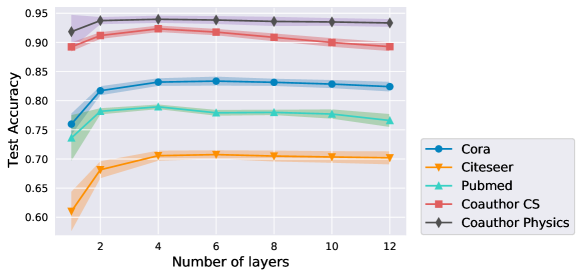
Figure 1: Classification performance of UGDGNN with different propagation depth.

6 Related Works

With the development of various GNN models [29, 21, 54, 60, 56, 5, 9], understanding their working mechanisms has become an important research filed. The graph signal processing tools [14], which have played important roles in some early designs of GNN architectures [2, 12], have been recently used to analyze the properties [46] and to explain the mechanisms [17] of GNNs.

There are some existing works intending to connect existing GNN models with GSD optimization problems [42, 74, 38]. However, all of them focus on investigating the relationship among different FA schemes of GNNs and neglect the indispensible FT steps and none of them relates the GNNs to a bilevel optimization problem. Therefore, their analyses can only be used to interpret one-layer models or parameter-free models. By contrast, our work presents a unified algorithm unrolling perspective on understanding the propagation schemes (including both the FA and FT operations) of GNN models, which is beyond the scope of the existing literatures and also brings much more applications.

Due to space limit, more discussions on related works and future works are presented in Appendix.

7 Conclusion

In this paper, we have established the equivalence between a class of GNN models and unrolled networks for solving GSD problems from a unified algorithm unrolling perspective, with which deeper understandings of the GNNs have been provided. We have shown that training these GNNs is essentially to solve a bilevel optimization problem. Moreover, a novel GNN model called UGDGNN has been proposed and is proved to have favorable expressive power in both the vertex and the spectral domain. Empirical results demonstrate that UGDGNN is able to achieve superior or competitive performance over the state-of-the-art GNNs on various benchmark datasets. The results indicate the promising prospects of designing new models from the algorithm unrolling perspective and leave much space for future explorations.

Checklist

1. For all authors…

   1. Do the main claims made in the abstract and introduction accurately reflect the paper’s contributions and scope? [Yes]

   2. Did you describe the limitations of your work? [Yes]

   3. Did you discuss any potential negative societal impacts of your work? [Yes]

   4. Have you read the ethics review guidelines and ensured that your paper conforms to them? [Yes]

2. If you are including theoretical results…

   1. Did you state the full set of assumptions of all theoretical results? [Yes]

   2. Did you include complete proofs of all theoretical results? [Yes]

3. If you ran experiments…

   1. Did you include the code, data, and instructions needed to reproduce the main experimental results (either in the supplemental material or as a URL)? [Yes]

   2. Did you specify all the training details (e.g., data splits, hyperparameters, how they were chosen)? [Yes]

   3. Did you report error bars (e.g., with respect to the random seed after running experiments multiple times)? [Yes]

   4. Did you include the total amount of compute and the type of resources used (e.g., type of GPUs, internal cluster, or cloud provider)? [Yes]

4. If you are using existing assets (e.g., code, data, models) or curating/releasing new assets…

   1. If your work uses existing assets, did you cite the creators? [Yes]

   2. Did you mention the license of the assets? [No] The assets are open to academic use.

   3. Did you include any new assets either in the supplemental material or as a URL? [No]

   4. Did you discuss whether and how consent was obtained from people whose data you’re using/curating? [N/A]

   5. Did you discuss whether the data you are using/curating contains personally identifiable information or offensive content? [N/A]

5. If you used crowdsourcing or conducted research with human subjects…

   1. Did you include the full text of instructions given to participants and screenshots, if applicable? [N/A]

   2. Did you describe any potential participant risks, with links to Institutional Review Board (IRB) approvals, if applicable? [N/A]

   3. Did you include the estimated hourly wage paid to participants and the total amount spent on participant compensation? [N/A]

Appendix

Appendix A Additional Related Works and Future Directions

Several earlier papers found that the FA step in GCN Kipf and Welling [2017] and SGC Wu et al. [2019] can be seen as the outcome of a special signal smoothing technique called Laplacian smoothing Li et al. [2018], Hoang et al. [2021], Yang et al. [2021a]. Inspired by this observation, there is a line of research focusing on designing novel GNN models based on a “graph regularized optimization problem,” which actually is the vanilla form of the GSD problem given in (1). If a iterative numerical algorithm (e.g., the gradient descent algorithm, matrix inversion algorithm, etc.) is applied to solve this problem, stacking all the iterative steps will naturally lead to a computational model. Since computation over graphs with consecutive propagation layers are involved, such models are all named GNN models. This idea of GNN design (i.e., designing GNNs from iterative algorithms) looks similar to the one proposed in this paper in that both of them originate from GSD optimization problems. Actually they are different in that the GNN models designed from the vanilla GSD problem will finally lead to GNN models without any parameters (except possible parameters included in $p_{\mathsf{pre}}$ and $p_{\mathsf{pos}}$). In other words, no parameters need to be trained in the feature propagation layers in these models. In this paper, we considered a class of popular GNN models which are not originally motivated from the vanilla GSD problem and have learnable parameters in the feature propagation layers. While empirical results have propelled GNN to new heights in recent years, the philosophy behind them is elusive. We firmly believe that practice grounded in theory could help accelerate the GNN research and possibly lead to the discovery of new fields we cannot even conceive of yet. The original intention of this paper is actually to launch an attempt in this direction. We first realized the GSD problem in the area of signal processing over graph shares the same spirit as the GNN model in the area of machine learning over graph. Then, such a connection can actually be made clear through the algorithm unrolling perspective. To the best of our knowledge, this paper is the first attempt of the kind in the literature towards obtaining a holistic understanding of the working mechanisms of existing GNN models.

Among the literature on GNN models designed from the “graph regularized optimization problem,” there are research studies targeting at modifying the signal smoothing term in the optimization problem to strengthen the capability of GNNs. For example, inspired by the idea of trend filtering Wang et al. [2015], authors in Liu et al. [2021b] and Fan et al. [2021] proposed to replace the Laplacian smoothing term (in the form of $\ell_{2}$ norm) with an $\ell_{2,1}$ norm to promote robustness against abnormal edges. Also for robustness pursuit, authors in Yang et al. [2021b] replaced the Laplacian smoothing term with some robustness promoting nonlinear functions over pairwise node distances. Besides promoting smoothness over connected nodes, Zhang et al. [2020a], Zhao and Akoglu [2020] suggested to further promoting the non-smoothness over the disconnected nodes, which is achieved by deducting the sum of distances between disconnected pairs of nodes from the GSD objective. Moreover, Jiang et al. [2022] augments the GSD objective with a fairness term to fight against large topology bias. Most recently, Fu et al. [2021] proposed $p$-Laplacian message passing and ^pGNN, which is capable of dealing with heterophilic graphs and is robust to noisy edges. However, all these techniques amount to designing the FA steps for GNNs, neglecting the power of FT steps, which limits the representation ability of GNNs.

With the proposed algorithm unrolling perspective for understanding GNNs, a wider range of GNNs can be interpreted as solving properly specified GSD problems via unrolled networks. Such an interpretation can inspire more powerful GNN designs that may contain FT steps. Specially, new GNN models can be derived based on other variants of GSD objectives (possibly non-convex or with non-Euclidean structure), other iterative algorithms for problem resolution (e.g., numerical optimization algorithms, numerical linear algebra algorithms, etc.), other unrolling schemes, and so on. Besides, more characteristics of the GNNs can be revealed by further investigating the properties of the underlying GSDs, the iterative algorithms, and/or the unrolling schemes.

Appendix B Societal Impact

The GNN model, a graph-based machine learning method, has achieved great success in many application fields. The unified algorithm unrolling perspective proposed in this paper will benefit the society as it provides a fresh view for understanding these models and can motivate new model designs. For example, one can choose to design a more robust GNN model via designing the unrolled network for a robust GSD problem, which will have significant positive societal impact. There are no evidently negative societal impact as far as we know.

Appendix C Proofs and More Discussions

C.1 Proof of Proposition 3

Proof.

With $\alpha=0$ and $r(\mathbf{H})=\beta\bigl{\|}\mathbf{H}\bigr{\|}_{\mathbf{I}-\mathbf{T}_{\beta}}^{2}$, the GSD problem (2) becomes

$$\underset{\mathbf{H}}{\mathrm{min}} \beta\bigl{\|}\mathbf{B}\mathbf{H}\bigr{\|}_{\mathbf{T}_{\beta}}^{2}+\beta\bigl{\|}\mathbf{H}\bigr{\|}_{\mathbf{I}-\mathbf{T}_{\beta}}^{2}.$$

For the above problem, the $k$-th ($k=1,\ldots,K$) unrolled GD step in (5) accordingly turns to be

$$\mathbf{H}^{(k)} =\mathbf{H}^{(k-1)}-\eta^{(k)}\left(2\beta^{(k)}\mathbf{B}^{T}\mathbf{B}\mathbf{H}^{(k-1)}\mathbf{T}_{\beta}^{(k)}+2\beta^{(k)}\mathbf{H}^{(k-1)}\bigl{(}\mathbf{I}-\mathbf{T}_{\beta}^{(k)}\bigr{)}\right)$$

$$=\mathbf{H}^{(k-1)}-\eta^{(k)}\left(2\beta^{(k)}(\mathbf{I}-\mathbf{A})\mathbf{H}^{(k-1)}\mathbf{T}_{\beta}^{(k)}+2\beta^{(k)}\mathbf{H}^{(k-1)}\bigl{(}\mathbf{I}-\mathbf{T}_{\beta}^{(k)}\bigr{)}\right)$$

$$=\mathbf{H}^{(k-1)}\left(\mathbf{I}-2\eta^{(k)}\beta^{(k)}\mathbf{T}_{\beta}^{(k)}-2\eta^{(k)}\beta^{(k)}\bigl{(}\mathbf{I}-\mathbf{T}_{\beta}^{(k)}\bigr{)}\right)+2\eta^{(k)}\beta^{(k)}\mathbf{A}\mathbf{H}^{(k-1)}\mathbf{T}_{\beta}^{(k)},$$

where in the second line we have used the relation $\mathbf{I}-\mathbf{A}=\mathbf{B}^{T}\mathbf{B}$. By choosing $\eta^{(k)}=\frac{1}{2\beta^{(k)}}$, the unrolled GD step becomes

$$\mathbf{H}^{(k)}=\mathbf{A}\mathbf{H}^{(k-1)}\mathbf{T}_{\beta}^{(k)}.$$

Then, after stacking $K$ unrolled GD steps, we have

$$\bar{\mathbf{X}}=\mathbf{H}^{(K)}=\mathbf{A}^{K}\mathbf{H}^{(0)}\prod_{i=1}^{L}\mathbf{T}_{\beta}^{(k)}.$$

By setting the initial point $\mathbf{H}^{(0)}=\mathbf{X}$ and reparameterizing the weight $\prod_{i=1}^{L}\mathbf{T}_{\beta}^{(k)}=\mathbf{W}$, we obtain the propagation mechanism in SGC, which completes the proof. ∎

In the above proof, we have assumed that the learnable weight matrix $\mathbf{W}$ is induced from the model parameter $\boldsymbol{\Theta}$ in the GSD problem. However, another interesting observation is that it can also be explained into $p_{\mathsf{pre}}$ or $p_{\mathsf{pos}}$. Consider the GSD problem (2) with $\alpha=0$, $\mathbf{T}_{\alpha}=\mathbf{T}_{\beta}=\mathbf{I}$, and $r(\mathbf{H})=0$. By choosing $\eta^{(k)}=\frac{1}{2\beta^{(k)}}$, the $k$-th ($k=1,\ldots,K$) unrolled GD step is correspondingly given by

$$\mathbf{H}^{(k)}=\mathbf{H}^{(k-1)}-2\eta^{(k)}\beta^{(k)}\mathbf{B}^{T}\mathbf{B}\mathbf{H}^{(k-1)}=\mathbf{A}\mathbf{H}^{(k-1)}.$$

Stacking $K$ unrolled GD steps, we get the aggregation mechanism as

$$\mathbf{H}^{(K)}=\mathbf{A}^{K}\mathbf{H}^{(0)}.$$

Setting $\mathbf{H}^{(0)}=\mathbf{X}$ and introducing the transformation matrix $\mathbf{W}$ as a part of $P_{\mathsf{pre}}$ or $P_{\mathsf{pos}}$ lead to the SGC model.

C.2 More Discussions on SGC

Global smoothing properties of the SGC model. From our analysis, since SGC corresponds to a GSD problem with $\alpha=0$ (i.e., no signal fidelity term), it is easy to conclude that the model only performs global smoothing based on the graph topology. Coincidentally, this property has been reported both numerically and theoretically in some existing works Li et al. [2018], Hoang et al. [2021].

Unique limit distributions of the SGC model. It has been discussed in Xu et al. [2018], Klicpera et al. [2019] that under the assumption that the graph is irreducible and aperiodic, the node representations of an infinite layer SGC model will converge to a limit distribution corresponds to the random walk, which only depends on the graph. While based on the GSD problem with the algorithm unrolling perspective, different initial point $\mathbf{H}^{(0)}$ will lead to the same limit result as the GSD problem corresponding to SGC is convex, which exactly coincides with and further corroborates the analyses in Xu et al. [2018], Klicpera et al. [2019].

C.3 Proof of Proposition 4

Proof.

With $\mathbf{T}_{\alpha}=\mathbf{T}_{\beta}=\mathbf{I}$ and $r(\mathbf{H})=0$, the GSD problem becomes the vanilla GSD problem, which has an analytical solution Stanković et al. [2019]. Since $\beta=1-\alpha$, the analytical solution can be obtained by setting the gradient to be zero, i.e.,

$$2\alpha\left(\bar{\mathbf{X}}-\mathbf{X}\right)+2\left(1-\alpha\right)\mathbf{B}^{T}\mathbf{B}\bar{\mathbf{X}}=\mathbf{0},$$

which gives

$$\bar{\mathbf{X}}-\left(1-\alpha\right)\mathbf{A}\bar{\mathbf{X}}=\alpha\mathbf{X},$$

or, equivalently,

$$\bar{\mathbf{X}}=\alpha\left(\mathbf{I}-\left(1-\alpha\right)\mathbf{A}\right)^{-1}\mathbf{X},$$

leading to the exact propagation scheme in PPNP model. Note that PPNP was originally proposed based on the idea of personalized PageRank. Here, we gave another equivalent interpretation based on GSD.

With $\beta=1-\alpha$, $\mathbf{T}_{\alpha}=\mathbf{T}_{\beta}=\mathbf{I}$, and $r(\mathbf{H})=0$, the unrolled GD layer (5) for GSD is

$$\mathbf{H}^{(k)} =\mathbf{H}^{(k-1)}-\eta^{(k)}\left(2\alpha^{(k)}\bigl{(}\mathbf{H}-\mathbf{X}\bigr{)}+2\bigl{(}1-\alpha^{(k)}\bigr{)}\mathbf{B}^{T}\mathbf{B}\mathbf{H}^{(k-1)}\right)$$ (11)

$$=\mathbf{H}^{(k-1)}-\eta^{(k)}\left(2\alpha^{(k)}\bigl{(}\mathbf{H}-\mathbf{X}\bigr{)}+2\bigl{(}1-\alpha^{(k)}\bigr{)}\bigl{(}\mathbf{I}-\mathbf{A}\bigr{)}\mathbf{H}^{(k-1)}\right)$$

$$=\mathbf{H}^{(k-1)}\left(1-2\eta^{(k)}\alpha^{(k)}-2\eta^{(k)}\bigl{(}1-\alpha^{(k)}\bigr{)}\right)+2\eta^{(k)}\bigl{(}1-\alpha^{(k)}\bigr{)}\mathbf{A}\mathbf{H}^{(k-1)}+2\eta^{(k)}\alpha^{(k)}\mathbf{X}.$$

With $\eta^{(k)}=\frac{1}{2}$ and $\alpha^{(k)}=\gamma$, $k=1,\ldots,K$, the $k$-th unrolled GD layer becomes

$$\mathbf{H}^{(k)}=\bigl{(}1-\gamma\bigr{)}\mathbf{A}\mathbf{H}^{(k-1)}+\gamma\mathbf{X},$$

which is exactly the same with the $k$-th propagation layer in APPNP. Note that the PPNP model can be naturally seen as applying infinitely many unrolled GD layers. ∎

C.4 Proof of Proposition 5

Proof.

With $\alpha=\beta$ and $\mathbf{T}_{\alpha}=\mathbf{I}-\mathbf{T}_{\beta}$, the $k$-th ($k=1,\ldots,K$) unrolled GD layer (5) becomes

$$\mathbf{H}^{(k)} =\mathbf{H}^{(k-1)}\left(\mathbf{I}-2\eta^{(k)}\alpha^{(k)}\mathbf{T}_{\alpha}^{(k)}-2\eta^{(k)}\alpha^{(k)}\bigl{(}\mathbf{I}-\mathbf{T}_{\alpha}^{(k)}\bigr{)}\right)$$

$$\hskip 51.21504pt+2\eta^{(k)}\alpha^{(k)}\mathbf{A}\mathbf{H}^{(k-1)}\bigl{(}\mathbf{I}-\mathbf{T}_{\alpha}^{(k)}\bigr{)}+2\eta^{(k)}\alpha^{(k)}\mathbf{X}\mathbf{T}_{\alpha}^{(k)}.$$

By choosing $\eta^{(k)}=\frac{1}{2\alpha^{(k)}}$, we have

$$\mathbf{H}^{(k)}=\mathbf{A}\mathbf{H}^{(k-1)}\bigl{(}\mathbf{I}-\mathbf{T}_{\alpha}^{(k)}\bigr{)}+\mathbf{X}\mathbf{T}_{\alpha}^{(k)}.$$

Stacking $K$ unrolling GD layers, we have

$$\mathbf{H}^{(K)}= \mathbf{A}\mathbf{H}^{(K-1)}\bigl{(}\mathbf{I}-\mathbf{T}_{\alpha}^{(K)}\bigr{)}+\mathbf{X}\mathbf{T}_{\alpha}^{(K)}$$

$$= \mathbf{A}\left(\mathbf{A}\mathbf{H}^{(K-2)}\bigl{(}\mathbf{I}-\mathbf{T}_{\alpha}^{(K-1)}\bigr{)}+\mathbf{X}\mathbf{T}_{\alpha}^{(K-1)}\right)\bigl{(}\mathbf{I}-\mathbf{T}_{\alpha}^{(K)}\bigr{)}+\mathbf{X}\mathbf{T}_{\alpha}^{(K)}$$

$$= \mathbf{A}^{2}\mathbf{H}^{(K-2)}\bigl{(}\mathbf{I}-\mathbf{T}_{\alpha}^{(K-1)}\bigr{)}\bigl{(}\mathbf{I}-\mathbf{T}_{\alpha}^{(K)}\bigr{)}+\mathbf{A}\mathbf{X}\mathbf{T}_{\alpha}^{(K-1)}\bigl{(}\mathbf{I}-\mathbf{T}_{\alpha}^{(K)}\bigr{)}+\mathbf{X}\mathbf{T}_{\alpha}^{(K)}$$

$$= \ldots$$

$$= \mathbf{A}^{K}\mathbf{H}^{(0)}\prod_{k=1}^{K}\bigl{(}\mathbf{I}-\mathbf{T}_{\alpha}^{(k)}\bigr{)}+\sum_{i=1}^{K}\mathbf{A}^{K-i}\mathbf{X}\mathbf{T}_{\alpha}^{(K-i)}\prod_{j=K-i+1}^{K}\bigl{(}\mathbf{I}-\mathbf{T}_{\alpha}^{(j)}\bigr{)}.$$

By reparameterizing $\prod_{k=1}^{K}\bigl{(}\mathbf{I}-\mathbf{T}_{\alpha}^{(k)}\bigr{)}=\mathbf{W}^{(K)}$ and $\mathbf{T}_{\alpha}^{(K-i)}\prod_{j=K-i+1}^{K}\bigl{(}\mathbf{I}-\mathbf{T}_{\alpha}^{(j)}\bigr{)}=\mathbf{W}^{(K-i)}$ for $i=1,\ldots,K$, and setting the initial point $\mathbf{H}^{(0)}=\mathbf{X}$, we obtain the propagation mechanism in the JKNet model. ∎

C.5 Proof of Proposition 6

Proof.

With $\beta=1-\alpha$, $\mathbf{T}_{\alpha}=\mathbf{T}_{\beta}=\mathbf{I}$, and $r(\mathbf{H})=0$, the GPRGNN corresponds to the same GSD problem as APPNP and hence the $k$-th ($k=1,\ldots,K$) unrolled GD layer is the same as (11). By setting $\eta^{(k)}=\frac{1}{2}$, we have

$$\mathbf{H}^{(k)}=\bigl{(}1-\alpha^{(k)}\bigr{)}\mathbf{A}\mathbf{H}^{(k-1)}+\alpha^{(k)}\mathbf{X}.$$

Concatenating $K$ unrolled GD layers, we obtain

$$\mathbf{H}^{(K)} =\bigl{(}1-\alpha^{(K)}\bigr{)}\mathbf{A}\mathbf{H}^{(K-1)}+\alpha^{(K)}\mathbf{X}$$

$$=\bigl{(}1-\alpha^{(K)}\bigr{)}\mathbf{A}\left(\bigl{(}1-\alpha^{(K-1)}\bigr{)}\mathbf{A}\mathbf{H}^{(K-2)}+\alpha^{(K-1)}\mathbf{X}\right)+\alpha^{(K)}\mathbf{X}$$

$$=\bigl{(}1-\alpha^{(K)}\bigr{)}\bigl{(}1-\alpha^{(K-1)}\bigr{)}\mathbf{A}^{2}\mathbf{H}^{(K-2)}+\bigl{(}1-\alpha^{(K)}\bigr{)}\alpha^{(K-1)}\mathbf{A}\mathbf{X}+\alpha^{(K)}\mathbf{X}$$

$$=\cdots$$

$$=\prod_{k=1}^{K}\bigl{(}1-\alpha^{(k)}\bigr{)}\mathbf{A}^{K}\mathbf{H}^{(0)}+\sum_{i=1}^{K}\alpha^{(K-i)}\Biggl{(}\prod_{j=K-i+1}^{K}\bigl{(}1-\alpha^{(j)}\bigr{)}\Biggr{)}\mathbf{A}^{K-i}\mathbf{X}.$$

By reparameterizing $\prod_{k=1}^{K}\bigl{(}1-\alpha^{(k)}\bigr{)}=\gamma^{(K)}$ and $\alpha^{(K-i)}\prod_{j=K-i+1}^{K}\bigl{(}1-\alpha^{(j)}\bigr{)}=\gamma^{(K-i)}$ for $i=1,\ldots,K$, and setting the initial point $\mathbf{H}^{(0)}=\mathbf{X}$, we get the propagation scheme in the GPRGNN model. ∎

C.6 Proof of Proposition 8

Proof.

With $\alpha=0$ and $r(\mathbf{H})=\beta\bigl{\|}\mathbf{H}\bigr{\|}_{\mathbf{I}-\mathbf{T}_{\beta}}^{2}+I_{\{h_{ij}\geq 0,\ \forall i,j\}}(\mathbf{H})$, the $k$-th ($k=1,\ldots,L$) unrolled ProxGD layer (9) becomes

$$\mathbf{H}^{(k)} =\mathrm{ReLU}\biggl{(}\mathbf{H}^{(k-1)}-\eta^{(k)}\Bigl{(}2\beta^{(k)}\mathbf{B}^{T}\mathbf{B}\mathbf{H}^{(k-1)}\mathbf{T}_{\beta}^{(k)}+2\beta^{(k)}\mathbf{H}^{(k-1)}\bigl{(}\mathbf{I}-\mathbf{T}_{\beta}^{(k)}\bigr{)}\Bigr{)}\biggr{)}$$

$$=\mathrm{ReLU}\biggl{(}\mathbf{H}^{(k-1)}\Bigl{(}\mathbf{I}-2\eta^{(k)}\beta^{(k)}\mathbf{T}_{\beta}^{(k)}-2\eta^{(k)}\beta^{(k)}\bigl{(}\mathbf{I}-\mathbf{T}_{\beta}^{(k)}\bigr{)}\Bigr{)}+2\eta^{(k)}\beta^{(k)}\mathbf{A}\mathbf{H}^{(k-1)}\mathbf{T}_{\beta}^{(k)}\biggr{)}.$$

Choosing $\eta^{(k)}=\frac{1}{2\beta^{(k)}}$, we obtain the following feature propagation process

$$\mathbf{H}^{(k)}=\mathrm{ReLU}\bigl{(}\mathbf{A}\mathbf{H}^{(k-1)}\mathbf{T}_{\beta}^{(k)}\bigr{)}.$$

Setting $\mathbf{T}_{\beta}^{(k)}=\mathbf{W}^{(k)}$ recovers a $K$-layer GCN model. ∎

C.7 More Discussions on GCN

Over-smoothing issues of the GCN model. In the literature, it was pointed out that the FA step in GCN, i.e., $\mathbf{A}\mathbf{H}^{(k-1)}$, can be seen as a special form of Laplacian smoothing Li et al. [2018], Yang et al. [2021a]. There were empirical evidence showing that the performance of GCNs can severely degrade as the layer increases. With the above observations, some papers suggested that the performance degradation in deep GCNs is the consequence of the over-smoothing issue Zhao and Akoglu [2020], Cai and Wang [2020], Hoang et al. [2021]. Recently, contrary to the above argument some works argued that the over-smoothing is just an artifact of theoretical analysis and is not the main reason for performance degradation in deep GCNs Yang et al. [2020], Zhou et al. [2021], Cong et al. [2021]. They pointed out that such discrepancy is because the previous over-simplified analyses neglected the FT steps including the multiplication from $\mathbf{W}^{(k)}$ and the nonlinear transformation $\mathrm{ReLU}$. In this paper, based on the algorithm unrolling perspective, in which we treat the consecutive propagation layers in GCN as a whole, we can conclude that GCN cannot be seen as solely performing the goal of signal smoothing due to the regularization term $r(\mathbf{H})$, which supports the above claim that over-smoothing is not the main reason for performance degradation in deep GCNs Yang et al. [2020], Zhou et al. [2021], Cong et al. [2021].

C.8 Proof of Proposition 9

Proof.

With $\beta=1-\alpha$, $\mathbf{T}_{\alpha}=\mathbf{T}_{\beta}$, and $r(\mathbf{H})=\left\|\mathbf{H}\right\|_{\mathbf{I}-\mathbf{T}_{\beta}}^{2}+I_{\{h_{ij}\geq 0,\ \forall i,j\}}(\mathbf{H})$, the $k$-th ($k=1,\ldots,L$) unrolled ProxGD layer (9) becomes

$$\mathbf{H}^{(k)} =\mathrm{ReLU}\biggl{(}\mathbf{H}^{(k-1)}-\eta^{(k)}\Bigl{(}2\bigl{(}1-\beta^{(k)}\bigr{)}\bigl{(}\mathbf{H}-\mathbf{X}\bigr{)}\mathbf{T}_{\beta}^{(k)}+2\beta^{(k)}\mathbf{B}^{T}\mathbf{B}\mathbf{H}^{(k-1)}\mathbf{T}_{\beta}^{(k)}$$

$$\hskip 142.26378pt+2\mathbf{H}^{(k-1)}\bigl{(}\mathbf{I}-\mathbf{T}_{\beta}^{(k)}\bigr{)}\Bigr{)}\biggr{)}$$

$$=\mathrm{ReLU}\biggl{(}\mathbf{H}^{(k-1)}-\eta^{(k)}\Bigl{(}2\bigl{(}1-\beta^{(k)}\bigr{)}\bigl{(}\mathbf{H}-\mathbf{X}\bigr{)}\mathbf{T}_{\beta}^{(k)}+2\beta^{(k)}\bigl{(}\mathbf{I}-\mathbf{A}\bigr{)}\mathbf{H}^{(k-1)}\mathbf{T}_{\beta}^{(k)}$$

$$\hskip 142.26378pt+2\mathbf{H}^{(k-1)}\bigl{(}\mathbf{I}-\mathbf{T}_{\beta}^{(k)}\bigr{)}\Bigr{)}\biggr{)}$$

$$=\mathrm{ReLU}\biggl{(}\mathbf{H}^{(k-1)}\Bigl{(}\mathbf{I}-2\eta^{(k)}\bigl{(}1-\beta^{(k)}\bigr{)}\mathbf{T}_{\beta}^{(k)}-2\eta^{(k)}\beta^{(k)}\mathbf{T}_{\beta}^{(k)}-2\eta^{(k)}\bigl{(}\mathbf{I}-\mathbf{T}_{\beta}^{(k)}\bigr{)}\Bigr{)}$$

$$\hskip 142.26378pt+2\eta^{(k)}\beta^{(k)}\mathbf{A}\mathbf{H}^{(k-1)}\mathbf{T}_{\beta}^{(k)}+2\eta^{(k)}\bigl{(}1-\beta^{(k)}\bigr{)}\mathbf{X}\mathbf{T}_{\beta}^{(k)}\biggr{)}.$$

By choosing $\eta^{(k)}=\frac{1}{2}$, we have

$$\mathbf{H}^{(k)}=\mathrm{ReLU}\Bigl{(}\beta^{(k)}\mathbf{A}\mathbf{H}^{(k-1)}\mathbf{T}_{\beta}^{(k)}+\bigl{(}1-\beta^{(k)}\bigr{)}\mathbf{X}\mathbf{T}_{\beta}^{(k)}\Bigr{)}.$$

Further setting $\beta^{(k)}=\zeta$, $k=1,\ldots,K$ and reparameterizing $\mathbf{T}_{\beta}^{(k)}=\xi\mathbf{W}^{(k)}+\left(1-\xi\right)\mathbf{I}$, we get the GCNII model. ∎

C.9 Proof of Proposition 10

Proof.

Using the ProxGD algorithm with $\alpha^{(k)}=\frac{\gamma}{1-\gamma}\beta^{(k)}$ and stepsize $\eta^{(k)}=\frac{1}{2(1-\alpha^{(k)})}$, we obtain the following iteration:

$$\mathbf{H}^{(k)} =\text{arg}\min_{\mathbf{Y}}\ \bigl{(}1-\beta^{(k)}\bigr{)}\bigl{\|}\mathbf{Y}-\mathbf{X}\bigr{\|}_{2,1}+\frac{1}{2\eta^{(k)}}\bigl{\|}\mathbf{Y}-\bigl{(}\mathbf{H}^{(k-1)}-2\eta^{(k)}\beta^{(k)}(\mathbf{I}-\mathbf{A})\mathbf{H}^{(k-1)}\bigr{)}\bigr{\|}_{F}^{2}$$

$$=\text{arg}\min_{\mathbf{Y}}\ \bigl{(}1-\beta^{(k)}\bigr{)}\bigl{\|}\mathbf{Y}-\mathbf{X}\bigr{\|}_{2,1}$$

$$\hskip 113.81102pt+\frac{1}{2\eta^{(k)}}\bigl{\|}\mathbf{Y}-(1-2\eta^{(k)}\beta^{(k)})\mathbf{H}^{(k-1)}-2\eta^{(k)}\beta^{(k)}\mathbf{A}\mathbf{H}^{(k-1)}\bigr{\|}_{F}^{2}.$$

By choosing $\eta^{(k)}=\frac{1}{2\beta^{(k)}}$, we have

$$\mathbf{H}^{(k)} =\text{arg}\min_{\mathbf{Y}}\ \bigl{(}1-\beta^{(k)}\bigr{)}\bigl{\|}\mathbf{Y}-\mathbf{X}\bigr{\|}_{2,1}+\beta^{(k)}\bigl{\|}\mathbf{Y}-\mathbf{A}\mathbf{H}^{(k-1)}\bigr{\|}_{F}^{2}.$$

The above proximal minimization problem can be computed analytically where the $i$-th row of $\mathbf{H}^{(k)}$, i.e. $\mathbf{h}_{i}^{(k)}$, is given as follows Liu et al. [2021a]:

$$\mathbf{h}_{i}^{(k)}=\mathrm{ReLU}\left(1-\frac{1-\beta^{(k)}}{2\beta^{(k)}||[\mathbf{A}\mathbf{H}^{(k-1)}]_{i}-\mathbf{x}_{i}||_{2}}\right)\bigl{(}[\mathbf{A}\mathbf{H}^{(k-1)}]_{i}-\mathbf{x}_{i}\bigr{)}+\mathbf{x}_{i}.$$

By reparameterizing $\beta^{(k)}=\gamma$ for $k=1,\ldots,K$, we arrive at the AirGNN model. ∎

C.10 Proof of Proposition 11

Proof.

By stacking $K$ unrolled GD layers (5) with initialization $\mathbf{H}^{(0)}=\mathbf{X}$, we have

$$\mathbf{H}^{(K)}= \mathbf{H}^{(K-1)}\bigl{(}\mathbf{I}-2\eta^{(K)}\alpha^{(K)}\mathbf{T}_{\alpha}^{(K)}-2\eta^{(K)}\beta^{(K)}\mathbf{T}_{\beta}^{(K)}\bigr{)}$$

$$\hskip 156.49014pt+2\eta^{(K)}\beta^{(K)}\mathbf{A}\mathbf{H}^{(K-1)}\mathbf{T}_{\beta}^{(K)}+2\eta^{(K)}\alpha^{(K)}\mathbf{X}\mathbf{T}_{\alpha}^{(K)}$$

$$= \Bigl{(}\mathbf{H}^{(K-2)}\bigl{(}\mathbf{I}-2\eta^{(K-1)}\alpha^{(K-1)}\mathbf{T}_{\alpha}^{(K-1)}-2\eta^{(K-1)}\beta^{(K-1)}\mathbf{T}_{\beta}^{(K-1)}\bigr{)}$$

$$\hskip 25.6073pt+2\eta^{(K-1)}\beta^{(K-1)}\mathbf{A}\mathbf{H}^{(K-2)}\mathbf{T}_{\beta}^{(K-1)}+2\eta^{(K-1)}\alpha^{(K-1)}\mathbf{X}\mathbf{T}_{\alpha}^{(K-1)}\Bigr{)}$$

$$\hskip 25.6073pt\times\bigl{(}\mathbf{I}-2\eta^{(K)}\alpha^{(K)}\mathbf{T}_{\alpha}^{(K)}-2\eta^{(K)}\beta^{(K)}\mathbf{T}_{\beta}^{(K)}\bigr{)}+2\eta^{(K)}\alpha^{(K)}\mathbf{X}\mathbf{T}_{\alpha}^{(K)}$$

$$\hskip 25.6073pt+2\eta^{(K)}\beta^{(K)}\mathbf{A}\Bigl{(}\mathbf{H}^{(K-2)}\bigl{(}\mathbf{I}-2\eta^{(K-1)}\alpha^{(K-1)}\mathbf{T}_{\alpha}^{(K-1)}-2\eta^{(K-1)}\beta^{(K-1)}\mathbf{T}_{\beta}^{(K-1)}\bigr{)}$$

$$\hskip 25.6073pt+2\eta^{(K-1)}\beta^{(K-1)}\mathbf{A}\mathbf{H}^{(K-2)}\mathbf{T}_{\beta}^{(K-1)}+2\eta^{(K-1)}\alpha^{(K-1)}\mathbf{X}\mathbf{T}_{\alpha}^{(K-1)}\Bigr{)}\mathbf{T}_{\beta}^{(K)}$$

$$= 2\eta^{(K)}\beta^{(K)}2\eta^{(K-1)}\beta^{(K-1)}\mathbf{A}^{2}\mathbf{H}^{(K-2)}\mathbf{T}_{\beta}^{(K-1)}\mathbf{T}_{\beta}^{(K)}$$

$$\hskip 25.6073pt+\mathbf{A}\mathbf{H}^{(K-2)}\Bigl{(}2\eta^{(K-1)}\beta^{(K-1)}\mathbf{T}_{\beta}^{(K-1)}\bigl{(}\mathbf{I}-2\eta^{(K)}\alpha^{(K)}\mathbf{T}_{\alpha}^{(K)}-2\eta^{(K)}\beta^{(K)}\mathbf{T}_{\beta}^{(K)}\bigr{)}$$

$$\hskip 25.6073pt+2\eta^{(K)}\beta^{(K)}\bigl{(}\mathbf{I}-2\eta^{(K-1)}\alpha^{(K-1)}\mathbf{T}_{\alpha}^{(K-1)}-2\eta^{(K-1)}\beta^{(K-1)}\mathbf{T}_{\beta}^{(K-1)}\bigr{)}\mathbf{T}_{\beta}^{(K)}\Bigr{)}$$

$$\hskip 25.6073pt+\mathbf{H}^{(K-2)}\bigl{(}\mathbf{I}-2\eta^{(K-1)}\alpha^{(K-1)}\mathbf{T}_{\alpha}^{(K-1)}-2\eta^{(K-1)}\beta^{(K-1)}\mathbf{T}_{\beta}^{(K-1)}\bigr{)}$$

$$\hskip 25.6073pt\times\bigl{(}\mathbf{I}-2\eta^{(K)}\alpha^{(K)}\mathbf{T}_{\alpha}^{(K)}-2\eta^{(K)}\beta^{(K)}\mathbf{T}_{\beta}^{(K)}\bigr{)}$$

$$\hskip 25.6073pt+2\eta^{(K)}\beta^{(K)}2\eta^{(K-1)}\alpha^{(K-1)}\mathbf{A}\mathbf{X}\mathbf{T}_{\alpha}^{(K-1)}\mathbf{T}_{\beta}^{(K)}+\mathbf{X}\Bigl{(}2\eta^{(K)}\alpha^{(K)}\mathbf{T}_{\alpha}^{(K)}$$

$$\hskip 25.6073pt+2\eta^{(K-1)}\alpha^{(K-1)}\mathbf{T}_{\alpha}^{(K-1)}\bigl{(}\mathbf{I}-2\eta^{(K)}\alpha^{(K)}\mathbf{T}_{\alpha}^{(K)}-2\eta^{(K)}\beta^{(K)}\mathbf{T}_{\beta}^{(K)}\bigr{)}\Bigr{)}$$

$$= \mathbf{A}^{K}\mathbf{X}\prod_{k=1}^{K}2\eta^{(k)}\beta^{(k)}\mathbf{T}_{\beta}^{(k)}$$

$$+\cdots$$

$$+\mathbf{A}^{0}\mathbf{X}\biggl{(}2\eta^{(K)}\alpha^{(K)}\mathbf{T}_{\alpha}^{(K)}+\Bigl{(}2\eta^{(K-1)}\alpha^{(K-1)}\mathbf{T}_{\alpha}^{(K-1)}+\bigl{(}2\eta^{(K-2)}\alpha^{(K-2)}\mathbf{T}_{\alpha}^{(K-2)}+\cdots\bigr{)}$$

$$\times\bigl{(}\mathbf{I}-2\eta^{(K-1)}\alpha^{(K-1)}\mathbf{T}_{\alpha}^{(K-1)}-2\eta^{(K-1)}\beta^{(K-1)}\mathbf{T}_{\beta}^{(K-1)}\bigr{)}\Bigr{)}$$

$$\times\bigl{(}\mathbf{I}-2\eta^{(K)}\alpha^{(K)}\mathbf{T}_{\alpha}^{(K)}-2\eta^{(K)}\beta^{(K)}\mathbf{T}_{\beta}^{(K)}\bigr{)}\biggr{)}.$$

To reduce the complexity of the unrolled network, we reparameterize it into the following form

$$\bar{\mathbf{X}}=\sum_{k=0}^{K}\gamma^{(k)}\mathbf{A}^{k}\mathbf{X}\left(\zeta^{(k)}\mathbf{I}+\xi^{(k)}\mathbf{W}^{(k)}\right)$$

with $\gamma^{(k)}$, $\zeta^{(k)}$, $\xi^{(k)}$, and $\mathbf{W}^{(k)}$ being the learnable model parameters. Note that we have left the identity matrix outside of the weight matrix to promote the optimal weight matrices with small norms and reduce the model complexity, which guarantees better generalization ability Cong et al. [2021] and has been shown to be useful particularly in semi-supervised learning tasks Chen et al. [2020]. In the experiments, we further set $\xi^{(k)}=1-\zeta^{(k)}$ to reduce the parameter space. Note that such a further restriction does not change the expressive power of UGDGNN. Similarly, one can also choose to reduce the parameter $\gamma^{(k)}$ by merging it into $\zeta^{(k)}$ and $\xi^{(k)}$. ∎

C.11 Proof of Theorem 12 (Expressive Power Analysis of UGDGNN in the Spectral Domain)

Proof.

The propagation scheme of a $K$ layer UGDGNN is

$$\bar{\mathbf{X}} =\sum_{k=0}^{K}\gamma^{(k)}\mathbf{A}^{k}\mathbf{X}\bigl{(}\zeta^{(k)}\mathbf{I}+\xi^{(k)}\mathbf{W}^{(k)}\bigr{)}$$

$$=\sum_{k=0}^{K}\gamma^{(k)}\bigl{(}\mathbf{I}-\mathbf{L}\bigr{)}^{k}\mathbf{X}\bigl{(}\zeta^{(k)}\mathbf{I}+\xi^{(k)}\mathbf{W}^{(k)}\bigr{)}.$$ (12)

On the other hand, an order $K$ polynomial frequency filter Shuman et al. [2013] can be expressed as

$$\left(\sum_{k=0}^{K}\theta_{k}\mathbf{L}^{k}\right)\mathbf{X} =\left(\sum_{k=0}^{K}\theta_{k}\left(\mathbf{I}-\left(\mathbf{I}-\mathbf{L}\right)\right)^{k}\right)\mathbf{X}$$

$$=\left(\sum_{k=0}^{K}\theta_{k}\left(\sum_{i=0}^{k}\left(-1\right)^{i}\left(\begin{array}[]{c}k\\ i\end{array}\right)\left(\mathbf{I}-\mathbf{L}\right)^{i}\right)\right)\mathbf{X}$$ (15)

$$=\sum_{k=0}^{K}\sum_{i=0}^{k}\theta_{k}\left(-1\right)^{i}\left(\begin{array}[]{c}k\\ i\end{array}\right)\left(\mathbf{I}-\mathbf{L}\right)^{i}\mathbf{X}$$ (18)

$$=\sum_{i=0}^{K}\left(\sum_{k=i}^{K}\theta_{k}\left(-1\right)^{i}\left(\begin{array}[]{c}k\\ i\end{array}\right)\right)\left(\mathbf{I}-\mathbf{L}\right)^{i}\mathbf{X},$$ (21)

where $\left(\begin{array}[]{c}k\\ i\end{array}\right)$ represents the number of combinations for “$k$ choose $i$” and in the last line we have exchanged the order of the double summations.

Comparing (12) and (21), the UGDGNN model with $\gamma^{(i)}=\sum_{k=i}^{K}\theta_{k}\left(-1\right)^{i}\left(\begin{array}[]{c}k\\ i\end{array}\right)$, $\zeta^{(i)}=1$, and $\xi^{(i)}=0$ for $i=1,\ldots,K$ is equivalent to a polynomial frequency filter, which completes the proof. ∎

Appendix D Discussions on the Expressive Power of UGDGNN in the Vertex Domain

Since the UGDGNN model is derived based on concatenating the general unrolled GD layers (5), it is expected to be more expressive than other GNN models explained via unrolled GD layers with specific parameters. In the following, we give the connections between UGDGNN and several existing GNNs that can be seen as unrolled GD networks.

• The SGC model can be seen as a UGDGNN with $\gamma^{(K)}=1$, $\zeta^{(K)}=0$, $\xi^{(K)}=1$, and $\gamma^{(k)}=0$ for $k=1,\ldots,K-1$.

• The APPNP model can be seen as a UGDGNN with $\zeta^{(k)}=1$ and $\xi^{(k)}=0$, $k=1,\ldots,K$, while $\gamma^{(K)}=\left(1-\alpha\right)^{K}$ and $\gamma^{(k)}=\alpha\sum_{k=0}^{K-1}\left(1-\alpha\right)^{k}$ for $k=1,\ldots,K-1$.

• The JKNet model can be seen as a UGDGNN with $\gamma^{(k)}=1$, $\zeta^{(k)}=0$, and $\xi^{(k)}=1$ for $k=1,\ldots,K$.

• The GPRGNN model can be seen as a UGDGNN with $\zeta^{(k)}=1$ and $\xi^{(k)}=0$ for $k=1,\ldots,K$.

Appendix E Expressive Power Analysis of Existing GNNs in the Spectral Domain

E.1 Expressive Power of SGC and GCN

It has been shown that a $K$-layer SGC act as a frequency filter of order $K$ with fixed coefficients Wu et al. [2019], Klicpera et al. [2019], Chen et al. [2020]. Recalling that a $K$-layer SGC is

$$\bar{\mathbf{X}}=\mathbf{A}^{K}\mathbf{X}\mathbf{W}=\left(\mathbf{I}-\mathbf{L}\right)^{K}\mathbf{X}\mathbf{W}=\sum_{k=0}^{K}\left(-1\right)^{k}\left(\begin{array}[]{c}K\\ k\end{array}\right)\mathbf{L}^{k}\mathbf{X}\mathbf{W}.$$

It can be seen as an order-$K$ frequency filter with fixed coefficients $\theta_{k}=\left(-1\right)^{k}\left(\begin{array}[]{c}K\\ k\end{array}\right)$, $k=1,\ldots,K$ and $\mathbf{W}=\mathbf{I}$.

If we neglect the activation functions in GCN or, equivalently, assume all the intermediate node representations are positive and set all the weight matrices to be identity matrices, the GCN model becomes the SGC model, and therefore it also act as an order-$K$ frequency filter with fixed coefficients. Such a frequency filter with fixed coefficients inevitably has limited expressive power.

E.2 Expressive Power of APPNP

The propagation scheme of a $K$-layer APPNP is

$$\bar{\mathbf{X}}=\mathbf{H}^{(K)},\ \ \mathbf{H}^{(k)}=\left(1-\alpha\right)\mathbf{A}\mathbf{H}^{(k-1)}+\alpha\mathbf{X},\ \ k=1,\ldots,K.$$

With $\mathbf{H}^{(0)}=\mathbf{X}$, by stacking the $K$ layers together, we have Klicpera et al. [2019]

$$\bar{\mathbf{X}}=\left(\left(1-\alpha\right)^{K}\mathbf{A}^{K}+\alpha\sum_{k=0}^{K-1}\left(1-\alpha\right)^{k}\mathbf{A}^{k}\right)\mathbf{X}.$$

Suppose $K$ is sufficiently large, we have $\left(1-\alpha\right)^{K}\rightarrow 0$, leading to

$$\bar{\mathbf{X}} =\alpha\sum_{k=0}^{K-1}\left(1-\alpha\right)^{k}\mathbf{A}^{k}\mathbf{X}$$

$$=\alpha\sum_{k=0}^{K-1}\left(1-\alpha\right)^{k}\left(\mathbf{I}-\mathbf{L}\right)^{k}\mathbf{X}$$

$$=\alpha\sum_{k=0}^{K-1}\left(1-\alpha\right)^{k}\sum_{i=0}^{k}\left(\begin{array}[]{c}k\\ i\end{array}\right)\left(-1\right)^{i}\mathbf{L}^{i}\mathbf{X}$$

$$=\sum_{k=0}^{K-1}\sum_{i=0}^{k}\alpha\left(1-\alpha\right)^{k}\left(\begin{array}[]{c}k\\ i\end{array}\right)\left(-1\right)^{i}\mathbf{L}^{i}\mathbf{X}$$

$$=\sum_{i=0}^{K-1}\sum_{k=i}^{K-1}\alpha\left(1-\alpha\right)^{k}\left(\begin{array}[]{c}k\\ i\end{array}\right)\left(-1\right)^{i}\mathbf{L}^{i}\mathbf{X}.$$

Therefore, we can conclude that the APPNP model act as an order-$K$ frequency filter with fixed coefficients $\theta_{k}=\sum_{k=k}^{K-1}\alpha\left(1-\alpha\right)^{k}\left(\begin{array}[]{c}k\\ k\end{array}\right)\left(-1\right)^{k}$, $k=1,\ldots,K$, and $\theta_{K}=0$.

E.3 Expressive Power of GCNII

Recalling that the propagation scheme in GCNII is

$$\bar{\mathbf{X}}=\mathbf{H}^{(K)},\ \ \mathbf{H}^{(k)}=\mathrm{ReLU}\Bigl{(}\bigl{(}\beta\mathbf{A}\mathbf{H}^{(k-1)}+(1-\beta)\mathbf{X}\bigr{)}\bigl{(}\gamma\mathbf{W}^{(k)}+(1-\gamma)\mathbf{I}\bigr{)}\Bigr{)},\ \ k=1,\ldots,K.$$

Similar to the analysis for GCN, we neglect the activation functions. Assuming $\beta=\frac{1}{2}$ and $\gamma\mathbf{W}^{(k)}+(1-\gamma)\mathbf{I}=2w^{(k)}\mathbf{I}$, we have

$$\mathbf{H}^{(k)} =\bigl{(}\mathbf{A}\mathbf{H}^{(k-1)}+\mathbf{X}\bigr{)}w^{(k)}\mathbf{I}$$

$$=w^{(k)}\bigl{(}\mathbf{I}-\mathbf{L}\bigr{)}\mathbf{H}^{(k-1)}+w^{(k)}\mathbf{X}.$$

Stacking $K$ layers and setting $\mathbf{H}^{(0)}=\mathbf{X}$, we obtain

$$\bar{\mathbf{X}}=\sum_{k=0}^{K}\left(\prod_{k=K-k}^{K}w^{(k)}\right)\left(\mathbf{I}-\mathbf{L}\right)^{k}\mathbf{X}.$$

As shown in Appendix E, a frequency filter of order-$K$ can be expressed as

$$\left(\sum_{k=0}^{K}\theta_{k}\mathbf{L}^{k}\right)\mathbf{X}=\sum_{i=0}^{K}\left(\sum_{k=i}^{K}\theta_{k}\left(-1\right)^{i}\left(\begin{array}[]{c}k\\ i\end{array}\right)\right)\left(\mathbf{I}-\mathbf{L}\right)^{i}\mathbf{X}.$$

Comparing the two equations above, we can find a GCNII model can express an arbitrary frequency filter with nonzero coefficients with Chen et al. [2020]

$$w^{(k)}=\frac{\sum_{k=i}^{K}\theta_{k}\left(-1\right)^{i}\left(\begin{array}[]{c}k\\ i\end{array}\right)}{\sum_{k=i-1}^{K}\theta_{k}\left(-1\right)^{i-1}\left(\begin{array}[]{c}k\\ i-1\end{array}\right)}.$$

As for the JKNet model and the GPRGNN model, they have the same spectral expressive power as UGDGNN and can be proved in a fashion similar as in Appendix C.11.

From the above analyses, we can conclude that UGDGNN, JKNet, GPRGNN has better spectral expressive power in comparison with SGC, GCN, APPNP, and GCNII.

Appendix F Experimental Details

F.1 Datasets

To ensure a fair comparison, we choose the same data splits as in Yang et al. [2016] for the Cora, CiteSeer, and PubMed datasets Sen et al. [2008], i.e., we use 20 labeled nodes per class as the training set, 500 nodes as the validation set, and 1000 nodes as the test set. For co-authorship and co-purchase graph datasets Shchur et al. [2018], we use 20 labeled nodes per class as the training set, 30 node per class as the validation set, and the rest as the test set. For OGBN-ArXiv Hu et al. [2020], we use the standard leaderboard splitting, i.e. paper published until 2017 for training, papers published in 2018 for validation, and papers published since 2019 for testing. The statistics for all the benchmark datasets are summarized in Table 3.

Table 3: Statistics of benchmark datasets.

Dataset	Nodes	Edges	Features	Classes	Training Nodes	Validation Nodes	Test Nodes
Cora	2708	5429	1433	7	20 per class	500	1000
Citeseer	3327	4732	3703	6	20 per class	500	1000
Pubmed	19717	44338	500	3	20 per class	500	1000
Coauthor CS	18333	81894	6805	15	20 per class	30 per class	Rest nodes
Coauthor Physics	34493	247962	8415	5	20 per class	30 per class	Rest nodes
Amazon Photo	7487	119043	745	8	20 per class	30 per class	Rest nodes
OGBN-ArXiv	169343	1166243	128	40	Papers until 2017	Papers in 2018	Paper since 2019

F.2 Implementation Details

In this paper, experiments are conducted either on an 11G RTX 2080Ti GPU or on a 48G RTX A6000 GPU. The implementation is based on PyTorch Geometric Fey and Lenssen [2019] and the code is provided in the supplemental materials. We train all the GNN models with a maximum of 1000 training epochs and the Adam optimizer Kingma and Ba [2015] is adopted for model training. The reported results are all averaged values over ten times of independent repetitions.

To ensure fair comparisons, we fix the size of hidden layers uniformly as 64 for all models and on all datasets. Other hyperparameters are tuned with grid search based on the validation results. Actually, we have observed that some models can achieve better results than the original results reported. For all models, the learning rate is chosen from {0.005, 0.01, 0.05} and the dropout rate is chosen from {0.1, 0.5, 0.8}. We also apply the $\ell_{2}$ regularization technique on the weight parameters for all models, where the weight decay parameter is chosen from {0, 5e-5, 5e-4}. The layers for GCN and SGC are set as 2, while the layers for other models are selected from {5, 10, 20}. The teleport probability in APPNP and GPRGNN (note that teleport probability is used just for initialization in GPRGNN) is selected from {0.1, 0.2, 0.5, 0.9}. The best sets of hyperparameters for all models on all datasets are are summarized in Table 4. Note that the hyperparameters used for generating the results in Figure 1 are the same as those in Table 2 (from the main body of the paper). That is, hyperparameters like learning rate, weight decay, and dropout are not specifically tuned for different layers. Therefore, there is a chance that the results reported in Figure 1 can be further improved by carefully tuning the hyperparameters.

Table 4: Hyperparameters (for Table 2 of the main paper) selected based on the validation set.

Dataset	Hyperparameter	GCN	SGC	APPNP	JKNet	GCNII	DAGNN	GPRGNN	UGDGNN
Cora	learning rate	0.01	0.05	0.005	0.05	0.01	0.01	0.01	0.005
	weight decay	5e-4	5e-5	5e-5	5e-4	5e-4	5e-4	5e-4	5e-4
	dropout	0.8	*	0.1	0.5	0.5	0.8	0.5	0.8
	layer	*	*	5	5	20	10	10	5
	alpha	*	*	0.1	*	*	*	0.1	*
CiteSeer	learning rate	0.05	0.05	0.01	0.05	0.05	0.005	0.005	0.01
	weight decay	5e-4	5e-5	5e-4	5e-4	0	5e-4	5e-4	5e-5
	dropout	0.5	*	0.1	0.8	0.5	0.5	0.5	0.8
	layer	*	*	5	5	20	5	10	5
	alpha	*	*	0.2	*	*	*	0.1	*
PubMed	learning rate	0.005	0.05	0.005	0.05	0.05	0.005	0.01	0.005
	weight decay	5e-4	5e-5	5e-4	5e-4	0	5e-4	5e-4	5e-4
	dropout	0.1	*	0.1	0.8	0.5	0.8	0.1	0.1
	layer	*	*	5	5	20	20	20	5
	alpha	*	*	0.2	*	*	*	0.5	*
CS	learning rate	0.005	0.005	0.05	0.05	0.01	0.005	0.01	0.005
	weight decay	5e-5	5e-5	5e-5	5e-5	5e-4	5e-4	0	5e-5
	dropout	0.8	*	0.8	0.8	0.1	0.8	0.5	0.1
	layer	*	*	20	5	20	10	5	5
	alpha	*	*	0.2	*	*	*	0.1	*
Physics	learning rate	0.01	0.005	0.005	0.01	0.05	0.005	0.005	0.005
	weight decay	0	0	5e-4	0	5e-4	0	5e-5	0
	dropout	0.5	*	0.1	0.8	0.5	0.8	0.1	0.8
	layer	*	*	10	5	20	5	20	5
	alpha	*	*	0.1	*	*	*	0.5	*
Photo	learning rate	0.01	0.05	0.05	0.05	0.01	0.05	0.005	0.005
	weight decay	0	0	5e-5	5e-5	5e-5	5e-4	5e-4	0
	dropout	0.8	*	0.1	0.5	0.1	0.5	0.1	0.5
	layer	*	*	10	10	5	5	5	5
	alpha	*	*	0.1	*	*	*	0.1	*
ArXiv	learning rate	0.005	0.05	0.01	0.005	0.005	0.005	0.01	0.005
	weight decay	0	0	0	5e-4	5e-4	0	5e-4	0
	dropout	0.1	*	0.1	0.1	0.1	0.1	0.1	0.1
	layer	*	*	5	10	10	20	5	10
	alpha	*	*	0.1	*	*	*	0.1	*

References

- Borgerding and Schniter [2016] Mark Borgerding and Philip Schniter. Onsager-corrected deep learning for sparse linear inverse problems. In 2016 IEEE Global Conference on Signal and Information Processing (GlobalSIP), pages 227–231. IEEE, 2016.
- Bruna et al. [2014] Joan Bruna, Wojciech Zaremba, Arthur Szlam, and Yann LeCun. Spectral networks and deep locally connected networks on graphs. In International Conference on Learning Representations, 2014.
- Cai and Wang [2020] Chen Cai and Yusu Wang. A note on over-smoothing for graph neural networks. arXiv preprint arXiv:2006.13318, 2020.
- Cappart et al. [2021] Quentin Cappart, Didier Chételat, Elias Khalil, Andrea Lodi, Christopher Morris, and Petar Veličković. Combinatorial optimization and reasoning with graph neural networks. arXiv preprint arXiv:2102.09544, 2021.
- Chen et al. [2020] Ming Chen, Zhewei Wei, Zengfeng Huang, Bolin Ding, and Yaliang Li. Simple and deep graph convolutional networks. In International Conference on Machine Learning, pages 1725–1735. PMLR, 2020.
- Chen et al. [2021a] Tianlong Chen, Xiaohan Chen, Wuyang Chen, Howard Heaton, Jialin Liu, Zhangyang Wang, and Wotao Yin. Learning to optimize: A primer and a benchmark. arXiv preprint arXiv:2103.12828, 2021a.
- Chen et al. [2021b] Tianlong Chen, Kaixiong Zhou, Keyu Duan, Wenqing Zheng, Peihao Wang, Xia Hu, and Zhangyang Wang. Bag of tricks for training deeper graph neural networks: A comprehensive benchmark study. arXiv preprint arXiv:2108.10521, 2021b.
- Chen et al. [2018] Xiaohan Chen, Jialin Liu, Zhangyang Wang, and Wotao Yin. Theoretical linear convergence of unfolded ISTA and its practical weights and thresholds. In Advances in Neural Information Processing Systems, pages 9079–9089, 2018.
- Chien et al. [2021] Eli Chien, Jianhao Peng, Pan Li, and Olgica Milenkovic. Adaptive universal generalized pagerank graph neural network. In International Conference on Learning Representations, 2021.
- Combettes and Pesquet [2020] Patrick L Combettes and Jean-Christophe Pesquet. Deep neural network structures solving variational inequalities. Set-Valued and Variational Analysis, pages 1–28, 2020.
- Cong et al. [2021] Weilin Cong, Morteza Ramezani, and Mehrdad Mahdavi. On provable benefits of depth in training graph convolutional networks. Advances in Neural Information Processing Systems, 34, 2021.
- Defferrard et al. [2016] Michaël Defferrard, Xavier Bresson, and Pierre Vandergheynst. Convolutional neural networks on graphs with fast localized spectral filtering. Advances in Neural Information Processing Systems, 29:3844–3852, 2016.
- Dempe and Zemkoho [2020] Stephan Dempe and Alain Zemkoho. Bilevel optimization. Springer, 2020.
- Dong et al. [2020] Xiaowen Dong, Dorina Thanou, Laura Toni, Michael Bronstein, and Pascal Frossard. Graph signal processing for machine learning: A review and new perspectives. IEEE Signal Processing Magazine, 37(6):117–127, 2020.
- Fan et al. [2021] Wenqi Fan, Xiaorui Liu, Wei Jin, Xiangyu Zhao, Jiliang Tang, and Qing Li. Graph trend networks for recommendations. arXiv preprint arXiv:2108.05552, 2021.
- Fey and Lenssen [2019] Matthias Fey and Jan E. Lenssen. Fast graph representation learning with PyTorch Geometric. In ICLR Workshop on Representation Learning on Graphs and Manifolds, 2019.
- Fu et al. [2020] Guoji Fu, Yifan Hou, Jian Zhang, Kaili Ma, Barakeel Fanseu Kamhoua, and James Cheng. Understanding graph neural networks from graph signal denoising perspectives. arXiv preprint arXiv:2006.04386, 2020.
- Fu et al. [2021] Guoji Fu, Peilin Zhao, and Yatao Bian. -laplacian based graph neural networks. arXiv preprint arXiv:2111.07337, 2021.
- Gilmer et al. [2017] Justin Gilmer, Samuel S Schoenholz, Patrick F Riley, Oriol Vinyals, and George E Dahl. Neural message passing for quantum chemistry. In International Conference on Machine Learning, pages 1263–1272. PMLR, 2017.
- Gregor and LeCun [2010] Karol Gregor and Yann LeCun. Learning fast approximations of sparse coding. In International Conference on Machine Learning, pages 399–406, 2010.
- Hamilton et al. [2017] William L Hamilton, Rex Ying, and Jure Leskovec. Inductive representation learning on large graphs. In Advances in Neural Information Processing Systems, pages 1025–1035, 2017.
- Hershey et al. [2014] John R Hershey, Jonathan Le Roux, and Felix Weninger. Deep unfolding: Model-based inspiration of novel deep architectures. arXiv preprint arXiv:1409.2574, 2014.
- Hoang et al. [2021] NT Hoang, Takanori Maehara, and Tsuyoshi Murata. Revisiting graph neural networks: Graph filtering perspective. In International Conference on Pattern Recognition, pages 8376–8383. IEEE, 2021.
- Hu et al. [2020] Weihua Hu, Matthias Fey, Marinka Zitnik, Yuxiao Dong, Hongyu Ren, Bowen Liu, Michele Catasta, and Jure Leskovec. Open graph benchmark: Datasets for machine learning on graphs. Advances in Neural Information Processing Systems, 2020.
- Huber [2004] Peter J Huber. Robust statistics, volume 523. John Wiley & Sons, 2004.
- Jiang et al. [2022] Zhimeng Jiang, Xiaotian Han, Chao Fan, Zirui Liu, Na Zou, Ali Mostafavi, and Xia Hu. Fmp: Toward fair graph message passing against topology bias. arXiv preprint arXiv:2202.04187, 2022.
- Kalofolias [2016] Vassilis Kalofolias. How to learn a graph from smooth signals. In Artificial Intelligence and Statistics, pages 920–929. PMLR, 2016.
- Kingma and Ba [2015] Diederik P Kingma and Jimmy Ba. Adam: A method for stochastic optimization. In International Conference on Learning Representations (ICLR), 2015.
- Kipf and Welling [2017] Thomas N. Kipf and Max Welling. Semi-supervised classification with graph convolutional networks. In International Conference on Learning Representations, 2017.
- Klicpera et al. [2019] Johannes Klicpera, Aleksandar Bojchevski, and Stephan Günnemann. Predict then propagate: Graph neural networks meet personalized pagerank. In International Conference on Learning Representations, 2019.
- Kloumann et al. [2017] Isabel M Kloumann, Johan Ugander, and Jon Kleinberg. Block models and personalized pagerank. Proceedings of the National Academy of Sciences, 114(1):33–38, 2017.
- Li et al. [2019] Pan Li, I Chien, and Olgica Milenkovic. Optimizing generalized pagerank methods for seed-expansion community detection. Advances in Neural Information Processing Systems, 32:11710–11721, 2019.
- Li et al. [2018] Qimai Li, Zhichao Han, and Xiao-Ming Wu. Deeper insights into graph convolutional networks for semi-supervised learning. In AAAI Conference on Artificial Intelligence, 2018.
- Liu and Chen [2019] Jialin Liu and Xiaohan Chen. Alista: Analytic weights are as good as learned weights in lista. In International Conference on Learning Representations (ICLR), 2019.
- Liu et al. [2020] Meng Liu, Hongyang Gao, and Shuiwang Ji. Towards deeper graph neural networks. In ACM SIGKDD International Conference on Knowledge Discovery & Data Mining, pages 338–348, 2020.
- Liu et al. [2021a] Xiaorui Liu, Jiayuan Ding, Wei Jin, Han Xu, Yao Ma, Zitao Liu, and Jiliang Tang. Graph neural networks with adaptive residual. In Advances in Neural Information Processing Systems, 2021a.
- Liu et al. [2021b] Xiaorui Liu, Wei Jin, Yao Ma, Yaxin Li, Hua Liu, Yiqi Wang, Ming Yan, and Jiliang Tang. Elastic graph neural networks. In International Conference on Machine Learning, pages 6837–6849. PMLR, 2021b.
- Ma et al. [2021] Yao Ma, Xiaorui Liu, Tong Zhao, Yozen Liu, Jiliang Tang, and Neil Shah. A unified view on graph neural networks as graph signal denoising. In ACM International Conference on Information & Knowledge Management, pages 1202–1211, 2021.
- Monga et al. [2021] Vishal Monga, Yuelong Li, and Yonina C Eldar. Algorithm unrolling: Interpretable, efficient deep learning for signal and image processing. IEEE Signal Processing Magazine, 38(2):18–44, 2021.
- Newman [2018] Mark Newman. Networks. Oxford University Press, 2018.
- Page et al. [1998] Lawrence Page, Sergey Brin, Rajeev Motwani, and Terry Winograd. The pagerank citation ranking: Bringing order to the web. Technical report, Stanford InfoLab, 1998.
- Pan et al. [2020] Xuran Pan, Shiji Song, and Gao Huang. A unified framework for convolution-based graph neural networks. https://openreview.net/forum?id=zUMD–Fb9Bt, 2020.
- Papyan et al. [2017] Vardan Papyan, Yaniv Romano, and Michael Elad. Convolutional neural networks analyzed via convolutional sparse coding. The Journal of Machine Learning Research, 18(1):2887–2938, 2017.
- Pei et al. [2020] Hongbin Pei, Bingzhe Wei, Kevin Chen-Chuan Chang, Yu Lei, and Bo Yang. Geom-GCN: Geometric graph convolutional networks. In International Conference on Learning Representations, 2020.
- Rong et al. [2020] Yu Rong, Yatao Bian, Tingyang Xu, Weiyang Xie, Ying Wei, Wenbing Huang, and Junzhou Huang. Self-supervised graph transformer on large-scale molecular data. Advances in Neural Information Processing Systems, 33:12559–12571, 2020.
- Ruiz et al. [2021] Luana Ruiz, Fernando Gama, and Alejandro Ribeiro. Graph neural networks: Architectures, stability, and transferability. Proceedings of the IEEE, 109(5):660–682, 2021.
- Satorras and Estrach [2018] Victor Garcia Satorras and Joan Bruna Estrach. Few-shot learning with graph neural networks. In International Conference on Learning Representations, 2018.
- Sen et al. [2008] Prithviraj Sen, Galileo Namata, Mustafa Bilgic, Lise Getoor, Brian Galligher, and Tina Eliassi-Rad. Collective classification in network data. AI Magazine, 29(3):93–93, 2008.
- Shchur et al. [2018] Oleksandr Shchur, Maximilian Mumme, Aleksandar Bojchevski, and Stephan Günnemann. Pitfalls of graph neural network evaluation. arXiv preprint arXiv:1811.05868, 2018.
- Shuman et al. [2013] David I Shuman, Sunil K Narang, Pascal Frossard, Antonio Ortega, and Pierre Vandergheynst. The emerging field of signal processing on graphs: Extending high-dimensional data analysis to networks and other irregular domains. IEEE Signal Processing Magazine, 30(3):83–98, 2013.
- Srebro and Jaakkola [2003] Nathan Srebro and Tommi Jaakkola. Weighted low-rank approximations. In International Conference on Machine Learning, pages 720–727, 2003.
- Stanković et al. [2019] Ljubiša Stanković, Miloš Daković, and Ervin Sejdić. Introduction to graph signal processing. In Vertex-Frequency Analysis of Graph Signals, pages 3–108. Springer, 2019.
- Tolstaya et al. [2020] Ekaterina Tolstaya, Fernando Gama, James Paulos, George Pappas, Vijay Kumar, and Alejandro Ribeiro. Learning decentralized controllers for robot swarms with graph neural networks. In Conference on Robot Learning, pages 671–682. PMLR, 2020.
- Veličković et al. [2018] Petar Veličković, Guillem Cucurull, Arantxa Casanova, Adriana Romero, Pietro Liò, and Yoshua Bengio. Graph attention networks. In International Conference on Learning Representations, 2018.
- Wang et al. [2015] Yu-Xiang Wang, James Sharpnack, Alex Smola, and Ryan Tibshirani. Trend filtering on graphs. In Artificial Intelligence and Statistics, pages 1042–1050. PMLR, 2015.
- Wu et al. [2019] Felix Wu, Amauri Souza, Tianyi Zhang, Christopher Fifty, Tao Yu, and Kilian Weinberger. Simplifying graph convolutional networks. In International Conference on Machine Learning, pages 6861–6871. PMLR, 2019.
- Wu et al. [2021] Lingfei Wu, Yu Chen, Kai Shen, Xiaojie Guo, Hanning Gao, Shucheng Li, Jian Pei, and Bo Long. Graph neural networks for natural language processing: A survey. arXiv preprint arXiv:2106.06090, 2021.
- Wu et al. [2022] Lingfei Wu, Peng Cui, Jian Pei, and Liang Zhao. Graph Neural Networks: Foundations, Frontiers, and Applications. Springer, Singapore, 2022.
- Wu et al. [2020] Zonghan Wu, Shirui Pan, Fengwen Chen, Guodong Long, Chengqi Zhang, and S Yu Philip. A comprehensive survey on graph neural networks. IEEE Transactions on Neural Networks and Learning Systems, 32(1):4–24, 2020.
- Xu et al. [2018] Keyulu Xu, Chengtao Li, Yonglong Tian, Tomohiro Sonobe, Ken-ichi Kawarabayashi, and Stefanie Jegelka. Representation learning on graphs with jumping knowledge networks. In International Conference on Machine Learning, pages 5453–5462. PMLR, 2018.
- Yang et al. [2020] Chaoqi Yang, Ruijie Wang, Shuochao Yao, Shengzhong Liu, and Tarek Abdelzaher. Revisiting over-smoothing in deep GCNs. arXiv preprint arXiv:2003.13663, 2020.
- Yang et al. [2021a] Han Yang, Kaili Ma, and James Cheng. Rethinking graph regularization for graph neural networks. In AAAI Conference on Artificial Intelligence, volume 35, pages 4573–4581, 2021a.
- Yang et al. [2021b] Yongyi Yang, Tang Liu, Yangkun Wang, Jinjing Zhou, Quan Gan, Zhewei Wei, Zheng Zhang, Zengfeng Huang, and David Wipf. Graph neural networks inspired by classical iterative algorithms. arXiv preprint arXiv:2103.06064, 2021b.
- Yang et al. [2021c] Yongyi Yang, Yangkun Wang, Zengfeng Huang, and David Wipf. Implicit vs unfolded graph neural networks. arXiv preprint arXiv:2111.06592, 2021c.
- Yang et al. [2016] Zhilin Yang, William Cohen, and Ruslan Salakhudinov. Revisiting semi-supervised learning with graph embeddings. In International Conference on Machine Learning, pages 40–48. PMLR, 2016.
- Ying et al. [2018] Rex Ying, Ruining He, Kaifeng Chen, Pong Eksombatchai, William L Hamilton, and Jure Leskovec. Graph convolutional neural networks for web-scale recommender systems. In Proceedings of the 24th ACM SIGKDD International Conference on Knowledge Discovery & Data Mining, pages 974–983, 2018.
- You et al. [2018] Jiaxuan You, Bowen Liu, Rex Ying, Vijay Pande, and Jure Leskovec. Graph convolutional policy network for goal-directed molecular graph generation. In Proceedings of the 32nd International Conference on Neural Information Processing Systems, pages 6412–6422, 2018.
- You et al. [2019] Jiaxuan You, Rex Ying, and Jure Leskovec. Position-aware graph neural networks. In International Conference on Machine Learning, pages 7134–7143. PMLR, 2019.
- Zhang et al. [2020a] Hongwei Zhang, Tijin Yan, Zenjun Xie, Yuanqing Xia, and Yuan Zhang. Revisiting graph convolutional network on semi-supervised node classification from an optimization perspective. arXiv preprint arXiv:2009.11469, 2020a.
- Zhang et al. [2020b] Ziwei Zhang, Peng Cui, and Wenwu Zhu. Deep learning on graphs: A survey. IEEE Transactions on Knowledge and Data Engineering, 2020b.
- Zhao and Akoglu [2020] Lingxiao Zhao and Leman Akoglu. PairNorm: Tackling oversmoothing in GNNs. In International Conference on Learning Representations, 2020.
- Zhou et al. [2020] Jie Zhou, Ganqu Cui, Shengding Hu, Zhengyan Zhang, Cheng Yang, Zhiyuan Liu, Lifeng Wang, Changcheng Li, and Maosong Sun. Graph neural networks: A review of methods and applications. AI Open, 1:57–81, 2020.
- Zhou et al. [2021] Kuangqi Zhou, Yanfei Dong, Kaixin Wang, Wee Sun Lee, Bryan Hooi, Huan Xu, and Jiashi Feng. Understanding and resolving performance degradation in deep graph convolutional networks. In ACM International Conference on Information & Knowledge Management, pages 2728–2737, 2021.
- Zhu et al. [2021] Meiqi Zhu, Xiao Wang, Chuan Shi, Houye Ji, and Peng Cui. Interpreting and unifying graph neural networks with an optimization framework. In Web Conference 2021, pages 1215–1226, 2021.