Graph Attention Multi-Layer Perceptron

Abstract.

Graph neural networks (GNNs) have achieved great success in many graph-based applications. However, the enormous size and high sparsity level of graphs hinder their applications under industrial scenarios. Although some scalable GNNs are proposed for large-scale graphs, they adopt a fixed $K$-hop neighborhood for each node, thus facing the over-smoothing issue when adopting large propagation depths for nodes within sparse regions. To tackle the above issue, we propose a new GNN architecture — Graph Attention Multi-Layer Perceptron (GAMLP), which can capture the underlying correlations between different scales of graph knowledge. We have deployed GAMLP in Tencent with the Angel platform , and we further evaluate GAMLP on both real-world datasets and large-scale industrial datasets. Extensive experiments on these 14 graph datasets demonstrate that GAMLP achieves state-of-the-art performance while enjoying high scalability and efficiency. Specifically, it outperforms GAT by 1.3% regarding predictive accuracy on our large-scale Tencent Video dataset while achieving up to $50\times$ training speedup. Besides, it ranks top-1 on both the leaderboards of the largest homogeneous and heterogeneous graph (i.e., ogbn-papers100M and ogbn-mag) of Open Graph Benchmark .

1. Introduction

Graph Neural Networks (GNNs) have been widely used in many tasks, including node classification, link prediction, and recommendation (Zhang et al., 2020, 2021a; Cui et al., 2020; Miao et al., 2021a; Jiang et al., 2022). Many industrial graphs are sparse, thus requiring GNNs to leverage long-range dependencies to enhance the node embeddings from distant neighbors. Through stacking $K$ layers, GNNs can learn node representations by utilizing information from $K$-hop neighborhoods (Miao et al., 2021b). The node set composed of the nodes within the $K$-hop neighborhood of a specific node is called this node’s Receptive Field (RF). However, as RF grows exponentially with the number of GNN layers, the rapidly expanding RF incurs high computation and memory costs in a single machine. Besides, even in the distributed environment, GNNs still have to pull features from a massive number of neighbors to compute the embedding of each node, leading to high communication cost (Zheng et al., 2020). Due to the high computation and communication cost, most GNNs are hard to scale to large-scale industrial graphs.

A commonly used method to tackle the scalability issue (i.e., the recursive neighborhood expansion) in GNNs is sampling, and the sampling strategies have been widely researched (Hamilton et al., 2017; Chen et al., 2018a) and applied in many industrial GNN systems (Zheng et al., 2020; Zhu et al., 2019). However, the sampling-based methods are imperfect because they still face high communication costs, and the sampling quality highly influences the model performance. As a result, many recent advancements towards scalable GNNs are based on model simplification (Wu et al., 2019; Zhang et al., 2021b, 2022), orthogonal to the sampling-based methods.

For example, Simplified GCN (SGC) (Wu et al., 2019) decouples the feature propagation and transformation operation, and the former one is executed during pre-processing. Unlike the sampling-based methods, which execute feature propagation during each training epoch, this time-consuming process in SGC is only executed once, and only the nodes of the training set are involved in the training process. Therefore, SGC is computation and memory-efficient in a single machine and scalable in distributed settings. Despite the high efficiency and scalability, SGC only preserves a fixed RF for all the nodes by assigning them the same feature propagation depth. This fixed propagation mechanism in SGC disables its ability to exploit knowledge within neighborhoods of different sizes.

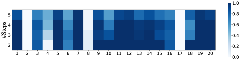
(a) Inconsistent optimal steps.

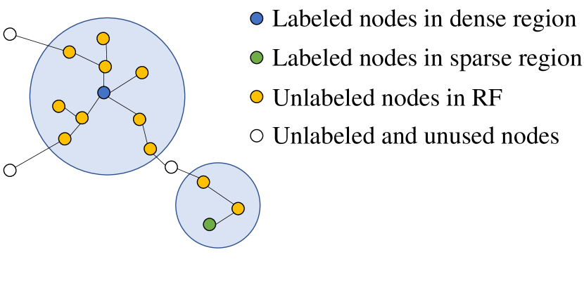
(b) Inconsistent RF expansion speed.

Figure 1. (Left) Test accuracy of SGC on 20 randomly sampled nodes of Citeseer. The X-axis is the node id, and Y-axis is the propagation steps. The color from white to blue represents the ratio of being predicted correctly in 50 different runs. (Right) The node in the dense region has a larger RF within two iterations of propagation.

Lines of simplified GNNs are proposed to tackle the fixed RF issue in SGC. SIGN (Frasca et al., 2020) concatenates all the propagated features without information loss, while S²GC (Zhu and Koniusz, 2021) averages all these propagated features to generate the combined feature. Although multi-scale knowledge is considered, the importance and correlations between different scales are ignored in these methods. To fill this gap, GBP (Chen et al., 2020) adopts a heuristic constant decay factor for the weighted average for propagated features at different propagation steps. Motivated by Personalized PageRank, the features with a larger propagation step has a higher risk of over-smoothing (Li et al., 2018; Xu et al., 2018), and they will contribute less to the combination in GBP.

Unfortunately, the coarse-grained, layer-wise combination prevents these methods from unleashing their full potential. As shown in Fig. 1(a), different nodes require different propagation steps to achieve optimal predictive accuracy. Besides, assigning the same weight distribution to propagated features along with propagation depth to all the nodes may be unsuitable due to the inconsistent RF expansion speed shown in Fig. 1(b). However, nodes in most existing GNNs are restricted to a fixed-hop neighborhood and insensitive to the actual demands of different nodes.

Motivated by the above observations, we propose to explicitly learn the importance and correlation of multi-scale knowledge in a node-adaptive manner. To this end, we develop a new architecture – Graph Attention Multi-Layer Perceptron (GAMLP) – that could automatically exploit the knowledge over different neighborhoods at the granularity of nodes. GAMLP achieves this by introducing two novel attention mechanisms: Recursive attention and Jumping Knowledge (JK) attention. These two attention mechanisms can capture the complex correlations between propagated information at different propagation depths in a node-adaptive manner. Consequently, GAMLP has the same benefits as the existing simplified and scalable GNN models while providing much better performance derived from its ability to utilize a node-adaptive RF. Moreover, the proposed attention mechanisms can be applied to both node features and labels over neighborhoods with different sizes. By combining these two categories of information, GAMLP could achieve the best of both worlds in terms of accuracy.

Our contributions are as follows: (1) New perspective. We propose GAMLP, a scalable, efficient, and deep graph model. To the best of our knowledge, GAMLP is the first to explore both node-adaptive feature and label propagation schemes in scalable GNNs. (2) Real world deployment and applications. We deploy GAMLP in a distributed training manner in Tencent, and it has been widely used to support many applications in the real-world production environment. (3) State-of-the-art performance. Experimental results demonstrate that GAMLP achieves state-of-the-art performance on 14 graph datasets while maintaining high scalability and efficiency. For example, GAMLP outperforms GAT by 1.3% regarding predictive accuracy on our large-scale Tencent Video dataset while achieving up to $50\times$ training speedup. Besides, it outperforms the competitive baseline GraphSAINT (Zeng et al., 2020) in terms of accuracy by a margin of $0.42\%$, $3.02\%$ and $0.44\%$ on PPI, Flickr, and Reddit datasets under the inductive setting. Under the transductive setting in large OGB datasets, the accuracy of GAMLP exceeds the second-best method by $1.03\%$, $1.32\%$ $1.61\%$ on the ogbn-products, ogbn-papers100M, and ogbn-mag datasets, respectively.

2. Preliminaries

2.1. Problem Formulation

We consider an undirected graph $\mathcal{G}$ = ($\mathcal{V}$,$\mathcal{E}$) with $|\mathcal{V}|=n$ nodes, $|\mathcal{E}|=m$ edges, and $c$ different node classes. We denote by $\mathbf{A}$ the adjacency matrix of $\mathcal{G}$, weighted or not. Each node has a feature vector of size $f$, stacked up in an $n\times f$ matrix $\mathbf{X}$. $\mathbf{D}=\operatorname{diag}\left(d_{1},d_{2},\cdots,d_{n}\right)\in\mathbb{R}^{n\times n}$ denotes the degree matrix of $\mathbf{A}$, where $d_{i}=\sum_{v_{j}\in\mathcal{V}}\mathbf{A}_{ij}$ is the degree of node $v_{i}$. Suppose $\mathcal{V}_{l}$ is the labeled set, and our goal is to predict the labels for nodes in the unlabeled set $\mathcal{V}_{u}$ with the supervision of $\mathcal{V}_{l}$.

2.2. Scalable GNNs

Sampling. As a node-wise sampling method, GraphSAGE (Hamilton et al., 2017) randomly samples a fixed-size set of neighbors for computation in each mini-batch. VR-GCN (Chen et al., 2018b) analyzes the variance reduction, and it reduces the size of samples with additional memory cost. For the layer-wise sampling, Fast-GCN (Chen et al., 2018a) samples a fixed number of nodes at each layer, and ASGCN (Huang et al., 2018) proposes the adaptive layer-wise sampling with better variance control. In the graph level, Cluster-GCN (Chiang et al., 2019) firstly clusters the nodes and then samples the nodes in the clusters, and GraphSAINT (Zeng et al., 2020) directly samples a subgraph for mini-batch training. Recently, sampling has already been widely used in many GNNs and GNN systems (Zheng et al., 2020; Zhu et al., 2019; Fey and Lenssen, 2019).

Graph-wise Propagation. Recent studies have observed that non-linear feature transformation contributes little to the performance of the GNNs as compared to feature propagation. Thus, a new direction for scalable GNN is based on the simplified GCN (SGC) (Wu et al., 2019), which successively removes nonlinearities and collapsing weight matrices between consecutive layers. SGC reduces GNNs into a linear model operating on $K$-layers propagated features:

(1) $$\small\mathbf{X}^{(K)}=\mathbf{\hat{A}}^{K}\mathbf{X}^{(0)},\qquad\mathbf{Y}=\text{softmax}(\mathbf{\Theta}\mathbf{X}^{(K)}),$$

where $\mathbf{X}^{(0)}=\mathbf{X}$, $\mathbf{X}^{(K)}$ is the $K$-layers propagated feature, $\mathbf{\hat{A}}=\widetilde{\mathbf{D}}^{r-1}\widetilde{\mathbf{A}}\widetilde{\mathbf{D}}^{-r}$, and $\widetilde{\mathbf{A}}=\mathbf{A}+\mathbf{I}_{N}$ is the adjacency matrix $\mathbf{A}$ with self loops added. $\mathbf{\hat{D}}$ is the corresponding degree matrix of $\mathbf{\hat{A}}$. By setting $r=$ 0.5, 1 and 0, $\mathbf{\hat{A}}$ represents the symmetric normalization adjacency matrix $\widetilde{\mathbf{D}}^{-1/2}\widetilde{\mathbf{A}}\widetilde{\mathbf{D}}^{-1/2}$ (Klicpera et al., 2019), the transition probability matrix $\widetilde{\mathbf{A}}\widetilde{\mathbf{D}}^{-1}$ (Zeng et al., 2020), or the reverse transition probability matrix $\widetilde{\mathbf{D}}^{-1}\widetilde{\mathbf{A}}$ (Xu et al., 2018), respectively. As the propagated features $\mathbf{X}^{(K)}$ can be precomputed, SGC is easy to scale to large graphs. However, graph-wise propagation restricts the same propagation steps and a fixed RF for each node. Therefore, some nodes’ features may be over-smoothed or under-smoothed due to the inconsistent RF expansion speed, leading to non-optimal performance.

Layer-wise Propagation. Following SGC, some recent methods adopt layer-wise propagation to combine the features with different propagation layers. SIGN (Frasca et al., 2020) proposes to concatenate the propagated features at different propagation depth after simple linear transformation: $[\mathbf{X}^{(0)}\mathbf{W}_{0},\mathbf{X}^{(1)}\mathbf{W}_{1},...,\mathbf{X}^{(K)}\mathbf{W}_{K}]$. S²GC (Zhu and Koniusz, 2021) proposes the simple spectral graph convolution to average the propagated features in different iterations as $\mathbf{X}^{(K)}=\sum\limits_{l=0}\limits^{K}\mathbf{\hat{A}}^{l}\mathbf{X}^{(0)}$. In addition, GBP (Chen et al., 2020) further improves the combination process by weighted averaging as $\mathbf{X}^{(K)}=\sum\limits_{l=0}\limits^{K}w_{l}\mathbf{\hat{A}}^{l}\mathbf{X}^{(0)}$ with the layer weight $w_{l}=\beta{(1-\beta)}^{l}$. We also use a linear model for higher training scalability similar to these works. The difference lies in that we consider the propagation process from a node-wise perspective, and each node in GAMLP has a personalized combination of different steps of the propagated features.

2.3. Label Utilization in GNNs.

Labels of training nodes are conventionally only used as supervision signals in loss functions in most graph learning methods. However, there also exist some graph learning methods that directly exploit the labels of training nodes. Among them, the label propagation algorithm (Zhu and Ghahramani, 2002) is the most well-known one. It simply regards the partially observed label matrix $\mathbf{Y}\in\mathbb{R}^{N\times C}$ as input features for nodes in the graph and propagates the input features through the graph structure, where $C$ is the number of candidate classes. UniMP (Shi et al., 2020) proposes to map the partially observed label matrix $\mathbf{Y}$ to the dimension of the node feature matrix $\mathbf{X}$ and add these two matrices together as the new input feature. To fight against the label leakage problem, UniMP further randomly masks the training nodes during every training epoch.

Instead of using the hard training labels, Correct & Smooth (Huang et al., 2020) first trains a simple model (e.g., MLP) and gets the predicted soft labels for unlabeled nodes. Then, it propagates the learning errors on the labeled nodes to connected nodes and smooths the output in a Personalized PageRank manner like APPNP (Klicpera et al., 2019). Besides, SLE (Sun and Wu, 2021) decouples the label utilization procedure in UniMP, and executes the propagation in advance. Unlike UniMP, “label reuse” (Wang et al., 2021a) concatenates the partially observed label matrix $\mathbf{Y}$ with the node feature matrix $\mathbf{X}$ to form the new input matrix. Concretely, it fills the missing elements in the partially observed label matrix $\mathbf{Y}$ with the soft label predicted by the model, and this newly generated $\mathbf{Y}^{\prime}$ is again concatenated with $\mathbf{X}$ and then fed into the model.

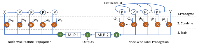
Figure 2. Overview of the proposed GAMLP, including (1) feature and label propagation, (2) combine the propagated features and labels with RF attention, and (3) MLP training. Note that both the feature and label propagation can be pre-processed.

3. Graph Attention Multi-Layer Perceptron

3.1. Architecture Overview

As shown in Fig. 2, GAMLP decomposes the end-to-end GNN training into three parts: feature and label propagation, feature and label combination with RF attention, and the MLP training. As the feature and label propagation is pre-processed only once, and MLP training is efficient and salable, we can easily scale GAMLP to large graphs. Besides, with the RF attention, each node in GAMLP can adaptively get the suitable combination weights for propagated features and labels under different receptive fields, thus boosting model performance.

3.2. Node-wise Feature and Label Propagation

Node-wise Feature Propagation.

We separate the essential operation of GNNs — feature propagation by removing the neural network $\mathbf{\Theta}$ and nonlinear activation $\delta$ for feature transformation. Specifically, we construct a parameter-free $K$-step feature propagation as:

(2) $$\small\mathbf{X}^{(k)}\leftarrow\hat{\mathbf{A}}\mathbf{X}^{(k-1)},\ \forall k=1,\ldots,K,$$

where $\mathbf{X}^{(k)}$ contains the features of a fixed RF: the node itself and its $k$-hop neighborhoods.

After $K$-step feature propagation shown in E.q. 2, we correspondingly get a list of propagated features under different propagation steps: $[\mathbf{X}^{(0)},\mathbf{X}^{(1)},\mathbf{X}^{(k)},...,\mathbf{X}^{(K)}]$. For a node-wise propagation, we propose to average these propagated features in a weighted manner:

(3) $$\small\mathbf{H}_{\mathbf{X}}=\sum_{k=0}^{K}\mathbf{W}_{k}\mathbf{X}^{(k)},$$

where $\mathbf{W}_{k}=Diag(\eta_{k})\in\mathbb{R}^{n\times n}$ is the diagonal matrix derived from vector $\eta_{k}$, and $\eta_{k}\in\mathbb{R}^{n}$ is a vector derived from vector $\eta_{k}[i]=w_{i}(k),1\leq i\leq n$, and $w_{i}(k)$ measures the importance of the $k$-step propagated feature for node $v_{i}$.

Node-wise Label Propagation.

We use a scalable and node-adaptive way to take advantage of the node labels of the training set. Concretely, the label embedding matrix $\mathbf{Y}\in\mathbb{R}^{n\times c}$ ($\mathbf{Y}^{(0)}$) is propagated with the normalized adjacency matrix $\hat{\mathbf{A}}$:

(4) $$\small\mathbf{Y}^{(l)}\leftarrow\hat{\mathbf{A}}\mathbf{Y}^{(l-1)},\ \forall l=1,\ldots,L,$$

After $L$-step label propagation, we get a list of propagated labels under different propagation steps: $[\mathbf{Y}^{(0)},\mathbf{Y}^{(1)},\mathbf{Y}^{(2)},...,\mathbf{Y}^{(L)}]$. Generally, the propagated label $\mathbf{Y}^{(l)}$ is closer to the original label matrix $\mathbf{Y}^{(0)}$ with a smaller propagation step $l$, and thus face a higher risk of data leakage problem if it is directly used as the model input. We propose the last residual connection to adaptively smooth the different steps of propagated labels.

Definition 3.1 (Last Residual Connection).

Given the propagation step $l$, and a list of propagated labels: $[\mathbf{Y}^{(0)},\mathbf{Y}^{(1)},\mathbf{Y}^{(2)},...,\mathbf{Y}^{(L)}]$, we smooth each label $\mathbf{Y}^{(l)}$ with the smoothed label $\mathbf{Y}^{(L)}$:

(5) $$\small\hat{\mathbf{Y}}^{(l)}\leftarrow(1-\alpha_{l})\mathbf{Y}^{(l)}+\alpha_{l}\mathbf{Y}^{(L)},\ l=1,\ldots,L,$$

where $\alpha_{l}=\cos\left(\frac{\pi l}{2L}\right)$ controls the proportion of $\mathbf{Y}^{(L)}$ in the $l$-step propagated label.

Similar to the node-wise feature propagation strategy introduced in Sec. 3.2, we propose to average these propagated labels in a weighted manner as follow:

(6) $$\small\mathbf{H}_{\mathbf{Y}}=\sum_{l=0}^{L}\hat{\mathbf{W}}_{l}\hat{\mathbf{Y}}^{(l)}.$$

3.3. Node-adaptive Attention Mechanisms

To satisfy different RF requirements for each node, we introduce two RF attention mechanisms to get $w_{i}(k)$. Note that these attention mechanisms can be used in both the feature and label propagation, and we introduce them from a feature perspective here. To apply them for node-wise label propagation, we only need to replace the feature $\mathbf{X}_{i}$ in Eq. 7 and Eq. 8 with the label $\mathbf{Y}_{i}$.

Definition 3.2 (Recursive Attention).

At each propagation step $l$, suppose $s\in\mathbb{R}^{d}$ is a learnable parameter vector, we recursively measure the feature information gain compared with the previous combined feature as:

(7) $$\small\widetilde{\mathbf{X}}_{i}^{(l)}=\mathbf{X}_{i}^{(l)}\parallel\sum_{k=0}^{l-1}w_{i}(k)\mathbf{X}_{i}^{(k)},\quad w_{i}(k)={e^{\widetilde{w}_{i}(k)}}/{\sum\limits_{j=0}\limits^{l-1}e^{\widetilde{w}_{i}(j)}},$$

where $\parallel$ means concatenation, and ${\widetilde{w}_{i}(l)}=\delta(\widetilde{\mathbf{X}}_{i}^{(l)}\cdot s)$. As $\widetilde{\mathbf{X}}_{i}^{(l-1)}\in\mathbb{R}^{d}$ combines the graph information under different propagation steps, large proportion of the information in $\widetilde{\mathbf{X}}_{i}^{(l)}$ may have already existed in $\sum_{k=0}^{l-1}w_{i}(k)\mathbf{X}_{i}^{(k)}$, leading to small information gain. A larger $w_{i}(l)$ indicates the feature $\mathbf{X}_{i}^{(l)}$ is more important to the current state of node $v_{i}$ since combining $\widetilde{\mathbf{X}}_{i}^{(l)}$ will introduce higher information gain.

Jumping Knowledge Network (JK-Net) (Xu et al., 2018) adopts layer aggregation to combine the node embeddings of different GCN layers, and thus it can leverage the propagated nodes’ information with different RF. Motivated by JK-Net, we propose to guide the feature combination process with the model prediction trained on all the propagated features. Concretely, GAMLP with JK attention includes two branches: the concatenated JK branch and the attention-based combination branch.

Definition 3.3 (JK Attention).

Given the MLP prediction of the JK branch as $\mathbf{E}_{i}=\text{MLP}(\mathbf{X}_{i}^{(1)}\parallel\mathbf{X}_{i}^{(2)}\parallel...\parallel\mathbf{X}_{i}^{(K)})\in\mathbb{R}^{K\times f}$, the combination weight is defined as:

(8) $$\small\widetilde{\mathbf{X}}_{i}^{(l)}=\mathbf{X}_{i}^{(l)}\parallel\mathbf{E}_{i},\quad{\widetilde{w}_{i}(l)}=\delta(\widetilde{\mathbf{X}}_{i}^{(l)}\cdot s),\quad w_{i}(l)={e^{\widetilde{w}_{i}(l)}}/{\sum\limits_{k=0}\limits^{K}e^{\widetilde{w}_{i}(k)}}.$$

The JK branch aims to create a multi-scale feature representation for each node, which helps the attention mechanism learn the weight $w_{i}(k)$. The learned weights are then fed into the attention-based combination branch to generate each node’s refined attention feature representation. As the training process continues, the attention-based combination branch will gradually emphasize those neighborhood regions that are more helpful to the target nodes. The JK attention can model a broader neighborhood while enhancing correlations, bringing a better feature representation for each node.

3.4. Model Training

Both the combined feature $\mathbf{H}_{\mathbf{X}}$ and label $\mathbf{H}_{\mathbf{Y}}$ are transformed with MLP, and then be added to get the final output embedding:

(9) $$\small\widetilde{\mathbf{H}}=\text{MLP}(\mathbf{H}_{\mathbf{X}})+\beta\text{MLP}(\mathbf{H}_{\mathbf{Y}}),$$

where $\beta$ is a hyper-parameter that measures the importance of the combined label. For example, some graphs have good features but low-quality labels (e.g., label noise or low label rate), and we should decrease $\beta$ so that more attention is paid to the graph features.

We adopt the Cross-Entropy (CE) measurement between the predicted softmax outputs and the one-hot ground-truth label distributions as the objective function:

(10) $$\mathcal{L}_{CE}=-\sum_{i\in\mathcal{V}_{l}}\sum_{j}\mathbf{Y}_{ij}\log(\text{softmax}(\widetilde{\mathbf{H}})_{ij}),$$

where $\mathbf{Y}_{i}$ is the one-hot label indicator vector.

Table 1. Algorithm analysis for existing scalable GNNs. $n$, $m$, $c$, and $f$ are the number of nodes, edges, classes, and feature dimensions, respectively. $b$ is the batch size, and $k$ refers to the number of sampled nodes. $K$ and $L$ corresponds to the number of times we aggregate features and labels, respectively. Besides, $P$ and $Q$ are the number of layers in MLP classifiers trained with features and labels, respectively.

Type	Method	Pre-processing	Training	Memory
Sampling	GraphSAGE	-	$\mathcal{O}(k^{K}nf^{2})$	$\mathcal{O}(bk^{K}f+Kf^{2})$
	FastGCN	-	$\mathcal{O}(kKnf^{2})$	$\mathcal{O}(bkKf+Kf^{2})$
	Cluster-GCN	$\mathcal{O}(m)$	$\mathcal{O}(Pmf+Pnf^{2})$	$\mathcal{O}(bKf+Kf^{2})$
Graph-wise propagation	SGC	$\mathcal{O}(Kmf)$	$\mathcal{O}(nf^{2})$	$\mathcal{O}(bf+f^{2})$
Layer-wise propagation	SIGN	$\mathcal{O}(Kmf)$	$\mathcal{O}(Pnf^{2})$	$\mathcal{O}(bLf+Pf^{2})$
	S2GC	$\mathcal{O}(Kmf)$	$\mathcal{O}(nf^{2})$	$\mathcal{O}(bf+f^{2})$
	GBP	$\mathcal{O}(Knf+K\frac{\sqrt{m\lg{n}}}{\varepsilon})$	$\mathcal{O}(Pnf^{2})$	$\mathcal{O}(bf+Pf^{2})$
Node-wise propagation	GAMLP	$\mathcal{O}(Kmf+Lmc)$	$\mathcal{O}(Pnf^{2}+Qnc^{2})$	$\mathcal{O}(bf+Pf^{2}+Qc^{2})$

3.5. Properties of GAMLP

High Efficiency and Scalability. Compared with the previous GNNs (e.g., GCN and GraphSAGE), our proposed GAMLP only need to do the feature and label propagation only once. Suppose $P$ and $Q$ are the number of layers in MLP trained with feature and labels, and $k$ is the sampled nodes, the time complexity of GAMLP is $\mathcal{O}(Pnf^{2}+Qnc^{2})$, which is smaller than the complexity of GraphSAGE (i.e., $\mathcal{O}(k^{K}nf^{2})$). Besides, it also costs less memory than the sampling-based GNNs, and thus can scale to a larger graph in a single machine. Notably, like other simplified GNNs (i.e., SGC and SIGN), GAMLP can pre-compute the propagated features and labels only once. It does not need to pull the intermediate representation of other nodes during the MLP training. Therefore, it can also be well adapted to the distributed environment.

Deep propagation. With our recursive and JK attention, GAMLP can support large propagation depths without the over-smoothing issue since each node can get the node personalized combination weights for different propagated features and labels according to its demand. Such characteristic is essential for sparse graph, i.e., sparse labels, edges, and features. For example, a graph with a low label rate or edge rate can increase the propagation depth to spread the label supervision over the entire graph. Each node can utilize the high-order graph structure information with deep propagation and boost the node classification performance. Further details are in Appendix B.1.

3.6. Complexity Analysis

Table 1 provides a detailed asymptotic complexity comparison between GAMLP and representative scalable GNN methods. During preprocessing, the time cost of clustering in Cluster-GCN is $\mathcal{O}(m)$ and the time complexity of most linear models is $\mathcal{O}(Kmf)$. Besides, GAMLP has an extra time cost $\mathcal{O}(Lmc)$ for the propagation of training labels. GBP takes advantage of Monte-Carlo method and conducts this process approximately with a bound of $\mathcal{O}(Knf+K\frac{\sqrt{m\lg{n}}}{\varepsilon})$, where $\varepsilon$ is a error threshold. Compared with sampling-based GNNs, graph/layer/node-wise-propagation-based models usually have smaller training and inference time complexity. Memory complexity is a crucial factor in large-scale graph learning as it fundamentally determines whether it is possible to adopt the method. Compared with SIGN, both GBP and GAMLP do not need to store smoothed features at different propagation steps, and the memory complexity can be reduced from $\mathcal{O}(bLf)$ to $\mathcal{O}(bf)$.

4. Experiments

In this section, we verify the effectiveness of GAMLP on 14 real-world graph datasets under (1) both the transductive and inductive settings; and (2) both the homogeneous and heterogeneous graphs. We aim to answer the following five questions. Q1: Can GAMLP outperform the state-of-the-art GNN methods regarding predictive accuracy on real-world datasets? Q2: If GAMLP is effective, where does the performance gain of GAMLP come from? Q3: How does GAMLP perform when applied to highly sparse graphs (i.e., given few edges and low label rate)? Q4: Can GAMLP adapt to and perform well on heterogeneous graphs? More experimental results can be found in Appendix B.

4.1. Experimental Setup

Datasets. We evaluate the performance of GAMLP under both transductive and inductive settings. For transductive settings, we conduct experiments on 11 transductive datasets: three citation network datasets (Cora, Citeseer, PubMed) (Sen et al., 2008), two user-item datasets (Amazon Computer, Amazon Photo), two co-author datasets (Coauthor CS, Coauthor Physics) (Shchur et al., 2018), and three OGB datasets (ogbn-products, ogbn-papers100M, ogbn-mag) (Hu et al., 2021), and one Tencent Video graph. For inductive settings, we perform the comparison experiments on 3 widely used inductive datasets: PPI, Flickr, and Reddit (Zeng et al., 2020). The ogbn-mag dataset is also used to test the ability of GAMLP in a heterogeneous graph. The statistics about these 14 datasets are summarized in Table 11 of Appendix C.1.

Baselines. Under the transductive setting, we compare GAMLP with the following representative baseline methods: GCN (Kipf and Welling, 2016), GAT (Veličković et al., 2017), JK-Net (Xu et al., 2018), ResGCN (Li et al., 2019), APPNP (Klicpera et al., 2019), AP-GCN (Spinelli et al., 2020), UniMP (Shi et al., 2020), SGC (Wu et al., 2019), SIGN (Frasca et al., 2020), S²GC (Zhu and Koniusz, 2021), and GBP (Chen et al., 2020). For the comparison in the OGB datasets, we choose the top-performing methods from the OGB leaderboard along with their accuracy results. Under the inductive setting, we choose following representative methods: SGC (Wu et al., 2019), GraphSAGE (Hamilton et al., 2017), Cluster-GCN (Chiang et al., 2019), and GraphSAINT (Zeng et al., 2020). Besides, for heterogeneous graph, we choose eight baseline methods from the OGB ogbn-mag leaderboard: R-GCN (Schlichtkrull et al., 2018), SIGN (Frasca et al., 2020), HGT (Hu et al., 2020), R-GSN (Wu et al., 2021), HGConv (Yu et al., 2020b), R-HGNN (Yu et al., 2021), and NARS (Yu et al., 2020a).

In addition, two variants of GAMLP are tested in the evaluation: GAMLP(JK) and GAMLP(R). “JK” and “R” stand for adopting “JK attention” and “Recursive attention” for the node-adaptive attention mechanism, respectively. The detailed hyperparameters and experimental environment can be found in Appendix C.2 and Appendix C.1, respectively.

Table 2. Transductive performance on citation networks.

Methods	Cora	Citeseer	PubMed
GCN	81.8$\pm$0.5	70.8$\pm$0.5	79.3$\pm$0.7
GAT	83.0$\pm$0.7	72.5$\pm$0.7	79.0$\pm$0.3
JK-Net	81.8$\pm$0.5	70.7$\pm$0.7	78.8$\pm$0.7
ResGCN	82.2$\pm$0.6	70.8$\pm$0.7	78.3$\pm$0.6
APPNP	83.3$\pm$0.5	71.8$\pm$0.5	80.1$\pm$0.2
AP-GCN	83.4$\pm$0.3	71.3$\pm$0.5	79.7$\pm$0.3
SGC	81.0$\pm$0.2	71.3$\pm$0.5	78.9$\pm$0.5
SIGN	82.1$\pm$0.3	72.4$\pm$0.8	79.5$\pm$0.5
S2GC	82.7$\pm$0.3	73.0$\pm$0.2	79.9$\pm$0.3
GBP	83.9$\pm$0.7	72.9$\pm$0.5	80.6$\pm$0.4
GAMLP(JK)	84.3$\pm$0.8	74.6$\pm$0.4	80.7$\pm$0.4
GAMLP(R)	83.9$\pm$0.6	73.9$\pm$0.6	80.8$\pm$0.5

Table 3. Transductive performance on the co-authorship and co-purchase graphs.

Methods	Amazon Computer	Amazon Photo	Coauthor CS	Coauthor Physics
GCN	82.4$\pm$0.4	91.2$\pm$0.6	90.7$\pm$0.2	92.7$\pm$1.1
GAT	80.1$\pm$0.6	90.8$\pm$1.0	87.4$\pm$0.2	90.2$\pm$1.4
JK-Net	82.0$\pm$0.6	91.9$\pm$0.7	89.5$\pm$0.6	92.5$\pm$0.4
ResGCN	81.1$\pm$0.7	91.3$\pm$0.9	87.9$\pm$0.6	92.2$\pm$1.5
APPNP	81.7$\pm$0.3	91.4$\pm$0.3	92.1$\pm$0.4	92.8$\pm$0.9
AP-GCN	83.7$\pm$0.6	92.1$\pm$0.3	91.6$\pm$0.7	93.1$\pm$0.9
SGC	82.2$\pm$0.9	91.6$\pm$0.7	90.3$\pm$0.5	91.7$\pm$1.1
SIGN	83.1$\pm$0.8	91.7$\pm$0.7	91.9$\pm$0.3	92.8$\pm$0.8
S2GC	83.1$\pm$0.7	91.6$\pm$0.6	91.6$\pm$0.6	93.1$\pm$0.8
GBP	83.5$\pm$0.8	92.1$\pm$0.8	92.3$\pm$0.4	93.3$\pm$0.7
GAMLP(JK)	84.5$\pm$0.7	92.8$\pm$0.7	92.6$\pm$0.5	93.6$\pm$1.0
GAMLP(R)	84.2$\pm$0.5	92.6$\pm$0.8	92.8$\pm$0.7	93.2$\pm$1.0

Table 4. Performance comparison on ogbn-products.

Methods	Val Accuracy	Test Accuracy
GCN	92.00$\pm$0.03	75.64$\pm$0.21
SGC	92.13$\pm$0.02	75.87$\pm$0.14
GraphSAGE	92.24$\pm$0.07	78.50$\pm$0.14
GraphSAINT	92.52$\pm$0.13	80.27$\pm$0.26
GBP	92.82$\pm$0.10	80.48$\pm$0.05
SIGN	92.99$\pm$0.04	80.52$\pm$0.16
DeeperGCN	92.38$\pm$0.09	80.98$\pm$0.20
UniMP	93.08$\pm$0.17	82.56$\pm$0.31
SAGN	93.09$\pm$0.04	81.20$\pm$0.07
SAGN+0-SLE	93.27$\pm$0.04	83.29$\pm$0.18
GAMLP(JK)	93.19$\pm$0.03	83.54$\pm$0.25
GAMLP(R)	93.11$\pm$0.05	83.59$\pm$0.09

Table 5. Performance comparison on ogbn-papers100M.

Methods	Val Accuracy	Test Accuracy
SGC	66.48$\pm$0.20	63.29$\pm$0.19
SIGN	69.32$\pm$0.06	65.68$\pm$0.06
SIGN-XL	69.84$\pm$0.06	66.06$\pm$0.19
SAGN	70.34$\pm$0.99	66.75$\pm$0.84
SAGN+0-SLE	71.06$\pm$0.08	67.55$\pm$0.15
GAMLP(JK)	71.92$\pm$0.04	68.07$\pm$0.10
GAMLP(R)	71.21$\pm$0.03	67.46$\pm$0.02

4.2. End-to-end Comparison

Transductive Performance. To answer Q1, we report the transductive performance of GAMLP in Tables 2, 3 4, and 5. We observe that both variants of GAMLP outperform all the baseline methods on almost all the datasets. For example, on the small Citeseer dataset, GAMLP(JK) outperforms the state-of-the-art method S²GC by a large margin of 1.6%; on the medium-sized Amazon Computers, the predictive accuracy of GAMLP (JK) exceeds the one of the state-of-the-art method GBP by 1.0%; on the two large OGB datasets, GAMLP takes the lead by 1.03% and 1.32% on ogbn-products and ogbn-papers100M, respectively. Furthermore, the experimental results illustrate that the contest between the two variants of GAMLP is not a one-horse race. Thus, these two different attention mechanisms have their irreplaceable sense in some ways.

Table 6. Performance comparison on three inductive datasets.

Methods	PPI	Flickr	Reddit
SGC	65.7$\pm$0.01	50.2$\pm$0.12	94.9$\pm$0.00
GraphSAGE	61.2$\pm$0.05	50.1$\pm$0.13	95.4$\pm$0.01
Cluster-GCN	99.2$\pm$0.04	48.1$\pm$0.05	95.7$\pm$0.00
GraphSAINT	99.4$\pm$0.03	51.1$\pm$0.10	96.6$\pm$0.01
GAMLP(JK)	99.82$\pm$0.01	54.12$\pm$0.01	97.04$\pm$0.01
GAMLP(R)	99.66$\pm$0.01	53.12$\pm$0.00	96.62$\pm$0.01

Inductive Performance. The experiment results in Table 6 show that GAMLP consistently outperforms all the baseline methods under the inductive setting. The leading gap of GAMLP(JK) over SOTA inductive method – GraphSAINT is more than 3.0% on the widely-used dataset – Filckr. The impressive performance of GAMLP under the inductive setting illustrates that GAMLP is powerful in predicting the properties of unseen nodes.

4.3. Ablation Study

To answer Q2, we focus on two modules in GAMLP: (1) label utilization; (2) attention mechanism in the node-wise propagation. For the second one, we evaluate the effects of different choices for reference vectors in the JK attention.

Label Utilization. In this part, we evaluate whether adding the last residual connection and making use of training labels help or not. The predictive accuracy of GAMLP(R) is evaluated on the ogbn-products dataset along with its three variants: “-no_label”, “-plain_label”, and “-uniform”, which stands for not using labels, removing last residual connections, and replacing last residual connections with uniform distributions, respectively. The experimental results in Table 7 show that utilizing labels brings significant performance gain to GAMLP: from 81.43% to 83.59%. The performance drop from removing the last residual connections (“-plain_label” in Table 7) is significant since directly adopting the raw training labels leads to the overfitting issue. The fact that “-uniform” performs worse than “-no_label” illustrates that intuitively fusing the original label distribution with the uniform distribution would harm the predictive accuracy. It further demonstrates the effectiveness of our proposed last residual connections.

Reference Vector in Attention Mechanism. In this part, we study the role of the reference vector (set originally as the concatenated features from different propagation steps) in our proposed JK attention. We evaluate the three variants of GAMLP(JK): “-origin_feature”, “-normal_noise”, and “-no_reference”, which changes the reference vector to the original node feature, noise from the normal distribution, and nothing, respectively. The predictive accuracy of each variant on the PubMed dataset is reported in Table 8. The experimental results show that our original choice of the reference vector is the best among itself and its three variants. The superiority of the concatenated features from different propagation steps comes from the fact that it allows the model to capture the interactions between the propagated features over the receptive fields with different sizes.

Table 7. Ablation study on label utilization.

Methods	Val Accuracy	Test Accuracy
GAMLP(R)	93.11$\pm$0.05	83.59$\pm$0.05
-no_label	92.29$\pm$0.06	81.43$\pm$0.18
-plain_label	92.53$\pm$0.21	81.12$\pm$0.45
-uniform	92.72$\pm$0.15	81.28$\pm$0.93

Table 8. Ablation study on reference vector.

Methods	Val Accuracy	Test Accuracy
GAMLP(JK)	82.5$\pm$0.5	80.7$\pm$0.4
-origin_feature	82.2$\pm$0.4	80.5$\pm$0.4
-normal_noise	81.8$\pm$0.4	79.8$\pm$0.5
-no_reference	81.5$\pm$0.5	79.9$\pm$0.3

Table 9. Test accuracy on ogbn-mag dataset.

Methods	Validation Accuracy	Test Accuracy
R-GCN	40.84$\pm$0.41	39.77$\pm$0.46
SIGN	40.68$\pm$0.10	40.46$\pm$0.12
HGT	49.84$\pm$0.47	49.27$\pm$0.61
R-GSN	51.82$\pm$0.41	50.32$\pm$0.37
HGConv	53.00$\pm$0.18	50.45$\pm$0.17
R-HGNN	53.61$\pm$0.22	52.04$\pm$0.26
NARS	53.72$\pm$0.09	52.40$\pm$0.16
NARS-GAMLP	55.52$\pm$0.08	54.01$\pm$0.21

4.4. Performance on Sparse Graphs

To answer Q3, we conduct experiments to evaluate the predictive accuracy of GAMLP when faced with edge and label sparsity problems, where the number of edges and training labels are highly scarce. We randomly remove a fixed percentage of edges from the original graph to simulate the edge sparsity problem. The removed edges are precisely the same for all the compared methods. Besides, we enumerate the number of training nodes per class from 1 to 20 to evaluate the performance of GAMLP given different levels of label sparsity. The experimental results in Fig. 3 show that GAMLP outperforms all the baselines in most cases when faced with different levels of edge and label sparsity. This experiment further demonstrates the effectiveness of our proposed node-wise propagation scheme. The node-wise propagation enables GAMLP to better capture long-range dependencies, which is crucial when applying GNN methods to highly sparse graphs.

4.5. Performance on Heterogeneous Graphs

Heterogeneous graphs are widely used in many real-world applications. Thus, we measure the performance of GAMLP in heterogeneous graphs and answer Q4. Note that the ogbn-mag dataset only contains node features for “paper” nodes, and we here adopt the ComplEx algorithm (Trouillon et al., 2017) to generate features for other nodes.

Adapting GAMLP to Heterogeneous Graphs. We follow the design of NARS (Yu et al., 2020a) to adapt GAMLP to heterogeneous graphs. First, we sample subgraphs from the original heterogeneous graphs according to the different edge type combinations and regard the sampled subgraph as a homogeneous graph. Then, the propagated features of different steps are generated on each subgraph. The propagated features and labels of the same propagation step across different subgraphs are aggregated using 1-d convolution. After that, aggregated features and labels of different steps are fed into our GAMLP to get the final results. This variant of our GAMLP is called NARS-GAMLP, and we adopt the “JK attention” here.

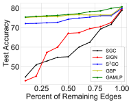
(a) Edge Sparsity

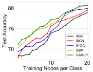
(b) Label Sparsity

Figure 3. Test accuracy on PubMed dataset under different levels of label and edge sparsity.

Experimental Results. We report the validation and test accuracy of our proposed NARS-GAMLP on the ogbn-mag dataset in Table 9. It can be seen from the results that NARS-GAMLP achieves state-of-the-art performance on the heterogeneous graph dataset ogbn-mag. Specifically, it outperforms the strongest single model baseline NARS by a large margin of 1.61% regarding test accuracy.

Table 10. Efficiency and accuracy comparison on the Tencent video classification.

SGC

S2GC

GBP

SIGN

GAMLP(R)

GAMLP (JK)

GCN

APPNP

AP-GCN

JK-Net

ResGCN

GAT

Training Time

1.0

1.2

1.3

3.2

6.1

7.4

33.1

77.8

112.3

112.8

132.3

372.4

Test Accuracy

45.2$\pm$0.3

46.6$\pm$0.6

46.9$\pm$0.7

46.3$\pm$0.5

47.8$\pm$0.4

48.1$\pm$0.6

45.9$\pm$0.4

46.7$\pm$0.6

46.9$\pm$0.7

47.2$\pm$0.3

45.8$\pm$0.5

46.8$\pm$0.7

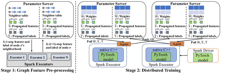
Figure 4. An overview of GAMLP deployed in Tencent.

5. Deployment in Tencent

We now introduce the implementation and deployment of GAMLP in Tencent — the largest social media conglomerate in China.

5.1. GAMLP Training Framework

Unlike most GNNs that entangle the propagation and transformation in the training process, the training of GAMLP is separated into two stages: the graph feature pre-processing and the distributed model training. First, we pre-compute the propagated features and labels with different propagation steps, and then we train the model parameters with the parameter server. Note that both these two stages are implemented in a distributed fashion, and the implementation details of GAMLP can be found in Fig. 4.

Graph feature pre-processing. For the first pre-processing stage, we store the neighbor table, the propagated node features, and labels in a distributed manner. We recursively calculate the propagated features $\overline{\mathbf{X}}=[\mathbf{X}^{(0)},\mathbf{X}^{(1)}...,\mathbf{X}^{(K)}]$ and the propagated labels $\overline{\mathbf{Y}}=[\mathbf{Y}^{(0)},\mathbf{Y}^{(1)}...,\mathbf{Y}^{(L)}]$ for better efficiency. Specifically, to calculate the $i$-th step feature and label for each node $v$ in a batch, we firstly pull the corresponding ($i-1$)-th step feature and label information of its neighbors and then push the propagated feature back to the distributed storage for the calculation of ($i+1$)-th step. The computation of feature and label propagation in each batch is implemented by the Spark executors (Zaharia et al., 2010) in parallel with matrix multiplication. Since we compute the propagated features and labels in parallel, the graph feature pre-processing in the implementation of GAMLP could scale to large graphs and significantly improve the training efficiency in real-world applications.

Distributed training. We implement GAMLP by Angel (Jiang et al., 2020) for the second stage and optimize the parameters with distributed SGD. Specifically, the Spark executors frequently pull the model weights $\overline{\mathbf{W}}$ (including both the attention matrix for weighted average and the parameters of the MLP model), the propagated features $\overline{\mathbf{X}}$ and labels $\overline{\mathbf{Y}}$ from the parameter server. Unlike existing GNN systems (e.g., DistDGL (Zheng et al., 2020) and FlexGraph (Wang et al., 2021b)) that need to sample and pull the neighborhood features in each training epoch, the neighbor table is not used in the training process of GAMLP, and we treat each node as independent and identically distributed. Therefore, the communication cost of training GAMLP can be significantly reduced. Since each spark executor can independently fetches the most up-to-date model weights $\overline{\mathbf{W}}$ and update them in a distributed manner, GAMLP can easily scale to large graphs.

Workflow. The workflow of GAMLP can be summarized as the following steps: 1) The users write the PyTorch scripts and get the PyTorch model. 2) The Spark executor read the PyTorch model and datasets, and pre-computes the propagated features and labels in a distributed manner. 3) The Spark driver pushes the initialized PyTorch model to the parameter server (PS). 4) At each training epoch, every executor samples a batch of nodes and pulls the corresponding model weights, the propagated features, and labels from PS. Then, it updates the model weights with the backpropagation, and pushes the gradients back to PS. Note that we embed PyTorch inside Spark, and we transfer data between JVM runtime and C++ runtime using JNI (Java Native Interface). With our implementation, the users can simply write the python scripts in PyTorch while benefiting from Spark’s distributed data processing.

5.2. Results in WeSee Video Classification

GAMLP has provided service to many applications in Tencent, such as WeSee  short-video classification and WeChat payment prediction. Here we show the effectiveness and efficiency of GAMLP on the short-video classification for the WeSee, a TikTok-like short-video service of Tencent. This task aims to classify short videos into pre-defined 253 classes related to different modalities (such as emotions, theme, place, et al.), which is an important prerequisite for video content understanding and recommendation in WeSee.

Graph construction. We collect 1,000,000 short-videos from the Wesee APP with 57,022 of them manually labeled and then generate a bipartite user-video graph. The edge between each node pair represents that the user has watched (clicked) the short video. Besides, we select 5,000 nodes as the train set, 30,000 nodes as the test set, and an additional validation set of 10,000 labeled nodes for hyper-parameter tuning.

Classification results. Table 10 illustrates the relative training time of each compared method along with its predictive accuracy. The training time of SGC is set to $1.0$ as reference. We observe that (1) The graph/layer-wise propagation-based methods (e.g., SGC and SIGN) have a significant advantage over many widely used GNNs (e.g., GCN and GAT) regarding training efficiency. (2) The two variants of GAMLP achieve the highest predictive accuracy while the training time is acceptable compared to more demanding methods like JK-Net and AP-GCN. The “cold” short videos are less popular, and the corresponding nodes lie in a sparse region of the graph. Thus they need more propagation steps to enhance their node embedding with their distant neighbors. However, simply adopting a large propagation depth will make the propagated node embedding for some “hot” short videos watched by most users indistinguishable. In such cases, the node-wise feature and label propagation of GAMLP are essential to preserving the personalized information of short videos.

6. Conclusion

We present Graph Attention Multilayer Perceptron (GAMLP), a scalable, efficient, and deep graph model based on receptive field attention. GAMLP introduces two new attention mechanisms: recursive attention and JK attention, enabling learning the representations over RF with different sizes in a node-adaptive manner. We have deployed GAMLP in Tencent, and it has served many real-world applications. Extensive experiments on 14 graph datasets verified the high predictive performance of GAMLP. Specifically, in the large-scale short-video dataset from the WeSee APP, the proposed GAMLP exceeded the compared baselines by a large margin in test accuracy while achieving comparable training time with SGC. GAMLP moves forward the performance boundary of scalable GNNs, especially on large-scale and sparse industrial graphs.

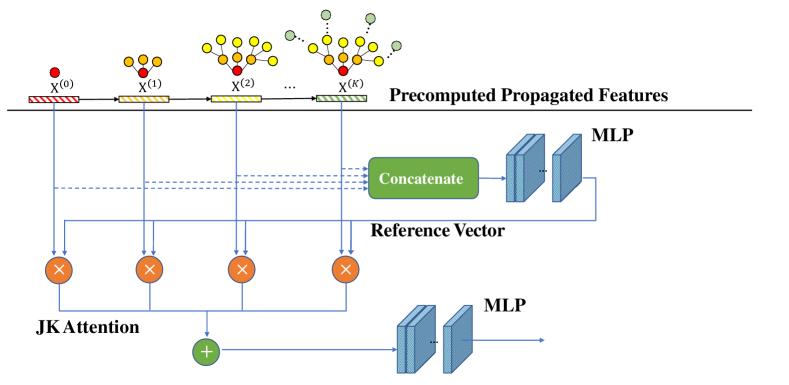
Figure 5. The architecture of GAMLP with JK Attention.

Appendix A More details about GAMLP

A.1. An example of JK attention

Fig. 5 provides a more zoomed-in look of JK attention, one of the two node-adaptive attention mechanisms we proposed. The propagated features are concatenated and then fed into an MLP to map the concatenated feature to the hidden dimension of the model. The mapped feature is then set as the reference vector of the following attention mechanism. A linear layer is adopted to calculate the combination weight for propagated features at different propagation steps. The propagated features are then multiplied with the corresponding combination weight, and the summed results are fed into another MLP to generate final predictions.

A.2. Comparison between the label usage in UniMP and GAMLP

(1) The label usage in UniMP is coupled with the training process, making it hard to scale to large graphs. While GAMLP decouples the label usage from the training process, the label propagation process can be executed as preprocessing.

(2) The label propagation steps in UniMP are restricted to the same number of model layers. Moreover, UniMP will encounter the efficiency and scalability issues even on relatively small graphs if the number of model layers becomes large. In contrast, the label propagation steps in GAMLP can be quite large since the label propagation is performed as preprocessing.

(3) Both propose approaches to fight against the label leakage issue. However, the random masking in UniMP has to be executed in each training epoch, while the last residual connection (composed of simple matrix addition) in GAMLP needs only to be executed once during preprocessing. Thus, UniMP consumes more resources than GAMLP to fight the label leakage issue.

Appendix B Additional experiments

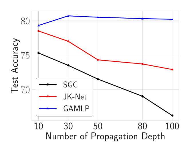
Figure 6. Test accuracy with different propagation depth.

B.1. Deep propagation is possible

Equipped with the learnable node-wise propagation scheme, our GAMLP can still maintain high predictive accuracy even when the propagation depth is over 50. Here, we evaluate the predictive accuracy of our proposed GAMLP(JK) at propagation depth 10, 30, 50, 80, 100 on the PubMed dataset. The performance of JK-Net and SGC are also reported as baselines. The experimental results in Fig. 6 show that even at propagation depth equals 100, the predictive accuracy of our GAMLP(JK) still exceeds 80.0%, higher than the predictive accuracy of most baselines in Table 2. At the same time, the predictive accuracy of SGC and JK-Net both drops rapidly when propagation depth increases from 10 to 100.

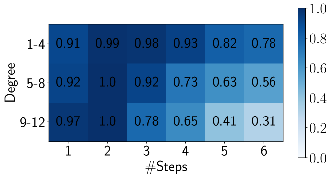
Figure 7. The average attention weights of propagated features of different steps on 60 randomly selected nodes from ogbn-products.

B.2. Interpretability of the attention mechanism

GAMLP can adaptively and effectively combine multi-scale propagated features for each node. To demonstrate this, Fig. 7 shows the average attention weights of propagated features of GAMLP(JK) according to the number of steps and degrees of input nodes, where the maximum step is 6. In this experiment, we randomly select 20 nodes for each degree range (1-4, 5-8, 9-12) and plot the relative weight based on the maximum value. We get two observations from the heat map: 1) The 1-step and 2-step propagated features are always of great importance, which shows that GAMLP captures the local information as those widely 2-layer methods do; 2) The weights of propagated features with larger steps drop faster as the degree grows, indicating that our attention mechanism could prevent high-degree nodes from including excessive irrelevant nodes, leading to over-smoothing. From the two observations, we conclude that GAMLP can identify the different RF demands of nodes and explicitly weight each propagated feature.

Table 11. Overview of the 14 Datasets

Dataset	#Nodes	#Features	#Edges	#Classes	#Train/Val/Test	Task type	Description
Cora	2,708	1,433	5,429	7	140/500/1000	Transductive	citation network
Citeseer	3,327	3,703	4,732	6	120/500/1000	Transductive	citation network
Pubmed	19,717	500	44,338	3	60/500/1000	Transductive	citation network
Amazon Computer	13,381	767	245,778	10	200/300/12881	Transductive	co-purchase graph
Amazon Photo	7,487	745	119,043	8	160/240/7,087	Transductive	co-purchase graph
Coauthor CS	18,333	6,805	81,894	15	300/450/17,583	Transductive	co-authorship graph
Coauthor Physics	34,493	8,415	247,962	5	100/150/34,243	Transductive	co-authorship graph
ogbn-products	2,449,029	100	61,859,140	47	196k/49k/2204k	Transductive	co-purchase graph
ogbn-papers100M	111,059,956	128	1,615,685,872	172	1207k/125k/214k	Transductive	citation network
ogbn-mag	1,939,743	128	21,111,007	349	626k/66k/37k	Transductive	citation network
Tencent Video	1,000,000	64	1,434,382	253	5k/10k/30k	Transductive	user-video graph
PPI	56,944	50	818,716	121	45k / 6k / 6k	Inductive	protein interactions network
Flickr	89,250	500	899,756	7	44k/22k/22k	Inductive	image network
Reddit	232,965	602	11,606,919	41	155k/23k/54k	Inductive	social network

B.3. Choices for $\alpha_{l}$ in Last Residual Connection

Our first choice for the $\alpha_{l}$ in the last residual connection module is $\alpha_{l}=\frac{L-l}{L}$. However, we find that GAMLP still encounters the over-fitting issue on some datasets. Thus, we instead choose $\alpha_{l}=\cos(\frac{\pi l}{2L})$ to give more penalties to labels at large propagation steps. We provide the performance comparison on the ogbn-products dataset in Table 12. Three weighting schemes for the last residual connection module are tested: ”Cosine function” stands for $\alpha_{l}=\cos(\frac{\pi l}{2L})$, the one in GAMLP; ”Linear-decreasing weight” stands for $\alpha_{l}=\frac{L-l}{L}$; and ”Fixed weight” stands for $\alpha_{l}=0.7$. Table 12 shows that the weighting scheme GAMLP adopts, $\alpha_{l}=\cos(\frac{\pi l}{2L})$, outperforms the other two options.

B.4. Efficiency Comparison on ogbn-products

We compare the efficiency of GAMLP with sampling-based GraphSAINT and Cluster-GCN, graph-wise-propagation-based SGC, and layer-wise-propagation-based SIGN on the ogbn-products dataset. The results in Table 13 illustrates that (1) sampling-based methods (e.g., GraphSAINT) consume much more time than graph/layer-wise-propagation based methods (e.g., SGC, SIGN) due to the high computation cost introduced by the sampling process; (2) the two variants of GAMLP achieve the best predictive accuracy while requiring comparable training time with SGC.

Table 12. Ablation study of choices for $\alpha_{l}$ on ogbn-products.

Choices	Test Accuracy
Fixed weight	82.56$\pm$0.43
Linear-decreasing weight	82.72$\pm$0.93
Cosine function	83.59$\pm$0.05

Appendix C Detailed experiment setup

C.1. Experiment Environment

We provide detailed information about the datasets we adopted during the experiment in Table 11. To alleviate the influence of randomness, we repeat each method ten times and report the mean performance and the standard deviations. For the largest ogbn-papers100M dataset, we run each method five times instead. The experiments are conducted on a machine with Intel(R) Xeon(R) Platinum 8255C CPU@2.50GHz, and a single Tesla V100 GPU with 32GB GPU memory. The operating system of the machine is Ubuntu 16.04. As for software versions, we use Python 3.6, Pytorch 1.7.1, and CUDA 10.1. The hyper-parameters in each baseline are set according to the original paper if available. Please refer to Appendix C.2 for the detailed hyperparameter settings for our GAMLP. Besides, the source code of the PyTorch implementation of GAMLP can be found in Github (https://github.com/PKU-DAIR/GAMLP).

C.2. Detailed Hyperparameters

We provide the detailed hyperparameter setting on GAMLP in Table 14, 15 and 16 to help reproduce the results. The hyperparameters are tuned with the toolkit OpenBox (Li et al., 2021) or follow the settings in their original paper. To reproduce the experimental results of GAMLP, just follow the same hyperparameter setting yet only run the python codes.

Table 13. Efficiency comparison on the ogbn-products dataset

. Methods SGC SIGN GAMLP(JK) GAMLP(R) GraphSAINT Cluster-GCN Training time 1.0 4.0 8.0 9.3 364 503 Test accuracy 75.87 80.52 83.54 83.59 79.08 78.97

Table 14. Detailed hyperparameter setting on OGB datasets.

Datasets	attention type	hidden size	num layer in JK	num layer	activation
ogbn-products	Recursive	512	/	4	leaky relu, a=0.2
ogbn-papers100M	JK	1280	4	6	sigmoid
ogbn-mag	JK	512	4	4	leaky relu, a=0.2

Table 15. Detailed hyperparameter setting on OGB datasets.

Datasets	hops	hops for label	input dropout	attention dropout	dropout
ogbn-products	5	10	0.2	0.5	0.5
ogbn-papers100M	12	10	0	0.5	0.5
ogbn-mag	5	3	0.1	0	0.5

Table 16. Detailed hyperparameter setting on OGB datasets.

Datasets	beta	patience	lr	batch size	epochs
ogb-products	1	300	0.001	50000	400
ogb-papers100M	1	60	0.0001	5000	400
ogb-mag	1	100	0.001	10000	400