Long-Term or Temporary?
Hybrid Worker Recruitment for
Mobile Crowd Sensing and Computing

Abstract

Mobile crowd sensing and computing (MCSC) enables heterogeneous users (workers) to contribute real-time sensed, generated, and pre-processed data from their mobile devices to the MCSC platform, for intelligent service provisioning. This paper investigates a novel hybrid worker recruitment problem where the MCSC platform employs workers to serve MCSC tasks with diverse quality requirements and budget constraints, while considering uncertainties in workers’ participation and their local workloads. We propose a hybrid worker recruitment framework consisting of offline and online trading modes. The former enables the platform to overbook long-term workers (services) to cope with dynamic service supply via signing contracts in advance, which is formulated as 0-1 integer linear programming (ILP) with probabilistic constraints related to service quality and budget. Besides, motivated by the existing uncertainties which may render long-term workers fail to meet the service quality requirement of each task, we augment our methodology with an online temporary worker recruitment scheme as a backup Plan B to support seamless service provisioning for MCSC tasks, which also represents a 0-1 ILP problem. To tackle these problems which are proved to be NP-hard, we develop three algorithms, namely, i) exhaustive searching, ii) unique index-based stochastic searching with risk-aware filter constraint, and iii) geometric programming-based successive convex algorithm, which achieve the optimal (with high computational complexity) or sub-optimal (with low complexity) solutions. Experimental results demonstrate the effectiveness of our proposed hybrid worker recruitment mechanism in terms of service quality, time efficiency, etc.

1 Introduction

The past decade has witnessed an enormous increase in the number of intelligent Internet of Things (IoT) devices embedded with powerful processors and sensors, e.g., camera, GPS, gyroscope. This development has led to the rise of a wide range of innovative data- and computation-intensive applications (e.g., traffic information gathering, urban WiFi characterization, weather forecasting, and social services) [1] that aim to process the distributively collected data at the network edge via modern computation techniques [2, 3, 4, 5]. Traditional techniques such as sensor networks have been separately implemented over real-world networks, which, however, may impose high installation cost, suffer from limited spatial coverage, and face difficulties in integrating the distributed mobile computing/storage resources [6].

To this end, Mobile Crowd Sensing and Computing (MCSC) at network edge has been introduced [6, 7]. MCSC represents a novel platform that enables ordinary users to contribute sensed/generated data from their mobile devices, while aggregating and processing heterogeneous crowd sensed data at the network edge for intelligent service provisioning [7, 8], e.g., intelligent urban traffic management. In MCSC platform, IoT devices can act as mobile device clouds (MDCs) [9, 10] equipped with on-board processors and available resources, that pre-process their collected data locally to filtrate useless information, which leads to data redundancy reduction while alleviating the heavy burden of device-to-edge communication and edge server computation processes.

MCSC generally constitutes a three-tiered hierarchical network: i) an edge-based MCSC platform as a centralized controller and data processing center (service requestor), ii) multiple Point-of-Interests (PoIs, a PoI represents a certain region where the MCSC platform is interested in its information and data) coordinated by the edge server, and iii) heterogeneous mobile smart devices (service providers) which are referred to workers. Each PoI can announce various tasks with different service quality requirements (e.g., data quality, pre-processing delay, etc.), while a set of workers around the corresponding PoI are recruited to offer sensing and computing services[11]. Nevertheless, pre-processing a massive amount of collected data on IoT devices and transmitting the corresponding results to the MCSC platform may require individual efforts [11], bringing crucial issues, e.g., extra computation and communication costs. Also, the selfishness of participants (especially workers) [12] may hinder a smooth service provisioning procedure, which calls for proper monetary incentives [6]. These challenges advocate studying MCSC as a service trading market, where the MCSC platform pays commission to each worker according to its contribution to a specific task. To put it succinctly, in this paper, we study trading-empowered MCSC, where during a trading, each recruited worker pre-processes its collected raw data which is required for the successful execution of an MCSC task locally, and transmits the corresponding results to the MCSC platform, while receiving a certain payment.

1.1 Motivations

Existing studies on MCSC have been focused on designing online and offline trading mechanisms for worker recruitment. Online MCSC considers the current information associated with workers and tasks during each practical trading (e.g., information associated with a network snapshot), to conduct online decision-making (e.g., worker-task assignment) [13]. Although online trading can capture the current task/worker/network conditions and achieves relatively accurate decisions, it faces major difficulties to cope with the random and dynamic nature of mobile networks. For example, mobile devices may choose to participate or to be absent from a trading due to i) uncertain mobility, and ii) uncertain dynamic local workloads, which results in dynamic and unwarranted service supply. Furthermore, time-varying wireless network conditions impose uncertainties on the availability of sensing and computing services, e.g., a large data transmission delay can be incurred by poor wireless channel quality between a worker and the gateway of the MCSC platform. Major challenges associated with online MCSC caused by the uncertainties are detailed below:

$\bullet$ Extra latency incurred by online decision-making: Temporal variations of system states (e.g., time-varying channel quality between each worker and the gateway of MCSC platform) require MCSC platform and workers (together referred to participants) to spend excessive amount of time to analyze the current tasks/workers/networks-related information to reach the final agreement during every trading, which reduces the amount of time that can be used for practical sensing and computing. Specifically, since an online decision only works for the current trading, an accumulated latency will be incurred in the long-term upon considering a large number of online trading.

$\bullet$ Extra energy consumption incurred by online decision-making: A long online decision-making procedure can lead to excessive energy consumption, and subsequently a considerable carbon emission and air pollution in long-term [14]. This factor can cause both performance degradation and undesired trading experience, especially in wireless networks with energy-limited mobile devices [2, 15].

$\bullet$ Unexpected trading failures: Online trading may lead to undesired trading failures, and low quality of experience for participants. A typical example is online auctions, where a limited number of winners (winning workers) obtain the eventual employment contracts, while no compensation is offered to the losers (workers who fail in a trading) which also have spent time/energy on bidding/negotiating/waiting. Trading failures can significantly impact the trading experience of participants especially for workers, making them no longer willing to offer services.

We are thus motivated to develop cost-effective and time-efficient service provisioning approaches for MCSC in wireless networks, given the above-mentioned drawbacks of online trading. Offline (in-advance) decision-making offers a feasible solution with less impact on the real-time service delivery [16, 17, 18]. Nevertheless, most of studies on offline trading design for MCSC generally consider known prior information (e.g., prior knowledge of the workers’ locations/resources), which can be impractical to obtain in real-world networks [13, 19].

Given the advantages of online and offline trading modes, this paper introduces a novel hybrid worker recruitment mechanism integrating both offline trading that relies on historical trading statistics [18], and online trading that considers the current worker/task/network conditions. In our developed platform, the offline trading mode determines long-term workers for each task by signing risk-aware contracts in advance, taking into account the historical characteristics of workers/tasks/networks. Long-term workers will offer sensing and computing services to the corresponding tasks during each trading while receiving pre-negotiated payments, without any further negotiation/bargain/bidding with the MCSC platform. This strategy significantly reduces the overhead (e.g., time and energy) of online MCSC decision-making. Specifically, our considered offline trading mode enables the MCSC platform to overbook [21, 22] long-term services from workers, which implies that, the overall service quality promised in pre-signed contracts for a task can be higher than that of its actual demand, given the dynamic service supply. Overbooking helps offering satisfactory quality of service when some long-term workers cannot offer services at some particular trading times, or opt out of a trading [16], e.g., when they are located outside of the corresponding PoI due to their mobility. Although it is important to recruit enough workers for each task, the number of workers is usually constrained by each task’s budget. Thus, the overbooking should be carefully investigated to alleviate the risk of going over budget.

Although overbooking is allowed, the overall service quality offered by long-term workers for a task may be unsatisfying owing to the uncertain workers’ participation and fluctuant quality of service. To this end, we develop an online trading mode as an alternative Plan B to achieve better service quality for MCSC tasks. In the online trading mode, the platform selects temporary workers during each trading when the service requirement (e.g., data quality) of some tasks are not met by long-term workers.

1.2 Relevant Investigations

This paper introduces a novel perspective for multi-tier computing, where heterogeneous workers with different capabilities offer services to MCSC tasks. Correspondingly, we review related works devoted to studying the worker recruitment problem in mobile crowd sensing (MCS), where worker recruitment mechanism is designed while assuming that workers’ information (e.g., sensing qualities) are known in advance [12, 23, 24, 25], which, is impractical in some real-world scenarios.

Recently, few existing works have studied the scenarios with partially unknown information, e.g., unknown sensing qualities and locations of workers. Wang et al. in [13] considered location-aware and location diversity-based dynamic crowd sensing systems with moving workers and stochastic arrival tasks. née Müller et al. [26] introduced a context-aware hierarchical online learning algorithm to maximize the performance of MCS under unknown workers. In [27], Xiao et al. investigated the worker recruitment problem with unknown service qualities, aiming to maximize the total sensing quality under a limited budget, while ensuring workers’ truthfulness and individual rationality. Similarly, Gao et al. in [19] assumed that workers’ sensing qualities and costs are unknown a priori, and focused on continuous sensing tasks. Assuming that sensing quality needs to be protected from disclosure, Zhao et al. in [28] modeled the worker recruitment under unknown service quality as a differentially private multi-armed bandit game. Among existing works, the most relevant work is [11], where Xu et al. designed a pricing scheme which concerns with: the payment offered to the workers, based on their reputations (obtained from historical performance) and their actual performance (during practical trading).

Although the above-mentioned studies have investigated worker recruitment problem from various perspectives, this paper studies this problem from a different angle, as discussed below.

$\bullet$ Trading mode: We introduce a hybrid trading mode where both online and offline trading are exploited, suitable for real-world networks. For example, in our platform, a task can be completed with the help of pre-signed long-term workers; while temporary workers provide backup resources and services. Specifically, this paper encourages overbooking services to each task to cope with the uncertainties, which introduces a novel concept to the literature. Besides, we incorporate soft budget constraints into the mechanism design, where the budget of each task can slightly fluctuate, which is more practical as compared to hard budget assumption that doesn’t allow any changes (e.g,[12]).

$\bullet$ Uncertain factors: We consider various uncertainties in the system, such as unpredictable workers’ participation, mainly due their mobility. Moreover, we analyze the service quality under a more fine-grained representation, in which the local workload of each smart device (worker) is considered. In our considered scenario, each worker can have his own tasks that require multi-dimensional on-board resources, e.g., storage and computing, which can impact the service quality offered to MCSC tasks.

$\bullet$ Risk Evaluation: Since the uncertainties may cause economic losses (e.g., over budget) or unsatisfying services, we evaluate possible risks that both workers and the platform may face, which is neglected in most existing works.

1.3 Challenges

This paper aims to solve the worker recruitment problem for MCSC in wireless networks via considering two stages: i) long-term worker determination (offline mode); and ii) temporary worker recruitment during each trading (online mode). We are facing three key challenges during the first stage:

i) How to determine feasible long-term workers for each task? This is challenging since the service qualities and the participation of workers are unknown prior to each future trading.

ii) How to determine long-term contract terms, such as the payment to a hired worker, and the quality of service that this worker should provide? This is crucial since, on the one hand, tasks can have different budgets and service demands; while, on the other hand, a small payment may lead to negative worker’s utility. This paper considers two levels of quality assurance for each task, namely, hard and soft, to identify the sensing and computing service quality provided by workers.

iii) How to decide the overbooking rate for each task under the service quality requirement and the budget constraint? This is an important aspect of the design since a large overbooking rate can lead to the case where the total payment to long-term workers exceeds the task budget, while a small rate may result in unsatisfying service quality. Although temporary workers can be exploited, online decision-making to recruit them imposes network costs, e.g., latency and energy.

For the second stage (i.e., temporary worker recruitment), the main research question is: How to determine temporary workers for a task when the corresponding long-term workers fail to meet its service quality requirements?

In summary, we solve the fundamental problem of Joint task-to-worker association, as well as payment and service level determination in both online and offline trading modes for MCSC.

1.4 Outlines and Summary of Contributions

This paper considers a three tiered MCSC: an MCSC platform as a service requestor (e.g., edge server), multiple PoIs that can generate tasks with service quality requirements and certain budgets, and multiple workers (e.g., mobile devices) with different capabilities. Also, significant uncertainties are modeled and incorporated into our methodology to better capture the random and unpredictable nature of MCSC networks. For each worker, we consider two levels of service quality: hard and soft quality. The former implies that the worker assigns the highest priority to the scheduled MCSC task, to guarantee a hard service quality assurance by charging a high price. The latter refers to a fluctuating service quality, where the worker will first execute its local workload and then processes the assigned MCSC task, under a lower price. To the best of our knowledge, this work is among the first to study the unknown worker recruitment problem for MCSC networks via considering hybrid trading mode, overbooking, and risk evaluation. Our major contributions are summarized below:

$\bullet$ This paper introduces a novel hybrid worker recruitment mechanism for MCSC via unifying both offline and online trading modes, where uncertain workers’ participation and fluctuant workers’ local workloads are considered to capture the random and unpredictable nature of MCSC.

$\bullet$ The offline worker recruitment mode encourages the MCSC platform to overbook services from long-term workers for each task to cope with the dynamic service supply, by signing employment contracts with payment and service quality level in advance, via analyzing historical statistics associated with uncertainties. Motivated by the existence of uncertainties which may render long-term workers with contracts fail to meet the service quality requirement of each task, we complement our methodology with an online temporary worker recruitment scheme.

$\bullet$ The proposed long-term worker recruitment problem is formulated as a multi-objective optimization (MOO) problem that maximizes the expected utility of the platform and each worker, under acceptable risks (constraints). To tackle the problem, we first develop a methodology based on the state-of-the-art $\epsilon$-constraint method to turn the MOO problem into a single-objective 0-1 integer linear programming (ILP) problem with probabilistic constraints, which is NP-hard. We then design three algorithms to tackle the 0-1 ILP problem: i) exhaustive searching, ii) unique index-based stochastic searching with risk-aware filter constraint, and iii) geometric programming-based successive convex algorithm, which obtain either optimal (with high computational complexity) or sub-optimal (with low computational complexity) solutions. Similar with the above three algorithms associated with offline mode, online mode is considered to select temporary workers to maximize the overall utility of MCSC tasks those with unsatisfying qualities, via analyzing the current network/task/worker conditions.

$\bullet$ Comprehensive simulation results demonstrate that our proposed overbooking-enabled and risk-aware hybrid worker recruitment mechanism for MCSC tasks outperforms baseline methods from different perspectives, e.g., long-term service quality, time efficiency (running time), etc.

The rest of this paper is organized as follows. In Section 2, we provide an overview of MCSC networks and introduce our modeling. Long-term worker determination and contract design problems, as well as temporary worker recruitment problem are proposed and analyzed in Section 3. Experimental results are carried out in Section 4, before drawing the conclusion in Section 5.

2 Overview and System Model

2.1 Overview

We consider an MCSC network consisting of multiple workers gathered via set $\mathbb{W}=\{w_{i}|i\in\{1,2,...,|\mathbb{W}|\}\}$ that can be recruited to collect and compute data for multiple tasks of interest to various PoIs [29, 30] collected via the set $\mathbb{O}=\{{PoI}_{j}|j\in\{1,2,...,|\mathbb{O}|\}\}$. Each ${PoI}_{j}$ periodically generates a certain number of sensing tasks expressed as $\mathbb{S}_{j}=\{\bm{s_{j,k}}|k\in\{1,2,...,|\mathbb{S}_{j}|\}\}$, for the execution of recruited workers through a sequence of trading. During each trading, a worker offers service (namely, contribute and pre-process data) to a task $\bm{s_{j,k}}$ if it stays within the relevant $PoI_{j}$’s region [11, 23, 32] while charging a certain price. We consider two modes for worker recruitment, as detailed below.

i) Offline long-term worker recruitment: This procedure happens in prior to future trading, where the MCSC platform recruits workers for each task via signing long-term contracts in advance, which will be fulfilled accordingly during each trading without any further negotiations. This mode encourages each task to overbook services from workers to cope with the underlying uncertainties in the system. The terms of contract involves a task (namely, a specific task associated with a specific PoI), a worker, the relevant service quality assurance (hard or soft, which will be introduced in Sec. 2.3), as well as the payment. Workers who have signed contracts with the MCSC platform regarding the tasks of ${PoI}_{j}$, are referred to long-term workers of ${PoI}_{j}$.

ii) Online temporary worker recruitment: This procedure occurs during each trading. Due to the dynamics and uncertainties associated with MCSC networks, a task may suffer from the risk of receiving unsatisfying service quality. For example, long-term workers who happen to move outside of the target PoI’s region will fail to provide service to their assigned tasks. To this end, MCSC platform recruits temporary workers without pre-signed contracts for the tasks with unsatisfying service quality, under an online trading mode. Notably, online worker recruitment procedure relies on analyzing the current task/worker/network conditions, which may incur extra latency and energy consumption.

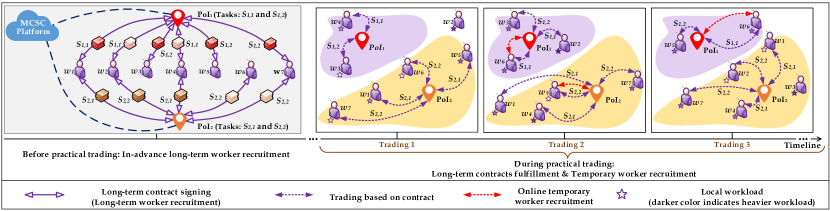
Figure 1: Framework and timeline associated with the proposed hybrid worker recruitment for MCSC in wireless networks. Specifically, the star aside each worker denotes the relevant local workload, where the darker color indicates a heavier local workload that may require more resources (e.g., storage, computing resources, etc.).

Fig. 1 depicts a timeline of our proposed hybrid worker recruitment mechanism, which can be divided into two phases: i) before trading, and ii) during trading. During the former phase, the MCSC platform recruits workers via signing long-term contracts; while in the latter phase, long-term workers and MCSC platform will fulfill their obligations in pre-signed contracts, while some temporary workers may be employed. Also, several practical trading examples are illustrated in Fig. 1, e.g., in trading 1, long-term worker $w_{2}$ fails to serve tasks $\bm{s_{1,1}}$ and $\bm{s_{2,2}}$ since it moves outside of both the two associated PoIs’ coverage zone.

2.2 Task Modeling

We denote task $\bm{s_{j,k}}$ belonging to ${PoI}_{j}$ as a tuple $\bm{s_{j,k}}=\left(d_{j,k}^{B},d_{j,k}^{Q}\right)$, where $d_{j,k}^{B}$ denotes the tolerable budget of the task , which affects the number of employed workers. Also, $d_{j,k}^{Q}$ represents the desired service quality [12], which incorporates the following factors: i) data quality, reliability and accuracy, e.g., high and low-resolution image data can lead to different data qualities; ii) sensing duration, e.g., some workers may need to travel around a certain region for data collection [11, 12, 33]; iii) time for data analyzing (computing), e.g., a worker may have to pre-process the collected raw data locally, to reduce possible data redundancy and heavy computation burden on the MCSC platform; iv) time for uploading data to the MCSC platform through the wireless medium.

2.3 Worker Modeling

We assume that each worker $w_{i}\in\mathbb{W}$ can contribute data and computing service to one task within a PoI region during a trading. To better capture the unpredictable and random nature of MCSC networks, we consider two key uncertainties associated with each worker $w_{i}\in\mathbb{W}$.

$\bullet$ Uncertain participation. This uncertainty describes whether a worker $w_{i}$ is located inside or outside from ${PoI}_{j}$ during a trading process, due to its mobility (in the latter of which it cannot offer sensing and computing service to ${PoI}_{j}$). For worker $w_{i}\in\mathbb{W}$, we let random variable $\alpha_{i}$ denote its attendance in different PoIs’ regions that follows a discrete distribution denoted by $\alpha_{i}\sim\textbf{D}\left\{\left(0,1,...,j,...,|\mathbb{O}|\right),\left(1-\sum_{j=1}^{j=|\mathbb{O}|}a_{i,j},a_{i,1},...a_{i,j},...,a_{i,|\mathbb{O}|}\right)\right\}$, where $0\leqslant\sum_{j=1}^{j=|\mathbb{O}|}a_{i,j}\leqslant 1$. Specifically, $\alpha_{i}=j$ with probability $a_{i,j}$ captures an event in which worker $w_{i}$ is within ${PoI}_{j}$’s coverage; while ${\alpha_{i}=0}$ with probability $1-\sum_{j=1}^{j=|\mathbb{O}|}a_{i,j}$ means that worker $w_{i}$ is absent from the trading (“no show”) [16] since it is located outside of all PoIs’ regions. For notational simplicity, let $\mathbb{A}=\{\alpha_{1},...,\alpha_{i},...,\alpha_{|\mathbb{W}|}\}$ where $\alpha_{i}\in\mathbb{A}$ are independent from each other.

$\bullet$ Uncertain local workload. In practice, workers may also need to handle their local tasks, which can impact the service quality on performing MCSC tasks. For example, a worker’s local tasks may spend a certain period of time for waiting due to the completion of an assigned MCSC task (e.g., wait for the release of occupied computing/storage resources) [17]. The local workload of each worker $w_{i}\in\mathbb{W}$ is modeled by random variable $\beta_{i}$ where $b_{w_{i}}^{-}\leqslant\beta_{i}\leqslant b_{w_{i}}^{+}$, following a normal distribution with mean $\mu_{w_{i}}$ and variance ${(\sigma_{w_{i}})}^{2}$: $\beta_{i}$ obeys a truncated normal distribution [35] $\beta_{i}\sim\textbf{N}\left(\mu_{w_{i}},{(\sigma_{w_{i}})}^{2},b_{w_{i}}^{-},b_{w_{i}}^{+}\right)$. A large value of ${\beta_{i}}$ indicates a heavy local workload that $w_{i}$ needs to handle. For analytical simplicity, let $\mathbb{B}=\{\beta_{1},...,\beta_{i},...,\beta_{|\mathbb{W}|}\}$ where all $\beta_{i}\in\mathbb{B}$ are independent from each other.

2.4 Service Modeling

Participation of a worker in different tasks can incur various costs depending on the complexities and resource requirements of each task [12]. Let $c_{i,j,k}$ denote the cost that $w_{i}$ needs to spend on performing task $\bm{s_{j,k}}$, e.g., energy consumption on collecting/transmitting data or the cost incurred by traveling around the target sensing region. Also, different workers may offer various service qualities of task processing [12, 27, 34], considering factors such as the on-board capabilities of smart devices [12] (e.g., heterogeneous hardware settings), and channel conditions for sensing/data transmission. In addition, the local workload of each worker impacts its service quality. For example, a worker that assigns top priority to its local workload may cause unacceptable MCSC task completion time. Consequently, we consider two quality levels for the services offered by a worker, namely, service with hard quality assurance and service with soft quality assurance detailed below.

$\bullet$ Service with hard quality assurance implies that a worker $w_{i}\in\mathbb{W}$ offers a strict guaranteed service quality $q_{i,j,k,\mathsf{Hard}}$ to task $\bm{s_{j,k}}$, via promising to assign high priority to the assigned MCSC task under any local workload during each trading ($w_{i}$ handles its local tasks after the completion of MCSC task). A worker $w_{i}$ who offers hard service quality assurance may incur a high cost denoted by $r_{i}q_{i,j,k,\mathsf{Hard}}\beta_{i}$, where $r_{i}$ denotes a positive cost factor, where higher required service quality $q_{i,j,k,\mathsf{Hard}}$ and heavier local workload $\beta_{i}$ can incur severe cost on worker $w_{i}$. Let $p_{i,j,k,\mathsf{Hard}}$ indicate the required payment of worker $w_{i}$ for contributing data to task $\bm{s_{j,k}}$ under hard quality assurance.

$\bullet$ Service with soft quality assurance implies that a worker $w_{i}$ will assign high priority to its local tasks, while offering fluctuating service quality to MCSC task $\bm{s_{j,k}}$ during each trading, caused by its uncertain local workload. The soft quality is denoted by $q_{i,j,k,\mathsf{Soft}}=q_{i,j,k,\mathsf{Hard}}-r_{i}^{\prime}\beta_{i}$, where a large value of workload $\beta_{i}$ leads to a low value of $q_{i,j,k,\mathsf{Soft}}$. Specifically, $r_{i}^{\prime}$ measures the marginal performance degradation rate, capturing the performance degradation of MCSC task caused by local workload (e.g., extra processing time for the assigned MCSC task). Let $p_{i,j,k,\mathsf{Soft}}$ denote the required payment of worker $w_{i}$ for providing service to task $\bm{s_{j,k}}$ under soft service quality assurance ($p_{i,j,k,\mathsf{Soft}}<p_{i,j,k,\mathsf{Hard}}$). Although soft assurance may incur risky service quality, it can lead to opportunistic advantages for both parties. For instance, the MCSC platform may enjoy a high service quality at a low price (e.g., considering $\beta_{i}=0$, we have $q_{i,j,k,\mathsf{Soft}}=q_{i,j,k,\mathsf{Hard}}$ and the MCSC platform only pays $p_{i,j,k,\mathsf{Soft}}$). For each $\bm{s_{j,k}}\in\mathbb{S}$, $q_{i,j,k,\mathsf{Soft}}$ also obeys a Truncated normal distribution according to the distribution of $\beta_{i}\in\mathbb{B}$.

3 Proposed Hybrid Worker Recruitment for MCSC

3.1 Long-Term Worker Determination and Contract Design (Offline Mode)

Since all the workers and PoIs are independent from each other, we focus on analyzing the worker recruitment at one PoI and drop the index $j$, without loss of generality (e.g., now we have $\mathbb{S}=\{\bm{s_{k}}|k\in\{1,2,...,|\mathbb{S}|\}\}$, and $\alpha_{i}\sim\textbf{B}\{(0,1),(1-a_{i},a_{i})\}$ where “B” denotes the Bernoulli distribution).

Let $\bm{L}=\{\mathsf{Soft},\mathsf{Hard}\}$ denote the set of quality assurance levels, while $\ell\in\bm{L}$ is the corresponding indicator. Specifically, $x_{i,k,\mathsf{Hard}}=1$, and $x_{i,k,\mathsf{Soft}}=1$ represent that MCSC platform signs a long-term contract with worker $w_{i}$ for sensing task $\bm{s_{k}}$ while offering hard and soft quality assurance, respectively; otherwise $x_{i,k,\mathsf{Hard}}=0$ or $x_{i,k,\mathsf{Soft}}=0$. Also, each worker can be assigned to at most one task under hard or soft quality assurance ($\sum_{\bm{s_{k}}\in\mathbb{S}}\sum_{\ell\in\bm{L}}x_{i,k,\ell}\leqslant 1,\forall w_{i}\in\mathbb{W}$); while a task can recruit multiple workers. We let $\mathbb{Q}=\{q_{i,k,\ell}|w_{i}\in\mathbb{W},\bm{s_{k}}\in\mathbb{S},\ell\in\bm{L}\}$ indicate the service quality profile, $\mathbb{P}=\{p_{i,k,\ell}|w_{i}\in\mathbb{W},\bm{s_{k}}\in\mathbb{S},\ell\in\bm{L}\}$ represent the payment profile, and $\mathbb{X}=\{x_{i,k,\ell}|w_{i}\in\mathbb{W},\bm{s_{k}}\in\mathbb{S},\ell\in\bm{L}\}$ denote the task assignment profile. Fig. 2 illustrates an example of long-term contract signing conducted at a PoI among four workers and two MCSC tasks. In the following, the utility, expected utility, and risk of participants in the offline trading mode are analyzed.

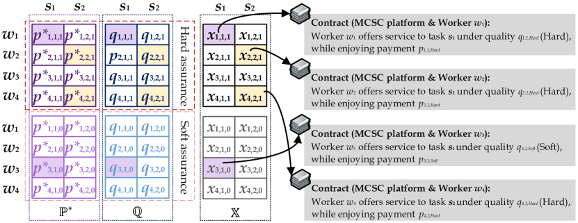
Figure 2: Example of long-term contracts among 4 workers and 2 sensing tasks (the third subscript 1, and 0 denote “Hard”, and “Soft”, respectively for notational simplicity in this figure).

3.1.1 Utility, Expected Utility and Risk

We define the utility of task $\bm{s_{k}}\in\mathbb{S}$ as the overall received service quality, as follows,

$$\mathcal{U}^{s_{k}}\left(\mathbb{X},\mathbb{Q},\mathbb{A}\right)=\sum_{w_{i}\in\mathbb{W}}\alpha_{i}\sum\limits_{\ell\in\bm{L}}x_{i,k,\ell}q_{i,k,\ell},$$ (1)

where $\alpha_{i}$ denotes the participation of worker $w_{i}$, introduced in Sec. 2.3. Correspondingly, the sum utility of all the MCSC tasks is given by

$$\mathcal{U}^{\mathbb{S}}\left(\mathbb{X},\mathbb{Q},\mathbb{A}\right)=\sum_{\bm{s_{k}}\in\mathbb{S}}\sum_{w_{i}\in\mathbb{W}}\alpha_{i}\sum\limits_{\ell\in\bm{L}}x_{i,k,\ell}q_{i,k,\ell}.$$ (2)

Since it is difficult to directly maximize $\mathcal{U}^{\mathbb{S}}\left(\mathbb{X},\mathbb{Q},\mathbb{A}\right)$ due to the unpredictable and random nature of MCSC environment (e.g., uncertain $\alpha_{i}$ and $\beta_{i}$), we focus on the expected value of $\mathcal{U}^{\mathbb{S}}\left(\mathbb{X},\mathbb{Q},\mathbb{A}\right)$, assuming independence between $\alpha_{i}$ and $q_{i,k,\ell}$, $\forall w_{i}\in\mathbb{W},\bm{s_{k}}\in\mathbb{S},\ell\in\bm{L}$, obtained as follows:

$$\overline{\mathcal{U}^{\mathbb{S}}}\left(\mathbb{X},\mathbb{Q},\mathbb{A}\right)=\text{E}\left[\sum_{\bm{s_{k}}\in\mathbb{S}}\sum_{w_{i}\in\mathbb{W}}\alpha_{i}\sum\limits_{\ell\in\bm{L}}x_{i,k,\ell}q_{i,k,\ell}\right]$$

$$=\sum_{\bm{s_{k}}\in\mathbb{S}}\sum_{w_{i}\in\mathbb{W}}a_{i}\sum\limits_{\ell\in\bm{L}}x_{i,k,\ell}\overline{q_{i,k,\ell}},$$ (3)

where $\overline{q_{i,k,\ell}}\triangleq\text{E}\left[q_{i,k,\ell}\right]$ denotes the expected value of service quality. For hard quality assurance, we have $\overline{q_{i,k,\mathsf{Hard}}}=q_{i,k,\mathsf{Hard}}$. Also, given the distribution of $\beta_{i}\in\mathbb{B}$, $q_{i,k,\mathsf{Soft}}$ is a bounded random variable $\mathbbm{q}_{i,k,\mathsf{Soft}}^{-}\leqslant q_{i,k,\mathsf{Soft}}\leqslant\mathbbm{q}_{i,k,\mathsf{Soft}}^{+}$, following a normal distribution with mean $\mu_{q_{i,k,\mathsf{Soft}}}=-r_{i}^{\prime}\mu_{w_{i}}+q_{i,k,\mathsf{Hard}}$ and variance ${\left(\sigma_{q_{i,k,\mathsf{Soft}}}\right)}^{2}={\left(r_{i}^{\prime}\sigma_{w_{i}}\right)}^{2}$, where $\mathbbm{q}_{i,k,\mathsf{Soft}}^{-}=-r_{i}^{\prime}b_{w_{i}}^{+}+q_{i,k,\mathsf{Hard}}$ and $\mathbbm{q}_{i,k,\mathsf{Soft}}^{+}=-r_{i}^{\prime}b_{w_{i}}^{-}+q_{i,k,\mathsf{Hard}}$ are the lower and upper bound of $q_{i,k,\mathsf{Soft}}$, respectively. The expectation of $q_{i,k,\mathsf{Soft}}$ can be calculated as follows

$$\overline{q_{i,k,\mathsf{Soft}}}=\mu_{q_{i,k,\mathsf{Soft}}}$$

$$+\sigma_{q_{i,k,\mathsf{Soft}}}\frac{\phi\left(\frac{\mathbbm{q}_{i,k,\mathsf{Soft}}^{-}-\mu_{q_{i,k,\mathsf{Soft}}}}{\sigma_{q_{i,k,\mathsf{Soft}}}}\right)-\phi\left(\frac{\mathbbm{q}_{i,k,\mathsf{Soft}}^{+}-\mu_{q_{i,k,\mathsf{Soft}}}}{\sigma_{q_{i,k,\mathsf{Soft}}}}\right)}{\Phi\left(\frac{\mathbbm{q}_{i,k,\mathsf{Soft}}^{+}-\mu_{q_{i,k,\mathsf{Soft}}}}{\sigma_{q_{i,k,\mathsf{Soft}}}}\right)-\Phi\left(\frac{\mathbbm{q}_{i,k,\mathsf{Soft}}^{-}-\mu_{q_{i,k,\mathsf{Soft}}}}{\sigma_{q_{i,k,\mathsf{Soft}}}}\right)},$$ (4)

where $\phi()$ and $\Phi()$ indicate the probability density function (PDF), and cumulative distribution function (CDF) of standard normal distribution.

Since long-term employment contracts are signed among the MCSC platform and feasible workers in advance to the future practical trading, potential risks should be carefully considered when designing the corresponding contracts. Specifically, for task $\bm{s_{k}}\in\mathbb{S}$, we consider two major risks as detailed below.

$\bullet$Risk of unsatisfying service quality. Each task is facing the risk of receiving an unsatisfying service quality, mainly due to possible “no show” of long-term workers. We formulate this risk as the probability of obtaining a service quality less than $d_{k}^{Q}$:

$$\mathcal{R}_{1}^{s_{k}}\left(\mathbb{X},\mathbb{Q},\mathbb{A}\right)=\operatorname{Pr}\left\{\frac{\sum\limits_{w_{i}\in\mathbb{W}}\sum\limits_{\ell\in\bm{L}}\alpha_{i}x_{i,k,\ell}q_{i,k,\ell}}{d_{k}^{Q}}\leqslant\lambda_{1}^{s_{k}}\right\},$$ (5)

where $\lambda_{1}^{s_{k}}$ denotes a positive threshold coefficient. In (5), a larger value of $\mathcal{R}_{1}^{s_{k}}$ indicates a higher risk of receiving unsatisfying quality for task $\bm{s_{k}}$.

$\bullet$ Over-budget risk. The existing uncertainties (e.g., in the value of $\alpha_{i}$ and $\beta_{i}$) call for overbooking workers to complete MCSC tasks [12] under desired service qualities. For example, in a trading process, “no show” of the long-term workers may lead to unsuccessful execution of a task. Nevertheless, tasks are generally constrained by their budgets, limiting the number of employed workers. As a result, each task $\bm{s_{k}}\in\mathbb{S}$ is risking overpaying to workers, caused by overbooking. Thus, we formulate the over-budget risk of $\bm{s_{k}}$ as the probability of the payment to the employed workers exceeding the pre-determined budget $d_{k}^{B}$:

$$\mathcal{R}_{2}^{s_{k}}\left(\mathbb{X},\mathbb{P},\mathbb{A}\right)=\operatorname{Pr}\left\{\frac{\sum\limits_{w_{i}\in\mathbb{W}}\sum\limits_{\ell\in\bm{L}}\alpha_{i}x_{i,k,\ell}p_{i,k,\ell}}{d_{k}^{B}}>\lambda_{2}^{s_{k}}\right\},$$ (6)

where $\lambda_{2}^{s_{k}}\geqslant 1$ represents a positive threshold coefficient.

We then define the utility of worker $w_{i}\in\mathbb{W}$ during each trading as the net profit for offering sensing and computing service to the assigned MCSC task:

$$\mathcal{U}^{w_{i}}\left(\mathbb{X},\mathbb{Q},\mathbb{P},\alpha_{i},\beta_{i}\right)$$

$$=\alpha_{i}\sum_{\bm{s_{k}}\in\mathbb{S}}x_{i,k,\mathsf{Hard}}(p_{i,k,\mathsf{Hard}}-c_{i,k}\xi_{i}r_{i}q_{i,k,\mathsf{Hard}}\beta_{i})$$

$$+\alpha_{i}\sum_{\bm{s_{k}}\in\mathbb{S}}x_{i,k,\mathsf{Soft}}(p_{i,k,\mathsf{Soft}}-c_{i,k}),$$ (7)

where $\xi_{i}$ denotes the weight coefficient, and $r_{i}q_{i,k,\mathsf{Hard}}\beta_{i}$ represents the extra local cost incurred by performing task $\bm{s_{k}}$ with high priority. Maximizing (7) directly is challenging due to the uncertainties, thus, we focus on the expected utility of $w_{i}$ given by

$$\overline{\mathcal{U}^{w_{i}}}\left(\mathbb{X},\mathbb{Q},\mathbb{P},\alpha_{i},\beta_{i}\right)$$

$$=a_{i}\sum_{\bm{s_{k}}\in\mathbb{S}}x_{i,k,\mathsf{Hard}}(p_{i,k,\mathsf{Hard}}-c_{i,k})$$

$$-\xi_{i}a_{i}r_{i}\sum_{\bm{s_{k}}\in\mathbb{S}}x_{i,k,\mathsf{Hard}}q_{i,k,\mathsf{Hard}}\overline{\beta_{i}}$$

$$+a_{i}\sum_{\bm{s_{k}}\in\mathbb{S}}(x_{i,k,\mathsf{Soft}}(p_{i,k,\mathsf{Soft}}-c_{i,k})),$$ (8)

where $\overline{\beta_{i}}\triangleq\text{E}[\beta_{i}]=\mu_{w_{i}}+\sigma_{w_{i}}\frac{\phi\left(\mathbbm{b}^{-}_{w_{i}}\right)-\phi\left(\mathbbm{b}^{+}_{w_{i}}\right)}{\Phi\left(\mathbbm{b}^{+}_{w_{i}}\right)-\Phi\left(\mathbbm{b}^{-}_{w_{i}}\right)}$, $\mathbbm{b}^{+}_{w_{i}}=\frac{b^{+}_{w_{i}}-\mu_{w_{i}}}{\sigma_{w_{i}}}$ and $\mathbbm{b}^{-}_{w_{i}}=\frac{b^{-}_{w_{i}}-\mu_{w_{i}}}{\sigma_{w_{i}}}$.

On the other hand, each worker $w_{i}\in\mathbb{W}$ faces the risk of receiving negative utility due to its dynamic local workload. We formulate this risk as the probability of $w_{i}$’s utility being less than the acceptable minimum value $\mathcal{U}^{min}>0$ when participating in the trading as follows:

$$\mathcal{R}^{w_{i}}\left(\mathbb{X},\mathbb{Q},\mathbb{P},\beta_{i}\right)=\text{Pr}\left\{\frac{\mathcal{U}^{w_{i}}\left(\mathbb{X},\mathbb{Q},\mathbb{P},\alpha_{i},\beta_{i}\right)}{\alpha_{i}\mathcal{U}^{min}}\leqslant\lambda_{1}^{w_{i}}\right\}.$$ (9)

3.1.2 Problem Design

Problem Formulation. The long-term worker recruitment problem aims to design feasible long-term contracts, each of which containing: i) task-worker execution configuration, (i.e., $x_{i,k,\ell}$, $\forall w_{i}\in\mathbb{W},\bm{s_{k}}\in\mathbb{S},\ell\in\bm{L}$), ii) service quality level (i.e., hard or soft), and iii) the corresponding payment $p_{i,k,\ell}$, $\forall w_{i}\in\mathbb{W},\bm{s_{k}}\in\mathbb{S},\ell\in\bm{L}$). We formulate this problem as a multi-objective optimization (MOO) given in $\bm{\mathcal{P}_{1}}$, aiming to maximize the overall expected utility of the MCSC platform (i.e., the expected value of the sum service quality of tasks), as shown by (10a), and each worker, as given in (10b).

$$\hskip 14.22636pt\bm{\mathcal{P}_{1}:} \begin{cases}\max\limits_{\mathbb{X}}~{}\overline{\mathcal{U}^{\mathbb{S}}}\left(\mathbb{X},\mathbb{Q},\mathbb{A}\right)\hskip 109.54327pt\text{(10a)}\\ \max\limits_{\mathbb{P}}~{}\overline{\mathcal{U}^{w_{i}}}\left(\mathbb{X},\mathbb{Q},\mathbb{P},\alpha_{i},\beta_{i}\right),\forall w_{i}\in\mathbb{W}\hskip 35.56593pt\text{(10b)}\end{cases}$$

s.t.

$$\text{(C1)}:{\mathcal{R}}_{1}^{s_{k}}\left(\mathbb{X},\mathbb{Q},\mathbb{A}\right)\leqslant{\lambda}_{3}^{s_{k}},\forall\bm{s_{k}}\in\mathbb{S}$$

$$\text{(C2)}:{\mathcal{R}}_{2}^{s_{k}}\left(\mathbb{X},\mathbb{P},\mathbb{A}\right)\leqslant{\lambda}_{4}^{s_{k}},\forall\bm{s_{k}}\in\mathbb{S}$$

$$\text{(C3)}:{\mathcal{R}}^{w_{i}}\left(\mathbb{X},\mathbb{Q},\mathbb{P},\beta_{i}\right)\leqslant{\lambda}_{2}^{w_{i}},\forall w_{i}\in\mathbb{W}$$

$$\text{(C4)}:x_{i,k,\ell}\in\{0,1\},\forall w_{i}\in\mathbb{W},\bm{s_{k}}\in\mathbb{S},\ell\in\bm{L}$$

$$\text{(C5)}:\sum_{\bm{s_{k}}\in\mathbb{S}}\sum_{\ell\in\bm{L}}x_{i,k,\ell}\leqslant 1,\forall w_{i}\in\mathbb{W}.$$

In $\bm{\mathcal{P}_{1}}$, $\lambda_{3}^{s_{k}}$, $\lambda_{4}^{s_{k}}$, and $\lambda_{2}^{w_{i}}$ are threshold coefficients within interval $(0,1]$. Also, (C1) determines the acceptable risk of MCSC platform on receiving unsatisfying service quality; (C2) controls the tolerable soft budget constraint associated with each sensing task; (C3) considers workers’ individual rationality, and aims to keep the risk of having unsatisfied workers within a limit. Further, (C4) and (C5) ensure a feasible worker recruitment and task assignment: a worker can at most serve one MCSC task during a trading.

Problem Transformation. Each objective in the above-mentioned MOO problem involves solving a challenging mixed integer linear programming (MILP) problem, to optimize both continuous (e.g., payment associated with different workers $p_{i,k,\ell}$) and discrete (e.g., task assignment $x_{i,k,\ell}$) variables. Also, $\overline{\mathcal{U}^{w_{i}}}(\mathbb{X},\mathbb{Q},\mathbb{P},\alpha_{i},\beta_{i})$ formalized in (8) is a monotone increasing function with respect to $p_{i,k,\ell}$, associating a high price to a higher utility of each worker. Consequently, we reformulate $\bm{\mathcal{P}_{1}}$ as the following problem $\bm{\mathcal{P}_{2}}$ via utilizing the state-of-the-art $\epsilon-constraint$ method [36], which turns (10b) into constraint (C6) below while keeping (10a) as the main objective:

$$\qquad\qquad\bm{\mathcal{P}_{2}:}\max\limits_{\mathbb{X}}~{}\overline{\mathcal{U}^{\mathbb{S}}}\left(\mathbb{X},\mathbb{Q},\mathbb{A}\right)$$ (11)

s.t.(C1), (C2), (C3), (C4), (C5)

$$\text{(C6)}:\overline{\mathcal{U}^{w_{i}}}(\mathbb{X},\mathbb{Q},\mathbb{P},\alpha_{i},\beta_{i})>0,\forall w_{i}\in\mathbb{W}.$$

Generally, MCSC platform is selfish and prefers to hire workers with lower payments. As a result, MCSC platform can offer a payment slightly higher than what a worker requires, to maximize its utility (as long as each worker get positive utility). Subsequently, constraints (C3) and (C6) can be collectively turned into a fixed payment profile $\mathbb{P}^{*}=\{p_{i,k,\ell}^{*}|w_{i}\in\mathbb{W},\bm{s_{k}}\in\mathbb{S},\ell\in\bm{L}\}$, where each element (i.e., $p_{i,k,\mathsf{Hard}}^{*}$ or $p_{i,k,\mathsf{Soft}}^{*}$) indicates the acceptable payment of each worker under hard/soft quality assurance (that describes why (C6) can be automatically satisfied in $\bm{\mathcal{P}_{3}}$ by applying $\mathbb{P}^{*}$, the derivation of which is detailed in Appendix A). Correspondingly, we rewrite problem $\bm{\mathcal{P}_{2}}$ as $\bm{\mathcal{P}_{3}}$, where (C2) is transformed into (C7):

$$\qquad\quad\bm{\mathcal{P}_{3}:}\max\limits_{\mathbb{X}}~{}\overline{\mathcal{U}^{\mathbb{S}}}\left(\mathbb{X},\mathbb{Q},\mathbb{A}\right)$$ (12)

s.t.(C1), (C4), (C5)

$$\text{(C7)}:\mathcal{R}_{2}^{s_{k}}(\mathbb{X},\mathbb{P}^{*},\mathbb{A})\leqslant\lambda_{4}^{s_{k}},\forall\bm{s_{k}}\in\mathbb{S}.$$

Note that the operation of transferring $\bm{\mathcal{P}_{1}}$ to $\bm{\mathcal{P}_{2}}$, and further to $\bm{\mathcal{P}_{3}}$ is reasonable in real-life networks since the MCSC platform generally dominates the worker recruitment procedure. Namely, it is always the employer (MCSC platform) who determines which worker to hire, as long as meeting the payment required by each worker (e.g., constraints (C3) and (C6)).

Challenges in Solving the Problem. Solving problem $\bm{\mathcal{P}_{3}}$ is non-trivial since it is a 0-1 integer linear programming (ILP) problem which is NP-hard. Furthermore, the constraints of $\bm{\mathcal{P}_{3}}$ are non-trivial to satisfy: each of (C1) and (C7) each contains $|\mathbb{S}|$ probabilistic inequalities. Besides, elements in $\mathbb{X}$ are inter-inhibitive with each other (e.g., constraint (C5) indicates that if $x_{i,k,\mathsf{Hard}}=1$, then $x_{i,k,\mathsf{Soft}}$ should be 0), which further poses significant complications during solution design.

To tackle $\bm{\mathcal{P}_{3}}$, we first introduce an exhaustive searching algorithm (ESA) which obtains the optimal solution of $\bm{\mathcal{P}_{3}}$ and is effective for small problem sizes (e.g., few tasks and workers). Then, inspired by the state-of-the-art implicit enumeration method, we propose a sub-optimal algorithm named unique index-based stochastic searching with risk-aware filter constraint (UISRFC), to overcome the high computational complexity of ESA. Although UISRFC can handle large size problems (e.g., large number of tasks and workers), its performance is strictly constrained by the number of performed iterations and the randomness of stochastic searching, which offers no optimality guarantee. For example, few iterations may lead to the failure for obtaining a good solution, while a large number of iteration will definitely raise the running time. Thus, since $\bm{\mathcal{P}_{3}}$ is highly non-convex, we take one step further and transform this problem into a more mathematically tractable form to achieve better universality in various problem sizes, and develop a geometric programming-based successive convex algorithm (GP-SCA) to solve it. Although it may involve a series of approximations and computations at the MCSC level, it works well for diverse problem sizes.

3.1.3 Design of ESA

ESA is an exhaustive search method over the solution space, the psudo-code of which is given in Alg. 1. In Alg. 1, $\bm{\mathcal{X}_{n}}$ denotes $n$-th solution obtained for $\mathbb{X}$, where $n\in\left\{0,1,2,...,2^{|\mathbb{S}|\times|\mathbb{W}|\times 2}-1\right\}$ indicates the index of solutions. Line 3 shows that each index will be mapped to the corresponding binary number. For example, considering $|\mathbb{S}|=2$, $|\mathbb{W}|=3$, the index $n=5$ can be transferred to a binary number 000000000101, with length $2\times 3\times 2=12$. Although ESA is simple to implement and can reach the optimal solution of $\bm{\mathcal{P}_{3}}$, it suffers from high computational complexity of $\mathcal{O}\left(2^{|\mathbb{S}|\times|\mathbb{W}|\times 2}\right)$, which grows exponentially with respect to the value of $|\mathbb{W}|$ and $|\mathbb{S}|$. This makes this algorithm impractical for large problem sizes (e.g., large number of tasks and workers). Motivated by this, we propose UISRFC in the following.

Input : $\mathbb{S}$, $\mathbb{W}$, $\mathbb{A}$, $\mathbb{B}$, $\mathbb{Q}$, $\mathbb{P}^{*}$

Output : The optimal solution profile $\mathbb{X}^{*}$

1 Initialization: $\bm{\mathcal{X}_{0}}\leftarrow\emptyset$, $u_{0}\leftarrow 0$, $n\leftarrow 0$,

2for $1\leqslant n\leqslant 2^{|\mathbb{S}|\times|\mathbb{W}|\times 2}-1$ do

3      

4      $\bm{\mathcal{X}_{n}}\leftarrow\text{Decimal-to-Binary}(n)$, % Map index $n$ to the corresponding binary number of length $|\mathbb{S}|\times|\mathbb{W}|\times 2$, and transfer the binary number to the solution set $\bm{\mathcal{X}_{n}}$

5      if $\bm{\mathcal{X}_{n}}$ meets constraints (C1), (C5), and (C7) then

6            

7            $u_{n}\leftarrow\overline{\mathcal{U}^{\mathbb{S}}}\left(\bm{\mathcal{X}_{n}},\mathbb{Q},\mathbb{A}\right)$

8            if $u_{n}<u_{n-1}$ then

9                   $u_{n}\leftarrow u_{n-1}$

10                  $\bm{\mathcal{X}_{n}}\leftarrow\bm{\mathcal{X}_{n-1}}$

11            

12      $n\leftarrow n+1$

13$\mathbb{X}^{*}\leftarrow\bm{\mathcal{X}_{n}}$

14end algorithm

Algorithm 1 Exhaustive searching algorithm (ESA)

3.1.4 Design of UISRFC

Given the discrete nature of the problem, obtaining feasible solutions for $\bm{\mathcal{P}_{3}}$ (i.e., $\mathbb{X}$) is one of the most significant difficulties. To this end, inspired by the state-of-the-art implicit enumeration method [38], which is a special case of branch-and-bound method, we propose UISRFC algorithm to alleviate the unapplicable computational complexity of ESA, while achieving commendable solutions for $\bm{\mathcal{P}_{3}}$.

The pseudo-code of UISRFC is given in Alg. 2. UISRFC is an iterative method, where, in each iteration $m$, it first stochastically chooses an index which corresponds to a unique binary number (line 4), and check if it is a feasible solution (lines 5-6). If not, it deletes the index from index set $\bm{N}$ (to achieve unique index property while thus proving time efficiency), and starts another iteration (lines 8-10); if yes, it considers the filter constraints and checks whether they should be updated (lines 11-18). For example, UISRFC updates the lower bound of filter constraint ${\text{(C}}^{f}\text{)}$ every time when $\bm{\mathcal{X}_{n}}$ attains a larger value of (3), as shown in line 13. Based on which, any possible solution that fails to meet ${\text{(C}}^{f}\text{)}$ will be directly abandoned, without considering other constraints. Furthermore, the upper bound of constraint (C7) should also be adjusted every time a lower over-budget risk has been reached, as given by line 18. Specifically, the update of constraints ${\text{(C}}^{f}\text{)}$ and (C7) indicates that a better MCSC platforms’ utility while a lower risk can be achieved by solution $\bm{\mathcal{X}_{n}}$, while solution $\bm{\mathcal{X}_{n+1}}$ in the following iteration should be better than $\bm{\mathcal{X}_{n}}$; otherwise, it will be dropped directly (lines 9-10). With the above-mentioned operations, UISRFC will finally converge in the direction of larger utility and lower risk.

Specifically, the computational complexity of UISRFC relies on the number of iterations, as denoted by $\mathcal{O}\left(M\right)$, where $1\leqslant M\leqslant 2^{|\mathbb{S}|\times|\mathbb{W}|\times 2}$. Thus, UISRFC may suffer from performance degradation under a small number of iteration (e.g., it may fail to find a good solution of $\bm{\mathcal{P}_{3}}$ due to the property of randomness during stochastic searching), upon considering increasing optimization problem sizes. Besides, raising the number of iterations will definitely result in higher running time. For example, considering 100 tasks and 300 workers (namely, $|\mathbb{S}|=100$, $|\mathbb{W}|=300$), there are $2^{100\times 300\times 2}$ potential solutions (although many of them are infeasible) which pose challenges in determining the value of $M$. Also, the operation of stochastic searching of UISRFC brings difficulties in offering optimality guarantee. Therefore, we propose GP-SCA to achieve a trackable version of the optimization problem in the following section.

Input : $\mathbb{S}$, $\mathbb{W}$, $\mathbb{A}$, $\mathbb{B}$, $\mathbb{Q}$, $\mathbb{P}^{*}$

Output : The optimal solution profile $\mathbb{X}^{*}$

1 Initialization: $\bm{N}\leftarrow\{0,1,2,...,2^{|\mathbb{S}|\times|\mathbb{W}|\times 2}-1\}$; $\bm{\mathcal{X}_{n}}\leftarrow\emptyset,\forall n\in\bm{N}$; Iteration $m\leftarrow 1$; $u^{*}\leftarrow 0$; $r^{*}\leftarrow\lambda_{4}^{s_{k}}$; Filter constraint associated with utility ${\text{(C}}^{f}\text{)}:u_{n}\geqslant u^{*}$

2for $m\leqslant M$ do

3      

4      for $\bm{N}\neq\emptyset$ do

5             Randomly choose an index $n$ from set $\bm{N}$

6            $\bm{\mathcal{X}_{n}}\leftarrow\text{Decimal-to-Binary}(n)$, % Map index $n$ to the corresponding binary number of length $|\mathbb{S}|\times|\mathbb{W}|\times 2$; and transfer the binary number to the solution set $\bm{\mathcal{X}_{n}}$

7            if $\bm{\mathcal{X}_{n}}$ meets constraint (C5) then

8                  

9                  $u_{n}\leftarrow\overline{\mathcal{U}^{\mathbb{S}}}\left(\bm{\mathcal{X}_{n}},\mathbb{Q},\mathbb{A}\right)$

10                  else

11                         $\bm{N}\leftarrow\bm{N}/\{n\}$

12                        Go to line 20

13                  

14            

15            if ${\text{(C}}^{f}\text{)}$ is satisfied then

16                  

17                  if $\bm{\mathcal{X}_{n}}$ meets constraints (C1), (C7) then

18                         $u^{*}\leftarrow u_{n}$ % Update the lower bound of filter constraint ${\text{(C}}^{f}\text{)}$

19                        $r_{n}\leftarrow\mathcal{R}^{s_{k}}_{2}\left(\bm{\mathcal{X}_{n}},\mathbb{P}^{*},\mathbb{A}\right)$

20                        $\mathbb{X}^{*}\leftarrow\bm{\mathcal{X}_{n}}$

21                        if $r_{n}<r^{*}$ then

22                               $r^{*}\leftarrow r_{n}$

23                              update (C7) by letting $\mathcal{R}^{s_{k}}_{2}\left(\mathbb{X},\mathbb{P}^{*},\mathbb{A}\right)\leqslant r^{*}$ % Adjust the upper bound of over-budget risk

24                        

25                  

26            

27            $\bm{N}\leftarrow\bm{N}/\{n\}$ % Avoiding index duplication

28      

29      $m\leftarrow m+1$

30

31Output $\mathbb{X}^{*}$

end algorithm

Algorithm 2 Unique index-based stochastic searching with risk-aware filtering constraint (UISRFC)

3.1.5 Design of GP-SCA

To achieve a trackable optimization problem, we next transform $\bm{\mathcal{P}_{3}}$ and obtain a tractable solution for it, through a series of convex approximations. Since binary variables in $\mathbb{X}$ pose a great challenge on solving $\bm{\mathcal{P}_{3}}$, we first propose the following inequality to relax binary variables $x_{i,k,\mathsf{Soft}}$ and $x_{i,k,\mathsf{Hard}}$ to continuous ones within interval $[0,1]$:

$$x_{i,k,\mathsf{Soft}}(1-x_{i,k,\mathsf{Soft}})+x_{i,k,\mathsf{Hard}}(1-x_{i,k,\mathsf{Hard}})\leqslant 0,$$ (13)

where $x_{i,k,\mathsf{Soft}}$ and $x_{i,k,\mathsf{Hard}}$ can either be 0, or 1 so that to satisfy (13). We then reformulate $\bm{\mathcal{P}_{3}}$ (which is a maximization problem) to $\bm{\mathcal{P}_{4}}$ (which is a minimization problem) given in (14) by introducing variable $y$ and constraint (C9). In $\bm{\mathcal{P}_{4}}$, constraint (C8) is defined according to (13), while we obtain the tractable versions of (C1) and (C7) based on Markov inequality, given by ${\text{(C1)}}^{\prime}$ and ${\text{(C7)}}^{\prime}$, the derivations of which are detailed in Appendix B.

$$\qquad\qquad\quad\quad\qquad\qquad\bm{\mathcal{P}_{4}:}\min\limits_{\mathbb{X},y}~{}y$$ (14)

$$\textrm{s.t.}~{}\text{(C5)},$$

$${\text{(C1)}}^{\prime}:(1-\lambda_{3}^{s_{k}})\lambda_{1}^{s_{k}}d_{k}^{Q}-{\sum\limits_{w_{i}\in\mathbb{W}}\sum_{\ell\in\bm{L}}a_{i}x_{i,k,\ell}\overline{q_{i,k,\ell}}}\leqslant 0,$$

$$\forall\bm{s_{k}}\in\mathbb{S}$$

$${\text{(C4)}}^{\prime}:0\leqslant x_{i,k,\ell}\leqslant 1,\forall w_{i}\in\mathbb{W},\bm{s_{k}}\in\mathbb{S},l\in\bm{L}$$

$${\text{(C7)}}^{\prime}:{\sum\limits_{w_{i}\in\mathbb{W}}\sum_{\ell\in\bm{L}}a_{i}x_{i,k,\ell}p_{i,k,\ell}^{*}}-\lambda_{2}^{s_{k}}\lambda_{4}^{s_{k}}d_{k}^{B}\leqslant 0,\forall\bm{s_{k}}\in\mathbb{S}$$

$$\text{(C8)}:\sum\limits_{w_{i}\in\mathbb{W}}\sum\limits_{\bm{s_{k}}\in\mathbb{S}}\sum_{\ell\in\bm{L}}\left(x_{i,k,\ell}-{(x_{i,k,\ell})}^{2}\right)\leqslant 0$$

$$\text{(C9)}:\frac{1}{\sum\limits_{\bm{s_{k}}\in\mathbb{S}}\sum\limits_{w_{i}\in\mathbb{W}}\sum\limits_{\ell\in\bm{L}}a_{i}\overline{q_{i,k,\ell}}x_{i,k,\ell}}\leqslant y$$

In $\bm{\mathcal{P}_{4}}$, (C9) constrains the upper bound of $\frac{1}{\overline{\mathcal{U}^{\mathbb{S}}}(\mathbb{X},\mathbb{Q},\mathbb{A})}$ via applying optimization variable $y$, which achieves the same solution with the original maximization problem. In the following, we exploit the innate characteristics of $\bm{\mathcal{P}_{4}}$ and to transform it to Geometric Programming (GP) format [39], the solution of which can be obtained via solving a sequence of convex problems. First, we revisit ${\text{(C1)}}^{\prime}$, ${\text{(C7)}}^{\prime}$, (C8), and (C9) and expressing them as normalized inequalities as follows.

$${\text{(C1)}}^{\prime}:\frac{(1-\lambda_{3}^{s_{k}})\lambda_{1}^{s_{k}}d_{k}^{Q}}{{\sum\limits_{w_{i}\in\mathbb{W}}\sum\limits_{\ell\in\bm{L}}a_{i}x_{i,k,\ell}\overline{q_{i,k,\ell}}}}\leqslant 1,\forall\bm{s_{k}}\in\mathbb{S}$$ (15)

$${\text{(C7)}}^{\prime}:\frac{{\sum\limits_{w_{i}\in\mathbb{W}}\sum\limits_{\ell\in\bm{L}}a_{i}x_{i,k,\ell}p_{i,k,\ell}^{*}}}{\lambda_{2}^{s_{k}}\lambda_{4}^{s_{k}}d_{k}^{B}}\leqslant 1,\forall\bm{s_{k}}\in\mathbb{S}$$ (16)

$${\text{(C8)}^{\prime}}:\frac{\sum\limits_{w_{i}\in\mathbb{W}}\sum\limits_{\bm{s_{k}}\in\mathbb{S}}\sum\limits_{\ell\in\bm{L}}x_{i,k,\ell}}{\mu+\sum\limits_{w_{i}\in\mathbb{W}}\sum\limits_{\bm{s_{k}}\in\mathbb{S}}\sum\limits_{\ell\in\bm{L}}{(x_{i,k,\ell})}^{2}}\leqslant 1$$ (17)

$$\text{(C9)}:\frac{1}{y\sum\limits_{\bm{s_{k}}\in\mathbb{S}}\sum\limits_{w_{i}\in\mathbb{W}}\sum\limits_{\ell\in\bm{L}}a_{i}\overline{q_{i,k,\ell}}x_{i,k,\ell}}\leqslant 1$$ (18)

where $0<\mu\leqslant 1$ in (17) represents a constant coefficient approaching to 0, which avoids the tightness of constraint (C8), i.e., the right hand side of (C8) is replaced with $\mu$ instead of 0, which is desired in practical implementation.

We then focus on the non-convex constraints and aim to approximate them via convex functions. Let functions $f_{k}^{(C1)}(\bm{x})$, $f^{(C8)}(\bm{x})$, and $f^{(C9)}(\bm{x},y)$ denote the denominator of the fractions in ${\text{(C1)}}^{\prime}$, $\text{(C8)}^{\prime}$, and (C9), respectively. We upper bound these functions in (19), (20), and (21) according to arithmetic-geometric mean inequality [20], where $\mu^{\prime}\triangleq\frac{\mu}{|\mathbb{W}|\times|\mathbb{S}|\times|\bm{L}|}$. Specifically, we solve the problem under an iterative manner, where in (19)-(21) we approximate the above functions for variable $\bm{x}=\{x_{i,k,\ell}\}$ around the fixed-point; ${\bm{x}}^{[m]}=\left\{x_{i,k,\ell}^{[m]}\right\}$, where $m$ denotes the index of the iteration, and $x_{i,k,\ell}^{[m]}$ is the solution of the problem at iteration m. Similarly, let $y^{[m]}$ indicate the solution of $y$ at the $m$-th iteration. Using these approximations, ${\text{(C1)}}^{\prime}$, ${\text{(C8)}}^{\prime}$ and (C9) are further transformed to ${(\hat{\text{C}}\text{1})}^{\prime}$, ${(\hat{\text{C}}\text{8})}^{\prime}$, and $(\hat{\text{C}}\text{9})$ as given by (22)-(24).

Based on the above steps, $\bm{\mathcal{P}_{4}}$ is reformulated by $\bm{\mathcal{P}_{5}}$ given in (25), which represents a standard GP. Considering the logarithmic change of variables, a standard formed GP can be transformed into a convex optimization problem, which can be by solved using commercial software such as CVX [20] in an efficient manner. Detailed derivations are shown in Appendix C.

$$f_{k}^{(C1)}(\bm{x})=\sum\limits_{w_{i}\in\mathbb{W}}\sum\limits_{\ell\in\bm{L}}a_{i}\overline{q_{i,k,\ell}}x_{i,k,\ell}\Rightarrow f_{k}^{(C1)}(\bm{x})\geqslant\hat{f}^{(C1)}_{k}(\bm{x})\triangleq\prod\limits_{w_{i}\in\mathbb{W}}\prod\limits_{\ell\in\bm{L}}{\left(\frac{x_{i,k,\ell}f_{k}^{(C1)}{\left(\bm{x}^{[m-1]}\right)}}{x_{i,k,\ell}^{[m-1]}}\right)}^{\frac{a_{i}\overline{q_{i,k,\ell}}x_{i,k,\ell}^{[m-1]}}{f_{k}^{(C1)}\left(\bm{x}^{[m-1]}\right)}}$$ (19)

$$f^{(C8)}(\bm{x})=\sum\limits_{w_{i}\in\mathbb{W}}\sum\limits_{\bm{s_{k}}\in\mathbb{S}}\sum\limits_{\ell\in\bm{L}}\left(\mu^{\prime}+{(x_{i,k,\ell})}^{2}\right)\Rightarrow f^{(C8)}(\bm{x})\geqslant\hat{f}^{(C8)}(\bm{x})$$

$$\triangleq\prod\limits_{w_{i}\in\mathbb{W}}\prod\limits_{\bm{s_{k}}\in\mathbb{S}}\prod\limits_{\ell\in\bm{L}}{\left(\frac{\left(\mu^{\prime}+{(x_{i,k,\ell})}^{2}\right)f^{(C8)}\left(\bm{x}^{[m-1]}\right)}{\mu^{\prime}+\left({x_{i,k,\ell}^{[m-1]}}\right)^{2}}\right)}^{\frac{\mu^{\prime}+\left({x_{i,k,\ell}^{[m-1]}}\right)^{2}}{f^{(C8)}\left(\bm{x}^{[m-1]}\right)}}$$ (20)

$$f^{(C9)}(\bm{x},y)=\sum\limits_{\bm{s_{k}}\in\mathbb{S}}\sum\limits_{w_{i}\in\mathbb{W}}\sum\limits_{\ell\in\bm{L}}ya_{i}\overline{q_{i,k,\ell}}x_{i,k,\ell}\Rightarrow f^{(C9)}(\bm{x},y)\geqslant\hat{f}^{(C9)}(\bm{x},y)$$

$$\triangleq\prod\limits_{w_{i}\in\mathbb{W}}\prod\limits_{\bm{s_{k}}\in\mathbb{S}}\prod\limits_{\ell\in\bm{L}}{\left(\frac{yx_{i,k,\ell}f^{(C9)}\left(\bm{x}^{[m-1]},y^{[m-1]}\right)}{y^{[m-1]}x_{i,k,\ell}^{[m-1]}}\right)}^{\frac{a_{i}\overline{q_{i,k,\ell}}y^{[m-1]}x_{i,k,\ell}^{[m-1]}}{f^{(C9)}\left(\bm{x}^{[m-1]},y^{[m-1]}\right)}}$$ (21)

$${(\hat{\text{C}}\text{1})}^{\prime}:\frac{(1-\lambda_{3}^{s_{k}})\lambda_{1}^{s_{k}}d_{k}^{Q}}{\hat{f}^{(C1)}_{k}(\bm{x})}\leqslant 1,\forall\bm{s_{k}}\in\mathbb{S}$$ (22)

$${(\hat{\text{C}}\text{8})}^{\prime}:\frac{\sum\limits_{w_{i}\in\mathbb{W}}\sum\limits_{\bm{s_{k}}\in\mathbb{S}}\sum\limits_{\ell\in\bm{L}}x_{i,k,\ell}}{\hat{f}^{(C8)}(\bm{x})}\leqslant 1$$ (23)

$${(\hat{\text{C}}\text{9})}:\frac{1}{\hat{f}^{(C9)}(\bm{x},y)}\leqslant 1$$ (24)

$$\qquad\qquad\quad\quad\bm{\mathcal{P}_{5}:}\min\limits_{\mathbb{X},y}~{}y$$ (25)

$$\textrm{s.t.}~{}{(\hat{\text{C}}\text{1})}^{\prime},{\text{(C4)}}^{\prime},\text{(C5)},{\text{(C7)}}^{\prime},{(\hat{\text{C}}\text{8})}^{\prime},(\hat{\text{C}}\text{9})$$

The corresponding pseudo-code of solving $\bm{\mathcal{P}_{5}}$ is given in Alg. 3.

Input : $\mathbb{S}$, $\mathbb{W}$, $\mathbb{A}$, $\mathbb{B}$, $\mathbb{Q}$, $\mathbb{P}^{*}$, convergence criterion

Output : The optimal solution profile $\mathbbm{u}^{*}$

1 Initialization: Iteration count $m=0$

2Choose an initial feasible point $\mathbbm{u}^{[0]}$ and $v^{[0]}$

3Obtain the approximations given in (19)-(21)

4Replace those approximations in (25)

5Using the logarithmic change of variables and taking the $\ln$ from constraints, convert the GP programming in (25) to a convex optimization problem (see Appendix C)

6$m\leftarrow m+1$

7Solve the convex optimization problem using an arbitrary tool (e.g., CVX [40]) to obtain the solution $\mathbbm{u}^{[m]}$ and $v^{[m]}$

8if  the convergence criterion between two consecutive solutions $\mathbbm{u}^{[m-1]}$ and $\mathbbm{u}^{[m]}$ is not met then

9      

10      Go to line 3 and repeat the procedure based on solution $\mathbbm{u}^{[m]}$ and $v^{[m]}$

11      else

12             Choose the obtained point as the final solution $\mathbbm{u}^{*}\leftarrow\mathbbm{u}^{[m]}$

13      

14

15end algorithm

Algorithm 3 Geometric programming-based successive convex algorithm (GP-SCA)

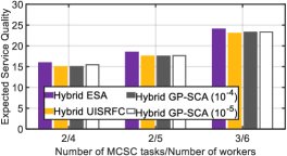
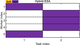
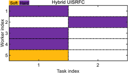
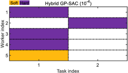
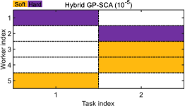
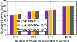
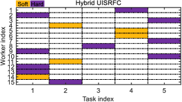
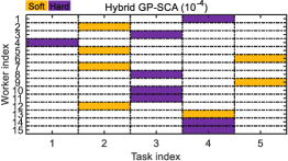
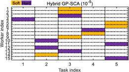
Figure 3: (a). Performance comparison on the expected service quality of MCSC tasks upon considering small problem sizes; (b)$\sim$(e) Long-term contract signing associated with 2 tasks and 5 workers in (a); (f). Performance comparison on the expected service quality of MCSC tasks upon considering large problem sizes; (g)$\sim$(i) Long-term contract signing associated with 5 tasks and 15 workers in (f).

3.2 Temporary Worker Determination (Online Mode)

Owing to the uncertainties (e.g., $\alpha_{i}$ and $\beta_{i}$, $w_{i}\in\mathbb{W}$), the actual service quality offered to a task may not reach its satisfaction during each practical trading. For example, the possible absence of some long-term workers associated with task $\bm{s_{k}}$ during a trading may lead to an unsatisfying overall service quality (e.g., lower than $d_{k}^{Q}$), while the disbursed expense is within budget $d_{k}^{B}$. Under this circumstance, MCSC platform can hire feasible temporary workers, e.g., workers without long-term contracts, under an onsite trading mode. Let $\mathbb{S}^{\prime}$ be the set of tasks with unsatisfying service quality offered from long-term workers with remaining budgets, and $\mathbb{W}^{\prime}$ denote the set of workers without signing long-term contracts with the MCSC platform, who have attended the current trading (namely, for all $w_{i^{\prime}}\in\mathbb{W}^{\prime}$, we have $\alpha_{i^{\prime}}=1$).

The proposed temporary worker determination aims to maximize the overall received quality of tasks in $\mathbb{S}^{\prime}$, under the current network/market condition, as shown by the following optimization problem.

$$\qquad\quad\bm{\mathcal{P}_{6}:}\max\limits_{\mathbb{X}^{\prime}}~{}\sum\limits_{\bm{s_{k^{\prime}}}\in\mathbb{S}^{\prime}}\sum\limits_{w_{i^{\prime}}\in\mathbb{W}^{\prime}}\sum\limits_{\ell\in\bm{L}}x_{i^{\prime},k^{\prime},\ell}q_{i^{\prime},k^{\prime},\ell}$$ (26)

s.t.

$$\text{(C10)}:x_{i^{\prime},k^{\prime},\ell}\in\{0,1\},\forall w_{i^{\prime}}\in\mathbb{W}^{\prime},\bm{s_{k^{\prime}}}\in\mathbb{S}^{\prime},\ell\in\bm{L}$$

$$\text{(C11)}:\sum\limits_{\bm{s_{k^{\prime}}}\in\mathbb{S}^{\prime}}\sum\limits_{\ell\in\bm{L}}x_{i^{\prime},k^{\prime},\ell}\leqslant 1,\forall w_{i^{\prime}}\in\mathbb{W}^{\prime}$$

$$\text{(C12)}:\sum_{w_{i^{\prime}}\in\mathbb{W}^{\prime}}\sum_{\ell\in\bm{L}}x_{i^{\prime},k^{\prime},\ell}p_{i^{\prime},k^{\prime},\ell}\leqslant{\left(d^{B}_{k^{\prime}}\right)}^{\prime},\forall\bm{s_{k^{\prime}}}\in\mathbb{S}^{\prime}$$

In $\bm{\mathcal{P}_{6}}$, $\mathbb{X}^{\prime}=\{x_{i^{\prime},k^{\prime},\ell}|w_{i^{\prime}}\in\mathbb{W}^{\prime},\bm{s_{k^{\prime}}}\in\mathbb{S}^{\prime},\ell\in\bm{L}\}$ denotes the profile of temporary worker determination. Specifically, ${\left(d^{B}_{k^{\prime}}\right)}^{\prime},\forall\bm{s_{k^{\prime}}}\in\mathbb{S}^{\prime}$ represents the remaining budget, while (C12) indicates the corresponding budget constraint.

Since the algorithm design for problem $\bm{\mathcal{P}_{6}}$ is similar to the proposed algorithms in Sec. 3.1.3-3.1.5, we design three online algorithms which are similar to ESA, UISRFC and GP-SCA, where the detailed analysis is thus neglected here to avoid redundancy (the GP format and transferred convex optimization problem associated with $\bm{\mathcal{P}_{6}}$ is detailed in Appendix D).

4 Evaluation

This section presents comprehensive experimental evaluations to demonstrate the validity of our proposed hybrid worker recruitment mechanism for MCSC.

4.1 Settings

Simulations are implemented via MATLAB R2021b platform on desktop computer with $11^{\text{th}}$ Gen Intel Core i7-11700F 2.50GHz CPU and 16.0 GB RAM. Key parameters are set as follows: $a_{i}\in\left[80\%-16\%,80\%+16\%\right]$, $\mu_{w_{i}}\in[3-0.6,3+0.6]$, $\sigma_{w_{i}}\in[0.5-0.1,0.5+0.1]$, $b_{w_{i}}^{-}\in[\mu_{w_{i}}-(1.2-0.24),\mu_{w_{i}}-(1.2+0.24)]$, $b_{w_{i}}^{+}\in[\mu_{w_{i}}+(1.2-0.24),\mu_{w_{i}}+(1.2+0.24)]$, $c_{i,k}\in[1.5-0.3,1.5+0.3]$, $r_{i}\in[0.6,0.8]$, $r_{i}^{\prime}\in[0.1,0.3]$, $q_{i,k,\mathsf{Hard}}\in[4-0.8,4+0.8]$, $d_{i}^{B}\in[15,22]$, $d_{i}^{Q}\in[8-0.8,8+0.8]$, $\lambda^{s_{k}}_{1}\in[1,1.05]$, $\lambda^{s_{k}}_{2}\in[0.95,1]$, $\lambda^{s_{k}}_{3}\in[0.3,0.4]$, $\lambda^{s_{k}}_{4}\in[0.1,0.2]$, $\lambda^{w_{i}}_{1}\in[0.98,1.01]$, $\lambda^{w_{i}}_{2}\in[0.3,0.4]$.

Specifically, our proposed algorithms are abbreviated to “Hybrid ESA”, “Hybrid UISRFC”, and “Hybrid GP-SCA” for analytical simplicity. Besides, three contrast methods associated with online trading mode are considered as baselines, named by “Online ESA”, “Online UISRFC” and “Online GP-SCA”, where all the workers are temporary and each trading is implemented based on the current worker/task/network condition, via applying ESA, UISRFC, and GP-SCA, respectively.

4.2 Performance Analysis

4.2.1 Expected and practical utility of MCSC platform

To demonstrate the advantages of our proposed algorithms associated with hybrid worker recruitment for MCSC in wireless networks, we first analyze the value of expected service quality of MCSC tasks during long-term worker recruitment, as shown by Fig. 3. Figs. 3(a)-3(e) consider small-size networks with 2-3 tasks and 4-6 workers, where $10^{-4}$ and $10^{-5}$ in the legend denote the convergence criterion of GP-SCA. For example, the algorithm will stop at the $m$-th iteration when $|y^{[m]}-y^{[m-1]}|\leqslant 10^{-4}$ by setting $10^{-4}$ as the convergence criterion.

As shown in Fig. 3(a), our proposed Hybrid UISRFC and Hybrid GP-SCA can approach the performance of ESA, with a relatively low computational complexity (which will also be illustrated by Fig. 6). Besides, a tighter convergence criterion (e.g., $10^{-5}$) can help GP-SCA to reach a larger value of expected service quality.

Figs. 3(b)-3(e) describes the long-term contract signing among 2 MCSC tasks and 5 workers, where in Hybrid GP-SCA, the expected service quality of MCSC tasks can be improved roughly by $5.5\%$ when applying $10^{-5}$ as the convergence criterion, rather than $10^{-4}$.

Fig. 3(f) considers large problem sizes, e.g., 5-10 MCSC tasks and 10-16 workers, where Hybrid ESA has been omitted due to its extremely high computational complexity. Similarly, Hybrid GP-SCA ($10^{-5}$) achieves slightly better performance than GP-SCA with convergence criterion $10^{-4}$, while Hybrid GP-SCA outperforms hybrid URIRFC since the performance of the latter depends heavily on the number of iterations and has randomness due to the large solution space and stochastic searching mode.

Figs. 3(g)-3(i) depict how long-term contracts are signed among 5 tasks and 15 workers. Interestingly, our solutions allow a certain overbooking rate to support dynamic service supply since some contractual workers may not be able to offer satisfactory services, due to factors such as their mobility and varying wireless channel qualities. For example, services offered by 4 of the contractual workers $w_{2}$, $w_{9}$, $w_{12}$, $w_{13}$, $w_{14}$ associated with task $s_{1}$ in Fig. 3(g) are sufficient to satisfy $\bm{s_{1}}$’s service quality requirement where the overbooking rate is roughly $(5-4)/4=25\%$.

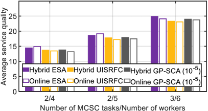
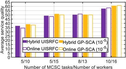
Figure 4: Performance comparison on the average practical service quality (per trading) of MCSC tasks upon considering 1000 trading under different problem sizes.

Figure 4 illustrates the performance on the average practical service quality (per trading) of MCSC tasks from a long-term perspective, with three baseline methods, via considering 1000 trading. Similarly, different problem sizes are considered to prove the advantages and generalization of our proposed hybrid worker recruitment mechanism.

Considering small problem sizes as shown by Fig. 4(a), Hybrid ESA achieves similar average service quality as compared to Online EAS while sometimes can even be better, since our proposed mechanism allows a certain overbooking rate, rather than Online ESA in which each trading is implemented under strict budget constraints. Besides, UISRFC and GP-SCA obtain slightly lower performance, while the proposed Hybrid UISRFC and Hybrid GP-SCA outperform Online UISRFC and Online GP-SCA thanks to overbooking. Although in some trading our proposed algorithms may exceed the corresponding budget (caused by probabilistic constraints), the expense from long-term perspective is often acceptable (which will be discussed in Fig. 6).

Fig. 4(b) considers large size problems via setting $10^{-5}$ as the convergence criterion of GP-SCA. As can be seen, our proposed Hybrid UISRFC and Hybrid GP-SCA can reach similar average service quality performance to that of the corresponding online trading methods, while sometimes obtaining slightly better performance in scenarios with rather large number of workers (e.g., 5 tasks and 15 workers in Fig. 4(b)), since the proposed overbooking can help with recruiting more long-term workers, under acceptable over-budget risks. For example, revisiting Fig. 3(i), task $s_{5}$ can obtain commendable service quality during a trading when all the contractual workers $w_{2}$, $w_{9}$, $w_{11}$, $w_{15}$ have participated in trading, which cause an over-budget issue. Moreover, our proposed hybrid worker recruitment offers commendable time efficiency as compared to online trading methods, as shown by Fig. 6.

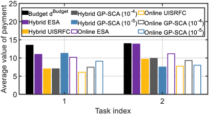
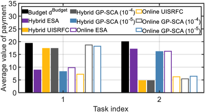
Figure 5: Performance comparison on $d_{k}^{B}$ and the average practical expense of MCSC tasks for purchasing workers’ services (per trading), upon considering 2 tasks, 5 workers, and different values of budget, under 1000 trading: (a). $d^{B}_{k}\in[13,15]$; (b). $d^{B}_{k}\in[18,20]$.

4.2.2 Budget and payment

Figure 5 compares the average practical expense of each MCSC task (per trading) for purchasing sensing and computing services from workers, as well as the corresponding budget, from a long-term perspective over simulating 1000 trading. As can be seen in Figs. 5(a) and Fig. 5(b), although overbooking is encouraged in our proposed hybrid worker recruitment mechanism, the average payment of each MCSC task to recruited workers is still acceptable, as benefited from the well-designed risk controlling constraint (e.g., constraint (C2) of problem $\bm{\mathcal{P}_{1}}$). For example, considering $\lambda_{2}^{s_{1}}=0.98$ and $\lambda_{4}^{s_{1}}=0.1$, the risk (namely, probability) of task $\bm{s_{1}}$’s payment to sensing and computing services exceeds $98\%\times d^{B}_{1}$ will be controlled within $10\%$. In addition, our proposed mechanism can achieve better service quality for tasks while greatly reducing the decision-making time (running time, as illustrated by Fig. 6) under a larger budget.

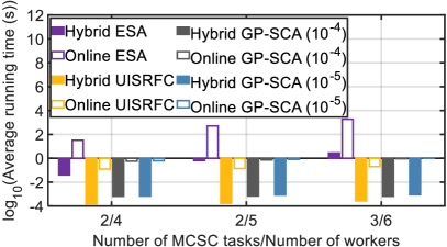
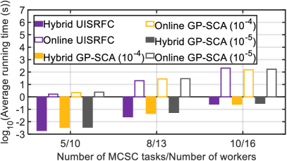
Figure 6: Running time performance under different problem sizes.

4.2.3 Running time

Figure 6 analyzes performance measured as the average running time (per trading), for 1000 trading, upon considering small and large problem sizes. Logarithmic function is utilized (in the y-axis) to better illustrate the gap between different algorithms. As can be observed from Fig. 6(a), ESA-based algorithms always incur a large running time to reach the final worker recruitment solution, where our proposed Hybrid ESA, Hybrid UISRFC and Hybrid GP-SCA greatly outperform the corresponding online methods, thanks to the pre-signed long-term contracts. Conventional online trading mode should make a decision based on the current network/worker/task information during every trading, which thus incurs a certain delay on decision-making, especially for ESA-based algorithm. For example, the running time associated with Online ESA reaches over 500 seconds averagely (see Fig. 6(a)), during each trading when considering 2 tasks and 5 workers, which makes it impractical to be implemented in real-world networks particularly with energy-constrained mobile devices. Although Online UISRFC and Online GP-SCA obtain far better running time performance than Online ESA, the accumulated delay with the increasing number of trading will bring challenges to the long-term development of MCSC networks. For example, Online GP-SCA ($10^{-5}$) (Fig. 6(a), 2 tasks and 4 workers) causes around 0.6196 seconds decision-making delay on average, that may be practicable during one trading, which, however, will cost around 619.6 seconds over 100 trading. For large problem sizes shown by Fig. 6(b), our proposed Hybrid UISRFC and Hybrid GP-SCA can still offer commendable running time, as benefited by pre-determined long-term workers. On the contrary, running time associated with Online UISRFC and Online GP-SCA gradually become prohibitive with increasing number of workers and tasks.

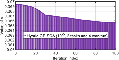
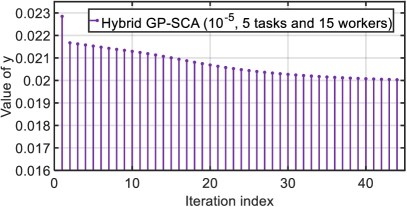
Figure 7: Convergence performance on solving GP problem $\bm{\mathcal{P}_{5}}$ by the proposed GP-SCA.

4.2.4 Convergence of GP-SCA

Figure 7 illustrates how our GP-SCA-based solution for $\bm{\mathcal{P}_{5}}$ converges to its given convergence criterion ($10^{-5}$). As can be seen from Fig. 7(a) and Fig. 7(b), the proposed GP-SCA can always exhibit a good performance on convergence, upon considering different problem sizes.

In conclusion, the proposed hybrid worker recruitment mechanism for mobile crowd sensing and computing that integrates both online and offline trading modes achieves good performance on service quality in comparison with online trading modes, while offering far better time efficiency, which provides a commendable reference for the long-term and continuable development of future MCSC networks.

5 Conclusion

This paper proposes a novel risk-aware hybrid worker recruitment mechanism for MCSC under uncertainties, via unifying both online (long-term worker recruitment) and offline (temporary worker recruitment) trading modes. The problems are formulated as 0-1 integer linear programming, which is NP-hard. Thus, three algorithms, namely, exhaustive searching, unique index-based stochastic searching with risk-aware filter constraint, and geometric programming-based successive convex algorithm, are designed to achieve the optimal (with high computational complexity) or sub-optimal (with low computation complexity) solutions. Comprehensive simulations demonstrate the effectiveness of our proposed mechanism, in comparison to conventional trading methods. Several future directions such as the cooperation among workers, as well as cost-effective and time-efficient algorithm design for the formulated NP-hard problems can be pursued.

Appendix A Analysis of $\mathbb{P}^{*}$

For a worker $w_{i}\in\mathbb{W}$, the tolerable payment $p_{i,k,\mathsf{Hard}}$ and $p_{i,k,\mathsf{Soft}}$ under hard/soft assurance can be determined by constraints (C3) and (C6).

$\bullet$Derivation on $p_{i,k,\mathsf{Soft}}^{*}$ (payment associated with soft assurance): We first analyze the acceptable payment $p_{i,k,\mathsf{Soft}}^{*}$ when a worker $w_{i}$ offers service to sensing task $\bm{s_{k}}$ under soft quality assurance. Assume that $x_{i,k,\mathsf{Soft}}=1$, risk of worker $w_{i}$ is calculated by the following (27).

$$\mathcal{R}^{w_{i}}(x_{i,k,\mathsf{Soft}}=1,q_{i,k,\mathsf{Soft}},p_{i,k,\mathsf{Soft}},\beta_{i})$$

$$=\operatorname{Pr}\left\{p_{i,k,\mathsf{Soft}}\leqslant\lambda_{1}^{w_{i}}\mathcal{U}^{min}+c_{i,k}\right\}$$ (27)

Apparently, $p_{i,k,\mathsf{Soft}}^{*}$ should satisfy the following inequality (28) to meet constraint (C3),

$$p_{i,k,\mathsf{Soft}}^{*}>\lambda_{1}^{w_{i}}\mathcal{U}^{min}+c_{i,k}$$ (28)

In this case, we have the expected utility of worker $w_{i}$ as given in (29).

$$\overline{\mathcal{U}^{w_{i}}}(x_{i,k,\mathsf{Soft}}=1,q_{i,k,\mathsf{Soft}},p_{i,k,\mathsf{Soft}},\alpha_{i},\beta_{i})$$

$$=a_{i}\left(p_{i,k,\mathsf{Soft}}-c_{i,k}\right)$$ (29)

Thus, the acceptable payment $p_{i,k,\mathsf{Soft}}^{*}$ can be defined by (30), to meeting constraints (C3) and (C6), where $\Delta p$ denotes a standard incentive agreed by all the participants in the MCSC network.

$$p_{i,k,\mathsf{Soft}}^{*}=\text{max}\left(\lambda_{1}^{w_{i}}\mathcal{U}^{min}+c_{i,k},c_{i,k}\right)+\Delta p$$

$$=\lambda_{1}^{w_{i}}\mathcal{U}^{min}+c_{i,k}+\Delta p$$ (30)

$\bullet$Derivation on $p_{i,k,\mathsf{Hard}}^{*}$ (payment associated with hard assurance): Assume that $x_{i,k,\mathsf{Hard}}=1$, we have the following (31):

$$\mathcal{R}^{w_{i}}\left(x_{i,k,\mathsf{Hard}}=1,q_{i,k,\mathsf{Hard}},p_{i,k,\mathsf{Hard}},\alpha_{i},\beta_{i}\right)$$

$$=\operatorname{Pr}\left\{-\xi_{i}r_{i}q_{i,k,\mathsf{Hard}}\beta_{i}+p_{i,k,\mathsf{Hard}}-c_{i,k}\leqslant\lambda_{i}^{w_{i}}\mathcal{U}^{min}\right\}$$

$$=1-\operatorname{Pr}\left\{\xi_{i}r_{i}q_{i,k,\mathsf{Hard}}\beta_{i}\leqslant p_{i,k,\mathsf{Hard}}c_{i,k}-\lambda_{i}^{w_{i}}\mathcal{U}^{min}\right\}$$ (31)

Let random variable $Y=\xi_{i}q_{i,k,\mathsf{Hard}}r_{i}\beta_{i}$ for notational simplicity. According to the distribution of $\beta_{i}$, we have $Y$ conditional on $\mathbbm{y}^{-}\leqslant Y\leqslant\mathbbm{y}^{+}$ associated with Normal Distribution with mean $\mu_{Y}=\xi_{i}r_{i}q_{i,k,\mathsf{Hard}}\mu_{w_{i}}$ and variance ${(\sigma_{Y})}^{2}={(\xi_{i}r_{i}q_{i,k,\mathsf{Hard}}\sigma_{w_{i}})}^{2}$, which thus follows a Truncated Normal Distribution denoted by $Y\sim\text{N}\left(\mu_{Y},{(\sigma_{Y})}^{2},\mathbbm{y}^{-},\mathbbm{y}^{+}\right)$. Specifically, $\mathbbm{y}^{-}=\xi_{i}r_{i}q_{i,k,\mathsf{Hard}}b_{w_{i}}^{-}$, and $\mathbbm{y}^{+}=\xi_{i}r_{i}q_{i,k,\mathsf{Hard}}b_{w_{i}}^{+}$ indicates the lower and upper bound of Y, respectively. Thus, CDF of $Y$ is given in (32).

$$\text{F}_{Y}(Y\leqslant y)=\begin{cases}0,~{}~{}~{}y<\mathbbm{y}^{-}\\ \frac{\Phi\left(\frac{y-\mu_{Y}}{\sigma_{Y}}\right)-\Phi\left(\frac{\mathbbm{y}^{-}-\mu_{Y}}{\sigma_{Y}}\right)}{\Phi\left(\frac{\mathbbm{y}^{+}-\mu_{Y}}{\sigma_{Y}}\right)-\Phi\left(\frac{\mathbbm{y}^{-}-\mu_{Y}}{\sigma_{Y}}\right)}\\ 1,~{}~{}~{}y>\mathbbm{y}^{+}\end{cases}$$ (32)

According to (32), (31) can be rewritten by (33),

$$\mathcal{R}^{w_{i}}\left(x_{i,k,\mathsf{Hard}}=1,q_{i,k,\mathsf{Hard}},p_{i,k,\mathsf{Hard}},\alpha_{i},\beta_{i}\right)$$

$$=1-\text{F}_{Y}\left(Y\leqslant p_{i,k,\mathsf{Hard}}-c_{i,k}-\lambda_{1}^{w_{i}}\mathcal{U}^{min}\right)$$

$$\begin{cases}0,p_{i,k,\mathsf{Hard}}-c_{i,k}-\lambda_{1}^{w_{i}}\mathcal{U}^{min}>\mathbbm{y}^{+}\\ 1-\frac{\Phi\left(\frac{p_{i,k,\mathsf{Hard}}-c_{i,k}-\lambda_{1}^{w_{i}}\mathcal{U}^{min}-\mu_{Y}}{\sigma_{Y}}\right)-\Phi\left(\frac{\mathbbm{y}^{-}-\mu_{Y}}{\sigma_{Y}}\right)}{\Phi\left(\frac{\mathbbm{y}^{+}-\mu_{Y}}{\sigma_{Y}}\right)-\Phi\left(\frac{\mathbbm{y}^{-}-\mu_{Y}}{\sigma_{Y}}\right)},\\ \mathbbm{y}^{-}\leqslant p_{i,k,\mathsf{Hard}}-c_{i,k}-\lambda_{1}^{w_{i}}\mathcal{U}^{min}\leqslant\mathbbm{y}^{+}\\ 1,p_{i,k,\mathsf{Hard}}-c_{i,k}-\lambda_{1}^{w_{i}}\mathcal{U}^{min}<\mathbbm{y}^{-}\end{cases}$$ (33)

In constraint (C3), $\lambda_{2}^{w_{i}}\in[0,1)$ where $\lambda_{2}^{w_{i}}=0$ means worker $w_{i}$ does not accept any risk. Consequently, $p_{i,k,\mathsf{Hard}}^{*}$ should meet the following inequalities:

$$\left\{\begin{array}[]{l}p_{i,k,\mathsf{Hard}}-c_{i,k}-\lambda_{1}^{w_{i}}\mathcal{U}^{min}>\mathbbm{y}^{-}\qquad\qquad\qquad\quad\quad~{}~{}\text{(34a)}\\ 1-\frac{\Phi\left(\frac{p_{i,k,\mathsf{Hard}}-c_{i,k}-\lambda_{1}^{w_{i}}\mathcal{U}^{min}-\mu_{Y}}{\sigma_{Y}}\right)-\Phi\left(\frac{\mathbbm{y}^{-}-\mu_{Y}}{\sigma_{Y}}\right)}{\Phi\left(\frac{\mathbbm{y}^{+}-\mu_{Y}}{\sigma_{Y}}\right)-\Phi\left(\frac{\mathbbm{y}^{-}-\mu_{Y}}{\sigma_{Y}}\right)}\leqslant\lambda_{2}^{w_{i}}\text{(34b)}\end{array}\right.$$

From (34a), we have (35),

$$p_{i,k,\mathsf{Hard}}^{*}>\lambda_{1}^{w_{i}}\mathcal{U}^{min}+c_{i,k}+\xi_{i}r_{i}q_{i,k,\mathsf{Hard}}b_{w_{i}}^{-}$$ (35)

As for (34b), we have the following (36). Since error function erf(.) represents a non-elementary function which pose challenges to have a close form of $p_{i,k,\mathsf{Hard}}^{*}$. Thus, let $\widehat{p_{i,k,\mathsf{Hard}}^{*}}$ be the minimum tolerable value of payment $p_{i,k,\mathsf{Hard}}$ that meets inequation $\text{erf}\left(\frac{p_{i,k,\mathsf{Hard}}-c_{i,k}-\lambda_{1}^{w_{i}}\mathcal{U}^{min}-\mu_{Y})}{\sqrt{2}\sigma_{Y}}\right)\geqslant 2\mathbbm{c}_{i}-1$ given by (36), for notational simplicity. Then, considering constraint C5 under $x_{i,k,\mathsf{Hard}}=1$, we have (37). In conclusion, for all $w_{i}\in\mathbb{W}$, $\bm{s_{k}}\in\mathbb{S}$, $p_{i,k,\mathsf{Hard}}^{*}$ can be defined by (38).

$$1-\frac{\Phi\left(\frac{p_{i,k,\mathsf{Hard}}-c_{i,k}-\lambda_{1}^{w_{i}}\mathcal{U}^{min}-\mu_{Y}}{\sigma_{Y}}\right)-\Phi\left(\frac{\mathbbm{y}^{-}-\mu_{Y}}{\sigma_{Y}}\right)}{\Phi\left(\frac{\mathbbm{y}^{+}-\mu_{Y}}{\sigma_{Y}}\right)-\Phi\left(\frac{\mathbbm{y}^{-}-\mu_{Y}}{\sigma_{Y}}\right)}\leqslant\lambda_{2}^{w_{i}}\xLongrightarrow$$

$$\Phi\left(\frac{p_{i,k,\mathsf{Hard}}-c_{i,k}-\lambda_{1}^{w_{i}}\mathcal{U}^{min}-\mu_{Y}}{\sigma_{Y}}\right)\geqslant\mathbbm{c}_{i}\Rightarrow\int_{-\infty}^{\frac{p_{i,k,\mathsf{Hard}}-c_{i,k}-\lambda_{1}^{w_{i}}\mathcal{U}^{min}-\mu_{Y}}{\sigma_{Y}}}\exp\left(-\frac{t^{2}}{2}\right)dt\geqslant\sqrt{2\pi}\mathbbm{c}_{i}$$

$${\Rightarrow}\sqrt{\frac{\pi}{2}}\operatorname{erf}\left(\frac{p_{i,k,\mathsf{Hard}}-c_{i,k}-\lambda_{1}^{w_{i}}\mathcal{U}^{min}-\mu_{Y}}{\sqrt{2}\sigma_{Y}}\right)+\sqrt{\frac{\pi}{2}}\geqslant\sqrt{2\pi}\mathbbm{c}_{i}\Rightarrow\operatorname{erf}\left(\frac{p_{i,k,\mathsf{Hard}}-c_{i,k}-\lambda_{1}^{w_{i}}\mathcal{U}^{min}-\mu_{Y}}{\sqrt{2}\sigma_{Y}}\right)\geqslant 2\mathbbm{c}_{i}-1$$ (36)

$$\overline{\mathcal{U}^{w_{i}}}\left(x_{i,k,\mathsf{Hard}}=1,q_{i,k,\mathsf{Hard}},p_{i,k,\mathsf{Hard}},\alpha_{i},\beta_{i}\right)=a_{i}(p_{i,k,\mathsf{Hard}}-c_{i,k,})-\xi_{i}r_{i}a_{i}q_{i,k,\mathsf{Hard}}\overline{\beta_{i}}$$

$${\Longrightarrow}~{}p_{i,k,\mathsf{Hard}}>\xi_{i}r_{i}q_{i,k,\mathsf{Hard}}\overline{\beta_{i}}+c_{i,k}$$ (37)

$$p_{i,k,\mathsf{Hard}}^{*}=\text{max}\left(\lambda_{1}^{w_{i}}\mathcal{U}^{min}+c_{i,k}+\xi_{i}r_{i}q_{i,k,\mathsf{Hard}}b_{w_{i}}^{-};~{}\widehat{p_{i,k,\mathsf{Hard}}^{*}};~{}\xi_{i}r_{i}q_{i,k,\mathsf{Hard}}\overline{\beta_{i}}+c_{i,k}\right)+\Delta p$$ (38)

Appendix B Analysis of Constraints (C1) and (C7)

Notably, it is difficult to obtain exact tractable forms for $\mathcal{R}_{1}^{s_{k}}\left(\mathbb{X},\mathbb{Q},\mathbb{A}\right)$ and $\mathcal{R}_{2}^{s_{k}}\left(\mathbb{X},\mathbb{P}^{*},\mathbb{A}\right)$ since they contain mixed random variables that are independent with different distributions. Let $\mathbb{I}_{k,\mathsf{Hard}}$ and $\mathbb{I}_{k,\mathsf{Soft}}$ denote the set of workers which are hired to offer hard assurance, and soft assurance of sensing service for task $\bm{s_{k}}$, respectively, for notational simplicity ($\mathbb{I}_{k,\mathsf{Hard}}\cap\mathbb{I}_{k,\mathsf{Soft}}=\emptyset$). For example, obtaining the value range of $\sum_{w_{i}\in\mathbb{W}}\sum_{\ell\in\bm{L}}\alpha_{i}x_{i,k,\ell}q_{i,k,\ell}$ in $\mathcal{R}_{1}^{s_{k}}(\mathbb{X},\mathbb{Q},\mathbb{A})$ needs considering $2+C_{|\mathbb{I}_{k,\ell^{\prime}}|}^{1}+C_{|\mathbb{I}_{k,\ell^{\prime}}|}^{2}+\cdots+C_{|\mathbb{I}_{k,\ell^{\prime}}|}^{|\mathbb{I}_{k,\ell^{\prime}}|-1}$ possible situations (where $\ell^{\prime}=$ “Soft”); while (C7) needs considering $2+C_{\sum_{\ell\in\bm{L}}|\mathbb{I}_{k,\ell}|}^{1}+C_{\sum_{\ell\in\bm{L}}|\mathbb{I}_{k,\ell}|}^{2}+\cdots+C_{\sum_{\ell\in\bm{L}}|\mathbb{I}_{k,\ell}|}^{\sum_{\ell\in\bm{L}}|\mathbb{I}_{k,\ell}|-1}$ possible situations, which further pose challenges on analyzing risk-related constraints.

We first rewrite constraint (C1) as inequality (39). Then, to obtain a tractable expression of the $\operatorname{Pr}\{\}$ in (39), we obtain (40) according to Markov inequality [20], where (C1) is turned into (41) based on (39) and (40). Similarly, to obtain a tractable expression, $\mathcal{R}_{2}^{s_{k}}(\mathbb{X},\mathbb{P}^{*},\mathbb{A})$ is rewritten as the following (42), which uses the result of Markov inequality. Constraints (C7) can thus be obtained as (43).

$$\mathcal{R}_{1}^{s_{k}}\left(\mathbb{X},\mathbb{Q},\mathbb{A}\right)\leqslant\lambda_{3}^{s_{k}}\Longrightarrow\operatorname{Pr}\left\{{\sum_{w_{i}\in\mathbb{W}}\sum\limits_{\ell\in\bm{L}}\alpha_{i}x_{i,k,\ell}q_{i,k,\ell}}>\lambda_{1}^{s_{k}}d_{k}^{Q}\right\}\geqslant 1-\lambda_{3}^{s_{k}}$$ (39)

$$\operatorname{Pr}\left\{{\sum_{w_{i}\in\mathbb{W}}\sum\limits_{\ell\in\bm{L}}\alpha_{i}x_{i,k,\ell}q_{i,k,\ell}}>\lambda_{1}^{s_{k}}d_{k}^{Q}\right\}\leqslant\operatorname{Pr}\left\{{\sum_{w_{i}\in\mathbb{W}}\sum\limits_{\ell\in\bm{L}}\alpha_{i}x_{i,k,\ell}q_{i,k,\ell}}\geqslant\lambda_{1}^{s_{k}}d_{k}^{Q}\right\}$$

$$\leqslant\frac{\text{E}\left[\sum\limits_{w_{i}\in\mathbb{W}}\sum\limits_{\ell\in\bm{L}}\alpha_{i}x_{i,k,\ell}q_{i,k,\ell}\right]}{\lambda_{1}^{s_{k}}d_{k}^{Q}}=\frac{\sum\limits_{w_{i}\in\mathbb{W}}\sum\limits_{\ell\in\bm{L}}a_{i}x_{i,k,\ell}\overline{q_{i,k,\ell}}}{\lambda_{1}^{s_{k}}d_{k}^{Q}}$$ (40)

$$\text{(C1)}^{\prime}:~{}\frac{\sum\limits_{w_{i}\in\mathbb{W}}\sum\limits_{\ell\in\bm{L}}a_{i}x_{i,k,\ell}\overline{q_{i,k,\ell}}}{\lambda_{1}^{s_{k}}d_{k}^{Q}}\geqslant 1-\lambda_{3}^{s_{k}},\forall\bm{s_{k}}\in\mathbb{S}$$ (41)

$$\mathcal{R}_{2}^{s_{k}}\left(\mathbb{X},\mathbb{P}^{*},\mathbb{A}\right)=\operatorname{Pr}\left\{\sum\limits_{w_{i}\in\mathbb{W}}\sum\limits_{\ell\in\bm{L}}\alpha_{i}x_{i,k,\ell}p_{i,k,\ell}^{*}>\lambda_{2}^{s_{k}}d_{k}^{B}\right\}\leqslant\operatorname{Pr}\left\{\sum_{w_{i}\in\mathbb{W}}\sum\limits_{\ell\in\bm{L}}\alpha_{i}x_{i,k,\ell}p_{i,k,\ell}^{*}\geqslant\lambda_{2}^{s_{k}}d_{k}^{B}\right\}$$

$$\leqslant\frac{\text{E}\left[\sum\limits_{w_{i}\in\mathbb{W}}\sum\limits_{\ell\in\bm{L}}\alpha_{i}x_{i,k,\ell}p_{i,k,\ell}^{*}\right]}{\lambda_{2}^{s_{k}}d_{k}^{B}}=\frac{\sum\limits_{w_{i}\in\mathbb{W}}\sum\limits_{\ell\in\bm{L}}a_{i}x_{i,k,\ell}p_{i,k,\ell}^{*}}{\lambda_{2}^{s_{k}}d_{k}^{B}}$$ (42)

$$\text{(C7)}^{\prime}:~{}\frac{\sum\limits_{w_{i}\in\mathbb{W}}\sum\limits_{\ell\in\bm{L}}a_{i}x_{i,k,\ell}p_{i,k,\ell}^{*}}{\lambda_{2}^{s_{k}}d_{k}^{B}}\leqslant\lambda_{4}^{s_{k}},\forall\bm{s_{k}}\in\mathbb{S}$$ (43)

Appendix C Analysis of (25)

First, let variable $u_{i,k,\ell}\triangleq\ln{x_{i,k,\ell}}$, and $v\triangleq\ln y$; while $\mathbbm{u}={\{u_{i,k,\ell}\}}_{w_{i}\in\mathbb{W},\bm{s_{k}}\in\mathbb{S},\ell\in\bm{L}}$ for notational simplicity. By applying $z_{i,k,\ell}$ and $v$, $\bm{\mathcal{P}_{5}}$ is reformulated by a standard convex optimization problem, as the following (44).

$$\min\limits_{\mathbb{X},y}y\Rightarrow\min\limits_{\mathbbm{u},v}\text{e}^{v}$$ (44)

Constraints ${(\hat{\text{C}}\text{1})}^{\prime},\text{(C5)},{\text{(C7)}}^{\prime},{(\hat{\text{C}}\text{8})}^{\prime},(\hat{\text{C}}\text{9})$ can be transferred by the following (45)-(50), by applying the logarithmic change of variables. Specifically, similar to ${\bm{x}}^{[m]}$, let ${\mathbbm{u}}^{[m]}=\left\{u_{i,k,\ell}^{[m]}\right\}$, and $v^{[m]}$ denote the solution of $m$-th iteration. Based on the above discussions, problem $\bm{\mathcal{P}_{5}}$ is reformulated as $\bm{\mathcal{P}_{7}}$ given in (51), which is a typical convex optimization problem.

$${(\hat{\text{C}}\text{1})}^{\prime}:\forall\bm{s_{k}}\in\mathbb{S}$$

$$\frac{(1-\lambda_{3}^{s_{k}})\lambda_{1}^{s_{k}}d_{k}^{Q}}{\prod\limits_{w_{i}\in\mathbb{W}}\prod\limits_{\ell\in\bm{L}}{\left(\frac{\text{e}^{u_{i,k,\ell}}f_{k}^{(C1)}{\left(\text{e}^{\mathbbm{u}^{[m-1]}}\right)}}{\text{e}^{u_{i,k,\ell}^{[m-1]}}}\right)}^{\frac{a_{i}\overline{q_{i,k,\ell}}\text{e}^{u_{i,k,\ell}^{[m-1]}}}{f_{k}^{(C1)}\left(\text{e}^{\mathbbm{u}^{[m-1]}}\right)}}}\leqslant 1,$$ (45)

$$\text{(C4)}^{\prime}:u_{i,k,\ell}\leqslant 0,\forall w_{i}\in\mathbb{W},\bm{s_{k}}\in\mathbb{S},\ell\in\bm{L}$$ (46)

$$\text{(C5)}:\sum_{\bm{s_{k}}\in\mathbb{S}}\sum_{\ell\in\bm{L}}\text{e}^{u_{i,k,\ell}}\leqslant 1,\forall w_{i}\in\mathbb{W}$$ (47)

$${\text{(C7)}}^{\prime}:\frac{{\sum\limits_{w_{i}\in\mathbb{W}}\sum\limits_{\ell\in\bm{L}}a_{i}p_{i,k,\ell}^{*}\text{e}^{u_{i,k,\ell}}}}{\lambda_{2}^{s_{k}}\lambda_{4}^{s_{k}}d_{k}^{B}}\leqslant 1,\forall\bm{s_{k}}\in\mathbb{S}$$ (48)

$${(\hat{\text{C}}\text{8})}^{\prime}:\frac{\sum\limits_{w_{i}\in\mathbb{W}}\sum\limits_{\bm{s_{k}}\in\mathbb{S}}\sum\limits_{\ell\in\bm{L}}\text{e}^{u_{i,k,\ell}}}{\prod\limits_{w_{i}\in\mathbb{W}}\prod\limits_{\bm{s_{k}}\in\mathbb{S}}\prod\limits_{\ell\in\bm{L}}{\left(\frac{\left(\mu^{\prime}+\text{e}^{2u_{i,k,\ell}}\right)f^{(C8)}\left(\text{e}^{\mathbbm{u}^{[m-1]}}\right)}{\mu^{\prime}+\text{e}^{2u_{i,k,\ell}^{[m-1]}}}\right)}^{\frac{{\mu^{\prime}+\text{e}^{2u_{i,k,\ell}^{[m-1]}}}}{f^{(C8)}\left(\text{e}^{\mathbbm{u}^{[m-1]}}\right)}}}\leqslant 1$$ (49)

$$(\hat{\text{C}}\text{9}):\frac{1}{\prod\limits_{w_{i}\in\mathbb{W}}\prod\limits_{\bm{s_{k}}\in\mathbb{S}}\prod\limits_{\ell\in\bm{L}}{\left(\frac{\text{e}^{(v+u_{i,k,\ell})}f^{(C9)}\left(\text{e}^{\mathbbm{u}^{[m-1]}},\text{e}^{v^{[m-1]}}\right)}{\text{e}^{\left(v^{[m-1]}+u_{i,k,\ell}^{[m-1]}\right)}}\right)}^{\frac{a_{i}\overline{q_{i,k,\ell}}\text{e}^{\left(v^{[m-1]}+u_{i,k,\ell}^{[m-1]}\right)}}{f^{(C9)}\left(\text{e}^{\mathbbm{u}^{[m-1]}},\text{e}^{v^{[m-1]}}\right)}}}\leqslant 1$$ (50)

$$\qquad\qquad\qquad\qquad\qquad\qquad\qquad\qquad\qquad\qquad\qquad\bm{\mathcal{P}_{7}:}\min\limits_{\mathbbm{u},v}\text{e}^{v}$$ (51)

$$\textrm{s.t.}~{}\text{(C4)}^{\prime},$$

$${(\hat{\text{C}}\text{1})}^{\prime}:\ln\left({(1-\lambda_{3}^{s_{k}})\lambda_{1}^{s_{k}}d_{k}^{Q}}\right)-\sum\limits_{w_{i}\in\mathbb{W}}\sum\limits_{\ell\in\bm{L}}\ln\left({\left(\frac{f_{k}^{(C1)}\left(\text{e}^{\mathbbm{u}^{[m-1]}}\right)}{\text{e}^{u_{i,k,\ell}^{[m-1]}}}\right)}^{\frac{a_{i}\overline{q_{i,k,\ell}}\text{e}^{u_{i,k,\ell}^{[m-1]}}}{f_{k}^{(C1)}\left(\text{e}^{\mathbbm{u}^{[m-1]}}\right)}}\right)$$

$$-\sum\limits_{w_{i}\in\mathbb{W}}\sum\limits_{\ell\in\bm{L}}{\frac{a_{i}\overline{q_{i,k,\ell}}\text{e}^{u_{i,k,\ell}^{[m-1]}}u_{i,k,\ell}}{f_{k}^{(C1)}\left(\text{e}^{\mathbbm{u}^{[m-1]}}\right)}}\leqslant 0,\forall\bm{s_{k}}\in\mathbb{S}$$

$$\text{(C5)}:\ln\left(\sum\limits_{\bm{s_{k}}\in\mathbb{S}}\sum\limits_{\ell\in\bm{L}}\text{e}^{u_{i,k,\ell}}\right)\leqslant 0,\forall w_{i}\in\mathbb{W}$$

$${\text{(C7)}}^{\prime}:\ln\left(\frac{{\sum\limits_{w_{i}\in\mathbb{W}}\sum\limits_{\ell\in\bm{L}}a_{i}p_{i,k,\ell}^{*}\text{e}^{u_{i,k,\ell}}}}{\lambda_{2}^{s_{k}}\lambda_{4}^{s_{k}}d_{k}^{B}}\right)\leqslant 0\Rightarrow\ln\left(\sum\limits_{w_{i}\in\mathbb{W}}\sum\limits_{\ell\in\bm{L}}a_{i}p_{i,k,\ell}^{*}\text{e}^{u_{i,k,\ell}}\right)-\ln\left(\lambda_{2}^{s_{k}}\lambda_{4}^{s_{k}}d_{k}^{B}\right)\leqslant 0,\forall\bm{s_{k}}\in\mathbb{S}$$

$${(\hat{\text{C}}\text{8})}^{\prime}:\ln\left(\sum\limits_{w_{i}\in\mathbb{W}}\sum\limits_{\bm{s_{k}}\in\mathbb{S}}\sum\limits_{\ell\in\bm{L}}\text{e}^{u_{i,k,\ell}}\right)-\sum\limits_{w_{i}\in\mathbb{W}}\sum\limits_{\bm{s_{k}}\in\mathbb{S}}\sum\limits_{\ell\in\bm{L}}\ln\left({\left(\frac{f^{(C8)}\left(\text{e}^{\mathbbm{u}^{[m-1]}}\right)}{\mu^{\prime}+\text{e}^{2u_{i,k,\ell}^{[m-1]}}}\right)}^{\frac{{\mu^{\prime}+\text{e}^{2u_{i,k,\ell}^{[m-1]}}}}{f^{(C8)}\left(\text{e}^{\mathbbm{u}^{[m-1]}}\right)}}\right)-$$

$$\sum\limits_{w_{i}\in\mathbb{W}}\sum\limits_{\bm{s_{k}}\in\mathbb{S}}\sum\limits_{\ell\in\bm{L}}\ln\left({\left(\mu^{\prime}+\text{e}^{2u_{i,k,\ell}}\right)}^{\frac{{\mu^{\prime}+\text{e}^{2u_{i,k,\ell}^{[m-1]}}}}{f^{(C8)}\left(\text{e}^{\mathbbm{u}^{[m-1]}}\right)}}\right)\leqslant 0$$

$$(\hat{\text{C}}\text{9}):-\sum\limits_{w_{i}\in\mathbb{W}}\sum\limits_{\bm{s_{k}}\in\mathbb{S}}\sum\limits_{\ell\in\bm{L}}\ln\left({\left(\frac{f^{(C9)}\left(\text{e}^{\mathbbm{u}^{[m-1]}},\text{e}^{v^{[m-1]}}\right)}{\text{e}^{\left(v^{[m-1]}+u_{i,k,\ell}^{[m-1]}\right)}}\right)}^{{\frac{a_{i}\overline{q_{i,k,\ell}}\text{e}^{\left(v^{[m-1]}+u_{i,k,\ell}^{[m-1]}\right)}}{f^{(C9)}\left(\text{e}^{\mathbbm{u}^{[m-1]}},\text{e}^{v^{[m-1]}}\right)}}}\right)$$

$$-\sum\limits_{w_{i}\in\mathbb{W}}\sum\limits_{\bm{s_{k}}\in\mathbb{S}}\sum\limits_{\ell\in\bm{L}}\frac{\left(v+u_{i,k,\ell}\right)a_{i}\overline{q_{i,k,\ell}}\text{e}^{\left(v^{[m-1]}+u_{i,k,\ell}^{[m-1]}\right)}}{f^{(C9)}\left(\text{e}^{\mathbbm{u}^{[m-1]}},\text{e}^{v^{[m-1]}}\right)}\leqslant 0$$

Appendix D Analysis of (26)

The Standard GP format of temporary worker recruitment $\bm{\mathcal{P}_{6}}$ is shown by the following $\bm{\mathcal{P}_{8}}$.

$$\bm{\mathcal{P}_{8}:}\min\limits_{\mathbb{X}^{\prime},y^{\prime}}~{}y^{\prime}$$ (52)

$$\textrm{s.t.}~{}\text{(C11)},$$

$$\text{(C12)}:\frac{\sum\limits_{w_{i^{\prime}}\in\mathbb{W}^{\prime}}\sum\limits_{\ell\in\bm{L}}x_{i^{\prime},k^{\prime},\ell}p_{i^{\prime},k^{\prime},\ell}}{\left(d^{B}_{k^{\prime}}\right)^{\prime}}\leqslant 1,\forall\bm{s_{k^{\prime}}}\in\mathbb{S}^{\prime}$$

$$\text{(C13)}:0\leqslant x_{i^{\prime},k^{\prime},\ell}\leqslant 1,\forall w_{i^{\prime}}\in\mathbb{W}^{\prime},\bm{s_{k^{\prime}}}\in\mathbb{S}^{\prime},\ell\in\bm{L}$$

$$\text{(C14)}:\frac{\sum\limits_{w_{i^{\prime}}\in\mathbb{W}^{\prime}}\sum\limits_{\bm{s_{k^{\prime}}}\in\mathbb{S}^{\prime}}\sum\limits_{\ell\in\bm{L}}x_{i^{\prime},k^{\prime},\ell}}{\mu+\sum\limits_{w_{i^{\prime}}\in\mathbb{W}^{\prime}}\sum\limits_{\bm{s_{k^{\prime}}}\in\mathbb{S}^{\prime}}\sum\limits_{\ell\in\bm{L}}\left(x_{i^{\prime},k^{\prime},\ell}\right)^{2}}\leqslant 1$$

$$\text{(C15)}:\frac{1}{y^{\prime}\sum\limits_{w_{i^{\prime}}\in\mathbb{W}^{\prime}}\sum\limits_{\bm{s_{k^{\prime}}}\in\mathbb{S}^{\prime}}\sum\limits_{\ell\in\bm{L}}x_{i^{\prime},k^{\prime},\ell}q_{i^{\prime},k^{\prime},\ell}}\leqslant 1$$

Let $\bm{x}^{\prime}=\{x_{i^{\prime},k^{\prime},\ell}\}$, while $\bm{x}^{\prime[m]}$, $x_{i^{\prime},k^{\prime},\ell}^{[m]}$ and $y^{\prime{[m]}}$ denote the solution of the $m$-th iteration. Besides, let $f^{(C14)}$ and $f^{(C15)}$ be the denominator of the left side of inequality in constraints (C14) and (C15), where the approximations are shown by (53) and (54). Thus, constraints (C14) and (C15) can be rewritten by ${(\hat{\text{C}}\text{14})}$ and ${(\hat{\text{C}}\text{15})}$. By applying logarithmic change of variables, the standard formed GP is transformed into a convex optimization problem $\bm{\mathcal{P}_{9}}$ which can further be solved by optimization tools offered by Matlab. Specifically, $x_{i^{\prime},k^{\prime},\ell}\triangleq\text{e}^{u_{i^{\prime},k^{\prime},\ell}}$, $y^{\prime}\triangleq\text{e}^{v^{\prime}}$, $\mathbbm{u}^{\prime}={\{u_{i^{\prime},k^{\prime},\ell}\}}_{w_{i^{\prime}}\in\mathbb{W}^{\prime},\bm{s_{k^{\prime}}}\in\mathbb{S}^{\prime},\ell\in\bm{L}}$.

$$f^{(C14)}\left(\bm{x}^{\prime}\right)=\mu+\sum\limits_{w_{i^{\prime}}\in\mathbb{W}^{\prime}}\sum\limits_{\bm{s_{k^{\prime}}}\in\mathbb{S}^{\prime}}\sum\limits_{\ell\in\bm{L}}\left(x_{i^{\prime},k^{\prime},\ell}\right)^{2}\Rightarrow f^{(C14)}(\bm{x}^{\prime})\geqslant\hat{f}^{(C14)}(\bm{x}^{\prime})$$

$$\triangleq\prod\limits_{w_{i^{\prime}}\in\mathbb{W}^{\prime}}\prod\limits_{\bm{s_{k^{\prime}}}\in\mathbb{S}^{\prime}}\prod\limits_{\ell\in\bm{L}}{\left(\frac{\left(\mu^{\prime}+{(x_{i^{\prime},k^{\prime},\ell})}^{2}\right)f^{(C14)}\left(\bm{x}^{\prime[m-1]}\right)}{\mu^{\prime}+\left({x_{i^{\prime},k^{\prime},\ell}^{[m-1]}}\right)^{2}}\right)}^{\frac{\mu^{\prime}+\left({x_{i^{\prime},k^{\prime},\ell}^{[m-1]}}\right)^{2}}{f^{(C14)}\left(\bm{x}^{\prime[m-1]}\right)}}$$ (53)

$$f^{(C15)}\left(\bm{x}^{\prime},y^{\prime}\right)=\sum\limits_{w_{i^{\prime}}\in\mathbb{W}^{\prime}}\sum\limits_{\bm{s_{k^{\prime}}}\in\mathbb{S}^{\prime}}\sum\limits_{\ell\in\bm{L}}y^{\prime}q_{i^{\prime},k^{\prime},\ell}x_{i^{\prime},k^{\prime},\ell}\Rightarrow f^{(C15)}(\bm{x}^{\prime},y^{\prime})\geqslant\hat{f}^{(C15)}(\bm{x}^{\prime},y^{\prime})$$

$$\triangleq\prod\limits_{w_{i^{\prime}}\in\mathbb{W}^{\prime}}\prod\limits_{\bm{s_{k^{\prime}}}\in\mathbb{S}^{\prime}}\prod\limits_{\ell\in\bm{L}}{\left(\frac{x_{i^{\prime},k^{\prime},\ell}f^{(C15)}\left(\bm{x}^{\prime[m-1]},y^{\prime[m-1]}\right)}{y^{\prime[m-1]}x_{i^{\prime},k^{\prime},\ell}^{[m-1]}}\right)}^{\frac{q_{i^{\prime},k^{\prime},\ell}y^{\prime[m-1]}x_{i^{\prime},k^{\prime},\ell}^{[m-1]}}{f^{(C15)}\left(\bm{x}^{\prime[m-1]},y^{\prime[m-1]}\right)}}$$ (54)

$${(\hat{\text{C}}\text{14})}:\frac{\sum\limits_{w_{i^{\prime}}\in\mathbb{W}^{\prime}}\sum\limits_{\bm{s_{k^{\prime}}}\in\mathbb{S}^{\prime}}\sum\limits_{\ell\in\bm{L}}x_{i^{\prime},k^{\prime},\ell}}{f^{(C14)}}\leqslant 1$$ (55)

$${(\hat{\text{C}}\text{15})}:\frac{1}{f^{(C15)}}\leqslant 1$$ (56)

$$\qquad\qquad\qquad\qquad\qquad\qquad\qquad\qquad\qquad\qquad\qquad\bm{\mathcal{P}_{9}:}\min\limits_{\mathbbm{u}^{\prime},v^{\prime}}\text{e}^{v^{\prime}}$$ (57)

s.t.

$$\text{(C11)}^{\prime}:\ln\left(\sum\limits_{\bm{s_{k^{\prime}}}\in\mathbb{S}^{\prime}}\sum\limits_{\ell\in\bm{L}}\text{e}^{u_{i^{\prime},k^{\prime},\ell}}\right)\leqslant 0,\forall w_{i^{\prime}}\in\mathbb{W}^{\prime},~{}~{}\text{(C12)}^{\prime}:\frac{\sum\limits_{w_{i^{\prime}}\in\mathbb{W}^{\prime}}\sum\limits_{\ell\in\bm{L}}\text{e}^{u_{i^{\prime},k^{\prime},\ell}}p_{i^{\prime},k^{\prime},\ell}}{\left(d^{B}_{k^{\prime}}\right)^{\prime}}\leqslant 1,\forall\bm{s_{k^{\prime}}}\in\mathbb{S}^{\prime}$$

$$\text{(C13)}^{\prime}:{u_{i^{\prime},k^{\prime},\ell}}\leqslant 0,\forall w_{i^{\prime}}\in\mathbb{W}^{\prime},\bm{s_{k^{\prime}}}\in\mathbb{S}^{\prime},\ell\in\bm{L}$$

$${\text{(}\hat{\text{C}}\text{14)}}^{\prime}:\ln\left(\sum\limits_{w_{i^{\prime}}\in\mathbb{W}^{\prime}}\sum\limits_{\bm{s_{k^{\prime}}}\in\mathbb{S}^{\prime}}\sum\limits_{\ell\in\bm{L}}\text{e}^{u_{i^{\prime},k^{\prime},\ell}}\right)-\sum\limits_{w_{i^{\prime}}\in\mathbb{W}^{\prime}}\sum\limits_{\bm{s_{k^{\prime}}}\in\mathbb{S}^{\prime}}\sum\limits_{\ell\in\bm{L}}\ln\left({\left(\frac{f^{(C14)}\left(\text{e}^{\mathbbm{u}^{\prime[m-1]}}\right)}{\mu^{\prime}+\text{e}^{2u_{i^{\prime},k^{\prime},\ell}^{[m-1]}}}\right)}^{\frac{{\mu^{\prime}+\text{e}^{2u_{i^{\prime},k^{\prime},\ell}^{[m-1]}}}}{f^{(C14)}\left(\text{e}^{\mathbbm{u}^{\prime[m-1]}}\right)}}\right)-$$

$$\sum\limits_{w_{i^{\prime}}\in\mathbb{W}^{\prime}}\sum\limits_{\bm{s_{k^{\prime}}}\in\mathbb{S}^{\prime}}\sum\limits_{\ell\in\bm{L}}\ln\left({\left(\mu^{\prime}+\text{e}^{2u_{i^{\prime},k^{\prime},\ell}}\right)}^{\frac{{\mu^{\prime}+\text{e}^{2u_{i^{\prime},k^{\prime},\ell}^{[m-1]}}}}{f^{(C14)}\left(\text{e}^{\mathbbm{u}^{\prime[m-1]}}\right)}}\right)\leqslant 0$$

$${\text{(}\hat{\text{C}}\text{15)}}^{\prime}:-\sum\limits_{w_{i^{\prime}}\in\mathbb{W}^{\prime}}\sum\limits_{\bm{s_{k^{\prime}}}\in\mathbb{S}^{\prime}}\sum\limits_{\ell\in\bm{L}}\ln\left({\left(\frac{f^{(C15)}\left(\text{e}^{\mathbbm{u}^{\prime[m-1]}},\text{e}^{v^{\prime[m-1]}}\right)}{\text{e}^{\left(v^{\prime[m-1]}+u_{i^{\prime},k^{\prime},\ell}^{[m-1]}\right)}}\right)}^{{\frac{q_{i^{\prime},k^{\prime},\ell}\text{e}^{\left(v^{\prime[m-1]}+u_{i^{\prime},k^{\prime},\ell}^{[m-1]}\right)}}{f^{(C15)}\left(\text{e}^{\mathbbm{u}^{\prime[m-1]}},\text{e}^{v^{\prime[m-1]}}\right)}}}\right)$$

$$-\sum\limits_{w_{i^{\prime}}\in\mathbb{W}^{\prime}}\sum\limits_{\bm{s_{k^{\prime}}}\in\mathbb{S}^{\prime}}\sum\limits_{\ell\in\bm{L}}\frac{\left(v^{\prime}+u_{i^{\prime},k^{\prime},\ell}\right)q_{i^{\prime},k^{\prime},\ell}\text{e}^{\left(v^{\prime[m-1]}+u_{i^{\prime},k^{\prime},\ell}^{[m-1]}\right)}}{f^{(C15)}\left(\text{e}^{\mathbbm{u}^{\prime[m-1]}},\text{e}^{v^{\prime[m-1]}}\right)}\leqslant 0$$

References

• [1] J. Liu, Y. Yang, D. Li, X. Deng, S. Huang, and H. Liu, "An Incentive Mechanism Based on Behavioural Economics in Location-Based Crowdsensing Considering an Uneven Distribution of Participants," IEEE Trans. Mobile Comput., vol. 21, no. 1, pp. 44-62, 2022.
• [2] Y. Qu, H. Dai, H. Wang, C. Dong, F. Wu, S. Guo, and Q. Wu, "Service Provisioning for UAV-Enabled Mobile Edge Computing," IEEE J. Sel. Areas Commun., vol. 39, no. 11, pp. 3287-3305, 2021.
• [3] X. Xia, F. Chen, Q. He, G. Cui, J. Grundy, M. Abdelrazek, A. Bouguettaya, and H. Jin, "OL-MEDC: An Online Approach for Cost-effective Data Caching in Mobile Edge Computing Systems," IEEE Trans. Mobile Comput., pp.1–1, 2021.
• [4] X. Xia, F. Chen, J. Grundy, M. Abdelrazek, H. Jin, and Q. He, "Constrained App Data Caching over Edge Server Graphs in Edge Computing Environment," IEEE J. Sel. Areas Commun., vol. 38, no. 5, pp. 803-815, 2020.
• [5] Z. Zhou, Z. Wang, H. Yu, H. Liao, S. Mumtaz, L. Oliveira, and V. Frascolla, "Learning-Based URLLC-Aware Task Offloading for Internet of Health Things, IEEE J. Sel. Areas Commun., vol. 39, no. 2, pp. 396-410, 2021.
• [6] B. Guo, Z. Wang, Z. Yu, Y. Wang, N. Y. Yen, R. Huang, and X. Zhou, “Mobile Crowd Sensing and Computing: The Review of An Emerging Human-Powered Sensing Paradigm,” ACM Comput. Surveys, vol. 48, no. 1, pp.1–31, 2015.
• [7] B. Guo, C. Chen, D. Zhang, Z. Yu, and A. Chin, "Mobile Crowd Sensing and Computing: When Participatory Sensing Meets Participatory Social Media," IEEE Commun. Mag., vol. 54, no. 2, pp. 131-137, 2016.
• [8] Z. Cheng, M. Liwang, X. Xia, M. Min, X. Wang, and X. Du, "Auction-Promoted Trading for Multiple Federated Learning Services in UAV-Aided Networks,"  IEEE Trans. Veh. Technol. , pp. 1-1, 2022.
• [9] M. Wang, C. Xu, X. Chen, L. Zhong, Z. Wu, and D. O. Wu, "BC-Mobile Device Cloud: A Blockchain-Based Decentralized Truthful Framework for Mobile Device Cloud," IEEE Trans. Ind. Informat., vol. 17, no. 2, pp. 1208-1219, 2021.
• [10] S. Olariu, "A Survey of Vehicular Cloud Research: Trends, Applications and Challenges," IEEE Trans. Intell. Transp. Syst., vol. 21, no. 6, pp. 2648-2663, 2020.
• [11] C. Xu, Y. Si, L. Zhu, C. Zhang, K. Sharif, and C. Zhang, "Pay as How You Behave: A Truthful Incentive Mechanism for Mobile Crowdsensing," IEEE Internet of Things J., vol. 6, no. 6, pp. 10053-10063, 2019.
• [12] C. Dai, X. Wang, K. Liu, D. Qi, W. Lin, and P. Zhou, "Stable Task Assignment for Mobile Crowdsensing With Budget Constraint," IEEE Trans. Mobile Comput., vol. 20, no. 12, pp. 3439-3452, 2021.
• [13] X. Wang, R. Jia, X. Tian, X. Gan, L. Fu, and X. Wang, "Location-Aware Crowdsensing: Dynamic Task Assignment and Truth Inference," IEEE Trans. Mobile Comput., vol. 19, no. 2, pp. 362-375, 2020.
• [14] M. Liwang, X. Wang, and R. Chen, “Computing Resource Provisioning at the Edge: An Overbooking-Enabled Trading Paradigm”, IEEE Wireless Commun., 2022, to appear.
• [15] S. Hosseinalipour, A. Nayak, and H. Dai, "Power-Aware Allocation of Graph Jobs in Geo-Distributed Cloud Networks," IEEE Trans. Parallel Distrib. Syst., vol. 31, no. 4, pp. 749-765, 2020.
• [16] M. Liwang, R. Chen, X. Wang, and X. Shen, “Unifying Futures and Spot Market: Overbooking-Enabled Resource Trading in Mobile Edge Networks," IEEE Trans. Wireless Commun., pp.1–1, 2022.
• [17] M. Liwang, Z. Gao, and X. Wang, “Let’s Trade in The Future! A Futures-Enabled Fast Resource Trading Mechanism in Edge Computing-Assisted UAV Networks,” IEEE J. Sel. Areas Commun., vol. 39, no. 11, pp. 3252–3270, 2021.
• [18] S. Sheng, R. Chen, P. Chen, X. Wang, and L. Wu, “Futures-Based Resource Trading and Fair Pricing in Real-Time IoT Networks," IEEE Wireless Commun. Lett., vol. 9, no. 1, pp. 125–128, 2020.
• [19] G. Gao, H. Huang, M. Xiao, J. Wu, Y.-e. Sun and Y. Du, "Budgeted Unknown Worker Recruitment for Heterogeneous Crowdsensing Using CMAB,"  IEEE Trans. Mobile Comput., pp. 1–1, 2021.
• [20] S. Hosseinalipour, A. Rahmati, D. Y. Eun, and H. Dai, "Energy-Aware Stochastic UAV-Assisted Surveillance,"IEEE Trans. Wireless Commun., vol. 20, no. 5, pp. 2820-2837, 2021.
• [21] L. Tomás, and J. Tordsson, “An Autonomic Approach to Risk-Aware Data Center Overbooking,” IEEE Trans. Cloud Comput., vol. 2, no. 3, pp. 292-305, 2014.
• [22] K. Chard, and K. Bubendorfer, “High Performance Resource Allocation Strategies for Computational Economies,” IEEE Trans. Parallel Distrib. Syst., vol. 24, no. 1, pp. 72–84, 2013.
• [23] Y. Zhan, C. H. Liu, Y. Zhao, J. Zhang, and J. Tang, "Free Market of Multi-Leader Multi-Follower Mobile Crowdsensing: An Incentive Mechanism Design by Deep Reinforcement Learning," IEEE Trans. Mobile Comput., vol. 19, no. 10, pp. 2316-2329, 2020.
• [24] J. Wang, F. Wang, Y. Wang, D. Zhang, L. Wang, and Z. Qiu, “Social Network-Assisted Worker Recruitment in Mobile Crowd Sensing,” IEEE Trans. Mobile. Comput., vol. 18, no. 7, pp. 1661–1673, 2019.
• [25] J. Wang, F. Wang, Y. Wang, D. Zhang, B. Lim, and L. Wang, “Allocating Heterogeneous Tasks in Participatory Sensing with Diverse Participant-Side Factors,” IEEE Trans. Mobile. Comput., vol. 18, no. 9, pp. 1979–1991, 2019.
• [26] S. K. née Müller, C. Tekin, M. van der Schaar, and A. Klein, “Context-Aware Hierarchical Online Learning for Performance Maximization in Mobile Crowdsourcing,” IEEE/ACM Trans. Netw., vol. 26, no. 3, pp. 1334–1347, 2018.
• [27] M. Xiao, B. An, J. Wang, G. Gao, S. Zhang, and J. Wu, "CMAB-based Reverse Auction for Unknown Worker Recruitment in Mobile Crowdsensing," IEEE Trans. Mobile. Comput., pp. 1–1, 2021.
• [28] H. Zhao, M. Xiao, J. Wu, Y. Xu, H. Huang, and S. Zhang, "Differentially Private Unknown Worker Recruitment for Mobile Crowdsensing Using Multi-Armed Bandits," IEEE Trans. Mobile. Comput., vol. 20, no. 9, pp. 2779–2794, 2021.
• [29] C. H. Liu, Z. Chen, and Y. Zhan, "Energy-Efficient Distributed Mobile Crowd Sensing: A Deep Learning Approach," IEEE J. Sel. Areas Commun., vol. 37, no. 6, pp. 1262–1276, 2019.
• [30] C. H. Liu, Z. Dai, Y. Zhao, J. Crowcroft, D. Wu, and K. K. Leung, "Distributed and Energy-Efficient Mobile Crowdsensing with Charging Stations by Deep Reinforcement Learning," IEEE Trans. Mobile. Comput., vol. 20, no. 1, pp. 130–146, 2021.
• [31] X. Zhang, M. Fan, D. Wang, P. Zhou, and D. Tao, "Top-k Feature Selection Framework Using Robust 0–1 Integer Programming," IEEE Trans. Neural Netw. Learn. Syst., vol. 32, no. 7, pp. 3005–3019, 2021.
• [32] Y. Yang, W. Liu, E. Wang, and J. Wu, "A Prediction-Based User Selection Framework for Heterogeneous Mobile CrowdSensing," IEEE Trans. Mobile. Comput., vol. 18, no. 11, pp. 2460–2473, 2019.
• [33] Q. Hu, S. Wang, X. Cheng, J. Zhang, and W. Lv, "Cost-Efficient Mobile Crowdsensing With Spatial-Temporal Awareness," IEEE Trans. Mobile. Comput., vol. 20, no. 3, pp. 928–938, 2021.
• [34] J. Nie, J. Luo, Z. Xiong, D. Niyato, P. Wang, and H. V. Poor, "A Multi-Leader Multi-Follower Game-Based Analysis for Incentive Mechanisms in Socially-Aware Mobile Crowdsensing," IEEE Trans. Wireless Commun., vol. 20, no. 3, pp. 1457–1471, 2021.
• [35] D. R. Barr, and E.T. Sherrill, "Mean and Variance of Truncated Normal Distributions," The American Statistician, vol. 53. no. 4, pp. 357–361, 1999.
• [36] C. Zhang, A. K. Qin, W. Shen, L. Gao, K. C. Tan, and X. Li, “$\epsilon$-Constrained Differential Evolution Using an Adaptive $\epsilon$-Level Control Method,” IEEE Trans. Syst., Man, Cybern., Syst., pp. 1–17, 2020.
• [37] X. Li, and X. Zhang, "Multi-Task Allocation Under Time Constraints in Mobile Crowdsensing," IEEE Trans. Mobile. Comput., vol. 20, no. 4, pp. 1494-1510, 2021.
• [38] Z. Gao, M. Liwang, S. Hosseinalipour, H. Dai, and X. Wang, “A Truthful Auction for Graph Job Allocation in Vehicular Cloud-assisted Networks," IEEE Trans. Mobile Comput., pp. 1–1, 2021.
• [39] M. Chiang, “Geometric Programming for Communication Systems,” Now Publishers Inc., 2005.
• [40] M. Grant, and S. Boyd. “CVX: MATLAB Software for Disciplined Convex,” 2014.