A Simple Unified Approach to Testing High-Dimensional Conditional Independences for Categorical and Ordinal Data

Abstract

Conditional independence (CI) tests underlie many approaches to model testing and structure learning in causal inference. Most existing CI tests for categorical and ordinal data stratify the sample by the conditioning variables, perform simple independence tests in each stratum, and combine the results. Unfortunately, the statistical power of this approach degrades rapidly as the number of conditioning variables increases. Here we propose a simple unified CI test for ordinal and categorical data that maintains reasonable calibration and power in high dimensions. We show that our test outperforms existing baselines in model testing and structure learning for dense directed graphical models while being comparable for sparse models. Our approach could be attractive for causal model testing because it is easy to implement, can be used with non-parametric or parametric probability models, has the symmetry property, and has reasonable computational requirements.

Introduction

Scientific claims should be falsifiable. In causal inference, falsifiable claims can be read off graphical causal models using graphical criteria. Many types of graphical models including DAGs, MAGs, undirected graphical models, and chain graphs imply conditional independences (CIs). Therefore, statistical CI tests play an important role in model testing and structure learning – which itself can be seen as a sequence of iterative model tests and post-hoc modifications performed by an algorithm.

Unfortunately, compared to simple (unconditional) independence testing, CI testing is much harder; for example, a non-parametric CI test for continuous data that is both calibrated and has power does not exist (Bergsma 2004; Shah, Peters et al. 2020). Some assumptions therefore need to be imposed on the relationships between the involved variables. A large amount of work has been done on quantifying conditional dependence using measures such as mutual information (Cover 1999), the Hilbert-Schmidt independence criterion (Gretton et al. 2005), and distance covariance (Székely et al. 2007); see also Josse and Holmes (2014) for an overview. A wide variety of CI tests has been proposed based on concepts such as ranks (Weihs, Drton, and Meinshausen 2018), kernel methods (Pfister et al. 2018), copulas (Kojadinovic and Holmes 2009), knock-off sampling (Watson and Wright 2021), nearest neighbors (Berrett and Samworth 2019), and generalized covariance measures (Shah, Peters et al. 2020).

Due to the prominent role of the structure learning problem in the causal inference literature, CI tests are often developed and evaluated with structure learning in mind. In applied literature, however, structure learning is not yet widely used and graphical causal models are often constructed by hand. For example, a recent review of the use of DAGs in health research (Tennant et al. 2020) found hundreds of papers in which DAGs were constructed, mainly to inform covariate adjustment strategies. Perhaps surprisingly, none of these DAG models was tested against the dataset it was supposed to represent, posing a severe risk for inferences based on these models – it seems unlikely that researchers can come up with a correct graphical structure based on their intuition and domain knowledge alone.

We suspect that perceived or real issues with existing CI tests are part of the reason that DAG model testing and structure learning aren’t more widely used. We argue that a CI test for practical use should have the following properties:

1. it should be simple in the sense that it is based on elementary statistical concepts that most researchers are familiar with;

2. it should be symmetric – tests of $X\perp\!\!\!\!\!\perp Y\mid Z$ and $Y\perp\!\!\!\!\!\perp X\mid Z$ should deliver the same result;

3. it should be computationally efficient since even for hand-constructed models, it can be necessary to perform hundreds of tests (at least one per missing edge); and

4. it should have reasonable calibration and power in real-world data.

For continuous data, one could argue that all these conditions are fulfilled by a simple test where we perform two regressions (not necessarily linear ones) $E[X\mid Z]$ and $E[Y\mid Z]$, and determine the correlation between their residuals, which should be 0 under CI if our regressions accurately model the conditional expectation (Thoemmes, Rosseel, and Textor 2018). Unfortunately, many important datasets do not consist of only continuous variables. CI testing for categorical and ordinal data has received considerably less attention in the literature, perhaps because from a theoretical point of view, it appears to be a much simpler problem: CI testing for such data can be done by essentially stratifying the sample according to $Z$, performing separate CI tests in each stratum, and combining the results (see also Remark 4 in Shah, Peters et al. (2020)). Since there are only finitely many strata, such tests can be non-parametric, calibrated, and have power against meaningful alternatives at the same time.

(a)

Z=Age, Sex
$X$	$Y$	p	df
Edct	Wrkc	1.00	1050
Occp	Wrkc	1.00	840
Rltn	HrPW	.99	210
Incm	Occp	.08	168
Incm	Wrkc	.50	70
Incm	HrPW	.003	42

(b)

Figure 1: (a) Skeleton estimated by the stable PC algorithm (Colombo and Maathuis 2014) from 1000 samples of the adult income data using the default CI test in the R package ‘bnlearn’, a stratified mutual information test. Almost no variables are connected even though there are substantial pairwise relationships between most variables in the data. (b) A closer inspection of test results reveals high degrees of freedom that sometimes exceed the sample size. Such tests are strongly biased towards independence because very little information is used per stratum.

To our knowledge, there currently exists no CI test for discrete and ordinal data that meets the above criteria. For illustration, consider the widely known “adult income” or “US census income” data (Dua and Graff 2017; Kohavi 1996) that contains rich categorical variables such as “Native Country” (41 categories), “Education” (16), and “Occupation“ (14), along with ordinal variables such as “HoursPerWeek” and “Income” (binarized at cutoff $50K/year). Like for many sociological datasets, most pairs of variables are substantially but not strongly dependent, and these dependences are not easily “explained away” by conditioning on other variables. In other words, although there is no “true structure” known for this dataset, any reasonable structure should be dense. Yet, structure learning based on stratification-based CI tests typically returns very sparse graphs (Figure 1a). This happens because as low-dimensional CI tests rightly fail to identify any independences, higher dimensions will be considered and at some point the tests will become unreliable (Figure 1b). Thus, for high-dimensional data, the mutual information test and related tests such as chi-square and $G^{2}$ fulfill our first 3 desiderata but not the 4th.

In our experience, such issues are not pathological edge cases, but are routinely obtained when applying “default” constraint-based structure learning algorithms to real-world datasets containing discrete variables (as many do); indeed, this is a frequent source of confusion and frustration for first-time users or students trying to get acquainted with causal inference methodology.

This paper proposes a simple CI testing approach for categorical and ordinal data that fulfills our desiderata and outperforms calibration and power of state-of-the-art methods for high-dimensional conditioning sets. Our approach combines a residual for ordinal data (Li and Shepherd 2012) with a multidimensional location test, Hotelling’s $T^{2}$ test. We can use any suitable estimator of conditional probabilities; here, we show results using logistic regression and random forests.

Background & related work

We consider one-dimensional discrete or ordinal variables $X,Y$ and a possibly multi-dimensional discrete or ordinal variable $Z=Z_{1},\ldots,Z_{k}$ with joint probability density $p(x,y,z)$, and write $\mathbf{x}=(x_{1},\ldots,x_{n})$ for a sample from $X$ of size $n$. We write the expectation of a variable $X$ as $\mathbb{E}[X]$, conditional expectations as $\mathbb{E}[X\mid Z]$, the covariance between $X$ and $Y$ as $\textbf{cov}(X,Y)$, the variance of $X$ as $\textbf{var}(X)$, and the covariance estimated from samples $\mathbf{x},\mathbf{y}$ as $\textbf{cov}(\mathbf{x},\mathbf{y})$. We say that $X$ and $Y$ are conditionally independent given $Z$, or $X\perp\!\!\!\!\!\perp Y\mid Z$, if for all $z$ with $p(z)>0$, $p(x,y\mid Z=z)=p(x\mid Z=z)p(y\mid Z=z)$ (Dawid 1979).

We can roughly categorize CI tests into three groups. First, stratification tests split the data into subsets according to $Z$, perform a marginal independence test $X\perp\!\!\!\!\!\perp Y$ within each subset, and combine the results. This approach is natural for discrete $Z$, but can also be applied to continuous $Z$ upon binning. Such tests are relatively simple and usually symmetric by construction, but they rapidly lose power when $Z$ becomes high-dimensional, even if irrelevant variables are added to $Z$. Some such tests like chi-square also lose validity altogether for smaller datasets with high-dimensional $Z$ because they are based on asymptotic statistics and stratification can lead to only a few samples available for each individual marginal test. This issue can be addressed by using exact tests instead (Tsamardinos and Borboudakis 2010), improving calibration but not necessarily power.

Second, variable importance tests compare a probability model $\hat{p}(x\mid y,z)$ to a simpler model $\hat{p}(x\mid z)$ based on some goodness-of-fit metric. If the simpler model does not fit substantially worse, one accepts the claim $X\perp\!\!\!\!\!\perp Y\mid Z$. This approach is attractive because it can leverage any statistical model with a reasonable goodness of fit metric or nested model test; e.g., we could perform such a test for binary data simply by fitting logistic regressions $X\sim Y+Z_{1}+\ldots+Z_{k}$ and examining the coefficient of $Y$ and its sampling error. A downside of this approach is its inherent asymmetry: depending on the probability model used, a test of $X\perp\!\!\!\!\!\perp Y\mid Z$ could yield a different result than a test of $Y\perp\!\!\!\!\!\perp X\mid Z$, which could be confusing because CI is a symmetric property.

Third, residualization tests fit two models $\mathbb{E}[X\mid Z]$ and $\mathbb{E}[Y\mid Z]$, and examine the relationships between the residuals $R_{x_{i}}=x_{i}-\mathbb{E}[X\mid Z=z_{i}]$ and $R_{y_{i}}=y_{i}-\mathbb{E}[Y\mid Z=z_{i}]$. The validity of these tests rests on a theorem by Daudin (1980), which implies that when $X\perp\!\!\!\!\!\perp Y\mid Z$ and residuals are valid ($\mathbb{E}[R_{X}]=\mathbb{E}[R_{Y}]=0$), then $\mathbb{E}[R_{X}R_{Y}]=0$. Therefore, we can test CI by examining a multiplicative association measure between $R_{X}$ and $R_{Y}$, which should be 0 under CI. Such measures include correlation or the generalized covariance measure (Shah, Peters et al. 2020). This approach has the attractive feature that it is symmetric by construction. Instead, we can also conduct CI tests by attempting to predict $R_{X}$ from $R_{Y}$ or vice versa (Shah and Bühlmann 2017; Heinze-Deml, Peters, and Meinshausen 2018); such tests are not necessarily symmetric.

Most existing CI tests for categorical data are based on stratification. This includes chi-square and $G^{2}$/mutual information based tests such as those implemented in the R packages ‘bnlearn’ (Scutari and Denis 2014) and ‘pcalg’ (Kalisch et al. 2012). Tsamardinos and Borboudakis (2010) show how the calibration and power of such tests can be improved by using exact versions or their Monte Carlo approximations. More recently, Marx and Vreeken (2019) proposed a variable importance test called SCCI that uses an approximation to Kolmogorov complexity. We will use SCCI as a modern baseline for comparison, although that comparison is not always straightforward because SCCI only provides a pseudo p-value without calibration guarantees. We are not aware of existing dedicated residualization tests for categorical or ordinal data – for example, at present, none of the tests implemented in the R package ‘CondIndTests’ (Heinze-Deml, Peters, and Meinshausen 2018) will run on fully categorical data where every variable has more than 2 levels. We could of course leverage existing residualization tests by dummy-coding all categorical and binary data, performing multiple comparisons, and somehow combining the results; however, this procedure would result in information loss for ordinal data, and it is not necessarily obvious how the individual results would have to be combined to maintain calibration under the null and to obtain meaningful effect sizes. We therefore leave this comparison for future work.

Test development

Here we propose a CI test for categorical and ordinal data that is based on the residualization approach. The main issue with developing such a test is that there is no straightforward definition of a residual for categorical or ordinal data, since subtraction is meaningless for such variables. Throughout we consider a CI test between an ordinal or categorical variable $X$ with $k$ levels, an ordinal or categorical variable $Y$ with $r$ levels, and a set of ordinal or categorical conditional variables $Z$.

Residual

We will use a uniform residual for all tests. For an observation $y$ of an ordinal (possibly binary), we use the residual for ordinal data by Li and Shepherd (2012). Given a sample $\mathbf{y}$ of $Y$ and an estimate $\hat{p}(y)$ of the distribution $p(y)$, this Li-Shepherd-residual (LS-residual) is defined as

$$R_{y_{i}}=\hat{p}(Y<y_{i})-\hat{p}(Y>y_{i})\ .$$

Although LS-residuals generally do not (and cannot) have the observed-minus-expected (OME) form that is typically associated with a residual, they do share important properties with OME residuals Li and Shepherd (2012). The exception is binary $Y\in\{0,1\}$, in which the LS-residual does have the OME form and reduces to the standard OLS residual for binomial variables, i.e.,

$$R_{y_{i}}=y_{i}-\hat{p}(Y=1)\ .$$

Similarly, the conditional residual for samples $(\mathbf{y},\mathbf{z})$ is defined as

$$R_{y_{i}\mid z_{i}}=\hat{p}(Y<y_{i}|Z=z_{i})-\hat{p}(Y>y_{i}|Z=z_{i})$$

Test statistic

We now define test statistics for each possible combination of ordinal and categorical variables that we can encounter. These test statistics are closely related to each other. In each case, we assume that residuals are formed with respect to the test in question; for example, if we test $X\perp\!\!\!\!\!\perp Y\mid Z$, then $R_{\mathbf{x}}$ is based on $\hat{p}(x\mid\mathbf{z})$. Here we will define the test statistics and derive their asymptotic distributions; throughout, our proofs are adapted/generalized versions of the proof in Li and Shepherd (2010), which is based on M-estimation theory and the delta method. Therefore, our asymptotic results require the assumption that an M-estimator is used to estimate the conditional probabilities $\hat{p}(x\mid\mathbf{z})$ and $\hat{p}(y\mid\mathbf{z})$.

We begin with the simplest case. If both variables are ordinal, we use the following test statistic, which is the squared generalized covariance measure (GCM) (Shah, Peters et al. 2020):

$$Q_{1}(\mathbf{x},\mathbf{y})=\frac{1}{n}\frac{\left(R_{\mathbf{x}}\cdot R_{\mathbf{y}}\right)^{2}}{\textbf{var}(R_{\mathbf{x}}R_{\mathbf{y}})}\ .$$

Proposition 1.

If $X\perp\!\!\!\!\!\perp Y\mid Z$, then asymptotically $Q_{1}(\mathbf{x},\mathbf{y})\sim\chi^{2}(1)$.

Proof.

Shah, Peters et al. (2020) prove that the non-squared version of $Q_{1}$ is asymptotically standard normal. However, here we show this instead by slightly adapting the proof in Li and Shepherd (2010), which is simpler and generalizable to higher dimensions in an intuitive and straightforward manner. See Appendix for details. One important difference is that the proof by Shah, Peters et al. (2020) is based on an assumption that the estimator $\hat{p}$ converges “quickly enough”, whereas ours is based on M-estimation theory. ∎

Next, consider categorical $X$ with $k$ indexed categories and ordinal $Y$. For the sample $\mathbf{x}$ we define the binary indicator variables (also known as “dummy variables”) $\mathbb{I}(x_{i}=j),1\leq j\leq k$ where $\mathbb{I}(x_{i}=j)=1$ if $x_{i}=j$ and $\mathbb{I}(x_{i}=j)=0$ otherwise. We now consider all dot products between the ordinal residuals $R_{\mathbf{y}}$ and the residuals for the first $k-1$ dummy variables of $X$,

$$d=(R_{\mathbb{I}(\mathbf{x}=1)}\cdot R_{\mathbf{y}},\,\ldots\ ,R_{\mathbb{I}(\mathbf{x}=k-1)}\cdot R_{\mathbf{y}})$$

and use it to define our test statistic analogously to a Hotelling’s test:

$$Q_{2}(\mathbf{x},\mathbf{y})=\frac{1}{n}\left(d\times\hat{\Sigma}_{d}^{-1}\times d^{T}\right)\ ,$$

where the matrix $\hat{\Sigma}_{d}$ contains the estimated covariances between the components of $(R_{\mathbb{I}(\mathbf{x}=1)}\odot R_{\mathbf{y}},\,\ldots\ ,R_{\mathbb{I}(\mathbf{x}=k-1)}\odot R_{\mathbf{y}})$ (here, $\odot$ denotes the element-wise product). Note that we drop one of the dummy variables (without information loss) because otherwise, $\hat{\Sigma}_{d}$ would not be full rank.

Proposition 2.

If $X\perp\!\!\!\!\!\perp Y\mid Z$, then asymptotically $Q_{2}(\mathbf{x},\mathbf{y})\sim\chi^{2}(k-1)$.

Proof.

A multidemensional analogue of Proposition 1. See Appendix for details. ∎

Finally, consider categorical $X$ and $Y$ with $k>1$ and $r>1$ categories, respectively. Then we define our vector $d$ as the pairwise dot products between the residuals for the indicator variables of $X$ and $Y$

$$d = (R_{\mathbb{I}(\mathbf{x}=1)}\cdot R_{\mathbb{I}(\mathbf{y}=1)},\,\ldots\ ,R_{\mathbb{I}(\mathbf{x}=k-1)}R_{\mathbb{I}(\mathbf{y}=1)},\,\ldots\,,$$

$$R_{\mathbb{I}(\mathbf{x}=1)}\cdot R_{\mathbb{I}(\mathbf{y}=r-1)},\,\ldots\ ,R_{\mathbb{I}(\mathbf{x}=k-1)}R_{\mathbb{I}(\mathbf{y}=r-1)})$$

and define our test statistic in the same way as for the previous case:

$$Q_{3}(\mathbf{x},\mathbf{y})=\frac{1}{n}\left(d\times\hat{\Sigma}_{d}^{-1}\times d^{T}\right)$$

Analogously to the previous case, we then obtain

Proposition 3.

If $X\perp\!\!\!\!\!\perp Y\mid Z$, then asymptotically $Q_{3}(\mathbf{x},\mathbf{y})\sim\chi^{2}((k-1)(r-1))$.

Proof.

Very similar to Proposition 2. See Appendix for details. ∎

Conditional probability model

The above simple combination of LS residuals with a Hotelling’s test provides us with a generic framework for CI testing for categorical and ordinal data. To conduct such tests, we need to choose an estimator of the involved conditional probabilities. Ideally, this should be a statistical model that is able to naturally incorporate both ordinal and categorical variables, and provides a simple way to compute the LS residuals. In this paper, we consider two estimators: 1) Generalized Linear Model (GLM), and 2) Random Forest with probability prediction (Malley et al. 2012). We chose GLM because it is an M-estimator and therefore covered by our proofs in the previous section. The random forest is not an M-estimator but we hypothesized that it might nevertheless work well in practice and could be good at discarding irrelevant information from high-dimensional conditioning sets, which we hoped would benefit the power and robustness of the resulting CI test.

Relationship to the Partial Copula approach

Petersen and Hansen (2021) use partial copulas to construct a CI test for continuous data. We note that this approach is closely related to ours. For continuous $Y$, the partial copula of $Y$ given $Z$ is defined as

$$C_{y_{i}\mid z_{i}}=\hat{p}(Y\leq y_{i}\mid Z=z_{i})$$

Therefore,

$$C_{y_{i}\mid z_{i}}=\frac{1}{2}((\hat{p}(Y\leq y_{i}\mid Z=z_{i})-\hat{p}(Y>y_{i}\mid Z=z_{i}))+1)$$

where the difference $\hat{p}(Y\leq y_{i}\mid Z=z_{i})-\hat{p}(Y>y_{i}\mid Z=z_{i})$ is similar to the LS residual. Specifically, in the LS residual, the left term is $\hat{p}(Y<y_{i}\mid Z=z_{i})$ rather than $\hat{p}(Y\leq y_{i}\mid Z=z_{i})$. In a certain sense, the partial copula could be seen as a “limit” of LS residuals: Consider a continuous variable $Y$ defined on some interval $[a,b]$, and an ordinal version $\hat{Y}^{(n)}$ generated from $Y$ by binning using $n$ equidistant cutoffs. Then as $n\to\infty$, the LS residual $R_{\hat{y}^{(n)}_{i}\mid z_{i}}$ converges to $2C_{y_{i}^{(n)}\mid z_{i}}-1$.

Empirical analysis

We now show empirical results comparing our method to some of the other state-of-the-art CI tests. We compare our Generalized Linear Models based test (GLM) and Random Forest based test (RFT) to $3$ other tests: 1) Mutual Information based test (MI) (Edwards 2012), 2) Monte Carlo Permutation test (MC-MI) (Edwards 2012), and 3) SCCI (Marx and Vreeken 2019). For ordinal data, we also compare it to the Jonckheere-Terpstra test (JT) (Jonckheere 1954). We use the implementation of MI, MC-MI, and JT from the R package ‘bnlearn’ (ver. 4.7) (Scutari and Denis 2014), and SCCI from the R package ‘SCCI’ (ver. 1.2) (Marx and Vreeken 2019). For GLM, we use a multinomial logistic regression (binomial logistic regression for binary data) from the R package ‘nnet’ (ver. 7.3.17) (Venables and Ripley 2002) to compute the prediction probabilities required for computing residuals. In the case of ordinal data, we use a proportional odds logistic regression model from the R package ‘VGAM’ (ver. 1.1.7) (Yee 2022) that takes the order of the categories into account. For RFT, we use the implementation of probability forests (Malley et al. 2012) from the R package ‘ranger’ (ver. 0.13.1) (Wright and Ziegler 2017) to compute prediction probabilities. We use the default hyperparameter values except reducing the number of trees to $50$ to reduce computational cost with no loss in performance. All analyses were run on an Intel i5-10600k CPU with 32 GBs of RAM.

Calibration

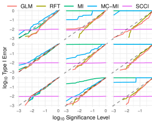
Figure 2: Type I error vs significance level for sample sizes (top to bottom): $[20,40,80]$ and number of conditional variables (left to right): $[1,3,5]$ on conditionally independent simulated binary datasets.

To determine calibration, we analyzed the Type I error rate of the tests at varying significance levels. Under the null $X\perp\!\!\!\!\!\perp Y\mid Z$, for a perfectly calibrated test, we expect the p-value to be uniformly distributed, hence a plot of significance level versus fraction of rejected null hypotheses should be a straight diagonal line. For this analysis, we generated $500$ datasets with all binary variables satisfying the null $X\perp\!\!\!\!\!\perp Y\mid Z$ according to the following structure:

We started by generating uniformly random binary samples $\mathbf{z_{i}}$ for the conditional variables. Then we sampled $\mathbf{x}$ and $\mathbf{y}$ from the binomial distribution $B(2,\mathbf{z_{1}}/3)$. Finally, we computed 500 p-values by testing $X\perp\!\!\!\!\!\perp Y\mid Z$ on each generated dataset using all the tests while varying the number of conditional variables and sample sizes.

Figure 2 shows the results of our analysis on a log-log scale that emphasizes the values in the common range for $p$-value cutoffs. GLM and RFT are better calibrated in most cases except when the number of conditional variables is low with a relatively high sample size (bottom left plot in Figure 2), where MC-MI is better calibrated. Especially for high-dimensional CI tests in small samples, GLM and RFT are much better calibrated compared to the other tests. SCCI is not calibrated at all; this is because it only gives pseudo p-values which are all around $0.01$, with values greater than $0.01$ representing independence.

Discrimination

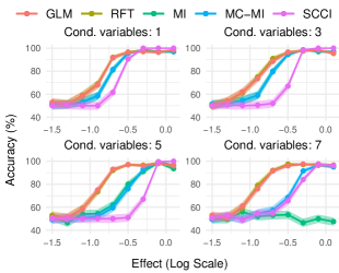
Figure 3: Accuracy (shading: mean $\pm$ standard error, $N=200$) of classifying simulated binary datasets (sample size: $1000$) as conditionally dependent or independent.

Having addressed calibration under null, we now show a discrimination analysis to compare the accuracy of tests on correctly accepting or rejecting the null. We conducted this analysis on both categorical and ordinal data. For deciding between dependence and independence we used a $p$-value threshold of $0.05$ for all tests except SCCI for which we use its designated threshold of $0.01$.

Categorical data.

Our analysis is similar to the one performed by Tsamardinos and Borboudakis (2010). We generated data according to the following general DAG structure:

The $Z_{\geq 2}$ act as irrelevant “nuisance variables”. Our task is to determine whether the edge $X\to Y$ is present (dependent) or absent (independent). We generated binary data using the logistic model

$$p(y_{i}=1)=\lambda(\sum_{X\text{ is a parent of }Y}\beta x_{i})$$ (1)

where $\lambda(x)=e^{x}/(e^{x}+1)$ is the logistic function and $\beta$ is the “effect” (which we fixed to the same value for all edges). Varying the effect and the number of $k$ of conditional variables, we simulated 100 dependent and 100 independent datasets consisting of 1000 samples for each combination.

Figure 3 shows the accuracy of classifying the simulated datasets. All tests perform poorly for tiny effects and strongly for huge effects, but we find that GLM and RFT outperforms the other tests in the “switch regime” in between, with the difference becoming more pronounced when adding nuisance variables. Thus, our test appears to be more robust to noise.

Ordinal data.

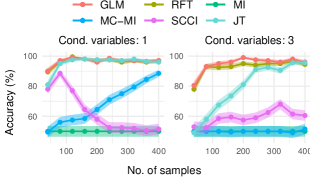
Figure 4: Accuracy (shading: mean $\pm$ standard error, N=200) of classifying simulated ordinal data (8 levels per variable) as conditionally dependent or independent.

We next simulated ordinal data from the same DAG structure as follows: we first generated samples $\mathbf{z_{i}},1\leq i\leq k$ from the binomial distribution $B(8,0.5)$. To generate independent data, we independently sampled $\mathbf{x}$ and $\mathbf{y}$ from $B(8,\frac{\mathbf{z_{1}}}{9})$. To generate dependent data, we then randomly permuted $\mathbf{z_{1}}$. Figure 4 shows the accuracy of the tests computed on $100$ conditionally dependent and independent datasets. In this setup, we varied the sample size rather than an effect size. For $k=1$, GLM, RFT, and JT performed equally well and better than the other tests, which do not take the order of the categories into account. But for $k=3$, GLM and RFT were more accurate than JT in small samples.

Applications

We evaluated our test on two important applications of CI tests: (1) model testing and (2) structure learning. We used the same baselines as in the previous section for comparison.

Model testing

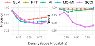
Figure 5: Precision and recall of testing implied versus non-implied CIs in binary data (N=1000) simulated from random DAGs on $20$ variables. Shading: mean $\pm$ standard error.

The CIs implied by a DAG should hold in the dataset(s) it is supposed to represent. Therefore, we can scrutinize a DAG by testing implied CIs. In our analysis, we simulated datasets from randomly generated DAGs and compared how well the tests can correctly detect the implied CIs of the DAG in the simulated dataset. We started by generating random DAGs on $20$ variables. We connected each pair of variables at a fixed probability, with all edges oriented according to a pre-defined topological ordering. We then simulated binary datasets with $1000$ samples using our logistic model (Equation 1) setting $\beta=0.15$. Then we used the CI tests to test one implied CI per missing edge and an equal number of randomly generated CIs in the dataset. For generating a random CI $X\perp\!\!\!\!\!\perp Y\mid Z$, we first selected $X$ and $Y$ variables randomly and then selected a random number of conditional variables $Z$ from the remaining variables. Using d-separation, we determined which randomly generated CIs truly hold in the DAG. All CIs were then tested in the simulated data and precision and recall were computed (Figure 5). The precision of all methods was comparable in sparse DAGs, as the implied CIs had relatively few conditional variables. But in denser DAGs, GLM and RFT had better precision. Recall was comparable for all tests except SCCI, which did not perform well.

Structure learning

CI tests also play an important role in constraint-based structure learning, where algorithms iteratively perform CI tests to determine whether two variables in the model are connected by an edge or not. For learning the network structures in this section, we use the implementation of fast “stable” variant (Colombo and Maathuis 2014) of PC algorithm (Spirtes et al. 2000) from the R package ’pcalg‘ (Kalisch et al. 2012).

Simulated data.

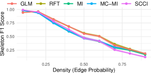
Figure 6: Structure learning on simulated data: Mean F1 scores (10 simulated binary datasets per point) for varying graph densities. Each dataset contains 1000 samples and is simulated from a randomly generated DAG with 20 variables. Shading: mean $\pm$ standard error.

We first show empirical results of structure learning on simulated datasets. We randomly generated DAGs with varying densities as in the previous section. For each DAG, we generated $1000$ samples using our logistic model (Equation 1) using $\beta=0.15$. We used the PC algorithm to learn the model skeleton for each simulated dataset and compared it to the true skeleton using the F1 score (Figure 6). All tests performed comparably for sparse DAGs. For denser DAGs, the stratification tests MI and MC-MI performed the worst, whereas the variable importance test SCCI performed better. Yet GLM and RFT substantially outperformed SCCI, as expected given the results in Figure 3.

Synthetic benchmark data.

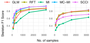
Figure 7: Structure learning on datasets “alarm” (left) and “insurance” (right): Mean F1 scores (10 subsampled datasets per sample size) of the learned model skeletons. Presence of an edge is considered the “positive” case for F1 scores. Shading: mean $\pm$ standard error.

We next evaluated the performance of the tests on two commonly used datasets in structure learning benchmarks, the “alarm” (Beinlich et al. 1989) and “insurance” (Binder et al. 1997) datasets, which again are simulated data from known ground truth. We used the PC algorithm to learn the skeleton using subsampled datasets of varying sizes, and determined F1 scores (Figure 7). SCCI and MC-MI perform best for the alarm model whereas GLM, RFT, and MC-MI perform equally well for the insurance model (except for very low sample size). Importantly, both these models are very sparse. The alarm model has 37 variables and 46 edges, hence the edge probability is $\frac{46}{(37*36)/2}=0.069$. The insurance model is slightly denser with 27 variables and 52 edges and an edge probability of $\frac{52}{(27*26)/2}=0.15$. As PC algorithm removes most of the edges in early iterations (i.e. low conditioning variables) for sparse models, when tests perform poorly in these initial iterations, it can lead to a cascading effect where the algorithm ends up doing many more tests and may reach a higher number of conditioning variables. We saw this happening with GLM and RFT in these datasets as it is slightly less well calibrated than MC-MI for low number of conditional variables and high sample size (Figure 2). Moreover, MC-MI’s bias towards classifying a CI as independent (Figure 2) helps in learning sparser models.

Real data.

(a)

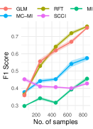
(b)

Figure 8: Structure learning on adult income data. (a) Skeleton estimated by the stable PC algorithm from the data in Figure 1 when using our Random-Forest based test (RFT). (b) Mean F1 score ($10$ adult income data subsamples per point) when comparing $d$-connected variable pairs in the CPDAG to correlated variable pairs in the dataset. Presence of d-connection is used as the positive case for the F1 score. Shading: mean $\pm$ standard error.

Finally, we return to the adult income data. Using PC structure learning with our RFT, a more connected skeleton was generated (Figure 8(a)) compared to the earlier baseline (Figure 1). For systematic quantitative evaluation, we discretized the variable “Age” into the categories $<21$, $21\text{-}30$, $\ldots$, $61\text{-}70$, $>70$ and the variable “HoursPerWeek” into the categories $<=20$, $21\text{-}30$, $30\text{-}40$, $>40$. We then tested whether pairwise dependence in the data corresponded to d-connectedness in learned structures – a reasonable requirement that is evaluable even in the absence of a ground truth structure. To determine pairwise dependences, we performed chi-square independence tests for each variable pair and considered the variables dependent if the root mean square error of approximation, a chi-square effect size defined by $\sqrt{(\chi^{2}-\text{df})/(n\text{df})}$, is greater than $0.05$. We then learned model structures on subsamples of the dataset, and calculated F1 scores by comparing d-connected variables in the learned CPDAG to dependent variables in the dataset. GLM and RFT performed best except for the smallest sample sizes (Figure 8(b)).

Taken together, our results show that our GLM and RFT perform similarly or slightly worse than baselines for low-dimensional, limited data, but equally or better in the other cases. Especially in our motivating scenario of high-dimensional, tightly correlated datasets, the performance gain is substantial. GLM and RFT were slower than most baselines but faster than MC-MI (Figure 9).

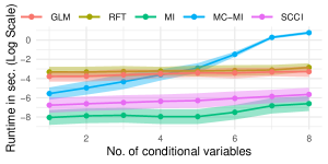
Figure 9: Mean runtime (100 CI tests per point) with varying numbers of conditional variables and $1000$ samples per dataset; data is generated like in Figure 3. Shading: mean $\pm$ standard error.

Conclusion

We have proposed a residualization-based approach for CI testing for discrete and ordinal data. We think this approach could be especially attractive for manual model testing in empirical research because (1) it is symmetric by construction; (2) it is based on rather elementary statistical concepts (here we used Hotelling’s test and GLM/random forest); and (3) its computational cost is reasonable. In addition to these qualitative advantages, we showed that it compares favorably to existing alternatives with respect to calibration, discrimination, and power, and is useful in the context of structure learning when the networks can be expected to be dense, which is the case for many real-world datasets.

Although the test is sensitive to model misspecification when computing the residuals, it provides the flexibility to choose a parametric M-estimator that is suitable for the data at hand. Alternatively, we found the non-parametric Random Forest estimator to perform well empirically.

We have shown that the LS residuals that our approach is based on are closely related to partial copulas. We therefore believe that it should be possible to combine the CI testing approach proposed by Petersen and Hansen (2021) with our approach to obtain a single, unifying CI testing framework for any kind of mixed dataset.

Since our approach outperforms baselines in high- but not low-dimensional settings, structure learning algorithms might be able to get the “best of both worlds” by adaptively choosing our test or a simpler one based on some estimation of how well the simpler test should perform. However, appropriate criteria for switching between the two tests would need to be developed first.

For now, we hope that the combination of our residualization approach and a random forest might be a reasonably robust “plug-in” solution for causal model testing and structure learning in datasets containing ordinal and categorical variables. We hope that this might help to persuade more empirical researchers to test their graphical causal models or to try out structure learning algorithms.

Appendix A Proofs of propositions

For proving the asymptotic distributions of our test statistics under the null, we use the asymptotic distribution proof from Li and Shepherd (2010) as a template and define m-estimators (mestimation) for our test statistics. Given a vector of parameters $\bm{\theta}$ and a function $\Psi_{i}(\bm{\theta})=\Psi(Y_{i},X_{i},\bm{Z}_{i};\bm{\theta})$, such that the following conditions are satisfied:

1. $\bm{\theta}$ can be estimated using $\sum_{i=1}^{n}\Psi_{i}(\bm{\theta})=0$

2. $\Psi_{i}$ doesn’t depend on $i$ or $n$.

3. $\mathbb{E}[\Psi_{i}(\bm{\theta})]=0$

From m-estimation theory, if $\Psi$ is suitably smooth, then as $n\rightarrow\infty$,

$$\sqrt{n}(\hat{\bm{\theta}}-\bm{\theta})\rightarrow\mathcal{N}(0,V(\bm{\theta}))$$ (2)

where $V(\bm{\theta})=A(\bm{\theta})^{-1}B(\bm{\theta})[A(\bm{\theta})^{-1}]^{\prime}$, $A(\bm{\theta})=\mathbb{E}\left[-\frac{\partial}{\partial\bm{\theta}}\Psi_{i}(\bm{\theta})\right]$, and $B(\bm{\theta})=\mathbb{E}[\Psi_{i}(\bm{\theta})\Psi_{i}{\bm{\theta}}]^{\prime}$.

Further, from the delta method, given a function $g(\bm{\theta})$ which is a smooth function of $\bm{\theta}$, we have:

$$\sqrt{n}\left[g(\hat{\bm{\theta}})-g(\bm{\theta})\right]\rightarrow\mathcal{N}(0,\sigma^{2})$$ (3)

where $\sigma^{2}=\left[\frac{\partial}{\partial\bm{\theta}}g(\bm{\theta})\right]V(\bm{\theta})\left[\frac{\partial}{\partial\bm{\theta}}g(\bm{\theta})\right]^{\prime}$

We now define $\bm{\theta}$, $\Psi_{i}$, and $g(\bm{\theta})$ for each of our three test statistics. We separate our parameter vector into three subvectors as $\bm{\theta}=\{\bm{\theta}^{\bm{X}},\bm{\theta}^{\bm{Y}},\bm{\theta}^{\bm{T}}\}$, where $\bm{\theta}^{\bm{X}}$ and $\bm{\theta}^{\bm{Y}}$ are the parameters of the models $P(X|\bm{Z})$ and $P(Y|\bm{Z})$, respectively. Since these parameters and the m-estimator over these parameters are the same for all the test statistics, we first define a partial m-estimator, $\Phi_{i}$ on these parameters.

$$\Phi_{i}(\bm{\theta})=\begin{cases}\frac{\partial}{\partial\bm{\theta}^{\bm{Y}}}l_{Y}(Y_{i},\bm{Z}_{i};\bm{\theta^{Y}})\\ \frac{\partial}{\partial\bm{\theta}^{\bm{X}}}l_{X}(X_{i},\bm{Z}_{i};\bm{\theta^{X}})\\ \end{cases}$$ (4)

where $l_{X}$ and $l_{Y}$ are the log-likelihood functions of the probability models $P(Y|\bm{Z})$ and $P(X|\bm{Z})$ (for example, these could be multinomial models) with parameters $\bm{\theta}^{Y}$ and $\bm{\theta}^{X}$ respectively. In the following sub-sections, we use $\Phi_{i}(\bm{\theta})$ as a partial m-estimator and define the remaining parameters ($\bm{\theta}^{\bm{T}}$), the m-estimator on the remaining parameters ($\Psi_{i}(\bm{\theta}^{\bm{T}})$), and a function ($g(\bm{\theta})$) for each of the test statistics.

Proof for proposition 1

Using the partial m-estimator defined in 4, we now define the remaining parameters $\bm{\theta}^{T}$, m-estimator function on $\bm{\theta}^{T}$, and $g(\bm{\theta})$ for $Q_{1}$.

$$\begin{split}\bm{\theta}^{T}&=(\theta_{1},\theta_{2})\\ \Psi(X_{i},Y_{i},\mathbf{Z}_{i};\bm{\theta}^{T})&=\begin{cases}R_{y_{i}}R_{x_{i}}-\theta_{1}\\ (R_{y_{i}}R_{x_{i}})^{2}-\theta_{2}\end{cases}\\ g(\bm{\theta})&=\frac{\theta_{1}}{\sqrt{\theta_{2}-\theta_{1}^{2}}}\\ \end{split}$$ (5)

Here, we have chosen $g(\bm{\theta})$ such that $Q_{1}=(\sqrt{n}g(\bm{\theta}))^{2}$. Further, solving the equation $\sum_{i}\Psi(X_{i},Y_{i},\mathbf{Z}_{i};\bm{\theta}^{T})=0$ gives us the estimates for $\theta_{1}$ and $\theta_{2}$,

$$\begin{split}\hat{\theta}_{1}&=\mathbb{E}[R_{\mathbf{x}}R_{\mathbf{y}}]\\ \hat{\theta}_{2}&=\mathbb{E}[(R_{\mathbf{x}}R_{\mathbf{y}})^{2}]\\ \end{split}$$ (6)

As both $\Psi$ and $g(\bm{\theta})$ are smooth functions, from m-estimation theory and the delta method as $n\rightarrow\infty$,

$$\sqrt{n}(g(\hat{\bm{\theta}})-g(\bm{\theta}))\rightarrow\mathcal{N}(0,\sigma^{2})$$

Since under the null $g(\bm{\theta})=0$,

$$\sqrt{n}g(\hat{\bm{\theta}})\rightarrow\mathcal{N}(0,\sigma^{2})\\$$ (7)

where $\sigma^{2}$ can be computed as defined in Eq 3.

$$\begin{split}A(\bm{\theta})&=E\left[-\frac{\partial}{\partial\theta_{1}}\Psi_{i}(\bm{\theta}),-\frac{\partial}{\partial\theta_{2}}\Psi_{i}(\bm{\theta})\right]=E\begin{bmatrix}1&0\\ 0&1\end{bmatrix}=\mathbb{I}_{2}\\ B(\bm{\theta})&=\mathbb{E}\begin{bmatrix}(R_{y_{i}}R_{x_{i}}-\theta_{1})(R_{y_{i}}R_{x_{i}}-\theta_{1})&(R_{y_{i}}R_{x_{i}}-\theta_{1})((R_{y_{i}}R_{x_{i}})^{2}-\theta_{2})\\ ((R_{y_{i}}R_{x_{i}})^{2}-\theta_{2})(R_{y_{i}}R_{x_{i}}-\theta_{1})&((R_{y_{i}}R_{x_{i}})^{2}-\theta_{2})((R_{y_{i}}R_{x_{i}})^{2}-\theta_{2})\\ \end{bmatrix}\\ &=\begin{bmatrix}\theta_{2}&\mathbb{E}[(R_{\mathbf{x}}R_{\mathbf{y}})^{3}]\\ \mathbb{E}[(R_{\mathbf{x}}R_{\mathbf{y}})^{3}&\mathbb{E}[(R_{\mathbf{x}}R_{\mathbf{y}})^{4}]-\theta_{2}^{2}\\ \end{bmatrix}\text{(as $\theta_{1}=0$ under the null)}\\ V(\bm{\theta})&=A(\bm{\theta})^{-1}B(\bm{\theta})[A(\bm{\theta})^{-1}]^{\prime}=B(\bm{\theta})\\ \frac{\partial}{\partial\theta}g(\bm{\theta})&=\begin{bmatrix}\frac{\partial}{\partial\theta_{1}}g(\bm{\theta})&\frac{\partial}{\partial\theta_{2}}g(\bm{\theta})\end{bmatrix}=\begin{bmatrix}\theta_{2}^{-\frac{1}{2}}&0\\ \end{bmatrix}\\ \sigma^{2}&=\begin{bmatrix}\theta_{2}^{-\frac{1}{2}}&0\end{bmatrix}\begin{bmatrix}\theta_{2}&\mathbb{E}[(R_{\mathbf{x}}R_{\mathbf{y}})^{3}]\\ \mathbb{E}[(R_{\mathbf{x}}R_{\mathbf{y}})^{3}]&\mathbb{E}[(R_{\mathbf{x}}R_{\mathbf{y}})^{4}]-\theta_{2}^{2}\\ \end{bmatrix}\begin{bmatrix}\theta_{2}^{-\frac{1}{2}}\\ 0\\ \end{bmatrix}\\ &=((\theta_{2})^{-\frac{1}{2}})^{2}\theta_{2}+0+0=1\\ \end{split}$$ (8)

Hence, $\sqrt{n}g(\bm{\theta})$ has an asymptotic standard normal distribution. Since, $Q_{1}=(\sqrt{n}g(\bm{\theta}))^{2}$, $Q_{1}$ is asymptotically chi-square distributed with $1$ degree of freedom.

Proof for proposition 2

Similar to the last proof, we start by defining the remaining parameters, the m-estimator function, and $g(\bm{\theta})$ for $Q_{2}$.

$$\begin{split}&\bm{\theta}^{T}=(\bm{\theta_{1}},\bm{\theta_{2}})\\ &\bm{\theta_{1}}=(\theta_{1}^{1},\theta_{1}^{2},\cdots,\theta_{1}^{k-1})\\ &\bm{\theta_{2}}=(\theta_{2}^{11},\cdots,\theta_{2}^{1(k-1)},\theta_{2}^{21},\cdots,\theta_{2}^{2(k-1)},\cdots,\theta_{2}^{(k-1)(k-1)})\\ &\Psi(X_{i},Y_{i},\mathbf{Z}_{i};\bm{\theta}^{T})=\begin{cases}R_{{\mathbb{I}(x=j)}_{i}}.R_{y_{i}}-\theta_{1}^{j}\,\,\forall j\in\{1,\cdots,k-1\}\\ (R_{{\mathbb{I}(x=j)}_{i}}.R_{y_{i}}\times R_{{\mathbb{I}(x=k)}_{i}}.R_{y_{i}})-\theta_{2}^{jk}\,\,\forall j,k\in\{1,\cdots,k-1\}\\ \end{cases}\\ &g(\bm{\theta})=\bm{\theta_{1}}\bm{\wedge}\end{split}$$ (9)

where $\bm{\wedge}$ is defined as:

$$\begin{split}\bm{\wedge}&=\bm{\Sigma}^{-\frac{1}{2}}\\ \Sigma^{i,j}&=\mathbb{E}[(R_{\mathbb{I}(\mathbf{x}=i)}.R_{\mathbf{y}})(R_{\mathbb{I}(\mathbf{x}=j)}.R_{\mathbf{y}})]-\mathbb{E}[R_{\mathbb{I}(\mathbf{x}=i)}.R_{\mathbf{y}}]\mathbb{E}[R_{\mathbb{I}(\mathbf{x}=j)}.R_{\mathbf{y}}]\\ &=\theta_{2}^{ij}-\theta_{1}^{i}\theta_{1}^{j}\\ \end{split}$$ (10)

Here, we have chosen $g(\bm{\theta})$ such that $Q_{2}=\sum(\sqrt{n}g(\bm{\theta}))^{2}$. Further, solving the equation $\sum_{i}\Psi(X_{i},Y_{i},\mathbf{Z}_{i};\bm{\theta}^{T})=0$ gives us estimates for $\bm{\theta_{1}}$ and $\bm{\theta_{2}}$:

$$\begin{split}\hat{\theta}_{1}^{j}&=\mathbb{E}[R_{\mathbb{I}(\mathbf{x}=j)}R_{\mathbf{y}}]\\ \hat{\theta}_{2}^{jk}&=\mathbb{E}[(R_{\mathbb{I}(\mathbf{x}=j)}R_{\mathbf{y}})(R_{\mathbb{I}(\mathbf{x}=k)}R_{\mathbf{y}})]\\ \end{split}$$ (11)

Similar to the last case as both $\Psi$ and $g(\bm{\theta})$ are smooth functions with $g(\bm{\theta})=0$ under the null,

$$\sqrt{n}g(\hat{\bm{\theta}})\rightarrow\mathcal{N}(\bm{0},\bm{\sigma}^{2})$$

We again use Eq 3 to compute $\bm{\sigma}$ with $A(\bm{\theta})$ defined as,

$$A(\bm{\theta})=\mathbb{E}\left[-\frac{\partial}{\partial\theta_{1}^{j}}\Psi_{i}(\bm{\theta}),-\frac{\partial}{\partial\theta_{2}^{jk}}\Psi_{i}(\bm{\theta})\right]=\mathbb{I}_{k(k-1)}$$ (12)

The matrix $B(\bm{\theta})$ has $4$ types of terms. To simplify the notation, we split $B(\bm{\theta})$ into sub-matrics $\bm{B_{00}}$, $\bm{B_{01}}$, $\bm{B_{10}}$, and $\bm{B_{11}}$ with shapes $(k-1)\times(k-1)$, $(k-1)\times(k-1)^{2}$, $(k-1)^{2}\times(k-1)$, and $(k-1)^{2}\times(k-1)^{2}$ respectively:

$$\begin{split}B(\bm{\theta})&=\begin{bmatrix}\bm{B_{00}}&\bm{B_{01}}\\ \bm{B_{10}}&\bm{B_{11}}\\ \end{bmatrix}\\ B_{00}^{i,j}&=\mathbb{E}[(R_{\mathbb{I}(x=i)}R_{y}-\theta_{1}^{i})(R_{\mathbb{I}(x=j)}R_{y}-\theta_{1}^{j})]\\ &=\theta_{2}^{ij}-2\theta_{1}^{i}\theta_{1}^{j}+\theta_{1}^{i}\theta_{1}^{j}=\theta_{2}^{ij}=\bm{\Sigma}\,\,\text{(as $\bm{\theta_{1}}=0$ under the null)}\\ B_{10}^{i,jk}&=\mathbb{E}[(R_{\mathbb{I}(x=i)}R_{y}-\theta_{1}^{i})(R_{\mathbb{I}(x=j)}R_{y}\times R_{\mathbb{I}(x=k)}R_{y}-\theta_{2}^{jk})]\\ &=\mathbb{E}[R_{\mathbb{I}(x=i)}R_{y}R_{\mathbb{I}(x=j)}R_{y}R_{\mathbb{I}(x=k)}R_{y}]-\theta_{1}^{i}\theta_{2}^{jk}-\theta_{1}^{i}\theta_{2}^{jk}-\theta_{1}^{i}\theta_{2}^{jk}\\ &=\mathbb{E}[R_{\mathbb{I}(x=i)}R_{y}R_{\mathbb{I}(x=j)}R_{y}R_{\mathbb{I}(x=k)}R_{y}]\,\,\text{(as $\bm{\theta_{1}}=0$ under the null)}\\ \bm{B_{01}}&=\bm{B_{10}}^{T}\\ B_{11}^{ij,kl}&=\mathbb{E}[(R_{\mathbb{I}(x=i)}R_{y}R_{\mathbb{I}(x=j)}R_{y}-\theta_{2}^{ij})(R_{\mathbb{I}(x=k)}R_{y}R_{\mathbb{I}(x=l)}R_{y}-\theta_{2}^{kl})]\\ &=\mathbb{E}[(R_{\mathbb{I}(x=i)}R_{y}R_{\mathbb{I}(x=j)}R_{y}R_{\mathbb{I}(x=k)}R_{y}R_{\mathbb{I}(x=l)}R_{y})]-\theta_{2}^{ij}\theta_{2}^{kl}-\theta_{2}^{ij}\theta_{2}^{kl}+\theta_{2}^{ij}\theta_{2}^{kl}\\ &=\mathbb{E}[(R_{\mathbb{I}(x=i)}R_{y}R_{\mathbb{I}(x=j)}R_{y}R_{\mathbb{I}(x=k)}R_{y}R_{\mathbb{I}(x=l)}R_{y})]-\theta_{2}^{ij}\theta_{2}^{kl}\end{split}$$ (13)

Using these terms, we can now compute $\bm{\sigma}$.

$$\begin{split}\frac{\partial}{\partial\theta}g(\bm{\theta})&=\begin{bmatrix}\frac{\partial}{\partial\bm{\theta_{1}}}g(\bm{\theta})&\frac{\partial}{\partial\bm{\theta_{2}}}g(\bm{\theta})\\ \end{bmatrix}\\ \left[\frac{\partial}{\partial\bm{\theta_{1}}}g(\bm{\theta})\right]^{j,l}&=\sum_{p=1}^{k-1}\theta_{1}^{p}\frac{\partial}{\partial\theta_{1}^{j}}\wedge^{p,j}+\wedge^{l,j}=\wedge^{l,j}\\ \left[\frac{\partial}{\partial\bm{\theta_{2}}}g(\bm{\theta})\right]^{j,lm}&=\sum_{p=1}^{k-1}\theta_{1}^{p}\frac{\partial}{\partial\theta_{2}^{lm}}\wedge^{p,j}=0\\ \frac{\partial}{\partial\bm{\theta}}g(\bm{\theta})&=\begin{bmatrix}\bm{\wedge}&\bm{0}\end{bmatrix}\\ \bm{\sigma}^{2}&=\bm{B_{00}}(\bm{\wedge})^{2}=\bm{\Sigma}(\bm{\Sigma}^{-1/2})^{2}=\mathbb{I}_{(k-1)}\end{split}$$ (14)

Hence, $\sqrt{n}g(\bm{\theta})$ has an asymptotic $k-1$ variate standard normal distribution. Since, $Q_{2}=\sum(\sqrt{n}g(\bm{\theta}))^{2}$, $Q_{2}$ is asymptotically chi-square distributed with $k-1$ degrees of freedom.

Proof for proposition 3

The m-estimator for $Q_{3}$ is very similar to $Q_{2}$. We define the parameters, the m-estimator function, and $g(\bm{\theta})$ as:

$$\begin{split}\bm{\theta}^{T}&=(\bm{\theta_{1}},\bm{\theta_{2}})\\ \bm{\theta_{1}}&=(\theta_{1}^{pq})_{p=\{1,\cdots,(k-1)\},q=\{1,\cdots,(r-1)\}}\\ \bm{\theta_{2}}&=(\theta_{2}^{pqst})_{p,s=\{1,\cdots,k-1\},q,t=\{1,\cdots,r-1\}}\\ \Psi(X_{i},Y_{i},\mathbf{Z}_{i};\bm{\theta}^{T})&=\begin{cases}R_{{\mathbb{I}(x=p)}_{i}}.R_{{\mathbb{I}(y=q)}_{i}}-\theta_{1}^{pq}\,\,\forall p\in\{1,\cdots,k-1\},q\in\{1,\cdots,r-1\}\\ (R_{{\mathbb{I}(x=p)}_{i}}.R_{{\mathbb{I}(y=q)}_{i}}\times R_{{\mathbb{I}(x=s)}_{i}}.R_{{\mathbb{I}(y=t)}_{i}})-\theta_{2}^{pqst}\,\,\forall p,s\in\{1,\cdots,k-1\},q,t\in\{1,\cdots,r-1\}\\ \end{cases}\\ g(\bm{\theta})&=\bm{\theta_{1}}\bm{\wedge}\\ \end{split}$$ (15)

where $\bm{\wedge}$ is defined as:

$$\begin{split}\bm{\wedge}&=\bm{\Sigma}^{-1}\\ \Sigma^{ps,qt}&=\mathbb{E}[(R_{\mathbb{I}(x=p)}R_{\mathbb{I}(y=q)})(R_{\mathbb{I}(x=s)}R_{\mathbb{I}(y=t)})]-\mathbb{E}[R_{\mathbb{I}(x=p)}R_{\mathbb{I}(y=q)}]\mathbb{E}[R_{\mathbb{I}(x=s)}R_{\mathbb{I}(y=t)}]\\ &=\theta_{2}^{pqst}-\theta_{1}^{pq}\theta_{1}^{st}\\ \end{split}$$ (16)

Solving the equation $\sum_{i}\Psi(X_{i},Y_{i},\mathbf{Z}_{i};\bm{\theta}^{T})=0$ gives us:

$$\begin{split}\theta_{1}^{pq}&=\mathbb{E}[R_{\mathbb{I}(x=p)}R_{\mathbb{I}(y=q)}]\\ \theta_{2}^{pqst}&=\mathbb{E}[(R_{\mathbb{I}(x=p)}R_{\mathbb{I}(y=q)})(R_{\mathbb{I}(x=s)}R_{\mathbb{I}(y=t)})]\\ \end{split}$$ (17)

Similar to the last case as both $\Psi$ and $g(\bm{\theta})$ are smooth functions with $g(\bm{\theta})=0$ under the null,

$$\sqrt{n}g(\hat{\bm{\theta}})\rightarrow\mathcal{N}(\bm{0},\bm{\sigma}^{2})$$ (18)

The rest of the proof is very similar to the last case and we get the following values for the matrices:

$$\begin{split}A(\bm{\theta})&=\mathbb{I}_{(k-1)(r-1)}\\ B(\bm{\theta})&=\begin{bmatrix}\bm{B_{00}}&\bm{B_{01}}\\ \bm{B_{10}}&\bm{B_{11}}\\ \end{bmatrix}\\ \bm{B_{00}}&=\bm{\Sigma}\\ B_{10}^{lm,stuv}&=\mathbb{E}[R_{\mathbb{I}(x=l)}R_{\mathbb{I}(y=m)}R_{\mathbb{I}(x=s)}R_{\mathbb{I}(y=t)}R_{\mathbb{I}(x=u)}R_{\mathbb{I}(y=v)}]\\ \bm{B_{01}}&=\bm{B_{10}}^{T}\\ B_{11}^{lmpq,stuv}&=\mathbb{E}[(R_{\mathbb{I}(x=l)}R_{\mathbb{I}(y=m)})(R_{\mathbb{I}(x=p)}R_{\mathbb{I}(y=q)})(R_{\mathbb{I}(x=s)}R_{\mathbb{I}(y=t)})(R_{\mathbb{I}(x=u)}R_{\mathbb{I}(y=v)})]-\theta_{2}^{lmpq}\theta_{2}^{stuv}\\ \frac{\partial}{\partial\theta}g(\bm{\theta})&=\begin{bmatrix}\bm{\wedge}&\bm{0}\end{bmatrix}\\ \bm{\sigma}^{2}&=\mathbb{I}_{(k-1)(r-1)}\\ \end{split}$$ (19)

Hence, $\sqrt{n}g(\bm{\theta})$ has an asymptotic $(k-1)(r-1)$ variate standard normal distribution. Since, $Q_{3}=\sum(\sqrt{n}g(\bm{\theta}))^{2}$, $Q_{3}$ is asymptotically chi-square distributed with $(k-1)(r-1)$ degrees of freedom.

References

- Beinlich et al. (1989) Beinlich, I. A.; Suermondt, H. J.; Chavez, R. M.; and Cooper, G. F. 1989. The ALARM Monitoring System: A Case Study with two Probabilistic Inference Techniques for Belief Networks. In Hunter, J.; Cookson, J.; and Wyatt, J., eds., AIME 89, 247–256. Springer. ISBN 978-3-642-93437-7.
- Bergsma (2004) Bergsma, W. P. 2004. Testing conditional independence for continuous random variables. Technical Report 2004-049, EURANDOM.
- Berrett and Samworth (2019) Berrett, T. B.; and Samworth, R. J. 2019. Nonparametric independence testing via mutual information. Biometrika, 106(3): 547–566.
- Binder et al. (1997) Binder, J.; Koller, D.; Russell, S.; and Kanazawa, K. 1997. Adaptive probabilistic networks with hidden variables. Machine Learning, 29(2): 213–244.
- Colombo and Maathuis (2014) Colombo, D.; and Maathuis, M. H. 2014. Order-Independent Constraint-Based Causal Structure Learning. Journal of Machine Learning Research, 15: 3921–3962.
- Cover (1999) Cover, T. M. 1999. Elements of information theory. John Wiley & Sons. ISBN 978-0-471-24195-9.
- Daudin (1980) Daudin, J. J. 1980. Partial association measures and an application to qualitative regression. Biometrika, 67(3): 581–590.
- Dawid (1979) Dawid, A. P. 1979. Conditional Independence in Statistical Theory. Journal of the Royal Statistical Society. Series B (Methodological), 41(1): 1–31.
- Dua and Graff (2017) Dua, D.; and Graff, C. 2017. UCI Machine Learning Repository.
- Edwards (2012) Edwards, D. 2012. Introduction to graphical modelling. Springer. ISBN 978-0-387-95054-9.
- Gretton et al. (2005) Gretton, A.; Bousquet, O.; Smola, A.; and Schölkopf, B. 2005. Measuring Statistical Dependence with Hilbert-Schmidt Norms. In Jain, S.; Simon, H. U.; and Tomita, E., eds., Algorithmic Learning Theory, 63–77. Springer. ISBN 978-3-540-31696-1.
- Heinze-Deml, Peters, and Meinshausen (2018) Heinze-Deml, C.; Peters, J.; and Meinshausen, N. 2018. Invariant Causal Prediction for Nonlinear Models. Journal of Causal Inference, 6(2).
- Jonckheere (1954) Jonckheere, A. R. 1954. A Distribution-Free k-Sample Test Against Ordered Alternatives. Biometrika, 41(1/2): 133–145.
- Josse and Holmes (2014) Josse, J.; and Holmes, S. 2014. Measures of dependence between random vectors and tests of independence. Literature review. arXiv:1307.7383.
- Kalisch et al. (2012) Kalisch, M.; Mächler, M.; Colombo, D.; Maathuis, M. H.; and Bühlmann, P. 2012. Causal Inference Using Graphical Models with the R Package pcalg. Journal of Statistical Software, 47(11): 1–26.
- Kohavi (1996) Kohavi, R. 1996. Scaling up the Accuracy of Naive-Bayes Classifiers: A Decision-Tree Hybrid. In Proceedings of the Second International Conference on Knowledge Discovery and Data Mining, KDD’96, 202–207. AAAI Press.
- Kojadinovic and Holmes (2009) Kojadinovic, I.; and Holmes, M. 2009. Tests of independence among continuous random vectors based on Cramér–von Mises functionals of the empirical copula process. Journal of Multivariate Analysis, 100(6): 1137–1154.
- Li and Shepherd (2010) Li, C.; and Shepherd, B. E. 2010. Test of Association Between Two Ordinal Variables While Adjusting for Covariates. Journal of the American Statistical Association, 105(490): 612–620.
- Li and Shepherd (2012) Li, C.; and Shepherd, B. E. 2012. A new residual for ordinal outcomes. Biometrika, 99(2): 473–480.
- Malley et al. (2012) Malley, J. D.; Kruppa, J.; Dasgupta, A.; Malley, K. G.; and Ziegler, A. 2012. Probability Machines. Methods of Information in Medicine, 51(01): 74–81.
- Marx and Vreeken (2019) Marx, A.; and Vreeken, J. 2019. Testing Conditional Independence on Discrete Data using Stochastic Complexity. volume 89, 496–505. PMLR.