Optimizing local Hamiltonians for the best metrological performance

Abstract

We discuss efficient methods to optimize the metrological performance over local Hamiltonians in a bipartite quantum system. For a given quantum state, our methods find the best local Hamiltonian for which the state outperforms separable states the most from the point of view of quantum metrology. We show that this problem can be reduced to maximize the quantum Fisher information over a certain set of Hamiltonians. We present the quantum Fisher information in a bilinear form and maximize it by iterating a see-saw, in which each step is based on semidefinite programming. We also solve the problem with the method of moments that works very well for smaller systems. We consider a number of other problems in quantum information theory that can be solved in a similar manner. For instance, we determine the bound entangled quantum states that maximally violate the Computable Cross Norm-Realignment (CNNR) criterion.

I Introduction

Quantum entanglement is at the heart of quantum physics and several quantum information processing applications [1, 2, 3, 4]. It also plays a central role in quantum metrology. It is known that interparticle entanglement is needed to overcome the shot-noise limit of the precision in parameter estimation in a linear interferometer [5]. It has also been shown that the larger the achieved precision in parameter estimation with a multiparticle system, the larger the depth of entanglement the state must posses [6, 7]. However, not all entangled states are useful for metrology [8].

At this point, several important questions arise. First, how could we find the quantum state within a given set of states that overcomes the most the performance of separable states for a given Hamiltonian? Efficient iterative methods have been presented for this task for various situations [9, 10, 11, 12]. A variational technique for efficiently searching in the high-dimensional space of quantum states was also applied for a similar task [13].

Another relevant question is how we could find the optimal Hamiltonian for a given quantum state. In the qubit case, it has been studied how to optimize the metrological performance for local Hamiltonians that are all Pauli spin matrices rotated by some unitary [8]. In this case, the best metrological performance achievable by separable states is a constant independent of the Hamiltonian. Any state that has a better metrological performance than that must be entangled.

The problem of the metrological performance of a bipartite state of qudits with a dimension larger than two is more complicated. In this case, the local Hamiltonians cannot be transformed into each other by local unitaries, and the best metrological performance achievable by separable states depends on the Hamiltonian. The metrological gain can be used in this case to characterize the quantum advantage of the system, which is defined as the ratio of the quantum Fisher information and the maximum of the quantum Fisher information over separable states maximized over local Hamiltonians [14]. The metrological gain is convex in the state, and it cannot decrease if additional copies or ancilla systems are added [14]. Note that the quantum Fisher information can be compared to other bounds that are state dependent. This way one can also get quantities that are positive only if the state is entangled [15, 16, 17].

In this paper, we examine the optimization problem above in a great depth. We elaborate the point that local Hamiltonians with meaningful constraints form a convex set. Thus, we have to maximize the metrological gain over a convex set of local Hamiltonians. We find several algorithms to maximize the metrological gain. The first method is based on maximizing a quadratic expression using a see-saw over a bilinear expression, and its computational costs are minimal. We present other algorithms that need quadratic programming with quadratic constraints and relaxations. Such methods work for small systems. We test the methods and compare them to each other. We list a number of similar problems that can be solved in an analogous way, such as maximization of norms over a convex set.

Our work has a relation to resource theories, in which the quantum Fisher information can be used to identify quantum resources [18, 19]. Indeed, quantum Fisher information can be ideal to characterize quantum systems realized in Noisy Intermediate-Scale Quantum Applications [20]. For a resource theory, we need to identify a convex set of free quantum states and a set of free operations. In our case, the free states are the separable states and the free operations include the local unitary operations. We can use the robustness of metrological usefulness defined in Ref. [11] to quantify our resource. It asks the question, how much noise can be added to the state such that it is not useful any more metrologically. In this paper, we will examine another measure, the metrological gain mentioned above.

Our work is also related to recent efforts to solve various problems of numerical optimization in quantum metrology including multiparameter estimation [21, 22, 23, 24, 25, 26]. While several methods optimize over the precision of the parameter estimation and allow for a noisy dynamics, we restrict ourselves to maximize the quantum Fisher information and consider unitary dynamics.

Finally, our work is relevant for the field that attempts to find a quantum advantage in experiments [27, 28, 29, 30]. The bound for quantum Fisher information for separable states has already been used to detect metrologically useful multipartite entanglement in several experiments [31, 32, 33].

Our paper is organized as follows. In Sec. II, we review the basic notions of entanglement theory and quantum metrology. In Sec. III we discuss, how our optimization problem can be viewed as maximization over a convex set of Hamiltonians. We review the notion of metrological gain. In Sec. IV, we present various methods to optimize the quantum Fisher information over a local Hamiltonian. In Sec. V, we consider optimization problems in quantum information that can be solved in a similar way. For instance, we determine the bound entangled quantum states that maximally violate the Computable Cross Norm-Realignment (CNNR) criterion for entanglement detection [34, 35].

II Background

In this section, we review entanglement theory and quantum metrology.

II.1 Entanglement theory

In this section, we summarize basic notions of entanglement theory [1, 2]. A bipartite quantum state is called separable if it can be written as mixture of product states as [36]

$$\varrho_{\rm sep}=\sum_{k}p_{k}\varrho^{(k)}_{1}\otimes\varrho^{(k)}_{2},$$ (1)

where $p_{k}$ are probabilities. If a quantum state cannot be decomposed as in Eq. (1), then the state is entangled.

Deciding whether a quantum state is entangled is a hard task in general. However, there are some necessary conditions for separability, that are easy to test. If these conditions are violated then the state is entangled.

One of the most important conditions of this type is the condition based on the positivity of the partial transpose (PPT). For a bipartite density matrix given as

$$\varrho=\sum_{kl,mn}\varrho_{kl,mn}|k\rangle\langle l|\otimes|m\rangle\langle n|$$ (2)

the partial transpose according to first subsystem is defined by exchanging subscripts $k$ and $l$ as

$$\varrho^{T1}=\sum_{kl,mn}\varrho_{lk,mn}|k\rangle\langle l|\otimes|m\rangle\langle n|.$$ (3)

It has been shown that for separable quantum states [37, 38]

$$\varrho^{T1}\geq 0$$ (4)

holds. Thus, if $\varrho^{T1}$ has a negative eigenvalue then the quantum state is entangled. For $2\times 2$ and $2\times 3$ systems, the PPT condition detects all entangled states [38]. For systems of size $3\times 3$ and larger, there are PPT entangled states [39, 40]. They are also quantum states that are called bound entangled since their entanglement cannot be distilled to singlet states with local operations and classical communication (LOCC). Some of the bound entangled states are detected as entangled by the CCNR criterion [34, 35].

II.2 Quantum metrology

In this section, we summarize basic notions of quantum metrology.

The metrological precision in estimating $\theta$ in a unitary dynamics

$$U_{\theta}=\exp(-iH\theta)$$ (5)

is bounded by the Cramér-Rao bound [41, 42, 43, 44, 45, 46, 47, 48, 49, 50, 51]

$$(\Delta\theta)^{2}\geq\frac{1}{\nu\mathcal{F}_{Q}[\varrho,H]},$$ (6)

where $\nu$ is the number of independent repetitions, $\varrho$ is the density matrix we use for quantum metrology and $H$ is the Hamiltonian of the evolution. Let us consider a density matrix with the following eigendecomposition

$$\varrho=\sum_{k}\lambda_{k}|k\rangle\langle k|.$$ (7)

Then, the quantum Fisher information is defined as [41, 42, 43, 44, 45]

$$\mathcal{F}_{Q}[\varrho,H]=\sum_{k,l}Q_{kl}^{2}|H_{kl}|^{2},$$ (8)

where the constant coefficient is given as

$$Q_{kl}:=\sqrt{2\frac{(\lambda_{k}-\lambda_{l})^{2}}{\lambda_{k}+\lambda_{l}}},$$ (9)

and the matrix element of the Hamiltonian in the basis of the eigenvectors of the density matrix is given as

$$H_{kl}=\langle k|H|l\rangle.$$ (10)

The quantum Fisher information in Eq. (8) can be further written as

$$\mathcal{F}_{Q}[\varrho,H] = \sum_{kl}Q_{kl}^{2}\left[(H_{kl}^{\rm{r}})^{2}+(H_{kl}^{\rm{i}})^{2}\right],$$ (11)

where the superscripts "r" and "i" denote the real and imaginary parts, respectively.

It is useful to stress the basic properties of the quantum Fisher information, namely, that it is convex in the state, and

$$\mathcal{F}_{Q}[\varrho,H]\leq 4(\Delta H)^{2},$$ (12)

where for pure states there is an equality in Eq. (12).

Finally, there is an important inequality for the quantum Fisher information [52, 53, 54]

$$(\Delta\theta)^{2}_{M}\geq\frac{1}{\mathcal{F}_{Q}[\varrho,H]},$$ (13)

where the error propagation formula is defined as

$$(\Delta\theta)^{2}_{M}=\frac{(\Delta M)^{2}}{\langle{i[M,H]}\rangle^{2}}.$$ (14)

$(\Delta\theta)^{2}_{M}$ is the smallest, and thus the bound in Eq. (13) is the best if we choose $M$ to be the symmetric logarithmic derivative

$$M=2i\sum_{k,l}\frac{\lambda_{k}-\lambda_{l}}{\lambda_{k}+\lambda_{l}}|k\rangle\langle l|\langle k|H|l\rangle.$$ (15)

Let us consider the case of several parameters. In this case the unitary dynamics is given by

$$\exp\left(-i\sum_{n}H^{(n)}\theta^{(n)}\right),$$ (16)

where $H^{(n)}$ is the Hamiltonian corresponding to the parameter $\theta^{(n)}.$ The Cramér-Rao bound can be generalized to this case as

$$C-\nu^{-1}F^{-1}\geq 0,$$ (17)

where the inequality in Eq. (17) means that the left-hand side is a positive semidefinite matrix, $C$ is now the covariance matrix with elements

$$C_{mn}=\langle{\theta^{(m)}\theta^{(n)}}\rangle-\langle{\theta^{(m)}}\rangle\langle{\theta^{(n)}}\rangle,$$ (18)

and $F$ is the Fisher matrix, and its elements are given as

$$F_{mn} \equiv \mathcal{F}_{Q}[\varrho,H^{(m)},H^{(n)}].$$ (19)

Here, the quantum Fisher information with two operators is given as

$$\mathcal{F}_{Q}[\varrho,A,B]=\sum_{k,l}Q_{kl}^{2}A_{kl}B_{kl}^{*}\equiv{\rm Tr}[(Q\circ Q\circ A)B],$$ (20)

where $\circ$ is elementwise or Hadamard product. After straightforward algebra, the following equivalent formulation can be obtained

$$\mathcal{F}_{Q}[\varrho,A,B]=\sum_{kl}Q_{kl}^{2}\bigg{[}A_{kl}^{\rm{r}}B_{kl}^{\rm{r}}+A_{kl}^{\rm{i}}B_{kl}^{\rm{i}}\bigg{]}.$$ (21)

If $\varrho$ has low rank, then, based on Eq. (9), $Q$ has many zero elements that can simplify the calculation of Eq. (21).

III Basic notions for optimizing the metrological performance

When maximizing the quantum metrological performance over a Hamiltonian, we have to consider two important issues.

First, not all Hamiltonians are easy to realize. In particular, local Hamiltonians are much easier to realize than Hamiltonians with an interaction term, and such Hamiltonians appear most typically in quantum metrology. Thus, we will restrict the optimization for such Hamiltonians given as

$${\mathcal{H}}=H_{1}\otimes\openone_{2}+\openone_{1}\otimes H_{2},$$ (22)

where $H_{n}$ are single-subsystem operators. In the rest of the paper, ${\mathcal{H}}$ will denote such local Hamiltonians. Moreover, we will use $\mathcal{L}$ to denote the set of local Hamiltonians.

Second, we have to note that for the quantum Fisher information

$$\mathcal{F}_{Q}[\varrho,cH]=|c|^{2}\mathcal{F}_{Q}[\varrho,H]$$ (23)

holds, where $c$ is some constant. Thus, it is easy to improve the metrological performance of any Hamiltonian by multiplying it by a constant factor. In order to obtain a meaningful optimization problem, we have to consider a formulation of such a problem where such a "trick" cannot be used to increase the quantum Fisher information to infinity. One option could be to divide the quantum Fisher information with the square of some norm or seminorm of the Hamiltonian, for which

$$||cH||=|c|\cdot||H||.$$ (24)

In principle, the Hilbert-Schmidt norm

$$||X||_{\rm HS}=\sqrt{{\rm Tr}(XX^{\dagger})}$$ (25)

could be used for the normalization. Arguably, it is natural to compare the metrological performance of a state to the best performance of separable states. We divide the quantum Fisher information of the state by the maximum quantum Fisher information achievable by separable states given as for some $\mathcal{H}\in\mathcal{L}$ as [55, 11]

$$\mathcal{F}_{Q}^{({\rm sep})}(\mathcal{H})=\sum_{n=1,2}[\sigma_{\max}(H_{n})-\sigma_{\min}(H_{n})]^{2},$$ (26)

where $\sigma_{\max}(X)$ and $\sigma_{\min}(X)$ denotes the maximal and minimal eigenvalues, respectively.

III.1 Seminorm for local Hamiltonians

Let us now present the details of our aguments. We will examine some properties of Eq. (26). Let us consider first the quantity

$$\delta(X)=\sigma_{\max}(X)-\sigma_{\min}(X),$$ (27)

where $\sigma_{\min}(X)$ and $\sigma_{\max}(X)$ denote the smallest and largest eigenvalues of $X.$ Simple algebra shows that [56, *[InequalitiessimilartoEq.\eqref{eq:fqdelta}, alsoinvolvingthepurityofthestateandthevariance, canbefoundat][]Toth2017Lower]

$$\mathcal{F}_{Q}[\varrho,X]\leq\delta^{2}(X).$$ (28)

With Eq. (27), the maximum of the quantum Fisher information for separable states, $\mathcal{F}_{Q}^{({\rm sep})},$ can be expressed as

$$\mathcal{F}_{Q}^{({\rm sep})}(\mathcal{H})\equiv\delta^{2}(H_{1})+\delta^{2}(H_{2}).$$ (29)

Next, let us prove some important properties of $\delta(X).$

Observation 1. We know that $\delta(X)$ is a seminorm. While this is shown in Ref. [56], for completeness and since the steps of the proof will be needed later, we present a brief argument to prove it.

Proof. We need the well-known fact that for Hermitian matrices $A$ and $B$

$$\sigma_{\rm max}(A+B) \leq \sigma_{\rm max}(A)+\sigma_{\rm max}(B),$$

$$\sigma_{\rm min}(A+B) \geq \sigma_{\rm min}(A)+\sigma_{\rm min}(B),$$ (30)

holds. Based on these, we will now show that $\delta(X)$ has all the properties of a seminorm [58, 59]. (1) Subadditivity or the triangle inequality holds since

$$\delta(A+B)\leq\delta(A)+\delta(B)$$ (31)

for all $A,B$ based on Eq. (30). (2) Absolute homogeneity holds since

$$\delta(cX)=|c|\delta(X)$$ (32)

for all $c$ and $X.$ (3) Non-negativity holds since $\delta(X)\geq 0$ holds for all $X.$ If $X$ is a zero matrix then $\delta(X)=0.$ However, $\delta(X)=0$ does not imply that $X$ is a zero matrix, thus $\delta(X)$ is not a norm, only a seminorm [58, 59]. $\hfill\blacksquare$

Next, let us prove some important properties of the maximal quantum Fisher information for separable states.

Observation 2. The expression

$$\sqrt{\mathcal{F}_{Q}^{({\rm sep})}(\mathcal{H})}$$ (33)

is a seminorm for $\mathcal{H}\in\mathcal{L}.$

Proof. (i) Let us consider a local Hamiltonian that is the sum of two local Hamiltonians

$$\mathcal{H}=\mathcal{H}^{\prime}+\mathcal{H}^{\prime\prime},$$ (34)

where the two local Hamiltonians are given as

$${\mathcal{H}}^{\prime} = H_{1}^{\prime}\otimes\openone_{2}+\openone_{1}\otimes H_{2}^{\prime},$$

$${\mathcal{H}}^{\prime\prime} = H_{1}^{\prime\prime}\otimes\openone_{2}+\openone_{1}\otimes H_{2}^{\prime\prime}.$$ (35)

Then, the following series of inequalities prove the subadditivity property

$$\quad\sqrt{\delta^{2}(H_{1}^{\prime}+H_{1}^{\prime\prime})+\delta^{2}(H_{2}^{\prime}+H_{2}^{\prime\prime})}$$

$$\quad\leq\sqrt{[\delta(H_{1}^{\prime})+\delta(H_{1}^{\prime\prime})]^{2}+[\delta(H_{2}^{\prime})+\delta(H_{2}^{\prime\prime})]^{2}}$$

$$\quad\leq\sqrt{\delta^{2}(H_{1}^{\prime})+\delta^{2}(H_{1}^{\prime\prime})}+\sqrt{\delta^{2}(H_{2}^{\prime})+\delta^{2}(H_{2}^{\prime\prime})}.$$ (36)

The first inequality in Eq. (36) is due to the subadditivity of $\delta(X)$ and the monotonicity of $\sqrt{x^{2}+y^{2}}$ in $x$ and $y.$ The second inequality is due to the subadditivity of $\sqrt{x^{2}+y^{2}}.$

(ii) Absolute homogeneity,

$$\sqrt{\mathcal{F}_{Q}^{({\rm sep})}(c\mathcal{H})}=|c|\sqrt{\mathcal{F}_{Q}^{({\rm sep})}(\mathcal{H})}$$ (37)

for any real $c$ follows directly from its expression with $\delta(H_{n})$. (iii) Non-negativity is trivial. $\hfill\blacksquare$

Note that $\mathcal{F}_{Q}^{({\rm sep})}(\mathcal{H})=0$ holds if and only if $\mathcal{H}=c\openone,$ where $c$ is a real constant. Thus, in a certain sense, $\mathcal{F}_{Q}^{({\rm sep})}(\mathcal{H}^{\prime}-\mathcal{H}^{\prime\prime})$ plays a role of distance between local Hamiltonians $\mathcal{H}^{\prime}$ and $\mathcal{H}^{\prime\prime}$ such that the distance is zero if $\mathcal{H}^{\prime}-\mathcal{H}^{\prime\prime}$ is the identity times some constant. In this case, the two matrices are not identical, but from the point of view of quantum metrology they act the same way.

Let us see some consequences of the observation. As any seminorm, $\sqrt{\mathcal{F}_{Q}^{({\rm sep})}(\mathcal{H})}$ is convex in the local Hamiltonian. Due to that, $\mathcal{F}_{Q}^{({\rm sep})}(\mathcal{H})$ is also convex.

III.2 Metrological gain

Based on these ideas, we define the metrological gain for a given local Hamiltonian $\mathcal{H}\in\mathcal{L}$ and for a given quantum state as [14]

$$g_{\mathcal{H}}(\varrho)=\frac{\mathcal{F}_{Q}[\varrho,\mathcal{H}]}{\mathcal{F}_{Q}^{({\rm sep})}(\mathcal{H})}.$$ (38)

In Eq. (38), we normalize the quantum Fisher information with a square of a seminorm of local Hamiltonians. Then, we would like to obtain

$$g(\varrho)=\max_{\mathcal{H}\in\mathcal{L}}g_{\mathcal{H}}(\varrho).$$ (39)

Maximizing $g_{\mathcal{H}}$ over $\mathcal{H}$ is difficult since both the numerator and denominator depend on $\mathcal{H}.$ Let us consider a subset of Hamiltonians of the type Eq. (22) such that

$$\sigma_{\min}(H_{n}) = -c_{n},$$

$$\sigma_{\max}(H_{n}) = +c_{n}$$ (40)

for $n=1,2.$ Then,

$$\mathcal{F}_{Q}^{({\rm sep})}(\mathcal{H})=4(c_{1}^{2}+c_{2}^{2}).$$ (41)

We can define the metrological gain for Hamiltonians that fulfill Eq. (40) as

$$g_{c_{1},c_{2}}(\varrho)=\max_{\mathcal{H}\in\mathcal{L}_{c_{1},c_{2}}}\frac{\mathcal{F}_{Q}[\varrho,\mathcal{H}]}{4(c_{1}^{2}+c_{2}^{2})},$$ (42)

where we call $\mathcal{L}_{c_{1},c_{2}}$ the set of local Hamiltonians fulfilling Eq. (40). Finally, the maximal gain is given as

$$g(\varrho)=\max_{c_{1},c_{2}}g_{c_{1},c_{2}}.$$ (43)

Note that $g(\varrho)$ is convex in $\varrho$ [14].

Based on Eq. (42), we can see that computing $g_{c_{1},c_{2}}(\varrho)$ is the same as maximizing the quantum Fisher information for the given set of Hamiltonians. We can do that by requiring that

$$c_{n}\mathbbm{1}\pm H_{n}\geq 0,$$ (44)

where $n=1,2$ and $c_{n}>0$ is some constant. This way we make sure that

$$\sigma_{\min}(H_{n})\geq-c_{n},\quad\sigma_{\max}(H_{n})\leq+c_{n},$$ (45)

for $n=1,2.$ Since we maximize a convex function over a convex set, the optimum is taken on the boundary of the set where the eigenvalues of $H_{n}$ are $\pm c_{n}.$ In this case, $H_{n}^{2}=c_{n}^{2}\openone.$

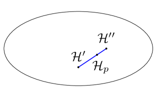
Figure 1: The convex set of local Hamiltonians fulfilling Eq. (44). $\mathcal{H}_{p}$ is given by Eq. (46).

Note that the constrains in Eq. (44) determine a convex set of Hamiltonians. That is, if two Hamiltonians, $\mathcal{H}^{\prime}$ and $\mathcal{H}^{\prime\prime}$, are of the form Eq. (22) with the constraints given in Eq. (44), then their convex combination, i.e.,

$$\mathcal{H}_{p}=p\mathcal{H}^{\prime}+(1-p)\mathcal{H}^{\prime\prime}$$ (46)

with $0\leq p\leq 1$ is also of that form, as shown in Fig. 1. This can be seen based on Eq. (30).

Thus, we need to deal with convex sets, similarly, as convex sets appear in the separability problem of quantum states [36, 1]. In Appendix A, in order to understand better the role of convexity in this case, we define a subset of separable quantum states similar to the local Hamiltonians we consider in this paper.

IV Method for maximizing the quantum Fisher information over local Hamiltonians

In the previous section, we have shown that maximizing the metrological gain is essentially reduced to maximizing the quantum Fisher information with some constraints on the local Hamiltonian given in Eq. (44), that is, computing

$$\max_{\mathcal{H}\in\mathcal{L}_{c_{1},c_{2}}}\mathcal{F}_{Q}[\varrho,\mathcal{H}],$$ (47)

where we remember that $\mathcal{L}_{c_{1},c_{2}}$ is the set of local Hamiltonians fulfilling Eq. (40). Thus, in this section we will present methods that can maximize the quantum Fisher information with such constraints.

IV.1 See-saw optimization based on a bilinear form

In Ref. [14], a method was presented to maximize the quantum Fisher information over local Hamiltonians for a given quantum state. It is an iterative method, that needs to compute the symmetric logarithmic derivative Eq. (15) at each step and is based on quantum metrological considerations. In this section, we will present a simpler formulation based on general ideas in optimization theory. Later, this will also make it possible also to find provably the global maximum of the quantum Fisher information.

The quantum Fisher information given in Eq. (11) is a weighted sum of squares of the elements of the Hamiltonian. It can further be written as

$$\vec{v}^{T}R\vec{v},$$ (48)

where $R$ contains the $Q_{kl}$’s and $\vec{v}$ contains the $H_{kl}^{\rm{r}}$’s and the $H_{kl}^{\rm{i}}$’s. The matrix $R$ is a positive semidefinite diagonal matrix. A usual way of maximizing such an expression is as follows [60, 61, 62]. We replace the optimization by $\vec{v}$ by a simultaneous optimization by the vectors $\vec{v}$ and $\vec{w}$ of a bilinear form as

$$\max_{\vec{v}}\vec{v}^{T}R\vec{v}=\max_{\vec{v},\vec{w}}\vec{v}^{T}R\vec{w}.$$ (49)

This can be a basis for a see-saw-type optimization.

Based on this, we can write the following.

Observation 3. The quantum Fisher information can be maximized with a see-saw method. We need to use the formula maximizing over local Hamiltonians

$$\max_{\mathcal{H}\in\mathcal{L}_{c_{1},c_{2}}}\mathcal{F}_{Q}[\varrho,\mathcal{H}]$$

$$\quad\quad=\max_{\mathcal{H},\mathcal{K}\in\mathcal{L}_{c_{1},c_{2}}}\sum_{kl}Q_{kl}^{2}\bigg{[}\mathcal{H}_{kl}^{\rm{r}}\mathcal{K}_{kl}^{\rm{r}}+\mathcal{H}_{kl}^{\rm{i}}\mathcal{K}_{kl}^{\rm{i}}\bigg{]}$$

$$\quad\quad\equiv\max_{\mathcal{H},\mathcal{K}\in\mathcal{L}_{c_{1},c_{2}}}{\rm Tr}[(Q\circ Q\circ\mathcal{H})\mathcal{K}],$$ (50)

Based on Eq. (50), we can carry out the following algorithm. Initially, we chose $\mathcal{H}$ randomly. Then, we maximize over the matrix $\mathcal{K}$ while keeping $\mathcal{H}$ fixed. Such an optimization can be carried out, for instance, by semidefinite programming [63] or by simple matrix algebraic calculations, see Appendix B. Then, we maximize over $\mathcal{H}$ while keeping $\mathcal{K}$ fixed. Then, we optimize again over $\mathcal{K}$, etc. Note that we do not have to verify that the random initial Hamiltonian fulfills the constraints Eq. (44), since a random initial Hamiltonian $\mathcal{H}$ and $c\mathcal{H}$ for any $c>0$ as initial Hamiltonian will lead to the same optimal $\mathcal{K}.$ (An alternative formulation of the optimization problem is in Appendix C. With similar methods, we also analyze the optimization over a quantum state rather than over the Hamiltonian Appendix D.)

Based on Eq. (21), we can see that Eq. (50) can be expressed as

$$\max_{\mathcal{H}\in\mathcal{L}_{c_{1},c_{2}}}\mathcal{F}_{Q}[\varrho,\mathcal{H}]=\max_{\mathcal{H},\mathcal{K}\in\mathcal{L}_{c_{1},c_{2}}}\mathcal{F}_{Q}[\varrho,\mathcal{H},\mathcal{K}].$$ (51)

This gives a meaningful physical interpretation of the see-saw method.

Since $\mathcal{F}_{Q}[\varrho,H]$ is convex in $H_{kl}^{\rm{r}}$ and $H_{kl}^{\rm{i}},$ if we maximize it over a convex set of Hamiltonians, then it will take the maximum at the boundary of the set. This optimization is a hard task. We have to start from several random initial conditions, and only some of them will find a solution.

We tested our method, together with the method of Ref. [14]. We used MATLAB [64] and semidefinite programming using MOSEK [65] and the YALMIP package [66]. We also used the QUBIT4MATLAB package [67, 68].

	$\mathop{\rm max}F_{Q}[\varrho,H]$				$\mathop{\rm max}4I_{\varrho}$
Quantum state	Dim.	See-saw	Level $1$	Level $2$	See-saw	Level $1$	Level $2$
$\varrho_{AB}^{(0.1,2)}$ from Eq. (52)	2	13.6421	13.6421	13.6421	10.3338	10.3338	10.3338
$\varrho_{AB}^{(0.1,3)}\otimes\varrho_{A^{\prime}B^{\prime}}^{(0.1,3)}$	9	13.8828	14.0568	-	13.4330	13.6009	-
Horodecki, $a=0.3$ [40]	3	4.8859	5.1280	4.8859	4.8020	4.9910	4.8020
UPB [69, 70]	3	5.6913	6.1667	5.6913	5.6913	6.1667	5.6913
Met. useful  PPT [11]	4	9.3726	9.3726	-	9.3726	9.3726	-
Private PPT [71, 12]	6	10.1436	10.1436	-	10.1436	10.1436	-

Table 1: Maximum of the quantum Fisher information and the Wigner-Yanase skew information with the see-saw method for $c_{1}=c_{2}=1$ for various quantum states described in the text. The results for quadratic programming for various levels of approximation are also shown. "Met. useful PPT" denotes the metrologically useful PPT state considered in Ref. [11], whereas "Private PPT" denotes the PPT state based on private states given in Refs. [71, 12].

We tested our method for a number of quantum states. We considered the isotropic state of two $d$-dimensional qudits defined as

$$\varrho_{AB}^{(p,d)}=(1-p)|\Psi_{\rm me}\rangle\langle\Psi_{\rm me}|+p\frac{\openone}{d^{2}},$$ (52)

where $|\Psi_{\rm me}\rangle$ is the maximally entangled state and $p$ is the fraction of the white noise. In particular, we considered $p=0.1$ and $d=2$. For such states, the optimal Hamiltonian is known analytically [14]. We also considered two copies of the state $p=0.1$ and $d=3$ given as $\varrho_{AB}^{(0.1,3)}\otimes\varrho_{A^{\prime}B^{\prime}}^{(0.1,3)},$ where the bipartite system consists of the parties $AA^{\prime}$ and $BB^{\prime}.$ We also considered some bound entangled states that have been examined in the literature, and are often used to test various algorithms. Such states have a nontrivial structure, are highly mixed, but can be metrologically useful. We looked at the the $3\times 3$ state based on a Unextendible Product Bases (UPB) [69, 70], the $3\times 3$ Horodecki state for $a=0.3$ [40], the $4\times 4$ metrologically useful bound entangled state in Ref. [11], and the $6\times 6$ private state given in Ref. [71, 12]. The results are shown in TABLE 1. The success probability of the method of Ref. [14] is similar, however, the formulation used in this paper makes it possible to design methods that provably find the optimum .

In quantum information, see-saw methods have already been used, not related to bilinear forms [73, 74, 75, 76, 77]. Problems related to entanglement in multipartite systems seem to be ideal for such methods. For instance, a typical problem is maximizing an operator expectation value for a product state

$$\varrho=\varrho_{1}\otimes\varrho_{2}.$$ (53)

Then, we can maximize alternatingly over $\varrho_{1}$ and over $\varrho_{2}$.

IV.2 Quadratic programming with quadratic constraints

In the previous section, we considered methods that aim to maximize the quantum Fisher information over the Hamiltonian numerically. In practice, they are very efficient. Still, it is not certain that they find the global optimum and they might find a smaller value. In this section, we present methods that always find the global optimum. However, they work only for small systems. We also present simple approximations of such methods called, relaxation. They find either the maximum or a value larger than that. The method given in Sec. IV.1 looking for the maximum with the see-saw and the methods discussed in this section can be used together. The gap between the two results give information about the location of the maximum. If the two methods find the same value, then it is the global maximum.

The basic idea of the method of moments can be understood as follows. According to the Shor relaxation [78, *[][.OriginallypublishedinSov.J.Comput.Syst.Sci.25, 1-11(1987).]Shor1987Quadratic], the maximization of Eq. (48) is replaced by the maximization of

$${\rm Tr}(RX),$$ (54)

where the Hermitian $X$ is constrained as

$$X\leq\vec{v}\vec{v}^{T}.$$ (55)

Note that Eq. (55) can easily be coded in semidefinite programming. We can also add further and further conditions on $X$ that lead to lower and lower values for the maximum. Similar relaxation techniques have been used in entanglement theory to detect entanglement or obtain the maximum of an operator for separable states [80].

For our problem, we used the method of the YALMIP package [66] and the method of moments [81].

Observation 4. The maximization of quantum Fisher information can be carried out with the method of moments. In this case, the conditions of Eq. (44) are replaced by

$$H_{n}^{2}=c_{n}^{2}\openone,$$ (56)

which makes sure that all eigenvalues of $\mathcal{H}_{k}$ are $\pm c_{k}.$ The results of the first level relation can be improved if we add the constraints

$${\rm Tr}(H_{n})=m_{n}c_{n}$$ (57)

for $n=1,2,$ where $m_{n}=-d,-d+1,...,d-1,d.$ In quadratic programming, we can also use the constraint

$$H_{1}^{2}+H_{2}^{2}\leq 1,$$ (58)

which is equivalent to Eq. (56) for all $c_{k}$ values. Thus, we do not need to carry out calculations for a range of $c_{k}$ values. A somewhat weaker constraint, which is computationally simpler is

$${\rm Tr}(H_{1}^{2}+H_{2}^{2})\leq 1.$$ (59)

We tested our methods for the same states we considered in Sec. IV.1. For the $2\times 2$ example, on a laptop computer, we could carry out calculations at level $1,2$ and $3.$ Even level $1$ gave the exact result. For the $3\times 3$ examples, we could carry out calculations at level $1$ and $2,$ and level $2$ gave the correct result. For the $4\times 4$ and $6\times 6$ examples, the level $1$ calculation gave already the correct result. The results are shown in Table 1.

V Other problems in which sums of quadratic expressions must be maximized over a convex set

In this section, we consider optimization problems in quantum information science that can be formulated similarly to the maximization of the quantum Fisher information.

V.1 Maximization of the Wigner-Yanase skew information

The Wigner-Yanase skew information is defined as [82]

$$I_{\varrho}(\mathcal{H})={\rm Tr}(\mathcal{H}^{2}\varrho)-{\rm Tr}(\mathcal{H}\sqrt{\varrho}\mathcal{H}\sqrt{\varrho}).$$ (60)

Here, we optimize over $\mathcal{H}.$ It is clear how to maximize Eq. (60) with a see-saw method. Maximizing the Wigner-Yanase skew information can be used to lower bound the quantum Fisher information based on

$$\mathcal{F}_{Q}[\varrho,\mathcal{H}]\geq 4I_{\varrho}(\mathcal{H}).$$ (61)

The results are shown in Table 1. From a comparison with the results for the quantum Fisher information, we can see that for the last three of the five examples, there is an equality in Eq. (61). This has been known for the last two examples [11, 12]. For these states, we also have an equality in Eq. (12) with the optimal Hamiltonian. Surprisingly, for the third example, the UPB state, we do not have an equality in Eq. (12), which we can check with direct calculation. Here, $\mathcal{H}_{\rm opt}$ is the optimal local Hamiltonian maximizing the quantum Fisher information.

V.2 Simple case, looking for the eigenstate with maximal/minimal eigenvalue

In this section, we discuss how to look for the largest eigenvalues of a matrix with a see-saw method similar to the one discussed in Sec. IV.1. Interestingly, the see-saw is guaranteed to converge in this case.

We need the relation that converts the maximization over a quadratic form into a maximization over bilinear as

$$\max_{|\Psi\rangle}\langle{\Psi|A|\Psi}\rangle=\max_{|\Psi\rangle,|\Phi\rangle}\langle{\Psi|A|\Phi}\rangle.$$ (62)

where $A$ is a Hermitian matrix and the right-hand side of Eq. (62) can immediately be used to define a see-saw algorithm. We shall show that such an algorithm is equivalent to the von Mises method (power iteration) for finding the maximal eigenvalue of a positive self-adjoint operator.

Before presenting the see-saw, let us consider the Cauchy-Schwarz inequality

$$\langle{\Psi|A\Phi}\rangle\leq\sqrt{\langle{A\Phi|A\Phi}\rangle\langle{\Psi|\Psi}\rangle}=\sqrt{\langle{A\Phi|A\Phi}\rangle},$$ (63)

where we took into account that $\langle{\Psi|\Psi}\rangle=1$. The inequality is saturated for

$$|\Psi\rangle=|A\Phi\rangle/\sqrt{\langle{A\Phi|A\Phi}\rangle}.$$ (64)

Now, the see-saw procedure is as follows: (i) choose some random $|\Phi\rangle$ unit vector, and (ii) alternatingly, maximize over $|\Psi\rangle$ and $|\Phi\rangle.$ In step (ii), therefore, first, $|\Psi\rangle$ is chosen based on Eq. (64). Then, in the alternate step, we use

$$|\Phi\rangle=|A\Psi\rangle/\sqrt{\langle{A\Psi|A\Psi}\rangle}.$$ (65)

We can now recognize the steps of the power iteration, which is known to converge as long as the starting vector ($|\Phi\rangle$ in our case) overlaps with the eigenvector corresponding to the maximal eigenvalue of $A$.

V.3 Maximization of the Hilbert-Schmidt norm

In this section, we look at maximizing matrix norm with a method similar to the one discussed in Sec. IV.1. Let us consider the Hilbert-Schmidt norm given in Eq. (25), for which the maximization can be rewritten

$$\max_{X\in S}||X||_{\rm HS}^{2}=\max_{X,Y\in S}{\rm Tr}\left(XY^{\dagger}\right),$$ (66)

where $S$ is some set of matrices. A straightforward see-saw optimization can be formulated based on Eq. (66). If we consider density matrices then the maximization the Hilbert-Schmidt norm is just the maximization of the purity ${\rm Tr}(\varrho^{2})$ or the minimization of the linear entropy $S_{\rm lin}(\varrho)=1-{\rm Tr}(\varrho^{2}).$

For instance, we can consider the optimization problem

$$\text{maximize }{\rm Tr}(\varrho^{2})$$

$$\text{subject to }{\rm Tr}(O^{(k)}\varrho)=e^{(k)}\text{ for }k=1,2,...,M,$$ (67)

where $\varrho$ is a density matrix, $O^{(k)}$ are operators and $e^{(k)}$ are constants. The optimization problem will lead to pure states if there are pure states satisfying the condition. It can be solved with the method of moments as well as with a see-saw iteration. The see-saw method shows a rapid convergence. In fact, it converges typically in a single step. After examining this simple case, we can have more complicated constraints on the quantum state. For instance, we can consider PPT states or states with a given negativity [11].

In entanglement theory, optimization over pure product states of bipartite and multipartite systems is an important task. This can be carried out if we require that the reduced density matrices are pure [80]. In this case, the purity of the reduced states $\varrho_{n}$ appears among the constraints as

$${\rm Tr}(\varrho_{n}^{2})=1.$$ (68)

We add that optimization over pure states and rank constrained optimization is possible with other methods using semidefinite programming [83, 84].

V.4 Maximization of the trace norm

Another important norm in quantum physics, the trace norm is defined as

$$||X||_{\rm tr}={\rm Tr}\left(\sqrt{XX^{\dagger}}\right).$$ (69)

Observation 5. The trace norm of a Hermitian matrix given in Eq. (69) can be maximized with a see-saw method.

Proof. In order to obtain an optimization over a bilinear form, we use the dual relation between the trace norm and the spectral (operator) norm [85, 86], based on which

$$||X||_{\rm tr}=\max_{Y\in\mathbbm{R}^{m\times m}:YY^{T}\leq\openone}{\rm Tr}(X^{T}Y).$$ (70)

The maximization of $||X||_{\rm tr}$ over a set $S$ can then be written as

$$\max_{X\in S}||X||_{\rm tr}=\max_{X\in S}\max_{Y\in\mathbbm{R}^{m\times m}:YY^{T}\leq\openone}{\rm Tr}(X^{T}Y),$$ (71)

which can be calculated by a see-saw similar to the ones discussed before. We have to maximize ${\rm Tr}(X^{T}Y)$ alternatingly by $X$ and $Y.$ $\hfill\blacksquare$

In entanglement theory, the trace norm is used to define the CCNR criterion for entanglement detection [34, 35]. It says that for every bipartite separable state $\varrho,$ i.e., states of the form given in Eq. (1), we have

$$||R(\varrho)||_{\rm tr}\leq 1,$$ (72)

where $R(\varrho)$ is the realigned matrix obtained by a certain permutation of the elements of $\varrho.$ If Eq. (72) is violated then the state is entangled. The larger the left-hand side of Eq. (72), the larger the violation of Eq. (72).

The CCNR criterion can detect weakly entangled quantum states, called bound entangle states, that have a positive partial transpose. From this point of view, it is a very relevant question to search for PPT states which violate Eq. (72) the most. This can be done by maximizing $||R(\varrho)||_{\rm tr}$ over PPT states. We carried out a numerical optimization, using semidefinite programming. We present the maximum of $||R(\varrho)||_{\rm tr}$ for PPT states for various dimensions in Table 2. The state for the $4\times 4$ case could be determined analytically, see Appendix E.

Dimension $d$	Maximum of $||R(\varrho)||_{\rm tr}$
2	1
3	1.1890
4	1.5
5	1.5
6	1.5881

Table 2: The largest values for $||R(\varrho)||_{\rm tr}$ for $d\times d$ PPT states for various $d.$ The results were obtained by numerical maximization.

VI Conclusions

We discussed how to maximize the metrological gain over local Hamiltonians for a bipartite quantum system. We presented methods that exploit the fact that the the quantum Fisher information can be written as a bilinear expression of the elements of the Hamiltonian, if the Hamiltonian is given in the basis of the density matrix eigenstates. We showed a see-saw method that can maximize the quantum Fisher information for large systems. We showed another method based on quadratic programming. We tested the two approaches on concrete examples. We also considered several similar problems that can be solved based on such ideas. Our work can straightforwardly be generalized to multiparticle systems. In that case, for a system of $N$ particles, it can be used to detect metrologically useful $k$-particle entanglement, where $2\leq k\leq N.$

VII Acknowledgements

We thank I. Apellaniz, R. Augusiak, R. Demkowicz-Dobrzański, O. Gühne, P. Horodecki, R. Horodecki, J. Kołodyński, and J. Siewert for discussions. We acknowledge the support of the EU (COST Action CA15220, QuantERA CEBBEC, QuantERA MENTA, QuantERA QuSiED, QuantERA eDICT), the Spanish MCIU (Grant No. PCI2018-092896), the Spanish Ministry of Science, Innovation and Universities and the European Regional Development Fund FEDER through Grant No. PGC2018-101355-B-I00 (MCIU/AEI/FEDER, EU), the Basque Government (Grant No. IT986-16), and the National Research, Development and Innovation Office NKFIH (Grant No. KH125096, No. 2019-2.1.7-ERA-NET-2020-00003). We thank the "Frontline" Research Excellence Programme of the NKFIH (Grant No. KKP133827). G. T. thanks a Bessel Research Award of the Humboldt Foundation.

Appendix A Special set of separable states similar to the set of local Hamiltonians

In this Appendix, we consider a set of separable states that are analogous to local Hamiltonians, namely states of the form

$$\varrho=p\left(\varrho_{1}\otimes\frac{\mathbbm{1}}{d_{2}}\right)+(1-p)\left(\frac{\mathbbm{1}}{d_{1}}\otimes\varrho_{2}\right)\,,$$ (73)

where $0\leq p\leq 1,$ $d_{1}$ and $d_{2}$ are the dimensions of the two Hilbert spaces.

First, for completeness, we explicitly show that the set of states of the form given in Eq. (73) is convex. Let

$$\varrho^{(k)}=p_{k}\left(\varrho_{1}^{(k)}\otimes\frac{\mathbbm{1}}{d_{2}}\right)+(1-p_{k})\left(\frac{\mathbbm{1}}{d_{1}}\otimes\varrho_{2}^{(k)}\right)$$ (74)

for $k={\rm I,II}$, be two such states. Let us consider

$$\varrho=r\varrho^{({\rm I})}+(1-r)\varrho^{({\rm II})}$$ (75)

for some $0\leq r\leq 1.$ We shall show, that there exist $\varrho_{1}$, $\varrho_{2}$ and $p$ that $\varrho$ is of the form (73). Let us consider the unnormalized density matrices

$$\varrho_{1}^{\prime} = rp_{\rm I}\varrho_{1}^{({\rm I})}+(1-r)p_{\rm II}\varrho_{1}^{({\rm II})},$$

$$\varrho_{2}^{\prime} = r(1-p_{\rm I})\varrho_{2}^{({\rm I})}+(1-r)(1-p_{\rm II})\varrho_{2}^{({\rm II})},$$ (76)

Let us also define their traces as

$$t_{1}={\rm Tr}(\varrho_{1}^{\prime}),\quad t_{2}={\rm Tr}(\varrho_{2}^{\prime}),$$ (77)

Then, with $\varrho_{1}=\varrho_{1}^{\prime}/t_{1},$ $\varrho_{2}=\varrho_{2}^{\prime}/t_{2},$ $p=t_{1}$, $\varrho$ can be formally written as in Eq. (73). We add that both $\varrho_{1}$ and $\varrho_{2}$ are density matrices: combinations of positive self-adjoint matrices with positive coefficients, thus positive, and of unit trace. What remains is to check that $t_{1}+t_{2}=1$, which holds.

Let us now consider the recovery of $\varrho_{1}$ and $\varrho_{2}$ from a state of the form (73). As a first step, the reduced density matrices are

$$\varrho^{\rm red}_{1} ={\rm Tr}_{2}\varrho=p\varrho_{1}+(1-p)\frac{\mathbbm{1}}{d_{1}},$$ (78)

$$\varrho^{\rm red}_{2} ={\rm Tr}_{1}\varrho=(1-p)\varrho_{2}+p\frac{\mathbbm{1}}{d_{2}}.$$

It is possible to solve Eqs. (78) for $\varrho_{1}$ and $\varrho_{2}$ as

$$\varrho_{1} =\frac{1}{p}\left(\varrho^{\rm red}_{1}-\frac{1-p}{d_{1}}\mathbbm{1}\right),$$ (79)

$$\varrho_{2} =\frac{1}{1-p}\left(\varrho^{\rm red}_{2}-\frac{p}{d_{2}}\mathbbm{1}\right).$$

However, if $p$ is not known, the recovery is not unique. Eqs. (79) yield a solution for any $p$, for which $\varrho_{1}\geq 0$ and $\varrho_{2}\geq 0$ holds, constraining $p$ as

$$1-d_{1}\lambda_{\rm min}(\varrho^{\rm red}_{1})\leq p\leq d_{2}\lambda_{\rm min}(\varrho^{\rm red}_{2}).$$ (80)

Note, that the bounds (80) also ensure that $0\leq p\leq 1$. Based on Eq. (80), a necessary condition for the existence of some allowed $p$ is

$$1-d_{1}\lambda_{\rm min}(\varrho^{\rm red}_{1})\leq d_{2}\lambda_{\rm min}(\varrho^{\rm red}_{2}),$$ (81)

otherwise the state cannot be written in the form given in Eq. (73). It can also happen that Eq. (80) allows a single $p$ value. For instance, if one of the reduced density matrices $\varrho^{\rm red}_{1}$ or $\varrho^{\rm red}_{2}$ is not of full rank, only $p=1$ or $p=0$, respectively, is possible.

Based on these, if a density matrix $\varrho$ is given only, and one needs to know if it is of the form (73), one needs to choose a parameter $p$ fulfilling the bounds (80), calculate $\varrho_{1}$ and $\varrho_{2}$, and afterwards verify, if formula (73) reproduces the density matrix given. If it works for one allowed $p$ value, it will work for the others as well, thus we need to try only one. Thus, we can always decide whether a state is of the form Eq. (73), while it is not possible to decide efficiently whether a quantum state is separable or not.

Straightforward algebra shows that for states of the form Eq. (74) and for traceless $A$ and $B$ Hermitian operators

$$\langle{A\otimes B}\rangle=0$$ (82)

holds. Note that Eq. (82) does not mean that there are no correlations, since

$$\langle{A\otimes B}\rangle-\langle{A\otimes\openone}\rangle\langle{\openone\otimes B}\rangle$$ (83)

is not necessarily zero. Let us now consider a full basis of traceless Hermitian matrices in the two subsystem

$$\{G_{1}^{(k)}\}_{k=1}^{s_{1}},\;\{G_{2}^{(k)}\}_{k=1}^{s_{2}},$$ (84)

with the number of elements given as

$$s_{k}=d_{k}^{2}-1.$$ (85)

We assume that the basis matrices are pairwise orthogonal to each other

$${\rm Tr}(G_{1}^{(k)}G_{2}^{(l)})=2\delta_{kl},$$ (86)

where $\delta_{kl}$ is the Kronecker symbol. Matrices $G_{1}^{(k)}$ and $G_{2}^{(l)}$ are the $SU(d)$ generators for $d=d_{1},$ and $d=d_{2},$ respectively. Then, any density matrix $\varrho$ can be expressed as a linear combination as

$$\varrho = \frac{1}{d_{1}d_{2}}\openone\otimes\openone+\frac{1}{2}\sum_{k}\lambda_{1}^{(k)}G_{1}^{(k)}\otimes\openone$$

$$+ \frac{1}{2}\sum_{k}\lambda_{2}^{(k)}\openone\otimes G_{2}^{(k)}+\frac{1}{2}\sum_{k,l}K_{k,l}G_{1}^{(k)}\otimes G_{2}^{(l)},$$

for $1\leq k\leq s_{1}$ and $1\leq l\leq s_{2}.$ Here, $\lambda_{1}^{(k)},$ $\lambda_{2}^{(l)},$ and $K_{k,l}$ are real coefficients that form the elements of the coherence vector of the system that describes the state of the system equivalently to the density matrix [87]. Due to Eq. (82), most of the $d_{1}^{2}d_{2}^{2}-1$ elements of the coherence vector are zero since

$$K_{k,l}=\langle{G_{1}^{(k)}\otimes G_{2}^{(l)}}\rangle=0$$ (88)

holds for all $k,l.$ Thus, the number of nonzero elements is at most $s_{1}+s_{2}.$

Appendix B See-saw algorithm with and without semidefinite programming

In this Appendix, we discuss how to implement a single step of the see-saw method given in Sec. IV.1.

Based on Observation 3, we need to solve the following maximization problem

$$\text{maximize }{\rm Tr}[(Q\circ Q\circ\mathcal{H}_{\rm old})\mathcal{H}],$$

$$\text{subject to }\mathcal{H}\in\mathcal{L}_{c_{1},c_{2}}.$$ (89)

Here $\mathcal{H}_{\rm old}$ is the previous guess. $\mathcal{H}$ is of the form Eq. (22), where $H_{n}$ fulfill Eq. (44) for $n=1,2.$ This can be solved by semidefinite programming.

Equation (89) can also be solved without semidefinite programming. The quantity to be maximized in Eq. (89) can be written as

$$\mathcal{F}_{Q}[\varrho,\mathcal{H}]={\rm Tr}(W_{1}H_{1})+{\rm Tr}(W_{2}H_{2})$$ (90)

where

$$W_{n}={\rm Tr}_{\{1,2\}\backslash n}[(Q\circ Q\circ\mathcal{H}_{\rm old})\mathcal{H}].$$ (91)

Let us write down the eigendecomposition of $W_{n}$ as

$$W_{n}=U_{n}D_{n}U_{n}^{\dagger},$$ (92)

where $U_{n}$ is unitary and $D_{n}$ is diagonal. We define the diagonal matrix

$$(\tilde{D}_{n})_{k,k}=c_{k}s[(D_{n})_{k,k}],$$ (93)

where $s(x)=1$ if $x\geq 0,$ and $-1$ otherwise. With these the optimal Hamiltonians are given by

$$H_{n}^{({\rm opt})}=U_{n}\tilde{D}_{n}U_{n}^{\dagger}.$$ (94)

Note that a similar scheme was presented in another context in Ref. [14].

Appendix C Alternative method to optimize quadratic functions

In this Appendix, we present an alternative of the method given in Sec. IV.1. We need the optimization over a constrained and an unconstrained quantity, while in the method of Sec. IV.1, we need to optimize over two constrained quantities.

Let us try to maximize the convex function

$$f(x)=q^{2}x^{2}$$ (95)

on a convex set. We could check the extreme point of the set, however, we look for a method that can easily be generalized for larger number of variables.

We introduce another function with auxiliary variable that is easier to maximize. We can maximize $f(x)$ given in Eq. (95) as

$$\max_{x\in\mathcal{X}}f(x)=\max_{x\in\mathcal{X}}\max_{y}g(x,y),$$ (96)

where

$$g(x,y)=4y(qx-y),$$ (97)

where $\mathcal{X}$ is a convex set of real numbers and $y$ is real.

Then the maximization can be carried out as follows. (i) Choose a random $x$. (ii) Maximize $g(x,y)$ over $y$ for a fixed $x.$ We have to use the condition for maximum

$$\frac{\partial g(x,y)}{\partial y}=4qx-8y=0.$$ (98)

Hence, we have to set

$$y=\frac{1}{2}qx.$$ (99)

(iii) Maximize $g(x,y)$ over $x$ for a fixed $y.$ The maximum will be taken at an extreme point of $\mathcal{X}.$ After completing step (iii), go to step (ii).

The function $g(x,y)$ is linear in $x,$ concave in $y,$ but is not concave in $(x,y)$ since the Hessian has positive eigenvalues. In more details, the Hessian matrix of the second order derivatives is

$$D=\left(\begin{array}[]{cc}-8&4q\\ 4q&0\end{array}\right).$$ (100)

The eigenvalues are

$$\lambda_{1/2}=\pm 4\sqrt{q^{2}+1}-4.$$ (101)

One of the eigenvalues is positive for any $q>0.$ Thus, it is not guaranteed that we will find a unique maximum of a concave function.

Let us now generalize these ideas to several variables. Let us assume that $\mathcal{H}\in\mathcal{L}_{c_{1},c_{2}}$ and $\varrho$ is a density matrix. Then, we can write that

$$\max_{\mathcal{H}\in\mathcal{L}_{c_{1},c_{2}}}\mathcal{F}_{Q}[\varrho,\mathcal{H}]=\max_{\mathcal{H}\in\mathcal{L}_{c_{1},c_{2}}}\max_{Y}G(\mathcal{H},Y),$$ (102)

where $G(\mathcal{H},Y)$ is defined as

$$G(\mathcal{H},Y)$$

$$\quad\quad=4\sum_{kl}\left[Y^{\rm r}_{kl}(Q_{kl}H_{kl}^{\rm r}-Y_{kl}^{\rm r})+Y^{\rm i}_{kl}(Q_{kl}H_{kl}^{\rm i}-Y_{kl}^{\rm i})\right],$$

(103)

Note the difference compared to the bilinear form in Eq. (50): The optimization over $Y_{kl}$ is unconstrained.

Note that instead of Eq. (97), for instance, the following form is also possible

$$g(x,y)=4w(y)[qx-w(y)],$$ (104)

where $c$ is a constant and $w(y)$ is a function. Then,

$$\frac{\partial g(x,y)}{\partial y}=4\frac{dw}{dy}\left(qx-2w\right)=0,$$ (105)

hence $w=\frac{1}{2}qx$ and we arrive at $g=q^{2}x^{2}$ analogously to Eq. (95).

Appendix D Optimization over the state rather than the Hamiltonian

In this Appendix, we apply an analysis similar to the one in Appendix C to the method optimizing the quantum Fisher information over the quantum state, rather than over the Hamiltonian [9, 88, 22]. We would like to examine whether it finds the global optimum.

The maximization of the error propagation formula can be expressed using a variational formulation as [9, 88, 22]

$$\max_{{\varrho}}\mathcal{F}_{Q}[\varrho,\mathcal{H}] = \max_{{\varrho}}\max_{M}1/{(\Delta\theta)^{2}_{M}}$$ (106)

$$= \max_{\varrho}\max_{M}{\langle{i[M,{\mathcal{H}}]}\rangle^{2}}/{(\Delta M)^{2}}$$

$$= \max_{\varrho}\max_{M}\max_{\alpha}\{-\alpha^{2}\langle{M^{2}}\rangle+2\alpha\langle{i[M,{\mathcal{H}}]}\rangle\}$$

$$= \max_{\varrho}\max_{M^{\prime}}\{-\langle{(M^{\prime})^{2}}\rangle+2\langle{i[M^{\prime},{\mathcal{H}}]}\rangle\},$$

where $M^{\prime}$ takes the role of $\alpha M.$ Then, the function is concave in $M^{\prime}$ and linear in $\varrho.$ The last line of Eq. (106) can be used to define a two-step see-saw algorithm that will find better and better Hamiltonians. The optimization seems to work very well, converging almost always in practice. The question arises: do we always find the global maximum? For that we need that the expression in the last line of Eq. (106)

$$-\langle{(M^{\prime})^{2}}\rangle+2\langle{i[M^{\prime},{\mathcal{H}}]}\rangle$$ (107)

is strictly concave in $(\mathcal{H},M^{\prime}).$

Let us see a concrete example. Let us consider a single qubit with a density matrix

$$\varrho=\frac{1}{2}\openone+\sigma_{z}z,$$ (108)

where $-1\leq z\leq+1$ is a real parameter and a Hamiltonian

$$H=\sigma_{x}.$$ (109)

Then, the symmetric logarithmic derivative is of the form

$$M=\sigma_{y}y,$$ (110)

where $y$ is a real parameter. Then, Eq. (107) equals

$$-y^{2}+8yx.$$ (111)

The Hessian matrix of the second order derivatives is

$$H=\left(\begin{array}[]{cc}0&8\\ 8&-2\end{array}\right).$$ (112)

Since one of the two eigenvalues of the Hessian is negative, the other is positive, the expression in Eq. (111) is not concave in $x$ and a $y.$ Thus, Eq. (107) is in general not concave in $(\mathcal{H},M^{\prime}).$

Appendix E Bound entangled state violating the CCNR criterion maximally

In this Appendix, we present the $4\times 4$ bound entangled state for which the violation of the CCNR criterion given in Eq. (72) is maximal. The state is

$$\varrho_{\rm CCNR}=\sum_{i=1}^{4}p_{i}|\Psi_{i}\rangle\langle\Psi_{i}|_{AB}\otimes\varrho_{A^{\prime}B^{\prime}}^{(i)},$$ (113)

where the probablities are

$$p_{1} = p_{2}=p_{3}=1/6,$$

$$p_{4} = 1/2,$$ (114)

and $|\Psi_{i}\rangle$ are the four Bell states $|\Psi^{+}\rangle,|\Psi^{-}\rangle,|\Phi^{+}\rangle,|\Phi^{-}\rangle$, and

$$\varrho_{A^{\prime}B^{\prime}}^{(1)} = |\Psi^{+}\rangle\langle\Psi^{+}|,$$

$$\varrho_{A^{\prime}B^{\prime}}^{(2)} = |\Psi^{-}\rangle\langle\Psi^{-}|,$$

$$\varrho_{A^{\prime}B^{\prime}}^{(3)} = |\Phi^{+}\rangle\langle\Phi^{+}|,$$

$$\varrho_{A^{\prime}B^{\prime}}^{(4)} = \left(\openone-|\Phi^{-}\rangle\langle\Phi^{-}|\right)/3.$$ (115)

For the state in Eq. (113), we have

$$||R(\varrho_{\rm CCNR})||_{\rm tr}=1.5.$$ (116)

Using the method of Sec. IV, we find that the state is not useful metrologically. We created a MATLAB routine that defines $\varrho_{\rm CCNR}$ presented in this paper. It is part of the QUBIT4MATLAB package [67, 68]. The routine BES_CCNR4x4.m defines the state given in Eq. (113). We also included a routine that shows the usage of BES_CCNR4x4.m. It is called example_BES_CCNR4x4.m,

References

- Horodecki et al. [2009] R. Horodecki, P. Horodecki, M. Horodecki, and K. Horodecki, Quantum entanglement, Rev. Mod. Phys. 81, 865 (2009).
- Gühne and Tóth [2009] O. Gühne and G. Tóth, Entanglement detection, Phys. Rep. 474, 1 (2009).
- Friis et al. [2019] N. Friis, G. Vitagliano, M. Malik, and M. Huber, Entanglement certification from theory to experiment, Nat. Rev. Phys. 1, 72 (2019).
- Horodecki [2021] R. Horodecki, Quantum information, Acta Phys. Pol A 139, 197 (2021).
- Pezzé and Smerzi [2009] L. Pezzé and A. Smerzi, Entanglement, nonlinear dynamics, and the Heisenberg limit, Phys. Rev. Lett. 102, 100401 (2009).
- Hyllus et al. [2012] P. Hyllus, W. Laskowski, R. Krischek, C. Schwemmer, W. Wieczorek, H. Weinfurter, L. Pezzé, and A. Smerzi, Fisher information and multiparticle entanglement, Phys. Rev. A 85, 022321 (2012).
- Tóth [2012] G. Tóth, Multipartite entanglement and high-precision metrology, Phys. Rev. A 85, 022322 (2012).
- Hyllus et al. [2010] P. Hyllus, O. Gühne, and A. Smerzi, Not all pure entangled states are useful for sub-shot-noise interferometry, Phys. Rev. A 82, 012337 (2010).
- Macieszczak [2013] K. Macieszczak, Quantum Fisher Information: Variational principle and simple iterative algorithm for its efficient computation, arXiv:1312.1356 (2013).
- Macieszczak et al. [2014a] K. Macieszczak, M. Fraas, and R. Demkowicz-Dobrzański, Bayesian quantum frequency estimation in presence of collective dephasing, New J. Phys. 16, 113002 (2014a).
- Tóth and Vértesi [2018] G. Tóth and T. Vértesi, Quantum states with a positive partial transpose are useful for metrology, Phys. Rev. Lett. 120, 020506 (2018).
- Pál et al. [2021] K. F. Pál, G. Tóth, E. Bene, and T. Vértesi, Bound entangled singlet-like states for quantum metrology, Phys. Rev. Research 3, 023101 (2021).
- Koczor et al. [2020] B. Koczor, S. Endo, T. Jones, Y. Matsuzaki, and S. C. Benjamin, Variational-state quantum metrology, New J. Phys. 22, 083038 (2020).
- Tóth et al. [2020] G. Tóth, T. Vértesi, P. Horodecki, and R. Horodecki, Activating hidden metrological usefulness, Phys. Rev. Lett. 125, 020402 (2020).
- Morris et al. [2020] B. Morris, B. Yadin, M. Fadel, T. Zibold, P. Treutlein, and G. Adesso, Entanglement between identical particles is a useful and consistent resource, Phys. Rev. X 10, 041012 (2020).
- Gessner et al. [2016] M. Gessner, L. Pezzè, and A. Smerzi, Efficient entanglement criteria for discrete, continuous, and hybrid variables, Phys. Rev. A 94, 020101 (2016).
- Gessner et al. [2017] M. Gessner, L. Pezzè, and A. Smerzi, Resolution-enhanced entanglement detection, Phys. Rev. A 95, 032326 (2017).
- Tan et al. [2021] K. C. Tan, V. Narasimhachar, and B. Regula, Fisher information universally identifies quantum resources, Phys. Rev. Lett. 127, 200402 (2021).
- Chitambar and Gour [2019] E. Chitambar and G. Gour, Quantum resource theories, Rev. Mod. Phys. 91, 025001 (2019).
- Meyer [2021] J. J. Meyer, Fisher Information in Noisy Intermediate-Scale Quantum Applications, Quantum 5, 539 (2021).
- Albarelli et al. [2019] F. Albarelli, J. F. Friel, and A. Datta, Evaluating the Holevo Cramér-Rao bound for multiparameter quantum metrology, Phys. Rev. Lett. 123, 200503 (2019).
- Chabuda et al. [2020] K. Chabuda, J. Dziarmaga, T. J. Osborne, and R. Demkowicz-Dobrzanski, Tensor-network approach for quantum metrology in many-body quantum systems, Nat. Commun. 11, 250 (2020).
- Gessner et al. [2020] M. Gessner, A. Smerzi, and L. Pezzè, Multiparameter squeezing for optimal quantum enhancements in sensor networks, Nat. Commun. 11, 3817 (2020).
- Demkowicz-Dobrzański et al. [2020] R. Demkowicz-Dobrzański, W. Górecki, and M. Guţă, Multi-parameter estimation beyond quantum fisher information, J. Phys. A: Math. Theor. 53, 363001 (2020).
- Zhang et al. [2022] M. Zhang, H.-M. Yu, H. Yuan, X. Wang, R. Demkowicz-Dobrzański, and J. Liu, QuanEstimation: an open-source toolkit for quantum parameter estimation, arXiv:2205.15588 (2022).
- Meyer et al. [2021] J. J. Meyer, J. Borregaard, and J. Eisert, A variational toolbox for quantum multi-parameter estimation, npj Quantum Inf. 7, 89 (2021).
- Leibfried et al. [2004] D. Leibfried, M. Barrett, T. Schaetz, J. Britton, J. Chiaverini, W. Itano, J. Jost, C. Langer, and D. Wineland, Toward heisenberg-limited spectroscopy with multiparticle entangled states, Science 304, 1476 (2004).
- Napolitano et al. [2011] M. Napolitano, M. Koschorreck, B. Dubost, N. Behbood, R. Sewell, and M. W. Mitchell, Interaction-based quantum metrology showing scaling beyond the heisenberg limit, Nature (London) 471, 486 (2011).
- Riedel et al. [2010] M. F. Riedel, P. Böhi, Y. Li, T. W. Hänsch, A. Sinatra, and P. Treutlein, Atom-chip-based generation of entanglement for quantum metrology, Nature (London) 464, 1170 (2010).
- Gross et al. [2010a] C. Gross, T. Zibold, E. Nicklas, J. Esteve, and M. K. Oberthaler, Nonlinear atom interferometer surpasses classical precision limit, Nature (London) 464, 1165 (2010a).
- Lücke et al. [2011] B. Lücke, M. Scherer, J. Kruse, L. Pezzé, F. Deuretzbacher, P. Hyllus, J. Peise, W. Ertmer, J. Arlt, L. Santos, A. Smerzi, and C. Klempt, Twin matter waves for interferometry beyond the classical limit, Science 334, 773 (2011).
- Krischek et al. [2011] R. Krischek, C. Schwemmer, W. Wieczorek, H. Weinfurter, P. Hyllus, L. Pezzé, and A. Smerzi, Useful multiparticle entanglement and sub-shot-noise sensitivity in experimental phase estimation, Phys. Rev. Lett. 107, 080504 (2011).
- Strobel et al. [2014] H. Strobel, W. Muessel, D. Linnemann, T. Zibold, D. B. Hume, L. Pezzé, A. Smerzi, and M. K. Oberthaler, Fisher information and entanglement of non-Gaussian spin states, Science 345, 424 (2014).
- Rudolph [2005] O. Rudolph, Further results on the cross norm criterion for separability, Quant. Inf. Proc. 4, 219 (2005).
- Chen and Wu [2003] K. Chen and L.-A. Wu, A matrix realignment method for recognizing entanglement, Quant. Inf. Comp. 3, 193 (2003).
- Werner [1989] R. F. Werner, Quantum states with einstein-podolsky-rosen correlations admitting a hidden-variable model, Phys. Rev. A 40, 4277 (1989).
- Peres [1996] A. Peres, Separability criterion for density matrices, Phys. Rev. Lett. 77, 1413 (1996).
- Horodecki et al. [1996] M. Horodecki, P. Horodecki, and R. Horodecki, Separability of mixed states: necessary and sufficient conditions, Phys. Lett. A 223, 1 (1996).
- Horodecki [1997] P. Horodecki, Separability criterion and inseparable mixed states with positive partial transposition, Phys. Lett. A 232, 333 (1997).
- Horodecki et al. [1998] M. Horodecki, P. Horodecki, and R. Horodecki, Mixed-state entanglement and distillation: Is there a “bound” entanglement in nature?, Phys. Rev. Lett. 80, 5239 (1998).
- Helstrom [1976] C. Helstrom, Quantum Detection and Estimation Theory (Academic Press, New York, 1976).
- Holevo [1982] A. Holevo, Probabilistic and Statistical Aspects of Quantum Theory (North-Holland, Amsterdam, 1982).
- Braunstein and Caves [1994] S. L. Braunstein and C. M. Caves, Statistical distance and the geometry of quantum states, Phys. Rev. Lett. 72, 3439 (1994).
- Petz [2008] D. Petz, Quantum information theory and quantum statistics (Springer, Berlin, Heilderberg, 2008).
- Braunstein et al. [1996] S. L. Braunstein, C. M. Caves, and G. J. Milburn, Generalized uncertainty relations: Theory, examples, and Lorentz invariance, Ann. Phys. 247, 135 (1996).
- Giovannetti et al. [2004] V. Giovannetti, S. Lloyd, and L. Maccone, Quantum-enhanced measurements: Beating the standard quantum limit, Science 306, 1330 (2004).
- Demkowicz-Dobrzanski et al. [2015] R. Demkowicz-Dobrzanski, M. Jarzyna, and J. Kolodynski, Chapter four - Quantum limits in optical interferometry, Prog. Optics 60, 345 (2015), arXiv:1405.7703 .
- Pezze and Smerzi [2014] L. Pezze and A. Smerzi, Quantum theory of phase estimation, in Atom Interferometry (Proc. Int. School of Physics ’Enrico Fermi’, Course 188, Varenna), edited by G. Tino and M. Kasevich (IOS Press, Amsterdam, 2014) pp. 691–741, arXiv:1411.5164 .
- Tóth and Apellaniz [2014] G. Tóth and I. Apellaniz, Quantum metrology from a quantum information science perspective, J. Phys. A: Math. Theor. 47, 424006 (2014).
- Pezzè et al. [2018] L. Pezzè, A. Smerzi, M. K. Oberthaler, R. Schmied, and P. Treutlein, Quantum metrology with nonclassical states of atomic ensembles, Rev. Mod. Phys. 90, 035005 (2018).
- Paris [2009] M. G. A. Paris, Quantum estimation for quantum technology, Int. J. Quant. Inf. 07, 125 (2009).
- Hotta and Ozawa [2004] M. Hotta and M. Ozawa, Quantum estimation by local observables, Phys. Rev. A 70, 022327 (2004).
- Escher [2012] B. M. Escher, Quantum Noise-to-Sensibility Ratio, arXiv:1212.2533 (2012).
- Fröwis et al. [2015] F. Fröwis, R. Schmied, and N. Gisin, Tighter quantum uncertainty relations following from a general probabilistic bound, Phys. Rev. A 92, 012102 (2015).
- Ciampini et al. [2016] M. A. Ciampini, N. Spagnolo, C. Vitelli, L. Pezzè, A. Smerzi, and F. Sciarrino, Quantum-enhanced multiparameter estimation in multiarm interferometers, Sci. Rep. 6, 28881 (2016).
- Boixo et al. [2007] S. Boixo, S. T. Flammia, C. M. Caves, and J. Geremia, Generalized limits for single-parameter quantum estimation, Phys. Rev. Lett. 98, 090401 (2007).
- Tóth [2017] G. Tóth, Lower bounds on the quantum Fisher information based on the variance and various types of entropies, arXiv:1701.07461 (2017).
- Reed and Simon [1990] M. Reed and B. Simon, Methods of modern mathematical physics I: Functional analysis (Academic Press, San Diego, 1990).
- Rudin [1991] W. Rudin, Functional analysis (McGraw-Hill, New York, 1991).
- Konno [1976a] H. Konno, Maximization of a convex quadratic function under linear constraints, Math. Program. 11, 117 (1976a).
- Konno [1976b] H. Konno, A cutting plane algorithm for solving bilinear programs, Math. Program. 11, 14 (1976b).
- Floudas and Visweswaran [1995] C. A. Floudas and V. Visweswaran, Quadratic optimization, in Handbook of Global Optimization, edited by R. Horst and P. M. Pardalos (Springer US, Boston, MA, 1995) pp. 217–269.
- Vandenberghe and Boyd [1996] L. Vandenberghe and S. Boyd, Semidefinite programming, SIAM Review 38, 49 (1996).
- MATLAB [2020] MATLAB, 9.9.0.1524771(R2020b) (The MathWorks Inc., Natick, Massachusetts, 2020).
- MOSEK ApS [2019] MOSEK ApS, The MOSEK optimization toolbox for MATLAB manual. Version 9.0. (2019).
- Löfberg [2004] J. Löfberg, Yalmip : A toolbox for modeling and optimization in matlab, in In Proceedings of the CACSD Conference (Taipei, Taiwan, 2004).
- Tóth [2008] G. Tóth, QUBIT4MATLAB V3.0: A program package for quantum information science and quantum optics for MATLAB, Comput. Phys. Commun. 179, 430 (2008).
- [68] The package QUBIT4MATLAB V5.8 is available at https://es.mathworks.com/matlabcentral/fileexchange/8433-qubit4matlab-v5-8. The actual version of the package QUBIT4MATLAB is available at http://gtoth.eu/qubit4matlab.html.
- Bennett et al. [1999] C. H. Bennett, D. P. DiVincenzo, T. Mor, P. W. Shor, J. A. Smolin, and B. M. Terhal, Unextendible product bases and bound entanglement, Phys. Rev. Lett. 82, 5385 (1999).
- DiVincenzo et al. [2003] D. P. DiVincenzo, T. Mor, P. W. Shor, J. A. Smolin, and B. M. Terhal, Unextendible product bases, uncompletable product bases and bound entanglement, Commun. Math. Phys. 238, 379 (2003).
- Badziąg et al. [2014] P. Badziąg, K. Horodecki, M. Horodecki, J. Jenkinson, and S. J. Szarek, Bound entangled states with extremal properties, Phys. Rev. A 90, 012301 (2014).
- Note [1] We started from a random initial Hermitian Hamiltonian, where the real and imaginary parts of the elements had a normal distribution with a zero mean and a unit variance, and they were independent from each other, apart from the requirement of the Hermitianity.
- Werner and Wolf [2001a] R. F. Werner and M. M. Wolf, Bell inequalities and entanglement, Quantum Inf. Comput. 1, 1 (2001a).
- Werner and Wolf [2001b] R. F. Werner and M. M. Wolf, All-multipartite bell-correlation inequalities for two dichotomic observables per site, Phys. Rev. A 64, 032112 (2001b).
- Liang and Doherty [2007] Y.-C. Liang and A. C. Doherty, Bounds on quantum correlations in bell-inequality experiments, Phys. Rev. A 75, 042103 (2007).
- Pál and Vértesi [2010] K. F. Pál and T. Vértesi, Maximal violation of a bipartite three-setting, two-outcome bell inequality using infinite-dimensional quantum systems, Phys. Rev. A 82, 022116 (2010).
- Navascués et al. [2020] M. Navascués, S. Singh, and A. Acín, Connector tensor networks: A renormalization-type approach to quantum certification, Phys. Rev. X 10, 021064 (2020).
- Burer and Ye [2020] S. Burer and Y. Ye, Exact semidefinite formulations for a class of (random and non-random) nonconvex quadratic programs, Math. Program. 181, 1 (2020).
- Shor [1987] N. Z. Shor, Quadratic optimization problems, Tekhnicheskaya Kibernetika 1, 128 (1987).
- Eisert et al. [2004] J. Eisert, P. Hyllus, O. Gühne, and M. Curty, Complete hierarchies of efficient approximations to problems in entanglement theory, Phys. Rev. A 70, 062317 (2004).
- Lasserre [2001] J. B. Lasserre, Global optimization with polynomials and the problem of moments, SIAM Journal on Optimization 11, 796 (2001).
- Wigner and Yanase [1963] E. P. Wigner and M. M. Yanase, Information contents of distributions, Proc. Natl. Acad. Sci. U.S.A. 49, 910 (1963).
- Gross et al. [2010b] D. Gross, Y.-K. Liu, S. T. Flammia, S. Becker, and J. Eisert, Quantum state tomography via compressed sensing, Phys. Rev. Lett. 105, 150401 (2010b).
- Yu et al. [2020] X.-D. Yu, T. Simnacher, H. Chau Nguyen, and O. Gühne, Quantum-inspired hierarchy for rank-constrained optimization, arXiv:2012.00554 (2020).
- Hiai and Petz [2014] F. Hiai and D. Petz, Introduction to matrix analysis and applications (Springer Science+Business Media and Hindustan Book Agency, New Delhi, India, 2014).
- Bhatia [1997] R. Bhatia, Matrix analysis, Graduate texts in mathematics (Springer, New York, 1997).
- Mahler and Weberruß [1998] G. Mahler and V. Weberruß, Quantum Networks: Dynamics of Open Nanostructures (Springer Berlin Heidelberg, 1998).
- Macieszczak et al. [2014b] K. Macieszczak, M. Fraas, and R. Demkowicz-Dobrzański, Bayesian quantum frequency estimation in presence of collective dephasing, New J. Phys. 16, 113002 (2014b).