Deep Learning Models of the Discrete Component of the Galactic Interstellar $\gamma$-ray Emission

Abstract

A significant point-like component from the small scale (or discrete) structure in the $\mathrm{H_{2}}$ interstellar gas might be present in the Fermi–LAT data, but modeling this emission relies on observations of rare gas tracers only available in limited regions of the sky. Identifying this contribution is important to discriminate $\gamma$-ray point sources from interstellar gas, and to better characterize extended $\gamma$-ray sources. We design and train convolutional neural networks to predict this emission where observations of these rare tracers do not exist, and discuss the impact of this component on the analysis of the Fermi–LAT data. In particular, we evaluate prospects to exploit this methodology in the characterization of the Fermi–LAT Galactic center excess through accurate modeling of point-like structures in the data to help distinguish between a point-like or smooth nature for the excess. We show that deep learning may be effectively employed to model the $\gamma$-ray emission traced by these rare $\mathrm{H_{2}}$ proxies within statistical significance in data-rich regions, supporting prospects to employ these methods in yet unobserved regions.

The Galactic $\gamma$-ray interstellar emission (IE) traces interactions of cosmic rays (CRs) with the interstellar gas and radiation field. In a companion paper [1], we showed that interstellar $\mathrm{H_{2}}$ gas is more structured and point-like than current IE models assume, and the related $\gamma$-ray emission might be a statistically significant component of the Fermi–LAT data. If this structure is not adequately captured by the IE model, it can impact the identification of resolved point-like sources as well as the characterization of extended components in the $\gamma$-ray sky. We demonstrated that unidentified sources in the the fourth Fermi–LAT catalog [2] could indeed be originating from it. In addition, we have argued that this component could artificially inflate the unidentified and/or unresolved point source component in the data and, depending on its morphology, contribute to confounding the interpretation of the the Galactic center (GC) excess observed by Fermi–LAT [1, 3, 4, 5, 6, 7, 8, 9, 10, 11] (see [12] for a review). Improved modeling of small scale gas related emission in the Fermi–LAT data is therefore necessary to robustly characterize $\gamma$-ray sources.

Interstellar $\mathrm{H_{2}}$ gas is traced indirectly via the emission lines of other molecules that are found concurrently in gas clouds. Carbon monoxide ($\mathrm{{}^{12}CO}$, or $\ce{CO}$ hereafter) is used as a proxy but it is optically thick in the denser regions of molecular clouds, and therefore it underestimates the total $\mathrm{H_{2}}$ column density there. $\ce{CO}$ isotopologues, such as $\ce{{}^{13}CO}$, although rarer, are not as optically thick and therefore more reliable to probe dense $\mathrm{H_{2}}$ cloud cores, and therefore the $\mathrm{H_{2}}$ small scale structure. We briefly summarize the methodology we developed in  [1] to model this emission. We employ observations of the $J$ = 1–0 transitions of $\ce{CO}$ and $\ce{{}^{13}CO}$ from the Mopra Southern Galactic Plane CO Survey [13], which cover a 50 square degree region, spanning Galactic longitudes $l$=300–350^∘ and latitudes $|b|\leq$ 0.5^∘. We calculate $\mathrm{H_{2}}$ column densities corresponding to Mopra’s $\ce{CO}$ and $\ce{{}^{13}CO}$, referred to as $N(\mathrm{H_{2}})_{\mathrm{CO}}$ and $N(\mathrm{H_{2}})_{\mathrm{CO13}}$ respectively. With this as input, we build a Modified Map by replacing $N(\mathrm{H_{2}})_{\mathrm{CO12}}$ with $N(\mathrm{H_{2}})_{\mathrm{CO13}}$ for pixels where $N(\mathrm{H_{2}})_{\mathrm{CO13}}$ $>$ $N(\mathrm{H_{2}})_{\mathrm{CO12}}$. The “Modified Excess Template”, which traces the small-scale $\mathrm{H_{2}}$-related $\gamma$-ray  emission traced by $\ce{{}^{13}CO}$, is determined from the difference between the Modified Map and the baseline $\ce{CO}$ map.

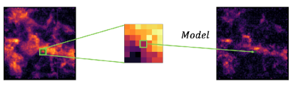
Figure 1: Graphical representation of the simplified modeling task demonstrating splitting a $\ce{CO}$ column density $\mathrm{1^{\circ}\times 1^{\circ}}$ region (left) into smaller patches (center) which are associated with their respective target values in the $\ce{{}^{13}CO}$ region (right).

The central idea of this paper is to harness machine learning (ML), in particular deep learning [14], to predict the distribution of $\ce{{}^{13}CO}$ based on the $\ce{CO}$ observation, and therefore infer the $\mathrm{H_{2}}$ small scale structure in regions where $\ce{{}^{13}CO}$ observations do not exist. Since a straightforward and robust analytical mapping between the two distributions is not available, ML could estimate this mapping from data. We train a deep learning model to map between $\ce{CO}$ and $\ce{{}^{13}CO}$ column densities in the Mopra region. To simplify this regression problem and enlarge our effective data set, we subdivide the maps into small $D_{1}\times D_{2}$ sections (patches) of the sky to their respective center points (Fig. 1). The validity of this simplification requires the gas column density to be locally correlated. That is, we assume it is unlikely that pixels outside of our chosen patch will significantly change the $\ce{{}^{13}CO}$ estimate. This simplification greatly reduces the model size and provides us with an effective data set of over $50$ million patches when $D_{1}=D_{2}=0.0581\degree$, or 7 pixels. We find that larger patch sizes do not improve model accuracy, justifying this assumption. We also apply smoothing techniques to eliminate noise from the data. The $\ce{CO}$$\rightarrow$$\ce{{}^{13}CO}$ modeling problem may now be formally written as finding a parameterized function $f_{\theta}$ mapping a source region $S\in\mathbb{R}^{D_{1}\times D_{2}}$ to an estimate target column density at the center of that same region $T\in\mathbb{R}$. The source $S_{i}$ corresponds to Mopra $\ce{CO}$ column densities and the targets $T_{i}$ to the corresponding $\ce{{}^{13}CO}$ column densities at the center of the patch (Fig. 1). We evaluate our estimates by splitting the Mopra region into independent sub-regions which we designate for training and testing. We employ different splitting choices, but we report on one, the Alternate Tiled split, throughout the remainder of this paper. This split consists of alternating $1^{\circ}\times 1^{\circ}$ regions (or tiles), training on tiles containing longitudes $\{301-302,\dots,349-350\}$ and testing on tiles containing $\{300-301,\dots,348-349\}$. This allows us to evaluate the model’s performance for neighbouring regions, reducing the variance between training and testing data distributions.

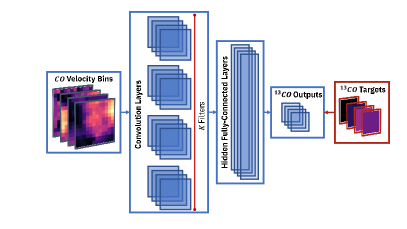
Figure 2: A diagram of the internal layers of the network. For simplicity, only 4 velocity bins are shown, whereas the full network uses all 17 velocity bins. The fully connected layers share weights and the same layers are applied to every velocity bin.

Figure 3: Top: the Modified Excess Template (from [1]). Bottom: the Smart Excess Template. The color scale (logarithmic) indicates the $\gamma$-ray intensity per 0.03125² degree pixel. The first tile to the left (closest to the GC, and covering longitudes ${349-350}$) is testing data, and the neighboring one is training data for the CNN. The interleaving pattern of testing and training tiles is adopted for the entire Mopra region.

We employ convolutional neural networks (CNNs) to model and predict the $\ce{{}^{13}CO}$ column density in a translation-invariant manner. CNNs use neurons with shared connection parameters in order to implement convolution operations that provide the basis for building translation invariant architectures [14]. Each convolution operation is associated with a kernel, or filter, corresponding to a set of connection weights that are shared by all the neurons in the corresponding layer. For each of the $17$ velocity bins, we apply $K$ learnable convolution filters of size $D_{1}\times D_{2}$, operating on an entire patch and independently for each velocity bin, producing $17$ $K$-dimensional latent vectors for each patch. Afterwards, we apply parametric rectified linear units ($PReLU$) [15, 16, 17] with a learnable slope, a batch normalization layer [18], and a random dropout layer [19, 20]. The latent vectors are then processed by several fully-connected layers, each with their own $PReLU$, batch-normalization, and dropout. Unlike the convolution layer, these hidden layers are shared between velocity bins, learning identical weights for every bin. This design allows spatial components (CNN) of the network to be specialized for each velocity bin while allowing latent higher level components to be shared between bins. The resulting latent vectors are fed through a final fully-connected layer which produces the $\ce{{}^{13}CO}$ concentration point estimates for each patch and velocity bin. A diagram of the network architecture is presented in Figure 2.

Figure 4: The pixel-wise residuals for the full region between the predicted counts from the Smart Excess Template and the predicted counts from the Modified Excess Template. Top: residual in counts (Smart-Modified), Middle: fractional residuals ((Smart-Modified)/Modified), Bottom: Residual in units of 1 standard deviation for the Modified Excess Template ((Smart-Modified)/$\sqrt{\mathrm{Modified}}$). The color scale is per 0.08² degree pixel.

The Mopra dataset contains varying regions of column densities from bright to very dim. To effectively learn this high-spread distribution, we model the incidence of photons on the Mopra detector as a Poisson process and use a Poisson log-likelihood loss. We further re-weight this loss based on the $\ce{{}^{13}CO}$ density to elevate the importance of bright pixels, prioritizing accuracy in hot-spots over a slight degradation in the background. This increases the importance of accurate measurement in the bright regions, encouraging the network to focus on the accuracy of these regions first. As the network trains, we anneal this weighting back to uniform (with all target values having equal weighting) in order to minimize any bias introduced by this loss. The design of this loss is guided by the overall goal of finding small angular scale features while limiting the amount of overestimation throughout the Mopra region.

We tune the CNN’s hyperparameters using the SHERPA hyperparameter optimization library [21, 22], testing 2000 network variations, scoring each parameterization with Poisson likelihood, and using Gaussian Process optimization to suggest parameters. Our final parameterization is evaluated after training the network for $200$ iterations. We generate the predicted $\ce{{}^{13}CO}$ density by stitching the network output for every patch in a source image. When performed on a single Nvidia Titan XP GPU, and batching $8192$ patches at once, this inference process requires approximately $11$ seconds to cover the entire Mopra region.

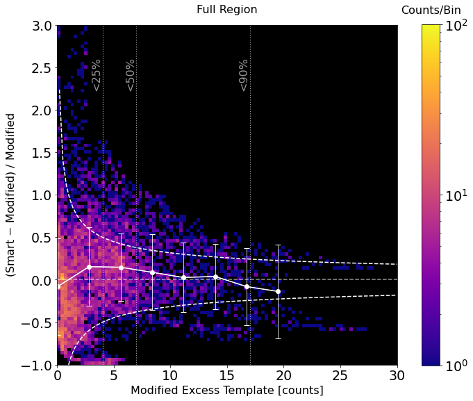
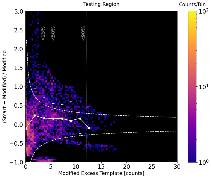
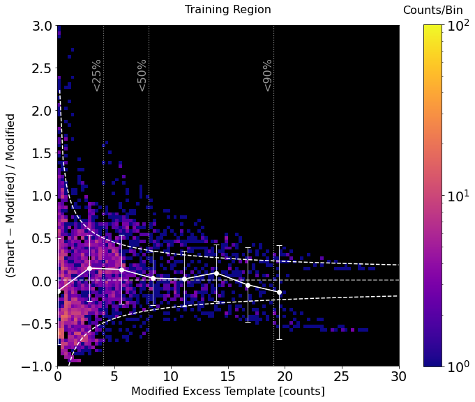
Figure 5: The fractional residuals between the nominal Smart Excess Template (Smart) and Modified Excess Template (Modified) predicted counts per pixel as a function of Modified Excess Template pixel counts for all tiles (left), testing tiles (center), and training tiles (right). The points and error bars represent the median and median absolute deviation of the fractional difference for the pixels in 8 domain intervals (we note that the scatter of the points within each interval is not simply characterized by these quantities and does not always indicate a most probable outcome.) We also plot the boundaries of the $\pm 1\sigma$ of the Poisson noise fluctuations of the Modified Excess Template. We overlay the 25%, 50%, 95% flux percentiles to indicate the flux fraction encompassed by pixels below that threshold.

Following the same procedure as in [1], we employ the CR propagation code GALPROP (v56)[23, 24, 25, 26, 27, 28, 29, 30, 31, 32, 33] to calculate $\gamma$-ray sky maps in 17 Galactocentric radial bins for the $\mathrm{H_{2}}$-related emission, where the latter is traced by $\ce{CO}$ and $\ce{{}^{13}CO}$. The $\ce{CO}$  and $\ce{{}^{13}CO}$  related $\mathrm{H_{2}}$ column densities, $N(\mathrm{H_{2}})_{\mathrm{CO13}}$ and $N(\mathrm{H_{2}})_{\mathrm{CO}}$ respectively, are used to determine the $\mathrm{H_{2}}$ that is missed in dense regions when only CO is used as a tracer. We follow the procedure from [1] to determine the Modified Map and “Modified Excess Template” (Fig. 3, top panel) to construct their ML analogs. The “Smart Map” is determined similarly to the Modified Map, but instead of using the true Mopra $\ce{{}^{13}CO}$  data, we use the $\ce{{}^{13}CO}$  estimates from the CNN. We use this to determine the ”Smart Excess Template”, defined as the difference between the Smart map and the baseline $\ce{CO}$ map. The Smart Excess Template, also integrated over all annuli and energies, is shown in Fig. 3, bottom panel. The map covers the full Mopra region, which includes alternating training and testing tiles for the CNN.

To assess how closely the CNN predicts the $\gamma$-ray  emission inferred by Mopra observations, we compare the excess templates with three different metrics. We quantify the differences with the following three metrics which are determined by using the predicted photon counts per pixel for each of the templates and scaled to $\sim$12 years of Fermi–LAT data (we assume the same Fermi–LAT observation parameters and event selection as for the simulations described in  [1] and in this work): absolute difference (Smart-Modified), fractional difference ((Smart-Modified)/Modified), difference in units of the standard deviation, $\sigma$, for the Modified counts ((Smart-Modified)/$\sqrt{{\mathrm{Modified}}}$). The latter metric allows us to compare the magnitude of the differences due to the CNN performance in light of the statistical power of the data. All results are shown in Fig. 4 as a function of longitude and latitude for the Mopra region. We observe that for the vast majority of the region (83.6% of the pixels), the predicted counts for the Smart Excess Template are within $\pm 1\sigma$ of the Modified Excess Template counts, and therefore the difference is generally within the statistical uncertainty of the data. This result indicates that the CNN performance is adequate for modeling the small scale structure in $\mathrm{H_{2}}$-related $\gamma$-ray emission traced by Mopra, for the statistics achieved by Fermi–LAT.

The CNN performance varies with respect to longitude. Most tiles display either an overall underprediction by the CNN across the entire tile or an overprediction, rather than a comparable mixture of under/over predictions across the same tile. This may be explained by the design of the loss function, placing increased importance towards brighter pixels while also biasing the network to prefer underprediction via Poisson regression. Prominent examples include the training tile $343^{\circ}<l<344^{\circ}$ and testing tile $348^{\circ}<l<349^{\circ}$, the brightest in each dataset, where the CNN underpredicts the gas column density, as shown in Fig. 4. The dependence of the residuals as a function of pixel brightness (in counts/pixel), is shown in Fig. 5 for the full Mopra region, and for the training and testing regions separately. Generally, better agreement between Mopra (Modified Excess Template) and the CNN prediction (Smart Excess Template) is found for the brighter pixels. There is a broad spread in the fractional residuals, but it is confined to be between $\pm$50% for the vast majority of the pixels. We overlay contours to indicate the $\pm$1$\sigma$ statistical fluctuations in the Modified Excess Template, which encompasses 83.6% of the pixels. We also overlay the median and median absolute deviation of the fractional difference in bins of the Modified Excess Template counts to guide the eye, but emphasize that the scatter of the points within each interval cannot be simply characterized by these quantities and does not always indicate a most probable outcome. As expected, we find that the CNN performs (somewhat) better in the training tiles. Approximately 58% of pixels where the CNN prediction is beyond the $\pm 1\sigma$ level are in the testing regions. The CNN is more likely to overpredict the emission for the dimmer pixels (60.8% of pixels across the full region are below the 25% flux percentile), consistently with the design. The CNN overprediction in the dim pixels essentially spreads out the brightness of hot-spots over a larger area. We also note that small statistics causes the fractional difference to increase dramatically for the faintest pixels. Above the 90% flux percentile, the distribution of the fractional residuals bifurcates into two separate distribution. The underpredicted pixels are in the $343^{\circ}<l<344^{\circ}$ tile, and the overpredicted pixels are in $333^{\circ}<l<334^{\circ}$ tile, both in the training regions. This is likely caused by our choice to combine independent convolution layers for each velocity bin with a shared hidden layer. Since certain bins have higher overall brightness than others, the shared hidden layer will attempt to average the error between the two extremes.

We determine the significance of the Smart Excess Template in the Fermi–LAT data, similarly to [1] for the Modified Excess Template. The simulations cover the same observations and event selection ($\sim$12 years, $1-100$ GeV, P8R3 CLEAN FRONT+BACK). We only simulate the $\mathrm{H_{2}}$-related $\gamma$-ray emission in the Mopra region, excluding all other components, since our goal is to establish the performance of the Smart Excess Template in the optimistic scenario where all other components are known. The simulated events trace the $\mathrm{H_{2}}$-related $\gamma$-ray emission modeled with the Modified Map from Mopra. The simulated data are fit based on a binned maximum likelihood method to a model that includes the baseline $\ce{CO}$ map (as observed by Mopra) and the Smart Excess Template. The normalization of the Smart Excess Template is free to vary in the fit. The energy spectrum, calculated by GALPROP, is assumed, and held fixed during the likelihood fit. The normalization and spectral index of the $\ce{CO}$ baseline contribution is also free to vary. The 17 radial bins from GALPROP are combined into 4 radial annuli, which we refer to as A1, A2, A3, and A4, with the same partitioning as in [1]. Also consistently to [1], the normalization of A4 is held constant to a normalization of 1.0, contributing a partial flux of $4.98\times 10^{-9}$ $\mathrm{p}\mathrm{h}\,\mathrm{c}\mathrm{m}^{-2}\,\mathrm{s}^{-1}$.

We simulate 1000 realizations and calculate the Test Statistics (TS) for the nested models ($\mathrm{-2log(L_{0}/L)}$, where $\mathrm{L_{0}}$ is the null hypothesis (CO baseline), and $\mathrm{L}$ is the alternative hypothesis (CO baseline and Smart Excess Template.) The statistical significance is approximated by $\sigma\approx\sqrt{\mathrm{TS}}$.

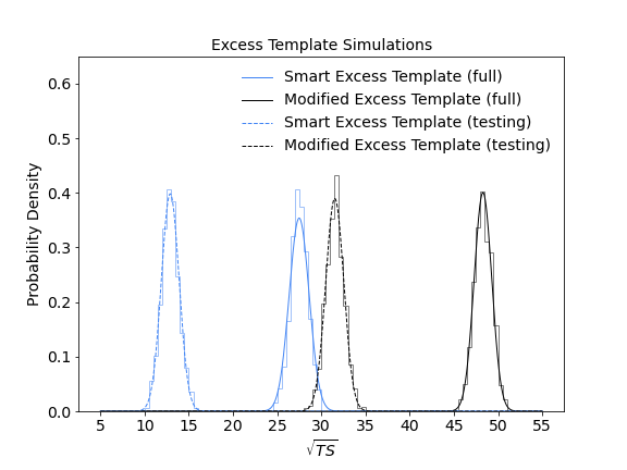
Figure 6: Statistical significance of the Smart Excess Template for the full Mopra region (solid lines), and for the testing regions (dashed lines). Each contains 1000 realizations of 12 years of Fermi–LAT data. A fit with a Gaussian distribution is overlaid to each distribution. These distributions are compared to the results for the Modified Excess Template from [1].

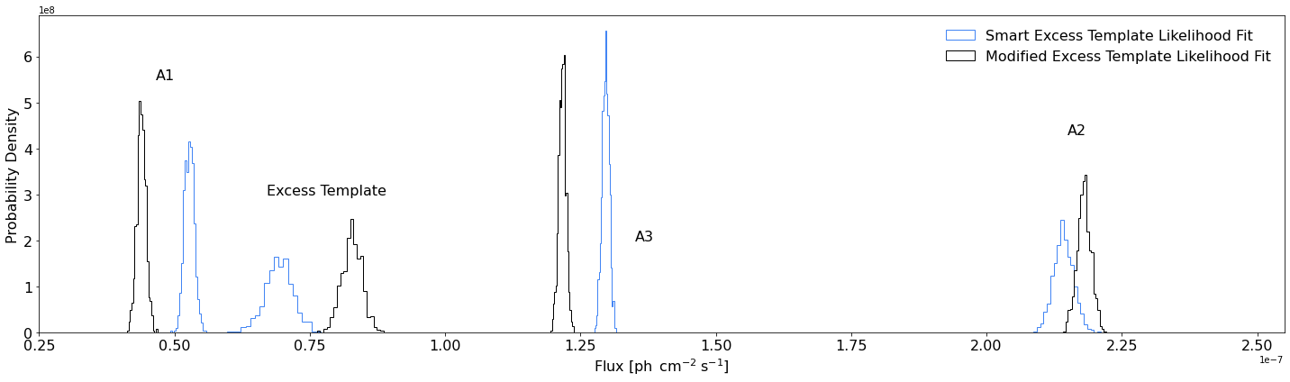
Figure 7: Distribution of fluxes for each component of the best-fit model using the Smart Excess Template maps over the full region for 1000 simulations of Fermi–LAT data. The results for the Modified Excess Template maps from [1] are overlaid. Note that one of the annuli (A4), not shown, has negligible contribution and the normalization was fixed in the fitting process.

The distribution of the $\sqrt{TS}$ for the simulations is shown in Fig. 6 for the full Mopra region (solid line), and for the testing regions only (dashed line). The Smart Excess Template corresponds to $\sqrt{TS}=27.5\pm 1.1$ (mean and standard deviation) in the full Mopra region and $12.9\pm 1.0$ in the testing region. The significance in the testing region is lower, not only because of the smaller statistics, but also because the full region contains the training tiles where the CNN more closely matches the Mopra data. For comparison, the Modified Excess Template has a $\sqrt{TS}=48.3\pm 1.0$ and $\sqrt{TS}=31.5\pm 1.0$ for the full and testing regions, respectively.

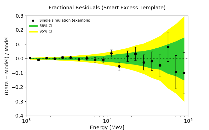
Figure 8: Fractional count residuals for the fit with the Smart Excess Template. The green and yellow bands show the 68% and 95% confidence regions from 1000 simulations, respectively. We also plot the results for a single simulation as an example in each case, which is shown with black data points.

Figure 9: Fractional count residuals, (Data-Model)/Model, in latitude and longitude for the fits with the Smart Excess Template, in addition to the other $\ce{CO}$ components. The residuals are calculated using the mean over 1000 simulations.

In Fig. 7, we show the distributions for the best-fit flux of the Smart Excess Template overlaid with those for the Modified Excess Template, as well as the flux for the CO baseline emission, separated into annuli. The integrated flux for the Smart Excess Template is approximately 83.7% of the flux of the Modified Excess Template, indicating an overall underprediction by the CNN. The fractional count residuals ((Data-Model)/Model) as a function of energy for the best fit model are shown in Fig. 8 for the fits that include Smart Excess Template, in addition to the other $\ce{CO}$ components. They are consistent with zero. The best fit spectra of the $\ce{CO}$ components agree with the GALPROP prediction. Finally, Fig. 9 shows the fractional count residuals in latitude, longitude. The residuals, which incorporate differences between the (best fit) Smart Excess Template and the (simulated) Modified Excess Template, are smaller than those shown in Fig. 4, (middle panel) indicating the other CO model components partially compensate for the discrepancies between the Excess Templates. We have performed this analysis also using Gaussian Processes and find that the performance is worse compared to the CNN.

The ML methodology presented here must be refined to be extended to other regions of the sky. The available all sky $\ce{CO}$ $J$=1–0 observations have significantly poorer spatial resolution (8^′ from [34]) compared to Mopra ($0.6^{\prime}$). The CNN model will therefore require additional transfer learning to operate on lower resolution maps. The resolution of the Fermi–LAT data is worse (for most energies and event types), suggesting that the impact of the poorer $\ce{CO}$ resolution on the CNN predictions for the $\gamma$-rays might ultimately be less pronounced. Another consideration is that the available $\ce{{}^{13}CO}$ training data for the CNN (from Mopra, and other observations [35, 36, 37, 38, 39] that could also be included), are confined to the Galactic plane. The $\mathrm{H_{2}}$ scale height is low, but its small scale structure contribution at higher latitudes might not be negligible because of the contribution of more local $\mathrm{H_{2}}$. However, because of the lack of adequate training data the CNN prediction for this component could be more uncertain and this is relevant for the characterization of the GC excess, which extends to high latitudes. Finally, this analysis inherits the limitations and uncertainties in modeling the $\mathrm{H_{2}}$ component with traditional methods, including the loss of kinematic resolution for the gas in the direction of the GC [40]. And it adds another: the $\mathrm{H_{2}}$ column densities from $\ce{CO}$ and $\ce{{}^{13}CO}$ have been treated independently in this work. Their estimates can be related analytically, but rely on a assumptions pertaining to the optical depth, beam filling factor, spatial variation, etc. (e.g. [41, 42]). More ambitiously, ML may be used to constrain some of these uncertainties by using the $\gamma$-ray data. Finally, small scale structure in the $\gamma$-ray data could also arise from other components of the IE, e.g. related to $\ce{H\textsc{i}}$, and shall be included in a more comprehensive study.

Conclusions.— We present a methodology that harnesses ML to predict the small scale component of the interstellar $\mathrm{H_{2}}$ gas and its related $\gamma$-ray emission for the first time. Incorporating this contribution in $\gamma$-ray IE models is crucial as it impacts the determination of $\gamma$-ray point sources and could affect characterization of extended $\gamma$-ray emissions, e.g. the Fermi–LAT GC excess. To this end, we employ observations of tracers of this emission, which are only available in limited regions of the sky (covered by the Mopra survey), and train a CNN to predict this component elsewhere. We have tested the performance of this methodology in predicting the contribution of the $\mathrm{H_{2}}$ related small scale structure to the Fermi–LAT data and conclude that deep learning can model the $\gamma$-ray emission well in data-rich regions supporting prospects to employ and extend this methodology to other regions of the sky.

I Acknowledgements

We thank Troy Porter for many helpful discussions and insights. The work of AS, MT, and PB is in part supported by grants NSF NRT 1633631 and ARO 76649-CS to PB.

References

- Karwin et al. [2022] C. Karwin, A. Broughton, S. Murgia, A. Shmakov, M. Tavakoli, and P. Baldi, Improved modeling of the discrete component of the galactic interstellar -ray emission and implications for the Fermi–lat galactic center excess (2022).
- Ballet et al. [2020] J. Ballet, T. H. Burnett, S. W. Digel, and B. Lott, Fermi Large Area Telescope Fourth Source Catalog Data Release 2, arXiv e-prints , arXiv:2005.11208 (2020), arXiv:2005.11208 .
- Goodenough and Hooper [2009] L. Goodenough and D. Hooper, Possible evidence for dark matter annihilation in the inner milky way from the fermi gamma ray space telescope (2009), arXiv:0910.2998 [hep-ph] .
- Hooper and Goodenough [2011] D. Hooper and L. Goodenough, Dark Matter Annihilation in The Galactic Center As Seen by the Fermi Gamma Ray Space Telescope, Phys. Lett. B 697, 412 (2011), arXiv:1010.2752 [hep-ph] .
- Hooper and Linden [2011] D. Hooper and T. Linden, Origin of the gamma rays from the galactic center, Phys. Rev. D 84, 123005 (2011).
- Abazajian [2011] K. N. Abazajian, The consistency of fermi-LAT observations of the galactic center with a millisecond pulsar population in the central stellar cluster, Journal of Cosmology and Astroparticle Physics 2011 (03), 010.
- Abazajian et al. [2014] K. Abazajian, N. Canac, S. Horiuchi, and M. Kaplinghat, Astrophysical and dark matter interpretations of extended gamma ray emission from the galactic center, Physical Review D 90 (2014).
- Gordon and Macías [2013] C. Gordon and O. Macías, Dark matter and pulsar model constraints from galactic center fermi-lat gamma-ray observations, Phys. Rev. D 88, 083521 (2013).
- Daylan et al. [2016] T. Daylan, D. P. Finkbeiner, D. Hooper, T. Linden, S. K. Portillo, N. L. Rodd, and T. R. Slatyer, The characterization of the gamma-ray signal from the central milky way: A case for annihilating dark matter, Physics of the Dark Universe 12, 1 (2016).
- Calore et al. [2015] F. Calore, I. Cholis, and C. Weniger, Background model systematics for the fermi GeV excess, Journal of Cosmology and Astroparticle Physics 2015 (03), 038.
- Ajello et al. [2016] M. Ajello, A. Albert, W. Atwood, G. Barbiellini, D. Bastieri, K. Bechtol, R. Bellazzini, E. Bissaldi, R. Blandford, E. Bloom, et al., Fermi-lat observations of high-energy -ray emission toward the galactic center, The Astrophysical Journal 819, 44 (2016).
- Murgia [2020] S. Murgia, The Fermi–LAT Galactic Center Excess: Evidence of Annihilating Dark Matter?, Ann. Rev. Nucl. Part. Sci. 70, 455 (2020).
- Braiding et al. [2018] C. Braiding, G. F. Wong, N. I. Maxted, D. Romano, M. G. Burton, R. Blackwell, M. D. Filipović, M. S. R. Freeman, B. Indermuehle, J. Lau, and et al., The mopra southern galactic plane co survey—data release 3, Publications of the Astronomical Society of Australia 35, 10.1017/pasa.2018.18 (2018).
- Baldi [2021] P. Baldi, Deep Learning in Science: Theory, Algorithms, and Applications (Cambridge University Press, Cambridge, UK, 2021) in press.
- Agostinelli et al. [2014] F. Agostinelli, M. Hoffman, P. Sadowski, and P. Baldi, Learning activation functions to improve deep neural networks, arXiv preprint arXiv:1412.6830 (2014).
- He et al. [2015] K. He, X. Zhang, S. Ren, and J. Sun, Delving deep into rectifiers: Surpassing human-level performance on imagenet classification, CoRR abs/1502.01852 (2015), 1502.01852 .
- Tavakoli et al. [2021] M. Tavakoli, F. Agostinelli, and P. Baldi, Splash: Learnable activation functions for improving accuracy and adversarial robustness, Neural Networks 140, 1 (2021).
- Ioffe and Szegedy [2015] S. Ioffe and C. Szegedy, Batch normalization: Accelerating deep network training by reducing internal covariate shift, in Proceedings of the 32nd International Conference on International Conference on Machine Learning - Volume 37, ICML’15 (JMLR.org, 2015) p. 448–456.
- Srivastava et al. [2014] N. Srivastava, G. E. Hinton, A. Krizhevsky, I. Sutskever, and R. Salakhutdinov, Dropout: a simple way to prevent neural networks from overfitting., Journal of Machine Learning Research 15, 1929 (2014).
- Baldi and Sadowski [2014] P. Baldi and P. Sadowski, The dropout learning algorithm, Artificial Intelligence 210C, 78 (2014).
- Hertel et al. [2018] L. Hertel, J. Collado, P. Sadowski, and P. Baldi, Sherpa: Hyperparameter optimization for machine learning models (openreview.net, 2018).
- Hertel et al. [2020] L. Hertel, J. Collado, P. Sadowski, J. Ott, and P. Baldi, Sherpa: Robust hyperparameter optimization for machine learning, SoftwareX (2020), in press.
- Moskalenko and Strong [1998] I. V. Moskalenko and A. W. Strong, Production and propagation of cosmic ray positrons and electrons, Astrophys. J. 493, 694 (1998), arXiv:astro-ph/9710124 [astro-ph] .
- Moskalenko and Strong [2000] I. V. Moskalenko and A. W. Strong, Anisotropic inverse Compton scattering in the galaxy, Astrophys. J. 528, 357 (2000), arXiv:astro-ph/9811284 [astro-ph] .
- Strong and Moskalenko [1998] A. W. Strong and I. V. Moskalenko, Propagation of cosmic-ray nucleons in the galaxy, Astrophys. J. 509, 212 (1998), arXiv:astro-ph/9807150 [astro-ph] .
- Strong et al. [2000] A. W. Strong, I. V. Moskalenko, and O. Reimer, Diffuse continuum gamma-rays from the galaxy, Astrophys. J. 537, 763 (2000), [Erratum: ApJ 541,1109(2000)], arXiv:astro-ph/9811296 [astro-ph] .
- Ptuskin et al. [2006] V. S. Ptuskin, I. V. Moskalenko, F. C. Jones, A. W. Strong, and V. N. Zirakashvili, Dissipation of Magnetohydrodynamic Waves on Energetic Particles: Impact on Interstellar Turbulence and Cosmic-Ray Transport, Astrophys. J. 642, 902 (2006), astro-ph/0510335 .
- Strong et al. [2007] A. W. Strong, I. V. Moskalenko, and V. S. Ptuskin, Cosmic-ray propagation and interactions in the Galaxy, ARNPS 57, 285 (2007), arXiv:astro-ph/0701517 [astro-ph] .
- Vladimirov et al. [2011] A. E. Vladimirov, S. W. Digel, G. Johannesson, P. F. Michelson, I. V. Moskalenko, P. L. Nolan, E. Orlando, T. A. Porter, and A. W. Strong, GALPROP WebRun: an internet-based service for calculating galactic cosmic ray propagation and associated photon emissions, Comput. Phys. Commun. 182, 1156 (2011), arXiv:1008.3642 [astro-ph.HE] .
- Jóhannesson et al. [2016] G. Jóhannesson et al., Bayesian analysis of cosmic-ray propagation: evidence against homogeneous diffusion, Astrophys. J. 824, 16 (2016), arXiv:1602.02243 [astro-ph.HE] .
- Porter et al. [2017] T. A. Porter, G. Johannesson, and I. V. Moskalenko, High-energy gamma rays from the milky way: Three-dimensional spatial models for the cosmic-ray and radiation field densities in the interstellar medium, Astrophys. J. 846, 23pp (2017).
- Johannesson et al. [2018] G. Johannesson, T. A. Porter, and I. V. Moskalenko, The Three-Dimensional Spatial Distribution of Interstellar Gas in the Milky Way: Implications for Cosmic Rays and High-Energy Gamma-Ray Emissions, Astrophys. J. 856, 45 (2018), arXiv:1802.08646 [astro-ph.HE] .
- Génolini et al. [2018] Y. Génolini, D. Maurin, I. V. Moskalenko, and M. Unger, Current status and desired precision of the isotopic production cross sections relevant to astrophysics of cosmic rays: Li, be, b, c, and n, PhRvC 98, 034611 (2018).
- Dame et al. [2001] T. M. Dame, D. Hartmann, and P. Thaddeus, The Milky Way in Molecular Clouds: A New Complete CO Survey, Astrophys. J. 547, 792 (2001), arXiv:astro-ph/0009217 [astro-ph] .
- Urquhart et al. [2018] J. S. Urquhart, C. König, A. Giannetti, S. Leurini, T. J. T. Moore, D. J. Eden, T. Pillai, M. A. Thompson, C. Braiding, M. G. Burton, T. Csengeri, J. T. Dempsey, C. Figura, D. Froebrich, K. M. Menten, F. Schuller, M. D. Smith, and F. Wyrowski, ATLASGAL - properties of a complete sample of Galactic clumps, Monthly Notices of the Royal Astronomical Society 473, 1059 (2018), arXiv:1709.00392 [astro-ph.GA] .
- Eden et al [2020] D. J. Eden et al, CHIMPS2: survey description and 12CO emission in the Galactic Centre, Monthly Notices of the Royal Astronomical Society 498, 5936 (2020), arXiv:2009.05073 [astro-ph.GA] .
- Kalberla et al. [2020] P. M. W. Kalberla, J. Kerp, and U. Haud, H I filaments are cold and associated with dark molecular gas. HI4PI-based estimates of the local diffuse CO-dark H2 distribution, Astronomy & Astrophysics 639, A26 (2020), arXiv:2004.14630 [astro-ph.GA] .
- Blackwell et al. [2017] R. Blackwell, M. Burton, and G. Rowell, Mopra Central Molecular Zone Carbon Monoxide Survey Status, in The Multi-Messenger Astrophysics of the Galactic Centre, Vol. 322, edited by R. M. Crocker, S. N. Longmore, and G. V. Bicknell (2017) pp. 164–165.
- Di Teodoro et al. [2018] E. M. Di Teodoro, N. M. McClure-Griffiths, F. J. Lockman, S. R. Denbo, R. Endsley, H. A. Ford, and K. Harrington, Blowing in the Milky Way Wind: Neutral Hydrogen Clouds Tracing the Galactic Nuclear Outflow, Astrophys. J. 855, 33 (2018), arXiv:1802.02152 [astro-ph.GA] .
- Ackermann et al. [2012] M. Ackermann, M. Ajello, W. Atwood, L. Baldini, J. Ballet, G. Barbiellini, D. Bastieri, K. Bechtol, R. Bellazzini, B. Berenji, et al., Fermi-lat observations of the diffuse -ray emission: implications for cosmic rays and the interstellar medium, The Astrophysical Journal 750, 3 (2012).
- Burton et al. [2013] M. G. Burton, C. Braiding, C. Glueck, P. Goldsmith, J. Hawkes, D. J. Hollenbach, C. Kulesa, C. L. Martin, J. L. Pineda, G. Rowell, et al., The mopra southern galactic plane co survey, Publications of the Astronomical Society of Australia 30 (2013).
- Cormier et al. [2018] D. Cormier, F. Bigiel, M. J. Jiménez-Donaire, A. K. Leroy, M. Gallagher, A. Usero, K. Sandstrom, A. Bolatto, A. Hughes, C. Kramer, M. R. Krumholz, D. S. Meier, E. J. Murphy, J. Pety, E. Rosolowsky, E. Schinnerer, A. Schruba, K. Sliwa, and F. Walter, Full-disc 13CO(1–0) mapping across nearby galaxies of the EMPIRE survey and the CO-to-H2 conversion factor, Monthly Notices of the Royal Astronomical Society 475, 3909 (2018), https://academic.oup.com/mnras/article-pdf/475/3/3909/23965800/sty059.pdf .