Policy Optimization for Markov Games: Unified Framework and Faster Convergence

Abstract

This paper studies policy optimization algorithms for multi-agent reinforcement learning. We begin by proposing an algorithm framework for two-player zero-sum Markov Games in the full-information setting, where each iteration consists of a policy update step at each state using a certain matrix game algorithm, and a value update step with a certain learning rate. This framework unifies many existing and new policy optimization algorithms. We show that the state-wise average policy of this algorithm converges to an approximate Nash equilibrium (NE) of the game, as long as the matrix game algorithms achieve low weighted regret at each state, with respect to weights determined by the speed of the value updates. Next, we show that this framework instantiated with the Optimistic Follow-The-Regularized-Leader (OFTRL) algorithm at each state (and smooth value updates) can find an $\mathcal{\widetilde{O}}(T^{-5/6})$ approximate NE in $T$ iterations, and a similar algorithm with slightly modified value update rule achieves a faster $\mathcal{\widetilde{O}}(T^{-1})$ convergence rate. These improve over the current best $\mathcal{\widetilde{O}}(T^{-1/2})$ rate of symmetric policy optimization type algorithms. We also extend this algorithm to multi-player general-sum Markov Games and show an $\mathcal{\widetilde{O}}(T^{-3/4})$ convergence rate to Coarse Correlated Equilibria (CCE). Finally, we provide a numerical example to verify our theory and investigate the importance of smooth value updates, and find that using “eage” value updates instead (equivalent to the independent natural policy gradient algorithm) may significantly slow down the convergence, even on a simple game with $H=2$ layers.

1 Introduction

Policy optimization, i.e. algorithms that learn to make sequential decisions by local search on the agent’s policy directly, is a widely used class of algorithms in reinforcement learning [38, 42, 43]. Policy optimization algorithms are particularly advantageous in the multi-agent reinforcement learning (MARL) setting (e.g. compared with value-based counterparts), due to their typically lower representational cost and better scalability in both training and execution. A variety of policy optimization algorithms such as Independent PPO [13], MAPPO [54], QMix [40] have been proposed to solve real-world MARL problems [4, 37, 41]. These algorithms share a same high-level structure with iterative value updates (for certain value estimates) and policy updates (often independently with each agent) using information from the value estimates and/or true rewards.

While policy optimization for MARL has been studied theoretically in a growing body of work, there are still gaps between algorithms used in practice and provably-efficient algorithms studied in theory—Algorithms in practice generally follow two natural design principles: symmetric updates among all agents, and simultaneous learning of values and policies [57, 54]. By contrast, policy optimization algorithms studied in theory often diverge from these principles and incorporate some tweaks, such as (i) asymmetric updates, where one agent takes a much smaller learning rate than the others (two time-scale) [11] or waits until the other agents learn an approximate best response [60]; and (ii) batch-like learning, where policies are optimized to sufficient precision with respect to the current value estimate before the next value update [8]. There is so far a lacking of systematic studies on the performance of the more vanilla policy optimization algorithms following the above two principles, even under the setting where full-information feedback from the game is available.

Towards bridging these gaps, this paper studies policy optimization algorithms for Markov games, with a focus on algorithms with symmetric updates and simultaneous learning of values and policies. Our contributions can be summarized as follows:

• We propose an algorithm framework for two-player zero-sum Markov games in the full-information setting (Section 3). This framework unifies many existing and new policy optimization algorithms such as Nash V-Learning, Gradient Descent/Ascent, as well as seemingly disparate algorithms such as Nash Q-Learning (Section 3.2). We prove that the state-wise average policy outputted by the above algorithm is an approximate Nash Equilibrium (NE), so long as suitable per-state weighted regrets are bounded (Section 3.1). This generic result can be instantiated in a modular fashion to derive convergence guarantees for the many examples above.

• We instantiate our framework to show that a new algorithm based on Optimistic Follow-The-Regularized-Leader (OFTRL) and smooth value updates finds an $\widetilde{\mathcal{O}}(T^{-5/6})$ approximate NE in $T$ iterations (Section 4). This improves over the current best rate of $\widetilde{\mathcal{O}}(T^{-1/2})$ achieved by symmetric policy optimization type algorithms. In addition, we also propose a slightly modified OFTRL algorithm that further improves the rate to $\widetilde{\mathcal{O}}(T^{-1})$, which matches with the known best rate for all policy optimization type algorithm.

• We additionally extend the above OFTRL algorithm to multi-player general-sum Markov games and show an $\widetilde{\mathcal{O}}(T^{-3/4})$ convergence rate to Coarse Correlated Equilibria (CCE), which is also the first rate faster than $\widetilde{\mathcal{O}}(T^{-1/2})$ for policy optimization in general-sum Markov games (Section 4.1).

• We perform simulations on a carefully constructed zero-sum Markov game with $H=2$ layers to verify our convergence guarantees. The numerical tests further suggest the importance of smooth value updates: the Independent Natural Policy Gradient algorithm (as one instantiation of our algorithm framework with “eager” value updates) appears to converge much slower (Section 5).

1.1 Related work

Two-player zero-sum MGs

Markov games (MGs) [28] (also known as Stochastic Games [45]) is a widely studied model for multi-agent reinforcement learning. In the most basic setting of two-player zero-sum MGs, algorithms for computing the NE have been extensively studied in both the full-information setting [29, 19, 18] and the sample-based/online setting [6, 50, 21, 46, 56, 2, 53, 3, 31, 24, 20, 55, 10, 32]. Our algorithm framework incorporates (the full-information version of) several algorithms in this line of work.

Policy optimization for zero-sum MGs

Policy optimization for single-agent Markov Decision Processes has been extensively in a recent line of work, e.g. [1, 5, 30, 44, 35, 33, 7, 14, 52] and the many references therein. For two-player zero-sum MGs, the Nash V-Learning algorithm of Bai et al. [3] (originally proposed for the sample-based online setting) can be viewed as an independent policy optimization algorithm, and can be adapted to the full-information setting with $\widetilde{\mathcal{O}}(T^{-1/2})$ convergence rate. Daskalakis et al. [11] prove that the independent policy gradient algorithm with an asymmetric two time-scale learning rate can learn the NE (for one player only) with polynomial iteration/sample complexity. Zhao et al. [60] show that another asymmetric algorithm that simulates a policy gradient/best response dynamics converges to NE with $\widetilde{\mathcal{O}}(1/T)$ rate. Cen et al. [8] use a symmetric optimistic (extragradient) subroutine for matrix games to learn zero-sum MGs in a layer-wise fashion (more like a Value Iteration type algorithm), and also derive an $\widetilde{\mathcal{O}}(1/T)$ convergence rate. The closest to our work is Wei et al. [51] which proves that Optimistic Gradient Descent/Ascent (OGDA), combined with smooth value updates at all layers simultaneously, converges to an NE with $\widetilde{\mathcal{O}}(T^{-1/2})$ rate for both the average duality gap and the last iterate. The $\widetilde{\mathcal{O}}(T^{-5/6})$ rate of our OFTRL algorithm improves over [51] and is the first such faster rate for symmetric, policy optimization type algorithms. The $\widetilde{\mathcal{O}}(1/T)$ rate of our modified OFTRL algorithm matches with rates in [60, 7], while still maintaining symmetric update and simultaneous learning of values and policies.

Multi-player general-sum MGs

A recent line of work shows that a generalization of the V-learning algorithm to the multi-player general-sum setting can learn Coarse Correlated Equilibria (CCE) [47, 23, 34] and Correlated Equilibria (CE) [47, 23]. The algorithmic designs in these works are specially tailored to the sample-based setting, where the best possible rate is $\widetilde{\mathcal{O}}(T^{-1/2})$. In contrast, this paper considers the full-information setting and proposes new algorithms achieving the faster $\widetilde{\mathcal{O}}(T^{-3/4})$ for learning CCE in general-sum MGs. Another recent line of work considers learning NE in Markov Potential Games [58, 27, 47, 15, 59], which can be seen as a cooperative-type subclass of general-sum MGs.

Optimistic algorithms in normal-form games

Technically, our accelerated rates build on the recent line of work on faster rates for optimistic no-regret algorithms in normal-form games [48, 39, 9, 12]. Specifically, our $\tilde{\mathcal{O}}(T^{-5/6})$ rate for two-player zero-sum MGs builds upon a first-order smoothness analysis of [9], our improved $\widetilde{\mathcal{O}}(T^{-1})$ rate in the same setting (achieved by the modified OFTRL algorithm) leverages analysis of [39, 48] on bounding the summed regret over the two players, and our $\tilde{\mathcal{O}}(T^{-3/4})$ rate for multi-player general-sum MGs follows from the RVU-property [48, Definition 3]. Our incorporation of these techniques involves non-trivial new components such as weighted first-order smoothness bounds and handling changing game rewards.

2 Preliminaries

We consider the tabular episodic (finite-horizon) two-player-zero-sum Markov games (MGs), which can be denoted as $\mathcal{M}(H,\mathcal{S},\mathcal{A},\mathcal{B},\mathbb{P},r)$, where $H$ is the horizon length; $\mathcal{S}$ is the state space with $|\mathcal{S}|=S$; $\mathcal{A},\mathcal{B}$ are the action space of the max-player and min-player respectively, with $|\mathcal{A}|=A,|\mathcal{B}|=B$; $\mathbb{P}=\{\mathbb{P}_{h}\}_{h=1}^{H}$ is the transition probabilities, where each $\mathbb{P}_{h}(s^{\prime}|s,a,b)$ gives the probability of transition to state $s^{\prime}$ from state-action $(s,a,b)$; $r=\{r_{h}\}_{h=1}^{H}$ are the reward functions, such that $r_{h}(s,a,b)$ is reward of the max-player and $-r_{h}(s,a,b)$ is the reward of the min-player at time step $h$ and state-action $(s,a,b)$. In each episode, the MG starts with a deterministic initial state $s_{1}$. Then at each time step $1\leq h\leq H$, both players observes the state $s_{h}$, the max-player takes an action $a_{h}\in\mathcal{A}$, and the min-player takes an action $b_{h}\in\mathcal{B}$. Then, both players receive their rewards $r_{h}(s_{h},a_{h},b_{h})$ and $-r_{h}(s_{h},a_{h},b_{h})$, respectively, and the system transits to the next state $s_{t+1}\sim\mathbb{P}_{h}(\cdot|s_{h},a_{h},b_{h})$.

Policies & value functions

A (Markov) policy $\mu$ of the max-player is a collection of policies $\mu=\{\mu_{h}:\mathcal{S}\to\Delta_{\mathcal{A}}\}_{h=1}^{H}$, where each $\mu_{h}(\cdot|s_{h})\in\Delta_{\mathcal{A}}$ specifies the probability of taking action $a_{h}$ at $(h,s_{h})$. Similarly, a (Markov) policy $\nu$ of the min-player is defined as $\nu=\{\nu_{h}:\mathcal{S}\to\Delta_{\mathcal{B}}\}$. For any policy $(\mu,\nu)$ (not necessarily Markov), we use $V_{h}^{\mu,\nu}:\mathcal{S}\to\mathbb{R}$ and $Q_{h}^{\mu,\nu}:\mathcal{S}\times\mathcal{A}\times\mathcal{B}\to\mathbb{R}$ to denote the value function and Q-function at time step $h$, respectively, i.e.

$$\textstyle V_{h}^{\mu,\nu}(s) \textstyle:=\mathbb{E}_{\mu,\nu}{\left[\sum_{h=h^{\prime}}^{H}r_{h^{\prime}}(s_{h^{\prime}},a_{h^{\prime}},b_{h^{\prime}})~{}|~{}s_{h}=s\right]},$$ (1)

$$\textstyle Q_{h}^{\mu,\nu}(s,a,b) \textstyle:=\mathbb{E}_{\mu,\nu}{\left[\sum_{h=h^{\prime}}^{H}r_{h^{\prime}}(s_{h^{\prime}},a_{h^{\prime}},b_{h^{\prime}})~{}|~{}s_{h}=s,a_{h}=a,b_{h}=b\right]}.$$ (2)

For notational simplicity, we use the following abbreviation: $[\mathbb{P}_{h}V](s,a,b):=\mathbb{E}_{s^{\prime}\sim\mathbb{P}_{h}(\cdot|s,a,b)}V(s^{\prime})$ for any value function $V$. By definition of the value functions and Q-functions, we have the following Bellman equations

$$Q_{h}^{\mu,\nu}(s,a,b) ={\left(r_{h}+\mathbb{P}_{h}V_{h+1}^{\mu,\nu}\right)}(s,a,b),$$

$$V_{h}^{\mu,\nu}(s,a,b) =\mathbb{E}_{a\sim\mu_{h}(\cdot|s),b\sim\nu_{h}(\cdot|s)}{\left[Q_{h}^{\mu,\nu}(s,a,b)\right]}=\left\langle Q_{h}^{\mu,\nu}(s,\cdot,\cdot),\mu(\cdot|s)\times\nu(\cdot|s)\right\rangle.$$

The goal for the max-player is to maximize the value function, whereas the goal for the min-player is to minimize the value function.

Best response & Nash equilibrium

For any Markov policy $\mu$ of a max-player, there exists a best response for the min-player, which can be taken as a Markov policy $\nu^{\dagger}(\mu)$ such that $V_{h}^{\mu,\nu^{\dagger}(\mu)}(s)=\inf_{\nu}V_{h}^{\mu,\nu}(s)$ for all $(s,h)\in\mathcal{S}\times[H]$. For simplicity we define $V_{h}^{\mu,\dagger}:=V_{h}^{\mu,\nu^{\dagger}(\mu)}$. By symmetry, we can also define $\mu^{\dagger}(\nu)$ and $V_{h}^{\dagger,\nu}$. It is known (e.g. [16]) that there exist Markov policies $(\mu^{\star},\nu^{\star})$ that perform optimally against best responses. These policies are also equivalent to Nash Equilibria (NEs) of the game, where no player can gain by switching to a different policy unilaterally. It can also be shown that any NE $(\mu^{\star},\nu^{\star})$ satisfies the following minimax equation

$$\textstyle\sup_{\mu}\inf_{\nu}V_{h}^{\mu,\nu}(s)=V_{h}^{\mu^{\star},\nu^{\star}}(s)=\inf_{\nu}\sup_{\mu}V_{h}^{\mu,\nu}(s).$$

Thus, while the NE policy $(\mu^{\star},\nu^{\star})$ may not be unique, all of them share the same value functions, which we denote as $V_{h}^{\star}:=V_{h}^{\mu^{\star},\nu^{\star}}$. The Q-function $Q_{h}^{\star}$ can be defined similarly. In this paper, our main goal is to find an approximate NE, which is formally defined below.

Definition 1 ($\varepsilon$-approximate Nash Equilibrium).

For any $\varepsilon\geq 0$, a policy $(\mu,\nu)$ is an $\varepsilon$-approximate Nash Equilibrium ($\varepsilon$-NE) if ${\rm NEGap}(\mu,\nu)\mathrel{\mathop{:}}=V_{1}^{\dagger,\nu}(s_{1})-V_{1}^{\mu,\dagger}(s_{1})\leq\varepsilon.$

Additional notation

For any $(h,s)\in[H]\times\mathcal{S}$ and Q function $Q_{h}:\mathcal{S}\times\mathcal{A}\times\mathcal{B}\to\mathbb{R}$, we define shorthand $[(\mu_{h})^{\top}Q_{h}\nu_{h}](s)\mathrel{\mathop{:}}=\left\langle Q_{h}(s,\cdot,\cdot),\mu_{h}(\cdot|s)\times\nu_{h}(\cdot|s)\right\rangle$ for any policy $(\mu,\nu)$. Similarly, we let $[Q_{h}\nu_{h}](s,\cdot)\mathrel{\mathop{:}}=\mathbb{E}_{b\sim\nu_{h}(\cdot|s)}[Q_{h}(s,\cdot,b)]\in\mathbb{R}^{A}$, and $[Q_{h}^{\top}\mu_{h}](s,\cdot)\mathrel{\mathop{:}}=\mathbb{E}_{a\sim\mu_{h}(\cdot|s)}[Q_{h}(s,a,\cdot)]\in\mathbb{R}^{B}$. We use $A\vee B\mathrel{\mathop{:}}=\max\{A,B\}$.

3 An algorithm framework for zero-sum Markov games

We begin by presenting an algorithm framework that unifies many existing and new algorithms for two-player zero-sum Markov Games, and its performance guarantee that could be specialized to yield concrete convergence results for many specific algorithms.

Our algorithm framework, described in Algorithm 1, consists of two main components: the policy update step computing policies $(\mu^{t},\nu^{t})$, and the value update step computing the Q estimate $Q_{h}^{t}$’s.

Algorithm 1 Algorithm framework for two-player zero-sum Markov Games

1:  Require: Learning rate ${\left\{\beta_{t}\right\}}_{t\geq 1}\subset[0,1]$ (with $\beta_{1}=1$); Algorithm ${\sf MatrixGameAlg}$.

2:  Initialize: $Q_{h}^{0}(s,a,b)\leftarrow H-h+1$ for all $(h,s,a,b)\in[H]\times\mathcal{S}\times\mathcal{A}\times\mathcal{B}$.

3:  for $t=1,\dots,T$ do

4:     for $h=H,\dots,1$ do

5:        Policy update: Update policies for all $s\in\mathcal{S}$:

$$(\mu_{h}^{t}(\cdot|s),\nu_{h}^{t}(\cdot|s))\leftarrow{\sf MatrixGameAlg}{\left({\left\{Q_{h}^{i}(s,\cdot,\cdot)\right\}}_{i=1}^{t-1},{\left\{\mu_{h}^{i}(\cdot|s)\right\}}_{i=1}^{t-1},{\left\{\nu_{h}^{i}(\cdot|s)\right\}}_{i=1}^{t-1}\right)}.$$

6:        Value update: Update Q-value for all $(s,a,b)\in\mathcal{S}\times\mathcal{A}\times\mathcal{B}$:

$$Q_{h}^{t}(s,a,b)\leftarrow(1-\beta_{t})Q_{h}^{t-1}(s,a,b)+\beta_{t}{\left(r_{h}+\mathbb{P}_{h}[(\mu_{h+1}^{t})^{\top}Q_{h+1}^{t}\nu_{h+1}^{t}]\right)}(s,a,b).$$ (3)

7:  Output: State-wise average policy $(\widehat{\mu}^{T},\widehat{\nu}^{T})$, with $\beta_{T}^{t}$ defined in (6):

$$\textstyle\widehat{\mu}_{h}^{T}(\cdot|s)\leftarrow\sum_{t=1}^{T}\beta_{T}^{t}\mu_{h}^{t}(\cdot|s),\quad\widehat{\nu}_{h}^{T}(\cdot|s)\leftarrow\sum_{t=1}^{T}\beta_{T}^{t}\nu_{h}^{t}(\cdot|s)~{}~{}~{}\textrm{for all}~{}(h,s)\in[H]\times\mathcal{S}.$$ (4)

Policy update via matrix game algorithms

In the policy update step (Line 5), for each $(h,s)$, the two players update policies $(\mu^{t}_{h}(\cdot|s),\nu^{t}_{h}(\cdot|s))$ at $(h,s)$ using some matrix game algorithm ${\sf MatrixGameAlg}$ which takes as input all past Q matrices and all past policies of both players. The ${\sf MatrixGameAlg}$ offers a flexible interface that allows many choices such as the matrix NE subroutine over the most recent Q matrix ${\sf MatrixNE}(Q^{t-1}_{h}(s,\cdot,\cdot))$, or any independent no-regret algorithm (for both players), such as Follow-The-Regularized-Leader (FTRL) (10) or projected Gradient Descent-Ascent (11) considered in the examples later.

Value update with learning rate ${\left\{\beta_{t}\right\}}$

For any $(h,s,a,b)$, the value update step (Line 6) updates $Q_{h}^{t}(s,a,b)$ by the newest value function $r_{h}+\mathbb{P}_{h}[(\mu_{h+1}^{t})^{\top}Q_{h+1}^{t}\nu_{h+1}^{t}]$ propagated from layer $h+1$, using a sequence of learning rates ${\left\{\beta_{t}\right\}}_{t\geq 1}$ which we assume to be within $[0,1]$ (with $\beta_{1}\mathrel{\mathop{:}}=1$). ${\left\{\beta_{t}\right\}}$ controls the speed of the value update, with two important special cases:

1. Eager value updates, where we set $\beta_{t}=1$ so that $Q_{h}^{t}$ performs policy evaluation of the current policy $(\mu^{t},\nu^{t})$, that is, $Q_{h}^{t}=Q_{h}^{\mu^{t},\nu^{t}}$.

2. Smooth (incremental) value updates, where we choose $\beta_{t}\to 0$ as $t\to\infty$. In this case, the $Q_{h}^{t}$ moves slower (resembling a critic in Actor-Critic like algorithms), and becomes a weighted average of all past updates. A standard choice that is frequently used is from  [22] (and many subsequent work),

   $$\textstyle\beta_{t}=\alpha_{t}:=(H+1)/(H+t).$$ (5)

For any ${\left\{\beta_{t}\right\}}$, the update (3) implies that

$$\textstyle Q_{h}^{t}(s,a,b)=\sum_{i=1}^{t}\beta_{t}^{i}{\left({\left[r_{h}+\mathbb{P}_{h}[{\left(\mu_{h+1}^{i}\right)}^{\top}Q_{h+1}^{i}\nu_{h+1}^{i}]\right]}(s,a,b)\right)},$$

where $\beta_{t}^{i}$’s are a group of weights summing to one ($\sum_{i=1}^{t}\beta_{t}^{i}=1$) defined as

$$\textstyle\beta_{t}^{t}=\beta_{t};\qquad\beta_{t}^{i}=\prod_{j=i+1}^{t}(1-\beta_{j})\beta_{i},~{}~{}\textup{for~{}~{}}i\in[t-1].$$ (6)

Note that with smooth value updates ($\beta_{t}<1$), $Q_{h}^{t}$ is not necessarily the Q-function of any policy. Upon finishing, the algorithm outputs the state-wise average policy $(\widehat{\mu}^{T},\widehat{\nu}^{T})$ defined in (4), where each $\widehat{\mu}^{T}_{h}(\cdot|s)$ is the weighted average of $\mu_{h}^{t}(\cdot|s)$ using weights ${\left\{\beta_{T}^{t}\right\}}_{t=1}^{T}$ (and similarly for $\widehat{\nu}^{T}$).

Symmetric & simultaneous learning, (de)centralization

We remark that Algorithm 1 by definition performs simultaneous learning (of policies and values) at all layers, and also yields symmetric (policy) updates if ${\sf MatrixGameAlg}$ is a symmetric algorithm with respect to $\mu$ and $\nu$. Also, although Algorithm 1 appears to be a centralized algorithm as it maintains Q values in (3), this does not preclude possibilities that the algorithm can be executed in a decentralized fashion. This can happen e.g. when the Q-update (3) can be rewritten as an equivalent V-update (cf. Example 3.2 & 3.2).

3.1 Theoretical guarantee

We are now ready to state the main theoretical guarantee of Algorithm 1, which states that the $(\widehat{\mu}^{T},\widehat{\nu}^{T})$ is an approximate NE, as long as the algorithm achieves low per-state weighted regrets w.r.t. weights $\{\beta_{t}^{i}\}_{i=1}^{t}$, defined as

$$\begin{split}&\textstyle{\rm reg}_{h,\mu}^{t}(s)\mathrel{\mathop{:}}=\max_{\mu^{\dagger}\in\Delta_{\mathcal{A}}}\sum_{i=1}^{t}\beta_{t}^{i}\left\langle\mu^{\dagger}-\mu_{h}^{i}(\cdot|s),{\left[Q_{h}^{i}\nu_{h}^{i}\right]}(s,\cdot)\right\rangle,\\ &\textstyle{\rm reg}_{h,\nu}^{t}(s)\mathrel{\mathop{:}}=\max_{\nu^{\dagger}\in\Delta_{\mathcal{B}}}\sum_{i=1}^{t}\beta_{t}^{i}\left\langle\nu_{h}^{i}(\cdot|s)-\nu^{\dagger},{\left[(Q_{h}^{i})^{\top}\mu_{h}^{i}\right]}(s,\cdot)\right\rangle,\\ &\textstyle{\rm reg}_{h}^{t}\mathrel{\mathop{:}}=\max_{s\in\mathcal{S}}\max\{{\rm reg}_{h,\mu}^{t}(s),{\rm reg}_{h,\nu}^{t}(s)\}.\end{split}$$ (7)

Theorem 2 (Main guarantee of Algorithm 1).

Suppose that the per-state regrets can be upper-bounded as ${\rm reg}_{h}^{t}\leq\overline{\rm reg}_{h}^{t}$ for all $(h,t)\in[H]\times[T]$, where $\overline{\rm reg}_{h}^{t}$ is non-increasing in $t$: $\overline{\rm reg}_{h}^{t}\geq\overline{\rm reg}_{h}^{t+1}$ for all $t\geq 1$. Then, the output policy $(\widehat{\mu}^{T},\widehat{\nu}^{T})$ of Algorithm 1 satisfies

$${\rm NEGap}(\widehat{\mu}^{T},\widehat{\nu}^{T})\leq C{\left[H\max_{h\in[H]}\overline{\rm reg}_{h}^{T}+H^{2}c_{\beta}^{H}\log T\cdot\frac{1}{T}\sum_{t=1}^{T}\max_{h\in[H]}\overline{\rm reg}_{h}^{t}\right]}$$ (8)

for all $T\geq 2$ and some absolute constant $C>0$, where $c_{\beta}$ is a constant depending on ${\left\{\beta_{t}\right\}}_{t\geq 1}$:

$$\textstyle c_{\beta}\mathrel{\mathop{:}}=\sup_{j\geq 1}\sum_{t=j}^{\infty}\beta_{t}^{j}\geq 1.$$ (9)

Specifically, $c_{\beta}={\left(1+\frac{1}{H}\right)}$ if $\beta_{t}=\alpha_{t}=\frac{H+1}{H+t}$, and $c_{\beta}=1$ if $\beta_{t}=1$.

Bound (8) is typically dominated by the second term on the right hand side, suggesting that the ${\rm NEGap}$ can be bounded by the average weighted regret $\widetilde{\mathcal{O}}{\left(\frac{1}{T}\sum_{t=1}^{T}\max_{h}\overline{\rm reg}_{h}^{t}\right)}$, if $c_{\beta}^{H}=O(1)$. Theorem 2 serves as a modular tool for analyzing a broad class of algorithms: As long as this average regret is sublinear in $T$ (including—but not limited to—choosing ${\sf MatrixGameAlg}$ as uncoupled no-regret algorithms), the output policy will be an approximate NE. We emphasize though that this result is not yet end-to-end, as each ${\rm reg}_{h}^{t}$ is a weighted regret w.r.t. the particular set of weights ${\left\{\beta_{t}^{i}\right\}}_{i=1}^{t}$, minimizing which may require careful algorithm designs and/or case-by-case analyses. We provide some concrete examples in Section 3.2 to demonstrate the usefulness of Theorem 2.

We remark that the state-wise average policy considered in Theorem 2 is an average policy that is also Markovian by definition, which is different from existing work which considers either the (Markovian) last iterate [51] or non-Markovian average policies (e.g. [3]). However, this guarantee relies on full-information feedback (so that per-state regret bounds are available), and it remains an open question how such guarantees could be generalized to sample-based settings.

Proof overview

The proof of Theorem 2 follows by (1) bounding ${\rm NEGap}(\widehat{\mu}^{T},\widehat{\nu}^{T})$ in terms of per-state regrets w.r.t. the Nash value functions $Q_{h}^{\star}$’s by performance difference arguments (Lemma C.0); (2) recursively bounding the value estimation error $\delta_{h}^{t}:=\left\|{Q_{h}^{t}-Q_{h}^{\star}}\right\|_{\infty}$ (Lemma C.0) which yields the constant $c_{\beta}$; and (3) combining the above to translate the regret from $Q_{h}^{\star}$’s to $Q_{h}^{t}$’s (which we assume to be bounded by $\overline{\rm reg}_{h}^{t}$) and obtain the theorem. The full proof can be found in Appendix C.

3.2 Examples

We now demonstrate the generality of Algorithm 1 and Theorem 2 by showing that they subsume many existing algorithms (and yield new algorithms) for two-player-zero-sum Markov games, and provide new guarantees with the particular output policy (4).

Example 1 (Nash V-Learning [3], full-information version):  The full algorithm (Algorithm 5) can be found in Appendix D.1. The algorithm is a special case of Algorithm 1 with $\beta_{t}=\alpha_{t}=(H+1)/(H+t)$, and ${\sf MatrixGameAlg}$ chosen as the weighted FTRL algorithm

$$\mu_{h}^{t}(a|s)\!\propto_{a}\!\exp\!{\left(\!\frac{\eta}{w_{t\!-\!1}}\!\sum_{i=1}^{t-1}\!w_{i}{\left[Q_{h}^{i}\nu_{h}^{i}\right]}(s,a)\!\right)},~{}\nu_{h}^{t}(b|s)\!\propto_{b}\!\exp\!{\left(\!-\frac{\eta}{w_{t\!-\!1}}\!\sum_{i=1}^{t-1}\!w_{i}{\left[{\left(Q_{h}^{i}\right)}^{\!\top}\!\!\mu_{h}^{i}\right]}(s,b)\!\right)},$$ (10)

where $w_{t}\mathrel{\mathop{:}}={\alpha_{t}^{t}}/{\alpha_{t}^{1}}$. Combining Theorem 2 with the standard regret bound of weighted FTRL, this algorithm achieves ${\rm NEGap}(\widehat{\mu}^{T},\widehat{\nu}^{T})\leq\widetilde{\mathcal{O}}(H^{7/2}/\sqrt{T})$ choosing $\eta\asymp 1/\sqrt{T}$ (Proposition D.0).

Additionally, although the original Nash V-learning algorithm [3] updates the V values (which makes the algorithm implementable in a decentralized fashion) instead of the Q values used in Algorithm 1, these two forms are actually equivalent in the full-information setting (Proposition D.0). $\Diamond$

Compared with the $\widetilde{\mathcal{O}}(\sqrt{H^{5}S\max\{A,B\}/T})$ guarantee of (the non-Markovian output policy of) Nash V-Learning in the sample-based online setting [3, 49, 23], our rate achieves better (logarithmic) $S,A,B$ dependence due to our full-information setting, and worse $H$ dependence which happens as our output policy is the (Markovian) state-wise average policies, whose guarantee (Theorem 2) follows from a different analysis.

Example 2 (GDA-Critic):  This algorithm is a special case of Algorithm 1 with $\beta_{t}=\alpha_{t}=(H+1)/(H+t)$, and ${\sf MatrixGameAlg}$ as projected gradient descent/ascent (GDA), i.e.,

$$\mu_{h}^{t}(\cdot|s)\!\leftarrow\!\mathcal{P}_{\!\Delta_{\mathcal{A}}}\!{\left(\mu_{h}^{t\!-\!1}(\cdot|s)\!+\!\eta{\left[Q_{h}^{t\!-\!1}\nu_{h}^{t\!-\!1}\right]}(s)\right)},~{}~{}\nu_{h}^{t}(\cdot|s)\!\leftarrow\!\mathcal{P}_{\!\Delta_{\mathcal{B}}}\!{\left(\nu_{h}^{t\!-\!1}(\cdot|s)\!-\!\eta({\left[Q_{h}^{t\!-\!1})^{\!\!\top}\!\mu_{h}^{t\!-\!1}\right]}(s)\right)}.$$ (11)

Similar as Nash V-Learning, GDA-Critic also admits an equivalent form with V value updates (full description in Algorithm 6). As GDA achieves weighted regret bounds with any monotone weights including ${\left\{\alpha_{t}^{i}\right\}}_{i=1}^{t}$ (Lemma B.0), we can invoke Theorem 2 to show that this algorithm achieves ${\rm NEGap}(\widehat{\mu}^{T},\widehat{\nu}^{T})\leq\widetilde{\mathcal{O}}(H^{7/2}({A\vee B})^{1/2}/\sqrt{T})$ if we choose $\eta\asymp 1/\sqrt{T}$ (Proposition D.0).

The GDA-critic algorithm is also similar to the OGDA-MG algorithm of Wei et al. [51], except that we use the (non-optimistic) vanilla version of GDA. To our best knowledge, the above algorithm and guarantee are not known. We remark that even ignoring difference between GDA and OGDA, the above guarantee cannot be obtained by direct adaptation of the results of [51] which focus on either the average duality gap and/or last-iterate convergence. $\Diamond$

Besides the above examples, Algorithm 1 also incorporates the following algorithms which are typically not categorized as policy optimization algorithms.

Example 3 (Nash Q-Learning [19, 3], full-information version):  This algorithm is a special case of Algorithm 1 with $\beta_{t}=\alpha_{t}=(H+1)/(H+t)$ and ${\sf MatrixGameAlg}$ as the matrix Nash subroutine

$$(\mu_{h}^{t}(\cdot|s),\nu_{h}^{t}(\cdot|s))\leftarrow{\sf MatrixNE}(Q_{h}^{t-1}(s,\cdot,\cdot))\mathrel{\mathop{:}}=\arg{\left(\min_{\mu\in\Delta_{\mathcal{A}}}\max_{\nu\in\Delta_{\mathcal{B}}}\mu^{\top}Q_{h}^{t-1}(s,\cdot,\cdot)\nu\right)}.$$

(Full description in Algorithm 7.) Although ${\sf MatrixNE}(Q_{h}^{t-1}(s,\cdot,\cdot))$ is not by default a no-regret algorithm, using the fact that $\left\|{Q_{h}^{t}-Q_{h}^{t-1}}\right\|_{\infty}$ is small (due to the small $\alpha_{t}$) we can show that it is close to a (hypothetical) “Be-The-Leader” style algorithm that computes the matrix NE of the current Q matrix $Q_{h}^{t}$ which achieves $\leq 0$ regret (Lemma D.0). Combining this with Theorem 2 shows that this algorithm achieves ${\rm NEGap}(\widehat{\mu}^{T},\widehat{\nu}^{T})\leq\widetilde{\mathcal{O}}(H^{4}/T)$ (Proposition D.0). $\Diamond$

Example 4 (Nash Policy Iteration (Nash-PI)):  This classical algorithm (Algorithm 8) performs iterative policy evaluation and policy improvement (also similar to Nash Value Iteration [45, 2, 31]):

$$(\mu^{t+1}_{h}(\cdot|s),\nu^{t+1}_{h}(\cdot|s))\leftarrow{\sf MatrixNE}(Q^{\mu^{t},\nu^{t}}_{h}(s,\cdot,\cdot)).$$ (12)

This is also a special case of Algorithm 1 with $\beta_{t}=1$ and ${\sf MatrixGameAlg}$ set as ${\sf MatrixNE}$. It is a standard result that this algorithm converges exactly (achieving zero NE gap) in $H$ steps, and this fact can be obtained using our framework as well (Proposition D.0). $\Diamond$

4 Fast convergence of optimistic FTRL

In this section, we instantiate Algorithm 1 by choosing ${\sf MatrixGameAlg}$ as the Optimistic Follow-The-Regularized-Leader (OFTRL) algorithm. OFTRL is also an uncoupled no-regret algorithm that is known to enjoy faster convergence than standard FTRL under additional loss smoothness assumptions [39, 48, 9, 12]. We show that, using OFTRL, Algorithm 1 enjoys faster convergence than the $\widetilde{\mathcal{O}}(1/\sqrt{T})$ rate of using FTRL or GDA (cf. Example 3.2 & 3.2).

Concretely, we use the following weighted OFTRL algorithm at each $(h,s,t)$:

$$\begin{aligned} &\textstyle\mu^{t}_{h}(a|s)\propto_{a}\exp{\left((\eta/w_{t})\cdot{\left[\sum_{i=1}^{t-1}w_{i}(Q_{h}^{i}\nu_{h}^{i})(s,a)+w_{t-1}(Q_{h}^{t-1}\nu_{h}^{t-1})(s,a)\right]}\right)},\\ &\textstyle\nu^{t}_{h}(b|s)\propto_{b}\exp{\left(-(\eta/w_{t})\cdot{\left[\sum_{i=1}^{t-1}w_{i}((Q_{h}^{i})^{\top}\mu_{h}^{i})(s,b)+w_{t-1}((Q_{h}^{t-1})^{\top}\mu_{h}^{t-1})(s,b)\right]}\right)},\end{aligned}$$ (13)

where $w_{t}$ is the same weights as defined in Example 3.2, and we choose $\beta_{t}=\alpha_{t}=(H+1)/(H+t)$.

Theorem 3 (Fast convergence of OFTRL in zero-sum Markov Games).

Suppose Algorithm 1 is instantiated with $\beta_{t}=\alpha_{t}=(H+1)/(H+t)$ and ${\sf MatrixGameAlg}$ to be the OFTRL algorithm (13) with any $\eta\leq 1/H$ (full description in Algorithm 9). Then the per-state regret can be bounded as follows for some absolute constant $C>0$:

$${\rm reg}_{h}^{t}\leq\overline{\rm reg}_{h}^{t}\mathrel{\mathop{:}}=C{\left[\frac{H^{2}\log(A\vee B)}{\eta t}+\eta^{5}H^{6}\right]}~{}~{}~{}\textrm{for all}~{}(h,t)\in[H]\times[T].$$ (14)

Further, choosing $\eta={\rm poly}(H,\log(A\vee B),\log T)\cdot T^{-1/6}$, the output (state-wise average) policy $(\widehat{\mu}^{T},\widehat{\nu}^{T})$ achieves approximate NE guarantee

$$\textstyle{\rm NEGap}(\widehat{\mu}^{T},\widehat{\nu}^{T})\leq\mathcal{O}{\left({\rm poly}(H,\log(A\vee B),\log T)\cdot T^{-5/6}\right)}.$$ (15)

To our best knowledge, the $\widetilde{\mathcal{O}}(T^{-5/6})$ rate asserted in Theorem 3 is the first rate faster than the standard $\widetilde{\mathcal{O}}(1/\sqrt{T})$ for symmetric, policy optimization type algorithms in two-player zero-sum Markov games. The closest existing result to this is of Wei et al. [51], who analyze the OGDA algorithm with smooth value updates and show a $\widetilde{\mathcal{O}}(1/\sqrt{T})$ convergence of both the average ${\rm NEGap}$ and the ${\rm NEGap}$ of the last-iterate. However, these only imply at most a $\widetilde{\mathcal{O}}(1/\sqrt{T})$ rate for the average policies, and not our faster rate. Cen et al. [8], Zhao et al. [60] show $\widetilde{\mathcal{O}}(1/T)$ convergence of policy optimization-like algorithms with optimistic subroutines, which are however very different styles of algorithms that either performs layer-wise learning similar as Value Iteration (the matrix games at each state are learned to sufficient precision before the backup) [8], or uses strongly asymmetric updates that simulate a policy gradient-best response dynamics [60]. By contrast, our Algorithm 9 (as well as its modified version in Algorithm 10 with $\widetilde{\mathcal{O}}(T^{-1})$ rate) runs symmetric no-regret dynamics for both players, simultaneously at all layers.

Proof overview

The proof of Theorem 3 (deferred to Appendix E) builds upon the recent line of work on fast convergence of optimistic algorithms [39, 48, 9], in particular the work of Chen and Peng [9] which shows an $\widetilde{\mathcal{O}}(T^{-5/6})$ convergence rate of OFTRL for two-player normal-form games. Our regret bound (14) generalizes this result non-trivially by additionally handling (1) The weighted regret, which requires bounding the weighted stability of the OFTRL iterates by a new analysis of the potential functions (Lemma B.0), and (2) The errors induced by changing game matrices, as $Q_{h}^{t}(s,\cdot,\cdot)$ changes over $t$. Plugging (14) into Theorem 2 yields the policy guarantee (15).

Modified OFTRL algorithm with $\widetilde{\mathcal{O}}(T^{-1})$ rate

We further slightly modify Algorithm 9 to design a new OFTRL style algorithm with $\widetilde{\mathcal{O}}(T^{-1})$ convergence rate (Algorithm 10 and Theorem F.0), which improves over the $\widetilde{\mathcal{O}}(T^{-5/6})$ of Theorem 3 and matches the known best convergence rate for policy optimization type algorithms in two-player zero-sum Markov games. Algorithm 10 still uses OFTRL in its policy update step, and the main difference from Algorithm 9 is in its value update step: Rather than maintaining a single $Q_{h}^{t}$, the two players now each maintain their own value estimate $\overline{Q}_{h}^{t}$, $\underline{Q}_{h}^{t}$ which are still updated in an incremental fashion similar to (though not strictly speaking an instantiation of) the update rule (3) in our main algorithm framework. Details of the algorithm as well as the proofs are deferred to Appendix F.

4.1 Extension to multi-player general-sum Markov games

Our fast convergence result can be extended to the more general setting of multi-player general-sum Markov games. Concretely, we consider general-sum Markov games with $m\geq 2$ players, $S$ states, $H$ steps, where the $i$-th player has action space $\mathcal{A}_{i}$ with ${A_{\rm max}}\mathrel{\mathop{:}}=\max_{i\in[m]}|\mathcal{A}_{i}|$ and her own reward function. The goal is to find a correlated policy over all players that is an approximate Coarse Correlated Equilibrium (CCE) of the game (see Appendix G.1 for the detailed setup).

We show that the OFTRL algorithm works for general-sum Markov games as well, with a fast $\widetilde{\mathcal{O}}(T^{-3/4})$ convergence to CCE. The formal statement and proof is in Theorem G.0 & Appendix G.4.

Theorem 4 (Fast convergence of OFTRL in general-sum Markov Games; Informal version of Theorem G.0).

For $m$-player general-sum Markov Games, running the OFTRL algorithm (Algorithm 12) for $T$ rounds, the output (correlated) policy $\widehat{\pi}$ is an $\varepsilon$-approximate CCE, where

$$\textstyle\varepsilon\leq\mathcal{O}{\left({\rm poly}(H,\log{A_{\rm max}},\log T)\cdot(m-1)^{1/2}\cdot T^{-3/4}\right)}.$$

A baseline result for this problem would be $\widetilde{\mathcal{O}}(T^{-1/2})$, which may be obtained directly by adapting existing proofs of the V-Learning algorithm [47, 23] to the full-information setting. Our Theorem 4 shows that a faster $\widetilde{\mathcal{O}}(T^{-3/4})$ rate is available by using the OFTRL algorithm, which to our best knowledge is the first such result for policy optimization in general-sum Markov games. We also remark that the output policy $\widehat{\pi}$ above is not a state-wise average policy as in the zero-sum setting, but rather a mixture policy that is in general non-Markov (cf. Algorithm 13), which is similar as (and slightly simpler than) the “certified policies” used in existing work [3, 47, 23]. The proof of Theorem 4 builds upon the RVU property of OFTRL [48] and additionally handles changing game rewards, similar as in Theorem 3. A proof sketch and comparison with the $\widetilde{\mathcal{O}}(T^{-5/6})$ analysis of the zero-sum case can be found in Appendix G.2.

5 Simulations

We perform numerical studies on the various policy optimization algorithms. Our goal is two-fold: (1) Verify the convergence guarantees in our theorems and examples; (2) Test some other important special cases of Algorithm 1 that may not yet admit a provable guarantee.

To this end, we consider three algorithms covered by the framework in Algorithm 1:

1. FTRL (Nash V-Learning) with smooth value updates $\beta_{t}=\alpha_{t}$ (Example 3.2 & Algorithm 5). Here the output policy $(\widehat{\mu}^{T},\widehat{\nu}^{T})$ are the state-wise averages with weights ${\left\{\alpha_{T}^{i}\right\}}_{i=1}^{T}$, and achieves ${\rm NEGap}(\widehat{\mu}^{T},\widehat{\nu}^{T})\lesssim T^{-1/2}$ if we choose $\eta\asymp T^{-1/2}$ (Proposition D.0).

2. OFTRL with smooth value updates $\beta_{t}=\alpha_{t}$ (Algorithm 9). Here the output policy $(\widehat{\mu}^{T},\widehat{\nu}^{T})$ are the state-wise averages with weights ${\left\{\alpha_{T}^{i}\right\}}_{i=1}^{T}$, and achieves ${\rm NEGap}(\widehat{\mu}^{T},\widehat{\nu}^{T})\lesssim T^{-5/6}$ if we choose $\eta\asymp T^{-1/6}$ (Theorem 3). We also consider the more aggressive choice $\eta=1$.

3. INPG (Independent Natural Policy Gradients). This algorithm is an instantiation of Algorithm 1 (cf. Appendix H.3 for formal justifications) with eager value updates ($\beta_{t}=1$), and ${\sf MatrixGameAlg}$ chosen as standard unweighted FTRL (a.k.a. Hedge) for all $(h,s,t)$:

   $$\mu_{h}^{t}(a|s)\propto_{a}\mu_{h}^{t-1}(a|s)\exp\!{\left(\eta{\left[Q_{h}^{t-1}\nu_{h}^{t-1}\right]}(s)\right)},~{}~{}\nu_{h}^{t}(b|s)\propto_{b}\nu_{h}^{t-1}(b|s)\exp\!{\left(-\eta{\left[{\left(Q_{h}^{t-1}\right)}^{\!\top}\!\!\mu_{h}^{t-1}\right]}(s)\right)}.$$

   For this algorithm, we choose two standard learning rates: $\eta=1$, and $\eta=T^{-1/2}$, and use the vanilla (state-wise) average as the output policies (since the last-iterate is known to be cyclic):

   $$\textstyle\widehat{\mu}_{h}^{T}(\cdot|s)=\frac{1}{T}\sum_{t=1}^{T}\mu_{h}^{t}(\cdot|s),~{}~{}\widehat{\nu}_{h}^{T}(\cdot|s)=\frac{1}{T}\sum_{t=1}^{T}\nu_{h}^{t}(\cdot|s)~{}~{}~{}\textrm{for all}~{}(h,s)\in[H]\times\mathcal{S}.$$

The main motivation for considering INPG is that it is a natural generalization of both the widely-studied NPG algorithm for single-agent RL, and the standard Hedge algorithm for zero-sum matrix games. In both cases the algorithm admits favorable convergence guarantees: NPG converges with rate $\mathcal{O}(T^{-1})$ [1, 25, 36, 7] (in both last iterate and averaging) using $\eta=O(1)$; Hedge converges with rate $\mathcal{O}(T^{-1/2})$ in zero-sum matrix games (e.g. [39]) using $\eta\asymp T^{-1/2}$. However, to our best knowledge, the convergence of INPG for zero-sum Markov games is unclear, and it is commented by Wei et al. [51, Section 5] that eager value updates ($\beta_{t}=1$) could cause the value function of the $(h+1)$th layer to oscillate, which make learning unstable or even biased within the $h$-th layer.

A two-layer numerical example

We design a simple zero-sum Markov game with two layers and small state/action spaces ($H=2$, $S=4$, $A=2$; see Appendix H.1 for the detailed description). The main feature of this game is that the reward in the first layer is much lower magnitude than that of the second layer (the scale is roughly $|r_{1}(s,\cdot,\cdot)|\approx 0.1|r_{2}(s,\cdot,\cdot)|$), which may exaggerate the aforementioned unstable effect. We also choose a careful initialization $(\mu^{1},\nu^{1})$ which is non-uniform (and modify the FTRL / OFTRL algorithms to start at this initialization, cf. Appendix H.1) but with all entries bounded in $[0.15,0.85]$. We test all three algorithms above on this game, with this initialization, $T\in\{10^{3},3\times 10^{3},10^{4},\dots,10^{7}\}$, and $\eta$ chosen correspondingly as described above.

Results

Figure 1 plots the ${\rm NEGap}$ of the final output policies, one for each {algorithm, $(T,\eta)$}. Observe that FTRL converges with rate roughly $T^{-.570}\lesssim T^{-1/2}$, and OFTRL with $\eta=T^{-1/6}$ converges with rate $T^{-.835}\approx T^{-5/6}$, both corroborating our theory. Further, OFTRL with $\eta=1$ appears to converge with rate $T^{-1}$; showing this may be an interesting open theoretical question.

On the other hand, the INPG algorithm appears to be much slower: The $\eta=1$ version does not seem to converge, whereas the convergence of $\eta=T^{-1/2}$ version is not clear but at least substantially slower than $T^{-1/2}$ ($T^{-.308}$ given by the linear fit) .

To further understand the behavior of INPG, we visualize its layer-wise ${\rm NEGap}$’s for $h\in\{1,2\}$ (on our example), defined as the ${\rm NEGap}$ of the $h$-th layer’s policies with respect to $Q^{\star}_{h}$:

$$\textstyle{\textup{NEGap-Layer-}}h(\mu,\nu):=\max_{s}{\left(\max_{\mu_{h}^{\dagger}}{\left[(\mu_{h}^{\dagger})^{\top}Q^{\star}_{h}\nu_{h}\right]}(s)-\min_{\nu_{h}^{\dagger}}{\left[\mu_{h}^{\top}Q^{\star}_{h}\nu_{h}^{\dagger}\right]}(s)\right)},~{}h\!=\!1,2.$$

Note that NEGap-Layer-1 is a lower bound of ${\rm NEGap}(\mu,\nu)$ (cf. Appendix H.3) and thus needs to be minimized by any convergent algorithm. By contrast, on our example, NEGap-Layer-2 is concerned with the last layer only, and can be minimized by any algorithm that works on matrix games.

Figure 1 & 1 plot the layer-wise ${\rm NEGap}$’s of INPG against FTRL, on the single run with $T=10^{7}$ and $\eta=T^{-1/2}$. As expected, the NEGap-Layer-2 converges nicely for both algorithms with similar rates (Figure 1) albeit the oscillation of INPG, whereas their behavior on NEGap-Layer-1 is drastically different: FTRL still converges, whereas INPG seems to be oscillating around a non-zero bias (Figure 1). This suggests that INPG may indeed be suffer from a non-vanishing bias in the first layer caused by the second layer’s learning dynamics. (See Appendix H.2 for additional illustrations.) It would be an interesting open question to investigate the convergence of INPG theoretically.

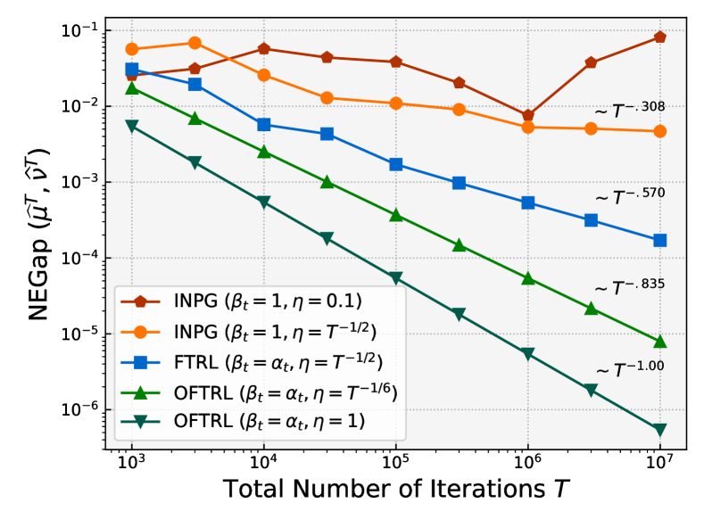
(a) Overall ${\rm NEGap}$

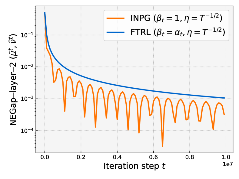
(b) ${\rm NEGap}$ on layer $h=2$

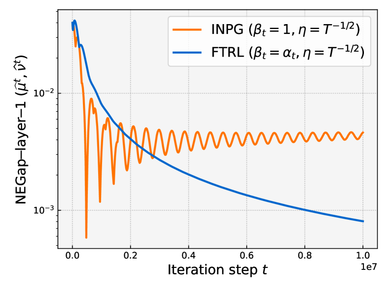
(c) ${\rm NEGap}$ on layer $h=1$

Figure 1: (a) ${\rm NEGap}$ of the final output policies ($y$-axis) against total # iterations $T$ ($x$-axis) on the two-layer example (cf. Appendix H.1) in log-log scale. Each dot represents a different run with its own $(T,\eta)$. The scalings of the form $\sim T^{-\alpha}$ are obtained via best linear fits in the log space. (b,c) Layer-wise ${\rm NEGap}$s ($y$-axis, log-scale) against iteration count $t$ ($x$-axis) for {INPG, FTRL} on a single run with $T=10^{7}$ and $\eta=T^{-1/2}$.

6 Conclusion

This paper provides a unified framework for analyzing a large class of policy optimization algorithms for two-player zero-sum Markov games. Using our framework, we prove new fast convergence rates for the OFTRL algorithm with smooth value updates: $\widetilde{\mathcal{O}}(T^{-5/6})$ for learning Nash Equilibria two-player zero-sum Markov games, which can be further accelerated to $\o(T^{-1})$ by slightly modifying the framework; and $\widetilde{\mathcal{O}}(T^{-3/4})$ for learning Coarse Correlated Equilibria in multi-player general-sum Markov games. We further demonstrate the importance of smooth value updates on a simple numerical example. We believe our work opens up many other interesting directions, such as whether improved rates (e.g. $\widetilde{\mathcal{O}}(T^{-1})$) are available for the unmodified OFTRL algorithm, or further investigation of policy optimization algorithms with eager value updates (such as Independent Natural Policy Gradients). Finally, a limitation of this work is its focus on the full-information setting, and it is an important open question how to generalize our analyses to the sample-based setting.

Appendix A Technical tools

A.1 Properties of $\alpha_{t}^{i}$

Throughout this section, the sequence ${\left\{\beta_{t}^{i}\right\}}_{i\in[t]}$ is defined through sequence ${\left\{\beta_{t}\right\}}_{t\geq 1}$ as in (6), and $\alpha_{t}^{i}$ is its special case with $\beta_{t}=\alpha_{t}$, where ${\left\{\alpha_{t}\right\}}_{t\geq 1}$ is defined in (5). We present some basic algebraic properties of $\alpha_{t}^{i}$ that will be used in later proofs.

Lemma A.0.

Given a sequence $\{\Delta_{h}^{t}\}_{h,t}$ defined by

$$\begin{cases}\Delta_{h}^{t}=\sum_{i=1}^{t}\alpha_{t}^{i}\Delta_{h+1}^{i}+\beta_{t},\\ \Delta_{H+1}^{t}=0,~{}\text{ for all }t,\end{cases}$$ (16)

where $\{\beta_{t}\}$ is non-increasing w.r.t. $t$. Then $\Delta_{h}^{t+1}\leq\Delta_{h}^{t}$ for all $(t,h)\in\mathbb{N}\times[H+1]$.

Proof.

We prove by doing backward induction on $h$. For the base case of induction, notice that the claim is true for $H+1$. Assume the claim is true for $h+1$. At step $h$, we have

$$\Delta_{h}^{t+1} =\sum_{i=1}^{t+1}\alpha_{t+1}^{i}\Delta_{h+1}^{i}+\beta_{t+1}$$

$$=(1-\alpha_{t+1})\sum_{i=1}^{t}\alpha_{t}^{i}\Delta_{h+1}^{i}+\alpha_{t+1}\Delta_{h+1}^{t+1}+\beta_{t+1}$$

$$\leq(1-\alpha_{t+1})\sum_{i=1}^{t}\alpha_{t}^{i}\Delta_{h+1}^{i}+\alpha_{t+1}\sum_{i=1}^{t}\alpha_{t}^{i}\Delta_{h+1}^{i}+\beta_{t}=\Delta_{h}^{t},$$

where the inequality follows from the inductive hypothesis and $\beta_{t+1}\leq\beta_{t}$. ∎

The following lemma is taken from [22].

Lemma A.0.

The sequence $\alpha_{t}^{i}$ satisfies the following:

1. $\sum_{t=i}^{\infty}\alpha_{t}^{i}=1+1/H$ for all $i\geq 1$.

Lemma A.0 (Convolution of $\beta_{T}^{t}$ with decaying sequences).

From general $\{\beta_{t}\}_{t\geq 1}$ sequence, we have that

$$X_{T}\mathrel{\mathop{:}}=\sum_{t=1}^{T}\frac{1}{t}\beta_{T}^{t}\leq\frac{2c_{\beta}\log(T)}{T},~{}~{}~{}\mbox{for $T\geq 2$}.$$

Specifically if $\beta_{t}=\alpha_{t}$, the following holds for all $T\geq 1$:

1. $A_{T}\mathrel{\mathop{:}}=\sum_{t=1}^{T}\alpha_{T}^{t}\cdot\frac{1}{t^{2}}\leq\frac{4}{T}$.

2. $B_{T}\mathrel{\mathop{:}}=\sum_{t=1}^{T}\alpha_{T}^{t}\alpha_{t}\leq\frac{(H+1)^{2}}{H(H+T)}$

3. $C_{T}\mathrel{\mathop{:}}=\sum_{t=1}^{T}\alpha_{T}^{t}\cdot\alpha_{t}^{2}\leq\frac{4H}{T}$.

Proof.

We first prove for the inequality on $X_{T}$ for general $\{\beta_{t}\}_{t\geq 1}$ sequence. We start with showing that $X_{t+1}\leq X_{t},~{}\forall t\geq 1$.

$$X_{t+1} =\sum_{i=1}^{t+1}\frac{1}{i}\beta_{t+1}^{i}=\sum_{i=1}^{t}\frac{1}{i}\beta_{t+1}^{i}+\frac{\beta_{t+1}}{t+1}$$

$$=(1-\beta_{t+1})\sum_{i=1}^{t}\frac{1}{i}\beta_{t}^{i}+\frac{\beta_{t+1}}{t+1}=(1-\beta_{t+1})X_{t}+\frac{\beta_{t+1}}{t+1}$$

$$\Longrightarrow~{}~{} X_{t+1}-X_{t}=\beta_{t+1}{\left(\frac{1}{t+1}-X_{t}\right)}.$$

Since

$$\frac{1}{t+1}-X_{t}=\frac{1}{t+1}-\sum_{i=1}^{t}\frac{1}{i}\beta_{t}^{i}=\sum_{i=1}^{t}\beta_{t}^{i}{\left(\frac{1}{t+1}-\frac{1}{i}\right)}\leq 0,$$

we have that $X_{t+1}-X_{t}\leq 0$.Thus

$$X_{T} \leq\frac{1}{T}\sum_{t=1}^{T}X_{t}=\frac{1}{T}\sum_{t=1}^{T}\sum_{i=1}^{t}\frac{1}{i}\beta_{t}^{i}=\frac{1}{T}\sum_{i=1}^{T}\frac{1}{i}{\left(\sum_{t=i}^{T}\beta_{t}^{i}\right)}\leq\frac{c_{\beta}}{T}\sum_{i=1}^{T}\frac{1}{i}\leq\frac{2c_{\beta}\log(T)}{T}.$$

Now we prove for the specific case where $\beta_{t}=\alpha_{t}$:

1. Note that $A_{1}=1$ and we have the recursive relationship

   $$A_{T+1}=(1-\alpha_{T+1})A_{T}+\alpha_{T+1}\cdot\frac{1}{(T+1)^{2}}$$

   by definition of the sequence $\alpha_{T}^{t}$. In particular this implies $A_{T+1}\leq A_{T}$, since $A_{T}$ is a weighted average of $1/t^{2}\geq 1/(T+1)^{2}$. Therefore we have

   $$\quad A_{T}\leq\frac{1}{T}\sum_{t=1}^{T}A_{t}=\frac{1}{T}\sum_{t=1}^{T}\sum_{s=1}^{t}\alpha_{t}^{s}\cdot\frac{1}{s^{2}}$$

   $$=\frac{1}{T}\sum_{s=1}^{T}\underbrace{\sum_{t=s}^{T}\alpha_{t}^{s}}_{\leq 1+1/H\leq 2}\cdot\frac{1}{s^{2}}\leq\frac{2}{T}\sum_{s=1}^{T}\frac{1}{s^{2}}\leq\frac{2}{T}\sum_{s=1}^{\infty}\frac{1}{s^{2}}\leq\frac{4}{T}.$$

   Above, the step $\sum_{t=s}^{T}\alpha_{t}^{s}\leq\sum_{t=s}^{\infty}\alpha_{t}^{s}=1+1/H$ follows from Lemma A.0.

2. From the definition of $B_{T}$ we have that

   $$B_{T+1}=\sum_{t=1}^{T+1}\alpha_{T+1}^{t}\alpha_{t}=\sum_{t=1}^{T}(1-\alpha_{T+1})\alpha_{T}^{t}\alpha_{t}+\alpha_{T+1}^{2}=(1-\alpha_{T+1}^{t})B_{T}+\alpha_{T+1}$$

   $$\Longrightarrow~{}~{} B_{T+1}=\frac{T}{H+T+1}B_{T}+\frac{(H+1)^{2}}{(H+T+1)^{2}}\leq\frac{T}{H+T+1}B_{T}+\frac{(H+1)^{2}}{(H+T+1)(H+T)}$$

   $$\Longrightarrow~{}~{} {\left(B_{T+1}-\frac{(H+1)^{2}}{H(H+T+1)}\right)}\leq\frac{T}{H+T+1}{\left(B_{T}-\frac{(H+1)^{2}}{H(H+T)}\right)}.$$

   Since $B_{1}=\alpha_{1}^{2}=1\leq\frac{(H+1)^{2}}{H(H+1)}$, we have that $B_{T}\leq\frac{(H+1)^{2}}{H(H+T)}$ via proof by induction.

3. Since $\alpha_{t}\leq 1$, we have that $C_{T}\leq B_{T}$, thus by part (b)

   $$C_{T}\leq B_{T}\leq\frac{(H+1)^{2}}{H(H+T)}\leq\frac{4H}{T}.$$

∎

Consider the sequence ${\left\{w_{t}\right\}}_{t\geq 1}$ defined by (cf. also Example 3.2)

$$w_{t}=\alpha_{t}^{t}/\alpha_{t}^{1}.$$ (17)

Note that we also have $w_{t}=\alpha_{T}^{t}/\alpha_{T}^{1}$ for any $T\geq t$.

Lemma A.0 (Properties of $w_{t}$).

The following holds for all $t\geq 2$:

1. $w_{t}/w_{t-1}=(H+t-1)/(t-1)$.

2. $(\frac{1}{w_{t-1}}-\frac{1}{w_{t}})\sum_{i=1}^{t-1}w_{i}=H/(H+1)$.

Proof.

1. We have

   $$\frac{w_{t}}{w_{t-1}}=\frac{\alpha_{t}}{\alpha_{t-1}(1-\alpha_{t})}=\frac{(H+1)/(H+t)}{(H+1)/(H+t-1)\cdot(t-1)/(H+t)}=\frac{H+t-1}{t-1}.$$

2. We have

   $$\quad{\left(\frac{1}{w_{t-1}}-\frac{1}{w_{t}}\right)}\sum_{i=1}^{t-1}w_{i}=\frac{1}{w_{t-1}}{\left(1-\frac{w_{t-1}}{w_{t}}\right)}\sum_{i=1}^{t-1}w_{i}={\left(1-\frac{w_{t-1}}{w_{t}}\right)}\cdot\frac{1}{\alpha_{t-1}^{t-1}}$$

   $$\stackrel{{\scriptstyle(i)}}{{=}}\frac{H}{H+t-1}\cdot\frac{H+t-1}{H+1}=\frac{H}{H+1}.$$

   Above, (i) used part (a).

∎

A.2 Other technical lemmas

Lemma A.0 (Smoothness of Exponential Weights).

Let $g_{1},g_{2}\in\mathbb{R}^{n}$ and

$$x_{1} =\operatorname*{arg\,max}_{x\in\Delta_{[n]}}\left\langle x,g_{1}\right\rangle-H(x),$$

$$x_{2} =\operatorname*{arg\,max}_{x\in\Delta_{[n]}}\left\langle x,g_{2}\right\rangle-H(x),$$

where $H(x)\mathrel{\mathop{:}}=\sum_{i=1}^{n}x_{i}\log x_{i}$ is the standard entropy functional. Then $\|x_{1}-x_{2}\|_{1}\leq 2\|g_{1}-g_{2}\|_{\infty}$.

Proof.

Since $H$ is $1$-strongly convex in $\|\cdot\|_{1}$ (Pinsker’s inequality), we have that

$$\frac{\|x_{1}-x_{2}\|_{1}^{2}}{2} \leq H(x_{1})-H(x_{2})-\left\langle\nabla H(x_{2}),x_{1}-x_{2}\right\rangle$$

$$=H(x_{1})+\left(\left\langle x_{2},g_{1}\right\rangle-H(x_{2})\right)-\left\langle x_{2},g_{1}\right\rangle-\left\langle\nabla H(x_{2}),x_{1}-x_{2}\right\rangle$$

$$\leq H(x_{1})+\left(\left\langle x_{1},g_{1}\right\rangle-H(x_{1})\right)-\left\langle x_{2},g_{1}\right\rangle-\left\langle\nabla H(x_{2}),x_{1}-x_{2}\right\rangle$$

$$=\left\langle x_{1}-x_{2},g_{1}\right\rangle-\left\langle\nabla H(x_{2}),x_{1}-x_{2}\right\rangle$$

$$=\left\langle x_{1}-x_{2},g_{1}-g_{2}\right\rangle+\left\langle g_{2}-\nabla H(x_{2}),x_{1}-x_{2}\right\rangle$$

$$\leq\left\langle x_{1}-x_{2},g_{1}-g_{2}\right\rangle~{}~{}~{}\textup{(From the optimality of $x_{2}$)}$$

$$\leq\|x_{1}-x_{2}\|_{1}\|g_{1}-g_{2}\|_{\infty},$$

which completes the proof. ∎

Appendix B Bound for regret minimization algorithms

B.1 Projected gradient descent

Algorithm 2 Projected gradient descent

0:  Learning rate $\eta>0$.

1:  Initialize $x_{1}\in\mathcal{X}\subset\mathbb{R}^{d}$.

2:  for $t=1,\ldots,T$ do

3:     Receive loss $g_{t}\in\mathbb{R}^{d}$.

4:     Compute update $y_{t+1}=x_{t}-\eta g_{t}$, $x_{t+1}=\mathcal{P}_{\mathcal{X}}(y_{t+1})$.

The following weighted regret bound for projected gradient descent is standard. For completeness we provide a proof here. For simplicity of notation, denote the diameter of $\mathcal{X}\subset\mathbb{R}^{d}$ by $R$ and $G=\max_{t\in[T]}\|g_{t}\|_{2}$.

Lemma B.0 (Weighted regret bound for projected gradient descent).

For any weights ${\left\{w_{t}\right\}}_{t\geq 1}\in\mathbb{R}_{>0}$ with $w_{t}\leq w_{t+1}$ for all $t\geq 1$, Algorithm 2 achieves

$$\max_{z\in\mathcal{X}}\sum_{t=1}^{T}w_{t}\langle x_{t}-z,g_{t}\rangle\leq\frac{w_{T}}{2\eta}R^{2}+\frac{\eta\sum_{t=1}^{T}w_{t}\cdot G^{2}}{2}.$$

Proof.

By following the standard GD analysis, we first have

$$\langle x_{t}-z,g_{t}\rangle= \frac{1}{\eta}\langle x_{t}-z,x_{t}-y_{t+1}\rangle$$

$$= \frac{1}{2\eta}\left[\|x_{t}-z\|^{2}+\|x_{t}-y_{t+1}\|^{2}-\|z-y_{t+1}\|^{2}\right]$$

$$\leq \frac{1}{2\eta}\left[\|x_{t}-z\|^{2}+\|x_{t}-y_{t+1}\|^{2}-\|z-x_{t+1}\|^{2}\right]$$

$$= \frac{1}{2\eta}\left[\|x_{t}-z\|^{2}-\|z-x_{t+1}\|^{2}+\eta^{2}\|g_{t}\|^{2}\right],$$

where the inequality follows from $z\in\mathcal{X}$ and $x_{t+1}=\mathcal{P}_{\mathcal{X}}(y_{t+1})$. By multiplying both sides with $w_{t}$ and taking summation over $t\in[T]$, we have

$$\sum_{t=1}^{T}w_{t}\langle x_{t}-z,g_{t}\rangle\leq \frac{1}{2\eta}\sum_{t=1}^{T}w_{t}\left[\|x_{t}-z\|^{2}-\|z-x_{t+1}\|^{2}+\eta^{2}\|g_{t}\|^{2}\right]$$

$$= \frac{1}{2\eta}\sum_{t=1}^{T-1}(w_{t+1}-w_{t})\|z-x_{t+1}\|^{2}+w_{1}\|x_{1}-z\|^{2}+\frac{\eta\sum_{t=1}^{T}w_{t}\cdot G^{2}}{2}$$

$$\stackrel{{\scriptstyle(i)}}{{\leq}} \frac{1}{2\eta}\sum_{t=1}^{T-1}(w_{t+1}-w_{t})R^{2}+w_{1}R^{2}+\frac{\eta G^{2}}{2}=\frac{1}{2\eta}w_{T}R^{2}+\frac{\eta\sum_{t=1}^{T}w_{t}\cdot G^{2}}{2},$$

Above, (i) follows as $w_{t+1}\geq w_{t}$. This completes the proof. ∎

B.2 Follow-The-Regularized Leader (FTRL)

In this subsection, we consider the following weighted FTRL algorithm over the probability simplex $\Delta_{[A]}$ with the standard (negative) entropy regularizer $\Phi(x)\mathrel{\mathop{:}}=\sum_{a\in[A]}x(a)\log x(a)$. Below the notation $x_{t}(a)$ denotes the $a$-th entry of $x_{t}$.

Algorithm 3 Weighted FTRL with changing learning rate

0:  Learning rate $\eta>0$; Weights ${\left\{w_{t}\right\}}_{t\geq 1}\subset\mathbb{R}_{>0}$.

1:  Initialize $x_{1}\leftarrow{\mathbf{1}}_{A}/A$ to be the uniform distribution over $[A]$.

2:  for $t=1,\ldots,T$ do

3:     Receive loss $g_{t}\in\mathbb{R}^{A}$.

4:     Compute FTRL update

$$x_{t+1} \leftarrow\operatorname*{arg\,min}_{x\in\Delta_{[A]}}\left\langle x,\sum_{s=1}^{t}w_{s}g_{s}\right\rangle+\frac{w_{t}}{\eta}\Phi(x).$$ (18)

Note that (18) has a closed-form solution via exponential weights:

$$x_{t+1}(a)\propto_{a}\exp{\left(-\frac{\eta}{w_{t}}\sum_{s=1}^{t}w_{s}g_{s}(a)\right)}.$$ (19)

Lemma B.0 (Regret bound of weighted FTRL).

Suppose the weights are non-decreasing: $w_{t+1}\geq w_{t}$ for all $t\geq 1$, and $\max_{t}\|g_{t}\|_{\infty}\leq G$. Then Algorithm 3 achieves weighted regret bound

$$\max_{z\in\Delta_{[A]}}\sum_{t=1}^{T}w_{t}\langle x_{t}-z,g_{t}\rangle\leq\frac{w_{T}}{\eta}\log A+\frac{\eta G^{2}}{2}\sum_{t=1}^{T}w_{t}.$$

Proof.

Applying standard anytime FTRL analysis (see, e.g., Excercise 28.12 in [26]) with loss sequence ${\left\{w_{t}g_{t}\right\}}_{t\geq 1}$ and learning rate ${\left\{\eta/w_{t}\right\}}_{t\geq 1}$, we have that

$$\sum_{t=1}^{T}w_{t}\langle x_{t}-z,g_{t}\rangle \leq\frac{w_{T}(\Phi(x_{1})-\min_{x}\Phi(x))}{\eta}+\sum_{t=1}^{T}w_{t}{\left(\left\langle x_{t}-x_{t+1},g_{t}\right\rangle-\frac{\textup{KL}(x_{t+1}||x_{t})}{\eta}\right)}$$

$$\leq\frac{w_{T}\log A}{\eta}+\sum_{t=1}^{T}{\left(w_{t}\left\langle x_{t}-x_{t+1},g_{t}\right\rangle-\frac{w_{t}\|x_{t}-x_{t+1}\|_{1}^{2}}{2\eta}\right)}~{}~{}~{}~{}\textup{(Pinsker's inequality)}$$

$$\leq\frac{w_{T}\log A}{\eta}+\sum_{t=1}^{T}\frac{w_{t}\eta}{2}\|g_{t}\|_{\infty}^{2}$$

$$\leq\frac{w_{T}\log A}{\eta}+\frac{\eta G^{2}}{2}\sum_{t=1}^{T}w_{t},$$

which completes the proof. ∎

B.3 Optimistic Follow-The-Regularized-Leader (OFTRL)

We consider the following OFTRL algorithm on the probability simplex $\Delta_{[A]}$ with standard (negative) entropy regularizer $\Phi(x)=\sum_{a\in[A]}x(a)\log x(a)$.

Algorithm 4 Anytime OFTRL

0:  Learning rate ${\left\{\eta_{t}\right\}}_{t\geq 1}$.

1:  Initialize $x_{1}\leftarrow{\mathbf{1}}_{A}/A$ to be the uniform distribution over $[A]$.

2:  for $t=1,\ldots,T$ do

3:     Receive loss $g_{t}\in\mathbb{R}^{A}$.

4:     Compute a prediction vector $M_{t+1}\in\mathbb{R}^{A}$ using past observations.

5:     Compute OFTRL update

$$x_{t+1} \leftarrow\operatorname*{arg\,min}_{x\in\Delta_{[A]}}\eta_{t+1}\left\langle x,\sum_{s=1}^{t}g_{s}+M_{t+1}\right\rangle+\Phi(x).$$ (20)

Note that (20) has a closed-form solution via exponential weights:

$$x_{t+1}(a)\propto_{a}\exp{\left(-\eta_{t+1}{\left[\sum_{s=1}^{t}g_{s}(a)+M_{t+1}(a)\right]}\right)}.$$ (21)

The following regret bound for OFTRL follows similarly as standard OFTRL analysis, see, e.g. [39, Lemma 1]. For completeness, we provide a proof here.

Lemma B.0 (Regret bound for OFTRL).

Suppose the learning rates are non-increasing: $\eta_{t}\geq\eta_{t+1}$ for all $t\geq 1$. Then Algorithm 4 achieves the following bound for all $x\in\mathcal{X}$:

$$\sum_{t=1}^{T}\langle x_{t}-x,g_{t}\rangle\leq\frac{\log A}{\eta_{T}}+\sum_{t=1}^{T}\eta_{t}\|g_{t}-M_{t}\|_{\infty}^{2}-\sum_{t=1}^{T-1}\frac{1}{8\eta_{t}}\|x_{t}-x_{t+1}\|_{1}^{2}.$$

Proof.

Consider a fixed $T\geq 1$. Note that Algorithm 4 is equivalent to Algorithm (25) with regularizer $R_{t}(\cdot)\mathrel{\mathop{:}}=(\Phi(\cdot)+\log A)/\eta_{t+1}\geq 0$ for $t\geq 0$, and $R_{T}(\cdot)\mathrel{\mathop{:}}=R_{T-1}(\cdot)$ (Note that the shifting by $\log A$ does not affect the algorithm.)

We first decompose the regret into the following three terms

$$\sum_{t=1}^{T}\langle x_{t}-x,g_{t}\rangle=\sum_{t=1}^{T}\langle q_{t+1}-x,g_{t}\rangle+\sum_{t=1}^{T}\langle x_{t}-q_{t+1},M_{t}\rangle+\sum_{t=1}^{T}\langle x_{t}-q_{t+1},g_{t}-M_{t}\rangle,$$

where ${\left\{q_{t}\right\}}_{t\geq 1}$ is defined in (26). By Lemma B.0, we can upper bound the first two terms by $R_{T}(x)-\min_{x^{\prime}}R_{0}(x^{\prime})+S_{T}\leq R_{T}(x)+S_{T}$ and obtain

$$\sum_{t=1}^{T}\langle x_{t}-x,g_{t}\rangle$$

$$\leq R_{T}(x)+\sum_{t=1}^{T}\left(R_{t-1}(q_{t+1})-R_{t}(q_{t+1})\right)+\sum_{t=1}^{T}\left(\langle x_{t}-q_{t+1},g_{t}-M_{t}\rangle-D_{R_{t-1}}(q_{t+1},x_{t})-D_{R_{t-1}}(x_{t},q_{t})\right)$$

$$\leq R_{T}(x)+\sum_{t=1}^{T}\left(\|x_{t}-q_{t+1}\|_{1}\|g_{t}-M_{t}\|_{\infty}-\frac{1}{2\eta_{t}}\|q_{t+1}-x_{t}\|_{1}^{2}-\frac{1}{2\eta_{t}}\|x_{t}-q_{t}\|_{1}^{2}\right),$$

where the second inequality uses $R_{t-1}\leq R_{t}$ and $R_{t-1}$ is $1/\eta_{t}$ strongly-convex w.r.t. $\|\cdot\|_{1}$. Finally, we conclude the proof by applying Cauchy-Schwarz inequality:

$$\|x_{t}-q_{t+1}\|_{1}\|g_{t}-M_{t}\|_{\infty}-\frac{1}{4\eta_{t}}\|q_{t+1}-x_{t}\|_{1}^{2}\leq\eta_{t}\|g_{t}-M_{t}\|_{\infty}^{2},$$

and triangle inequality

$$-\frac{1}{4\eta_{t}}\|q_{t+1}-x_{t}\|_{1}^{2}-\frac{1}{4\eta_{t}}\|q_{t+1}-x_{t+1}\|_{1}^{2}\leq-\frac{1}{8\eta_{t}}\|x_{t+1}-x_{t}\|_{1}^{2},$$

and the bound $R_{T}(x)\leq\log A/\eta_{T+1}=\log A/\eta_{T}$ for any $x\in\Delta_{[A]}$. ∎

The following lemma bounds the total variation of the iterates in terms of the smoothness of loss vectors and prediction vectors. This can be seen as a generalization of [9, Lemma 3.2] to the case with changing learning rate and arbitrary prediction vectors.

Lemma B.0 (Bounding stability by the smoothness of loss).

Suppose the learning rates are non-increasing: $\eta_{t}\geq\eta_{t+1}$ for all $t\geq 1$. Then the OFTRL algorithm (20) satisfies (understanding $M_{1}\mathrel{\mathop{:}}=0$)

$$\quad\sum_{t=2}^{T}\frac{1}{2\eta_{t}}\left\|{x_{t}-x_{t-1}}\right\|_{1}^{2}\leq\frac{\log A}{\eta_{T}}+\max_{x\in\Delta_{[d]}}\sum_{t=1}^{T-1}\left\langle x_{t}-x,g_{t}\right\rangle+\sum_{t=2}^{T}\left\|{M_{t}-M_{t-1}}\right\|_{\infty}+\left\|{M_{T}}\right\|_{\infty}$$ (22)

$$\leq\frac{2\log A}{\eta_{T}}+\sum_{t=1}^{T-1}\eta_{t}\left\|{g_{t}-M_{t}}\right\|_{\infty}^{2}+\sum_{t=2}^{T}\left\|{M_{t}-M_{t-1}}\right\|_{\infty}+\left\|{M_{T}}\right\|_{\infty}.$$ (23)

In particular, choosing the prediction vector $M_{t}=g_{t-1}$ with $g_{0}\mathrel{\mathop{:}}=0$, and assume $\left\|{g_{t}-g_{t-1}}\right\|_{\infty}\leq G_{t}$ for all $t\geq 1$, we have

$$\begin{aligned} &\quad\sum_{t=2}^{T}\frac{1}{2\eta_{t}}\left\|{x_{t}-x_{t-1}}\right\|_{1}^{2}\leq\frac{2\log A}{\eta_{T}}+\sum_{t=1}^{T-1}\eta_{t}\left\|{g_{t}-g_{t-1}}\right\|_{\infty}^{2}+\sum_{t=2}^{T}\left\|{g_{t-1}-g_{t-2}}\right\|_{\infty}+\left\|{g_{T-1}}\right\|_{\infty}\\ &\leq\frac{2\log A}{\eta_{T}}+\sum_{t=1}^{T-1}(1+\eta_{t}G_{t})\left\|{g_{t}-g_{t-1}}\right\|_{\infty}+\left\|{g_{T-1}}\right\|_{\infty}.\end{aligned}$$ (24)

Proof.

We first prove (22). For any $t\geq 2$, the optimality condition of (20) for $x_{t}$ gives

$$\left\langle\sum_{s=1}^{t-1}g_{s}+M_{t}+\frac{\nabla\Phi(x_{t})}{\eta_{t}},x^{\prime}-x_{t}\right\rangle\geq 0$$

for all $x^{\prime}\in\Delta_{[A]}$. In particular, this holds for $x^{\prime}=x_{t-1}$, from which we get

$$\quad\frac{1}{2\eta_{t}}\left\|{x_{t-1}-x_{t}}\right\|_{1}^{2}\stackrel{{\scriptstyle(i)}}{{\leq}}\frac{1}{\eta_{t}}\textup{KL}(x_{t-1}\|x_{t})\stackrel{{\scriptstyle(ii)}}{{=}}\frac{\Phi(x_{t-1})-\Phi(x_{t})}{\eta_{t}}-\left\langle\frac{\nabla\Phi(x_{t})}{\eta_{t}},x_{t-1}-x_{t}\right\rangle$$

$$\leq\frac{\Phi(x_{t-1})-\Phi(x_{t})}{\eta_{t}}+\left\langle\sum_{s=1}^{t-1}g_{s}+M_{t},x_{t-1}-x_{t}\right\rangle,$$

where (i) is by Pinsker’s inequality, and (ii) is since the KL divergence is the Bregman divergence of $\Phi$. Summing the above over $t=2,\dots,T$ yields

$$\quad\sum_{t=2}^{T}\frac{1}{2\eta_{t}}\left\|{x_{t-1}-x_{t}}\right\|_{1}^{2}$$

$$\leq\underbrace{-\frac{\Phi(x_{T})}{\eta_{T}}}_{\leq\log A/\eta_{T}}+\sum_{t=2}^{T}\underbrace{{\left(\frac{1}{\eta_{t}}-\frac{1}{\eta_{t-1}}\right)}}_{\geq 0}\underbrace{\Phi(x_{t-1})}_{\leq 0}-\left\langle\sum_{s=1}^{T-1}g_{s}+M_{T},x_{T}\right\rangle+\sum_{t=2}^{T}\left\langle g_{t-1}+M_{t}-M_{t-1},x_{t-1}\right\rangle$$

$$\leq\frac{\log A}{\eta_{T}}+\sum_{t=1}^{T-1}\left\langle x_{t},g_{t}\right\rangle-\sum_{t=1}^{T-1}\left\langle x_{T},g_{t}\right\rangle+\left\langle M_{T},x_{T}\right\rangle+\sum_{t=2}^{T}\left\langle M_{t}-M_{t-1},x_{t-1}\right\rangle$$

$$\leq\frac{\log A}{\eta_{T}}+\max_{x\in\Delta_{[d]}}\sum_{t=1}^{T-1}\left\langle x_{t}-x,g_{t}\right\rangle+\sum_{t=2}^{T}\left\|{M_{t}-M_{t-1}}\right\|_{\infty}+\left\|{M_{T}}\right\|_{\infty}.$$

This proves (22). Then, (23) follows by plugging in the regret bound given by Lemma B.0:

$$\max_{x\in\Delta_{[d]}}\sum_{t=1}^{T-1}\left\langle x_{t}-x,g_{t}\right\rangle\leq\frac{\log A}{\eta_{T-1}}+\sum_{t=1}^{T-1}\eta_{t}\left\|{g_{t}-M_{t}}\right\|_{\infty}^{2}\leq\frac{\log A}{\eta_{T}}+\sum_{t=1}^{T-1}\eta_{t}\left\|{g_{t}-M_{t}}\right\|_{\infty}^{2}.$$

Finally, (24) is a direct consequence of (23) by plugging in $M_{t}=g_{t-1}$ and $\left\|{g_{t}-g_{t-1}}\right\|_{\infty}\leq G_{t}$ for all $t\geq 1$. ∎

B.3.1 Auxiliary lemma for OFTRL with general regularizers

Consider an OFTRL algorithm with loss function ${\left\{g_{t}\right\}}_{t\geq 0}\subset\mathbb{R}^{d}$, parameter space $\mathcal{X}\subset\mathbb{R}^{d}$, and convex regularizers $R_{t}:\mathcal{X}\to\mathbb{R}$ for $t\geq 0$:

$$x_{t+1} \leftarrow\operatorname*{arg\,min}_{x\in\mathcal{X}}\left\langle x,\sum_{s=1}^{t}g_{s}+M_{t+1}\right\rangle+R_{t}(x).$$ (25)

Define auxiliary sequence

$$q_{t+1}=\arg\min_{x\in\mathcal{X}}\left\langle x,\sum_{s=1}^{t}g_{s}\right\rangle+R_{t}(x).$$ (26)

Recall the Bregman divergence associated with any convex regularizer $R:\mathcal{X}\to\mathbb{R}$ is given by

$$D_{R}(x,y)\mathrel{\mathop{:}}=R(x)-R(y)-\left\langle\nabla R(y),x-y\right\rangle\geq 0.$$

Lemma B.0 (Auxiliary lemma for OFTRL with general regularizers).

Algorithm (25) achieves the following for any $T\geq 1$ and $x\in\mathcal{X}$:

$$\sum_{t=1}^{T}\langle q_{t+1},g_{t}\rangle+\sum_{t=1}^{T}\langle x_{t}-q_{t+1},M_{t}\rangle\leq\sum_{t=1}^{T}\langle x,g_{t}\rangle+R_{T}(x)-\min_{x^{\prime}\in\mathcal{X}}R_{0}(x^{\prime})+S_{T},$$

where

$$S_{T}\mathrel{\mathop{:}}=\sum_{t=1}^{T}\left(R_{t-1}(q_{t+1})-R_{t}(q_{t+1})\right)-\sum_{t=1}^{T}\left(D_{R_{t-1}}(q_{t+1},x_{t})+D_{R_{t-1}}(x_{t},q_{t})\right).$$

Proof.

We prove the lemma by induction. The above relation holds trivially for $T=0$. Assume the relation holds for $\tau=T-1$. For $\tau=T$, we have

$$\sum_{t=1}^{T}\langle q_{t+1},g_{t}\rangle+\sum_{t=1}^{T}\langle x_{t}-q_{t+1},M_{t}\rangle$$

$$\leq \min_{x\in\mathcal{X}}{\left[\sum_{t=1}^{T-1}\langle x,g_{t}\rangle+R_{T-1}(x)\right]}-\min_{x^{\prime}\in\mathcal{X}}R_{0}(x^{\prime})+S_{T-1}+\langle q_{T+1},g_{T}\rangle+\langle x_{T}-q_{T+1},M_{T}\rangle$$

$$= \sum_{t=1}^{T-1}\langle q_{T},g_{t}\rangle+R_{T-1}(q_{T})-\min_{x^{\prime}\in\mathcal{X}}R_{0}(x^{\prime})$$

$$\qquad+S_{T-1}+\langle q_{T+1},g_{T}\rangle+\langle x_{T}-q_{T+1},M_{T}\rangle\quad\mbox{(definition of $q_{T}$)}$$

$$\leq \sum_{t=1}^{T-1}\langle x_{T},g_{t}\rangle+R_{T-1}(x_{T})-D_{R_{T-1}}(x_{T},q_{T})-\min_{x^{\prime}\in\mathcal{X}}R_{0}(x^{\prime})$$

$$\qquad+S_{T-1}+\langle q_{T+1},g_{T}\rangle+\langle x_{T}-q_{T+1},M_{T}\rangle\quad\mbox{(optimality of $q_{T}$)}$$

$$= \min_{x\in\mathcal{X}}{\left[\langle x,\sum_{t=1}^{T-1}g_{t}+M_{T}\rangle+R_{T-1}(x)\right]}-D_{R_{T-1}}(x_{T},q_{T})-\min_{x^{\prime}\in\mathcal{X}}R_{0}(x^{\prime})$$

$$\qquad+S_{T-1}+\langle q_{T+1},g_{T}-M_{T}\rangle\quad\mbox{(definition of $x_{T}$)}$$

$$\leq \langle q_{T+1},\sum_{t=1}^{T-1}g_{t}+M_{T}\rangle+R_{T-1}(q_{T+1})-D_{R_{T-1}}(q_{T+1},x_{T})$$

$$\qquad-D_{R_{T-1}}(x_{T},q_{T})-\min_{x^{\prime}\in\mathcal{X}}R_{0}(x^{\prime})+S_{T-1}+\langle q_{T+1},g_{T}-M_{T}\rangle\quad\mbox{(optimality of $x_{T}$)}$$

$$= \min_{x\in\mathcal{X}}\langle x,\sum_{t=1}^{T}g_{t}\rangle+R_{T}(x)+(R_{T-1}(q_{T+1})-R_{T}(q_{T+1}))$$

$$\qquad-D_{R_{T-1}}(q_{T+1},x_{T})-D_{R_{T-1}}(x_{T},q_{T})-\min_{x^{\prime}\in\mathcal{X}}R_{0}(x^{\prime})+S_{T-1}\quad\mbox{(definition of $q_{T+1}$)},$$

which completes the induction. ∎

Appendix C Proofs for Section 3.1

In this section we prove Theorem 2. The proof relies on the following two lemmas.

Lemma C.0 (Performance difference for Markov policies).

In two-player zero-sum Markov games, suppose a Markov policy $(\mu,\nu)$ satisfies the following for all $h\in[H+1]$:

$$\max_{s}\max_{\mu^{\dagger}\in\Delta_{\mathcal{A}}}\left({\left[(\mu^{\dagger})^{\top}Q_{h}^{\star}\nu_{h}\right]}(s)-V_{h}^{\star}(s)\right)\leq\varepsilon_{h},$$

$$\max_{s}\max_{\nu^{\dagger}\in\Delta_{\mathcal{B}}}\left(V_{h}^{\star}(s)-{\left[\mu_{h}^{\top}Q_{h}^{\star}\nu^{\dagger}\right]}(s)\right)\leq\varepsilon_{h}.$$

Then we have for all $h\in[H]$ that

$$\max{\left\{\|V_{h}^{\dagger,\nu}-V_{h}^{\star}\|_{\infty},\|V_{h}^{\mu,\dagger}-V_{h}^{\star}\|_{\infty}\right\}}\leq\sum_{h^{\prime}=h}^{H}\varepsilon_{h^{\prime}}.$$

Proof.

We prove by backward induction over $h$. The claim is trivial for $h=H+1$. Suppose the claim holds for step $h+1$. At step $h$,

$$\|V_{h}^{\dagger,\nu}-V_{h}^{\star}\|_{\infty} =\max_{s}{\left|\max_{\mu^{\dagger}\in\Delta_{\mathcal{A}}}{\left[(\mu^{\dagger})^{\top}Q_{h}^{\dagger,\nu}\nu_{h}\right]}(s)-V_{h}^{\star}(s)\right|}$$

$$\leq\max_{s}{\left|\max_{\mu^{\dagger}\in\Delta_{\mathcal{A}}}{\left[(\mu^{\dagger})^{\top}Q_{h}^{\star}\nu_{h}\right]}(s)-V_{h}^{\star}(s)\right|}+\|Q_{h}^{\dagger,\nu}-Q_{h}^{\star}\|_{\infty}$$

$$\leq\varepsilon_{h}+\|Q_{h}^{\dagger,\nu}-Q_{h}^{\star}\|_{\infty}.$$

Notice that

$$\quad\|Q_{h}^{\dagger,\nu}-Q_{h}^{\star}\|_{\infty}\leq\max_{s,a,b}{\left|{\left(r_{h}+\mathbb{P}_{h}V_{h+1}^{\dagger,\nu}\right)}(s,a,b)-{\left(r_{h}+\mathbb{P}_{h}V_{h+1}^{\star}\right)}(s,a,b)\right|}$$

$$\leq\max_{s,a,b}{\left|\mathbb{P}_{h}{\left[V_{h+1}^{\dagger,\nu}-V_{h+1}^{\star}\right]}(s,a,b)\right|}\leq\|V_{h+1}^{\dagger,\nu}-V_{h+1}^{\star}\|_{\infty}\leq\sum_{h^{\prime}=h+1}^{H}\varepsilon_{h^{\prime}}.\quad\textup{(by inductive hypothesis)}$$

Combining the two inequalities we get

$$\|V_{h}^{\dagger,\nu}-V_{h}^{\star}\|_{\infty}\leq\sum_{h^{\prime}=h}^{H}\varepsilon_{h^{\prime}}.$$

This proves the claim for $\|V_{h}^{\dagger,\nu}-V_{h}^{\star}\|_{\infty}$. The same argument also holds for $\|V_{h}^{\mu,\dagger}-V_{h}^{\star}\|_{\infty}$, which completes the proof. ∎

Throughout the rest of this section, we define the following shorthand for the value estimation error:

$$\delta_{h}^{t}\mathrel{\mathop{:}}=\left\|{Q_{h}^{t}-Q_{h}^{\star}}\right\|_{\infty}=\max_{s,a,b}{\left|Q_{h}^{t}(s,a,b)-Q_{h}^{\star}(s,a,b)\right|},$$

where $Q_{h}^{t}$ is the estimated value in Algorithm 1.

Lemma C.0 (Recursion of value estimation).

Algorithm 1 guarantees that for all $(t,h)\in[T]\times[H]$,

$$\delta_{h}^{t}\leq\sum_{i=1}^{t}\beta_{t}^{i}\delta_{h+1}^{i}+{\rm reg}_{h+1}^{t}.$$

Further, suppose that ${\rm reg}_{h}^{t}\leq\overline{\rm reg}_{h}^{t}$ for all $(h,t)\in[H]\times[T]$, where $\overline{\rm reg}_{h}^{t}$ is non-increasing in $t$: $\overline{\rm reg}_{h}^{t}\geq\overline{\rm reg}_{h}^{t+1}$ for all $t\geq 1$. Then we have

$$\delta_{h}^{t}\leq Hc_{\beta}^{H-1}\cdot\frac{1}{t}\sum_{i=1}^{t}\max_{h^{\prime}}\overline{\rm reg}_{h^{\prime}}^{i},$$

where $c_{\beta}$ is defined in (9).

Proof.

Fix $(h,s,a,b)\in[H]\times\mathcal{S}\times\mathcal{A}\times\mathcal{B}$. From the definition of $Q_{h}^{\star}$ we have that

$$Q^{\star}_{h}(s,a,b) =r_{h}(s,a,b)+\max_{\mu_{h+1}}\min_{\nu_{h+1}}\mathbb{P}_{h}{\left[\mu_{h+1}^{\top}Q_{h+1}^{\star}\nu_{h+1}\right]}(s,a,b)$$

$$\leq r_{h}(s,a,b)+\max_{\mu_{h+1}}\mathbb{P}_{h}{\left[\mu_{h+1}^{\top}Q_{h+1}^{\star}{\left(\sum_{i=1}^{t}\beta_{t}^{i}\nu_{h+1}^{i}\right)}\right]}(s,a,b)$$

$$=r_{h}(s,a,b)+\max_{\mu_{h+1}}\sum_{i=1}^{t}\beta_{t}^{i}\mathbb{P}_{h}{\left[\mu_{h+1}^{\top}Q_{h+1}^{\star}\nu_{h+1}^{i}\right]}(s,a,b)$$

$$\leq r_{h}(s,a,b)+\max_{\mu_{h+1}}\sum_{i=1}^{t}\beta_{t}^{i}{\left(\mathbb{P}_{h}{\left[\mu_{h+1}^{\top}Q_{h+1}^{i}\nu_{h+1}^{i}\right]}(s,a,b)+\|Q_{h+1}^{i}-Q^{\star}_{h+1}\|_{\infty}\right)}$$

$$\leq r_{h}(s,a,b)+\sum_{i=1}^{t}\beta_{t}^{i}\mathbb{P}_{h}{\left[(\mu_{h+1}^{i})^{\top}Q_{h+1}^{i}\nu_{h+1}^{i}\right]}(s,a,b)+\sum_{i=1}^{t}\beta_{t}^{i}\delta_{h+1}^{i}+{\rm reg}_{h+1}^{t}$$

$$=Q_{h}^{t}(s,a,b)+\sum_{i=1}^{t}\beta_{t}^{i}\delta_{h+1}^{i}+{\rm reg}_{h+1}^{t}.$$

Above, the last equality is derived from the update rule (3), which implies that

$$Q_{h}^{t}(s,a,b)=\sum_{i=1}^{t}\beta_{t}^{i}{\left(r_{h}+\mathbb{P}_{h}{\left[(\mu_{h+1}^{i})^{\top}Q_{h+1}^{i}\nu_{h+1}^{i}\right]}\right)}(s,a,b).$$

Therefore we have

$$Q^{\star}_{h}(s,a,b)-Q_{h}^{t}(s,a,b)\leq\sum_{i=1}^{t}\beta_{t}^{i}\delta_{h+1}^{i}+{\rm reg}_{h+1}^{t},~{}~{}\forall~{}s,a,b.$$

Apply similar analysis to the min-player, we get

$$Q_{h}^{t}(s,a,b)-Q^{\star}_{h}(s,a,b)\leq\sum_{i=1}^{t}\beta_{t}^{i}\delta_{h+1}^{i}+{\rm reg}_{h+1}^{t},~{}~{}\forall~{}s,a,b.$$

Thus we get

$$\delta_{h}^{t}\leq\sum_{i=1}^{t}\beta_{t}^{i}\delta_{h+1}^{i}+{\rm reg}_{h+1}^{t},$$

which completes the proof of the first inequality in the Lemma. Now consider an auxiliary sequence $\{\Delta_{h}^{t}\}_{h,t}$ defined by

$$\begin{cases}\Delta_{h}^{t}=\sum_{i=1}^{t}\beta_{t}^{i}\Delta_{h+1}^{i}+\overline{\rm reg}_{h+1}^{t},\\ \Delta_{H+1}^{t}=0,~{}\text{ for all }t.\end{cases}$$ (27)

Where $\overline{\rm reg}_{h}^{t}$ is the upperbound of ${\rm reg}_{h}^{t}$ defined in Theorem 2. Observe that $\{\Delta_{h}^{t}\}_{h,t}$ satisfies the following properties

$$\begin{cases}\Delta_{h}^{t}\geq\delta_{h}^{t}\qquad&\text{ (by definition)},\\ \Delta_{h}^{t}\leq\Delta_{h}^{t-1}\quad&\text{ (by Lemma \ref{lem:delta.monotonic})}.\end{cases}$$ (28)

Therefore, to control $\delta_{h}^{t}$, it suffices to bound $\Delta_{h}^{t}\leq\frac{1}{t}\sum_{i=1}^{t}\Delta_{h}^{i}$, which follows from the standard argument in [22]:

$$\frac{1}{t}\sum_{i=1}^{t}\Delta_{h}^{i} =\frac{1}{t}\sum_{i=1}^{t}\sum_{j=1}^{i}\beta_{i}^{j}\Delta_{h+1}^{j}+\frac{1}{t}\sum_{i=1}^{t}\overline{\rm reg}_{h+1}^{i}$$

$$\leq\frac{1}{t}\sum_{j=1}^{t}{\left(\sum_{i=j}^{t}\beta_{i}^{j}\right)}\Delta_{h+1}^{j}+\frac{1}{t}\sum_{i=1}^{t}\overline{\rm reg}_{h+1}^{i}$$

$$\leq c_{\beta}\cdot\frac{1}{t}\sum_{i=1}^{t}\Delta_{h+1}^{i}+\frac{1}{t}\sum_{i=1}^{t}\overline{\rm reg}_{h+1}^{i}$$

$$\leq c_{\beta}^{2}\cdot\frac{1}{t}\sum_{i=1}^{t}\Delta_{h+2}^{i}+c_{\beta}\cdot\frac{1}{t}\sum_{i=1}^{t}\overline{\rm reg}_{h+2}^{i}+\frac{1}{t}\sum_{i=1}^{t}\overline{\rm reg}_{h+1}^{i}$$

$$\leq\cdots$$

$$\leq{\left(\sum_{h^{\prime}=h+1}^{H}c_{\beta}^{h^{\prime}-h}\right)}\cdot\frac{1}{t}\sum_{i=1}^{t}\max_{1\leq h^{\prime}\leq H}\overline{\rm reg}_{h^{\prime}}^{i}$$

$$\leq Hc_{\beta}^{H-1}\cdot\frac{1}{t}\sum_{i=1}^{t}\max_{1\leq h^{\prime}\leq H}\overline{\rm reg}_{h^{\prime}}^{i}.$$

Above, the last step used the fact that $c_{\beta}\geq 1$. This completes the proof of the second inequality in the Lemma. ∎

We are now ready to prove the main theorem.

Proof of Theorem 2.

Fix any $(h,s)\in[H]\times\mathcal{S}$. We first give a bound for $\max_{\mu^{\dagger}\in\Delta_{\mathcal{A}},\nu^{\dagger}\in\Delta_{\mathcal{B}}}{\left[(\mu^{\dagger})^{\top}Q_{h}^{\star}\widehat{\nu}_{h}^{T}-{\left(\widehat{\mu}_{h}^{T}\right)}^{\top}Q_{h}^{\star}\nu^{\dagger}\right]}(s)$, i.e. the per-state duality gap of $(\widehat{\mu}^{T},\widehat{\nu}^{T})$ with respect to $Q_{h}^{\star}$. We have

$$\quad\max_{\mu^{\dagger}\in\Delta_{\mathcal{A}},\nu^{\dagger}\in\Delta_{\mathcal{B}}}{\left[(\mu^{\dagger})^{\top}Q_{h}^{\star}\widehat{\nu}_{h}^{T}-{\left(\widehat{\mu}_{h}^{T}\right)}^{\top}Q_{h}^{\star}\nu^{\dagger}\right]}(s)$$

$$=\max_{\mu^{\dagger}\in\Delta_{\mathcal{A}},\nu^{\dagger}\in\Delta_{\mathcal{B}}}\sum_{t=1}^{T}\beta_{T}^{t}{\left[(\mu^{\dagger})^{\top}Q_{h}^{\star}\nu_{h}^{t}-{\left(\mu_{h}^{t}\right)}^{\top}Q_{h}^{\star}\nu^{\dagger}\right]}(s)$$

$$\leq\underbrace{\max_{\mu^{\dagger}\in\Delta_{\mathcal{A}},\nu^{\dagger}\in\Delta_{\mathcal{B}}}\sum_{t=1}^{T}\beta_{T}^{t}{\left[(\mu^{\dagger})^{\top}Q_{h}^{t}\nu_{h}^{t}-{\left(\mu_{h}^{t}\right)}^{\top}Q_{h}^{t}\nu^{\dagger}\right]}(s)}_{{\rm reg}_{\mu,h}^{T}(s)+{\rm reg}_{\nu,h}^{T}(s)}+2\sum_{t=1}^{T}\beta_{T}^{t}\delta_{h}^{t}$$

$$\leq 2\overline{\rm reg}_{h}^{T}+2Hc_{\beta}^{H-1}\sum_{t=1}^{T}\beta_{T}^{t}\cdot\frac{1}{t}\sum_{i=1}^{t}\max_{h^{\prime}}\overline{\rm reg}_{h^{\prime}}^{i}~{}~{}~{}\textup{(Lemma \ref{lemma:recursion-of-value-estimation})}$$

$$\leq 2\overline{\rm reg}_{h}^{T}+2Hc_{\beta}^{H-1}{\left(\sum_{t=1}^{T}\frac{1}{t}\beta_{T}^{t}\right)}{\left(\sum_{i=1}^{T}\max_{h^{\prime}}\overline{\rm reg}_{h^{\prime}}^{i}\right)}.$$

Apply Lemma A.0 into the above inequality, we get that

$$\max_{\mu^{\dagger}\in\Delta_{\mathcal{A}},\nu^{\dagger}\in\Delta_{\mathcal{B}}}{\left[(\mu^{\dagger})^{\top}Q_{h}^{\star}\widehat{\nu}_{h}^{T}\!-\!{\left(\widehat{\mu}_{h}^{T}\right)}^{\top}Q_{h}^{\star}\nu^{\dagger}\right]}(s)\leq 2\overline{\rm reg}_{h}^{T}+4Hc_{\beta}^{H}\log T\cdot\frac{1}{T}\sum_{t=1}^{T}\max_{h^{\prime}}\overline{\rm reg}_{h^{\prime}}^{t}.$$

Since

$$\max_{\mu^{\dagger}\!\in\!\Delta_{\mathcal{A}}}\left({\left[(\mu^{\dagger})^{\!\!\top}\!Q_{h}^{\star}\widehat{\nu}^{T}_{h}\right]}(s)\!-\!V_{h}^{\star}(s)\right),\max_{\nu^{\dagger}\!\in\!\Delta_{\mathcal{B}}}\left(V_{h}^{\star}(s)\!-\!{\left[(\widehat{\mu}_{h}^{T})^{\top}Q_{h}^{\star}\nu^{\dagger}\right]}(s)\right)\!\leq\!\!\max_{\mu^{\dagger}\!\in\!\Delta_{\mathcal{A}},\nu^{\dagger}\!\in\!\Delta_{\mathcal{B}}}{\left[(\mu^{\dagger})^{\!\!\top}\!Q_{h}^{\star}\widehat{\nu}_{h}^{T}\!-\!{\left(\widehat{\mu}_{h}^{T}\right)}^{\!\!\top}\!Q_{h}^{\star}\nu^{\dagger}\right]}(s),$$

by applying Lemma C.0 and the preceding per-state duality gap bound, we have

$$\quad{\rm NEGap}(\widehat{\mu}^{T},\widehat{\nu}^{T})={\left(V_{1}^{\dagger,\widehat{\nu}^{T}}(s_{1})-V_{1}^{\star}(s_{1})\right)}+{\left(V_{1}^{\star}(s_{1})-V_{1}^{\widehat{\mu}^{T},\dagger}(s_{1})\right)}$$

$$\leq 2\sum_{h=1}^{H}\max_{s}\max_{\mu^{\dagger}\in\Delta_{\mathcal{A}},\nu^{\dagger}\in\Delta_{\mathcal{B}}}{\left[(\mu^{\dagger})^{\top}Q_{h}^{\star}\widehat{\nu}_{h}^{T}\!-\!{\left(\widehat{\mu}_{h}^{T}\right)}^{\top}Q_{h}^{\star}\nu^{\dagger}\right]}(s)$$

$$\leq 2\sum_{h=1}^{H}{\left(2\overline{\rm reg}_{h}^{T}+4Hc_{\beta}^{H}\log T\cdot\frac{1}{T}\sum_{t=1}^{T}\max_{h^{\prime}}\overline{\rm reg}_{h^{\prime}}^{t}\right)}$$

$$\leq 4H\max_{h}\overline{\rm reg}_{h}^{T}+8H^{2}c_{\beta}^{H}\log T\cdot\frac{1}{T}\sum_{t=1}^{T}\max_{h^{\prime}}\overline{\rm reg}_{h^{\prime}}^{t}.$$

This completes the proof. ∎

Appendix D Algorithm details and proofs for Section 3.2

D.1 Nash V-Learning (full-information version)

The full description of Nash V-Learning (Example 3.2) using V updates is presented in Algorithm 5.

Algorithm 5 Nash V-learning (full-information version)

  Require: Learning rate $\{\alpha_{t}\}_{t\geq 1}$ in (5) and corresponding $\{w_{t}\}_{t\geq 1}$ (cf. Example 3.2); $\eta>0$.

  Initialize: Set $V_{h}^{0}(s)=H-h+1$ for all $(h,s)\in[H]\times\mathcal{S}$.

  for $t=1,\ldots,T$ do

     for $h=H,\ldots,1$ do

        Update policy for all $s\in\mathcal{S}$ (understanding $w_{0}\mathrel{\mathop{:}}=1$):

$$\begin{split}\mu_{h}^{t}(a|s)&\propto_{a}\exp{\left(\frac{\eta}{w_{t-1}}\sum_{i=1}^{t-1}w_{i}{\left[{\left(r_{h}+\mathbb{P}_{h}V_{h+1}^{i}\right)}\nu_{h}^{i}\right]}(s,a)\right)}\\ \nu_{h}^{t}(a|s)&\propto_{b}\exp{\left(-\frac{\eta}{w_{t-1}}\sum_{i=1}^{t-1}w_{i}{\left[{\left(r_{h}+\mathbb{P}_{h}V_{h+1}^{i}\right)}^{\top}\mu_{h}^{i}\right]}(s,b)\right)}.\end{split}$$ (29)

        Update V value for all $s\in\mathcal{S}$:

$$V_{h}^{t}(s)\leftarrow(1-\alpha_{t})V_{h}^{t-1}(s)+\alpha_{t}{\left[{\left(\mu_{h}^{t}\right)}^{\top}{\left(r_{h}+\mathbb{P}_{h}V_{h+1}^{t}\right)}\nu_{h}^{t}\right]}(s).$$ (30)

Proposition D.0 (Equivalence between V update and Q update).

Nash V-learning (full-information version) in Algorithm 5 is equivalent to Algorithm 1 with the ${\sf MatrixGameAlg}$ as weighted FTRL (10).

Proof.

It suffices to show that, for the Q value defined in (3) and the V value defined in (30), the following holds for all $(h,s,a,b)$ and all $t\in[T]$:

$$Q_{h}^{t}(s,a,b)={\left[r_{h}+\mathbb{P}_{h}V_{h+1}^{t}\right]}(s,a,b).$$ (31)

Since $\alpha_{1}=1$, it is not hard to verify that

$$Q_{h}^{1}(s,a,b)={\left[r_{h}+\mathbb{P}_{h}V_{h+1}^{1}\right]}(s,a,b),$$

We now prove by induction on both $t$ and $h$. Given that $Q_{h}^{1}(s,a,b)={\left[r_{h}+\mathbb{P}_{h}V_{h+1}^{1}\right]}(s,a,b)$, it is not hard to verify that $Q_{H}^{t}(s,a,b)=r_{H}(s,a,b),~{}\forall~{}k\geq 0$. We assume that (31) holds for $(t-1,h)$ and $(t,h+1)$, then for $(t,h)$, from (3)

$$\quad Q_{h}^{t}(s,a,b)=(1-\alpha_{t})Q_{h}^{t-1}(s,a,b)+\alpha_{t}{\left(r_{h}+\mathbb{P}_{h}[(\mu_{h+1}^{t})^{\top}Q_{h+1}^{t}\nu_{h+1}^{t}]\right)}(s,a,b)$$

$$\leq(1\!-\!\alpha_{t}){\left[r_{h}\!+\!\mathbb{P}_{h}V_{h+1}^{t-1}\right]}(s,a,b)+\alpha_{t}{\left(r_{h}\!+\!\mathbb{P}_{h}{\left[(\mu_{h+1}^{t})^{\top}{\left(r_{h+1}\!+\!\mathbb{P}_{h+1}V_{h+2}\right)}\nu_{h+1}^{t}\right]}\right)}(s,a,b)$$

(inductive hypothesis)

$$={\left[r_{h}+\mathbb{P}_{h}\left((1-\alpha_{t})V_{h+1}^{t-1}+\alpha_{t}(\mu_{h+1}^{t})^{\top}{\left(r_{h+1}\!+\!\mathbb{P}_{h+1}V_{h+2}\right)}\nu_{h+1}^{t}\right)\right]}(s,a,b)$$

$$={\left[r_{h}+\mathbb{P}_{h}V_{h+1}^{t}\right]}(s,a,b)~{}~{}\textup{(from \eqref{eq:V-update})},$$

which completes the proof by induction. ∎

Lemma D.0 (Per-state regret bound for Nash V-learning).

Algorithm 5 achieves the following per-state regret bound:

$${\rm reg}_{h}^{t}\leq\frac{(H+1)\log(A\vee B)}{\eta t}+\frac{\eta H^{2}}{2},~{}~{}\forall h\in[H],t\geq 1.$$

Proof.

Fix any $(h,s)$. Note that the update of ${\left\{\mu^{t}_{h}(\cdot|s)\right\}}_{t\geq 1}$ in (29) is equivalent to the weighted FTRL algorithm (Algorithm 3) with loss vectors $g_{i}=-{\left[Q_{h}^{i}\nu_{h}^{i}\right]}(s)$. Thus by Lemma B.0 we get for any $t\geq 1$ that

$$\max_{\mu^{\dagger}\in\Delta_{\mathcal{A}}}\sum_{i=1}^{t}w_{i}\left\langle\mu^{\dagger}-\mu_{h}^{i}(\cdot|s),{\left[Q_{h}^{i}\nu_{h}^{i}\right]}(s,\cdot)\right\rangle\leq\frac{w_{t}}{\eta}\log A+\frac{\eta H^{2}}{2}\sum_{i=1}^{t}w_{i}.$$

Further, recalling $\alpha_{t}^{i}=w_{i}\cdot\alpha_{t}^{1}$ for $1\leq i\leq t$, we have

$$\quad{\rm reg}_{h,\mu}^{t}\leq\alpha_{t}^{1}{\left(\frac{w_{t}}{\eta}\log A+\frac{\eta H^{2}}{2}\sum_{i=1}^{t}w_{i}\right)}=\frac{\alpha_{t}^{1}w_{t}}{\eta}\log A+\frac{\eta H^{2}}{2}\sum_{i=1}^{t}\alpha_{t}^{i}$$

$$=\frac{\alpha_{t}}{\eta}\log A+\frac{\eta H^{2}}{2}\leq\frac{(H+1)\log A}{\eta t}+\frac{\eta H^{2}}{2}.$$

The similar bound also holds for ${\rm reg}_{h,\nu}^{t}$, and thus we have that

$${\rm reg}_{h}^{t}\leq\frac{(H+1)\log(A\vee B)}{\eta t}+\frac{\eta H^{2}}{2}.$$

∎

Proposition D.0 (Guarantee of Nash V-Learning).

Algorithm 5 achieves

$${\rm NEGap}(\widehat{\mu}^{T},\widehat{\nu}^{T})\leq 14\eta H^{4}\log(T)+\frac{104\log(A\vee B)\log(T)^{2}H^{3}}{\eta T}.$$

Specifically, choosing $\eta=\frac{4}{\sqrt{HT}}$, we have

$${\rm NEGap}(\widehat{\mu}^{T},\widehat{\nu}^{T})\leq\frac{82\log(A\vee B)\log(T)^{2}H^{7/2}}{\sqrt{T}}.$$

Proof.

From Lemma D.0, we can take $\overline{\rm reg}_{h}^{t}$ as $\overline{\rm reg}_{h}^{t}=\frac{(H+1)\log(A\vee B)}{\eta t}+\frac{\eta H^{2}}{2}$. Then from Theorem 2, we have

$$\quad{\rm NEGap}(\widehat{\mu}^{T},\widehat{\nu}^{T})\leq 4H\max_{h}\overline{\rm reg}_{h}^{T}+8H^{2}{\left(1+\frac{1}{H}\right)}^{H}\log(T)\cdot\frac{1}{T}\sum_{t=1}^{T}\max_{h}\overline{\rm reg}_{h}^{t}$$

$$\leq 4H{\left(\frac{(H+1)\log(A\vee B)}{\eta T}+\frac{\eta H^{2}}{2}\right)}+24H^{2}\log(T)\cdot\frac{1}{T}\sum_{t=1}^{T}{\left(\frac{(H+1)\log(A\vee B)}{\eta t}+\frac{\eta H^{2}}{2}\right)}$$

$$\leq 14\eta H^{4}\log(T)+24H^{2}\log(T)\cdot\frac{1}{T}\sum_{t=1}^{T}\frac{(H+1)\log(A\vee B)}{\eta t}+\frac{8H^{2}\log(A\vee B)}{\eta T}$$

$$\leq 14\eta H^{4}\log(T)+\frac{104\log(A\vee B)\log(T)^{2}H^{3}}{\eta T}.$$

Thus, choosing $\eta=\frac{4}{\sqrt{HT}}$, we get

$${\rm NEGap}(\widehat{\mu}^{T},\widehat{\nu}^{T})\leq\frac{82\log(A\vee B)\log(T)^{2}H^{7/2}}{\sqrt{T}}.$$

∎

D.2 GDA-Critic

The full description of GDA-Critic (Example 3.2) using V updates is presented in Algorithm 6.

Algorithm 6 GDA-Critic

  Require: Learning rate $\{\alpha_{t}\}_{t\geq 1}$ (defined in (5)), and $\eta>0$.

  Initialize: set $V_{h}^{0}(s)=H-h+1$ and $\mu^{0}(\cdot|s),\nu^{0}(\cdot|s)$ to be uniform for all $(h,s)\in[H]\times\mathcal{S}$.

  for $t=1,\ldots,T$ do

     for $h=H,\ldots,1$ do

        Update policy for all $s\in\mathcal{S}$:

$$\begin{split}\mu_{h}^{t}(\cdot|s)&\leftarrow\mathcal{P}_{\Delta_{\mathcal{A}}}{\left(\mu_{h}^{t-1}(\cdot|s)+\eta{\left[{\left(r_{h}+\mathbb{P}_{h}V_{h+1}^{t-1}\right)}\nu_{h}^{t-1}\right]}(s,\cdot,b)\right)}\\ \nu_{h}^{t}(\cdot|s)&\leftarrow\mathcal{P}_{\Delta_{\mathcal{B}}}{\left(\nu_{h}^{t-1}(\cdot|s)-\eta{\left[{\left(r_{h}+\mathbb{P}_{h}V_{h+1}^{t-1}\right)}^{\top}\mu_{h}^{t-1}\right]}(s,a,\cdot)\right)}\\ \end{split}$$ (32)

        Update V value for all $s\in\mathcal{S}$:

$$V_{h}^{t}(s)\leftarrow(1-\alpha_{t})V_{h}^{t-1}(s)+\alpha_{t}{\left[{\left(\mu_{h}^{t}\right)}^{\top}{\left(r_{h}+\mathbb{P}_{h}V_{h+1}^{t}\right)}\nu_{h}^{t}\right]}(s).$$

Similar as Proposition D.0 (with the same proof), the following equivalence between Q updates and V updates also holds for GDA-Critic.

Proposition D.0 (Equivalence between Q updates and V updates for GDA-Critic).

Algorithm 6 is equivalent to our algorithm framework (Algorithm 1) with the ${\sf MatrixGameAlg}$ instantiated as (11).

Lemma D.0 (Per-state regret bound for GDA-Critic).

Algorithm 6 achieves the following per-state regret bound:

$${\rm reg}_{h}^{t}\leq\frac{2(H+1)}{\eta t}+\frac{\eta(A\vee B)H^{2}}{2}.$$

Proof.

Fix any $(h,s)$ and $t\geq 1$. We apply Lemma B.0 to the projected gradient descent (or ascent) update (32), with weights $w_{i}=\alpha_{t}^{i}$ and loss vectors $g_{i}$’s $-{\left[Q_{h}^{i}\nu_{h}^{i}\right]}(s)$ or ${\left[{\left(Q_{h}^{i}\right)}^{\top}\mu_{h}^{i}\right]}(s)$ respectively. For the gradient ascent update for $\mu_{h}^{t}(\cdot|s)$, we get

$${\rm reg}_{h,\mu}^{t}(s) \leq\frac{\alpha_{t}^{t}}{2\eta}\cdot 4+\frac{\eta{\left(\sum_{i=1}^{t}\alpha_{t}^{i}\right)}AH^{2}}{2}=\frac{2}{\eta}\frac{H+1}{H+t}+\frac{\eta AH^{2}}{2}$$

$${\rm reg}_{h,\nu}^{t}(s) \leq\frac{\alpha_{t}^{t}}{2\eta}\cdot 4+\frac{\eta{\left(\sum_{t=1}^{T}\alpha_{t}^{i}\right)}BH^{2}}{2}=\frac{2}{\eta}\frac{H+1}{H+t}+\frac{\eta BH^{2}}{2}$$

$$\Longrightarrow~{}~{}{\rm reg}_{h}^{t} \leq\frac{2(H+1)}{\eta t}+\frac{\eta(A\vee B)H^{2}}{2}.$$

∎

Proposition D.0 (Guarantee of GDA-Critic).

Algorithm 6 achieves

$${\rm NEGap}(\widehat{\mu}^{T},\widehat{\nu}^{T})\leq 14\eta(A\vee B)H^{4}\log(T)+\frac{208\log(T)^{2}H^{3}}{\eta T}.$$

Specifically, picking $\eta=\frac{4}{\sqrt{(A\vee B)HT}}$ yields

$${\rm NEGap}(\widehat{\mu}^{T},\widehat{\nu}^{T})\leq\frac{108\log(T)^{2}\sqrt{A\vee B}H^{7/2}}{\sqrt{T}}.$$

Proof.

From Lemma D.0, we can take $\overline{\rm reg}_{h}^{t}$ as $\frac{2(H+1)}{\eta t}+\frac{\eta(A\vee B)H^{2}}{2}$, then from Theorem 2

$$\quad{\rm NEGap}(\widehat{\mu}^{T},\widehat{\nu}^{T})\leq 4H\max_{h}\overline{\rm reg}_{h}^{T}+8H^{2}{\left(1+\frac{1}{H}\right)}^{H}\log(T)\cdot\frac{1}{T}\sum_{t=1}^{T}\max_{h}\overline{\rm reg}_{h}^{t}$$

$$\leq 4H{\left(\frac{2(H+1)}{\eta T}+\frac{\eta(A\vee B)H^{2}}{2}\right)}+24H^{2}\log(T)\cdot\frac{1}{T}\sum_{t=1}^{T}{\left(\frac{2(H+1)}{\eta t}+\frac{\eta(A\vee B)H^{2}}{2}\right)}$$

$$\leq 14\eta(A\vee B)H^{4}\log(T)+48H^{2}\log(T)\cdot\frac{1}{T}\sum_{t=1}^{T}\frac{(H+1)}{\eta t}+\frac{16H^{2}}{\eta T}$$

$$\leq 14\eta(A\vee B)H^{4}\log(T)+\frac{208\log(T)^{2}H^{3}}{\eta T}.$$

Thus, pick $\eta=\frac{4}{(A\vee B)\sqrt{HT}}$, we get

$${\rm NEGap}(\widehat{\mu}^{T},\widehat{\nu}^{T})\leq\frac{108\log(T)^{2}\sqrt{A\vee B}H^{7/2}}{\sqrt{T}}.$$

∎

D.3 Nash Q-Learning (full-information version)

The Nash Q-Learning algorithm (Example 3.2) is described in Algorithm 7.

Algorithm 7 Nash Q-Learning

  Require: Learning rate (For Nash Q-learning) $\{\beta_{t}=\alpha_{t}\}$;

  Initialize: $Q_{h}^{0}(s,a,b)\leftarrow H-h+1$ for all $(h,s,a,b)$.

  for $k=1,\dots,K$ do

     for $h=H,\dots,1$ do

        Update policy for all $s\in\mathcal{S}$:

$$(\mu_{h}^{t}(\cdot|s),\nu_{h}^{t}(\cdot|s))\leftarrow{\sf MatrixNE}(Q_{h}^{t-1}(s,\cdot,\cdot)).$$ (33)

        Update Q value for all $(s,a,b)\in\mathcal{S}\times\mathcal{A}\times\mathcal{B}$:

$$Q_{h}^{t}(s,a,b)\leftarrow(1-\alpha_{t})Q_{h}^{t-1}(s,a,b)+\alpha_{t}{\left(r_{h}+\mathbb{P}_{h}[(\mu_{h+1}^{t})^{\top}Q_{h+1}^{t}\nu_{h+1}^{t}]\right)}(s,a,b).$$

Lemma D.0 (Per-state regret bound for Nash Q-Learning).

Algorithm 7 achieves the following per-state regret bound:

$${\rm reg}_{h}^{t}\leq\frac{(H+1)^{2}}{H+t},~{}~{}~{}\forall~{}h\in[H],~{}t\geq 1.$$

Proof.

We have

$${\rm reg}_{h,\mu}^{t}(s) =\max_{\mu^{\dagger}\in\Delta_{\mathcal{A}}}\sum_{i=1}^{t}\alpha_{t}^{i}\left\langle\mu^{\dagger}-\mu_{h}^{i}(\cdot|s),{\left[Q_{h}^{i}\nu_{h}^{i}\right]}(s,\cdot)\right\rangle$$

$$=\max_{\mu^{\dagger}\in\Delta_{\mathcal{A}}}\sum_{i=1}^{t}\alpha_{t}^{i}\left\langle\mu^{\dagger}-\mu_{h}^{i}(\cdot|s),{\left[Q_{h}^{i-1}\nu_{h}^{i}\right]}(s,\cdot)\right\rangle+\sum_{i=1}^{t}\alpha_{t}^{i}\|Q_{h}^{i}-Q_{h}^{i-1}\|_{\infty}$$

$$\leq\sum_{i=1}^{t}\alpha_{t}^{i}\underbrace{\max_{\mu^{\dagger}\in\Delta_{\mathcal{A}}}\left\langle\mu^{\dagger}-\mu_{h}^{i}(\cdot|s),{\left[Q_{h}^{i-1}\nu_{h}^{i}\right]}(s,\cdot)\right\rangle}_{=0\textup{ from \eqref{eq:Nash-Q-mu-nu-update}}}+\sum_{i=1}^{t}\alpha_{t}^{i}\|Q_{h}^{i}-Q_{h}^{i-1}\|_{\infty}$$

$$=\sum_{i=1}^{t}\alpha_{t}^{i}\|Q_{h}^{i}-Q_{h}^{i-1}\|_{\infty}.$$

The same bound also holds for ${\rm reg}_{h,\nu}^{t}(s)$, thus

$${\rm reg}_{h}^{t}\leq\sum_{i=1}^{t}\alpha_{t}^{i}\|Q_{h}^{i}-Q_{h}^{i-1}\|_{\infty}.$$

Since

$$Q_{h}^{i}(s,a,b)=(1-\alpha_{i})Q_{h}^{i-1}(s,a,b)+\alpha_{i}{\left(r_{h}+\mathbb{P}_{h}[(\mu_{h+1}^{i})^{\top}Q_{h+1}^{i}\nu_{h+1}^{i}]\right)}(s,a,b)$$

$$\Longrightarrow |Q_{h}^{i}(s,a,b)-Q_{h}^{i-1}(s,a,b)|\leq\alpha_{i}\|Q_{h}^{i-1}-{\left({\left(r_{h}+\mathbb{P}_{h}[(\mu_{h+1}^{i})^{\top}Q_{h+1}^{i}\nu_{h+1}^{i}]\right)}\right)}\|_{\infty}\leq\alpha_{i}H$$

$$\Longrightarrow \|Q_{h}^{i}-Q_{h}^{i-1}\|_{\infty}\leq\alpha_{i}H,$$

substituting this into the above equations we have that

$${\rm reg}_{h}^{t}\leq H\sum_{i=1}^{t}\alpha_{t}^{i}\alpha_{i}\leq\frac{(H+1)^{2}}{H+t}~{}~{}\textup{(From Lemma \ref{lemma:alpha-convolution} (b))},$$

which completes the proof. ∎

Proposition D.0 (Guarantee for Nash Q-Learning).

Algorithm 7 achieves

$${\rm NEGap}(\widehat{\mu}^{T},\widehat{\nu}^{T})\leq\frac{112\log(T)^{2}H^{4}}{T}.$$

Proof.

From Theorem 2 and Lemma D.0 we have that

$$\quad{\rm NEGap}(\widehat{\mu}^{T},\widehat{\nu}^{T})\leq 4H\max_{h}\overline{\rm reg}_{h}^{T}+8H^{2}{\left(1+\frac{1}{H}\right)}^{H}\log(T)\cdot\frac{1}{T}\sum_{t=1}^{T}\max_{h}\overline{\rm reg}_{h}^{t}$$

$$\leq 4H\frac{(H+1)^{2}}{H+T}+24H^{2}\log(T)\cdot\frac{1}{T}\sum_{t=1}^{T}\frac{(H+1)^{2}}{H+t}\leq\frac{112\log(T)^{2}H^{4}}{T}.$$

∎

D.4 Nash Policy Iteration

Algorithm 8 Nash Policy Iteration (Nash-PI)

  Initialize: $Q_{h}^{0}(s,a,b)\leftarrow H-h+1$ for all $(h,s,a,b)$.

  for $t=1,\dots,T$ do

     for $h=H,\dots,1$ do

        Update policy for all $s\in\mathcal{S}$:

$$(\mu_{h}^{t}(\cdot|s),\nu_{h}^{t}(\cdot|s))\leftarrow{\sf MatrixNE}(Q_{h}^{t-1}(s,\cdot,\cdot)).$$

        Update Q value for all $(s,a,b)\in\mathcal{S}\times\mathcal{A}\times\mathcal{B}$:

$$Q_{h}^{t}(s,a,b)\leftarrow{\left[r_{h}+\mathbb{P}_{h}[(\mu_{h+1}^{t})^{\top}Q_{h+1}^{t}\nu_{h+1}^{t}]\right]}(s,a,b).$$ (34)

The full description of Nash Policy Iteration (Nash-PI, Example 3.2) is presented in Algorithm 8.

Note that from (34), we have that $Q_{h}^{k}$ equals to $Q_{h}^{\mu^{k}\times\nu^{k}}$. Based on this observation, we have the following lemma.

Lemma D.0 (Exact learning of Q functions).

For Algorithm 8, we have for any $h\in[H]$ and $t\geq H-h+1$ that

$$Q_{h}^{t}(s,a,b)=Q_{h}^{\star}(s,a,b),~{}~{}\forall~{}(s,a,b)\in\mathcal{S}\times\mathcal{A}\times\mathcal{B}.$$

Proof.

We prove this by backward induction over $h$. For $h=H$, we have that

$$Q_{H}^{t}(s,a,b)=r_{H}(s,a,b),~{}~{}\forall t\geq 1.$$

Assume that for $h+1$, the condition holds, then for time horizon $h$ and iteration step $t\geq H-h+1$, we have that

$$Q_{h}^{t}(s,a,b) ={\left[r_{h}+\mathbb{P}_{h}[(\mu_{h+1}^{t})^{\top}Q_{h+1}^{t}\nu_{h+1}^{t}]\right]}(s,a,b)$$

$$={\left[r_{h}+\mathbb{P}_{h}[(\mu_{h+1}^{t})^{\top}Q_{h+1}^{\star}\nu_{h+1}^{t}]\right]}(s,a,b).$$

Additionally, from the inductive hypothesis

$$(\mu_{h+1}^{t}(\cdot|s),\nu_{h+1}^{t}(\cdot|s))={\sf MatrixNE}(Q_{h+1}^{t-1}(s,\cdot,\cdot))={\sf MatrixNE}(Q_{h+1}^{\star}(s,\cdot,\cdot)),$$

we have that

$$[(\mu_{h+1}^{t})^{\top}Q_{h+1}^{\star}\nu_{h+1}^{t}](s)=V_{h+1}^{\star}(s).$$

Thus

$$Q_{h}^{t}(s,a,b) ={\left[r_{h}+\mathbb{P}_{h}[(\mu_{h+1}^{t})^{\top}Q_{h+1}^{\star}\nu_{h+1}^{t}]\right]}(s,a,b)$$

$$={\left[r_{h}+\mathbb{P}_{h}V_{h+1}^{\star}\right]}(s,a,b)=Q_{h}^{\star}(s,a,b),$$

which completes the proof. ∎

Proposition D.0 (Guarantee for Nash-PI).

Algorithm 8 achieves ${\rm NEGap}(\widehat{\mu}^{T},\widehat{\nu}^{T})=0$ for $T\geq H$.

Proof.

For this proposition we will not proof by calling Theorem 2, but instead directly apply Lemma C.0, which is an auxiliary lemma for proving Theorem 2.

Note that Nash-PI corresponds is equivalent to using $\beta_{t}=1$ in Algorithm 1, so that $\beta_{t}^{i}=\mathbf{1}\{i=t\}$. From Lemma D.0 we have that

$$Q_{h}^{t}=Q_{h}^{\star},~{}~{}\forall~{}t\geq H,h\in[H].$$

Thus for $t\geq H$,

$$\quad\max_{\mu^{\dagger}\in\Delta_{\mathcal{A}},\nu^{\dagger}\in\Delta_{\mathcal{B}}}{\left[(\mu^{\dagger})^{\top}Q_{h}^{\star}\widehat{\nu}_{h}^{T}-{\left(\widehat{\mu}_{h}^{T}\right)}^{\top}Q_{h}^{\star}\nu^{\dagger}\right]}(s)$$

$$=\max_{\mu^{\dagger}\in\Delta_{\mathcal{A}},\nu^{\dagger}\in\Delta_{\mathcal{B}}}{\left[(\mu^{\dagger})^{\top}Q_{h}^{T}\nu_{h}^{T}-{\left(\mu_{h}^{T}\right)}^{\top}Q_{h}^{T}\nu^{\dagger}\right]}(s)+2\sum_{t=1}^{T}\beta_{T}^{t}\delta_{h}^{t}$$

$$=0,~{}~{}\forall h.$$

Then applying Lemma C.0, we obtain

$$\quad{\rm NEGap}(\widehat{\mu}^{T},\widehat{\nu}^{T})\leq{\left(V_{1}^{\dagger,\widehat{\nu}^{T}}(s_{1})-V_{1}^{\star}(s_{1})\right)}+{\left(V_{1}^{\star}(s_{1})-V_{1}^{\widehat{\mu}^{T},\dagger}(s_{1})\right)}$$

$$\leq\sum_{h=1}^{H}\max_{\mu^{\dagger}\in\Delta_{\mathcal{A}},\nu^{\dagger}\in\Delta_{\mathcal{B}}}{\left[(\mu^{\dagger})^{\top}Q_{h}^{\star}\widehat{\nu}_{h}^{T}-{\left(\widehat{\mu}_{h}^{T}\right)}^{\top}Q_{h}^{\star}\nu^{\dagger}\right]}(s)=0,~{}~{}~{}\textup{ for }T\geq H.$$

This is the desired result. ∎

Appendix E Proof of Theorem 3

Algorithm 9 OFTRL for two-player zero-sum Markov Games

1:  Initialize: $Q_{h}^{0}(s,a,b)\leftarrow H-h+1$ for all $(h,s,a,b)$.

2:  for $t=1,\dots,T$ do

3:     for $h=H,\dots,1$ do

4:        Update policies for all $s\in\mathcal{S}$ by OFTRL:

$$\textstyle\mu^{t}_{h}(a|s)\propto_{a}\exp{\left((\eta/w_{t})\cdot{\left[\sum_{i=1}^{t-1}w_{i}(Q_{h}^{i}\nu_{h}^{i})(s,a)+w_{t-1}(Q_{h}^{t-1}\nu_{h}^{t-1})(s,a)\right]}\right)},$$

$$\textstyle\nu^{t}_{h}(b|s)\propto_{b}\exp{\left(-(\eta/w_{t})\cdot{\left[\sum_{i=1}^{t-1}w_{i}((Q_{h}^{i})^{\top}\mu_{h}^{i})(s,b)+w_{t-1}((Q_{h}^{t-1})^{\top}\mu_{h}^{t-1})(s,b)\right]}\right)}.$$

5:        Update Q-value for all $(s,a,b)\in\mathcal{S}\times\mathcal{A}\times\mathcal{B}$:

$$Q_{h}^{t}(s,a,b)\leftarrow(1-\alpha_{t})Q_{h}^{t-1}(s,a,b)+\alpha_{t}{\left(r_{h}+\mathbb{P}_{h}[(\mu_{h+1}^{t})^{\top}Q_{h+1}^{t}\nu_{h+1}^{t}]\right)}(s,a,b).$$ (35)

6:  Output state-wise average policy:

$$\widehat{\mu}_{h}^{T}(\cdot|s)\leftarrow\sum_{t=1}^{T}\alpha_{T}^{t}\mu_{h}^{t}(\cdot|s),\quad\widehat{\nu}_{h}^{T}(\cdot|s)\leftarrow\sum_{t=1}^{T}\alpha_{T}^{t}\nu_{h}^{t}(\cdot|s).$$

In this section we prove Theorem 3. The full algorithm box of OFTRL for Markov Games is provided in Algorithm 9.

We aim to show that

$$\begin{aligned} &\quad{\rm NEGap}(\widehat{\mu}^{T},\widehat{\nu}^{T})\\ &\leq\mathcal{O}{\left(H^{14/3}(\log(A\vee B))^{5/6}(\log T)^{11/6}\cdot T^{-5/6}+H^{5}\log(A\vee B)(\log T)^{2}\cdot T^{-1}\right)}.\end{aligned}$$ (36)

Bounding per-state regret

We first bound ${\rm reg}_{\nu,h}^{t}(s)$, i.e. the per-state regret for the min-player, for any fixed $(h,s,t)\in[H]\times[S]\times[T]$. (The bound for ${\rm reg}_{\mu,h}^{t}(s)$ follows similarly.) This is the main part of this proof.

Throughout this part, we will fix $(h,s)$ and omit these subscripts within the policies and Q functions, so that $\nu_{h}^{t}(\cdot|s)$ will be abbreviated as $\nu^{t}$ (and similarly for $\mu^{t}$ and $Q^{t}$). We will also overload $T\geq 1$ to be any positive integer (instead of the fixed total number of iterations).

Observe that the above update for $\nu^{t}$ is equivalent to the OFTRL algorithm (Algorithm 4) with loss vectors $g_{t}=w_{t}(Q^{t})^{\top}\mu^{t}$ (understanding $g_{0}=0$ and $Q_{h}^{0}=0$), prediction vector $M_{t}=g_{t-1}=w_{t-1}(Q^{t-1})^{\top}\mu^{t-1}$, and learning rate $\eta_{t}=\eta/w_{t}$. Therefore we can apply the regret bound for OFTRL in Lemma B.0 and obtain for any $T\geq 1$ that

$$\quad\max_{\nu^{\dagger}\in\Delta_{\mathcal{B}}}\sum_{t=1}^{T}w_{t}\left\langle\nu^{t}-\nu^{\dagger},(Q^{t})^{\top}\mu^{t}\right\rangle=\max_{\nu^{\dagger}\in\Delta_{\mathcal{B}}}\sum_{t=1}^{T}\left\langle\nu^{t}-\nu^{\dagger},g_{t}\right\rangle$$ (37)

$$\leq\frac{\log B}{\eta_{T}}+\sum_{t=1}^{T}\eta_{t}\|g_{t}-M_{t}\|_{\infty}^{2}-\sum_{t=1}^{T-1}\frac{1}{8\eta_{t}}\|\nu^{t}-\nu^{t+1}\|_{1}^{2}$$

$$=\frac{\log B\cdot w_{T}}{\eta}+\sum_{t=1}^{T}\frac{\eta}{w_{t}}\|w_{t}(Q^{t})^{\top}\mu^{t}-w_{t-1}(Q^{t-1})^{\top}\mu^{t-1}\|_{\infty}^{2}-\sum_{t=2}^{T}\frac{w_{t-1}}{8\eta}\|\nu^{t}-\nu^{t-1}\|_{1}^{2}.$$

We now relate the terms above to the stability of ${\left\{\mu^{t}\right\}}_{t\geq 1}$ (the other player’s policies). Let

$$\Delta_{t}\mathrel{\mathop{:}}=\left\|{w_{t}Q^{t}-w_{t-1}Q^{t-1}}\right\|_{\infty}$$

for all $t\geq 1$ for shorthand, where $\left\|{\cdot}\right\|_{\infty}$ for a matrix denotes its infinity norm (i.e. entry-wise max absolute value). Then we have

$$\quad\|w_{t}(Q^{t})^{\top}\mu^{t}-w_{t-1}(Q^{t-1})^{\top}\mu^{t-1}\|_{\infty}^{2}$$

$$\leq 2\left\|{(w_{t}Q^{t}-w_{t-1}Q^{t-1})^{\top}\mu^{t-1}}\right\|_{\infty}^{2}+2\left\|{(w_{t-1}Q^{t-1})^{\top}(\mu^{t}-\mu^{t-1})}\right\|_{\infty}^{2}$$

$$\leq 2\Delta_{t}^{2}+2w_{t-1}^{2}\left\|{Q^{t-1}}\right\|_{\infty}^{2}\left\|{\mu^{t}-\mu^{t-1}}\right\|_{1}^{2}$$

$$\leq 2\Delta_{t}^{2}+2w_{t-1}^{2}H^{2}\left\|{\mu^{t}-\mu^{t-1}}\right\|_{1}^{2}\mathbf{1}\left\{t\geq 2\right\}.$$

By symmetry, the similar bound also holds for ${\left\{\nu^{t}\right\}}$, from which we obtain for any $t\geq 2$ that

$$-w_{t-1}\left\|{\nu^{t}-\nu^{t-1}}\right\|_{1}^{2}\leq\frac{\Delta_{t}^{2}}{w_{t-1}H^{2}}-\frac{1}{2w_{t-1}H^{2}}\left\|{w_{t}Q^{t}\nu^{t}-w_{t-1}Q^{t-1}\nu^{t-1}}\right\|_{\infty}^{2}.$$

Plugging the above two bounds into (37), we get

$$\begin{aligned} &\quad\max_{\nu^{\dagger}\in\Delta_{\mathcal{B}}}\sum_{t=1}^{T}w_{t}\left\langle\nu^{t}-\nu^{\dagger},(Q^{t})^{\top}\mu^{t}\right\rangle\\ &\leq\frac{\log B\cdot w_{T}}{\eta}+\sum_{t=1}^{T}{\left[\frac{2\eta}{w_{t}}\Delta_{t}^{2}+\frac{2\eta H^{2}w_{t-1}^{2}}{w_{t}}\left\|{\mu^{t}-\mu^{t-1}}\right\|_{1}^{2}\mathbf{1}\left\{t\geq 2\right\}\right]}\\ &\qquad+\sum_{t=2}^{T}{\left[\frac{\Delta_{t}^{2}}{8\eta H^{2}w_{t-1}}-\frac{1}{16\eta H^{2}w_{t-1}}\left\|{w_{t}Q^{t}\nu^{t}-w_{t-1}Q^{t-1}\nu^{t-1}}\right\|_{\infty}^{2}\right]}\\ &\stackrel{{\scriptstyle(i)}}{{\leq}}\frac{\log B\cdot w_{T}}{\eta}+\underbrace{\sum_{t=1}^{T}{\left[\frac{2\eta}{w_{t}}+\frac{1}{8\eta H^{2}w_{t-1}}\mathbf{1}\left\{t\geq 2\right\}\right]}\Delta_{t}^{2}}_{\mathrel{\mathop{:}}={\rm ERR}_{T}}+\underbrace{4\eta^{2}H^{2}\cdot\sum_{t=2}^{T}\frac{1}{2\eta/w_{t}}\left\|{\mu^{t}-\mu^{t-1}}\right\|_{1}^{2}}_{\mathrel{\mathop{:}}={\rm STAB}_{t}}\\ &\qquad-\sum_{t=2}^{T}\frac{1}{16\eta H^{2}w_{t-1}}\left\|{w_{t}Q^{t}\nu^{t}-w_{t-1}Q^{t-1}\nu^{t-1}}\right\|_{\infty}^{2}.\end{aligned}$$ (38)

Above, (i) rearranges terms and used the fact that $w_{t-1}\leq w_{t}$.

The following lemma (proof deferred to Section E.1) bounds term ${\rm ERR}_{T}$.

Lemma E.0 (Bound on ${\rm ERR}_{T}$).

Suppose $\eta\leq 1/H$. Then for any $T\geq 1$, we have

$$\alpha_{T}^{1}\cdot{\rm ERR}_{T}\leq\frac{192H^{2}}{\eta T}.$$

To bound term ${\rm STAB}_{T}$, note that it is exactly the total distance (in squared $L_{1}$ norm) of the sequence ${\left\{\mu^{t}\right\}}_{t\geq 1}$, which itself follows an OFTRL algorithm with loss sequence $g_{t}^{\prime}\mathrel{\mathop{:}}=-w_{t}Q^{t}\nu^{t}$, $M_{t}^{\prime}\mathrel{\mathop{:}}=g_{t-1}^{\prime}$, and $\eta_{t}=\eta/w_{t}$. Therefore we can apply the stability bound (24) in Lemma B.0 to obtain that

$$\quad{\rm STAB}_{T}=4\eta^{2}H^{2}\cdot\sum_{t=2}^{T}\frac{1}{2\eta_{t}}\left\|{\mu^{t}-\mu^{t-1}}\right\|_{1}^{2}$$

$$\leq 4\eta^{2}H^{2}{\left(\frac{2\log A}{\eta_{T}}+\sum_{t=1}^{T-1}(1+\eta_{t}G_{t}^{\prime})\left\|{g_{t}^{\prime}-g_{t-1}^{\prime}}\right\|_{\infty}+\left\|{g_{T-1}^{\prime}}\right\|_{\infty}\right)}$$

$$=4\eta^{2}H^{2}{\left(\frac{2w_{T}\log A}{\eta}+\sum_{t=1}^{T-1}(1+\eta H)\left\|{w_{t}Q^{t}\nu^{t}-w_{t-1}Q^{t-1}\nu^{t-1}}\right\|_{\infty}+\left\|{w_{T-1}Q^{T-1}\nu^{T-1}}\right\|_{\infty}\right)}$$

$$\stackrel{{\scriptstyle(i)}}{{\leq}}4\eta^{2}H^{2}{\left(\frac{2w_{T}\log A}{\eta}+2\sum_{t=1}^{T-1}\left\|{w_{t}Q^{t}\nu^{t}-w_{t-1}Q^{t-1}\nu^{t-1}}\right\|_{\infty}+w_{T-1}H\right)}$$

$$\stackrel{{\scriptstyle(ii)}}{{\leq}}4\eta^{2}H^{2}{\left(\frac{4w_{T}\log A}{\eta}+2\sum_{t=1}^{T-1}\left\|{w_{t}Q^{t}\nu^{t}-w_{t-1}Q^{t-1}\nu^{t-1}}\right\|_{\infty}\right)},$$

where here we take $G_{t}^{\prime}=w_{t}H\geq\left\|{g_{t}^{\prime}-g_{t-1}^{\prime}}\right\|_{\infty}$, (i) holds whenever $\eta\leq 1/H$, and (ii) follows as $w_{T-1}H\leq w_{T}/\eta\leq 2w_{T}\log A/\eta$.

Plugging the above bounds into (38) yields that for any $T\geq 1$,

$$\quad{\rm reg}_{\nu,h}^{T}(s)=\max_{\nu^{\dagger}\in\Delta_{\mathcal{B}}}\sum_{t=1}^{T}\underbrace{\alpha_{T}^{t}}_{\alpha_{T}^{1}\cdot w_{t}}\left\langle\nu^{t}-\nu^{\dagger},(Q^{t})^{\top}\mu^{t}\right\rangle=\alpha_{T}^{1}\max_{\nu^{\dagger}\in\Delta_{\mathcal{B}}}\sum_{t=1}^{T}w_{t}\left\langle\nu^{t}-\nu^{\dagger},(Q^{t})^{\top}\mu^{t}\right\rangle$$

$$\leq\frac{\log B\cdot(\alpha_{T}^{1}w_{T})}{\eta}+\alpha_{T}^{1}{\rm ERR}_{T}+\alpha_{T}^{1}{\left[{\rm STAB}_{T}-\sum_{t=2}^{T}\frac{1}{16\eta H^{2}w_{t-1}}\left\|{w_{t}Q^{t}\nu^{t}-w_{t-1}Q^{t-1}\nu^{t-1}}\right\|_{\infty}^{2}\right]}$$

$$\leq\frac{\log B\cdot\alpha_{T}^{T}}{\eta}+\frac{192H^{2}}{\eta T}+\alpha_{T}^{1}\bigg{[}16\eta H^{2}w_{T}\log A$$

$$\qquad+8\eta^{2}H^{2}\sum_{t=1}^{T-1}\left\|{w_{t}Q^{t}\nu^{t}-w_{t-1}Q^{t-1}\nu^{t-1}}\right\|_{\infty}-\sum_{t=2}^{T}\frac{1}{16\eta H^{2}w_{t-1}}\left\|{w_{t}Q^{t}\nu^{t}-w_{t-1}Q^{t-1}\nu^{t-1}}\right\|_{\infty}^{2}\bigg{]}$$

$$\stackrel{{\scriptstyle(i)}}{{\leq}}\frac{\log B\cdot\alpha_{T}^{T}}{\eta}+\frac{192H^{2}}{\eta T}+\alpha_{T}^{1}\bigg{[}32\underbrace{\eta H^{2}}_{\leq 1/\eta}w_{T}\log A$$

$$\qquad+\sum_{t=2}^{T-1}{\left(8\eta^{2}H^{2}\left\|{w_{t}Q^{t}\nu^{t}-w_{t-1}Q^{t-1}\nu^{t-1}}\right\|_{\infty}-\frac{1}{16\eta H^{2}w_{t-1}}\left\|{w_{t}Q^{t}\nu^{t}-w_{t-1}Q^{t-1}\nu^{t-1}}\right\|_{\infty}^{2}\right)}\bigg{]}$$

$$\stackrel{{\scriptstyle(ii)}}{{\leq}}\frac{33\log(A\vee B)\cdot\alpha_{T}^{T}}{\eta}+\frac{192H^{2}}{\eta T}+\alpha_{T}^{1}\sum_{t=2}^{T-1}256\eta^{5}H^{6}w_{t-1}$$

$$\leq\frac{33\log(A\vee B)\cdot\alpha_{T}^{T}}{\eta}+\frac{192H^{2}}{\eta T}+256\eta^{5}H^{6}\underbrace{\sum_{t=2}^{T-1}\alpha_{T}^{t-1}}_{\leq 1}$$

$$\stackrel{{\scriptstyle(iii)}}{{\leq}}C{\left[\frac{H^{2}\log(A\vee B)}{\eta T}+\eta^{5}H^{6}\right]}.$$

Above, (i) used the fact that $8\eta^{2}H^{2}\left\|{w_{1}Q^{1}\nu^{1}}\right\|_{\infty}\leq 8\eta^{2}H^{3}w_{1}\leq 8\eta^{2}H^{3}w_{T}\leq 16\eta H^{2}w_{T}\log A$, (ii) used the fact that $8\eta^{2}H^{2}z-z^{2}/(16\eta H^{2}w_{t-1})\leq 256\eta^{5}H^{6}w_{t-1}$ by the AM-GM inequality, and (iii) used the fact that $\alpha_{T}^{T}=\alpha_{T}=(H+1)/(H+T)\leq 2H/T$, where $C\leq 256$ is an absolute constant.

By symmetry, the same regret bound also holds for ${\rm reg}_{\mu,h}^{T}(s)$, which gives that for any $t\geq 1$

$${\rm reg}_{h}^{t}\mathrel{\mathop{:}}=\max_{s\in\mathcal{S}}\max{\left\{{\rm reg}_{\mu,h}^{t}(s),{\rm reg}_{\nu,h}^{t}(s)\right\}}\leq\underbrace{C{\left[\frac{H^{2}\log(A\vee B)}{\eta t}+\eta^{5}H^{6}\right]}}_{\mathrel{\mathop{:}}=\overline{\rm reg}_{h}^{t}}.$$

Note that $\overline{\rm reg}_{h}^{t}$ is decreasing in $t$. This is the desired regret bound.

Performance of output policy

As our algorithm chooses $\beta_{t}=\alpha_{t}=(H+1)/(H+t)$, we can invoke Theorem 2 with $c_{\beta}=1+1/H\geq\sum_{t=j}^{\infty}\alpha_{t}^{j}$ (by Lemma A.0) so that $c_{\beta}^{H}=(1+1/H)^{H}\leq e\leq 3$. Further, by the above regret bound,

$$\max_{h\in[H]}\overline{\rm reg}_{h}^{t}\leq C{\left[\frac{H^{2}\log(A\vee B)}{\eta t}+\eta^{5}H^{6}\right]}.$$

Plugging this into Theorem 2 yields that the output policy $(\widehat{\mu}^{T},\widehat{\nu}^{T})$ satisfies

$$\quad{\rm NEGap}(\widehat{\mu}^{T},\widehat{\nu}^{T})$$

$$\leq\mathcal{O}{\left(H\max_{h\in[H]}\overline{\rm reg}_{h}^{T}+H^{2}c_{\beta}^{H}\cdot\frac{\log T}{T}\sum_{t=1}^{T}\max_{h\in[H]}\overline{\rm reg}_{h}^{t}\right)}$$

$$\leq H\cdot\mathcal{O}{\left(\frac{H^{2}\log(A\vee B)}{\eta T}+\eta^{5}H^{6}\right)}+H^{2}\frac{\log T}{T}\cdot\mathcal{O}{\left(\frac{H^{2}\log(A\vee B)\log T}{\eta}+\eta^{5}H^{6}T\right)}$$

$$=\mathcal{O}{\left(\frac{H^{4}\log(A\vee B)(\log T)^{2}}{\eta T}+\eta^{5}H^{8}\log T\right)}.$$

Choosing $\eta=(\log T\log(A\vee B)/H^{4}T)^{1/6}\wedge(1/H)$, we get

$${\rm NEGap}(\widehat{\mu}^{T},\widehat{\nu}^{T})\leq\mathcal{O}{\left(H^{14/3}(\log(A\vee B))^{5/6}(\log T)^{11/6}\cdot T^{-5/6}+H^{5}\log(A\vee B)(\log T)^{2}/T\right)}.$$

This proves (36) and thus Theorem 3.

E.1 Proof of Lemma E.0

Recall our notation $Q^{t}\mathrel{\mathop{:}}=Q^{t}_{h}(s,\cdot,\cdot)\in[0,H]^{A\times B}$ for some fixed $(h,s)\in[H]\times\mathcal{S}$. We first note that, for any $t\geq 2$,

$$\quad\left\|{w_{t}Q^{t}-w_{t-1}Q^{t-1}}\right\|_{\infty}^{2}\leq 2\left\|{w_{t}Q^{t}-w_{t-1}Q^{t}}\right\|_{\infty}^{2}+2\left\|{w_{t-1}(Q^{t}-Q^{t-1})}\right\|_{\infty}^{2}$$

$$\leq 2(w_{t}-w_{t-1})^{2}H^{2}+2w_{t-1}^{2}\alpha_{t}^{2}H^{2}$$

$$=2w_{t-1}^{2}H^{2}{\left[\alpha_{t}^{2}+\frac{H^{2}}{(t-1)^{2}}\right]}\leq 2w_{t-1}^{2}H^{2}\cdot\frac{8H^{2}}{t^{2}}=16w_{t-1}^{2}H^{4}/t^{2}.$$

For $t=1$, we have $\left\|{w_{t}Q^{t}-w_{t-1}Q^{t-1}}\right\|_{\infty}^{2}\leq w_{1}^{2}H^{2}=H^{2}$. Substituting this into the expression of ${\rm ERR}_{T}$ gives

$$\quad\alpha_{T}^{1}{\rm ERR}_{T}$$

$$=\alpha_{T}^{1}\sum_{t=1}^{T}{\left(\frac{2\eta}{w_{t}}+\frac{1}{8\eta w_{t-1}H^{2}}\mathbf{1}\left\{t\geq 2\right\}\right)}\cdot{\left(H^{2}\mathbf{1}\left\{t=1\right\}+16w_{t-1}^{2}H^{4}/t^{2}\cdot\mathbf{1}\left\{t\geq 2\right\}\right)}$$

$$=2\eta\alpha_{T}^{1}H^{2}+\alpha_{T}^{1}\sum_{t=2}^{T}{\left(\frac{2\eta w_{t-1}^{2}}{w_{t}}+\frac{w_{t-1}}{8\eta H^{2}}\right)}\cdot\frac{16H^{4}}{t^{2}}$$

$$\stackrel{{\scriptstyle(i)}}{{\leq}}2\eta\alpha_{T}^{1}H^{2}+\sum_{t=2}^{T}{\left(2\eta\alpha_{T}^{t}H^{2}+\frac{\alpha_{T}^{t}}{8\eta}\right)}\cdot\frac{16H^{2}}{t^{2}}$$

$$\stackrel{{\scriptstyle(ii)}}{{\leq}}2\eta\alpha_{T}^{1}H^{2}+\sum_{t=2}^{T}\alpha_{T}^{t}\cdot\frac{3}{\eta}\cdot\frac{16H^{2}}{t^{2}}$$

$$\stackrel{{\scriptstyle(iii)}}{{\leq}}\frac{48H^{2}}{\eta}\sum_{t=1}^{T}\alpha_{T}^{t}\cdot\frac{1}{t^{2}}\stackrel{{\scriptstyle(iv)}}{{\leq}}\frac{192H^{2}}{\eta T}.$$

Above, (i) used $w_{t-1}\leq w_{t}$ and $\alpha_{T}^{1}w_{t}=\alpha_{T}^{t}$; (ii) used the fact that $2\eta H^{2}\leq 2/\eta$ (as $\eta\leq 1/H$) and thus $2\eta H^{2}+1/(8\eta)\leq(2+1/8)/\eta\leq 3/\eta$; (iii) used the fact that $2\eta H^{2}\leq 48H^{2}/\eta$ which also follows from $\eta\leq 1/H\leq 1$; (iv) used Lemma A.0(a). This is the desired result. ∎

Appendix F A modified OFTRL algorithm with $\widetilde{\mathcal{O}}(T^{-1})$ rate

In this section we show that a slightly modified OFTRL algorithm (described Algorithm 10) achieves $\widetilde{\mathcal{O}}(T^{-1})$ convergence rate for finding NE in two-player zero-sum Markov Games, improving over the $\widetilde{\mathcal{O}}(T^{-5/6})$ of Algorithm 9.

Algorithm 10 Modified OFTRL

1:  Initialize: $\overline{Q}_{h}^{0}(s,a,b)\leftarrow H-h+1,\underline{Q}_{h}^{0}\leftarrow 0$ for all $(h,s,a,b)$.

2:  for $t=1,\dots,T$ do

3:     for $h=H,\dots,1$ do

4:        Update policies for all $s\in\mathcal{S}$ by OFTRL:

$$\textstyle\mu^{t}_{h}(a|s)\propto_{a}\exp{\left((\eta/w_{t})\cdot{\left[\sum_{i=1}^{t-1}w_{i}(\overline{Q}_{h}^{i}\nu_{h}^{i})(s,a)+w_{t-1}(\overline{Q}_{h}^{t-1}\nu_{h}^{t-1})(s,a)\right]}\right)};$$

$$\textstyle\nu^{t}_{h}(b|s)\propto_{b}\exp{\left(-(\eta/w_{t})\cdot{\left[\sum_{i=1}^{t-1}w_{i}((\underline{Q}_{h}^{i})^{\top}\mu_{h}^{i})(s,b)+w_{t-1}((\underline{Q}_{h}^{t-1})^{\top}\mu_{h}^{t-1})(s,b)\right]}\right)}.$$

5:        Update Q-values for all $(s,a,b)\in\mathcal{S}\times\mathcal{A}\times\mathcal{B}$:

$$\begin{split}\textstyle\overline{Q}_{h}^{t}(s,a,b)\leftarrow r_{h}(s,a,b)+\mathbb{P}_{h}{\left[\max_{\mu^{\dagger}\in\Delta_{\mathcal{A}}}\left\langle\mu^{\dagger},\sum_{i=1}^{t}\alpha_{t}^{i}\overline{Q}_{h+1}^{i}\nu_{h+1}^{i}\right\rangle\right]}(s,a,b);\qquad\\ \textstyle\underline{Q}_{h}^{t}(s,a,b)\leftarrow r_{h}(s,a,b)+\mathbb{P}_{h}{\left[\min_{\nu^{\dagger}\in\Delta_{\mathcal{B}}}\left\langle\nu^{\dagger},\sum_{i=1}^{t}\alpha_{t}^{i}{\left(\underline{Q}_{h+1}^{i}\right)}^{\top}\mu_{h+1}^{i}\right\rangle\right]}(s,a,b).\end{split}$$ (39)

6:  Output state-wise average policy for all $(h,s)$:

$$\textstyle\widehat{\mu}_{h}^{T}(\cdot|s)\leftarrow\sum_{t=1}^{T}\alpha_{T}^{t}\mu_{h}^{t}(\cdot|s),\quad\widehat{\nu}_{h}^{T}(\cdot|s)\leftarrow\sum_{t=1}^{T}\alpha_{T}^{t}\nu_{h}^{t}(\cdot|s).$$

Algorithm 10 keeps track of a series of $\overline{Q}_{h}^{t},\underline{Q}_{h}^{t}$’s that are upper-bounds and lower-bounds of $Q_{h}^{\star}$ respectively. The policy update is similar to the update as the OFTRL algorithm (Algorithm 4), but here $\mu$ is performing OFTRL with respect to $\overline{Q}_{h}^{t}$’s while $\nu$ with respect to $\underline{Q}_{h}^{t}$’s. The value updates (39) are slightly different from the value update in our unified framework, however, we remark that it is still an incremental update because the terms inside the inner product $\sum_{i=1}^{t}\alpha_{t}^{i}\overline{Q}_{h+1}^{i}\nu_{h+1}^{i},\sum_{i=1}^{t}\alpha_{t}^{i}{\left(\underline{Q}_{h+1}^{i}\right)}^{\top}\mu_{h+1}^{i}$ are incremental updates, which leads to that fact that $\overline{Q}_{h}^{t},\underline{Q}_{h}^{t}$’s are also updating incrementally.. Further, the algorithm can be performed in a decentralized manner, which is stated in Algorithm 11. The convergence result is stated in Theorem F.0.

Algorithm 11 Modified OFTRL (Equivalent V-form)

1:  Initialize: $\overline{V}_{h}^{1}(s)\leftarrow H-h+1,\underline{V}_{h}^{1}(s)\leftarrow 0$ for all $(h,s,a,b)$.

2:  for $t=1,\dots,T$ do

3:     for $h=H,\dots,1$ do

4:        Update policies for all $s\in\mathcal{S}$ by OFTRL:

$$\textstyle\mu^{t}_{h}(a|s)\propto_{a}\exp{\left((\eta/w_{t})\cdot{\left[\sum_{i=1}^{t-1}w_{i}\overline{L}_{h}^{i}(s,a)+w_{t-1}\overline{L}_{h}^{t-1}(s,a)\right]}\right)}$$

$$\textstyle\nu^{t}_{h}(b|s)\propto_{b}\exp{\left(-(\eta/w_{t})\cdot{\left[\sum_{i=1}^{t-1}w_{i}((Q_{h}^{i})^{\top}\mu_{h}^{i})(s,b)+w_{t-1}((Q_{h}^{t-1})^{\top}\mu_{h}^{t-1})(s,b)\right]}\right)}.$$

5:        Update losses for all $(s,a)\in\mathcal{S}\times\mathcal{A}$:

$$\textstyle\overline{L}_{h}^{t}(s,a)\!\leftarrow\!\left\langle r_{h}(s,a,\cdot)+{\left[\mathbb{P}_{h}\overline{V}_{h+1}^{t}\right]}(s,a,\cdot),\nu_{h}^{t}(\cdot|s)\right\rangle,~{}~{}\textstyle\underline{L}_{h}^{t}(s,a)\!\leftarrow\!\left\langle{\left[r_{h}(s,a,\cdot)+{\left[\mathbb{P}_{h}\underline{V}_{h+1}^{t}\right]}(s,a,\cdot)\right]}^{\!{}^{\top}}\!\!,\mu_{h}^{t}(\cdot|s)\right\rangle.$$

6:        Update V-value for all $s\in\mathcal{S}$:

$$\textstyle\overline{V}_{h}^{t}(s)\leftarrow\max_{\mu^{\dagger}\in\Delta_{\mathcal{A}}}\left\langle\mu^{\dagger},\sum_{i=1}^{t}\alpha_{t}^{i}\overline{L}_{h}^{i}(s,\cdot)\right\rangle,\quad\underline{V}_{h}^{t}(s)\leftarrow\min_{\nu^{\dagger}\in\Delta_{\mathcal{B}}}\left\langle\nu^{\dagger},\sum_{i=1}^{t}\alpha_{t}^{i}\underline{L}_{h}^{i}(s,\cdot)\right\rangle.$$ (40)

7:  Output state-wise average policy for all $(h,s)$:

$$\textstyle\widehat{\mu}_{h}^{T}(\cdot|s)\leftarrow\sum_{t=1}^{T}\alpha_{T}^{t}\mu_{h}^{t}(\cdot|s),\quad\widehat{\nu}_{h}^{T}(\cdot|s)\leftarrow\sum_{t=1}^{T}\alpha_{T}^{t}\nu_{h}^{t}(\cdot|s).$$

Theorem F.0 (Convergence rate of modified OFTRL).

Algorithm 10 with $\eta=\frac{1}{16H}$ guarantees that

$${\rm NEGap}(\widehat{\mu}^{T},\widehat{\nu}^{T})\leq C{\left[\frac{H^{4}\log(A\vee B){\left(\log T\right)}^{2}}{T}\right]},$$

where $C$ is some absolute constant.

F.1 Proof of Theorem F.0

In this section, we consider the following definitions of regret, which is slightly different from the definition in (7):

$$\textstyle{\rm reg}_{h,\mu}^{t}(s)\mathrel{\mathop{:}}=\max_{\mu^{\dagger}\in\Delta_{\mathcal{A}}}\sum_{i=1}^{t}\alpha_{t}^{i}\left\langle\mu^{\dagger}-\mu_{h}^{i}(\cdot|s),{\left[\overline{Q}_{h}^{i}\nu_{h}^{i}\right]}(s,\cdot)\right\rangle,$$

$$\textstyle{\rm reg}_{h,\nu}^{t}(s)\mathrel{\mathop{:}}=\max_{\nu^{\dagger}\in\Delta_{\mathcal{B}}}\sum_{i=1}^{t}\alpha_{t}^{i}\left\langle\nu_{h}^{i}(\cdot|s)-\nu^{\dagger},{\left[(\underline{Q}_{h}^{i})^{\top}\mu_{h}^{i}\right]}(s,\cdot)\right\rangle,$$

$$\textstyle{\rm reg}_{h,\mu+\nu}^{t}\mathrel{\mathop{:}}=\max_{s\in\mathcal{S}}{\rm reg}_{h,\mu}^{t}(s)+{\rm reg}_{h,\nu}^{t}(s).$$

We first prove that $\underline{Q}_{h}^{t}$ and $\overline{Q}_{h}^{t}$ upper and lower bounds $Q^{\star}_{h}$ respectively.

Lemma F.0.

$$\underline{Q}_{h}^{t}(s,a,b)\leq Q^{\star}_{h}(s,a,b)\leq\overline{Q}_{h}^{t}(s,a,b).$$

Proof.

We prove by induction on $(h,t)$. Given the initialization, for $t=0$ the condition holds. Since $\overline{Q}_{H+1}^{t},\underline{Q}_{H+1}^{t}=0$, we have that for $h=H+1$ the condition holds. Assume that the condition hold for $(i,h+1),i\leq t$, then

$$\overline{Q}_{h}^{t}(s,a,b) =r_{h}(s,a,b)+\mathbb{P}_{h}{\left[\max_{\mu^{\dagger}\in\Delta_{\mathcal{A}}}\left\langle\mu^{\dagger},\sum_{i=1}^{t}\alpha_{t}^{i}\overline{Q}_{h+1}^{i}\nu_{h+1}^{i}\right\rangle\right]}(s,a,b)$$

$$\geq r_{h}(s,a,b)+\mathbb{P}_{h}{\left[\max_{\mu^{\dagger}\in\Delta_{\mathcal{A}}}\left\langle\mu^{\dagger},{Q}_{h+1}^{\star}{\left(\sum_{i=1}^{t}\alpha_{t}^{i}\nu_{h+1}^{i}\right)}\right\rangle\right]}(s,a,b)$$

$$\geq r_{h}(s,a,b)+\mathbb{P}_{h}{\left[\max_{\mu^{\dagger}\in\Delta_{\mathcal{A}}}\min_{\nu^{\dagger}\in\Delta_{\mathcal{B}}}\left\langle\mu^{\dagger},{Q}_{h+1}^{\star}\nu^{\dagger}\right\rangle\right]}(s,a,b)$$

$$=Q_{h}^{\star}(s,a,b).$$

Using similar strategy, we can also show that $\underline{Q}_{h}^{t}(s,a,b)\leq Q_{h}^{\star}(s,a,b)$, which implies that the condition hold for $(t,h)$, and thus finishes the proof by induction. ∎

Throughout the rest of this section, we define the following shorthand for the gap between $\overline{Q}_{h}^{t},\underline{Q}_{h}^{t}$ defined in (39):

$$\delta_{h}^{t}:=\|\overline{Q}_{h}^{t}-\underline{Q}_{h}^{t}\|_{\infty}=\max_{s,a,b}{\left[\overline{Q}_{h}^{t}(s,a,b)-\underline{Q}_{h}^{t}(s,a,b)\right]},$$

Lemma F.0 (Recursion of $\delta_{h}^{t}$).

Algorithm 10 guarantees that for all $(t,h)\in[T]\times[H]$,

$$\delta_{h}^{t}\leq\sum_{i=1}^{t}\alpha_{t}^{i}\delta_{h+1}^{i}+{\rm reg}_{h+1,\mu+\nu}^{t}.$$

Further, suppose that ${\rm reg}_{h,\mu+\nu}^{t}\leq\overline{\rm reg}_{h,\mu+\nu}^{t}$ for all $(h,t)\in[H]\times[T]$, where $\overline{\rm reg}_{h,\mu+\nu}^{t}$ is non-increasing in $t$: $\overline{\rm reg}_{h,\mu+\nu}^{t}\geq\overline{\rm reg}_{h,\mu+\nu}^{t+1}$ for all $t\geq 1$. Then we have

$$\delta_{h}^{t}\leq 2H\cdot\frac{1}{t}\sum_{i=1}^{t}\max_{h^{\prime}}\overline{\rm reg}_{h^{\prime},\mu+\nu}^{i}.$$

Proof.

The proof structure resembles Lemma C.0. From the definition of $\overline{Q}_{h}^{t},\underline{Q}_{h}^{t}$, we have that

$$\quad\overline{Q}_{h}^{t}(s,a,b)-\underline{Q}_{h}^{t}(s,a,b)$$

$$\leq\mathbb{P}_{h}\max_{\mu^{\dagger}\in\Delta_{\mathcal{A}},\nu^{\dagger}\in\Delta_{\mathcal{B}}}\left\langle\mu^{\dagger},\sum_{i=1}^{t}\alpha_{t}^{i}\overline{Q}_{h+1}^{i}\nu_{h+1}^{i}\right\rangle-\left\langle\nu^{\dagger},\sum_{i=1}^{t}\alpha_{t}^{i}(\underline{Q}_{h+1}^{i})^{\top}\mu_{h+1}^{i}\right\rangle$$

$$=\mathbb{P}_{h}\left[\max_{\mu^{\dagger}\in\Delta_{\mathcal{A}}}\left\langle\mu^{\dagger},\sum_{i=1}^{t}\alpha_{t}^{i}\overline{Q}_{h+1}^{i}\nu_{h+1}^{i}\right\rangle-\sum_{i=1}^{t}\alpha_{t}^{i}(\mu_{h+1}^{i})^{\top}\overline{Q}_{h+1}^{i}\nu_{h+1}^{i}\right.$$

$$+\max_{\nu^{\dagger}\in\Delta_{\mathcal{B}}}\sum_{i=1}^{t}\alpha_{t}^{i}(\mu_{h+1}^{i})^{\top}\overline{Q}_{h+1}^{i}\nu_{h+1}^{i}-\left\langle\nu^{\dagger},\sum_{i=1}^{t}\alpha_{t}^{i}(\underline{Q}_{h+1}^{i})^{\top}\mu_{h+1}^{i}\right\rangle$$

$$+\left.\sum_{i=1}^{t}\alpha_{t}^{i}(\mu_{h+1}^{i})^{\top}\overline{Q}_{h+1}^{i}\nu_{h+1}^{i}-\sum_{i=1}^{t}\alpha_{t}^{i}(\mu_{h+1}^{i})^{\top}\overline{Q}_{h+1}^{i}\nu_{h+1}^{i}\right]$$

$$\leq{\rm reg}_{h+1,\mu+\nu}^{t}+\sum_{i=1}^{t}\alpha_{t}^{i}\|\overline{Q}_{h+1}^{i}-\underline{Q}_{h+1}^{i}\|_{\infty}=\sum_{i=1}^{t}\alpha_{t}^{i}\delta_{h+1}^{i}+{\rm reg}_{h+1,\mu+\nu}^{t}.$$

Then using the same argument as Lemma C.0, we can consider an auxiliary sequence

$$\begin{cases}\Delta_{h}^{t}=\sum_{i=1}^{t}\alpha_{t}^{i}\Delta_{h+1}^{i}+\overline{\rm reg}_{h+1,\mu+\nu}^{t},\\ \Delta_{H+1}^{t}=0,~{}\text{ for all }t.\end{cases}$$ (41)

Observe that $\{\Delta_{h}^{t}\}_{h,t}$ satisfies the following properties

$$\begin{cases}\Delta_{h}^{t}\geq\delta_{h}^{t}\qquad&\text{ (by definition)},\\ \Delta_{h}^{t}\leq\Delta_{h}^{t-1}\quad&\text{ (by Lemma \ref{lem:delta.monotonic})}.\end{cases}$$ (42)

Therefore, to control $\delta_{h}^{t}$, it suffices to bound $\Delta_{h}^{t}\leq\frac{1}{t}\sum_{i=1}^{t}\Delta_{h}^{i}$, which follows from the standard argument in [22]:

$$\frac{1}{t}\sum_{i=1}^{t}\Delta_{h}^{i} =\frac{1}{t}\sum_{i=1}^{t}\sum_{j=1}^{i}\alpha_{i}^{j}\Delta_{h+1}^{j}+\frac{1}{t}\sum_{i=1}^{t}\overline{\rm reg}_{h+1,\mu+\nu}^{i}$$

$$\leq\frac{1}{t}\sum_{j=1}^{t}{\left(\sum_{i=j}^{t}\alpha_{i}^{j}\right)}\Delta_{h+1}^{j}+\frac{1}{t}\sum_{i=1}^{t}\overline{\rm reg}_{h+1,\mu+\nu}^{i}$$

$$\leq{\left(1+\frac{1}{H}\right)}\cdot\frac{1}{t}\sum_{i=1}^{t}\Delta_{h+1}^{i}+\frac{1}{t}\sum_{i=1}^{t}\overline{\rm reg}_{h+1,\mu+\nu}^{i}$$

$$\leq{\left(1+\frac{1}{H}\right)}^{2}\cdot\frac{1}{t}\sum_{i=1}^{t}\Delta_{h+2}^{i}+{\left(1+\frac{1}{H}\right)}\cdot\frac{1}{t}\sum_{i=1}^{t}\overline{\rm reg}_{h+2,\mu+\nu}^{i}+\frac{1}{t}\sum_{i=1}^{t}\overline{\rm reg}_{h+1,\mu+\nu}^{i}$$

$$\leq\cdots$$

$$\leq{\left(\sum_{h^{\prime}=h}^{H}{\left(1+\frac{1}{H}\right)}^{h^{\prime}-h}\right)}\cdot\frac{1}{t}\sum_{i=1}^{t}\max_{1\leq h^{\prime}\leq H}\overline{\rm reg}_{h^{\prime},\mu+\nu}^{i}$$

$$\leq(e-1)H\cdot\frac{1}{t}\sum_{i=1}^{t}\max_{1\leq h^{\prime}\leq H}\overline{\rm reg}_{h^{\prime},\mu+\nu}^{i}\leq 2H\cdot\frac{1}{t}\sum_{i=1}^{t}\max_{1\leq h^{\prime}\leq H}\overline{\rm reg}_{h^{\prime},\mu+\nu}^{i}.$$

which completes the proof. ∎

Lemma F.0 (Bound the ${\rm NEGap}$ by ${\rm reg}_{h,\mu+\nu}$).

Suppose that the per-state regrets (summing over the two agents) can be upper-bounded as ${\rm reg}_{h,\mu+\nu}^{t}\leq\overline{\rm reg}_{h,\mu+\nu}^{t}$ for all $(h,t)\in[H]\times[T]$ where $\overline{\rm reg}_{h,\mu+\nu}^{t}$ is non-increasing in $t$: $\overline{\rm reg}_{h,\mu+\nu}^{t}\geq\overline{\rm reg}_{h,\mu+\nu}^{t+1}$ for all $t\geq 1$. Then, the output policy $(\widehat{\mu}^{T},\widehat{\nu}^{T})$ of Algorithm 10 satisfies

$${\rm NEGap}(\widehat{\mu}^{T},\widehat{\nu}^{T})\leq 2H\max_{h}\overline{\rm reg}_{h,\mu+\nu}^{T}+24H^{2}\log T\cdot\frac{1}{T}\sum_{t=1}^{T}\max_{h}\overline{\rm reg}_{h,\mu+\nu}^{t}$$

Proof.

From Lemma C.0 we have that

$$\quad{\rm NEGap}(\widehat{\mu}^{T},\widehat{\nu}^{T})={\left(V_{1}^{\dagger,\widehat{\nu}^{T}}(s_{1})-V_{1}^{\star}(s_{1})\right)}+{\left(V_{1}^{\star}(s_{1})-V_{1}^{\widehat{\mu}^{T},\dagger}(s_{1})\right)}$$

$$\leq 2\sum_{h=1}^{H}\max_{s}\max_{\mu^{\dagger}\in\Delta_{\mathcal{A}},\nu^{\dagger}\in\Delta_{\mathcal{B}}}{\left[(\mu^{\dagger})^{\top}Q_{h}^{\star}\widehat{\nu}_{h}^{T}\!-\!{\left(\widehat{\mu}_{h}^{T}\right)}^{\top}Q_{h}^{\star}\nu^{\dagger}\right]}(s)$$

$$=2\sum_{h=1}^{H}\max_{s}\max_{\mu^{\dagger}\in\Delta_{\mathcal{A}},\nu^{\dagger}\in\Delta_{\mathcal{B}}}\sum_{t=1}^{T}\alpha_{T}^{t}{\left[(\mu^{\dagger})^{\top}Q_{h}^{\star}\nu_{h}^{t}\!-\!{\left(\mu_{h}^{t}\right)}^{\top}Q_{h}^{\star}\nu^{\dagger}\right]}(s)$$

$$\leq 2\sum_{h=1}^{H}\max_{s}\max_{\mu^{\dagger}\in\Delta_{\mathcal{A}},\nu^{\dagger}\in\Delta_{\mathcal{B}}}\sum_{t=1}^{T}\alpha_{T}^{t}{\left[(\mu^{\dagger})^{\top}\overline{Q}_{h}^{t}\nu_{h}^{t}\!-\!{\left(\mu_{h}^{t}\right)}^{\top}\underline{Q}_{h}^{t}\nu^{\dagger}\right]}(s)$$

$$\leq 2\sum_{h=1}^{H}\max_{s}\left(\max_{\mu^{\dagger}\in\Delta_{\mathcal{A}}}\sum_{t=1}^{T}\alpha_{T}^{t}{\left[(\mu^{\dagger})^{\top}\overline{Q}_{h}^{t}\nu_{h}^{t}\!-\!{\left(\mu_{h}^{t}\right)}^{\top}\overline{Q}_{h}^{t}\nu_{h}^{t}\right]}(s)\right.$$

$$\qquad\qquad+\left.\max_{\nu^{\dagger}\in\Delta_{\mathcal{B}}}\sum_{t=1}^{T}\alpha_{T}^{t}{\left[(\mu_{h}^{t})^{\top}\underline{Q}_{h}^{t}\nu_{h}^{t}\!-\!{\left(\mu_{h}^{t}\right)}^{\top}\underline{Q}_{h}^{t}\nu^{\dagger}\right]}(s)\right)$$

$$+2\sum_{h=1}^{H}\max_{s}\max_{\mu^{\dagger}\in\Delta_{\mathcal{A}},\nu^{\dagger}\in\Delta_{\mathcal{B}}}\sum_{t=1}^{T}\alpha_{T}^{t}{\left[(\mu_{h}^{t})^{\top}\overline{Q}_{h}^{t}\nu_{h}^{t}\!-\!{\left(\mu_{h}^{t}\right)}^{\top}\underline{Q}_{h}^{t}\nu_{h}^{t}\right]}(s)$$

$$\leq 2\sum_{h=1}^{H}\overline{\rm reg}_{h,\mu+\nu}^{T}+2\sum_{h=1}^{H}\sum_{t=1}^{T}\alpha_{T}^{t}\delta_{h}^{t}$$

$$\leq 2H\max_{h}\overline{\rm reg}_{h,\mu+\nu}^{T}+4H^{2}\sum_{t=1}^{T}\alpha_{T}^{t}\frac{1}{t}\sum_{i=1}^{t}\max_{h}{\rm reg}_{h,\mu+\nu}^{i}\quad\textup{(Lemma \ref{lemma:up-low-sandwich})}$$

$$\leq 2H\max_{h}\overline{\rm reg}_{h,\mu+\nu}^{T}+4H^{2}{\left(\sum_{t=1}^{T}\frac{1}{t}\alpha_{T}^{t}\right)}{\left(\sum_{i=1}^{T}\max_{h}{\rm reg}_{h,\mu+\nu}^{i}\right)}$$

$$\leq 2H\max_{h}\overline{\rm reg}_{h,\mu+\nu}^{T}+24H^{2}\log T\cdot\frac{1}{T}\sum_{t=1}^{T}\max_{h}{\rm reg}_{h,\mu+\nu}^{t}~{}~{}\textup{(Lemma \ref{lemma:alpha-convolution})},$$

∎

Lemma F.0 (Bound ${\rm reg}_{h,\mu+\nu}^{t}$).

Running Algorithm 10 with $\eta=\frac{1}{16H}$ can guarantee that

$${\rm reg}_{h,\mu+\nu}^{T}(s)\leq\frac{36H^{2}\log(A\vee B)}{T}$$

Proof.

From Lemma B.0, substituting $g_{t}=w_{t}\overline{Q}_{h}^{t}\nu_{h}^{t}(s),M_{t}=w_{t}\overline{Q}_{h}^{t-1}\nu_{h}^{t-1}(s),\eta_{t}=\frac{\eta}{w_{t}}$, we can get that

$$\sum_{t=1}^{T}w_{t}{\left[\left\langle\mu^{\dagger},\overline{Q}_{h}^{t}\nu_{h}^{t}\right\rangle-\left\langle\mu_{h}^{t},\overline{Q}_{h}^{t}\nu_{h}^{t}\right\rangle\right]}\leq\frac{w_{T}\log A}{\eta}+\eta\sum_{t=1}^{T}w_{t}\|\overline{Q}_{h}^{t}\nu_{h}^{t}(s)\!-\!\overline{Q}_{h}^{t-1}\nu_{h}^{t-1}(s)\|_{\infty}^{2}-\sum_{t=2}^{T}\frac{w_{t}}{8\eta}\|\mu_{h}^{t}(\cdot|s)\!-\!\mu_{h}^{t-1}(\cdot|s)\|_{1}^{2}$$

$$\Longrightarrow~{}~{}{\rm reg}_{h,\mu}^{T}\leq\alpha_{T}^{1}\sum_{t=1}^{T}w_{t-1}\left\langle\mu^{\dagger},\overline{Q}_{h}^{t}\nu_{h}^{t}\right\rangle-\left\langle\mu_{h}^{t},\overline{Q}_{h}^{t}\nu_{h}^{t}\right\rangle$$

$$\qquad\qquad\quad~{}\leq\frac{\alpha_{T}\log A}{\eta}+\eta\sum_{t=1}^{T}\alpha_{T}^{t}\|\overline{Q}_{h}^{t}\nu_{h}^{t}(s)-\overline{Q}_{h}^{t-1}\nu_{h}^{t-1}(s)\|_{\infty}^{2}-\sum_{t=2}^{T}\frac{\alpha_{T}^{t-1}}{8\eta}\|\mu_{h}^{t}(\cdot|s)-\mu_{h}^{t-1}(\cdot|s)\|_{1}^{2}.$$

Further we have that

$$\|\overline{Q}_{h}^{t}\nu_{h}^{t}(s)-\overline{Q}_{h}^{t-1}\nu_{h}^{t-1}(s)\|_{\infty}^{2}\leq 2\|\overline{Q}_{h}^{t}-\overline{Q}_{h}^{t-1}\|_{\infty}^{2}+2\|\nu_{h}^{t}(s)-\nu_{h}^{t-1}(s)\|_{1}^{2}.$$

From the definition of $\overline{Q}_{h}^{t}$ we have that

$$\|\overline{Q}_{h}^{t}-\overline{Q}_{h}^{t-1}\| \leq\left\|\sum_{i=1}^{t}\alpha_{t}^{i}\overline{Q}_{h+1}^{i}\nu_{h+1}^{i}-\sum_{i=1}^{t-1}\alpha_{t-1}^{i}\overline{Q}_{h+1}^{i}\nu_{h+1}^{i}\right\|_{\infty}$$

$$=\left\|\alpha_{t}\overline{Q}_{h+1}^{t}\nu_{h+1}^{t}+(1-\alpha_{t})\sum_{i=1}^{t-1}\alpha_{t-1}^{i}\overline{Q}_{h+1}^{i}\nu_{h+1}^{i}-\sum_{i=1}^{t-1}\alpha_{t-1}^{i}\overline{Q}_{h+1}^{i}\nu_{h+1}^{i}\right\|_{\infty}$$

$$=\left\|\alpha_{t}\overline{Q}_{h+1}^{t}\nu_{h+1}^{t}-\alpha_{t}\sum_{i=1}^{t-1}\alpha_{t-1}^{i}\overline{Q}_{h+1}^{i}\nu_{h+1}^{i}\right\|_{\infty}\leq\alpha_{t}H.$$

Substitute this inequality to the regret bound we have

$${\rm reg}_{h,\mu}^{T}(s) \leq\frac{\alpha_{T}\log A}{\eta}+2\eta\sum_{t=1}^{T}\alpha_{T}^{t}\alpha_{t}^{2}H^{2}+2\eta\sum_{t=1}^{T}\alpha_{T}^{t}\|\nu_{h}^{t}(s)-\nu_{h}^{t-1}(s)\|_{1}^{2}-\sum_{t=2}^{T}\frac{\alpha_{T}^{t-1}}{8\eta}\|\mu_{h}^{t}(\cdot|s)-\mu_{h}^{t-1}(\cdot|s)\|_{1}^{2}$$

$$\leq\frac{\alpha_{T}\log A}{\eta}+\frac{8\eta H^{3}}{T}+2\eta\sum_{t=1}^{T}\alpha_{T}^{t}\|\nu_{h}^{t}(s)-\nu_{h}^{t-1}(s)\|_{1}^{2}+-\sum_{t=2}^{T}\frac{\alpha_{T}^{t-1}}{8\eta}\|\mu_{h}^{t}(\cdot|s)-\mu_{h}^{t-1}(\cdot|s)\|_{1}^{2}.~{}~{}\textup{(Lemma \ref{lemma:alpha-convolution})}$$

Similar bound holds for ${\rm reg}_{h,\nu}^{T}$:

$${\rm reg}_{h,\nu}^{T}(s)\leq\frac{\alpha_{T}\log B}{\eta}+\frac{8\eta H^{3}}{T}+2\eta\sum_{t=1}^{T}\alpha_{T}^{t}\|\mu_{h}^{t}(s)-\mu_{h}^{t-1}(s)\|_{1}^{2}+-\sum_{t=2}^{T}\frac{\alpha_{T}^{t-1}}{8\eta}\|\nu_{h}^{t}(\cdot|s)-\nu_{h}^{t-1}(\cdot|s)\|_{1}^{2}.$$

Summing ${\rm reg}_{h,\mu}^{T}(s),{\rm reg}_{h,\nu}^{T}(s)$ together we get

$${\rm reg}_{h,\mu+\nu}^{T}(s)\leq\frac{2\alpha_{T}\log(A\vee B)}{\eta}+\frac{16\eta H^{3}}{T}+16\eta\alpha_{T}^{1}+\sum_{t=2}^{T}{\left(2\eta\alpha_{T}^{t}-\frac{\alpha_{T}^{t-1}}{8\eta}\right)}{\left(\|\mu_{h}^{t}(\cdot|s)-\mu_{h}^{t-1}(\cdot|s)\|_{1}^{2}+\nu_{h}^{t}(\cdot|s)-\nu_{h}^{t-1}(\cdot|s)\|_{1}^{2}\right)}.$$

Since $\frac{\alpha_{T}^{t-1}}{\alpha_{T}^{t}}\geq\frac{1}{H}$ for $t\geq 2$, by setting $\eta=\frac{1}{16H}$ we can guarantee that $2\eta\alpha_{T}^{t}-\frac{\alpha_{T}^{t-1}}{8\eta}\leq 0$, thus

$${\rm reg}_{h,\mu+\nu}^{T}(s)\leq\frac{2\alpha_{T}\log(A\vee B)}{\eta}+\frac{16\eta H^{3}}{T}+16\eta\alpha_{T}^{1}\leq\frac{32H^{2}\log(A\vee B)}{T}+\frac{H^{2}}{T}+\frac{1}{T}\leq\frac{36H^{2}\log(A\vee B)}{T}$$

∎

Given Lemma F.0 and F.0, we are now ready to prove Theorem F.0.

Proof Theorem F.0.

From Lemma F.0 and F.0 we have that:

$${\rm NEGap}(\widehat{\mu}^{T},\widehat{\nu}^{T}) \leq 2H\max_{h}\overline{\rm reg}_{h,\mu+\nu}^{T}+24H^{2}\log T\cdot\frac{1}{T}\sum_{t=1}^{T}\max_{h}\overline{\rm reg}_{h,\mu+\nu}^{t}$$

$$\leq 2H\frac{36H^{2}\log(A\vee B)}{T}+24H^{2}\log T\cdot\frac{1}{T}\sum_{t=1}^{T}\frac{36H^{2}\log(A\vee B)}{t}$$

$$\leq\frac{936H^{4}\log(A\vee B){\left(\log T+1\right)}^{2}}{T},$$

which completes the proof. ∎

Appendix G Optimistic policy optimization for general-sum Markov Games

G.1 Preliminaries

Here we formally present the preliminaries for multi-player general-sum Markov games, parallel to the zero-sum setting considered in Section 2.

Multi-player general-sum Markov games

We consider tabular episodic (finite-horizon) $m$-player general-sum Markov games (MGs), which can be denoted as $\mathcal{M}(H,\mathcal{S},{\left\{\mathcal{A}_{i}\right\}}_{i=1}^{m},\mathbb{P},{\left\{r_{i}\right\}}_{i=1}^{m})$, where $H$ is the horizon length; $\mathcal{S}$ is the state space with $|\mathcal{S}|=S$; $\mathcal{A}_{i}$ is the action space of the $i$-th player, with $|\mathcal{A}_{i}|=A_{i}$. We use $\mathbf{a}=(a_{1},\dots,a_{m})\in\prod_{i\in[m]}\mathcal{A}_{i}=\mathrel{\mathop{:}}\mathcal{A}$ to denote a joint action taken by all players; $\mathbb{P}=\{\mathbb{P}_{h}\}_{h=1}^{H}$ is the transition probabilities, where each $\mathbb{P}_{h}(s^{\prime}|s,\mathbf{a})$ gives the probability of transition to state $s^{\prime}$ from state-action $(s,\mathbf{a})$; $r_{i}=\{r_{i,h}\}_{h=1}^{H}$ are the reward functions, where each $r_{i,h}(s,\mathbf{a})$ is the deterministic reward function of the $i$-th player at time step $h$ and state-action $(s,\mathbf{a})$. In each episode, the MG starts with a deterministic initial state $s_{1}$. Then at each time step $1\leq h\leq H$, all players observes the state $s_{h}$, each player takes an action $a_{i,h}\in\mathcal{A}_{i}$. Then, each player receive their rewards $r_{i,h}(s_{h},\mathbf{a}_{h})$, and the game transitions to the next state $s_{t+1}\sim\mathbb{P}_{h}(\cdot|s_{h},\mathbf{a}_{h})$.

Policies & value functions

A (Markov) policy $\pi_{i}$ of the $i$-th player is a collection of policies $\pi_{i}=\{\pi_{i,h}:\mathcal{S}\to\Delta_{\mathcal{A}_{i}}\}_{h=1}^{H}$, where each $\pi_{i,h}(\cdot|s_{h})\in\Delta_{\mathcal{A}_{i}}$ specifies the probability of taking action $a_{i,h}$ at $(h,s_{h})$. We use $\pi={\left\{\pi_{i}\right\}}_{i\in[m]}$ to denote a product policy of all players. For any joint policy $\pi$ (not necessarily a product policy), we use $V_{i,h}^{\pi}:\mathcal{S}\to\mathbb{R}$ and $Q_{i,h}^{\pi}:\mathcal{S}\times\mathcal{A}\to\mathbb{R}$ to denote the ($i$-th player’s) value function and Q-function at time step $h$, respectively, i.e.

$$\textstyle V_{i,h}^{\pi}(s) \textstyle:=\mathbb{E}_{\pi}{\left[\sum_{h=h^{\prime}}^{H}r_{i,h^{\prime}}(s_{h^{\prime}},\mathbf{a}_{h^{\prime}})~{}|~{}s_{h}=s\right]},$$ (43)

$$\textstyle Q_{i,h}^{\pi}(s,\mathbf{a}) \textstyle:=\mathbb{E}_{\pi}{\left[\sum_{h=h^{\prime}}^{H}r_{i,h^{\prime}}(s_{h^{\prime}},\mathbf{a}_{h^{\prime}})~{}|~{}s_{h}=s,\mathbf{a}_{h}=\mathbf{a}\right]}.$$ (44)

For notational simplicity, we use the following abbreviation: $[\mathbb{P}_{h}V](s,\mathbf{a}):=\mathbb{E}_{s^{\prime}\sim\mathbb{P}_{h}(\cdot|s,\mathbf{a})}V(s^{\prime})$ for any value function $V$. By definition of the value functions and Q-functions, we have the following Bellman equations for all Markov product policy $\pi$ and all $(i,h,s,\mathbf{a})$:

$$Q_{i,h}^{\pi}(s,\mathbf{a}) ={\left(r_{i,h}+\mathbb{P}_{h}V_{i,h+1}^{\pi}\right)}(s,\mathbf{a}),$$

$$V_{i,h}^{\pi}(s,\mathbf{a}) =\mathbb{E}_{\mathbf{a}\sim\pi_{h}(\cdot|s)}{\left[Q_{i,h}^{\pi}(s,\mathbf{a})\right]}=\left\langle Q_{i,h}^{\pi}(s,\cdot),\pi_{h}(\cdot|s)\right\rangle.$$

The goal for the $i$-th player is to maximize their own value function.

Correlated policy & best response

A (general) correlated policy $\pi$ is any policy for which players may take actions in a history-dependent and correlated fashion. More precisely, a correlated policy $\pi$ is a mapping ${\left\{\pi_{h}:\Omega\times(\mathcal{S}\times\mathcal{A})^{h-1}\times\mathcal{S}\to\Delta_{\mathcal{A}}\right\}}$, and executes as follows. At the beginning of an episode, a random seed $w\in\Omega$ is sampled from some distribution (also denoted as $\Omega$ with slight abuse of notation). Then, at each step $h$ and state $s_{h}$, suppose the history so far is $(s_{1},\mathbf{a}_{1},\dots,s_{h-1},\mathbf{a}_{h-1})$. Then, $\pi$ samples a joint action $\mathbf{a}_{h}\sim\pi_{h}(\cdot|\omega,(s_{1},\mathbf{a}_{1},\dots,s_{h-1},\mathbf{a}_{h-1});s_{h})$. This formulation allows each $\pi_{h}(\cdot|\omega,\cdot,\cdot)$ to be a Markov product policy for any fixed $\omega$ while still making $\pi$ to be a correlated policy, due to the correlation introduced by $\omega$.

For any correlated policy $\pi$, let $\pi_{-i}$ denote the (marginal) policy of all but the $i$-th player. Then, the ($i$-th) player’s best-response value function is

$$V_{i,1}^{\dagger,\pi_{-i}}(s_{1})\mathrel{\mathop{:}}=\max_{\pi_{i}^{\dagger}}V_{i,1}^{\pi_{i}^{\dagger}\times\pi_{-i}}(s_{1}),$$

where the max is over all (potentially history-dependent) policy $\pi_{i}^{\dagger}$ for the $i$-th player.

Coarse Correlated Equilibrium (CCE)

For general-sum MGs, we consider learning an approximate Coarse Correlated Equilibrium [31, 47] defined as follows.

Definition G.0 ($\varepsilon$-approximate Coarse Correlated Equilibrium).

For any $\varepsilon\geq 0$, a correlated policy $\pi$ is an $\varepsilon$-approximate Coarse Correlated Equilibrium ($\varepsilon$-CCE) if

$${\rm CCEGap}(\pi)\mathrel{\mathop{:}}=\max_{i\in[m]}V_{i,1}^{\dagger,\pi_{-i}}(s_{1})-V_{i,1}^{\pi}(s_{1})\leq\varepsilon.$$

Additional notation

For any Q function $Q_{i,h}(s,\cdot):\mathcal{S}\times(\prod_{i=1}^{m}\mathcal{A}_{i})\to\mathbb{R}$ and joint policy $\pi_{h}(\cdot|s)$, we use $[Q_{i,h}\pi_{h}](s)\mathrel{\mathop{:}}=\left\langle Q_{i,h}(s,\cdot),\pi_{h}(\cdot|s)\right\rangle$ for shorthand. Similarly, for any joint policy $\pi_{-i,h}(\cdot|s)$ over all but the $i$-th player, $[Q_{i,h}\pi_{-i,h}](s,a_{i})\mathrel{\mathop{:}}=\left\langle Q_{i,h}(s,a_{i},\cdot),\pi_{-i,h}(\cdot|s)\right\rangle$.

G.2 Algorithm and formal statement of result

Algorithm 12 OFTRL for multi-player general-sum Markov games

1:  Initialize: $Q_{h}^{0}(s,\mathbf{a})\leftarrow H-h+1$ for all $(h,s,a,b)$.

2:  for $t=1,\dots,T$ do

3:     for $h=H,\dots,1$ do

4:        Update policies for all $s\in\mathcal{S}$ and $i\in[m]$ by OFTRL

$$\textstyle\pi_{i,h}^{t}(a_{i}|s)\propto_{a_{i}}\exp{\left((\eta/w_{t})\cdot{\left[\sum_{j=1}^{t-1}w_{j}(Q_{i,h}^{j}\pi_{-i,h}^{j})(s,a_{i})+w_{t}(Q_{i,h}^{t-1}\pi_{-i,h}^{t-1})(s,a_{i})\right]}\right)}.$$ (45)

5:        Update Q-value for all $(i,s,\mathbf{a})\in[m]\times\mathcal{S}\times\mathcal{A}$:

$$Q_{i,h}^{t}(s,\mathbf{a})\leftarrow(1-\alpha_{t})Q_{i,h}^{t-1}(s,\mathbf{a})+\alpha_{t}{\left(r_{h}+\mathbb{P}_{h}[Q_{i,h+1}^{t}\pi_{h+1}^{t}]\right)}(s,\mathbf{a}).$$ (46)

6:  Output policy $\widehat{\pi}^{T}=\widehat{\pi}_{1}^{T}$, where $\widehat{\pi}_{1}^{T}$ is defined in Algorithm 13.

Algorithm 13 Policy $\widehat{\pi}_{h}^{t}$

0:  Product policies $\pi_{h^{\prime}}^{t^{\prime}}(\cdot|s^{\prime})=\prod_{i=1}^{m}\pi_{i,h^{\prime}}^{t^{\prime}}(\cdot|s^{\prime})$ for all $(h^{\prime},t^{\prime},s^{\prime})\in[H]\times[T]\in\mathcal{S}$.

1:  Sample $j\in[t]$ with probability $\mathbb{P}(j=i)=\alpha_{t}^{i}$.

2:  Play policy $\pi_{h}^{j}$ at the $h$-th step of the game.

3:  Play policy $\widehat{\pi}_{h+1}^{j}$ for step $h+1$ onward.

Theorem G.0 (Formal version of Theorem 4).

Suppose Algorithm 12 is run for $T$ rounds. Then the per-state regret can be bounded as follows for some absolute constant $C>0$:

$${\rm reg}_{h}^{t}\leq\overline{\rm reg}_{h}^{t}\mathrel{\mathop{:}}=C{\left[\frac{H\log{A_{\rm max}}}{\eta t}+\frac{\eta H^{3}}{t}+(m-1)^{2}\eta^{3}H^{4}\right]}~{}~{}~{}\textrm{for all}~{}(h,t)\in[H]\times[T].$$

Further, choosing $\eta=(\log{A_{\rm max}}\log T/(H^{3}T))^{1/4}(m-1)^{-1/2}$, the output policy $\widehat{\pi}^{T}$ achieves

$${\rm CCEGap}(\widehat{\pi}^{T})\leq \mathcal{O}\Big{(}H^{11/4}(\log{A_{\rm max}}\log T)^{3/4}\sqrt{m-1}\cdot T^{-3/4}$$

$$\qquad+H^{13/4}(\log{A_{\rm max}})^{1/4}(\log T)^{5/4}(m-1)^{-1/2}\cdot T^{-5/4}\Big{)}.$$

Proof overview and remarks

The proof of Theorem G.0 also follows by relating the performance of the output policy by per-state regrets via performance difference (Lemma G.0, similar as Theorem 2), and bounding per-state regrets as ${\rm reg}_{h}^{t}\leq\overline{\rm reg}_{h}^{t}\mathrel{\mathop{:}}=\widetilde{\mathcal{O}}(1/(\eta t)+\eta^{3}(m-1)^{2})$ which gives the theorem. The latter builds upon the fast convergence analysis of OFTRL in multi-player normal-form games [48] as well as additional handling of the changing game rewards, similar as in Theorem 3. Note that the $\widetilde{\mathcal{O}}(T^{-3/4})$ rate here is worse than $\widetilde{\mathcal{O}}(T^{-5/6})$ for the zero-sum setting in Theorem 3. This happens as the fine-grained analysis of OFTRL [9] used there relies critically on the game having two players (for translating between the iterate stabilities and loss stabilities between each other), and becomes infeasible when there are more than 2 players.

We first present some lemmas in Section G.3. The proof of Theorem G.0 is then provided in Section G.4.

G.3 Useful lemmas

We additionally define the V-values maintained by Algorithm 12 as

$$V_{i,h}^{t}(s)\mathrel{\mathop{:}}=\sum_{j=1}^{t}\alpha_{t}^{j}{\left[Q_{i,h}^{j}\pi_{h}^{j}\right]}(s)$$ (47)

for all $(i,h,t,s)\in[m]\times[H]\times[T]\times\mathcal{S}$, where $Q_{i,h}^{t}$ and $\pi_{h}^{t}$ are the Q-functions and joint policies maintained within Algorithm 12. Note that by (46), we immediately have

$$\begin{aligned} &\quad Q_{i,h}^{t}(s,\mathbf{a})=\sum_{j=1}^{t}\alpha_{t}^{j}{\left[r_{h}+\mathbb{P}_{h}[Q_{i,h+1}^{j}\pi_{h+1}^{j}]\right]}(s,\mathbf{a})\\ &={\left(r_{h}+\mathbb{P}_{h}{\left[\sum_{j=1}^{t}\alpha_{t}^{j}Q_{i,h+1}^{j}\pi_{h+1}^{j}\right]}\right)}(s,\mathbf{a})={\left(r_{h}+\mathbb{P}_{h}V_{i,h+1}^{t}\right)}(s,\mathbf{a}).\end{aligned}$$ (48)

We also define the value functions of $\widehat{\pi}_{h}^{t}$ and of its best response for any $(i,h,t,s)$ as (see e.g. [47, Definition C.4 & Eq.(8)]):

$$V_{i,h}^{\widehat{\pi}_{h}^{t}}(s)\mathrel{\mathop{:}}=\mathbb{E}_{\widehat{\pi}_{h}^{t}}{\left[\sum_{h^{\prime}=h}^{H}r_{i,h^{\prime}}|s_{h}=s\right]},$$

$$V_{i,h}^{\dagger,\widehat{\pi}_{-i,h}^{t}}(s)\mathrel{\mathop{:}}=\max_{\pi_{i,h:H}}\mathbb{E}_{\pi_{i,h:H}\times\widehat{\pi}_{-i,h}^{t}}{\left[\sum_{h^{\prime}=h}^{H}r_{i,h^{\prime}}|s_{h}=s\right]}.$$

Lemma G.0 (Equivalence of value functions).

For Algorithm 12, we have for all $i\in[m]$ and all $(h,s,t)\in[H+1]\times\mathcal{S}\times[T]$ that

$$V_{i,h}^{t}(s)=V_{i,h}^{\widehat{\pi}_{h}^{t}}(s).$$

Proof.

We prove this by backward induction over $h\in[H+1]$. The claim trivially holds for $h=H+1$. Suppose the claim holds for steps $h+1$ onward and all $(s,t)\in\mathcal{S}\times[T]$. For step $h$ and any fixed $(s,t)\in\mathcal{S}\times[T]$, note that

$$\quad V_{i,h}^{t}(s)=\sum_{j=1}^{t}\alpha_{t}^{j}{\left[Q_{i,h}^{j}\pi_{h}^{j}\right]}(s)\stackrel{{\scriptstyle(i)}}{{=}}\sum_{j=1}^{t}\alpha_{t}^{j}{\left[(r_{h}+\mathbb{P}_{h}V_{i,h+1}^{j})\pi_{h}^{j}\right]}(s)$$

$$\stackrel{{\scriptstyle(ii)}}{{=}}\sum_{j=1}^{t}\alpha_{t}^{j}{\left[(r_{h}+\mathbb{P}_{h}V_{i,h+1}^{\widehat{\pi}_{h+1}^{j}})\pi_{h}^{j}\right]}(s)\stackrel{{\scriptstyle(iii)}}{{=}}V_{i,h}^{\widehat{\pi}_{h}^{t}}(s).$$

Above, (i) follows by (48); (ii) uses the inductive hypothesis; (iii) uses the definition of the output policy $\widehat{\pi}_{h}^{t}$ (cf. Algorithm 13), which samples $j\in[t]$ with probability $\alpha_{t}^{j}$, plays $\pi_{h}^{j}(\cdot|s)$, and plays $\widehat{\pi}_{h+1}^{j}$ for the rest of the game. This proves the case for step $h$ and thus the lemma. ∎

Define the weighted per-state regrets as

$${\rm reg}_{h,i}^{t}(s)\mathrel{\mathop{:}}=\max_{\pi_{i}^{\dagger}\in\Delta_{\mathcal{A}_{i}}}\sum_{j=1}^{t}\alpha_{t}^{j}\left\langle Q_{h}^{j}(s,\cdot),(\pi_{i}^{\dagger}\times\pi_{-i,h}^{j})(\cdot|s)-\pi_{h}^{j}(\cdot|s)\right\rangle,$$ (49)

$${\rm reg}_{h}^{t}\mathrel{\mathop{:}}=\max_{s\in\mathcal{S}}\max_{i\in[m]}{\rm reg}_{h,i}^{t}(s).$$ (50)

The following lemma bounds the difference between the values of the certified policy $\pi_{h}^{t}$ (Algorithm 13) and its best-response.

Lemma G.0 (Recursion of best-response values).

For the policy $\widehat{\pi}_{h}^{t}$ defined in Algorithm 13, we have for all $(i,h,t)\in[m]\times[H]\times[T]$ that

$$\max_{s\in\mathcal{S}}{\left(V_{i,h}^{\dagger,\widehat{\pi}_{-i,h}^{t}}(s)-V_{i,h}^{\widehat{\pi}_{h}^{t}}(s)\right)}\leq{\rm reg}_{h}^{t}+\sum_{j=1}^{t}\alpha_{t}^{j}\max_{s\in\mathcal{S}}{\left(V_{i,h+1}^{\dagger,\widehat{\pi}_{-i,h+1}^{j}}(s)-V_{i,h+1}^{\widehat{\pi}_{h+1}^{j}}(s)\right)}.$$

Proof.

Fix $(i,h,t)\in[m]\times[H]\times[T]$. We have for any $s\in\mathcal{S}$ that

$$\quad V_{i,h}^{\dagger,\widehat{\pi}_{-i,h}^{t}}(s)-V_{i,h}^{\widehat{\pi}_{h}^{t}}(s)$$

$$=\max_{\pi_{i}^{\dagger}\in\Delta_{\mathcal{A}_{i}}}\left\langle\pi_{i}^{\dagger},\sum_{j=1}^{t}\alpha_{t}^{j}{\left[(r_{h}+\mathbb{P}_{h}V_{i,h+1}^{\dagger,\widehat{\pi}_{-i,h+1}^{j}})\pi_{-i,h}^{j}\right]}(s,\cdot)\right\rangle-\sum_{j=1}^{t}\alpha_{t}^{j}\left\langle\pi_{i,h}^{j},{\left[(r_{h}+\mathbb{P}_{h}V_{i,h+1}^{\widehat{\pi}_{h+1}^{j}})\pi_{-i,h}^{j}\right]}(s,\cdot)\right\rangle$$

$$\stackrel{{\scriptstyle(i)}}{{\leq}}\sum_{j=1}^{t}\alpha_{t}^{j}\max_{s^{\prime}\in\mathcal{S}}{\left(V_{i,h+1}^{\dagger,\widehat{\pi}_{-i,h+1}^{j}}(s^{\prime})-V_{i,h+1}^{\widehat{\pi}_{h+1}^{j}}(s^{\prime})\right)}+\max_{\pi_{i}^{\dagger}\in\Delta_{\mathcal{A}_{i}}}\sum_{j=1}^{t}\alpha_{t}^{j}\left\langle\pi_{i}^{\dagger}-\pi_{i,h}^{j},{\left[(r_{h}+\mathbb{P}_{h}V_{i,h+1}^{\widehat{\pi}_{h+1}^{j}})\pi_{-i,h}^{j}\right]}(s,\cdot)\right\rangle$$

$$\stackrel{{\scriptstyle(ii)}}{{=}}\sum_{j=1}^{t}\alpha_{t}^{j}\max_{s^{\prime}\in\mathcal{S}}{\left(V_{i,h+1}^{\dagger,\widehat{\pi}_{-i,h+1}^{j}}(s^{\prime})-V_{i,h+1}^{\widehat{\pi}_{h+1}^{j}}(s^{\prime})\right)}+\underbrace{\max_{\pi_{i}^{\dagger}\in\Delta_{\mathcal{A}_{i}}}\sum_{j=1}^{t}\alpha_{t}^{j}\left\langle\pi_{i}^{\dagger}-\pi_{i,h}^{j},{\left[(r_{h}+\mathbb{P}_{h}V_{i,h+1}^{j})\pi_{-i,h}^{j}\right]}(s,\cdot)\right\rangle}_{{\rm reg}_{i,h}^{t}(s)}$$

$$\leq\sum_{j=1}^{t}\alpha_{t}^{j}\max_{s^{\prime}\in\mathcal{S}}{\left(V_{i,h+1}^{\dagger,\widehat{\pi}_{-i,h+1}^{j}}(s^{\prime})-V_{i,h+1}^{\widehat{\pi}_{h+1}^{j}}(s^{\prime})\right)}+{\rm reg}_{h}^{t}.$$

Above, (i) follows by substituting $V_{i,h+1}^{\dagger,\widehat{\pi}_{-i,h+1}^{j}}$ with $V_{i,h+1}^{\widehat{\pi}_{h+1}^{j}}$ and paying the additive error; (ii) follows from Lemma G.0. This proves the desired result. ∎

Lemma G.0 (Guarantee of Algorithm 12 via per-state regrets).

Suppose that the per-state regrets (50) can be upper-bounded as ${\rm reg}_{h}^{t}\leq\overline{\rm reg}_{h}^{t}$ for all $(h,t)\in[H]\times[T]$, where $\overline{\rm reg}_{h}^{t}$ is non-increasing in $t$: $\overline{\rm reg}_{h}^{t}\geq\overline{\rm reg}_{h}^{t+1}$ for all $t\geq 1$. Then running Algorithm 12 will guarantee that

$${\rm CCEGap}(\widehat{\pi}^{T})\leq CH\cdot\frac{1}{T}\sum_{t=1}^{T}\max_{h\in[H]}\overline{\rm reg}_{h}^{t}.$$ (51)

for all $T\geq 2$, where $C>0$ is an absolute constant.

Proof.

For any $(h,t)\in[H+1]\times[T]$, define

$$\delta_{h}^{t}\mathrel{\mathop{:}}=\max_{i\in[m]}\max_{s\in\mathcal{S}}{\left(V_{i,h+1}^{\dagger,\widehat{\pi}_{-i,h+1}^{j}}(s)-V_{i,h+1}^{\widehat{\pi}_{h+1}^{j}}(s)\right)}.$$

Then Lemma G.0 implies the recursive relationship

$$\delta_{h}^{t}\leq{\rm reg}_{h}^{t}+\sum_{j=1}^{t}\alpha_{t}^{j}\delta_{h+1}^{j}.$$

(With $\delta_{H+1}^{t}\equiv 0$ for all $t\in[T]$.) Therefore we can imitate the proof of Lemma C.0 and obtain that, for any $\overline{\rm reg}_{h}^{t}$ such that ${\rm reg}_{h}^{t}\leq\overline{\rm reg}_{h}^{t}$ and $\overline{\rm reg}_{h}^{t}\geq\overline{\rm reg}_{h}^{t+1}$,

$$\delta_{h}^{t}\leq Hc_{\beta}^{H-1}\cdot\frac{1}{t}\sum_{j=1}^{t}\max_{h^{\prime}\in[H]}\overline{\rm reg}_{h^{\prime}}^{j},$$

where $c_{\beta}=1+1/H=\sup_{j\geq 1}\sum_{t=j}^{\infty}\alpha_{t}^{j}$ by Lemma A.0(a).

Further, by definition of the output policy $\widehat{\pi}^{T}=\widehat{\pi}_{1}^{T}$ (cf. Algorithm 13), we have

$$\quad{\rm CCEGap}(\widehat{\pi}^{T})=V_{i,1}^{\dagger,\widehat{\pi}_{-i,1}^{T}}(s_{1})-V_{i,1}^{\widehat{\pi}_{1}^{T}}(s_{1})\leq\delta_{1}^{T}\leq Hc_{\beta}^{H-1}\cdot\frac{1}{T}\sum_{t=1}^{T}\max_{h\in[H]}\overline{\rm reg}_{h}^{t}$$

$$\leq CH\cdot\frac{1}{T}\sum_{t=1}^{T}\max_{h\in[H]}\overline{\rm reg}_{h}^{t},$$

where $C\leq 3$ as $c_{\beta}^{H-1}\leq(1+1/H)^{H}\leq e\leq 3$. This is the desired result. ∎

G.4 Proof of Theorem G.0

Bounding per-state regret

We first bound ${\rm reg}_{i,h}^{t}(s)$ (cf. definition in (49)), i.e. the per-state regret for the $i$-th player, for any fixed $(i,h,s,t)\in[m]\times[H]\times[S]\times[T]$. This is the main part of this proof.

Throughout this part, we will fix $(i,h,s,t)$, and omit the subscript $(h,s)$ within the policies and Q functions, so that $\pi_{i,h}^{t}(\cdot|s)$ will be abbreviated as $\pi_{i}^{t}$, and $Q_{i,h}^{t}(s,\cdot)$ will be abbreviated as $Q_{i}^{t}$. We will also reload $T\geq 1$ to be any positive integer (instead of the fixed total number of iterations).

We first observe that the update (45) for $\pi_{i,h}^{t}(\cdot|s)$ is exactly equivalent to the OFTRL algorithm (Algorithm 4) with loss vectors $g_{t}=w_{t}(Q_{i}^{t})^{\top}\pi_{-i}^{t}$ (understanding $g_{0}=0$ and $Q_{i}^{0}=0$), prediction vector $M_{t}=w_{t}(Q_{i}^{t-1})^{\top}\pi_{-i}^{t-1}$, and learning rate $\eta_{t}=\eta/w_{t}$. Therefore we can apply the regret bound for OFTRL in Lemma B.0 and obtain for any $T\geq 1$ that

$$\quad\max_{\pi_{i}^{\dagger}\in\Delta_{\mathcal{A}_{i}}}\sum_{t=1}^{T}w_{t}\left\langle\pi_{i}^{t}-\pi_{i}^{\dagger},Q_{i}^{t}\pi_{-i}^{t}\right\rangle=\max_{\pi_{i}^{\dagger}\in\Delta_{\mathcal{A}_{i}}}\sum_{t=1}^{T}\left\langle\pi_{i}^{t}-\pi_{i}^{\dagger},g_{t}\right\rangle$$ (52)

$$\leq\frac{\log A_{i}}{\eta_{T}}+\sum_{t=1}^{T}\eta_{t}\|g_{t}-M_{t}\|_{\infty}^{2}-\sum_{t=1}^{T-1}\frac{1}{8\eta_{t}}\|\pi_{i}^{t}-\pi_{i}^{t+1}\|_{1}^{2}$$

$$\leq\frac{\log A_{i}\cdot w_{T}}{\eta}+\sum_{t=1}^{T}\eta w_{t}\|Q_{i}^{t}\pi_{-i}^{t}-Q_{i}^{t-1}\pi_{-i}^{t-1}\|_{\infty}^{2}$$

$$\leq\frac{\log{A_{\rm max}}\cdot w_{T}}{\eta}+\underbrace{\sum_{t=1}^{T}2\eta w_{t}\left\|{Q_{i}^{t}-Q_{i}^{t-1}}\right\|_{\infty}^{2}}_{\rm I}+\underbrace{\sum_{t=2}^{T}2\eta w_{t}H^{2}\left\|{\pi_{-i}^{t}-\pi_{-i}^{t-1}}\right\|_{1}^{2}}_{\rm II}.$$

Above, the last inequality uses the fact that $\left\|{(Q_{i}^{t}-Q_{i}^{t-1})\pi_{-i}^{t}}\right\|_{\infty}\leq\left\|{Q_{i}^{t}-Q_{i}^{t-1}}\right\|_{\infty}$ for $t\geq 1$, and $\left\|{Q_{i}^{t-1}(\pi_{-i}^{t}-\pi_{-i}^{t-1})}\right\|_{\infty}\leq H\left\|{\pi_{-i}^{t}-\pi_{-i}^{t-1}}\right\|_{1}$ for $t\geq 2$.

For term ${\rm I}$, noticing that $\left\|{Q_{i}^{t}-Q_{i}^{t-1}}\right\|_{\infty}\leq\alpha_{t}H$ by (46), we have

$${\rm I}\leq\sum_{t=1}^{T}2\eta w_{t}\alpha_{t}^{2}H^{2}=2\eta H^{2}\sum_{t=1}^{T}w_{t}\alpha_{t}^{2}.$$

Bounding term ${\rm II}$ requires the following lemma on the stability of the iterates. The proof can be found in Section G.5.

Lemma G.0 (Stability of iterates).

We have for any $i\in[m]$ and any $t\geq 2$ that (recall the subscripts $(h,s)$ are omitted below):

$$\left\|{\pi_{i}^{t}-\pi_{i}^{t-1}}\right\|_{1}\leq 4\eta H.$$ (53)

Consequently,

$$\left\|{\pi_{-i}^{t}-\pi_{-i}^{t-1}}\right\|_{1}\leq 4(m-1)\eta H.$$ (54)

Using Lemma G.0, we have

$${\rm II}\leq\sum_{t=2}^{T}2\eta w_{t}H^{2}\cdot 16(m-1)^{2}\eta^{2}H^{2}=32\eta^{3}H^{4}(m-1)^{2}\sum_{t=2}^{T}w_{t}.$$

Plugging the preceding bounds into (52) and using $\alpha_{T}^{1}\cdot w_{t}=\alpha_{T}^{t}$ yields that

$$\quad{\rm reg}_{i,h}^{T}(s)=\max_{\pi_{i}^{\dagger}\in\Delta_{\mathcal{A}_{i}}}\sum_{t=1}^{T}\underbrace{\alpha_{T}^{t}}_{\alpha_{T}^{1}\cdot w_{t}}\left\langle\pi_{i}^{t}-\pi_{i}^{\dagger},Q_{i}^{t}\pi_{-i}^{t}\right\rangle=\alpha_{T}^{1}\max_{\pi_{i}^{\dagger}\in\Delta_{\mathcal{A}_{i}}}\sum_{t=1}^{T}w_{t}\left\langle\pi_{i}^{t}-\pi_{i}^{\dagger},Q_{i}^{t}\pi_{-i}^{t}\right\rangle$$

$$\leq\frac{\log{A_{\rm max}}\cdot\alpha_{T}^{T}}{\eta}+2\eta H^{2}\sum_{t=1}^{T}\alpha_{T}^{t}\alpha_{t}^{2}+32\eta^{3}H^{4}(m-1)^{2}\underbrace{\sum_{t=2}^{T}\alpha_{T}^{t}}_{\leq 1}$$

$$\stackrel{{\scriptstyle(i)}}{{\leq}}\frac{2H\log{A_{\rm max}}}{\eta T}+\frac{8\eta H^{3}}{T}+32\eta^{3}H^{4}(m-1)^{2}$$

$$\leq C{\left[\frac{H\log{A_{\rm max}}}{\eta T}+\frac{\eta H^{3}}{T}+\eta^{3}H^{4}(m-1)^{2}\right]}=\mathrel{\mathop{:}}\overline{\rm reg}_{h}^{T}.$$

Above, (i) used the fact that $\alpha_{T}^{T}=\alpha_{T}=(H+1)/(H+T)\leq 2H/T$, and $\sum_{t=1}^{T}\alpha_{T}^{t}\alpha_{t}^{2}\leq 4H/T$ by Lemma A.0(c), and $C\leq 32$ is an absolute constant. This proves the per-state regret bounds claimed in Theorem G.0.

Overall policy guarantee

Plugging the above per-state regret bounds into Lemma G.0 yields that, the output policy $\widehat{\pi}^{T}$ of Algorithm 12 achieves

$$\quad{\rm CCEGap}(\widehat{\pi}^{T})\leq CH\cdot\frac{1}{T}\sum_{t=1}^{T}\max_{h\in[H]}\overline{\rm reg}_{h}^{T}$$

$$\leq\mathcal{O}{\left(\frac{H^{2}\log{A_{\rm max}}\log T}{\eta T}+\frac{\eta H^{4}\log T}{T}+\eta^{3}H^{5}(m-1)^{2}\right)}.$$

Choosing $\eta=(\log{A_{\rm max}}\log T/(H^{3}T))^{1/4}(m-1)^{-1/2}$, the above can be upper bounded as

$$\mathcal{O}{\left(H^{11/4}(\log{A_{\rm max}}\log T)^{3/4}\sqrt{m-1}\cdot T^{-3/4}+H^{13/4}(\log{A_{\rm max}})^{1/4}(\log T)^{5/4}(m-1)^{-1/2}\cdot T^{-5/4}\right)},$$

which is the desired result. ∎

G.5 Proof of Lemma G.0

We first prove (53). By the OFTRL update (45) and the smoothness of exponential weights (Lemma A.0), we have for any $t\geq 2$ that

$$\left\|{\pi_{i}^{t}-\pi_{i}^{t-1}}\right\|_{1}\leq 2\left\|{G^{t}-G^{t-1}}\right\|_{\infty},$$

where $G^{t},G^{t-1}$ are the (weighted) total losses in (45):

$$G^{t}\mathrel{\mathop{:}}=\frac{\eta}{w_{t}}{\left[\sum_{j=1}^{t-1}w_{j}Q_{i}^{j}\pi_{-i}^{j}+w_{t}Q_{i}^{t-1}\pi_{-i}^{t-1}\right]},$$

$$G^{t-1}\mathrel{\mathop{:}}=\frac{\eta}{w_{t-1}}{\left[\sum_{j=1}^{t-2}w_{j}Q_{i}^{j}\pi_{-i}^{j}+w_{t-1}Q_{i}^{t-2}\pi_{-i}^{t-2}\right]}.$$

Therefore we have

$$\quad\left\|{\pi_{i}^{t}-\pi_{i}^{t-1}}\right\|_{1}\leq 2\left\|{G^{t}-G^{t-1}}\right\|_{\infty}$$

$$\leq 2\eta\left\|{{\left(\frac{1}{w_{t}}-\frac{1}{w_{t-1}}\right)}\sum_{j=1}^{t-1}w_{j}Q_{i}^{j}\pi_{-i}^{j}}\right\|_{\infty}+2\eta\left\|{2Q_{i}^{t-1}\pi_{-i}^{t-1}-Q_{i}^{t-2}\pi_{-i}^{t-2}}\right\|_{\infty}$$

$$\stackrel{{\scriptstyle(i)}}{{\leq}}2\eta H\cdot\underbrace{{\left(\frac{1}{w_{t-1}}-\frac{1}{w_{t}}\right)}\sum_{j=1}^{t-1}w_{j}}_{\stackrel{{\scriptstyle(ii)}}{{=}}H/(H+1)\leq 1}+2\eta H\leq 4\eta H.$$

Above, (i) uses the fact that $Q_{i}^{j}\pi_{-i}^{j}\in[0,H]$ entry-wise for all $j\geq 1$, and (ii) uses Lemma A.0(b). This proves (53).

The above directly implies (54) by the following bound on the TV distance (or $L_{1}$ norm) of product distributions [48]:

$$\left\|{\pi_{-i}^{t}-\pi_{-i}^{t-1}}\right\|_{1}\leq\sum_{j\neq i}\left\|{\pi_{j}^{t}-\pi_{j}^{t-1}}\right\|_{1}.$$

This completes the proof. ∎

Appendix H Experimental details and additional studies

H.1 Experimental details for Section 5

Details about the game

The simulations in Section 5 is performed on the following two-player-zero-sum Markov game with $H=2$. The state space at $h=1$ only consists of a single state $\mathcal{S}_{1}=\{s_{0}\}$. The state space at $h=2$ consists of four different states $\mathcal{S}_{2}=\{s_{11},s_{12},s_{21},s_{22}\}$. The action spaces are the same for every state, namely $\mathcal{A}=\{a_{1},a_{2}\},\mathcal{B}=\{b_{1},b_{2}\}$, i.e. each player has two actions. The transition from $\mathcal{S}_{1}\times\mathcal{A}\times\mathcal{B}\to\mathcal{S}_{2}$ is deterministic, which takes the following form:

$$s_{0}\times a_{i}\times b_{j}\to s_{ij},\quad 1\leq i,j\leq 2.$$

The instantaneous reward $r_{h}$ depends only on the action (and not the state), i.e., $r_{h}:\mathcal{A}\times\mathcal{B}\to[0,1]$, which takes values as (scaled) identity matrices:

$$r_{1}(\cdot,\cdot)=\begin{bmatrix}0.1&0\\ 0&0.1\end{bmatrix},~{}~{}~{}r_{2}(\cdot,\cdot)=\begin{bmatrix}1&0\\ 0&1\end{bmatrix}.$$ (55)

Direct calculation yields that the Nash values and policies for this game is given by

$$V_{2}^{\star}(s)=0.5~{}~{}{\rm for}~{}s\in{\left\{s_{11},s_{12},s_{21},s_{22}\right\}},$$

$$Q_{1}^{\star}(s_{0},\cdot,\cdot)=\begin{bmatrix}0.6&0.5\\ 0.5&0.6\end{bmatrix},~{}~{}~{}\mu_{1}^{\star}(\cdot|s_{0})=\nu_{1}^{\star}(\cdot|s_{0})=\begin{bmatrix}0.5\\ 0.5\end{bmatrix},~{}~{}~{}V_{1}^{\star}(s_{0})=0.55.$$ (56)

Initialization

All algorithms in Figure 1 use the following initialization $(\mu^{0},\nu^{0})$:

$$\textup{At }h=1:~{}~{} \mu^{0}_{1}(a_{1}|s_{0})=0.3,~{}~{}~{}~{}~{}~{}\mu^{0}_{1}(a_{2}|s_{0})=0.7,~{}~{}~{}~{}~{}~{}~{}\nu^{0}_{1}(b_{1}|s_{0})=0.7,~{}~{}~{}~{}~{}~{}~{}\nu^{0}_{1}(b_{2}|s_{0})=0.3;$$

$$\textup{At }h=2:~{}~{} \mu^{0}_{2}(a_{1}|s_{11})=0.248,~{}\mu^{0}_{2}(a_{2}|s_{11})=0.752,~{}\nu^{0}_{2}(b_{1}|s_{11})=0.248,~{}\nu^{0}_{2}(b_{2}|s_{11})=0.752;$$

$$\mu^{0}_{2}(a_{1}|s_{12})=0.500,~{}\mu^{0}_{2}(a_{2}|s_{12})=0.500,~{}\nu^{0}_{2}(b_{1}|s_{12})=0.168,~{}\nu^{0}_{2}(b_{2}|s_{12})=0.832;$$

$$\mu^{0}_{2}(a_{1}|s_{21})=0.500,~{}\mu^{0}_{2}(a_{2}|s_{21})=0.500,~{}\nu^{0}_{2}(b_{1}|s_{21})=0.168,~{}\nu^{0}_{2}(b_{2}|s_{21})=0.832;$$

$$\mu^{0}_{2}(a_{1}|s_{22})=0.752,~{}\mu^{0}_{2}(a_{2}|s_{22})=0.248,~{}\nu^{0}_{2}(b_{1}|s_{22})=0.248,~{}\nu^{0}_{2}(b_{2}|s_{22})=0.752.$$

Standard FTRL (Algorithm 3) and OFTRL (Algorithm 4) by default uses the uniform distribution as the initialization, as it minimizes the (neg)entropy $\Phi(\cdot)$. To make them initialized at $\mu^{0}$, we change the regularizers for $\mu_{h}(\cdot|s)$ to be $\textup{KL}(\cdot\|\mu_{h}^{0}(\cdot|s))$ for the max-player. (And similarly $\textup{KL}(\cdot\|\nu_{h}^{0}(\cdot|s))$ for the min-player.) Note that our actual initialization above satisfies the property that all its values are bounded within the interval $[0.15,0.85]$. In particular, $\textup{KL}(\mu^{\prime}\|\mu^{0}_{h}(\cdot|s))$ for any other $\mu^{\prime}\in\Delta_{\mathcal{A}}$ is bounded by $O(\log(1/0.15))=O(1)$, and thus all the convergence theorems will still hold with this modified regularizer, with at most a larger (multiplicative) constant than with the $\Phi(\cdot)$ regularizer.

Remark on runtime

Running all our experiments takes approximately 6.46 hours CPU running time (Intel(R) Core(TM) i5-8250U CPU).

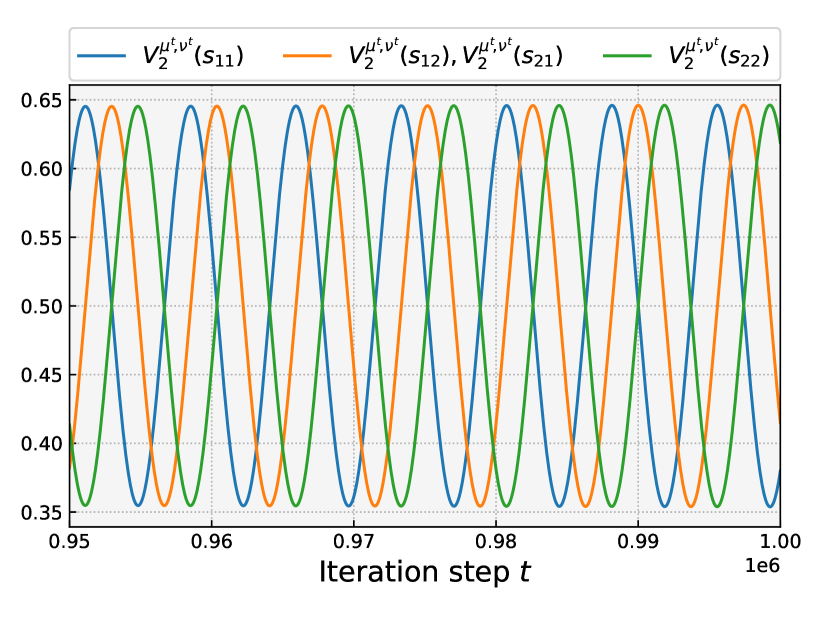
(a) Value functions at $h=2$

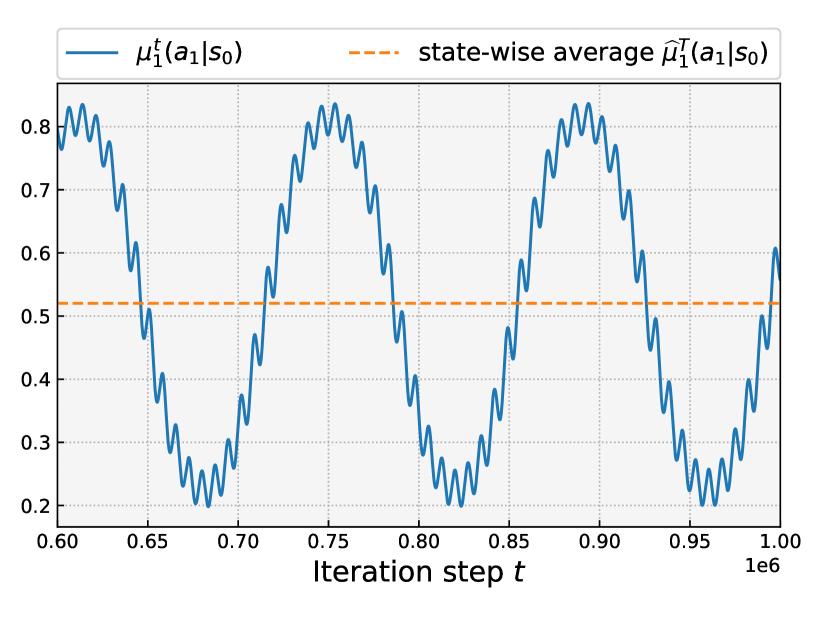
(b) Policy at $h=1$ ($\mu_{1}^{t}(a_{1}|s_{0})$)

Figure 2: Visualizations of the optimization trajectory of the INPG algorithm along a single run with $T=10^{6}$ and $\eta=1/\sqrt{T}$. (a) Value functions in the second layer $V^{\mu^{t},\nu^{t}}_{2}(s)$ for all four states $s\in{\left\{s_{11},s_{12},s_{21},s_{22}\right\}}$ over the last $5\times 10^{4}$ steps. (b) Policy in the first layer, i.e. $\mu_{1}^{t}(a_{1}|s_{0})$ over the last $4\times 10^{5}$ steps. The horizontal line plots the value of the final averaged policy $\widehat{\mu}_{1}^{T}(a_{1}|s_{0})$ (where the averaging is over the entire run $t\in[T]$).

H.2 Additional visualizations for the INPG algorithm

Figure 1 shows that the INPG algorithm (with $\eta=1/\sqrt{T}$) appears to converge much slower than $O(T^{-1/2})$ (which is the rate for FTRL with $\eta=1/\sqrt{T}$). Here we present some further understandings of this phenomenon by visualizing the optimization trajectories of the INPG algorithm.

Figure 2 shows the evolution of the value functions at $h=2$ over iteration step $t$, for the last $5\times 10^{4}$ steps. For all four states, the policy optimization is equivalent to Hedge on the matrix game with identity reward matrix 55, and thus exhibits an expected cyclic behavior and leads to the sinusoidal-like curves shown in Figure 2. However, due to the choice of our specific initialization $(\mu^{0},\nu^{0})$, the four curves behave like the same periodic curves with different “phases”.

Figure 2 shows the evolution of the policy at $h=1$ (specifically, $\mu_{1}^{t}(a_{1}|s_{0})$ which is the probability of the max-player taking action $a_{1}$) over $t$, for the last $4\times 10^{5}$ steps. (The result for the min-player is similar.) The curve also behaves periodically, and appears to be a superposition of two waves, one main waive with larger magnitude and period, and another oscillation with smaller magnitude and period. Qualitatively, the main wave is caused by the intrinsic cyclic behavior of learning with respect to the (fixed) reward at the $h=1$, while the oscillation is caused by the changing reward that is backed-up from $h=2$. Further, as the reward in the second layer has much higher magnitude than the first layer in this game, the oscillation has a non-negligible magnitude.

The horizontal line in Figure 2 plots the final output policy $\widehat{\mu}_{1}^{T}(a_{1}|s_{0})\approx 0.52$, which we recall is the average of $\mu_{1}^{t}(a_{1}|s_{0})$ over the entire run $t\in[T]$ (cf. Section 5). Note that the unique Nash equilibrium satisfies $\mu^{\star}_{1}(a_{1}|s_{0})=0.5$ (56), and the error $\widehat{\mu}_{1}^{T}(a_{1}|s_{0})-\mu_{1}^{\star}(a_{1}|s_{0})\approx 0.02$. We suspect that this may be an intrinsic bias caused by the aforementioned correlation between the two layers’ learning processes (in particular, the different “phases” of the second-layer’s learning over the four states), and may also be the cause of the slow convergence for INPG shown in Figure 1.

H.3 Additional theoretical justifications

INPG as an instantiation of Algorithm 1

Here we show why the instantiation of Algorithm 1 with $\beta_{t}=1$ and

$$\mu_{h}^{t}(a|s)\propto_{a}\mu_{h}^{t-1}(a|s)\exp\!{\left(\eta{\left[Q_{h}^{t-1}\nu_{h}^{t-1}\right]}(s)\right)},~{}~{}\nu_{h}^{t}(b|s)\propto_{b}\nu_{h}^{t-1}(b|s)\exp\!{\left(-\eta{\left[{\left(Q_{h}^{t-1}\right)}^{\!\top}\!\!\mu_{h}^{t-1}\right]}(s)\right)}.$$

considered in Section 5 is equivalent to the Independent Natural Policy Gradient (INPG) algorithm. Indeed, choosing $\beta_{t}=1$ in Algorithm 1 ensures that $Q_{h}^{t}=Q_{h}^{\mu^{t},\nu^{t}}$ (the true value function of $(\mu^{t},\nu^{t})$). Therefore, the above update is equivalent to

$$\mu_{h}^{t}(a|s)\!\propto_{a}\!\mu_{h}^{t-1}(a|s)\exp\!{\left(\eta{\left[Q_{h}^{\!\mu^{t\!-\!1}\!\!\!,\nu^{t\!-\!1}}\!\!\!\nu_{h}^{t\!-\!1}\right]}(s)\!\right)},~{}~{}\nu_{h}^{t}(b|s)\!\propto_{b}\!\nu_{h}^{t-1}(b|s)\exp\!{\left(\!\!-\eta{\left[{\left(Q_{h}^{\!\mu^{t\!-\!1}\!\!\!,\nu^{t\!-\!1}}\right)}^{\!\top}\!\!\mu_{h}^{t\!-\!1}\right]}(s)\!\right)}.$$

This is exactly an independent two-player version of the Natural Policy Gradient algorithm (e.g. [1]), where each player plays an NPG algorithm as if they are facing their own Markov Decision Process, with the opponent fixed.

NEGap-Layer-1 lower bounds ${\rm NEGap}$

Here we show NEGap-Layer-1$(\mu,\nu)\leq{\rm NEGap}(\mu,\nu)$ for any $(\mu,\nu)$. From the definition of $V_{h}^{\star}$ we have that

$$V_{h}^{\star}(s)=\inf_{\nu}V_{h}^{\dagger,\nu}(s)=\sup_{\mu}V_{h}^{\mu,\dagger},$$

$$\Longrightarrow~{}~{} V_{h}^{\mu,\dagger}\leq V_{h}^{\star}(s)\leq V_{h}^{\dagger,\nu}(s),~{}~{}\forall{\mu,\nu}.$$

Thus

$$Q_{h}^{\star}(s,a,b)={\left[r_{h}+\mathbb{P}_{h}V_{h+1}^{\star}\right]}(s,a,b)\leq{\left[r_{h}+\mathbb{P}_{h}V_{h+1}^{\dagger,\nu}\right]}(s,a,b)=Q_{h}^{\dagger,\nu}(s,a,b),$$

$$Q_{h}^{\star}(s,a,b)={\left[r_{h}+\mathbb{P}_{h}V_{h+1}^{\star}\right]}(s,a,b)\geq{\left[r_{h}+\mathbb{P}_{h}V_{h+1}^{\mu,\dagger}\right]}(s,a,b)=Q_{h}^{\mu,\dagger}(s,a,b)$$

$$\Longrightarrow \quad Q_{h}^{\mu,\dagger}(s,a,b)\leq Q_{h}^{\star}(s,a,b)\leq Q_{h}^{\dagger,\nu}(s,a,b).$$

Thus for our example

$$\textup{{\rm NEGap-Layer-1}}(\mu,\nu) =\max_{\mu_{1}^{\dagger}}{\left[(\mu_{1}^{\dagger})^{\top}Q^{\star}_{1}\nu_{1}\right]}(s_{0})-\min_{\nu_{1}^{\dagger}}{\left[\mu_{1}^{\top}Q^{\star}_{1}\nu_{1}^{\dagger}\right]}(s_{0})$$

$$\leq\max_{\mu_{1}^{\dagger}}{\left[(\mu_{1}^{\dagger})^{\top}Q^{\dagger,\nu}_{1}\nu_{1}\right]}(s_{0})-\min_{\nu_{1}^{\dagger}}{\left[\mu_{1}^{\top}Q^{\mu,\dagger}_{1}\nu_{1}^{\dagger}\right]}(s_{0})$$

$$=V_{1}^{\dagger,\nu}(s_{0})-V_{1}^{\mu,\dagger}(s_{0})={\rm NEGap}(\mu,\nu).$$

References

- Agarwal et al. [2021] A. Agarwal, S. M. Kakade, J. D. Lee, and G. Mahajan. On the theory of policy gradient methods: Optimality, approximation, and distribution shift. Journal of Machine Learning Research, 22(98):1–76, 2021.
- Bai and Jin [2020] Y. Bai and C. Jin. Provable self-play algorithms for competitive reinforcement learning. In International conference on machine learning, pages 551–560. PMLR, 2020.
- Bai et al. [2020] Y. Bai, C. Jin, and T. Yu. Near-optimal reinforcement learning with self-play. Advances in neural information processing systems, 33:2159–2170, 2020.
- Bard et al. [2020] N. Bard, J. N. Foerster, S. Chandar, N. Burch, M. Lanctot, H. F. Song, E. Parisotto, V. Dumoulin, S. Moitra, E. Hughes, et al. The hanabi challenge: A new frontier for ai research. Artificial Intelligence, 280:103216, 2020.
- Bhandari and Russo [2019] J. Bhandari and D. Russo. Global optimality guarantees for policy gradient methods. arXiv preprint arXiv:1906.01786, 2019.
- Brafman and Tennenholtz [2002] R. I. Brafman and M. Tennenholtz. R-max-a general polynomial time algorithm for near-optimal reinforcement learning. Journal of Machine Learning Research, 3(Oct):213–231, 2002.
- Cen et al. [2021a] S. Cen, C. Cheng, Y. Chen, Y. Wei, and Y. Chi. Fast global convergence of natural policy gradient methods with entropy regularization. Operations Research, 2021a.
- Cen et al. [2021b] S. Cen, Y. Wei, and Y. Chi. Fast policy extragradient methods for competitive games with entropy regularization. In M. Ranzato, A. Beygelzimer, Y. Dauphin, P. Liang, and J. W. Vaughan, editors, Advances in Neural Information Processing Systems, volume 34, pages 27952–27964. Curran Associates, Inc., 2021b.
- Chen and Peng [2020] X. Chen and B. Peng. Hedging in games: Faster convergence of external and swap regrets. Advances in Neural Information Processing Systems, 33:18990–18999, 2020.
- Chen et al. [2022] Z. Chen, D. Zhou, and Q. Gu. Almost optimal algorithms for two-player zero-sum linear mixture markov games. In International Conference on Algorithmic Learning Theory, pages 227–261. PMLR, 2022.
- Daskalakis et al. [2020] C. Daskalakis, D. J. Foster, and N. Golowich. Independent policy gradient methods for competitive reinforcement learning. Advances in neural information processing systems, 33:5527–5540, 2020.
- Daskalakis et al. [2021] C. Daskalakis, M. Fishelson, and N. Golowich. Near-optimal no-regret learning in general games. Advances in Neural Information Processing Systems, 34, 2021.
- de Witt et al. [2020] C. S. de Witt, T. Gupta, D. Makoviichuk, V. Makoviychuk, P. H. Torr, M. Sun, and S. Whiteson. Is independent learning all you need in the starcraft multi-agent challenge? arXiv preprint arXiv:2011.09533, 2020.
- Ding et al. [2020] D. Ding, K. Zhang, T. Basar, and M. Jovanovic. Natural policy gradient primal-dual method for constrained markov decision processes. Advances in Neural Information Processing Systems, 33:8378–8390, 2020.
- Ding et al. [2022] D. Ding, C.-Y. Wei, K. Zhang, and M. R. Jovanović. Independent policy gradient for large-scale markov potential games: Sharper rates, function approximation, and game-agnostic convergence. arXiv preprint arXiv:2202.04129, 2022.
- Filar and Vrieze [2012] J. Filar and K. Vrieze. Competitive Markov decision processes. Springer Science & Business Media, 2012.
- Golowich et al. [2020] N. Golowich, S. Pattathil, C. Daskalakis, and A. Ozdaglar. Last iterate is slower than averaged iterate in smooth convex-concave saddle point problems. In Conference on Learning Theory, pages 1758–1784. PMLR, 2020.
- Hansen et al. [2013] T. D. Hansen, P. B. Miltersen, and U. Zwick. Strategy iteration is strongly polynomial for 2-player turn-based stochastic games with a constant discount factor. Journal of the ACM (JACM), 60(1):1–16, 2013.
- Hu and Wellman [2003] J. Hu and M. P. Wellman. Nash q-learning for general-sum stochastic games. Journal of machine learning research, 4(Nov):1039–1069, 2003.
- Huang et al. [2021] B. Huang, J. D. Lee, Z. Wang, and Z. Yang. Towards general function approximation in zero-sum markov games. arXiv preprint arXiv:2107.14702, 2021.
- Jia et al. [2019] Z. Jia, L. F. Yang, and M. Wang. Feature-based q-learning for two-player stochastic games. arXiv preprint arXiv:1906.00423, 2019.
- Jin et al. [2018] C. Jin, Z. Allen-Zhu, S. Bubeck, and M. I. Jordan. Is q-learning provably efficient? Advances in neural information processing systems, 31, 2018.
- Jin et al. [2021a] C. Jin, Q. Liu, Y. Wang, and T. Yu. V-learning–a simple, efficient, decentralized algorithm for multiagent rl. arXiv preprint arXiv:2110.14555, 2021a.
- Jin et al. [2021b] C. Jin, Q. Liu, and T. Yu. The power of exploiter: Provable multi-agent rl in large state spaces. arXiv preprint arXiv:2106.03352, 2021b.
- Khodadadian et al. [2021] S. Khodadadian, P. R. Jhunjhunwala, S. M. Varma, and S. T. Maguluri. On the linear convergence of natural policy gradient algorithm. arXiv preprint arXiv:2105.01424, 2021.
- Lattimore and Szepesvári [2020] T. Lattimore and C. Szepesvári. Bandit algorithms. Cambridge University Press, 2020.
- Leonardos et al. [2021] S. Leonardos, W. Overman, I. Panageas, and G. Piliouras. Global convergence of multi-agent policy gradient in markov potential games. arXiv preprint arXiv:2106.01969, 2021.
- Littman [1994] M. L. Littman. Markov games as a framework for multi-agent reinforcement learning. In Machine learning proceedings 1994, pages 157–163. Elsevier, 1994.
- Littman et al. [2001] M. L. Littman et al. Friend-or-foe q-learning in general-sum games. In ICML, volume 1, pages 322–328, 2001.
- Liu et al. [2019] B. Liu, Q. Cai, Z. Yang, and Z. Wang. Neural trust region/proximal policy optimization attains globally optimal policy. Advances in neural information processing systems, 32, 2019.
- Liu et al. [2021] Q. Liu, T. Yu, Y. Bai, and C. Jin. A sharp analysis of model-based reinforcement learning with self-play. In International Conference on Machine Learning, pages 7001–7010. PMLR, 2021.
- Liu et al. [2022] Q. Liu, Y. Wang, and C. Jin. Learning markov games with adversarial opponents: Efficient algorithms and fundamental limits. arXiv preprint arXiv:2203.06803, 2022.
- Liu et al. [2020] Y. Liu, K. Zhang, T. Basar, and W. Yin. An improved analysis of (variance-reduced) policy gradient and natural policy gradient methods. Advances in Neural Information Processing Systems, 33:7624–7636, 2020.
- Mao and Başar [2021] W. Mao and T. Başar. Provably efficient reinforcement learning in decentralized general-sum markov games. arXiv preprint arXiv:2110.05682, 2021.
- Mei et al. [2020] J. Mei, C. Xiao, C. Szepesvari, and D. Schuurmans. On the global convergence rates of softmax policy gradient methods. In International Conference on Machine Learning, pages 6820–6829. PMLR, 2020.
- Mei et al. [2021] J. Mei, B. Dai, C. Xiao, C. Szepesvari, and D. Schuurmans. Understanding the effect of stochasticity in policy optimization. Advances in Neural Information Processing Systems, 34, 2021.
- Mordatch and Abbeel [2018] I. Mordatch and P. Abbeel. Emergence of grounded compositional language in multi-agent populations. In Proceedings of the AAAI Conference on Artificial Intelligence, volume 32, 2018.
- Peters and Schaal [2006] J. Peters and S. Schaal. Policy gradient methods for robotics. In 2006 IEEE/RSJ International Conference on Intelligent Robots and Systems, pages 2219–2225. IEEE, 2006.
- Rakhlin and Sridharan [2013] S. Rakhlin and K. Sridharan. Optimization, learning, and games with predictable sequences. Advances in Neural Information Processing Systems, 26, 2013.
- Rashid et al. [2018] T. Rashid, M. Samvelyan, C. Schroeder, G. Farquhar, J. Foerster, and S. Whiteson. Qmix: Monotonic value function factorisation for deep multi-agent reinforcement learning. In International Conference on Machine Learning, pages 4295–4304. PMLR, 2018.
- Samvelyan et al. [2019] M. Samvelyan, T. Rashid, C. S. De Witt, G. Farquhar, N. Nardelli, T. G. Rudner, C.-M. Hung, P. H. Torr, J. Foerster, and S. Whiteson. The starcraft multi-agent challenge. arXiv preprint arXiv:1902.04043, 2019.
- Schulman et al. [2015] J. Schulman, S. Levine, P. Abbeel, M. Jordan, and P. Moritz. Trust region policy optimization. In International conference on machine learning, pages 1889–1897. PMLR, 2015.
- Schulman et al. [2017] J. Schulman, F. Wolski, P. Dhariwal, A. Radford, and O. Klimov. Proximal policy optimization algorithms. arXiv preprint arXiv:1707.06347, 2017.
- Shani et al. [2020] L. Shani, Y. Efroni, and S. Mannor. Adaptive trust region policy optimization: Global convergence and faster rates for regularized mdps. In Proceedings of the AAAI Conference on Artificial Intelligence, volume 34, pages 5668–5675, 2020.
- Shapley [1953] L. S. Shapley. Stochastic games. Proceedings of the national academy of sciences, 39(10):1095–1100, 1953.
- Sidford et al. [2020] A. Sidford, M. Wang, L. Yang, and Y. Ye. Solving discounted stochastic two-player games with near-optimal time and sample complexity. In International Conference on Artificial Intelligence and Statistics, pages 2992–3002. PMLR, 2020.
- Song et al. [2021] Z. Song, S. Mei, and Y. Bai. When can we learn general-sum markov games with a large number of players sample-efficiently? arXiv preprint arXiv:2110.04184, 2021.
- Syrgkanis et al. [2015] V. Syrgkanis, A. Agarwal, H. Luo, and R. E. Schapire. Fast convergence of regularized learning in games. Advances in Neural Information Processing Systems, 28, 2015.
- Tian et al. [2021] Y. Tian, Y. Wang, T. Yu, and S. Sra. Online learning in unknown markov games. In International Conference on Machine Learning, pages 10279–10288. PMLR, 2021.
- Wei et al. [2017] C.-Y. Wei, Y.-T. Hong, and C.-J. Lu. Online reinforcement learning in stochastic games. In Advances in Neural Information Processing Systems, pages 4987–4997, 2017.
- Wei et al. [2021] C.-Y. Wei, C.-W. Lee, M. Zhang, and H. Luo. Last-iterate convergence of decentralized optimistic gradient descent/ascent in infinite-horizon competitive markov games. In Conference on Learning Theory, pages 4259–4299. PMLR, 2021.
- Xiao [2022] L. Xiao. On the convergence rates of policy gradient methods. arXiv preprint arXiv:2201.07443, 2022.
- Xie et al. [2020] Q. Xie, Y. Chen, Z. Wang, and Z. Yang. Learning zero-sum simultaneous-move markov games using function approximation and correlated equilibrium. arXiv preprint arXiv:2002.07066, 2020.
- Yu et al. [2021a] C. Yu, A. Velu, E. Vinitsky, Y. Wang, A. Bayen, and Y. Wu. The surprising effectiveness of ppo in cooperative, multi-agent games. arXiv preprint arXiv:2103.01955, 2021a.
- Yu et al. [2021b] T. Yu, Y. Tian, J. Zhang, and S. Sra. Provably efficient algorithms for multi-objective competitive rl. arXiv preprint arXiv:2102.03192, 2021b.
- Zhang et al. [2020] K. Zhang, S. M. Kakade, T. Başar, and L. F. Yang. Model-based multi-agent rl in zero-sum markov games with near-optimal sample complexity. arXiv preprint arXiv:2007.07461, 2020.
- Zhang et al. [2021a] K. Zhang, Z. Yang, and T. Başar. Multi-agent reinforcement learning: A selective overview of theories and algorithms. Handbook of Reinforcement Learning and Control, pages 321–384, 2021a.
- Zhang et al. [2021b] R. Zhang, Z. Ren, and N. Li. Gradient play in multi-agent markov stochastic games: Stationary points and convergence. CoRR, abs/2106.00198, 2021b.
- Zhang et al. [2022] R. Zhang, J. Mei, B. Dai, D. Schuurmans, and N. Li. On the effect of log-barrier regularization in decentralized softmax gradient play in multiagent systems, 2022.
- Zhao et al. [2021] Y. Zhao, Y. Tian, J. D. Lee, and S. S. Du. Provably efficient policy gradient methods for two-player zero-sum markov games. arXiv preprint arXiv:2102.08903, 2021.