Necessary and sufficient conditions to solve parabolic Anderson model with rough noise

Abstract.

We obtain necessary and sufficient conditions for the existence of $n$-th chaos of the solution to the parabolic Anderson model $\frac{\partial}{\partial t}u(t,x)=\frac{1}{2}\Delta u(t,x)+u(t,x)\dot{W}(t,x)$, where $\dot{W}(t,x)$ is a fractional Brownian field with temporal Hurst parameter $H_{0}\geq 1/2$ and spatial parameters $H$ $=(H_{1},\cdots,H_{d})$ $\in(0,1)^{d}$. When $d=1$, we extend the condition on the parameters under which the chaos expansion of the solution is convergent in the mean square sense, which is both sufficient and necessary under some circumstances.

1. Introduction

In this work, we study the solvability problem of the following stochastic heat equation on $\mathbb{R}^{d}$ ($d\geq 1$), also known as parabolic Anderson model (PAM):

$$\left\{\begin{aligned} &\frac{\partial}{\partial t}u(t,x)=\frac{1}{2}\Delta u(t,x)+u(t,x)\dot{W}(t,x)\,,~{}t>0\,;\\ &u(0,x)=u_{0}(x)\,,\end{aligned}\right.$$ (1.1)

where ${\Delta}=\sum_{i=1}^{d}\frac{\partial^{2}}{\partial x_{i}^{2}}$ is the Laplacian in $\mathbb{R}^{d}$, $\{W(t,x)\,,t\geq 0\,,x\in\mathbb{R}^{d}\}$ is a centered Gaussian field and $\dot{W}(t,x)=\frac{\partial^{1+d}}{\partial t\partial x_{1}\cdots\partial x_{d}}$. The covariance function of $\dot{W}(t,x)$ is given formally by

$$\text{Cov}(\dot{W}(t,x),\dot{W}(s,y))=\gamma_{0}(s-t)\gamma(x-y)\,.$$ (1.2)

In particular, we focus on the case

$$\gamma_{0}(t)=c_{H_{0}}|t|^{2H_{0}-2}\,,\quad\gamma(x)=\prod_{j=1}^{d}c_{H_{j},d}|x_{j}|^{2H_{j}-2}\,,$$ (1.3)

with the Hurst parameters $(H_{0},H_{1},\cdots,H_{d})$ satisfying $H_{0}\in[\frac{1}{2},1]$ and $H_{j}\in(0,1]$ $\forall j=1,\cdots,d$. The noise is called as space time white if $\gamma_{0}(\cdot)$ and $\gamma(\cdot)$ are Dirac delta functions. For the space time white noise, when the dimension $d=1$ and the initial condition is the Dirac delta function, the seminal paper [18] relates the equation (1.1) with the Kardar-Parisi-Zhang (KPZ) equation via the Hopf-Cole transformation $h(t,x)=\log(u(t,x))$ and develops the theory of regularity structures. In last decades, the parabolic Anderson model has received a great attention partly due to its connection to the KPZ equation. Recently, many sharp properties of solution to (1.1) have been obtained for general Gaussian noise, in particular, including the space time white noise setting when $d=1$. We refer [4, 11, 16, 26, 29, 31, 34] and references therein to the readers. However, the solvability problems for general Gaussian noise are still in the mists.

In current article, we interpret (1.1) in the Skorohod/Itô sense. The advantage to study (1.1) in this sense is that we can always write the solution candidate formally as its Itô-Wiener chaos expansion (see e.g. (2.14) below for more discussion):

$$u(t,x)=\sum_{n=0}^{\infty}u_{n}(t,x)=\sum_{n=0}^{\infty}\frac{1}{n!}I_{n}(f_{n}(\cdot,t,x))$$ (1.4)

and the (1.1) has a unique solution if and only if the above chaos expansion is convergent in $L^{2}(\Omega)$. In this case the solution $u(t,x)$ is given by the above sum. Thus, the solvability of (1.1) is reduced to two problems:

1. The first one is to evaluate $\mathbb{E}\left[u_{n}^{2}(t,x)\right]$, which can be reduced further to a complicate and singular multiple integrals.

2. The second one is to show the convergence of $\sum_{n=0}^{\infty}\mathbb{E}\left[u_{n}^{2}(t,x)\right]$, which requires sharp bounds of the $n$-th chaos $\mathbb{E}\left[u_{n}^{2}(t,x)\right]$ in terms of $n$.

As we see, the equation (1.1) depends only on the covariance structures ${\gamma}_{0}$ and ${\gamma}$. Usually, it is assumed that $\gamma_{0}(t)$ is locally integrable and $\gamma(x)$ is also locally integrable, which is represented by the Fourier transform of a positive measure $\mu$ on $\mathbb{R}^{d}$. Typically, one takes $\gamma_{0}(t)=\delta_{0}(t)$ or $\gamma_{0}(t)=c_{\alpha_{0}}|t|^{-\alpha_{0}}$ with $\alpha_{0}\in[0,1)$ and $c_{\alpha_{0}}>0$. As for the spatial covariance function $\gamma(x)$, three cases are commonly studied: (i) space white, i.e., $d=1$ and $\gamma(x)=\delta_{0}(x)$ or equivalently $\mu$ is the Lebesgue measure; (ii) Riesz potential, i.e., $\gamma(x)=c_{\alpha,d}|x|^{-\alpha}$ or equivalently $\mu(d\xi)=C_{\alpha,d}|\xi|^{-(d-\alpha)}\prod_{j=1}^{d}d\xi_{j}$ for some $0<\alpha<d$ and some positive constants $c_{\alpha,d},C_{\alpha,d}>0$; (iii) fractional, i.e., $\gamma(x)=\prod_{j=1}^{d}c_{\alpha_{j}}|x_{j}|^{-\alpha_{j}}$ or $\mu(d\xi)=\prod_{j=1}^{d}C_{\alpha_{j}}|\xi_{j}|^{-(1-\alpha_{j})}d\xi_{j}$ for some $0<\alpha_{j}<1$ and some positive constants $c_{\alpha_{j}},C_{\alpha_{j}}>0$. In the case $\gamma_{0}(\cdot)=\delta_{0}(\cdot)$ and ${\gamma}(x)$ is one of the above three cases, Dalang’s condition ([17]) implies that

$$\int_{\mathbb{R}^{d}}\frac{\mu(d\xi)}{1+|\xi|^{2}}<\infty\,\Leftrightarrow\,\begin{cases}\alpha<2&\text{Riesz kernel noise}\\ \sum_{j=1}^{d}{\alpha}_{j}<2&\text{fractional noise}\end{cases}$$ (1.5)

is necessary and sufficient for the existence of the solution to (1.1). When $\gamma_{0}(\cdot)$ is integrable, the Dalang’s condition (1.5) is also proved to be sufficient for the solvability in [24] in the general setting of Gaussian noise. Moreover, when ${\gamma}_{0}(t)=c_{\alpha}|t|^{-\alpha_{0}}$ and the spatial covariance $\gamma(\cdot)$ is given by the Riesz potential, the necessity of (1.5) has been obtained in [3]. Notice that in the fractional noise case, we usually take $\alpha_{j}=2-2H_{j}$. Thus, the Dalang’s condition $\sum_{j=1}^{d}{\alpha}_{j}<2$ becomes $\sum_{j=1}^{d}H_{j}>d-1$. As a comparison, we draw the attention to another random evolution model, the hyperbolic Anderson model (HAM) (i.e., we replace $\frac{\partial}{\partial t}$ by $\frac{\partial^{2}}{\partial t^{2}}$ in (1.1)). It is known that the Dalang’ condition (1.5) is a sufficient condition for the solvability of HAM. The readers are referred to [4] and references therein for details. During the preparation of this article, Chen, Deya, Song and Tindel in [14] obtain that

$$\int_{\mathbb{R}^{d}}\frac{1}{1+|\xi|^{3-\alpha_{0}}}\mu(d\xi)<\infty$$ (1.6)

is the necessary and sufficient condition for HAM to admit a unique Skorohod solution when $\alpha_{0}\in(0,1)$. Moreover, in the case of Riesz kernel or (regular) fractional noise, (1.6) is equivalent to $\alpha_{0}+\alpha<3$ or $\alpha_{0}+\sum_{j=1}^{d}\alpha_{j}<3$.

Recently, researchers are also interested in the case in which ${\gamma}(x)=\prod_{j=1}^{d}c_{\alpha_{j}}|x|^{-\alpha_{j}}$ and some of the ${\alpha}_{j}$’s may be greater than $1$. This means some of the Hurst parameters appeared in (1.3) are allowed to be less than $1/2$. Usually, the case when all the Hurst parameters are greater than $1/2$ is called regular. When at least one of the Hurst parameters is less than $1/2$, the corresponding noise is called rough. Rough case is more interesting and more challenging since the spatial covariance function is no longer locally integrable. Comparing to the regular case, although several significant progresses have been achieved, the solvability problem is still not completed. When $H_{0}=\frac{1}{2}$ (i.e., the noise is white in time) and $d=1$, the necessary and sufficient condition for the existence of solutions to PAM and HAM is known as $H_{1}>\frac{1}{4}$. The readers are referred to [5, 6, 22, 23, 30, 32] for further results. On the other hand when $H_{0}=1/2$ and $d>1$, it is known ([15]) that the number of Hurst parameters that are less than $1/2$ can be at most $1$ for (1.1) to be solvable.

The recent study on the rough noise is concentrated on the roughness of the Hurst parameters in space. There are very limited results on the case of rough in time, i.e., $H_{0}<1/2$. However, let us mention the work [27], where it is proved that all chaos of the solution candidate to (1.1) exists in $L^{2}(\Omega)$ when $H_{1}=1/2$ and $3/8<H_{0}<1/2$. Furthermore, if the noise is more smooth in spatial variable, then $H_{0}$ can be arbitrary (see e.g. [10, 25]).

When $H_{0}\geq 1/2$, and some of the spatial Hurst parameters are less than $1/2$ while others are greater than $1/2$, the solvability problem becomes much more complex and remains open although much more effort has been spent. Chen [12, 13] obtains some sufficient conditions on the parameters so that the solution is in $L^{2}(\Omega)$. Later on in the recent paper of Chen and Hu [15], these conditions are sharpened. More precisely, it is proved in [15] the following.

1. If $H_{0}=1/2$, namely if the noise is temporally white, then the necessary and sufficient conditions for (1.1) to be solvable (see e.g. [15, Theorem 1]) is that $H>1/4$ if $d=1$; $|H|:=\sum_{i=1}^{d}H_{i}>d-1$ and $H_{*}>\frac{3}{4}d_{*}-\frac{1}{2}$ if $d\geq 2$ ( the condition $H_{*}>\frac{3}{4}d_{*}-\frac{1}{2}$ is missing in [15, Theorem 1], see e.g. Proposition 4.5 in Section 4).

2. If $H_{0}>1/2$, then a sufficient condition for (1.1) to be solvable (see e.g. [15, Theorem 3 (i)]) is

   $$\begin{cases}H+H_{0}>\frac{3}{4}&\qquad\hbox{if $d=1$}\,,\\ |H|>d-1&\qquad\hbox{if $d\geq 2$}\,.\\ \end{cases}$$ (1.7)

3. If $H_{0}>1/2$, then a necessary condition for (1.1) to be solvable (see e.g. [15, Theorem 3 (ii)]) is

   $$\begin{cases}H+2H_{0}>\frac{5}{4}&\qquad\hbox{if $d=1$}\,,\\ |H|+2H_{0}>\frac{3d+2}{4}&\qquad\hbox{if $d\geq 2$}\,.\\ \end{cases}$$ (1.8)

This work ([15]) leaves an interesting open problem: In the case $H_{0}>1/2$, is (1.7) necessary or is (1.8) sufficient? Or the necessary and sufficient condition takes a completely different form? The present work is motivated by these problems and we shall provide a partial answer. More specifically, our first main result (Theorem 4.1) obtained in this paper is the necessary and sufficient conditions so that $\mathbb{E}\left[u_{n}^{2}(t,x)\right]<\infty$ for all $n$, where $u_{n}(t,x)$ is the $n$-chaos expansion of the solution candidate to (1.1). However, we still have difficulty to find the sharp dependence of $\mathbb{E}\left[u_{n}^{2}(t,x)\right]$ on $n$ to obtain the necessary and sufficient conditions for the summability of the chaos expansion of the solution. Focusing on $d=1$, our second main result (Theorem 5.1) shows that the first condition $H+2H_{0}>5/4$ in (1.8) is both necessary and sufficient for (1.1) to be solvable when $H_{0}<3/5$ or when $H>1/20$. This improves the condition $H+H_{0}>3/4$ in (1.7) which is deemed to be sharp.

To bound $\mathbb{E}\left[u_{n}^{2}(t,x)\right]$ we need to compute some very complicate integrals with both space variables $dx$ and time variables $dt$. To estimate the integral with respect to $dx$, we use the Fourier transforms to compute the corresponding integral with respect to $d\xi$. In order to obtain the necessary and sufficient condition, we need the sharp bounds of these integrals. It turns out that the bound on the evaluation of $d\xi$ obtained in previous works is not sharp when $H_{k}>3/4$. We improve these bounds in the case $H_{k}>3/4$ so that we have now the matching upper and lower bound, which is critical for the necessary and sufficient condition. This is done in Section 3 after some preparations in Section 2.

After obtaining the sharp bounds for the integration with respect to $d\xi$, we reduce the computation $\mathbb{E}\left[u_{n}^{2}(t,x)\right]$ to some multiple integrals with respect to time $t$. To estimate these multiple integrals, researchers use the Hardy-Littlewood-Sobolev inequality (see [27, 28] and references therein). It is also believed that this inequality is sharp for this problem and hence (1.7) is also necessary. However, contrary to the common belief, we shall show that (1.7) is not necessary and our results implicate that (1.8) may be sufficient.

To obtain better sufficient result we use, in addition to the Hardy-Littlewood-Sobolev inequality, the powerful Hölder-Young-Brascamp-Lieb inequality [9], improved by Avram and Taqqu [2] and by Bennett, Carbery, M Christ, and Tao ([7, 8]). We shall show how to verify the conditions so that these theorems can be applied. This is done in Section 4. In this section, we also give a more elementary proof of the sufficient condition by evaluating directly the concerning integrals. Since we still don’t have a sharp bound on the dependence of $\mathbb{E}\left[u_{n}^{2}(t,x)\right]$ on $n$, we keep these two alternative proofs for the sufficiency in hope that we may use one of these approaches to further obtain the right dependence of $\mathbb{E}\left[u_{n}^{2}(t,x)\right]$ on $n$. Let us also point out that to use the Hölder-Young-Brascamp-Lieb inequality for our purpose we may need to have a better understanding on the Brascamp-Lieb constant $C_{\text{BL}}$ associated with this inequality. More precisely, we believe that a much more patient analysis on the following Hölder-Young-Brascamp-Lieb inequality over the simplex $\mathbb{T}_{1}^{(n)}:=\{0\leq x_{1}<\cdots<x_{n}\leq 1\}$ is needed. Let $(c_{1},L_{1})\,\cdots\,,(c_{1},L_{m})$ be the Brasscamp-Lieb datum on $\mathbb{R}^{n}$, this is, each $c_{j}$ is a positive number and each $L_{j}:\mathbb{R}^{n}\to\mathbb{R}^{n_{j}}$ is a surjective linear mapping. Then

$$\int_{\mathbb{T}_{1}^{(n)}}\prod_{j=1}^{m}f_{j}(L_{j}x)^{c_{i}}dx\leq C_{\text{BL}}\prod_{j=1}^{m}\left(\int_{\mathbb{T}_{1}^{(n_{j})}}f_{j}(x)dx\right)^{c_{i}}$$ (1.9)

for all non-negative integrable functions $f_{j}:\mathbb{R}^{n_{j}}\to\mathbb{R}$.

In Section 5, the well accepted condition $H+H_{0}>\frac{3}{4}$ is enlarged to $H+2H_{0}>\frac{5}{4}$ by interpolating the results obtained by the Hardy-Littlewood-Sobolev inequality and that obtained by the Hölder-Young-Brascamp-Lieb inequality. It is also shown that $H+2H_{0}>\frac{5}{4}$ is the necessary and sufficient condition such that (1.1) has a unique solution on the regions $(H_{0},H)\in(\frac{1}{2},1)\times(\frac{1}{20},\frac{1}{2})$ or $(H_{0},H)\in(\frac{1}{2},\frac{3}{5})\times(0,\frac{1}{2})$.

In order to make the paper more readable, we delay some of the detailed computations to the appendix. In this appendix we also recall briefly the Hardy-Littlewood-Sobolev inequality and the Hölder-Young-Brascamp-Lieb inequality since they are the main tools in this work.

2. Preliminaries

In this section we first introduce some notations and facts that will be used in this paper. Let $\mathcal{C}_{0}^{\infty}(\mathbb{R}^{+}\times\mathbb{R}^{d})$ be the space of infinitely differentiable functions with compact support on $\mathbb{R}^{+}\times\mathbb{R}^{d}$. Since we shall work on the fractional Brownian noise whose Hurst parameters can be greater than $1/2$ for some coordinates and less than $1/2$ for other coordinates and since we are only concerned with the parabolic Anderson model, it is more convenient for us to introduce scalar product by using the Fourier transform with respect to spatial variables.

We denote the Fourier transform $\widehat{f}$ with respect to $d$ spatial variables $x_{1},\cdots,x_{d}$ as

$$\widehat{f}(\xi):=\mathcal{F}[f(x)]=\int_{\mathbb{R}^{d}}e^{-\iota\xi x}f(x)dx,\ \ \hbox{ where }\iota=\sqrt{-1}.$$

Let $H_{0}\in(1/2,1)$ and $H_{1},\cdots,H_{d}\in(0,1)$. Denote $\gamma_{0}(r)={\gamma}_{H_{0}}(r):=H_{0}(2H_{0}-1)|r|^{2H_{0}-2}\,,r\in\mathbb{R}$. We introduce a scalar product on $\mathcal{C}_{0}^{\infty}(\mathbb{R}^{+}\times\mathbb{R}^{d})$ as follows

$$\langle\varphi,\psi\rangle_{\mathfrak{H}}=\int_{\mathbb{R}_{+}^{2}\times\mathbb{R}^{d}}\hat{\varphi}(r,\bm{\xi})\overline{\hat{\psi}}(s,\bm{\xi})\prod_{k=1}^{d}|\xi_{k}|^{1-2H_{k}}\gamma_{0}(r-s)drdsd\bm{\xi},$$ (2.1)

where $\bm{\xi}:=(\xi_{1},\cdots,\xi_{d})$, $d\bm{\xi}:=d\xi_{1}\cdots d\xi_{d}$. Denote by $\mathfrak{H}$ the Hilbert space obtained from the completion of $\mathcal{C}_{0}^{\infty}(\mathbb{R}^{+}\times\mathbb{R}^{d})$ with respect to the scalar product $\langle\cdot,\cdot\rangle_{\mathfrak{H}}$.

The noise in the present paper is given by an isonormal Gaussian process $W=\{W(\varphi);\varphi\in\mathfrak{H}\}$ with covariance

$$\mathbb{E}[W(\varphi)W(\psi)]=\langle\varphi,\psi\rangle_{\mathfrak{H}}.$$

It is routine to prove that ${\bf 1}_{\left\{[0,t)\times\prod_{k=1}^{d}[0,x_{k}]\right\}}$ is in $\mathfrak{H}$ for any $t>0$, $x=(x_{1},\cdots,x_{d})\in\mathbb{R}^{d}$ (here we define ${\bf 1}_{[b,a]}=-{\bf 1}_{[a,b]}$ if $a<b$). Thus $W(t,x):=W({\bf 1}_{\{[0,t)\times\prod_{k=1}^{d}[0,x_{k}]\}})$. The Gaussian random field $\{W(t,x):t\geq 0,x\in\mathbb{R}^{d}\}$ have mean zero and covariance given by

$$\mathbb{E}[W(t,x)W(s,y)]= \ C_{H_{0},H}{\gamma}_{H_{0}}(t,s)\prod_{k=1}^{d}{\gamma}_{H_{k}}(x_{k},y_{k})\,,\quad s,t\geq 0\,,x,y\in\mathbb{R}^{d}\,,$$ (2.2)

where $C_{H_{0},H}$ is a constant depending on $H_{0},H=(H_{1},\cdots,H_{d})$. This constant $C_{H_{0},H}$ may be different from those in literature since we set the constant in (2.1) to be $1$.

Since the Gaussian field $W$ is not a martingale in time (because $H_{0}\not=1/2$), we cannot use the classical method of martingale measure to define stochastic integral. Thus, we shall use the chaos expansion to deal with our problem, and the most effective way for our purpose is then to introduce the stochastic integral via chaos multiple Itô-Wiener integrals (see [20, 21]).

Let $e_{1},\cdots,e_{n},\cdots\in\mathcal{C}_{0}^{\infty}(\mathbb{R}^{+}\times\mathbb{R}^{d})$ be an orthogonal basis of $\mathfrak{H}$. Then $\{\tilde{e}_{n}=W(e_{n}),n=1,2,\cdots\}$ are independent standard normal random variables. We denote by $\otimes$ the symmetric tensor product. The tensor product is then in $\mathfrak{H}^{\otimes n}$, where $n=n_{1}+\cdots+n_{k}$ and $e_{i_{1}},\cdots,e_{i_{k}}$ are all different. Let $H_{n}(x)=(-1)^{n}e^{\frac{x^{2}}{2}}\frac{d^{n}}{dx^{n}}(e^{-\frac{x^{2}}{2}})$ be the $n$-th Hermite polynomial. We define the multiple integral

$$I_{n}(e_{i_{1}}^{\otimes n_{1}}\otimes\cdots\otimes e_{i_{k}}^{\otimes n_{k}})=H_{n_{1}}(\tilde{e}_{i_{1}})\cdots H_{n_{k}}(\tilde{e}_{i_{k}})\,.$$

Any element in $\mathfrak{H}^{\otimes n}$ can be approximated by $f_{n}=\sum\limits_{0\leq n_{1},\cdots,n_{k}\leq n}a_{i_{1},\cdots,i_{k}}e_{i_{1}}^{\otimes n_{1}}\otimes\cdots\otimes e_{i_{k}}^{\otimes n_{k}}$, whose multiple Itô-Wiener integral is defined as

$$I_{n}(f_{n})= \sum_{0\leq n_{1},\cdots,n_{k}\leq n}a_{i_{1},\cdots,i_{k}}I_{n}(e_{i_{1}}^{\otimes n_{1}}\otimes\cdots\otimes e_{i_{k}}^{\otimes n_{k}})$$

$$= \sum_{0\leq n_{1},\cdots,n_{k}\leq n}a_{i_{1},\cdots,i_{k}}H_{n_{1}}(\tilde{e}_{i_{1}})\cdots H_{n_{k}}(\tilde{e}_{i_{k}})\,.$$

The Wiener chaos expansion theorem states that any random variable $F\in L^{2}(\Omega,\mathcal{F},\mathbb{P})$ admits a chaos expansion

$$F=\mathbb{E}[F]+\sum_{n=1}^{\infty}I_{n}(f_{n}),$$ (2.3)

where the series converges in $L^{2}(\Omega)$, and the elements $f_{n}\in{\mathfrak{H}}^{\otimes n}$ ( $n\geq 1$) are determined by $F$ and

$$\mathbb{E}|F|^{2}=(\mathbb{E}F)^{2}+\sum_{n=1}^{\infty}\mathbb{E}[|I_{n}(f_{n})|^{2}]=(\mathbb{E}F)^{2}+\sum_{n=1}^{\infty}n!\|{f}_{n}\|_{\mathfrak{H}^{\otimes n}}.$$ (2.4)

Let us recall that $\mathfrak{H}$ is the space of (maybe generalized) functions with $d+1$ variables whose Fourier transform with respect to spatial variables exist and its Hilbert norm associated with (2.1) is finite. The element in $\mathfrak{H}^{\otimes n}$ has formally the form $f(t_{1},x_{1},\cdots,t_{n},x_{n})$. It can be approximated by smooth functions from $\mathbb{R}_{+}^{n}\times\mathbb{R}^{nd}$ to $\mathbb{R}$ with compact support with respect to the norm $\mathfrak{H}^{\otimes n}$. We also write the multiple integral $I_{n}(f)$ as

$$I_{n}(f)=\int_{\mathbb{R}_{+}^{n}\times\mathbb{R}^{nd}}f(t_{1},x_{1},\cdots,t_{n},x_{n})W(dt_{1},dx_{1})\cdots W(dt_{n},dx_{n})\,.$$

The Fourier transform with respect to spatial variables of $f$ is given by

$$\hat{f}(t,\xi)=\hat{f}(t_{1},\xi_{1},\cdots,t_{n},\xi_{n})=\int_{\mathbb{R}^{nd}}f(t_{1},x_{1},\cdots,t_{n},x_{n})e^{-\iota\sum_{i=1}^{n}\xi_{i}x_{i}}dx_{1}\cdots dx_{n}\,,$$

where $\xi_{i}x_{i}=\sum_{k=1}^{d}\xi_{ik}x_{ik}$ is the Euclidean product of $\xi_{i}=(\xi_{i1},\cdots,\xi_{id})^{T}$, $x_{i}=(x_{i1},\cdots,x_{id})^{T}$ and $dx_{i}=dx_{i1}\cdots dx_{id}$. With these notations, we have

$$\|f\|_{\mathfrak{H}^{\otimes n}}^{2} = \int_{\mathbb{R}_{+}^{2n}\times\mathbb{R}^{nd}}\hat{f}(r_{1},\xi_{1},\cdots,r_{n},\xi_{n})\bar{\hat{f}}(s_{1},\xi_{1},\cdots,s_{n},\xi_{n})$$ (2.5)

$$\quad\prod_{i=1}^{n}\prod_{k=1}^{d}|\xi_{ik}|^{1-2H_{k}}\prod_{i=1}^{n}\gamma_{0}(r_{i}-s_{i})dr_{1}\cdots dr_{n}ds_{1}\cdots ds_{n}d\bm{\xi}\,.$$

Thus, any square integrable nonlinear functional of $W$ can be written as

$$F=\sum_{n=0}^{\infty}I_{n}(f)=\sum_{n=0}^{\infty}\int_{\mathbb{R}_{+}^{n}\times\mathbb{R}^{nd}}f_{n}(t_{1},x_{1},\cdots,t_{n},x_{n})W(dt_{1},dx_{1})\cdots W(dt_{n},dx_{n})\,,$$

for some sequence $f_{n}\in\mathfrak{H}^{\otimes n}$ and

$$\mathbb{E}[F^{2}] = \sum_{n=0}^{\infty}n!\int_{\mathbb{R}_{+}^{2n}\times\mathbb{R}^{nd}}\hat{f}(r_{1},\xi_{1},\cdots,r_{n},\xi_{n})\bar{\hat{f}}(s_{1},\xi_{1},\cdots,s_{n},\xi_{n})$$ (2.6)

$$\quad\prod_{i=1}^{n}\prod_{k=1}^{d}|\xi_{ik}|^{1-2H_{k}}\prod_{i=1}^{n}\gamma_{0}(r_{i}-s_{i})dr_{1}\cdots dr_{n}ds_{1}\cdots ds_{n}d\bm{\xi}\,.$$

Let $f:\mathbb{R}_{+}\times\mathbb{R}^{d}\times{\Omega}\to\mathbb{R}$ be a random field which is square integrable ($\mathbb{E}f^{2}(t,x)<\infty$). Then $f(t,x)$ admits a chaos expansion

$$f(t,x)=f_{0}(t,x)+\sum_{n=1}^{\infty}I_{n}(f_{n}(t,x))\,,$$

where $f_{n}(t,x)=f_{n}(t,x;t_{1},x_{1},\cdots,t_{n},x_{n})$ is an element in $\mathfrak{H}$ for any $t,x$. Let $\tilde{f_{n}}$ be the symmetrization of $f_{n}$:

$$\tilde{f_{n}}(t_{1},x_{1},\cdots,t_{n+1},x_{n+1})= \frac{1}{n+1}\sum_{i=1}^{n+1}f_{n}(t_{i},x_{i},t_{1},x_{1},\cdots,t_{i-1},x_{i-1},$$

$$\qquad\qquad\qquad t_{i+1},x_{i+1},\cdots,t_{n+1},x_{n+1})\,.$$ (2.7)

Definition 2.1.

We say $f(t,x)$ is integrable if for every $n\geq 0$, $\tilde{f_{n}}\in\mathfrak{H}^{\otimes(n+1)}$ and $\sum_{n=0}^{\infty}I_{n+1}(\tilde{f_{n}})$ is convergent in $L^{2}({\Omega})$. We define the stochastic integral of $f(t,x)$ as

$$\int_{\mathbb{R}_{+}\times\mathbb{R}^{d}}f(t,x)W(dt,dx)=\sum_{n=0}^{\infty}I_{n+1}(\tilde{f_{n}})\,.$$ (2.8)

We now give the concept of the strong (random field) solution to equation (1.1).

Definition 2.2.

A real-valued predictable stochastic process $u=\{u(t,x),t\geq 0,x\in\mathbb{R}^{d}\}$ is said to be a (global) random field solution (or mild solution) of (1.1) if for all $t\in[0,\infty)$ and $x\in\mathbb{R}^{d}$, $\{G_{t-\cdot}(x-\cdot)u(\cdot,\cdot)\}$ is integrable and the following equality holds almost surely,

$$u(t,x)=\int_{\mathbb{R}^{d}}G_{t}(x,y)u_{0}(y)dy+\int_{0}^{t}\int_{\mathbb{R}^{d}}G_{t-s}(x-y)u(s,y)W(ds,dy),$$ (2.9)

where $G_{t}(x)=(2\pi t)^{-d/2}\exp\left(-\frac{|x|^{2}}{2t}\right)$ is the heat kernel, the stochastic integral is understood in the sense of Definition 2.1. If equation (2.9) holds up to some time instant $t<t_{0}$ for some positive $t_{0}$, then we say that (1.1) has a local random field solution.

If $u(t,x)$ satisfies (2.9), then $u(s,y)$ has a similar representation. Substituting this expression into (2.9) we obtain a new equation for $u$. Carrying this procedure repeatedly, we see that if $u(t,x)$ is a strong solution of (1.1), then for each integer $N\geq 1$,

$$u(t,x)=\sum_{n=0}^{N}u_{n}(t,x)+\mathfrak{R}_{N}(t,x),$$ (2.10)

where

$$u_{n}(t,x)=\frac{1}{n!}I_{n}(f_{n}(t,x))$$ (2.11)

and $\mathfrak{R}_{N}(t,x)=I_{N+1}(g_{N}(t,x))$ with

$$f_{n}(t,x) := f_{n}(t,x,s_{1},x_{1},\dots,s_{n},x_{n})$$ (2.12)

is the symmetric extension with respect to $(s_{1},x_{1}),\cdots,(s_{n},x_{n})$ of

$$G_{t-s_{n}}(x-x_{n})G_{s_{n}-s_{n-1}}(x_{n}-x_{n-1})\cdots G_{s_{2}-s_{1}}(x_{2}-x_{1})G_{s_{1}}u_{0}(x_{1})\,,$$ (2.13)

where $0<s_{1}<s_{2}<\cdots<s_{n}<t$ and

$$g_{N}(t,x) = G_{t-s_{N+1}}(x-x_{N+1})G_{s_{N}-s_{N}}(x_{N+1}-x_{N})\cdots G_{s_{2}-s_{1}}(x_{2}-x_{1})u(s_{1},x_{1})\,.$$

It is easy to see that $\mathfrak{R}_{N}(t,x)$ is orthogonal to any multiple integral (of deterministic kernel) of order less than or equal to $N$. So if the solution $u(t,x)$ is in $L^{2}({\Omega})$, then it must admit the chaos expansion

$$u(t,x)=\sum_{n=0}^{\infty}u_{n}(t,x)=\sum_{n=0}^{\infty}\frac{1}{n!}I_{n}(f_{n}(t,x))\,,$$ (2.14)

where $f_{n}(t,x)$ is the symmetric extension of (2.13). On the other hand, if (2.14) is convergent in $L^{2}$, then it is easy to check that $\{G_{t-\cdot}(x-\cdot)u(\cdot,\cdot)\}$ is integrable and (2.9) holds so that $u(t,x)$ is a mild solution of (1.1). Thus, to study (1.1) we need to investigate the series (2.14).

Throughout the paper, $A\lesssim B$ ($A\gtrsim B$ and $A\simeq B$) means that there are strict positive universal constants $C_{1},C_{2}$ such that $A\leq C_{1}B$ ($A\geq C_{2}B$ and $C_{2}B\leq A\leq C_{1}B$).

3. Spatial Integration

To compute the $n$-th chaos $\mathbb{E}[u_{n}^{2}(t,x)]$, we shall use the Fourier transform for the Hilbert scalar product (2.1). In this section we are going to find sharp bounds of the integral with respect to $d\xi$ appeared in $\mathbb{E}[u_{n}^{2}(t,x)]$. To simply our notations, we introduce $\vec{\mathbf{s}}_{j}:=(s_{j},\cdots,s_{n})$ for all $1\leq j\leq n$ and $\vec{\mathbf{s}}:=\vec{\mathbf{s}}_{1}=(s_{1},\cdots,s_{n})$. Also, we use

$$\begin{cases}&d\vec{\mathbf{s}}_{j}:=ds_{j}ds_{j+1}\cdots ds_{n},\ \forall~{}1\leq j\leq n,\\ &d\vec{\mathbf{r}}_{j}:=dr_{j}dr_{j+1}\cdots dr_{n},\ \forall~{}1\leq j\leq n,\end{cases}$$ (3.1)

and $d\vec{\mathbf{s}}=d\vec{\mathbf{s}}_{1}$, $d\vec{\mathbf{r}}=d\vec{\mathbf{r}}_{1}$. Moreover, for any permutation $\sigma$ on $\{j,j+1,\cdots,n\}$ for $1\leq j\leq n$, we denote

$$\mathbb{T}_{t}(\vec{\mathbf{s}}_{j}\circ\sigma):=\{0=s_{0}<s_{\sigma(j)}<\cdots<s_{\sigma(n)}<s_{n+1}=t\}\,,$$ (3.2)

and $\mathbb{T}_{t}(\vec{\mathbf{s}}\circ\sigma):=\mathbb{T}_{t}(\vec{\mathbf{s}}_{1}\circ\sigma)$. If $\sigma$ is the natural permutation, then it is abbreviated as

$$\mathbb{T}_{t}(\vec{\mathbf{s}}_{j}\,):=\{0=s_{0}<s_{j}<\cdots<s_{n}<s_{n+1}=t\}\,,$$ (3.3)

and $\mathbb{T}_{t}(\vec{\mathbf{s}}):=\mathbb{T}_{t}(\vec{\mathbf{s}}_{1})$. The notations concerned with $\vec{\mathbf{r}}$ are defined similarly.

It is easy to see that Fourier transform of $f_{n}(t,x)$ with respect to spatial variables $x_{1},x_{2},\cdots,x_{n}$ in the symmetric extension of (2.13) is given by

$$\widehat{f}_{n}(t,x,s_{1},\xi_{1},\cdots,s_{n},\xi_{n})=\prod_{i=1}^{n}e^{-\frac{1}{2}(s_{{\sigma}(i+1)}-s_{{\sigma}(i)})|\xi_{{\sigma}(i)}+\cdots+\xi_{{\sigma}(1)}|^{2}}e^{-\iota x(\xi_{n}+\cdots+\xi_{1})}\,,$$ (3.4)

where $\vec{\mathbf{s}}=(s_{1},\cdots,s_{n})\in\mathbb{T}_{t}(\vec{\mathbf{s}}\circ\sigma)$.

Without loss of generality we assume $u_{0}(x)\equiv 1$ on $\mathbb{R}^{d}$ throughout the remaining part of this paper. For $n\geq 1$, $\vec{\mathbf{s}}\in\mathbb{T}_{t}(\vec{\mathbf{s}}\circ\varsigma)$ and $\vec{\mathbf{r}}\in\mathbb{T}_{t}(\vec{\mathbf{r}}\circ\sigma)$, where $\varsigma$ and ${\sigma}$ are two permutations of $\{1,2,\cdots,n\}$, by (2.1) and the definition of the tensor product norm we have that

$$\mathbb{E} \left[u_{n}^{2}(t,x)\right]$$

$$= \frac{1}{n!}\int_{{0<s_{1},\cdots,s_{n}<t\atop 0<r_{1},\cdots,r_{n}<t}}\int_{\mathbb{R}^{nd}}\prod_{i=1}^{n}e^{-\frac{1}{2}(s_{\varsigma(i+1)}-s_{\varsigma(i)})|\xi_{\varsigma(i)}+\cdots+\xi_{\varsigma(1)}|^{2}-\frac{1}{2}(r_{{\sigma}(i+1)}-r_{{\sigma}(i)})|\xi_{{\sigma}(i)}+\cdots+\xi_{{\sigma}(1)}|^{2}}$$

$$\qquad\qquad\qquad\qquad\qquad\qquad\qquad\prod_{i=1}^{n}\prod_{k=1}^{d}|\xi_{ik}|^{1-2H_{k}}d\xi_{1}\cdots d\xi_{n}\times\prod_{i=1}^{n}\gamma_{0}(s_{i}-r_{i})d\vec{\mathbf{s}}d\vec{\mathbf{r}}$$

$$= \int_{{0<s_{1}<\cdots<s_{n}<t\atop 0<r_{1},\cdots,r_{n}<t}}\int_{\mathbb{R}^{nd}}\prod_{i=1}^{n}e^{-\frac{1}{2}(s_{i+1}-s_{i})|\xi_{i}+\cdots+\xi_{1}|^{2}-\frac{1}{2}(r_{{\sigma}(i+1)}-r_{{\sigma}(i)})|\xi_{{\sigma}(i)}+\cdots+\xi_{{\sigma}(1)}|^{2}}$$

$$\qquad\qquad\qquad\qquad\qquad\qquad\qquad\prod_{i=1}^{n}\prod_{k=1}^{d}|\xi_{ik}|^{1-2H_{k}}d\xi_{1}\cdots d\xi_{n}\times\prod_{i=1}^{n}\gamma_{0}(s_{i}-r_{i})d\vec{\mathbf{s}}d\vec{\mathbf{r}}$$

$$= \int_{{0<s_{1}<\cdots<s_{n}<t\atop 0<r_{1},\cdots,r_{n}<t}}\prod_{k=1}^{d}h_{k,n}(\vec{\mathbf{s}},\vec{\mathbf{r}})\prod_{i=1}^{n}\gamma_{0}(s_{i}-r_{i})d\vec{\mathbf{s}}d\vec{\mathbf{r}}\,,$$ (3.5)

where $s_{n+1}=r_{n+1}:=t$. Moreover, when $\vec{\mathbf{s}}\in\mathbb{T}_{t}(\vec{\mathbf{s}})$ we define $h_{k,n}(\vec{\mathbf{s}})$ to be

$$h_{k,n}(\vec{\mathbf{s}}):= \int_{\mathbb{R}^{n}}\prod_{i=1}^{n}e^{-(s_{i+1}-s_{i})|\xi_{ik}+\cdots+\xi_{1k}|^{2}}\prod_{i=1}^{n}|\xi_{ik}|^{1-2H_{k}}d\xi_{1k}\cdots d\xi_{nk}$$

$$= \int_{\mathbb{R}^{n}}\prod_{i=1}^{n}e^{-(s_{i+1}-s_{i})|\eta_{i}|^{2}}\prod_{i=1}^{n}|\eta_{i}-\eta_{i-1}|^{1-2H_{k}}d\eta_{1}\cdots d\eta_{n}\,,$$ (3.6)

where we set $\eta_{0}:=0$ by convention and we make substitutions $\eta_{i}:=\xi_{ik}+\cdots+\xi_{1k}$. Then, by Hölder’s inequality we have

$$h_{k,n}(\vec{\mathbf{s}},\vec{\mathbf{r}}):= \int_{\mathbb{R}^{n}}\prod_{i=1}^{n}e^{-\frac{1}{2}(s_{i+1}-s_{i})|\xi_{ik}+\cdots+\xi_{1k}|^{2}-\frac{1}{2}(r_{{\sigma}(i+1)}-r_{{\sigma}(i)})|\xi_{{\sigma}(i),k}+\cdots+\xi_{{\sigma}(1),k}|^{2}}$$

$$\qquad\qquad\qquad\qquad\times\prod_{i=1}^{n}|\xi_{ik}|^{1-2H_{k}}d\xi_{1k}\cdots d\xi_{nk}$$ (3.7)

$$\leq h_{k,n}^{1/2}(\vec{\mathbf{s}})h_{k,n}^{1/2}(\vec{\mathbf{r}})\,.$$ (3.8)

In order to obtain a sharp bound for $h_{k,n}(\vec{\mathbf{s}})$, we shall write (3) as expectation of normal variables. Let $X_{0}=0$ and let $\{X_{1},\cdots,X_{n}\}$ be i.i.d standard Gaussian random variables. Set

$$w_{i}:=s_{i+1}-s_{i}\quad\hbox{for $1\leq i\leq n$}.$$ (3.9)

Then for $0<s_{1}<\cdots<s_{n}<t$, we have

$$h_{k,n} (\vec{\mathbf{s}})=c_{H_{k}}^{n}\left(\prod_{i=1}^{n}w_{i}^{-1/2}\right)\mathbb{E}\left[\prod_{i=1}^{n}\left|\frac{X_{i}}{\sqrt{w_{i}}}-\frac{X_{i-1}}{\sqrt{w_{i-1}}}\right|^{1-2H_{k}}\right]$$

$$=c_{H_{k}}^{n}\left(\prod_{i=1}^{n}w_{i}^{-1/2}\right)\left(\prod_{i=1}^{n}(w_{i}w_{i-1})^{H_{k}-1/2}\right)$$

$$\qquad\qquad\qquad\qquad\quad\times\mathbb{E}\left[\left|X_{1}\right|^{1-2H_{k}}\prod_{i=2}^{n}\left|\sqrt{w_{i-1}}X_{i}-\sqrt{w_{i}}X_{i-1}\right|^{1-2H_{k}}\right]$$

$$=c_{H_{k}}^{n}w_{n}^{H_{k}-1}\left(\prod_{i=1}^{n-1}w_{i}^{2H_{k}-3/2}\right)\left(\prod_{i=2}^{n}(w_{i}+w_{i-1})^{\frac{1}{2}-H_{k}}\right)$$

$$\qquad\times\mathbb{E}\left[\left|X_{1}\right|^{1-2H_{k}}\prod_{i=2}^{n}\left|\sqrt{\frac{w_{i-1}}{w_{i-1}+w_{i}}}X_{i}-\sqrt{\frac{w_{i}}{w_{i-1}+w_{i}}}X_{i-1}\right|^{1-2H_{k}}\right]\,.$$ (3.10)

Set

$${\lambda}_{1}=1\hbox{ and }\lambda_{i}:=\sqrt{\frac{w_{i-1}}{w_{i-1}+w_{i}}}\in(0,1)\ \ (i\geq 2).$$ (3.11)

Let us denote the expectation in (3.10) by $\mathfrak{I}_{k,n}$, namely, we denote

$$\mathfrak{I}_{k,n}:=\mathbb{E}\left[\left|X_{1}\right|^{1-2H_{k}}\prod_{i=2}^{n}\left|{\lambda_{i}}X_{i}-\sqrt{1-\lambda_{i}^{2}}X_{i-1}\right|^{1-2H_{k}}\right],$$ (3.12)

with the convention $\prod_{i=m}^{n}a_{i}:=1$ for $m>n$. To get a sharp bound for $h_{k,n}(\vec{\mathbf{s}})$, it suffices to get a sharp bound for $\mathfrak{I}_{k,n}$, which is given below.

Lemma 3.1.

We have the following upper bounds for $\mathfrak{I}_{k,n}$.

1. If $H_{k}<3/4$, then there is a positive constant $C_{H_{k}}$ such that

   $$\mathfrak{I}_{k,n}\leq C_{H_{k}}^{n}\,.$$ (3.13)

2. If $H_{k}\geq 3/4$, then for any ${\beta}_{k}\in(4H_{k}-3,2H_{k}-1)$, there is a positive constant $C_{{\beta}_{k}}$ such that

   $$\mathfrak{I}_{k,n}\leq C_{{\beta}_{k}}^{n}\prod_{i=2}^{n}{\lambda}_{i}^{-\beta_{k}}\,.$$ (3.14)

Proof.

We divide the proof into three steps, for the cases that $H_{k}$ is in $(0,1/2)$, $[1/2,3/4),\ [3/4,1)$ respectively.

Step 1: The case $0<H_{k}<\frac{1}{2}$. This case has been proven in [15]. More precisely,

$$\mathfrak{I}_{k,n} \leq C_{H_{k}}\mathbb{E}\left[\left|X_{1}\right|^{1-2H_{k}}\left(\prod_{i=2}^{n}\left(|X_{i}|\vee|X_{i-1}|\right)^{1-2H_{k}}\right)\right]$$ (3.15)

$$\leq C_{H_{k}}\mathbb{E}\left[\left|X_{1}\right|^{1-2H_{k}}\left(\prod_{i=2}^{n}\left(|X_{i}|+|X_{i-1}|\right)^{1-2H_{k}}\right)\right]$$

$$= C^{n}_{H_{k}}\,$$

for some $C_{H_{k}}>0$.

Step 2: The case $\frac{3}{4}\leq H_{k}<1$. To bound $\mathfrak{I}_{k,n}$ in this case, we shall use the following estimation for standard Gaussian random variable $X$  (see Lemma A.1 in [28] for details): for any $0<\alpha<1$, $\lambda>0$ and $b\in\mathbb{R}$, there is a constant $C_{\alpha}>0$ independent of $\lambda$ and $b$ so that

$$\mathbb{E}\left[|\lambda X+b|^{-\alpha}\right]\leq C_{\alpha}(\lambda\vee|b|)^{-\alpha}\simeq(\lambda+|b|)^{-\alpha}.$$ (3.16)

Now we set

$$\theta_{k}:=2H_{k}-1\,,\quad\zeta_{n}:=\prod_{i=1}^{n}\big{|}{\lambda_{i}}X_{i}-\sqrt{1-\lambda_{i}^{2}}\,X_{i-1}\big{|}^{-\theta_{k}}\,.$$ (3.17)

We also denote $\mathbb{E}^{Y}$ the expectation with respect to the random variable $Y$ while considering other random variables as constants. Thus, for any $1<p,q<+\infty$ satisfying $\frac{1}{p}+\frac{1}{q}=1$,

$$\mathfrak{I}_{k,n} =\mathbb{E}\left[\mathbb{E}^{X_{n}}\Big{[}\big{|}{\lambda_{n}}X_{n}-\sqrt{1-\lambda_{n}^{2}}\,X_{n-1}\big{|}^{-\theta_{k}}\zeta_{n-1}\Big{]}\right]$$

$$\leq C_{H_{k}}\mathbb{E}\left[\left(\sqrt{1-\lambda_{n}^{2}}\,|X_{n-1}|+\lambda_{n}\right)^{-\theta_{k}}\zeta_{n-1}\right]$$

$$\leq C_{H_{k}}{\lambda}_{n}^{-{\beta}_{k}}\mathbb{E}\bigg{\{}\mathbb{E}^{X_{n-1}}\bigg{[}\left(\sqrt{1-\lambda_{n}^{2}}\,|X_{n-1}|+\lambda_{n}\right)^{-\theta_{k}+{\beta}_{k}}$$

$$\qquad\qquad\qquad\qquad\qquad\big{|}{\lambda_{n-1}}X_{n-1}-\sqrt{1-\lambda_{n-1}^{2}}\,X_{n-2}\big{|}^{-\theta_{k}}\bigg{]}\zeta_{n-2}\bigg{\}}$$

$$\leq C_{H_{k}}{\lambda}_{n}^{-{\beta}_{k}}\mathbb{E}\Bigg{\{}\left[\mathbb{E}^{X_{n-1}}\left(\sqrt{1-\lambda_{n}^{2}}\,|X_{n-1}|+\lambda_{n}\right)^{-(\theta_{k}-{\beta}_{k})p}\right]^{1/p}$$

$$\qquad\qquad\quad\left[\mathbb{E}^{X_{n-1}}\big{|}{\lambda_{n-1}}X_{n-1}-\sqrt{1-\lambda_{n-1}^{2}}\,X_{n-2}\big{|}^{-\theta_{k}q}\right]^{1/q}\zeta_{n-2}\Bigg{\}}\,.$$ (3.18)

It is easy to see that under our assumption $4H_{k}-3<{\beta}_{k}<2H_{k}-1$, we have $2\theta_{k}-1<{\beta}_{k}<{\theta}_{k}$. This enables us to find $p$ and $q$ such that $0<(\theta_{k}-{\beta}_{k})p<1$ and $0<\theta_{k}q<1$ hold. Therefore,

$$\mathbb{E}^{X_{n-1}}\Big{(}\sqrt{1-\lambda_{n}^{2}} \,|X_{n-1}|+\lambda_{n}\Big{)}^{-(\theta_{k}-{\beta}_{k})p}$$

$$\leq C_{{\beta}_{k}}(\sqrt{1-\lambda_{n}^{2}}+\lambda_{n})^{-(\theta_{k}-{\beta}_{k})p}\leq C_{{\beta}_{k}}<\infty\,,$$ (3.19)

and

$$\mathbb{E}^{X_{n-1}}\big{|}{\lambda_{n-1}}X_{n-1} -\sqrt{1-\lambda_{n-1}^{2}}\,X_{n-2}\big{|}^{-\theta_{k}q}$$

$$\leq(\lambda_{n-1}+\sqrt{1-\lambda_{n-1}^{2}}\,|X_{n-2}|)^{-\theta_{k}q}\,.$$ (3.20)

Substituting (3) and (3) into (3.18) we have

$$\mathfrak{I}_{k,n}\leq C_{H_{k}}{\lambda}_{n}^{-{\beta}_{k}}\mathbb{E}\Bigg{\{}(\lambda_{n-1}+\sqrt{1-\lambda_{n-1}^{2}}\,|X_{n-2}|)^{-\theta_{k}}\varrho_{n-2}\Bigg{\}}\,.$$ (3.21)

Continuing this way we obtain that for any $2\theta_{k}-1<{\beta}_{k}<\theta_{k}$,

$$\mathfrak{I}_{k,n}\leq\ C_{{\beta}_{k}}^{n}\prod_{i=2}^{n}{\lambda}_{i}^{-{\beta}_{k}}.$$ (3.22)

Step 3: The case $\frac{1}{2}\leq H_{k}<\frac{3}{4}$. When $H_{k}=1/2$, it is easy to see that $\mathfrak{I}_{k,n}\equiv 1$. So we can assume $\frac{1}{2}<H_{k}<\frac{3}{4}$. The proof is similar to the case $H_{k}>\frac{3}{4}$ except that we take ${\beta}_{k}=0$ now and the proof is simpler. In fact, the Hölder inequality is valid since we can still find $p$ and $q$ such that $0<\theta_{k}p<1$ and $0<\theta_{k}q<1$ hold. In conclusion, we have

$$\mathfrak{I}_{k,n}\leq\ C_{H_{k}}^{n}\,.$$ (3.23)

This proves the lemma. ∎

To deal with the necessary condition in our main Theorem 4.1 in next section, we also need a lower bound for $\mathfrak{I}_{k,n}$. We can obtain the lower bound when $H_{k}<3/4$. However, we are still not clear about the lower bound of $\mathfrak{I}_{k,n}$ when $H_{k}\geq 3/4$ except when $n=2$. But this result is sufficient for our purpose.

Lemma 3.2.

We have the following lower bounds for $\mathfrak{I}_{k,n}$.

1. If $H_{k}<3/4$, then there is a positive constant $c_{H_{k}}$, independent of ${\lambda}_{i}$ ($1\leq i\leq n$) given by (3.11), such that

   $$\mathfrak{I}_{k,n}\geq c_{H_{k}}^{n}\,.$$ (3.24)

2. If $H_{k}\geq 3/4$, then there is a positive constant $c_{H_{k}}$, independent of ${\lambda}_{2}$ such that

   $$\mathfrak{I}_{k,2}\geq c_{H_{k}}{\lambda}_{2}^{-(4H_{k}-3)}\,,$$ (3.25)

   where ${\lambda}_{2}$ is defined by (3.11).

Proof.

First, we prove (1). Set $A_{n}:=\{X_{1}\leq 0,X_{2}\geq 0,\cdots,X_{2n-1}\leq 0,X_{2n}\geq 0\}$. When $0<H_{k}\leq\frac{1}{2}$, we have

$$\mathfrak{I}_{k,n}: =\mathbb{E}\left[\left|X_{1}\right|^{\theta_{k}}\prod_{i=2}^{n}\left|{\lambda_{i}}X_{i}-\sqrt{1-\lambda_{i}^{2}}X_{i-1}\right|^{-\theta_{k}}\right]$$

$$\geq\mathbb{E}\left[\left|X_{1}\right|^{\theta_{k}}\prod_{i=2}^{n}\left|{\lambda_{i}}X_{i}-\sqrt{1-\lambda_{i}^{2}}X_{i-1}\right|^{-\theta_{k}}\cdot{\bf 1}_{A_{n}}\right]$$

$$\geq c_{H_{k}}^{n}\ \mathbb{E}\left[|X_{1}|^{\theta_{k}}\left(\prod_{i=2}^{n}\left(|X_{i}|\wedge|X_{i-1}|\right)^{-\theta_{k}}\right)\cdot{\bf 1}_{A_{n}}\right]$$

$$\geq c_{H_{k}}^{n}\ \mathbb{E}\left[\left(|X_{1}|\wedge|X_{2}|\wedge\cdots\wedge|X_{n}|\right)^{-2\theta_{k}}\cdot{\bf 1}_{A_{n}}\right]$$

$$=c_{H_{k}}^{n}>0,$$

where $\theta_{k}$ is defined by (3.17).

When $\frac{1}{2}<H_{k}<\frac{3}{4}$, we see since $0\leq{\lambda}_{i}\leq 1$

$$\mathfrak{I}_{k,n}: =\mathbb{E}\left[\left|X_{1}\right|^{-\theta_{k}}\prod_{i=2}^{n}\left|{\lambda_{i}}X_{i}-\sqrt{1-\lambda_{i}^{2}}X_{i-1}\right|^{-\theta_{k}}\right]$$

$$\geq\mathbb{E}\left[|X_{1}|^{-\theta_{k}}\left(\prod_{i=2}^{n}\left(|X_{i}|+|X_{i-1}|\right)^{-\theta_{k}}\right)\right]$$

$$=c_{H_{k}}^{n}>0\,.$$

Now we prove (2). In this case $H_{k}>\frac{3}{4}$. We only need to consider the lower bound of $\mathfrak{I}_{k,2}$. We write

$$\mathfrak{I}_{k,2}({\lambda})=\mathbb{E}\left[|X_{1}|^{-\theta_{k}}\left|{\lambda}X_{2}-\sqrt{1-\lambda^{2}}X_{1}\right|^{-\theta_{k}}\right],\ \ \hbox{ ${\lambda}:={\lambda}_{2}\in(0,1)$,}$$

where $\theta_{k}:=2H_{k}-1$. It is obvious that $\mathfrak{I}_{k,2}({\lambda})$ is a continuous function of ${\lambda}\in(0,1]$. If ${\lambda}\to 1$, then $\mathfrak{I}_{k,2}({\lambda})\to\mathbb{E}\left[|X_{1}|^{-\theta_{k}}\left|X_{2}\right|^{-\theta_{k}}\right]>0$. We would like to see what is the behavior of this function when ${\lambda}$ is close to 0. For simplicity, we assume $0<{\lambda}<\frac{1}{2}.$   Then

$$\mathfrak{I}_{k,2} \simeq\mathbb{E}\left[|X_{1}|^{-\theta_{k}}\left|{\lambda}X_{2}-X_{1}\right|^{-\theta_{k}}\right]$$

$$=\frac{1}{\sqrt{2\pi}}\mathbb{E}\left[\int_{-\infty}^{\infty}|x_{1}|^{-{\theta}_{k}}|{\lambda}X_{2}-x_{1}|^{-{\theta}_{k}}e^{-\frac{x_{1}^{2}}{2}}dx_{1}\right]$$

$${\gtrsim}\ \mathbb{E}^{X_{2}}\left[\int_{0}^{1}|x_{1}|^{-{\theta}_{k}}|{\lambda}X_{2}-x_{1}|^{-{\theta}_{k}}dx_{1}\right]$$

$$=\mathbb{E}^{X_{2}}\left[|{\lambda}X_{2}|^{-2{\theta}_{k}+1}\cdot\int_{0}^{1/({\lambda}|X_{2}|)}|\tilde{x}_{1}|^{-{\theta}_{k}}|1-\tilde{x}_{1}|^{-{\theta}_{k}}d\tilde{x}_{1}\right]$$

$$\geq\mathbb{E}^{X_{2}}\left[|{\lambda}X_{2}|^{-2{\theta}_{k}+1}\cdot\int_{0}^{2/|X_{2}|}|\tilde{x}_{1}|^{-{\theta}_{k}}|1-\tilde{x}_{1}|^{-{\theta}_{k}}d\tilde{x}_{1}\right]$$

$${\gtrsim}\ \mathbb{E}^{X_{2}}\left[|{\lambda}X_{2}|^{-2{\theta}_{k}+1}\right],$$ (3.26)

where in the last equality we make change of variable $x_{1}\to{\lambda}|X_{2}|\tilde{x}_{1}$ and use the condition $H_{k}>\frac{3}{4}$. Moreover,

$$\mathbb{E}^{X_{2}}\left[|{\lambda}_{2}X_{2}|^{-2{\theta}_{k}+1}\right] \geq C{\lambda}^{-2{\theta}_{k}+1}\cdot\int_{0}^{1}x_{2}^{-2{\theta}_{k}+1}dx_{2}$$

$${\gtrsim}\ {\lambda}^{-2{\theta}_{k}+1}.$$ (3.27)

Substituting (3) into (3), we have

$$\mathfrak{I}_{k,2}{\gtrsim}\ {\lambda}^{-2{\theta}_{k}+1}={\lambda}^{3-4H_{k}}.$$ (3.28)

This completes the proof. ∎

From Lemma 3.1 and 3.2, we see that we need to handle the cases $H_{k}<3/4$ and $H_{k}\geq 3/4$ differently. We assume that there are $d_{*}$ index $k$’s such that $H_{k}<3/4$. Without loss of generality, we assume that the Hurst parameters are arranged so that $H_{k}<\frac{3}{4}$ for $k=1,2,\cdots,d_{*}$ and $H_{k}\geq\frac{3}{4}$ for $k=d_{*}+1,\cdots,d$. We also denote by $|H|$ the sum of all spatial Hurst parameters, by $H_{*}$ the sum of all Hurst parameters that are less than $3/4$ and by $H^{*}$ the sum of all Hurst parameters that are greater than or equal to $3/4$. Namely,

$$\begin{cases}H_{1},\cdots,H_{d_{*}}<3/4,\quad H_{d_{*}+1},\cdots,H_{d}\geq 3/4\,,\\ H_{*}:=H_{1}+\cdots+H_{d_{*}},\ \ \ H^{*}:=H_{d_{*}+1}+\cdots+H_{d}\,,\\ d^{*}=d-d_{*}\,,\quad|H|:=H_{1}+\cdots+H_{d}.\\ \end{cases}$$ (3.29)

Lemma 3.3.

Let $h_{n}(\vec{\mathbf{s}}):=\prod\limits_{k=1}^{d}h_{k,n}(\vec{\mathbf{s}})$, where $h_{k,n}(\vec{\mathbf{s}})\ (k=1,\cdots,d)$ are defined by (3). Take any  ${\beta}_{k}\in(4H_{k}-3,2H_{k}-1)$ for $k=d_{*}+1,\cdots,d$ and set

$${\beta}^{*}:={\beta}_{d_{*}+1}+\cdots+{\beta}_{d}\,.$$ (3.30)

Then we have the following estimations for $h_{n}(\vec{\mathbf{s}})$.

1. If $\frac{1}{2}d-|H|+\frac{1}{2}{\beta}^{*}>0,$ then

   $$h_{n}(\vec{\mathbf{s}})\leq C_{H}^{n}w_{n}^{|H|-d+{\alpha}_{n}}\sum_{\bm{{\alpha}}\in\mathcal{D}_{n}}\left(\prod_{i=1}^{n-1}w_{i}^{{\alpha}_{i}+2|H|-\frac{3}{2}d-\frac{1}{2}{\beta}^{*}}\right)\,,$$ (3.31)

   where $w_{i}$ $(1\leq i\leq n)$ are given by (3.9), $\mathcal{D}_{n}$ is the set of all indices $\bm{{\alpha}}=({\alpha}_{1},\cdots,{\alpha}_{n})$ such that

   $${\alpha}_{i}\in\left\{0,\frac{1}{2}d-|H|+\frac{1}{2}{\beta}^{*},d-2|H|+{\beta}^{*}\right\}\,,\quad{\alpha}_{i}+{\alpha}_{i+1}\not=0\,,\hbox{and}$$

   $$|\bm{{\alpha}}|=\sum_{i=1}^{n}{\alpha}_{i}=(n-1)(\frac{1}{2}d-|H|+\frac{1}{2}{\beta}^{*})\,.$$ (3.32)

   Moreover, if ${\alpha}_{i}=d-2|H|+{\beta}^{*}$, then both of ${\alpha}_{i-1}$ and ${\alpha}_{i+1}$ cannot be $\ d-2|H|+{\beta}^{*}$.

2. If $\frac{1}{2}d-|H|+\frac{1}{2}{\beta}^{*}\leq 0,$ then

   $$h_{n}(\vec{\mathbf{s}})\leq C_{H}^{n}\prod_{i=1}^{n}w_{i}^{|H|-d}.$$ (3.33)

Proof.

By Lemma 3.1, when $0<H_{k}<\frac{3}{4}$,

$$\mathfrak{I}_{k,n}\leq C^{n}_{H_{k}}\,.$$

Then, from (3.10) we obtain when $k\leq d_{*}$,

$$h_{k,n}(\vec{\mathbf{s}})\leq C_{H_{k}}^{n}w_{n}^{H_{k}-1}\left(\prod_{i=1}^{n-1}w_{i}^{2H_{k}-3/2}\right)\left(\prod_{i=2}^{n}(w_{i}+w_{i-1})^{\frac{1}{2}-H_{k}}\right).$$ (3.34)

When $\frac{3}{4}\leq H_{k}<1$, substitute (3.22) into (3.10), then for $d_{*}<k\leq d$,

$$h_{k,n}(\vec{\mathbf{s}}) \leq C_{H_{k}}^{n}w_{n}^{H_{k}-1}\left(\prod_{i=1}^{n-1}w_{i}^{2H_{k}-3/2}\right)\left(\prod_{i=2}^{n}(w_{i}+w_{i-1})^{\frac{1}{2}-H_{k}}\right)\times\left(\prod_{i=2}^{n}\lambda_{i}^{-{\beta}_{k}}\right).$$

Note that $\lambda_{i}=\sqrt{\frac{w_{i-1}}{w_{i-1}+w_{i}}}$ $(i\geq 2)$ which are defined in (3.11). Combining (3.34) and (3), we have

$$h_{n}(\vec{\mathbf{s}}) :=\prod_{k=1}^{d}{h_{k,n}(\vec{\mathbf{s}})}$$

$$\leq C_{H}^{n}\prod_{k=1}^{d}\left[w_{n}^{H_{k}-1}\left(\prod_{i=1}^{n-1}w_{i}^{2H_{k}-3/2}\right)\left(\prod_{i=2}^{n}(w_{i}+w_{i-1})^{\frac{1}{2}-H_{k}}\right)\right]\times\prod_{k=d_{*}+1}^{d}\prod_{i=2}^{n}{\lambda}_{i}^{-{\beta}_{k}}$$

$$\simeq C_{H}^{n}w_{n}^{|H|-d}\left(\prod_{i=1}^{n-1}w_{i}^{2|H|-\frac{3}{2}d-\frac{1}{2}{\beta}^{*}}\right)\left(\prod_{i=2}^{n}(w_{i}+w_{i-1})^{\frac{1}{2}d-|H|+\frac{1}{2}{\beta}^{*}}\right).$$ (3.36)

If $\frac{1}{2}d-|H|+\frac{1}{2}{\beta}^{*}>0$, from (4.7) it follows

$$h_{n}(\vec{\mathbf{s}})\leq C_{H}^{n}w_{n}^{|H|-d+{\alpha}_{n}}\sum_{\bm{{\alpha}}\in\mathcal{D}_{n}}\left(\prod_{i=1}^{n-1}w_{i}^{{\alpha}_{i}+2|H|-\frac{3}{2}d-\frac{1}{2}{\beta}^{*}}\right)\,,$$

where $\bm{{\alpha}}=({\alpha}_{1},\cdots,{\alpha}_{n})$ is in $\mathcal{D}_{n}$.

If $\frac{1}{2}d-|H|+\frac{1}{2}{\beta}^{*}\leq 0$, we can see by (4.7) that

$$h_{n}(\vec{\mathbf{s}}) \leq C_{H}^{n}w_{n}^{|H|-d}\left(\prod_{i=1}^{n-1}w_{i}^{2|H|-\frac{3}{2}d-\frac{1}{2}{\beta}^{*}}\right)\left(\prod_{i=2}^{n}w_{i-1}^{\frac{1}{2}d-|H|+\frac{1}{2}{\beta}^{*}}\right)$$

$$=C_{H}^{n}\prod_{i=1}^{n}w_{i}^{|H|-d}\,.$$

The lemma is then proved. ∎

Now we can compute $\mathbb{E}[|u_{n}(t,x)|^{2}]$ with $u_{n}(t,x)$ being defined by (2.11)-(2.13).

Lemma 3.4.

The $n$-th chaos $u_{n}(t,x)$ given by (2.11) can be bounded as follows. 
(1) If  $\frac{1}{2}d-|H|+\frac{1}{2}{\beta}^{*}>0$, then

$$\mathbb{E}[|u_{n}(t,x)|^{2}] {\lesssim}t^{n(|H|+2H_{0}-d)}n!\cdot\sum_{\bm{{\alpha}}\in\mathcal{D}_{n}}\int_{\mathbb{T}_{1}(\vec{\mathbf{s}})\times\mathbb{T}_{1}(\vec{\mathbf{r}})}(1-s_{n})^{-\rho_{n}}(1-r_{n})^{-\rho_{n}}$$

$$\qquad\times\prod_{i=1}^{n-1}|s_{i+1}-s_{i}|^{-\rho_{i}}\prod_{i=1}^{n-1}|r_{i+1}-r_{i}|^{-\rho_{i}}{\prod_{i=1}^{n}\gamma_{0}(s_{i}-r_{i})}d\vec{\mathbf{s}}d\vec{\mathbf{r}}\,,$$ (3.37)

with $\bm{{\alpha}}=({\alpha}_{1},\cdots,{\alpha}_{n})\in\mathcal{D}_{n}$ is given by (3.32) and

$$\begin{cases}&\rho_{i}=\frac{1}{2}(\frac{3}{2}d+\frac{1}{2}{\beta}^{*}-2|H|-{\alpha}_{i})\,,1\leq i\leq n-1,\\ &\rho_{n}=\frac{1}{2}(d-|H|-{\alpha}_{n})\,.\end{cases}$$ (3.38)

(2) If  $\frac{1}{2}d-|H|+\frac{1}{2}{\beta}^{*}\leq 0$, then

$$\mathbb{E}[|u_{n}(t,x)|^{2}] {\lesssim}t^{n(|H|+2H_{0}-d)}n!\cdot\sum_{\bm{{\alpha}}\in\mathcal{D}_{n}}\int_{\mathbb{T}_{1}(\vec{\mathbf{s}})\times\mathbb{T}_{1}(\vec{\mathbf{r}})}\prod_{i=1}^{n}|r_{i+1}-r_{i}|^{-\frac{1}{2}(d-|H|)}$$

$$\qquad\times\prod_{i=1}^{n}|s_{i+1}-s_{i}|^{-\frac{1}{2}(d-|H|)}{\prod_{i=1}^{n}\gamma_{0}(s_{i}-r_{i})}d\vec{\mathbf{s}}d\vec{\mathbf{r}}\,,$$ (3.39)

Proof.

By (3.5) and (3.8), we see that

$$\mathbb{E}\left[|u_{n}(t,x)|^{2}\right]{\lesssim} \int_{0<s_{1}<\cdots<s_{n}<t\atop 0<r_{1},\cdots,r_{n}<t}h_{n}^{1/2}(\vec{\mathbf{s}})h_{n}^{1/2}(\vec{\mathbf{r}})\prod_{i=1}^{n}\gamma_{0}(s_{i}-r_{i})d\vec{\mathbf{s}}d\vec{\mathbf{r}}\,,$$ (3.40)

Substituting the bound for $h_{n}$ obtained in Lemma 3.3 to the above inequality, we have

$$\mathbb{E}\left[u_{n}(t,x)^{2}\right]{\lesssim} \sum_{\bm{{\alpha}}\in\mathcal{D}_{n}}n!\int_{\mathbb{T}_{t}(\vec{\mathbf{s}})\times\mathbb{T}_{t}(\vec{\mathbf{r}})}(t-s_{n})^{\frac{1}{2}({\alpha}_{n}+|H|-d)}(t-r_{n})^{\frac{1}{2}({\alpha}_{n}+|H|-d)}$$

$$\qquad\qquad\times\prod_{i=1}^{n}\gamma_{0}(s_{i}-r_{i})\prod_{i=1}^{n-1}|s_{i+1}-s_{i}|^{\frac{1}{2}({\alpha}_{i}+2|H|-\frac{3}{2}d-\frac{1}{2}{\beta}^{*})}$$

$$\qquad\qquad\times\prod_{i=1}^{n-1}|r_{i+1}-r_{i}|^{\frac{1}{2}({\alpha}_{i}+2|H|-\frac{3}{2}d-\frac{1}{2}{\beta}^{*})}d\vec{\mathbf{s}}d\vec{\mathbf{r}}\,.$$ (3.41)

Now a changing of variables $s_{i}\to t\cdot s_{i}$ and $r_{i}\to t\cdot r_{i}$ $(1\leq i\leq n)$ yields (3.4). (3.4) can be proved similarly. ∎

Remark 3.5.

From equations (3.4) and (3.38) we see that we wish $\rho_{i}$ or ${\beta}^{*}$ to be as small as possible. Thus, we take $\beta_{k}=\left\{\left(4H_{k}-3\right)\vee 0\right\}+{\varepsilon}$ or ${\beta}^{*}=4H^{*}-3d^{*}+{\varepsilon}$ for any arbitrarily small ${\varepsilon}>0$. Since our conditions are in the form of strict inequality, we can let ${\varepsilon}=0$ in the following to simplify the presentation.

4. Necessary and sufficient condition

4.1. Main results

In this section, we shall show the necessary and sufficient conditions for $\mathbb{E}[u_{n}(t,x)^{2}]<+\infty$ for any fixed $n>1$, where $u_{n}(t,x)$ is the $n$-th Wiener-chaos expansion corresponding to $u(t,x).$ The definitions of $d_{*}$, $|H|$ and $H_{*}$ are given by (3.29).

Theorem 4.1.

Suppose $H_{0}\geq\frac{1}{2}$ and suppose $d_{*}$, $H_{*}$ and $|H|$ are given by (3.29). Let $u_{n}(t,x)$ be the $n$-th chaos candidate of the solution to (1.1), defined by (2.11)-(2.13). Then $\mathbb{E}[u_{n}(t,x)^{2}]<+\infty$ for $n>1$ if and only if the following conditions hold:

$$\begin{cases}&H_{*}>\frac{3}{4}d_{*}-1,\\ &|H|+2H_{0}>d,\\ &H_{*}+2H_{0}>\frac{3}{4}d_{*}+\frac{1}{2},\\ &|H|+2H_{*}+4H_{0}>d+\frac{3}{2}d_{*}.\end{cases}$$ (4.1)

When $d=1$, $H_{0}\geq\frac{1}{2}$ and $H=H_{1}<\frac{1}{2}$, the first condition in (4.1) is trivial. The second one and the last one are implied by the third one. Thus, we have

Corollary 4.2.

If $d=1$, $H_{0}\geq\frac{1}{2}$ and $0<H<\frac{1}{2}$, then the necessary and sufficient condition so that $\mathbb{E}[u_{n}(t,x)^{2}]<+\infty$ for $n>1$ becomes

$$H+2H_{0}>\frac{5}{4}\,.$$ (4.2)

If $H_{k}<3/4$ for all $k=1,\cdots,d$, we have $|H|=H_{*}$ and $d=d_{*}$. The conditions (4.1) can be slightly simplified to

Corollary 4.3.

If $H_{0}\geq\frac{1}{2}$ and $H_{k}<3/4$ for all $k=1,\cdots,d$, then the necessary and sufficient condition so that $\mathbb{E}[u_{n}(t,x)^{2}]<+\infty$ for $n>1$ becomes

$$\begin{cases}&H_{*}>\frac{3}{4}d-1,\\ &H_{*}+2H_{0}>(d\vee\frac{3d+2}{4}),\\ &3H_{*}+4H_{0}>\frac{5}{2}d.\end{cases}$$ (4.3)

Corollary 4.4.

Suppose $H_{0}\geq\frac{1}{2}$ and suppose the conditions in (4.1) hold.

1. If $H_{0}+H_{*}>\frac{3d_{*}}{4}$ and if $|H|>d-1$, then the solution is in $L^{p}(\Omega)$ for any $p\geq 1$. Moreover, there are two constants $C_{1,H}$ and $c_{2,H}$, independent of $p$, $t$ and $x$ such that

   $$\begin{split}\mathbb{E}\left[|u(t,x)|^{p}\right]\leq&C_{1,H}\exp\left[c_{2,H}p^{\frac{|H|-d+2}{|H|-d+1}}t^{\frac{|H|+2H_{0}-d}{|H|-d+1}}\right]\\ &\qquad\quad\qquad\quad\forall\ p\geq 1\,,\ t\geq 0\,,\ x\in\mathbb{R}^{d}\,.\end{split}$$ (4.4)

2. If $H_{0}+H_{*}>\frac{3d_{*}}{4}$ and if $|H|=d-1$, then there is a $t_{0}>0$ such that when $t<t_{0}$, $\mathbb{E}[u(t,x)^{2}]=\sum_{n=0}^{\infty}\mathbb{E}[u_{n}(t,x)^{2}]<+\infty$.

When $H_{0}=1/2$, the first and the forth conditions in (4.1) are implied by the second one and the third one. Therefore, combining Theorem 4.1 and Corollary 4.4, we have

Proposition 4.5.

Suppose $H_{0}=\frac{1}{2}$, namely, the noise is white in time. Then the necessary and sufficient condition for $\mathbb{E}[u(t,x)^{2}]<+\infty$ is

$$\begin{cases}&|H|>d-1\quad\hbox{and }\\ &H_{*}>\frac{3}{4}d_{*}-\frac{1}{2}.\end{cases}$$ (4.5)

This means that when the noise is white in time, the convergence of the Itô-Wiener chaos expansion is equivalent to the finiteness of each chaos.

4.2. Proof of Theorem 4.1: Sufficiency

Now we begin to prove the sufficiency in Theorem 4.1. Corollary 4.4 and Proposition 4.5 will be by-products of our proof. We only consider $H_{0}>1/2$. The case when $H_{0}=1/2$ can be proved in the same way. And condition (4.1) becomes (4.5) in this case. We shall show the proof for two cases: (I) $\frac{1}{2}d_{*}-H_{*}\leq d^{*}-H^{*}$ (or $\frac{3}{2}d_{*}-2H_{*}\leq d-|H|$ or $\frac{1}{2}d-|H|+\frac{1}{2}{\beta}^{*}\leq 0$) and (II) $\frac{1}{2}d_{*}-H_{*}>d^{*}-H^{*}$ (or $\frac{3}{2}d_{*}-2H_{*}>d-|H|$ or $\frac{1}{2}d-|H|+\frac{1}{2}{\beta}^{*}>0$).

The case $\frac{1}{2}d_{*}-H_{*}\leq d^{*}-H^{*}$. By (3.4), we have

$$\mathbb{E}[|u_{n}(t,x)|^{2}]{\lesssim} n!t^{n(|H|+2H_{0}-d)}\int_{\mathbb{T}_{1}(\vec{\mathbf{s}})\times\mathbb{T}_{1}(\vec{\mathbf{r}})}\prod_{i=1}^{n}(s_{i+1}-s_{i})^{\frac{|H|-d}{2}}$$

$$\qquad\qquad(r_{i+1}-r_{i})^{\frac{|H|-d}{2}}\cdot|s_{i}-r_{i}|^{2H_{0}-2}d\vec{\mathbf{s}}d\vec{\mathbf{r}}\,,$$ (4.6)

here in this case we use the convention $s_{n+1}=r_{n+1}=1$. Let $\tilde{h}_{n}(\vec{\mathbf{s}})$ be the symmetric extension of $\prod_{i=1}^{n}(s_{i+1}-s_{i})^{\frac{|H|-d}{2}}{\bf 1}_{\{0<s_{1}<\cdots<s_{n}<1\}}$ to $[0,1]^{n}$. The application of the Hardy-Littlewood-Soblev inequality (see Lemma A.2 in Appendix) yields

$$\mathbb{E}[|u_{n}(t,x)|^{2}]{\lesssim} (n!)^{-1}t^{n(|H|+2H_{0}-d)}\int_{[0,1]^{2n}}\tilde{h}_{n}(\vec{\mathbf{s}})\tilde{h}_{n}(\vec{\mathbf{r}})\cdot|s_{i}-r_{i}|^{2H_{0}-2}d\vec{\mathbf{s}}d\vec{\mathbf{r}}$$

$$= (n!)^{-1}t^{n(|H|+2H_{0}-d)}\left[\int_{[0,1]^{n}}\tilde{h}_{n}(\vec{\mathbf{s}})^{\frac{1}{H_{0}}}d\vec{\mathbf{s}}\right]^{2H_{0}}$$

$$\leq (n!)^{2H_{0}-1}t^{n(|H|+2H_{0}-d)}C_{H}^{n}\left(\int_{\mathbb{T}_{1}(\vec{\mathbf{s}})}\prod_{i=1}^{n}(s_{i+1}-s_{i})^{\frac{|H|-d}{2H_{0}}}d\vec{\mathbf{s}}\right)^{2H_{0}}$$

$$\approx (n!)^{2H_{0}-1}C_{H}^{n}t^{n(|H|+2H_{0}-d)}\left[\Gamma\left(\left(\frac{|H|-d}{2H_{0}}+1\right)n+1\right)\right]^{-2H_{0}}$$

$$= (n!)^{-(|H|-d+1)}C_{H}^{n}t^{n(|H|+2H_{0}-d)}$$ (4.7)

or

$$\|u_{n}(t,x)\|_{2}\leq C_{H}^{n}(n!)^{-\frac{|H|-d+1}{2}}t^{\frac{n(|H|+2H_{0}-d)}{2}}$$ (4.8)

under the condition

$$\frac{|H|-d}{2H_{0}}>-1\Leftrightarrow|H|+2H_{0}>d,$$

which is exactly the second inequality of (4.1). Moreover, we can see from (4.7) that $\mathbb{E}[|u_{n}(t,x)|^{2}]<+\infty$ under the above condition. Furthermore, by hypercontractivity inequality, we have

$$\|u_{n}(t,x)\|_{p}\leq p^{n/2}C_{H}^{n}(n!)^{-\frac{|H|-d+1}{2}}t^{\frac{n(|H|+2H_{0}-d)}{2}}\,.$$ (4.9)

Now, if

$$|H|>d-1\,,$$ (4.10)

then the chaos expansion of the solution is summable in $L^{p}(\Omega)$, and by the Mittag-Leffler theorem, we have

$$\mathbb{E}\left(\left|u(t,x)\right|^{p}\right)\leq \left(\sum_{n=0}^{\infty}\|u_{n}(t,x)\|_{p}\right)^{p}$$

$$\leq \left(\sum_{n=0}^{\infty}p^{n/2}C_{H}^{n}(n!)^{-\frac{|H|-d+1}{2}}t^{\frac{n(|H|+2H_{0}-d)}{2}}\right)^{p}$$

$$\approx C_{1,H}\exp\left[c_{2,H}p^{\frac{|H|-d+2}{|H|-d+1}}t^{\frac{|H|+2H_{0}-d}{|H|-d+1}}\right]\,.$$

It is interesting to note that the right hand side of (4.6) takes the minimum value when $H_{0}=1$, which is exactly equal to

$$n!t^{n(|H|+2-d)}\left[\int_{\mathbb{T}_{1}(\vec{\mathbf{s}})}\prod_{i=1}^{n}(s_{i+1}-s_{i})^{\frac{|H|-d}{2}}d\vec{\mathbf{s}}\right]^{2}$$

$$\qquad\approx t^{n(|H|+2-d)}(n!)^{1-2\left(1+\frac{|H|-d}{2}\right)}=(n!)^{-(|H|-d+1)}t^{n(|H|+2-d)}\,.$$ (4.11)

In terms of the exponent of $n!$, it is the same as our estimate (4.7). This means that our approach of using the Hardy-Littlewood-Sobolev inequality is “sharp” if we want that $u(t,x)$ is summable and $H_{0}$ seems play no role.

The case $\frac{1}{2}d_{*}-H_{*}>d^{*}-H^{*}$. This case is more complicated. From (3.4) in Lemma 3.4, it suffices for us to consider the following integral:

$$\mathcal{I}(\rho,\gamma):= \int_{\mathbb{T}_{1}(\vec{\mathbf{s}})\times\mathbb{T}_{1}(\vec{\mathbf{r}})}(1-s_{n})^{-\rho_{n}}(1-r_{n})^{-\rho_{n}}{\prod_{i=1}^{n}\gamma_{0}(s_{i}-r_{i})}$$ (4.12)

$$\qquad\qquad\times\prod_{i=1}^{n-1}|s_{i+1}-s_{i}|^{-\rho_{i}}\prod_{i=1}^{n-1}|r_{i+1}-r_{i}|^{-\rho_{i}}d\vec{\mathbf{s}}d\vec{\mathbf{r}}\,,$$

where $\rho_{i}$, $i=1,\cdots,n$ are given by (3.38). If we use the Hardy-Littlewood-Sobolev inequality as for (4.7), we obtain when $\rho_{i}<H_{0}$ for $i=1,\cdots,n$

$$\mathbb{E}[|u_{n}(t,x)|^{2}]{\lesssim} (n!)^{2H_{0}-1}t^{n(|H|+2H_{0}-d)}C_{H}^{n}\left(\int_{\mathbb{T}_{1}(\vec{\mathbf{s}})}\prod_{i=1}^{n}(s_{i+1}-s_{i})^{-\frac{\rho_{i}}{H_{0}}}d\vec{\mathbf{s}}\right)^{2H_{0}}$$

$$\approx (n!)^{2H_{0}-1}C_{H}^{n}t^{n(|H|+2H_{0}-d)}\left[\Gamma\left(\sum_{i=1}^{n}(1-\frac{\rho_{i}}{H_{0}})\right)\right]^{-2H_{0}}$$

$$= (n!)^{-(|H|-d+1)}C_{H}^{n}t^{n(|H|+2H_{0}-d)}\,.$$ (4.13)

From the definition of $\rho_{i}$’s, the condition $\rho_{i}<H_{0}$ for $i=1,\cdots,n$ is equivalent to

$$H_{0}+|H|>\frac{3}{4}d+\frac{\beta^{*}}{4}\quad\hbox{or}\quad H_{0}+H_{*}>\frac{3}{4}d_{*}\,.$$

This also proves Corollary 4.4 in this case.

Now we return to the problem of the finiteness of $\mathbb{E}\left[u_{n}^{2}(t,x)\right]$. It is obvious that $|H|\geq d-1$ is sufficient. But it is certainly not necessary since $H_{0}$ will play a role now. We would like to seek the necessary and sufficient conditions.

The right hand side of (3.4) is a multiple integral with some simple integrands. At first glance, we may think that the integrability problem of these kernels are simple. However, it seems this can be a complicate problem in analysis. There are some study about similar integrals (e.g. [33, 35, 36]). However, we cannot find results which are directly applicable. The difficulty is that the $\rho_{i}$ appeared in the integrand in (4.12) are different. To solve this integrability problem, our idea is to use both the Hardy-Littlewood-Sobolev inequality and the Hölder-Young-Brascamp-Lieb inequality obtained in [7], which we shall recall in Appendix A.

Take arbitrary $\bm{\alpha}:=(\alpha_{1},\cdots,\alpha_{n})\in\mathcal{D}_{n}$. Notice that ${\alpha}_{i}+{\alpha}_{i+1}\neq 0$. We divide our discussion on the integration $\mathcal{I}(\rho,\gamma)$ according to the following two cases.

$$\begin{cases}\hbox{\bf Case 1:}\qquad{\alpha}_{1}\neq 0\,,&\text{we use}\text{ the Hardy-Littlewood}\\ &\qquad\qquad\qquad\qquad\qquad\hbox{-Sobolev inequality}\,;\\ \hbox{\bf Case 2:}\qquad{\alpha}_{1}=0\,,{\alpha}_{2}\neq 0\,,&\text{we use }\text{ the H\"{o}lder-Young}\\ &\qquad\qquad\qquad\ \hbox{-Brascamp-Lieb inequality }\,.\end{cases}$$ (4.14)

Let us discuss the cases listed in (4.14) separately.

Case 1: When ${\alpha}_{1}\neq 0$, we integrate $s_{1}$ and $r_{1}$ in (4.12) first. This means we write

$$\mathcal{I}(\rho,\gamma):= \int_{\mathbb{T}_{1}(\vec{\mathbf{s}}_{2})\times\mathbb{T}_{1}(\vec{\mathbf{r}}_{2})}(1-s_{n})^{-\rho_{n}}(1-r_{n})^{-\rho_{n}}{\prod_{i=2}^{n}\gamma_{0}(s_{i}-r_{i})}$$ (4.15)

$$\times\prod_{i=2}^{n-1}|s_{i+1}-s_{i}|^{-\rho_{i}}\prod_{i=2}^{n-1}|r_{i+1}-r_{i}|^{-\rho_{i}}\mathcal{I}_{1}(s_{2},r_{2})d\vec{\mathbf{s}}_{2}d\vec{\mathbf{r}}_{2}\,,$$

where

$$\mathcal{I}_{1}(s_{2},r_{2}):=\int_{{0<s_{1}<s_{2}\atop 0<r_{1}<r_{2}}}\gamma_{0}(s_{1}-r_{1})|s_{2}-s_{1}|^{-\rho_{1}}|r_{2}-r_{1}|^{-\rho_{1}}dr_{1}ds_{1}\,.$$ (4.16)

Noticing that under the second inequality ($|H|+2H_{0}>d$) of (4.1), it holds

$$H_{0}-\rho_{1} =H_{0}-\frac{1}{2}\left[\frac{3}{2}d+\frac{1}{2}{\beta}^{*}-2|H|-{\alpha}_{1}\right]>0,$$ (4.17)

since ${\alpha}_{1}\in\left\{\frac{1}{2}d-|H|+\frac{1}{2}{\beta}^{*},d-2|H|+{\beta}^{*}\right\}$. Then an application of the Hardy-Littlewood-Sobolev inequality (Lemma A.2 in Appendix) yields

$$\mathcal{I}_{1}(s_{2},r_{2}){\lesssim} \left(\int_{0<s_{1}<s_{2}}|s_{2}-s_{1}|^{-\frac{\rho_{1}}{H_{0}}}ds_{1}\right)^{H_{0}}\left(\int_{0<r_{1}<r_{2}}|r_{2}-r_{1}|^{-\frac{\rho_{1}}{H_{0}}}dr_{1}\right)^{H_{0}}$$

$$= B\left(1,1-\frac{\rho_{1}}{H_{0}}\right)^{2H_{0}}s_{2}^{H_{0}-\rho_{1}}r_{2}^{H_{0}-\rho_{1}}{\lesssim}\ t^{2(H_{0}-\rho_{1})}\,,$$

where $B(x,y)=\frac{\Gamma(x)\Gamma(y)}{\Gamma(x+y)}$ is the Beta function.

Case 2: When ${\alpha}_{1}=0$, ${\alpha}_{2}\neq 0$, we integrate $s_{1},s_{2},r_{1},r_{2}$ in (4.12) first. Namely, we write now

$$\mathcal{I}(\rho,\gamma):= \int_{\mathbb{T}_{1}(\vec{\mathbf{s}}_{3})\times\mathbb{T}_{1}(\vec{\mathbf{r}}_{3})}(1-s_{n})^{-\rho_{n}}(1-r_{n})^{-\rho_{n}}{\prod_{i=3}^{n}\gamma_{0}(s_{i}-r_{i})}$$ (4.18)

$$\times\prod_{i=3}^{n-1}|s_{i+1}-s_{i}|^{-\rho_{i}}\prod_{i=3}^{n-1}|r_{i+1}-r_{i}|^{-\rho_{i}}\mathcal{I}_{2}(s_{3},r_{3})d\vec{\mathbf{s}}_{3}d\vec{\mathbf{r}}_{3}\,,$$

where

$$\mathcal{I}_{2}(s_{3},r_{3}):= \int_{{0<s_{1}<s_{2}<s_{3}\atop 0<r_{1}<r_{2}<r_{3}}}{\prod_{i=1}^{2}\gamma_{0}(s_{i}-r_{i})}|s_{3}-s_{2}|^{-\rho_{2}}|r_{3}-r_{2}|^{-\rho_{2}}$$

$$\qquad\qquad|s_{2}-s_{1}|^{-\rho_{1}}|r_{2}-r_{1}|^{-\rho_{1}}ds_{1}ds_{2}dr_{1}dr_{2}\,.$$ (4.19)

We claim that

$$\sup_{0\leq s_{3},r_{3}\leq t}\mathcal{I}_{2}(s_{3},r_{3})\leq C_{t}<+\infty\,.$$ (4.20)

This may be shown by some elementary computations. However, we shall prove it via the so called non-homogeneous Hölder-Young-Brascamp-Lieb inequality (see Theorem A.3 in Appendix). To use this theorem we let $\mathcal{H}:=\mathbb{R}^{4}$ and $\mathcal{H}_{j}:=\mathbb{R}$ for $j=1,\cdots,6$. Moreover, we introduce the following linear transformations $l_{j}:\mathcal{H}\to\mathcal{H}_{j}$

$$l_{1}(s_{1},s_{2},r_{1},r_{2})=r_{2}-r_{1}\,,~{}l_{3}(s_{1},s_{2},r_{1},r_{2})=r_{2}\,,~{}l_{5}(s_{1},s_{2},r_{1},r_{2})=s_{1}-r_{1}\,,$$

$$l_{2}(s_{1},s_{2},r_{1},r_{2})=s_{2}-s_{1}\,,~{}l_{4}(s_{1},s_{2},r_{1},r_{2})=s_{2}\,,~{}l_{6}(s_{1},s_{2},r_{1},r_{2})=s_{2}-r_{2}\,,$$

and the nonnegative functions $f_{j}:\mathcal{H}\to\mathbb{R}_{+}$

$$f_{1}(x)=|x|^{-\rho_{1}}{\bf 1}_{\{0<x<r_{3}\}}\,,~{}f_{3}(x)=|r_{3}-x|^{-\rho_{2}}{\bf 1}_{\{0<x<r_{3}\}}\,,~{}f_{5}(x)=|x|^{-\gamma}{\bf 1}_{\{|x|<1\}}\,,$$

$$f_{2}(x)=|x|^{-\rho_{1}}{\bf 1}_{\{0<x<s_{3}\}}\,,~{}f_{4}(x)=|s_{3}-x|^{-\rho_{2}}{\bf 1}_{\{0<x<s_{3}\}}\,,~{}f_{6}(x)=|x|^{-\gamma}{\bf 1}_{\{|x|<1\}}\,,$$

where

$$\begin{cases}&\rho_{1}=\frac{1}{2}\left(\frac{3}{2}d+\frac{1}{2}{\beta}^{*}-2|H|\right),\\ &\rho_{2}=\frac{1}{2}\left(\frac{3}{2}d+\frac{1}{2}{\beta}^{*}-2|H|-{\alpha}_{2}\right)\,,~{}\gamma=2-2H_{0}\,.\end{cases}$$

With these notations we can first bound $\mathcal{I}_{2}(s_{3},r_{3})$

$$\mathcal{I}_{2}(s_{3},r_{3})\leq \int_{{0<s_{1},s_{2}<1\atop 0<r_{1},r_{2}<1}}{\prod_{i=1}^{2}\gamma_{0}(s_{i}-r_{i})}|s_{3}-s_{2}|^{-\rho_{2}}{\bf 1}_{\{0<s_{2}<s_{3}\}}|r_{3}-r_{2}|^{-\rho_{2}}{\bf 1}_{\{0<r_{2}<r_{3}\}}$$

$$\qquad\times|s_{2}-s_{1}|^{-\rho_{1}}{\bf 1}_{\{0<s_{2}-s_{1}<s_{3}\}}|r_{2}-r_{1}|^{-\rho_{1}}{\bf 1}_{\{0<r_{2}-r_{1}<r_{3}\}}ds_{1}ds_{2}dr_{1}dr_{2}$$

$$=: \int_{[0,1]^{4}}\prod_{j=1}^{6}f_{j}(l_{j}(s_{1},s_{2},r_{1},r_{2}))ds_{1}ds_{2}dr_{1}dr_{2}=:\mathcal{J}(f_{1},\cdots,f_{6}).$$

Now the above integral is in a form that the Hölder-Young-Brascamp-Lieb theorem may apply. We want to show that under the condition (4.1) we can appropriately choose $p_{1},\cdots,p_{6}$ such that all the conditions of Theorem A.3 in the appendix are verified so that we can apply this Hölder-Young-Brascamp-Lieb theorem to obtain

$$\mathcal{I}_{2}(s_{3},r_{3})\leq\mathcal{J}(f_{1},\cdots,f_{6})\leq\prod_{j=1}^{6}\|f_{j}\|_{L^{p_{j}}(\mathbb{R})}\leq C<\infty\,.$$ (4.21)

To verify the conditions of Theorem A.3, we want to show that there exist $p_{1},\cdots,p_{6}$ so that

$$\begin{split}\hbox{$f_{j}\in L^{p_{j}}(\mathbb{R})$ and for every subspace $V\subseteq\mathcal{H}$:}\\ co\dim_{\mathcal{H}}(V)\geq\sum\limits_{j=1}^{6}\frac{1}{p_{j}}\cdot co\dim_{\mathcal{H}_{j}}(l_{j}(V))\,.\end{split}$$ (4.22)

Denote $z_{j}=p_{j}^{-1}\in(0,1]$ for $j=1,\cdots,6$. Take ${\beta}^{*}={\beta}_{d_{*}+1}+\cdots+{\beta}_{d}=4H^{*}-3d^{*}$ in Lemma 3.3. Then the integrability conditions $f_{j}\in L^{p_{j}}(\mathbb{R})$, $j=1,\cdots,6$ are equivalent to

$$\left\{\begin{split}&1\geq z_{1}\,,z_{2}>\rho_{1}=\frac{1}{2}(\frac{3}{2}d+\frac{1}{2}{\beta}^{*}-2|H|){=\frac{1}{2}\left(\frac{3}{2}d_{*}-2H_{*}\right)}\,,\\ &1\geq z_{3}\,,z_{4}>\rho_{2}=\frac{1}{2}(\frac{3}{2}d+\frac{1}{2}{\beta}^{*}-2|H|-{\alpha}_{2}){=\frac{1}{2}\left(\frac{3}{2}d_{*}-2H_{*}-{\alpha}_{2}\right)},\\ &1\geq z_{5}\,,z_{6}>\gamma=2-2H_{0}\,.\end{split}\right.$$ (4.23)

By the assumption $H_{0}>\frac{1}{2}$ we can choose $z_{5},z_{6}$ so that the third line in (4.23) holds true. We only need to explain that there are $z_{1}$ and $z_{2}$ such that the first line in (4.23) holds true since ${\alpha}_{2}>0$. Note that

$$\rho_{1}<1 \Leftrightarrow\frac{3}{2}d_{*}-2H_{*}<2\quad$$

$$\Leftrightarrow H_{*}>\frac{3}{4}d_{*}-1.$$

Therefore, the integrability conditions (4.23) are implied by the assumption $H_{0}>\frac{1}{2}$ and the first inequality of (4.1):

$$H_{*}>\frac{3}{4}d_{*}-1\,.$$ (4.24)

On the other hand, we need to verify the dimensional conditions in (4.22). For fixed co-dimension of $V$, our strategy is to select $V$ such that $co\dim_{\mathcal{H}_{j}}(l_{j}(V))=1$ as many as possible, i.e. $\dim_{\mathcal{H}_{j}}(l_{j}(V))=0$ as many as possible. It is not difficult to see that

$$\dim_{\mathcal{H}_{j}}(l_{j}(V))=0\ \hbox{if }\ V=\ker(l_{j}).$$

Therefore, we only need to take into account those $V$’s which are given by $\ker(l_{j})$ ($1\leq j\leq 6$) or their intersections. Thus, we shall select $J\subseteq\{1,\cdots,6\}$ such that $V=\cap_{j\in J}\ker(l_{j})$ and in this case

$$\dim_{\mathcal{H}}(V)= \dim(\cap_{j\in J}\ker(l_{j}))$$

$$= \dim(\mathcal{H})-\dim\left(span\{l_{j},j\in J\}\right)$$

$$= \dim(\mathcal{H})-{\rm rank}([l_{j}]_{j\in J})\,.$$ (4.25)

In the following, we shall discuss the cases $co\dim_{\mathcal{H}}(V)=4,3,2,1,0$. It is trivial to see the dimension condition (4.22) holds when $co\dim_{\mathcal{H}}(V)=0$. Therefore, we just have to verify (4.22) for $co\dim_{\mathcal{H}}(V)=4,3,2,1$ step by step. This is done in Lemma A.4 in Appendix under conditions (4.1).

This means that (4.21) is achieved under conditions (4.1) by using the non-homogeneous Hölder-Young-Brascamp-Lieb inequality.

To summarize we obtain that $\mathcal{I}(\rho,\gamma)$ defined by (4.12) can be bounded as

$$\mathcal{I}(\rho,\gamma)\leq B_{1}\cdot\int_{\mathbb{T}_{1}(\vec{\mathbf{s}}_{2})\times\mathbb{T}_{1}(\vec{\mathbf{r}}_{2})}(1-s_{n})^{-\rho_{n}}(1-r_{n})^{-\rho_{n}}{\prod_{i=2}^{n}\gamma_{0}(s_{i}-r_{i})}$$

$$\mathcal{I}(\rho,\gamma)\leq \qquad\times\prod_{i=2}^{n-1}|s_{i+1}-s_{i}|^{-\rho_{i}}\prod_{i=2}^{n-1}|r_{i+1}-r_{i}|^{-\rho_{i}}d\vec{\mathbf{s}}_{2}d\vec{\mathbf{r}}_{2}\quad\hbox{${\alpha}_{1}\neq 0$};$$

$$\mathcal{I}(\rho,\gamma)\leq$$ (4.26)

$$\mathcal{I}(\rho,\gamma)\leq C\cdot\int_{\mathbb{T}_{1}(\vec{\mathbf{s}}_{3})\times\mathbb{T}_{1}(\vec{\mathbf{r}}_{3})}(1-s_{n})^{-\rho_{n}}(1-r_{n})^{-\rho_{n}}{\prod_{i=3}^{n}\gamma_{0}(s_{i}-r_{i})}$$

$$\mathcal{I}(\rho,\gamma)\leq \qquad\times\prod_{i=3}^{n-1}|s_{i+1}-s_{i}|^{-\rho_{i}}\prod_{i=3}^{n-1}|r_{i+1}-r_{i}|^{-\rho_{i}}d\vec{\mathbf{s}}_{3}d\vec{\mathbf{r}}_{3}\,,\quad\hbox{${\alpha}_{1}=0\,,{\alpha}_{2}\neq 0$}.$$

$$\mathcal{I}(\rho,\gamma)\leq$$ (4.27)

where $B_{1}:=B\left(1,1-\frac{\rho_{1}}{H_{0}}\right)^{2H_{0}}$. The remaining integration has the same form as the original one but with strictly less multiplicity. We can then use the same argument as above to prove

$$\mathcal{I}(\rho,\gamma)\leq C^{n}<\infty.$$

Thus, we have

$$\mathbb{E}[|u_{n}(t,x)|^{2}]\leq C^{n}\cdot n!\cdot t^{n(|H|+2H_{0}-d)}<\infty\,.$$ (4.28)

As a result, we have proven (4.28) under the conditions (4.1) and we finish the proof of sufficiency in Theorem 4.1.

4.3. Sufficient condition of Theorem 4.1: An alternative proof

In this subsection, we give another proof of the sufficient condition using some elementary computations in the Appendix A.

As explained in the previous section, we need to show $\mathcal{I}_{1}(s_{2},r_{2})$ defined by (4.16) is bounded under the condition ${\alpha}_{1}\not=0$ and $\mathcal{I}_{2}(s_{3},r_{3})$ defined by (4.2) is bounded under the condition ${\alpha}_{1}=0$ but ${\alpha}_{2}\not=0$. Recall that

$$\begin{split}\rho_{i}=&\frac{1}{2}(\frac{3}{2}d+\frac{1}{2}{\beta}^{*}-2|H|-{\alpha}_{i})\\ =&\begin{cases}\frac{3}{4}d_{*}-H_{*},&\qquad\hbox{if ${\alpha}_{i}=0$}\\ \frac{d-|H|}{2},&\qquad\hbox{if ${\alpha}_{i}=\frac{1}{2}d-|H|+\frac{1}{2}{\beta}^{*}$}.\\ \end{cases}\end{split}$$

Case 1: ${\alpha}_{1}\not=0$. In this case, we apply Lemma A.7 to $\mathcal{I}_{1}(s_{2},r_{2})$ with

$$\mathfrak{{\beta}} = 0\,,\quad{\gamma}=2-2H_{0}\,,\quad a=b=0\,,\quad A=s_{2}\,,\quad B=r_{2}\,,$$

$${\alpha} = \rho_{1}=\frac{1}{2}(\frac{3}{2}d+\frac{1}{2}{\beta}^{*}-2|H|-{\alpha}_{1})\,,$$

and ${\alpha}_{1}\in\left\{\frac{1}{2}d-|H|+\frac{1}{2}{\beta}^{*},d-2|H|+{\beta}^{*}\right\}$. In order to use this lemma, we should require the following condition

$${\gamma}<2-{\alpha}\Leftrightarrow H_{*}+2H_{0}>\frac{3}{4}d_{*},$$

which is implied by the third inequality of (4.1). Then,

$$\mathcal{I}_{1}(s_{2},r_{2})\lesssim s_{2}^{1-\rho_{1}-\frac{{\gamma}}{2}}r_{2}^{1-\rho_{1}-\frac{{\gamma}}{2}}+s_{2}^{1-\rho_{1}-q_{2}}r_{2}^{1-\rho_{1}-q_{2}}|r_{2}-s_{2}|^{-{\gamma}+2q_{2}}.$$ (4.29)

The right hand side of (4.29) is bounded if

$$\begin{cases}1-\rho_{1}-\frac{{\gamma}}{2}>0\,;\\ -{\gamma}+2q_{2}\geq 0\,,\end{cases}$$ (4.30)

for some $q_{2}\in(0,(1-\rho_{1})\wedge\frac{{\gamma}}{2}]$. Since $\alpha_{1}\not=0$, it follows that $\rho_{1}\leq\frac{1}{2}(d-|H|)$. The first condition of (4.30) is then equivalent to $|H|+2H_{0}>d$, which is the second inequality in (4.1). Since the first condition of (4.30) holds true, we have $\frac{\gamma}{2}<1-\rho_{1}$. Then we can take $q_{2}=\frac{\gamma}{2}$ and we see easily hat the second condition of (4.30) is true.

Case 2: ${\alpha}_{1}=0$ and ${\alpha}_{2}\not=0$. We shall use Lemma A.7 to bound $\mathcal{I}_{2}(s_{3},r_{3})$ given by (4.2). Notice that in this case we should also integrate $\mathcal{I}_{1}(s_{2},r_{2})$ first to obtain (4.29). But in this case since ${\alpha}_{1}=0$, it follows

$$\rho_{1}=\frac{1}{2}(\frac{3}{2}d+\frac{1}{2}{\beta}^{*}-2|H|)=\frac{1}{2}\left(\frac{3}{2}d_{*}-2H_{*}\right).$$

In order to use Lemma A.7, we need $\rho_{1}<1$. This is equivalent to

$$H_{*}>\frac{3}{4}d_{*}-1$$ (4.31)

which is the first inequality in (4.1). Under this condition we can estimate $\mathcal{I}_{1}(s_{2},r_{2})$ as (4.29).

If $\frac{{\gamma}}{2}\leq 1-\rho_{1}$, then we can choose $q_{2}=\frac{{\gamma}}{2}$ and $\mathcal{I}_{1}(s_{2},r_{2})$ is also bounded. Hence, in this case we may proceed as in the case ${\alpha}_{1}\not=0$.

If $\frac{{\gamma}}{2}>1-\rho_{1}$, namely,

$$H_{0}+H_{*}<\frac{3}{4}d_{*}\,,$$ (4.32)

then this case we choose $q_{2}=1-\rho_{1}$ and we have to consider the integral $\mathcal{I}_{2}(s_{3},r_{3})$ given by (4.2). We integrate $s_{1}$ and $r_{1}$ first. By (4.29), we have

$$\mathcal{I}_{2}(s_{3},r_{3})\leq \int_{{0<s_{2}<s_{3}\atop 0<r_{2}<r_{3}}}|s_{3}-s_{2}|^{-\rho_{2}}|r_{3}-r_{2}|^{-\rho_{2}}(s_{2}r_{2})^{1-\rho_{1}-\frac{{\gamma}}{2}}|s_{2}-r_{2}|^{-{\gamma}}ds_{2}dr_{2}$$

$$+\int_{{0<s_{2}<s_{3}\atop 0<r_{2}<r_{3}}}|s_{3}-s_{2}|^{-\rho_{2}}|r_{3}-r_{2}|^{-\rho_{2}}|s_{2}-r_{2}|^{-2{\gamma}+2-2\rho_{1}}ds_{2}dr_{2}$$

$$=:\mathcal{I}_{2,1}(s_{3},r_{3})+\mathcal{I}_{2,2}(s_{3},r_{3})\,,$$ (4.33)

where ${\gamma}=2-2H_{0}$,

$$\rho_{2}=\frac{1}{2}(\frac{3}{2}d+\frac{1}{2}{\beta}^{*}-2|H|-{\alpha}_{2})\quad\hbox{and}\quad{\alpha}_{2}\in\left\{\frac{1}{2}d-|H|+\frac{1}{2}{\beta}^{*},d-2|H|+{\beta}^{*}\right\}\,.$$

To use Lemma A.7 for $\mathcal{I}_{2,1}(s_{3},r_{3})$, we need

$${1-\rho_{1}-\frac{{\gamma}}{2}}>-1\Leftrightarrow H_{*}+H_{0}>\frac{3}{4}d_{*}-1\,,$$

which is implied by the first condition of (4.1). Similarly, for the term $\mathcal{I}_{2,2}(s_{3},r_{3})$, we need

$$-2{\gamma}+2-2\rho_{1}>-1\,.$$

This condition is equivalent to

$$2H_{0}+H_{*}>\frac{3}{4}d_{*}+\frac{1}{2}\,,$$ (4.34)

which is the third condition in (4.1).

Now we apply Lemma A.7 to $\mathcal{I}_{2,1}(s_{3},r_{3})$ with

$${\alpha}=\rho_{2},\ {\beta}=-(1-\rho_{1}-\frac{{\gamma}}{2}),\ a=b=0,\ A=s_{3}\hbox{ and }B=r_{3}.$$

It is clear that the following condition

$${\gamma}<2-{\beta}-({\beta}\vee{\alpha})=2+1-\rho_{1}-\frac{{\gamma}}{2}-(-1+\rho_{1}+\frac{{\gamma}}{2})\vee\rho_{2}$$

$$\Leftrightarrow\ {H_{*}+2H_{0}>\frac{3}{4}d_{*}\hbox{ and }|H|+2H_{*}+6H_{0}>d+\frac{3}{2}d_{*}},$$

holds under the third and forth inequalities of (4.1). Thus, we have for $\bar{q}_{2}\in[{\beta}+{\gamma}-1,(1-{\alpha})\wedge\frac{{\gamma}}{2}]=[-2+\rho_{1}+\frac{3}{2}{\gamma},(1-\rho_{2})\wedge\frac{{\gamma}}{2}]$,

$$\mathcal{I}_{2,1}(s_{3},r_{3})\lesssim |s_{3}|^{-\rho_{2}+(1-\rho_{1}-\frac{{\gamma}}{2})+1-\frac{{\gamma}}{2}}|r_{3}|^{-\rho_{2}+(1-\rho_{1}-\frac{{\gamma}}{2})+1-\frac{{\gamma}}{2}}$$

$$+|s_{3}|^{-\rho_{2}+(1-\rho_{1}-\frac{{\gamma}}{2})+1-\bar{q}_{2}}|r_{3}|^{-\rho_{2}+(1-\rho_{1}-\frac{{\gamma}}{2})+1-\bar{q}_{2}}|s_{3}-r_{3}|^{-{\gamma}+2\bar{q}_{2}}.$$ (4.35)

Noticing that under the second inequality $|H|+2H_{0}>d$ of condition (4.1), we have $1-\rho_{2}>\frac{{\gamma}}{2}$. Taking $\bar{q}_{2}=\frac{{\gamma}}{2}$, $\mathcal{I}_{2,1}(s_{3},r_{3})$ is bounded if

$${-\rho_{2}+(1-\rho_{1}-\frac{{\gamma}}{2})+1-\frac{{\gamma}}{2}}>0\Leftrightarrow{|H|+2H_{*}+4H_{0}>d+\frac{3}{2}d_{*}}.$$ (4.36)

We can see that the above first inequality is exactly the forth one of (4.1).

Next, We apply Lemma A.7 to $\mathcal{I}_{2,2}(s_{3},r_{3})$ with

$${\alpha}=\rho_{2},\ {\beta}=0,\ \tilde{\gamma}=2{\gamma}-2(1-\rho_{1}),\ a=b=0,\ A=s_{3}\hbox{ and }B=r_{3}.$$

Thus, under the condition

$$\tilde{\gamma}<2-{\beta}-({\beta}\vee{\alpha})=2-\rho_{2}$$

$$\Leftrightarrow\ |H|+4H_{*}+8H_{0}>d+3d_{*},$$

which is implied by the third and forth inequalities of (4.1), we have

$$\mathcal{I}_{2,2}(s_{3},r_{3})\lesssim |s_{3}|^{-\rho_{2}+1-\frac{\tilde{\gamma}}{2}}|r_{3}|^{-\rho_{2}+1-\frac{\tilde{\gamma}}{2}}$$

$$+|s_{3}|^{-\rho_{2}+1-\tilde{q}_{2}}|r_{3}|^{-\rho_{2}+1-\tilde{q}_{2}}|s_{3}-r_{3}|^{-\tilde{\gamma}+2\tilde{q}_{2}},$$ (4.37)

where $\tilde{q}_{2}\in[{\beta}+\tilde{\gamma}-1,(1-{\alpha})\wedge\frac{\tilde{\gamma}}{2}]=[2{\gamma}+2\rho_{1}-3,(1-\rho_{2})\wedge\frac{\tilde{\gamma}}{2}]$. Notice that under the forth inequality of (4.1), we have $1-\rho_{2}>\frac{\tilde{\gamma}}{2}$. Thus, letting $\tilde{q}_{2}=\frac{\tilde{\gamma}}{2}$, $\mathcal{I}_{2,2}(s_{3},r_{3})$ is bounded.

As a result, by Lemma A.7 in Appendix, we have proved that under conditions (4.1), $\mathcal{I}_{1}(s_{2},r_{2})$ and $\mathcal{I}_{2}(s_{3},r_{3})$ are bounded. Then in a similar argument to that in Section 4.2, we see that the conditions (4.1) are sufficient for $\mathbb{E}[u_{n}(t,x)^{2}]<+\infty$ for any $n\geq 1$.

4.4. Proof of Theorem 4.1: Necessity

In this subsection we turn to the necessity of conditions (4.1) to ensure $\mathbb{E}[u_{n}^{2}(t,x)]<+\infty$ ($n>1$). Focusing on $H_{0}>1/2$ firstly, we shall prove the four inequalities in (4.1) separately.

The necessity of the second inequality $|H|+2H_{0}>d$ in condition (4.1). We only need to consider the first chaos expansion $u_{1}(t,x)$.

$$\mathbb{E} [u_{1}(t,x)^{2}]=\mathbb{E}[I_{1}(f_{1})^{2}]$$

$$=\int_{[0,t]^{2}}\int_{\mathbb{R}}e^{-\frac{1}{2}(t-s_{1}+t-r_{1})|\xi_{1}|^{2}}\times\prod_{k=1}^{d}|\xi_{1k}|^{1-2H_{k}}\gamma_{0}(s_{1}-r_{1})d\xi_{1}ds_{1}dr_{1}$$

$$=\int_{[0,t]^{2}}\prod_{k=1}^{d}h_{k}(s_{1},r_{1})\gamma_{0}(s_{1}-r_{1})ds_{1}dr_{1}$$

where $h_{k}(s_{1},r_{1})=\int_{\mathbb{R}}e^{-\frac{1}{2}(t-s_{1}+t-r_{1})|\xi_{1k}|^{2}}\times|\xi_{1k}|^{1-2H_{k}}d\xi_{1k}.$ It is not difficult to verify that

$$h_{k}(s_{1},r_{1})\geq C(t-s_{1}+t-r_{1})^{H_{k}-1}.$$

Thus, taking $\widetilde{s}_{1}=t-s_{1}$, $\widetilde{r}_{1}=t-r_{1}$, $\widetilde{v}=\widetilde{r}_{1}-\widetilde{s}_{1}$ and $\widetilde{w}=\widetilde{s}_{1}+\widetilde{r}_{1}$

$$\mathbb{E}[u_{1}(t,x)^{2}] {\gtrsim}\int_{[0,t]^{2}}(\widetilde{s}_{1}+\widetilde{r}_{1})^{|H|-d}\cdot|\widetilde{s}_{1}-\widetilde{r}_{1}|^{2H_{0}-2}ds_{1}dr_{1}$$

$${\gtrsim}\int_{0}^{t}\int_{0}^{\widetilde{w}}|\widetilde{w}|^{|H|-d}\cdot|\widetilde{v}|^{2H_{0}-2}d\widetilde{v}d\widetilde{w}+\int_{t}^{2t}\int_{0}^{2t-\widetilde{w}}|\widetilde{w}|^{|H|-d}\cdot|\widetilde{v}|^{2H_{0}-2}d\widetilde{v}d\widetilde{w}$$

$${\gtrsim}\int_{0}^{t}|\widetilde{w}|^{|H|-d+2H_{0}-1}d\widetilde{w}.$$

Accordingly, $\mathbb{E}[u_{1}(t,x)^{2}]<+\infty$ happens only if

$$|H|-d+2H_{0}-1>-1\Leftrightarrow|H|+2H_{0}>d.$$

The necessity of the third and fourth inequalities in condition (4.1). We need to use the second Wiener-chaos expansion $u_{2}(t,x)$.

From (3.7) and (3.10), it follows when $n=2$ and $0<s_{1}<s_{2}<t,0<r_{1}<r_{2}<t$

$$h_{k,2}(\vec{\mathbf{s}},\vec{\mathbf{r}}) =c_{H_{k}}^{n}\left(\prod_{i=1}^{2}\widetilde{w}_{i}^{-1/2}\right)\mathbb{E}\left[\prod_{i=1}^{2}\left|\frac{X_{i}}{\sqrt{\widetilde{w}_{i}}}-\frac{X_{i-1}}{\sqrt{\widetilde{w}_{i-1}}}\right|^{1-2H_{k}}\right]\,,$$

$$=c_{H_{k}}^{n}\widetilde{w}_{n}^{H_{k}-1}\widetilde{w}_{1}^{2H_{k}-3/2}(\widetilde{w}_{2}+\widetilde{w}_{1})^{\frac{1}{2}-H_{k}}$$

$$\qquad\quad\times\mathbb{E}\left[\left|X_{1}\right|^{1-2H_{k}}\left|\sqrt{\frac{\widetilde{w}_{1}}{\widetilde{w}_{1}+\widetilde{w}_{2}}}X_{i}-\sqrt{\frac{\widetilde{w}_{2}}{\widetilde{w}_{1}+\widetilde{w}_{2}}}X_{i-1}\right|^{1-2H_{k}}\right]$$

where $\widetilde{w}_{1}=s_{2}-s_{1}+r_{2}-r_{1}$ and $\widetilde{w}_{2}=t-s_{2}+t-r_{2}$. Consequently, by (3.25) we have

$$\mathbb{E}\left[\left|X_{1}\right|^{1-2H_{k}}\left|\sqrt{\frac{\widetilde{w}_{1}}{\widetilde{w}_{1}+\widetilde{w}_{2}}}X_{i}-\sqrt{\frac{\widetilde{w}_{2}}{\widetilde{w}_{1}+\widetilde{w}_{2}}}X_{i-1}\right|^{1-2H_{k}}\right]\geq c_{H_{k}}\widetilde{\lambda}_{2}^{-(4H_{k}-3)},$$

with $\widetilde{\lambda}_{2}:=\sqrt{\frac{\widetilde{w}_{1}}{\widetilde{w}_{1}+\widetilde{w}_{2}}}$. Then

$$\mathbb{E} [|u_{2}(t,x)|^{2}]\geq\int_{0<s_{1}<s_{2}<t\atop 0<r_{1}<r_{2}<t}\prod_{k=1}^{d}h_{k,2}(\vec{\mathbf{s}},\vec{\mathbf{r}})\prod_{i=1}^{2}\gamma_{0}(s_{i}-r_{i})ds_{1}dr_{1}ds_{2}dr_{2}$$

$${\gtrsim}\int_{0<s_{1}<s_{2}<t\atop 0<r_{1}<r_{2}<t}|t-s_{2}+t-r_{2}|^{|H|-d}|s_{2}-s_{1}+r_{2}-r_{1}|^{2H_{*}-\frac{3}{2}d_{*}}$$

$$\quad|t-s_{1}+t-r_{1}|^{|H|-2H_{*}-d+\frac{3}{2}d_{*}}\times|s_{1}-r_{1}|^{2H_{0}-2}|s_{2}-r_{2}|^{2H_{0}-2}ds_{1}dr_{1}ds_{2}dr_{2}.$$ (4.38)

Denote the interval $\mathbf{I_{1}}:=\left\{0<s_{1}<r_{1}<\frac{t}{2}<s_{2}<r_{2}<t\right\}$. Taking $\tilde{v}={r}_{1}-{s}_{1}$, $\tilde{x}=s_{2}-r_{1}$, $\tilde{y}=r_{2}-s_{2}$ and $\tilde{z}=t-r_{2}$ yields

$$\mathbb{E}[|u_{2}(t,x)|^{2}] {\gtrsim}\int_{\mathbf{I_{1}}}|t-s_{2}+t-r_{2}|^{|H|-d}|s_{2}-s_{1}+r_{2}-r_{1}|^{2H_{*}-\frac{3}{2}d_{*}}$$

$$\qquad\qquad\qquad\times|s_{1}-r_{1}|^{2H_{0}-2}|s_{2}-r_{2}|^{2H_{0}-2}ds_{1}dr_{1}ds_{2}dr_{2}$$

$${\gtrsim}\int_{0<\tilde{v},\tilde{x},\tilde{y},\tilde{z}<\frac{t}{2}}|\tilde{y}+2\tilde{z}|^{|H|-d}|\tilde{v}+2\tilde{x}+\tilde{y}|^{2H_{*}-\frac{3}{2}d_{*}}$$

$$\qquad\qquad\qquad\qquad\qquad\times|\tilde{v}|^{2H_{0}-2}|\tilde{y}|^{2H_{0}-2}d\tilde{v}d\tilde{x}d\tilde{y}d\tilde{z}$$

$${\gtrsim}\int_{0<\widetilde{x},\widetilde{y},\widetilde{z}<\frac{t}{2}}|\tilde{y}+2\tilde{z}|^{|H|-d}|2\tilde{x}+\tilde{y}|^{2H_{*}-\frac{3}{2}d_{*}+2H_{0}-1}|\tilde{y}|^{2H_{0}-2}d\tilde{x}d\tilde{y}d\tilde{z},$$ (4.39)

where in the last inequality we used Lemma A.1. To study the boundedness of the above integral, we consider the two cases $|H|\geq d-1$ and $|H|<d-1$ separately.

If $|H|\geq d-1$, then from (4.4) we have

$$\mathbb{E}[|u_{2}(t,x)|^{2}] {\gtrsim}\int_{0<\widetilde{x},\widetilde{y}<\frac{t}{2}}|\tilde{y}+t|^{|H|-d+1}|2\tilde{x}+\tilde{y}|^{2H_{*}-\frac{3}{2}d_{*}+2H_{0}-1}|\tilde{y}|^{2H_{0}-2}d\tilde{x}d\tilde{y}$$

$${\gtrsim}\int_{0<\widetilde{x},\widetilde{y}<\frac{t}{2}}|2\tilde{x}+\tilde{y}|^{2H_{*}-\frac{3}{2}d_{*}+2H_{0}-1}|\tilde{y}|^{2H_{0}-2}d\tilde{x}d\tilde{y}$$

$${\gtrsim}\int_{0<\widetilde{x}<\frac{t}{2}}|\tilde{x}|^{2H_{*}-\frac{3}{2}d_{*}+4H_{0}-2}d\tilde{x}.$$

Thus, $\mathbb{E}[u_{2}(t,x)^{2}]<+\infty$ happens in this case only if

$$2H_{*}-\frac{3}{2}d_{*}+4H_{0}-2>-1\Leftrightarrow H_{*}+2H_{0}>\frac{3d_{*}}{4}+\frac{1}{2}.$$

This implies the third inequality in (4.1). We add $|H|\geq d-1$ and $2H_{*}+4H_{0}>\frac{3d_{*}}{2}+1$ to obtain $|H|+2H_{*}+4H_{0}>d+\frac{3}{2}d_{*}$. This is the fourth equality in (4.1).

If $|H|<d-1$, then from (4.4)

$$\mathbb{E}[|u_{2}(t,x)|^{2}] {\gtrsim}\int_{0<\widetilde{x},\widetilde{y}<\frac{t}{2}}|\tilde{y}|^{|H|-d+1}|2\tilde{x}+\tilde{y}|^{2H_{*}-\frac{3}{2}d_{*}+2H_{0}-1}|\tilde{y}|^{2H_{0}-2}d\tilde{x}d\tilde{y}$$

$${\gtrsim}\int_{0<\widetilde{x}<\frac{t}{2}}|\tilde{x}|^{|H|-d+1+2H_{*}-\frac{3}{2}d_{*}+4H_{0}-2}d\tilde{x}.$$

Therefore, $\mathbb{E}[u_{2}(t,x)^{2}]<+\infty$ happens in the case $|H|<d-1$ only if

$$|H|-d+1+2H_{*}-\frac{3}{2}d_{*}+4H_{0}-2>-1\Leftrightarrow|H|+2H_{*}+4H_{0}>d+\frac{3}{2}d_{*}.$$

Subtracting $|H|<d-1$ from $|H|+2H_{*}+4H_{0}>d+\frac{3}{2}d_{*}$ implies that $H_{*}+2H_{0}>\frac{3d_{*}}{4}+\frac{1}{2}$. This is the third inequality in (4.1) when $|H|<d-1$.

The necessity of the first inequality $H_{*}>(\frac{3}{4}d_{*}-1)$ in condition (4.1). We shall still use (4.4):

$$\mathbb{E}[|u_{2}(t,x)|^{2}] {\gtrsim}\int_{\mathbf{I_{1}}}|t-s_{2}+t-r_{2}|^{|H|-d}|s_{2}-s_{1}+r_{2}-r_{1}|^{2H_{*}-\frac{3}{2}d_{*}}$$

$$\qquad\qquad\qquad\times|s_{1}-r_{1}|^{2H_{0}-2}|s_{2}-r_{2}|^{2H_{0}-2}ds_{1}dr_{1}ds_{2}dr_{2}.$$

Assume $H_{*}\leq(\frac{3}{4}d_{*}-1)$ and we want to get a contradiction. Let us consider the interval $\mathbf{I_{2}}=\{\frac{t}{4}<r_{1}<r_{2}<\frac{t}{3}<\frac{3}{4}t<s_{1}<s_{2}<\frac{5}{6}t\}$. We have

$$\mathbb{E}[|u_{2}(t,x)|^{2}] {\gtrsim}\int_{\mathbf{I_{1}}\cap\mathbf{I_{2}}}|s_{2}-s_{1}+r_{2}-r_{1}|^{2H_{*}-\frac{3}{2}d_{*}}ds_{1}dr_{1}ds_{2}dr_{2}.$$

Integrating $r_{1}$ first and then integrating $r_{2}$ yield

$$\int_{\frac{t}{4}<r_{1}<r_{2}<\frac{t}{3}} |s_{2}-s_{1}+r_{2}-r_{1}|^{2H_{*}-\frac{3}{2}d_{*}}dr_{1}dr_{2}$$

$$= -\frac{t}{12}(2H_{*}-\frac{3}{2}d+1)^{-1}|s_{2}-s_{1}|^{2H_{*}-\frac{3}{2}d_{*}+1}$$

$$+(2H_{*}-\frac{3}{2}d_{*}+1)^{-1}(2H_{*}-\frac{3}{2}d_{*}+2)^{-1}|s_{2}-s_{1}+\frac{t}{12}|^{2H_{*}-\frac{3}{2}d_{*}+2}$$

$$-(2H_{*}-\frac{3}{2}d_{*}+1)^{-1}(2H_{*}-\frac{3}{2}d_{*}+2)^{-1}|s_{2}-s_{1}|^{2H_{*}-\frac{3}{2}d_{*}+2}$$

$$\geq -\frac{t}{12}(2H_{*}-\frac{3}{2}d+1)^{-1}|s_{2}-s_{1}|^{2H_{*}-\frac{3}{2}d_{*}+1}$$

$$-(2H_{*}-\frac{3}{2}d_{*}+1)^{-1}(2H_{*}-\frac{3}{2}d_{*}+2)^{-1}|s_{2}-s_{1}|^{2H_{*}-\frac{3}{2}d_{*}+2}-1\,.$$

Since $H_{*}\leq(\frac{3}{4}d_{*}-1)$, we have $2H_{*}-\frac{3}{2}d_{*}+1\leq-1$. Thus, we see

$$\int_{\frac{3}{4}t<s_{1}<s_{2}<\frac{5}{6}t}|s_{2}-s_{1}|^{2H_{*}-\frac{3}{2}d_{*}+1}ds_{1}ds_{2}>+\infty,$$

which contradicts with $\mathbb{E}[u_{n}^{2}(t,x)]<\infty$ ($n\geq 1$). This says that the condition $H_{*}>(\frac{3}{4}d_{*}-1)$ is necessary.

When $H_{0}=1/2$, the lower bound of $\mathbb{E}[u_{2}(t,x)^{2}]$ in (4.4) becomes

$$\mathbb{E}[|u_{2}(t,x)|^{2}] {\gtrsim}\int_{0<s_{1}<s_{2}<t}|t-s_{2}|^{|H|-d}|s_{2}-s_{1}|^{2H_{*}-\frac{3}{2}d_{*}}$$

$$\qquad\qquad\qquad\qquad\times|t-s_{1}|^{|H|-2H_{*}-d+\frac{3}{2}d_{*}}ds_{1}ds_{2}$$

$$=\int_{0<\widetilde{x},\widetilde{z}<\frac{t}{2}}|\tilde{z}|^{|H|-d}|\tilde{x}|^{2H_{*}-\frac{3}{2}d_{*}}|\tilde{x}+\tilde{z}|^{|H|-2H_{*}-d+\frac{3}{2}d_{*}}d\tilde{x}d\tilde{z}.$$ (4.40)

The right hand side of (4.4) is integrable only if

$$\begin{cases}&|H|-d>-1,\\ &2H_{*}-\frac{3}{2}d_{*}>-1,\\ &|H|-2H_{*}-d+\frac{3}{2}d_{*}>-1,\end{cases}$$

which are equivalent to

$$\begin{cases}&|H|-d>-1,\\ &H_{*}>\frac{3}{4}d_{*}-\frac{1}{2}.\end{cases}$$

Moreover, applying Lemma A.1 to (4.4), we have

$$\mathbb{E}[|u_{2}(t,x)|^{2}] {\gtrsim}\int_{0<\widetilde{z}<\frac{t}{2}}|\tilde{z}|^{|H|-d}|\tilde{z}|^{|H|-d+1}d\tilde{z}.$$

Thus, $\mathbb{E}[|u_{2}(t,x)|^{2}]<+\infty$ implies the integral on the right hand side of the above inequality is finite, which happens only if

$$|H|-d+|H|-d+1>-1\Leftrightarrow|H|>d-1.$$

Therefore, when $H_{0}=1/2$, we prove that the sufficient condition (4.5) is also necessary.

As a result, we prove that all the conditions in (4.1) are necessary for $\mathbb{E}[u_{n}^{2}(t,x)]<\infty$ for fixed $n>1.$ This completes the proof of Theorem 4.1.

5. Convergence of the Itô-Wiener chaos expansion

Corollary 4.4 in the last section gives a sufficient condition for the convergence of the Itô-Wiener chaos expansion (2.14). However, this is not necessary. In this section we enlarge the domain of the parameters for the Itô-Wiener chaos expansion to converge.

We know from the introduction that when $d=1$ and $H_{0}>1/2$, a sufficient condition for the convergence of the Itô-Wiener chaos expansion is $H_{0}+H_{1}>3/4$ and a necessary condition is $2H_{0}+H_{1}>5/4$. We visualize these two conditions (domains) in Figure 1. The yellow part is $H_{0}+H_{1}>3/4$ and its union with the red part is $2H_{0}+H_{1}>5/4$. It is natural to seek a condition which is both necessary and sufficient. However, this problem seems hard. First, let us point out that the condition (4.1) may not be sufficient for the convergence of the Itô-Wiener chaos expansion. In fact, assuming the initial condition $u_{0}(x)=1$ and $d=3$, it is proved in [19] that if the noise is time independent ($H_{0}=1$) and space white ($H_{1}=H_{2}=H_{3}=1/2$) then $\mathbb{E}\left[u_{n}^{2}(t,x)\right]<\infty$ for each $n$ (the conditions in Theorem 4.1 are satisfied), but $\sum_{n=0}^{\infty}\mathbb{E}\left[u_{n}^{2}(t,x)\right]=\infty$ for all $t>0$. We are trying to prove that the existing necessary condition ($2H_{0}+H_{1}>5/4$) for the Itô-Wiener chaos expansion to converge is also sufficient under some circumstance.

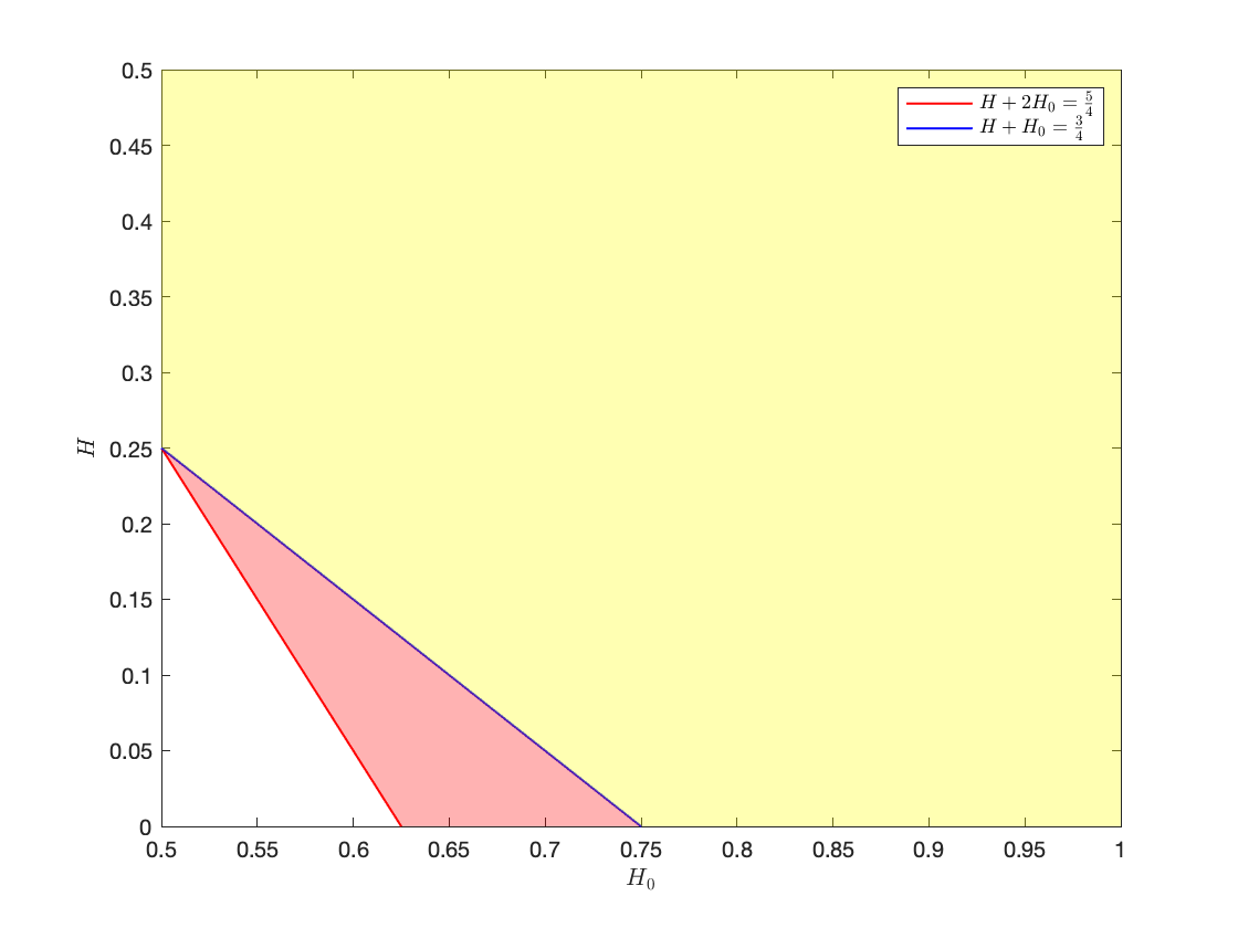
Figure 1. Hölder-Young-Brascamp-Lieb region (red) and Hardy-Littlewood-Sobolev region (yellow)

Here is our main theorem of this section.

Theorem 5.1.

Let $u(t,x)$ be the solution candidate (2.14). Suppose $d=1$, $H_{0}>\frac{1}{2}$ and $H=H_{1}<\frac{1}{2}$. If $(H_{0},H)\in\mathcal{A}_{1}\cup\mathcal{A}_{2}$, where

$$\mathcal{A}_{1}= \left\{(H_{0},H)\in(1/2,1)\times(1/20,1/4):\ 2H_{0}+H>5/4\right\}\,;$$ (5.1)

$$\mathcal{A}_{2}= \left\{(H_{0},H)\in(1/2,1)\times(0,1/20):\ 4H_{0}+12H>3\right\}\,,$$ (5.2)

then

$$\mathbb{E}[|u(t,x)|^{2}]=\sum\limits_{n=1}^{\infty}\mathbb{E}[|u_{n}(t,x)|^{2}]<+\infty.$$ (5.3)

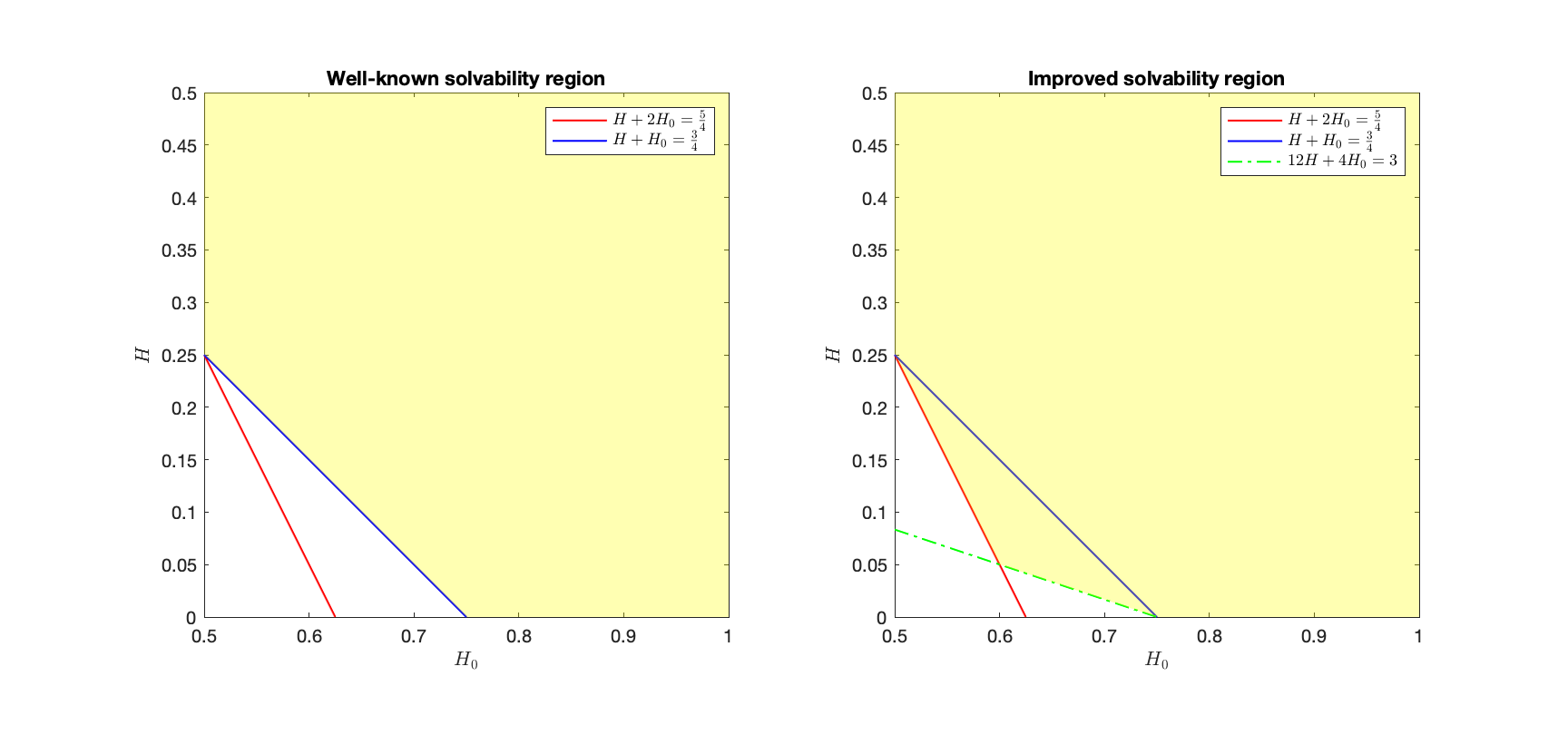
Figure 2. Solvability regions

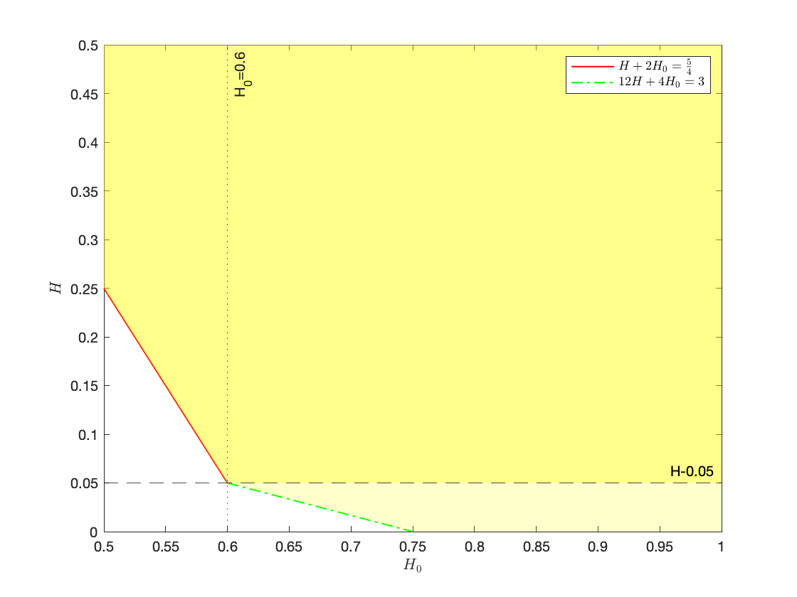
Figure 3. The dark yellow region is for region $\mathcal{A}_{1}$ and the light yellow region is for region $\mathcal{A}_{2}$

The condition $4H_{0}+12H>3$ can be written as

$$2H_{0}+H>\frac{1}{4}+\frac{5}{3}H_{0}\,,$$

which is implied by $2H_{0}+H>\frac{5}{4}$ and $H_{0}\leq 3/5$. Similarly, $4H_{0}+12H>3$ is also implied by $2H_{0}+H>\frac{5}{4}$ and $H\geq 1/20$. This combined with Corollary 4.2 imply immediately that

Corollary 5.2.

Suppose $d=1$. If $(H_{0},H)\in(\frac{1}{2},1)\times(\frac{1}{20},\frac{1}{2})$ or $(H_{0},H)\in(\frac{1}{2},\frac{3}{5})\times(0,\frac{1}{2})$, then the necessary and sufficient condition for the Itô-Wiener chaos expansion (2.14) to converge is $2H_{0}+H>\frac{5}{4}$.

Now we begin to prove Theorem 5.1.

Proof of Theorem 5.1.

For any permutation $\sigma$ of $\{1,\cdots,n\}$, recall that $\mathbb{T}_{1}(\vec{\mathbf{s}}\circ\sigma):=\{0<s_{\sigma(1)}<\cdots s_{\sigma(n)}<1\}$ and

$$\widehat{f}_{n,\sigma}^{(t,x)}(s_{1},\xi_{1},\cdots,s_{n},\xi_{n}) =\prod_{i=1}^{n}e^{-\frac{1}{2}(s_{\sigma(i+1)}-s_{\sigma(i)})|\eta_{i}^{\sigma}|^{2}}e^{-\iota x\eta_{n}^{\sigma}}{\bf 1}_{\sigma}(\vec{\mathbf{s}})$$

$$=:\widehat{f}_{n,\sigma}^{(t,x)}(\vec{\mathbf{s}},\bm{\eta}),$$

with the notations $\bm{\eta}:=(\eta_{1},\cdots,\eta_{n})$, ${\bf 1}_{\sigma}(\vec{\mathbf{s}}):={\bf 1}_{\mathbb{T}_{1}(\vec{\mathbf{s}}\circ\sigma)}={\bf 1}_{\{0<s_{\sigma(1)}<\cdots<s_{\sigma(n)}<1\}}(\vec{\mathbf{s}})$, $\eta_{i}^{\sigma}:=\xi_{\sigma(1)}+\cdots+\xi_{\sigma(i)}$ and $\widehat{f}_{n}^{(t,x)}(\cdot):=\widehat{f}_{n,\sigma}^{(t,x)}(\cdot)$. The notations involved with the variable $\vec{\mathbf{r}}$ are defined similarly.

It is not hard to see that

$$I_{n}:= \|\frac{1}{n!}\sum_{\sigma}f_{n,\sigma}^{(t,x)}(\cdot)\|^{2}_{\mathfrak{H}^{\otimes n}}$$

$$= \frac{1}{(n!)^{2}}\int_{\mathbb{R}_{+}^{2n}}\int_{\mathbb{R}^{n}}\sum_{\sigma}\widehat{f}_{n,\sigma}^{(t,x)}(\vec{\mathbf{r}},\bm{\xi})\cdot\sum_{\varsigma}\overline{\widehat{f}_{n,\varsigma}^{(t,x)}(\vec{\mathbf{s}},\bm{\xi})}\prod_{j=1}^{n}|\xi_{j}|^{1-2H}\prod_{i=1}^{n}|s_{i}-r_{i}|^{-\gamma}d\bm{\xi}d\vec{\mathbf{s}}d\vec{\mathbf{r}}$$

$${\lesssim} \sum_{\bm{\pi}}\int_{\mathbb{R}_{+}^{2n}}\int_{\mathbb{R}^{n}}\frac{1}{n!}\sum_{\sigma}\widehat{f}_{n,\sigma}^{(t,x)}(\vec{\mathbf{r}},\bm{\eta})\cdot\frac{1}{n!}\sum_{\varsigma}\overline{\widehat{f}_{n,\varsigma}^{(t,x)}(\vec{\mathbf{s}},\bm{\eta})}$$

$$\qquad\qquad\qquad\qquad\qquad\qquad\qquad\qquad\times\prod_{j=1}^{n}|\eta_{j}|^{(1-2H)\pi_{j}}\prod_{i=1}^{n}|s_{i}-r_{i}|^{-\gamma}d\bm{\eta}d\vec{\mathbf{s}}d\vec{\mathbf{r}}\,,$$

where $d\bm{\eta}=d\eta_{1}\cdots d\eta_{n}$, $\pi_{j}\in\{0,1,2\}$ and $|\bm{\pi}|=n$. Set

$$\psi_{n}(\vec{\mathbf{r}},\vec{\mathbf{s}};\bm{\eta}):=\frac{1}{n!}\sum_{\sigma}\widehat{f}_{n,\sigma}^{(t,x)}(\vec{\mathbf{r}},\bm{\eta})\cdot\frac{1}{n!}\sum_{\varsigma}\overline{\widehat{f}_{n,\varsigma}^{(t,x)}(\vec{\mathbf{s}},\bm{\eta})}$$

and

$$\Psi_{n,\bm{\tau}}(\vec{\mathbf{r}},\vec{\mathbf{s}}):= \int_{\mathbb{R}^{n}}\psi_{n}(\vec{\mathbf{r}},\vec{\mathbf{s}};\bm{\eta})\prod_{j=1}^{n}|\eta_{j}|^{\tau_{j}}d\bm{\eta}$$

with $\bm{\tau}=(\tau_{1},\cdots,\tau_{n})$ to be chosen in the following. By Hölder’s inequality with $\frac{1}{p}+\frac{1}{q}=1$, $k+k^{\prime}=1$ and $m+m^{\prime}=1$, we have

$$I_{n}\leq \sum_{\bm{\pi}}\bigg{(}\int_{\mathbb{R}_{+}^{2n}}\Psi_{n,\bm{\tau}}(\vec{\mathbf{r}},\vec{\mathbf{s}})\prod_{i=1}^{n}|s_{i}-r_{i}|^{-pm\gamma}d\vec{\mathbf{s}}d\vec{\mathbf{r}}\bigg{)}^{\frac{1}{p}}$$

$$\qquad\times\bigg{(}\int_{\mathbb{R}_{+}^{2n}}\Psi_{n,\bm{\tau^{\prime}}}(\vec{\mathbf{r}},\vec{\mathbf{s}})\prod_{i=1}^{n}|s_{i}-r_{i}|^{-qm^{\prime}\gamma}d\vec{\mathbf{s}}d\vec{\mathbf{r}}\bigg{)}^{\frac{1}{q}}$$

$$=: \sum_{\bm{\pi}}\mathcal{J}_{1}(p,m,k)\times\mathcal{J}_{2}(q,m^{\prime},k^{\prime})\,,$$ (5.4)

with $\tau_{j}=kp(1-2H)\pi_{j}$ and $\tau^{\prime}_{j}=k^{\prime}q(1-2H)\pi_{j}$. We will apply the Hölder-Young-Brascamp-Lieb inequality to $\mathcal{J}_{1}$ and the Hardy-Littlewood-Sobolev inequality to $\mathcal{J}_{2}$ separately.

Step 1: Estimate $\mathcal{J}_{1}(p,m,k)$. We shall use the Hölder-Young-Brascamp-Lieb inequality to show $\mathcal{J}_{1}:=\mathcal{J}_{1}(p,m,k)\leq C^{n}$. Firstly, we have

$$\psi_{n}(\vec{\mathbf{r}},\vec{\mathbf{s}};\bm{\eta})\leq \frac{1}{(n!)^{2}}\sum_{\sigma,\varsigma}|\widehat{f}_{n,\sigma}^{(t,x)}(\vec{\mathbf{r}},\bm{\eta})\cdot\overline{\widehat{f}_{n,\varsigma}^{(t,x)}(\vec{\mathbf{s}},\bm{\eta})}|\,.$$

An application of the Cauchy-Schwarz inequality yields

$$\mathcal{J}_{1}^{p}= \int_{\mathbb{R}_{+}^{2n}}\Psi_{n,\bm{\tau}}(\vec{\mathbf{r}},\vec{\mathbf{s}})\prod_{j=1}^{n}|s_{j}-r_{j}|^{-pm\gamma}d\vec{\mathbf{s}}d\vec{\mathbf{r}}$$

$$\leq \frac{1}{(n!)^{2}}\sum_{\sigma,\varsigma}\int_{\mathbb{R}_{+}^{2n}}\int_{\mathbb{R}^{n}}|\widehat{f}_{n,\sigma}^{(t,x)}(\vec{\mathbf{r}},\bm{\eta})\cdot\overline{\widehat{f}_{n,\varsigma}^{(t,x)}(\vec{\mathbf{s}},\bm{\eta})}|\prod_{j=1}^{n}|\eta_{j}|^{\tau_{j}}|s_{j}-r_{j}|^{-pm\gamma}d\bm{\eta}d\vec{\mathbf{s}}d\vec{\mathbf{r}}$$

$${\lesssim} \frac{1}{(n!)^{2}}\sum_{\sigma,\varsigma}\bigg{(}\int_{\mathbb{R}_{+}^{2n}}\int_{\mathbb{R}^{n}}|\widehat{f}_{n,\sigma}^{(t,x)}(\vec{\mathbf{r}},\bm{\eta})\overline{\widehat{f}_{n,\sigma}^{(t,x)}(\vec{\mathbf{s}},\bm{\eta})}|\prod_{j=1}^{n}|\eta_{j}|^{\tau_{j}}|s_{j}-r_{j}|^{-pm\gamma}d\bm{\eta}d\vec{\mathbf{s}}d\vec{\mathbf{r}}\bigg{)}^{\frac{1}{2}}$$

$$\qquad\quad\times\bigg{(}\int_{\mathbb{R}_{+}^{2n}}\int_{\mathbb{R}^{n}}|\widehat{f}_{n,\varsigma}^{(t,x)}(\vec{\mathbf{r}},\bm{\eta})\overline{\widehat{f}_{n,\varsigma}^{(t,x)}(\vec{\mathbf{s}},\bm{\eta})}|\prod_{j=1}^{n}|\eta_{j}|^{\tau_{j}}|s_{j}-r_{j}|^{-pm\gamma}d\bm{\eta}d\vec{\mathbf{s}}d\vec{\mathbf{r}}\bigg{)}^{\frac{1}{2}}$$

$$= \frac{1}{(n!)^{2}}\sum_{\sigma,\varsigma}\int_{\mathbb{R}_{+}^{2n}}\int_{\mathbb{R}^{n}}|\widehat{f}_{n}^{(t,x)}(\vec{\mathbf{r}},\bm{\eta})\overline{\widehat{f}_{n}^{(t,x)}(\vec{\mathbf{s}},\bm{\eta})}|\prod_{j=1}^{n}|\eta_{j}|^{\tau_{j}}|s_{j}-r_{j}|^{-pm\gamma}d\bm{\eta}d\vec{\mathbf{s}}d\vec{\mathbf{r}}$$

$${\lesssim} \int_{\mathbb{T}_{1}(\vec{\mathbf{s}})\times\mathbb{T}_{1}(\vec{\mathbf{r}})}\prod_{j=1}^{n}|s_{j+1}-s_{j}|^{-\frac{\varrho_{j}}{2}}|r_{j+1}-r_{j}|^{-\frac{\varrho_{j}}{2}}\times|s_{j}-r_{j}|^{-pm\gamma}d\vec{\mathbf{s}}d\vec{\mathbf{r}}\,,$$

which is bounded by $C^{n}$ under the dimension conditions of Theorem A.3 with

$$\varrho_{j}=\frac{1}{2}+\frac{\tau_{j}}{2}=\begin{cases}\frac{1}{2}\,,&\pi_{j}=0\,;\\ \frac{1}{2}+\frac{kp}{2}(1-2H)\,,&\pi_{j}=1\,;\\ \frac{1}{2}+kp(1-2H)\,,&\pi_{j}=2\,.\end{cases}$$

Similarly to the argument in the proof of Theorem 4.1, the dimension conditions will hold if the following conditions are satisfied:

$$2\Big{[}\frac{1}{4}+\frac{kp}{2}(1-2H)\Big{]}+2(2-2H^{(1)}_{0})<3\quad\text{and}\quad pm\gamma<1$$

which is equivalent to

$$1<p<\frac{5}{2k(1-2H)+8m(1-H_{0})}\quad\text{and}\quad 1<p<\frac{1}{2m(1-H_{0})}\,,$$ (5.5)

where $H_{0}^{(1)}:=1-pm(1-H_{0})$.

Step 2: Estimate $\mathcal{J}_{2}(q,m^{\prime},k^{\prime})$. We shall use the Hardy-Littlewood-Sobolev inequality to show

$$\mathcal{J}_{2}:=\mathcal{J}_{2}(q,m^{\prime},k^{\prime})\lesssim(n!)^{-\frac{2}{q}+\frac{1}{2q}+\frac{k^{\prime}}{2}(1-2H)},$$

with $\mathcal{J}_{2}(q,m^{\prime},k^{\prime})$ defined by (5). By the Cauchy-Schwarz inequality, we have

$$\Psi_{n,\bm{\tau^{\prime}}}(\vec{\mathbf{r}},\vec{\mathbf{s}})\leq\sqrt{\Psi_{n,\bm{\tau^{\prime}}}(\vec{\mathbf{r}},\vec{\mathbf{r}})}\sqrt{\Psi_{n,\bm{\tau^{\prime}}}(\vec{\mathbf{s}},\vec{\mathbf{s}})}\,.$$

We substitute this into $\mathcal{J}_{2}$ and then apply the Hardy-Littlewood-Sobolev inequality to obtain

$$\mathcal{J}_{2}= \bigg{(}\int_{\mathbb{R}_{+}^{2n}}\Psi_{n,\bm{\tau^{\prime}}}(\vec{\mathbf{r}},\vec{\mathbf{s}})\prod_{i=1}^{n}|s_{i}-r_{i}|^{-qm^{\prime}\gamma}d\vec{\mathbf{s}}d\vec{\mathbf{r}}\bigg{)}^{\frac{1}{q}}$$

$$\leq \bigg{(}\int_{\mathbb{R}_{+}^{2n}}\sqrt{\Psi_{n,\bm{\tau^{\prime}}}(\vec{\mathbf{r}},\vec{\mathbf{r}})}\sqrt{\Psi_{n,\bm{\tau^{\prime}}}(\vec{\mathbf{s}},\vec{\mathbf{s}})}\prod_{i=1}^{n}|s_{i}-r_{i}|^{-qm^{\prime}\gamma}d\vec{\mathbf{s}}d\vec{\mathbf{r}}\bigg{)}^{\frac{1}{q}}$$

$${\lesssim} \bigg{(}\int_{\mathbb{R}_{+}^{n}}\Big{|}\Psi_{n,\bm{\tau^{\prime}}}(\vec{\mathbf{s}},\vec{\mathbf{s}})\Big{|}^{\frac{1}{2H^{(2)}_{0}}}d\vec{\mathbf{s}}\bigg{)}^{\frac{2H^{(2)}_{0}}{q}}\,,$$

where $H_{0}^{(2)}:=1-qm^{\prime}(1-H_{0})$ and we should require $qm^{\prime}\gamma<1$. Recall that ${\gamma}=2-2H_{0}$, then

$$qm^{\prime}\gamma<1\Leftrightarrow 1<q<\frac{1}{2m^{\prime}(1-H_{0})}\,.$$ (5.6)

Notice that

$$\Psi_{n,\bm{\tau^{\prime}}}(\vec{\mathbf{s}},\vec{\mathbf{s}})= \int_{\mathbb{R}^{n}}\bigg{|}\frac{1}{n!}\sum_{\sigma}\widehat{f}_{n,\sigma}^{(t,x)}(\vec{\mathbf{s}},\bm{\eta})\cdot\frac{1}{n!}\sum_{\varsigma}\overline{\widehat{f}_{n,\varsigma}^{(t,x)}(\vec{\mathbf{s}},\bm{\eta})}\bigg{|}\prod_{j=1}^{n}|\eta_{j}|^{\tau^{\prime}_{j}}d\bm{\eta}$$

$$= \int_{\mathbb{R}^{n}}\bigg{|}\frac{1}{(n!)^{2}}\sum_{\sigma,\varsigma}\widehat{f}_{n,\sigma}^{(t,x)}(\vec{\mathbf{s}},\bm{\eta})\cdot\overline{\widehat{f}_{n,\varsigma}^{(t,x)}(\vec{\mathbf{s}},\bm{\eta})}\bigg{|}\prod_{j=1}^{n}|\eta_{j}|^{\tau^{\prime}_{j}}d\bm{\eta}$$

$$= \int_{\mathbb{R}^{n}}\frac{1}{(n!)^{2}}\sum_{\sigma}|\widehat{f}_{n,\sigma}^{(t,x)}(\vec{\mathbf{s}},\bm{\eta})|^{2}\prod_{j=1}^{n}|\eta_{j}|^{\tau^{\prime}_{j}}d\bm{\eta}\,,$$ (5.7)

where the last equality follows from

$${\bf 1}_{\sigma}(\vec{\mathbf{s}})\cdot{\bf 1}_{\varsigma}(\vec{\mathbf{s}})=\begin{cases}0\,,&\sigma\neq\varsigma\,;\\ {\bf 1}_{\sigma}(\vec{\mathbf{s}})\,,&\sigma=\varsigma\,.\end{cases}$$

Hence, we have

$$\int_{\mathbb{R}_{+}^{n}}\Big{|}\Psi_{n,\bm{\tau^{\prime}}} (\vec{\mathbf{s}},\vec{\mathbf{s}})\Big{|}^{\frac{1}{2H^{(2)}_{0}}}d\vec{\mathbf{s}}$$

$$= \frac{1}{(n!)^{\frac{1}{H^{(2)}_{0}}}}\int_{\mathbb{R}_{+}^{n}}\bigg{|}\int_{\mathbb{R}^{n}}\sum_{\sigma}|\widehat{f}_{n,\sigma}^{(t,x)}(\vec{\mathbf{s}},\bm{\eta})|^{2}\prod_{j=1}^{n}|\eta_{j}|^{\tau^{\prime}_{j}}d\bm{\eta}\bigg{|}^{\frac{1}{2H^{(2)}_{0}}}d\vec{\mathbf{s}}$$

$$= \frac{1}{(n!)^{\frac{1}{H^{(2)}_{0}}}}\sum_{\sigma^{\prime}}\int_{\mathbb{T}_{1}(\vec{\mathbf{s}}\circ\sigma^{\prime})}\bigg{|}\int_{\mathbb{R}^{n}}\sum_{\sigma}|\widehat{f}_{n,\sigma}^{(t,x)}(\vec{\mathbf{s}},\bm{\eta})|^{2}\prod_{j=1}^{n}|\eta_{j}|^{\tau^{\prime}_{j}}d\bm{\eta}\bigg{|}^{\frac{1}{2H^{(2)}_{0}}}d\vec{\mathbf{s}}$$

$$= \frac{1}{(n!)^{\frac{1}{H^{(2)}_{0}}}}\sum_{\sigma}\int_{\mathbb{T}_{1}(\vec{\mathbf{s}}\circ\sigma)}\bigg{|}\int_{\mathbb{R}^{n}}|\widehat{f}_{n,\sigma}^{(t,x)}(\vec{\mathbf{s}},\bm{\eta})|^{2}\prod_{j=1}^{n}|\eta_{j}|^{\tau^{\prime}_{j}}d\bm{\eta}\bigg{|}^{\frac{1}{2H^{(2)}_{0}}}d\vec{\mathbf{s}}$$

$${\lesssim} \frac{1}{(n!)^{\frac{1}{H^{(2)}_{0}}}}\sum_{\sigma}\int_{\mathbb{T}_{1}(\vec{\mathbf{s}}\circ\sigma)}\prod_{i=1}^{n}|s_{\sigma(i+1)}-s_{\sigma(i)}|^{-\frac{\varrho^{\prime}_{j}}{2H^{(2)}_{0}}}d\vec{\mathbf{s}}$$ (5.8)

with $\varrho^{\prime}_{j}$ being defined by

$$\varrho^{\prime}_{j}=\frac{1}{2}+\frac{\tau^{\prime}_{j}}{2}=\begin{cases}\frac{1}{2}\,,&\pi_{j}=0\,;\\ \frac{1}{2}+\frac{k^{\prime}q}{2}(1-2H)\,,&\pi_{j}=1\,;\\ \frac{1}{2}+k^{\prime}q(1-2H)\,,&\pi_{j}=2\,.\end{cases}$$

The finiteness of (5) requires that for $j=1,\cdots,n$, $\frac{\varrho^{\prime}_{j}}{2H^{(2)}_{0}}$ satisfies the following Hardy-Littlewood-Sobolev conditions:

$$\frac{\varrho^{\prime}_{j}}{2H^{(2)}_{0}}<1\Leftrightarrow \ \frac{\frac{1}{2}+k^{\prime}q(1-2H)}{2H^{(2)}_{0}}<1$$

$$\Leftrightarrow \ \ 1<q<\frac{3}{2k^{\prime}(1-2H)+4m^{\prime}(1-H_{0})}\,.$$ (5.9)

Under the above condition we have

$$\bigg{[}\int_{\mathbb{R}_{+}^{n}}\Big{|}\Psi_{n,\bm{\tau^{\prime}}}^{(q)} (\vec{\mathbf{s}},\vec{\mathbf{s}})\Big{|}^{\frac{1}{2H^{(2)}_{0}}}d\vec{\mathbf{s}}\bigg{]}^{\frac{2H^{(2)}_{0}}{q}}$$

$${\lesssim} \frac{C^{n}}{(n!)^{\frac{2}{q}}}\bigg{[}n!\cdot\frac{\prod_{i=1}^{n}\Gamma(1-\varrho^{\prime}_{j}/2H^{(2)}_{0})}{\Gamma(n-\sum_{j=1}^{n}\varrho^{\prime}_{j}/2H^{(2)}_{0}+1)}\bigg{]}^{\frac{2H^{(2)}_{0}}{q}}$$

$${\lesssim} C^{n}(n!)^{-\frac{2}{q}+[\frac{1}{2q}+\frac{k^{\prime}}{2}(1-2H)]}$$

where the last inequality follows from the Stirling formula and the fact that

$$\sum_{j=1}^{n}\varrho^{\prime}_{j}\sim n\Big{[}\frac{1}{2}+\frac{k^{\prime}q}{2}(1-2H)\Big{]}\,.$$

As a result,

$$\mathbb{E}[u(t,x)^{2}]\leq \sum_{n=0}^{\infty}n!\sum_{\bm{\pi}}\mathcal{J}_{1}\times\mathcal{J}_{2}$$

$$\leq \sum_{n=0}^{\infty}C^{n}(n!)^{1-\frac{2}{q}+[\frac{1}{2q}+\frac{k^{\prime}}{2}(1-2H)]}\,.$$

This proves $\mathbb{E}[u(t,x)^{2}]<\infty$ if

$$1-\frac{2}{q}+\Big{[}\frac{1}{2q}+\frac{k^{\prime}}{2}(1-2H)\Big{]}<0\Leftrightarrow 1<q<\frac{3}{k^{\prime}(1-2H)+2}\,.$$ (5.10)

Step 3: Constraints on $p$ ($q$), $m$ ($m^{\prime}$), and $k$ ($k^{\prime}$). The conditions (5.6) and (5) are summarized as

$$1<q<\frac{3}{2k^{\prime}(1-2H)+4m^{\prime}(1-H_{0})}\quad\text{and}\quad 1<q<\frac{1}{2m^{\prime}(1-H_{0})}\,.$$ (5.11)

Recall that in Step 2 and Step 3, to guarantee $\mathbb{E}[|u(t,x)|^{2}]<+\infty$, we must have

$$1<p<\frac{5}{2k(1-2H)+8m(1-H_{0})}\wedge\frac{1}{2m(1-H_{0})}\,;$$ (5.12)

$$1<q<\frac{3}{2k^{\prime}(1-2H)+4m^{\prime}(1-H_{0})}\wedge\frac{1}{2m^{\prime}(1-H_{0})}\,;$$ (5.13)

$$1<q<\frac{3}{k^{\prime}(1-2H)+2}\,.$$ (5.14)

To find the conditions on $H$, $H_{0}$ so that (5.12)-(5.14) are satisfied, we first get rid the symbol “$\wedge$” in the above first two inequalities (5.12) and (5.13). To this end, we consider the following four cases:

$$\begin{cases}\hbox{Case 1}:\ \frac{5}{2k(1-2H)+8m(1-H_{0})}<\frac{1}{2m(1-H_{0})}\,,\quad\frac{3}{2k^{\prime}(1-2H)+4m^{\prime}(1-H_{0})}<\frac{1}{2m^{\prime}(1-H_{0})}\,;\\ \hbox{Case 2}:\ \frac{5}{2k(1-2H)+8m(1-H_{0})}<\frac{1}{2m(1-H_{0})}\,,\quad\frac{3}{2k^{\prime}(1-2H)+4m^{\prime}(1-H_{0})}>\frac{1}{2m^{\prime}(1-H_{0})}\,;\\ \hbox{Case 3}:\ \frac{5}{2k(1-2H)+8m(1-H_{0})}>\frac{1}{2m(1-H_{0})}\,,\quad\frac{3}{2k^{\prime}(1-2H)+4m^{\prime}(1-H_{0})}<\frac{1}{2m^{\prime}(1-H_{0})}\,;\\ \hbox{Case 4}:\ \frac{5}{2k(1-2H)+8m(1-H_{0})}>\frac{1}{2m(1-H_{0})}\,,\quad\frac{3}{2k^{\prime}(1-2H)+4m^{\prime}(1-H_{0})}>\frac{1}{2m^{\prime}(1-H_{0})}\,.\\ \end{cases}$$ (5.15)

We shall deal with the Case 1 in details and other cases are similar.

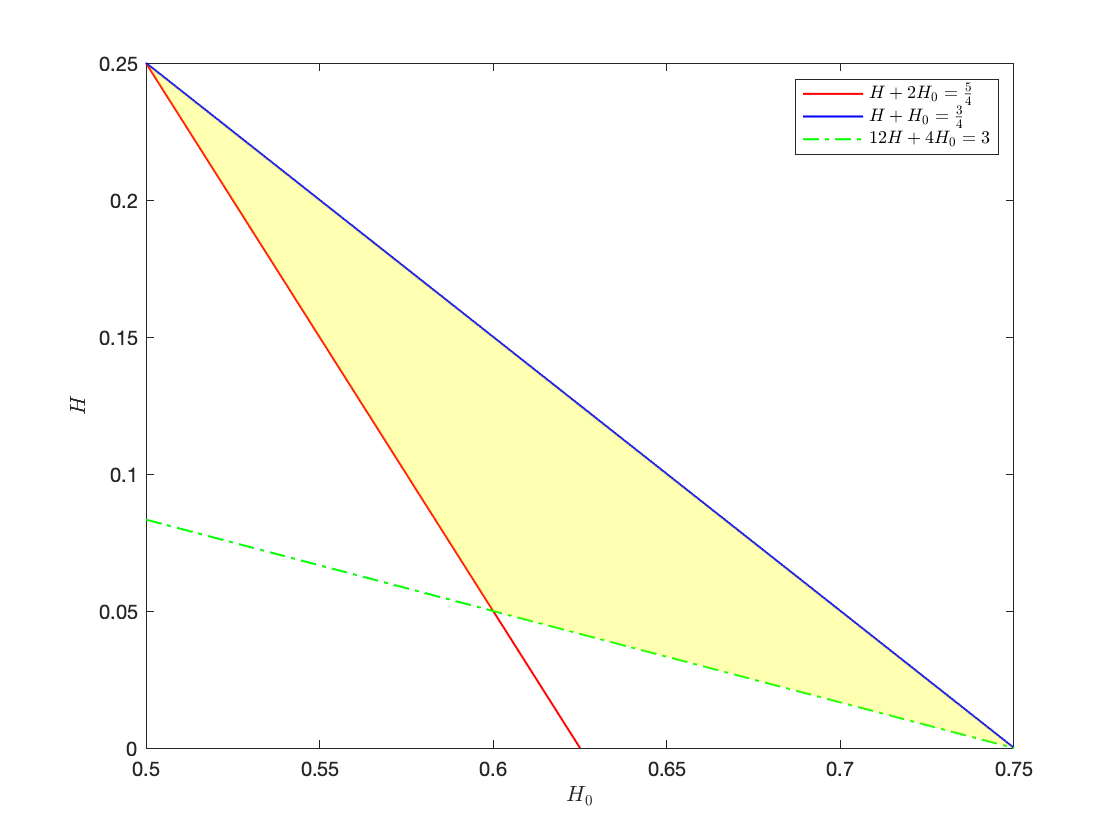
Figure 4. Case 1

Case 1: In this case, the constraints (5.12)-(5.14) on $p,\ q$ become the following conditions:

$$\begin{cases}&1<q<\frac{3}{k^{\prime}(1-2H)+2}\,;\\ &1<q<\frac{3}{2k^{\prime}(1-2H)+4m^{\prime}(1-H_{0})}<\frac{1}{2m^{\prime}(1-H_{0})}\,;\\ &1<p<\frac{5}{2k(1-2H)+8m(1-H_{0})}<\frac{1}{2m(1-H_{0})}\,.\end{cases}$$ (5.16)

Denote

$$\mathcal{S}:= \left\{(H,H_{0})\in(0,\frac{1}{4})\times(\frac{1}{2},\frac{3}{4}):\ H+2H_{0}>\frac{5}{4},\ H+H_{0}\leq\frac{3}{4},\ 12H+4H_{0}>3\right\}.$$ (5.17)

We shall show that for any $(H,H_{0})\in\mathcal{S}$, there exist $p,q\in[1,\infty)$, and $m,m^{\prime}\in[0,1],\ k,k^{\prime}\in[0,1]$ such that conditions (5.16) hold. For any arbitrarily small $\varepsilon>0$, let us choose

$$q=\frac{3}{k^{\prime}(1-2H)+2}-\varepsilon,$$ (5.18)

$$p=\frac{q}{q-1}=\frac{3-\varepsilon}{1-k^{\prime}(1-2H)-\varepsilon},$$ (5.19)

$$m^{\prime}=\frac{2-k^{\prime}(1-2H)}{4(1-H_{0})}.$$ (5.20)

Thus it suffices to show that for any $(H,H_{0})\in\mathcal{S}$, there exists $k^{\prime}\in[0,1]$ such that the parameters $(p,q,m^{\prime})$ given by (5.18)-(5.20) satisfy conditions (5.16) for sufficiently small $\varepsilon>0$.

Firstly, we need to ensure $p,q\geq 1$ and $0\leq m^{\prime}\leq 1$. Note that

$$q\geq 1\Leftrightarrow k^{\prime}\leq\frac{1-2\varepsilon}{(1-2H)(1+\varepsilon)}\sim\frac{1}{1-2H}\,,$$

which is implied by $k^{\prime}\leq 1$. Now $p\geq 1$ is equivalent to $q\geq 1$. Besides,

$$0\leq m^{\prime}\leq 1\Leftrightarrow k^{\prime}\geq\frac{4H_{0}-2}{1-2H}\,.$$ (5.21)

In order to be able to find a $k^{\prime}\in[0,1]$ so that the above inequality holds true we need

$$\frac{4H_{0}-2}{1-2H}\leq 1\Leftrightarrow H+2H_{0}\leq\frac{3}{2},$$

which holds for $(H,H_{0})\in\mathcal{S}$ since $H+H_{0}\leq\frac{3}{4}$ and $H_{0}<\frac{3}{4}$.

Next, we shall verify the conditions (5.16) with the $p,\ q$ and $m^{\prime}$ given by (5.18)-(5.20). It is clear that we can take $\varepsilon=0$.

1. The first line of (5.16) holds obviously with the choice of $q$ in (5.18).

2. For the $q$ defined by (5.18) we now show the second line of (5.16):

   $$q<\frac{3}{2k^{\prime}(1-2H)+4m^{\prime}(1-H_{0})}\,,$$

   which is equivalent to

   $$\frac{3}{k^{\prime}(1-2H)+2}\leq\frac{3}{2k^{\prime}(1-2H)+4m^{\prime}(1-H_{0})}$$

   $$\Leftrightarrow\ m^{\prime}\leq\frac{2-k^{\prime}(1-2H)}{4(1-H_{0})}\,.$$

   This holds with the choice of $m^{\prime}$ in (5.20).

3. The third inequality of second line in (5.16) is

   $$\frac{3}{2k^{\prime}(1-2H)+4m^{\prime}(1-H_{0})}<\frac{1}{2m^{\prime}(1-H_{0})}$$

   which is equivalent to

   $$m^{\prime}(1-H_{0})<k^{\prime}(1-2H)\,.$$ (5.22)

   By using the definition (5.20) of $m^{\prime}$ this is equivalent to

   $$\frac{2}{5(1-2H)}<k^{\prime}<1\,.$$ (5.23)

4. The second inequality of the third line of (5.16), by choice of $p$ in (5.19), is equivalent to

   $$25-12(H+2H_{0})<k^{\prime}(1-2H)+24m^{\prime}(1-H_{0})\,.$$

   With $m^{\prime}$ defined in (5.20) this can be rewritten as

   $$0<k^{\prime}<\frac{12(H+2H_{0})-13}{5(1-2H)}.$$ (5.24)

5. Now we consider the third inequality in the last line of (5.16). Noticing that $k=1-k^{\prime}$ and $m=1-m^{\prime}$ and substituting the value of $m^{\prime}$, this yields

   $$0<k^{\prime}<\frac{2+4(H_{0}-2H)}{5(1-2H)}.$$ (5.25)

In conclusion, if $k^{\prime}$ satisfies the constraints (5.28), (5.23), (5.24) and (5.25), then (5.16) will be satisfied. We can summarize the conditions satisfied by $k^{\prime}$ as follows.

$$\left\{\frac{2}{5(1-2H)}\vee\frac{4H_{0}-2}{1-2H}\right\}<k^{\prime}<\left\{\frac{12(H+2H_{0})-13}{5(1-2H)}\wedge\frac{2+4(H_{0}-2H)}{5(1-2H)}\wedge 1\right\}\,.$$ (5.26)

Notice that

$$12(H+2H_{0})-13\leq 2+4(H_{0}-2H)\Leftrightarrow H+H_{0}\leq\frac{3}{4}$$

and

$$\frac{12(H+2H_{0})-13}{5(1-2H)}\leq 1\Leftrightarrow 11H+12H_{0}\leq 9,$$

which holds under the condition $H+H_{0}\leq\frac{3}{4}$. Thus, on the set $\mathcal{S}$ the condition (5.26) is reduced to

$$\left\{\frac{2}{5(1-2H)}\vee\frac{4H_{0}-2}{1-2H}\right\}<k^{\prime}<\frac{12(H+2H_{0})-13}{5(1-2H)}.$$ (5.27)

Finally, it remains to show that when $(H,H_{0})\in\mathcal{S}$, there is $k^{\prime}$ satisfying (5.27), or

$$\left\{\frac{2}{5(1-2H)}\vee\frac{4H_{0}-2}{1-2H}\right\}\leq\frac{12(H+2H_{0})-13}{5(1-2H)}.$$ (5.28)

We shall prove the above inequality assuming $H_{0}\leq 3/5$ and $H_{0}>3/5$ respectively. First, let us assume $H_{0}\leq\frac{3}{5}$. In this case, we have $\frac{2}{5(1-2H)}\leq\frac{4H_{0}-2}{1-2H}$. Then (5.28) becomes

$$\frac{2}{5(1-2H)}<\frac{12(H+2H_{0})-13}{5(1-2H)}\Leftrightarrow H+2H_{0}>\frac{5}{4}\,$$

which holds true since $(H,H_{0})\in\mathcal{S}$. Next, we assume $H_{0}>\frac{3}{5}$ which means $\frac{2}{5(1-2H)}>\frac{4H_{0}-2}{1-2H}$. In this case, (5.28) becomes

$$\frac{4H_{0}-2}{1-2H}<\frac{12(H+2H_{0})-13}{5(1-2H)}\Leftrightarrow 12H+4H_{0}>3\,.$$

Therefore, for any given $(H,H_{0})\in\mathcal{S}$ we can choose $k^{\prime}$ appropriately so that the condition (5.27) holds.

Case 2-Case 4: These cases can be treated in the same spirit as Case 1. However, it turns out that the solvability region can not the enlarged. So, we omit the details.

As a result, on the region $\mathcal{S}$ (see Figure 4), we have

$$\mathbb{E}[u(t,x)^{2}]=\sum\limits_{n=1}^{\infty}\mathbb{E}[|u_{n}(t,x)|^{2}]<+\infty.$$

Since the above convergence is proved in [15] when $H_{0}+H>3/4$, we complete the proof.

∎

Appendix A Some lemmas

Lemma A.1.

Let $0<{\alpha},{\beta}<1$ with ${\alpha}+{\beta}>1$. Then there is a constant $c\geq 1$ independent of ${\varepsilon}>0$ such that for all $x\in(0,3{\varepsilon})$,

$$c^{-1}x^{1-({\alpha}+{\beta})}\leq\int_{0}^{\varepsilon}u^{-{\alpha}}(u+x)^{-{\beta}}du\leq cx^{1-({\alpha}+{\beta})}.$$ (A.1)

This lemma can be found in [15] and the following lemma can be found in [28].

Lemma A.2 (Hardy-Littlewood-Sobolev inequality).

For any $\varphi\in L^{1/H_{0}}(\mathbb{R}^{n})$, it holds

$$\int_{\mathbb{R}^{n}}\int_{\mathbb{R}^{n}}\varphi(\vec{\mathbf{r}})\varphi(\vec{\mathbf{s}})\prod_{i=1}^{n}|s_{i}-r_{i}|^{2H_{0}-2}d\vec{\mathbf{r}}d\vec{\mathbf{s}}\leq C_{H_{0}}\left(\int_{\mathbb{R}^{n}}|\varphi(\vec{\mathbf{r}})|^{1/H_{0}}d\vec{\mathbf{r}}\right)^{2H_{0}},$$ (A.2)

where $C_{H_{0}}>0$.

The Hölder-Young-Brascamp-Lieb type inequality has been studied and extended by various groups after the seminar work of Brascamp and Lieb [9]. We refer [1, Appendix A] and the references therein to the readers on this interesting topic. Below we present the homogeneous and non-homogeneous Hölder-Young-Brascamp-Lieb inequalities that we are going to use in this work. Let $\mathcal{H}$, $\mathcal{H}_{1}$,…, $\mathcal{H}_{m}$, be finite dimensional Hilbert spaces equipped with the corresponding Lebesgue measure $\mu(\cdot)$. For $j=1,\cdots,m$, let $f_{j}:\mathcal{H}_{j}\to\mathbb{R}_{+}$ be nonnegative satisfying $f_{j}\in L^{p_{j}}(\mu)$ for $p_{1},\cdots,p_{m}\in[1,\infty)$ and let $l_{j}:\mathcal{H}\to\mathcal{H}_{j}$ be surjective linear transformations.

We consider the (local) multilinear functional

$$\Lambda(f_{1},\dots,f_{m}):=\int\prod_{j=1}^{m}f_{j}(l_{j}(\mathbf{x}))\prod_{j=1}^{n}d\mu(x_{j})\,,$$ (A.3)

and the Hölder-Young-Brascamp-Lieb type inequality

$$|\Lambda(f_{1},\dots,f_{m})|\leq K_{\mathcal{H}}\prod_{j=1}^{m}\|f_{j}\|_{L^{p_{j}}(\mu)}\,,$$ (A.4)

for some constant positive finite $K_{\mathcal{H}}$. There are many works concerning the conditions so that (A.4) holds true. We shall use two fo them: the nonhomogeneous Hölder-Young-Brascamp-Lieb inequality borrowed from [8, Theorem 2.2] (see also [7]).

Theorem A.3 (Nonhomogeneous Hölder-Young-Brascamp-Lieb inequality).

Let $\mathcal{H}$, $\mathcal{H}_{1}$,…, $\mathcal{H}_{m}$, $f_{j}\in L^{p_{j}}(\mu)$ be as above. Consider a local version of (A.3)

$$\Lambda_{loc}(f_{1},\dots,f_{m}):=\int_{\mathbf{x}\in\mathcal{H}:|\mathbf{x}|\leq 1}\prod_{j=1}^{m}f_{j}(l_{j}(\mathbf{x}))\prod_{j=1}^{n}d\mu(x_{j})\,.$$ (A.5)

A necessary and sufficient condition for Hölder-Young-Brascamp-Lieb type inequality (A.4) holds for $\Lambda_{loc}$ with $0<K_{\mathcal{H}}<\infty$ for all nonnegative measurable functions $f_{j}$ is that every subspace $V\subseteq\mathcal{H}$ satisfies the dimension condition

$$codim_{\mathcal{H}}(V)\geq\sum_{j}p_{j}^{-1}codim_{\mathcal{H}_{j}}(l_{j}(V))\,.$$ (A.6)

Using the above theorem, we can show an important ingredient in the proof of Theorem 4.1.

Lemma A.4.

Under conditions (4.1) of Theorem 4.1, the following dimensional conditions hold when $co\dim_{\mathcal{H}}(V)=1,2,3,4$:

$$co\dim_{\mathcal{H}}(V)\geq\sum\limits_{j=1}^{6}z_{j}\cdot co\dim_{\mathcal{H}_{j}}(l_{j}(V))\,.$$

Proof.

We show the lemma for $co\dim=1,2,3,4$ separately.

Case 1: $co\dim_{\mathcal{H}}(V)=1$, i.e. $\dim_{\mathcal{H}}(V)=3$. In this case, we only need to consider ${\rm rank}([l_{j}]_{j\in J})=1$, i.e. $|J|=1$. In this case the dimension condition (4.22) holds since $z_{j}\leq 1$ ($j=1,\cdots,6$) from (4.23).

Case 2: $co\dim_{\mathcal{H}}(V)=2$, i.e. $\dim_{\mathcal{H}}(V)=2$. We shall choose $J$ such that ${\rm rank}([l_{j}]_{j\in J})=2$.

Note that we only have to deal with $|J|=3$ since the dimension condition (4.22) automatically holds for $|J|=2$ and it is impossible to have ${\rm rank}([l_{j}]_{j\in J})=3$ for $|J|=4,5,6$. The only possible case is ${\rm rank}([l_{3},l_{4},l_{6}])=2$. Then, the condition (4.22) in this case is equivalent to

$$2\,\geq z_{3}+z_{4}+z_{6}$$

$$> \rho_{2}+\rho_{2}+\gamma$$

$$= (\frac{3}{2}d+\frac{1}{2}{\beta}^{*}-2|H|-{\alpha}_{2})+2-2H_{0}$$

$$\Leftrightarrow\qquad |H|+2H_{0}>d+(\frac{1}{2}d-|H|+\frac{1}{2}{\beta}^{*})-{\alpha}_{2}\,.$$ (A.7)

Since ${\alpha}_{2}\in\{\frac{1}{2}d-|H|+\frac{1}{2}{\beta}^{*},d-2|H|+{\beta}^{*}\}$, it is obvious that (A) holds under the condition

$$|H|+2H_{0}>d.$$ (A.8)

Case 3: $co\dim_{\mathcal{H}}(V)=3$, i.e. $\dim_{\mathcal{H}}(V)=1$. We shall choose $J$ such that ${\rm rank}([l_{j}]_{j\in J})=3$.

For $|J|=3$, the dimension condition (4.22) hold automatically since $z_{i}\leq 1$ for $i=1,\cdots,6$. Moreover, it is impossible to get ${\rm rank}([l_{j}]_{j\in J})=3$ for $|J|=5,6$ by computation of the relevant ranks. Thus, we only need to consider $|J|=4$. By a simple analysis, we know that there are four cases:

$${\rm rank}([l_{1},l_{2},l_{5},l_{6}])={\rm rank}([l_{1},l_{3},l_{4},l_{6}])$$

$$={\rm rank}([l_{2},l_{3},l_{4},l_{6}])={\rm rank}([l_{3},l_{4},l_{6},l_{5}])=3\,.$$

We treat $J=\{1,2,5,6\}$ as an example. The rest is similar and we omit the details.

Now, we have ${\rm rank}([l_{1},l_{2},l_{5},l_{6}])=3$, $\dim(\cap_{j=1,2,5,6}\ker(l_{j}))=1$ and $co\dim_{\mathcal{H}}(V)=3$. In fact, we can obtain that $V=span\{(1,1,1,1)\}=\cap_{j=1,2,5,6}\ker(l_{j})$ and

$$co\dim_{\mathcal{H}_{1}}(l_{1}(V))=1\,,co\dim_{\mathcal{H}_{3}}(l_{3}(V))=0\,,co\dim_{\mathcal{H}_{5}}(l_{5}(V))=1\,,$$

$$co\dim_{\mathcal{H}_{2}}(l_{2}(V))=1\,,co\dim_{\mathcal{H}_{4}}(l_{4}(V))=0\,,co\dim_{\mathcal{H}_{6}}(l_{6}(V))=1\,.$$

Then, in this case the condition (4.22) is analogous to

$$3\,\geq z_{1}+z_{2}+z_{5}+z_{6}$$

$$> \rho_{1}+\rho_{1}+\gamma+\gamma$$

$$= (\frac{3}{2}d_{*}-2H_{*})+4-4H_{0}\,.$$ (A.9)

It is easy to see that (A) holds under the third condition of (4.1) :

$$H_{*}+2H_{0}>\frac{3}{4}d_{*}+\frac{1}{2}.$$ (A.10)

Case 4: $co\dim_{\mathcal{H}}(V)=4$, i.e. $\dim_{\mathcal{H}}(V)=0$. We shall choose $J$ such that ${\rm rank}([l_{j}]_{j\in J})=4$.

Obviously, we only need to consider $|J|=4,5,6$. We first deal with $|J|=6$. This means

$$V=\bigcap_{j=1}^{6}\ker(l_{j})=\{0,0,0,0\}\,.$$

Thus, the dimensional condition (4.22) in this case is equivalent to

$$4\,\geq z_{1}+z_{2}+z_{3}+z_{4}+z_{5}+z_{6}$$

$$> \rho_{1}+\rho_{1}+\rho_{2}+\rho_{2}+\gamma+\gamma$$

$$= (\frac{3}{2}d_{*}-2H_{*})+2(2-2H_{0})$$

$$+(\frac{3}{2}d+\frac{1}{2}{\beta}^{*}-2|H|-{\alpha}_{2}).$$

$$\Leftrightarrow\ \ |H|+2H_{*}+4H_{0}>d+\frac{3}{2}d_{*}+(\frac{1}{2}d-|H|+\frac{1}{2}{\beta}^{*}-{\alpha}_{2}).$$ (A.11)

Since ${\alpha}_{2}\in\{\frac{1}{2}d-|H|+\frac{1}{2}{\beta}^{*},d-2|H|+{\beta}^{*}\}$, we know (A.11) holds under the fourth condition of (4.1):

$$|H|+2H_{*}+4H_{0}>d+\frac{3}{2}d_{*}.$$ (A.12)

When $|J|=4,5$, the corresponding dimension conditions (4.22) can be implied by (A.11).

Thus, the proof of the lemma is complete. ∎

Now we give some estimations for the alternative proof of sufficiency of Theorem 4.1.

Lemma A.5.

For any ${\alpha},{\beta},{\gamma}\in(0,1)$ and $a,b\in\mathbb{R}$ denote

$$\mathfrak{B}_{1}(a,b):=\int_{0}^{\frac{1}{2}}u^{-\beta}(1-u)^{-{\alpha}}|au-b|^{-{\gamma}}du\,;$$ (A.13)

$$\mathfrak{B}_{2}(a,b):=\int_{\frac{1}{2}}^{1}u^{-{\beta}}(1-u)^{-{\alpha}}|au-b|^{-{\gamma}}du.$$ (A.14)

Then

$$\mathfrak{B}_{1}(a,b){\lesssim}\begin{cases}|a|^{-q}|b|^{-{\gamma}+q}\\ \qquad\qquad\qquad\hbox{for any $q\in[0,1-{\beta}]$ }\quad\hbox{if ${\beta}+{\gamma}>1$};\\ (|a|+|b|)^{-{\gamma}}{\lesssim}|a|^{-q_{1}}|b-a|^{-q_{2}}|b|^{-{\gamma}+q_{1}+q_{2}}\\ \qquad\qquad\qquad\hbox{for any $q_{1},q_{2},q_{1}+q_{2}\in[0,{\gamma}]$}\quad\hbox{if ${\beta}+{\gamma}<1$},\\ \end{cases}$$ (A.15)

and

$$\mathfrak{B}_{2}(a,b){\lesssim}\begin{cases}|a|^{-q}|b-a|^{-{\gamma}+q}\\ \qquad\qquad\qquad\hbox{for any $q\in[0,1-{\alpha}]$ }\quad\hbox{if ${\alpha}+{\gamma}>1$};\\ (|a|+|b-a|)^{-{\gamma}}{\lesssim}|a|^{-q_{1}}|b-a|^{-q_{2}}|b|^{-{\gamma}+q_{1}+q_{2}}\\ \qquad\qquad\qquad\hbox{for any $q_{1},q_{2},q_{1}+q_{2}\in[0,{\gamma}]$}\quad\hbox{if ${\alpha}+{\gamma}<1$}.\\ \end{cases}$$ (A.16)

Proof.

First let ${\beta}+{\gamma}>1$. Since for $x\geq 0,$ ${\beta}\in(0,1)$, ${\gamma}\in(0,1)$ it holds that

$$\int_{0}^{x}|\xi|^{-{\beta}}|1-\xi|^{-{\gamma}}d\xi\ {\lesssim}|x|^{-{\beta}+1}\wedge 1\,.$$

Then for any $\rho_{1}\in[0,1]$,

$$\int_{0}^{\frac{1}{2}} w^{-{\beta}}(1-w)^{-{\alpha}}|{a}w-b|^{-\gamma}dw$$

$${\lesssim}\int_{0}^{\frac{1}{2}}w^{-{\beta}}|aw-b|^{-\gamma}dw$$

$${\lesssim}|b|^{-{\gamma}}\int_{0}^{\frac{1}{2}}w^{-{\beta}}\left|\frac{|a|}{|b|}w-1\right|^{-{\gamma}}dw$$

$${\lesssim}|b|^{-\gamma-{\beta}+1}\cdot|{a}|^{{\beta}-1}\times\int_{0}^{\frac{|{a}|}{2|b|}}\xi^{-{\beta}}|1-\xi|^{-\gamma}d\xi$$

$${\lesssim}|b|^{-\gamma-{\beta}+1}\cdot|{a}|^{{\beta}-1}\cdot\left(\frac{|{a}|}{|b|}\wedge 1\right)^{-{\beta}+1}$$

$${\lesssim}|b|^{-\gamma-{\beta}+1}\cdot|{a}|^{{\beta}-1}\cdot\left(\frac{|{a}|}{|b|}\right)^{(-{\beta}+1)\rho_{1}}$$

$$=|{a}|^{-q_{1}}|b|^{-\gamma+q_{1}}\,,$$ (A.17)

where $q_{1}=(1-{\beta})(1-\rho_{1})\in[0,1-{\beta}]$ and we make substitution $\xi=\frac{|{a}|}{|b|}w$ in the third inequality. Here we need that ${\beta},\ \gamma\in(0,1),\ {\beta}+\gamma>1$.

Make substitution $\widetilde{w}=1-w$. Then for $0\leq\rho_{2}\leq 1$,

$$\int_{\frac{1}{2}}^{1} |1-w|^{-{\alpha}}w^{-{\beta}}|w-b_{v}|^{-\gamma}dw$$

$$=\int_{0}^{\frac{1}{2}}\widetilde{w}^{-{\alpha}}|1-\widetilde{w}|^{-{\beta}}|{a}-b-{a}\widetilde{w}|^{-\gamma}d\widetilde{w}\,.$$ (A.18)

This can be used to show the first inequality in (A.16).

Now if ${\beta}\in(0,1)$, ${\gamma}\in(0,1)$ and ${\beta}+{\gamma}<1$, then

$$\int_{0}^{x}|\xi|^{-{\beta}}|1-\xi|^{-{\gamma}}d\xi\ {\lesssim}\frac{|x|^{-{\beta}+1}(1+|x|^{1-{\beta}-{\gamma}})}{1+|x|^{-{\beta}+1}}\qquad\forall\ x>0\,.$$

With the same argument as above we have

$$\int_{0}^{\frac{1}{2}} w^{-{\beta}}(1-w)^{-\beta}|{a}w-b|^{-\gamma}dw$$

$${\lesssim}|b|^{-\gamma-{\beta}+1}\cdot|{a}|^{{\beta}-1}\times\int_{0}^{\frac{|{a}|}{2|b|}}\xi^{-{\beta}}|1-\xi|^{-\gamma}d\xi$$

$${\lesssim}|b|^{-\gamma-{\beta}+1}\cdot|{a}|^{{\beta}-1}\cdot\frac{|\frac{a}{b}|^{-{\beta}+1}(1+|\frac{a}{b}|^{1-{\beta}-{\gamma}})}{1+|\frac{a}{b}|^{-{\beta}+1}}\,.$$

$${\lesssim}(|a|+|b|)^{-{\gamma}}\,.$$ (A.19)

This shows the first part of the second inequality in (A.15). Since $|a|+|b|\geq|a|\vee|b-a|\vee|b|$ implies

$$(|a|+ |b|)^{-{\gamma}}$$

$$\leq \left[|a|\vee|b-a|\vee|b|\right]^{-q_{1}}\left[|a|\vee|b-a|\vee|b|\right]^{-q_{2}}\left[|a|\vee|b-a|\vee|b|\right]^{-{\gamma}+q_{1}+q_{2}}$$

$$\leq |a|^{-q_{1}}|b-a|^{-q_{2}}|b|^{-{\gamma}+q_{1}+q_{2}}\,.$$

This shows the second part of the second inequality in (A.15). The second inequality in (A.16) can be proved similarly since $|a|+|b-a|\geq|a|\vee|b-a|\vee|b|$. This completes the proof of the lemma. ∎

It is easily seen the following consequence.

Corollary A.6.

Use the notation of Lemma A.5. Then

$$\begin{cases}\mathfrak{B}_{1}(a,b){\lesssim}|a|^{-q}|b|^{-{\gamma}+q}&\qquad\hbox{for any $q\in[0,(1-{\beta})\wedge{\gamma}]$ }\\ \mathfrak{B}_{2}(a,b){\lesssim}|a|^{-q}|b-a|^{-{\gamma}+q}&\qquad\hbox{for any $q\in[0,(1-{\alpha})\wedge{\gamma}]$ }\end{cases}$$ (A.20)

Now we give a lemma which indicates the upper bound of the integrations with respect to $\vec{\mathbf{s}}$ and $\vec{\mathbf{r}}$ in Lemma 3.4.

Lemma A.7.

Let $0\leq a<A<\infty$, $0\leq b<B<\infty$ and let ${\alpha},{\beta},{\gamma}\in[0,1)$, ${\gamma}<2-{\beta}-({\beta}\vee{\alpha})$. Denote

$$\mathcal{I}_{\alpha,\beta,\gamma}(A,a;B,b):=\int_{{a<s<A\atop b<r<B}}|A-s|^{-\alpha}|s-a|^{-\beta}|s-r|^{-\gamma}|B-r|^{-\alpha}|r-b|^{-\beta}dsdr\,.$$ (A.21)

Then for any $q_{2}\in(0\vee({\beta}+{\gamma}-1),(1-{\alpha})\wedge\frac{{\gamma}}{2}]$,

$$\mathcal{I}_{\alpha,\beta,\gamma}(A,a;B,b){\lesssim} |A-a|^{-{\alpha}-{\beta}+1-\frac{{\gamma}}{2}}|B-b|^{-\alpha-{\beta}+1-\frac{{\gamma}}{2}}$$ (A.22)

$$\qquad+|A-a|^{-{\alpha}-{\beta}+1-q_{2}}|B-b|^{-\alpha-{\beta}+1-q_{2}}|A-B|^{-{\gamma}+2q_{2}}\,.$$ (A.23)

Proof.

Making substitution $s=a+(A-a)w,\ r=b+(B-b)v$ and denoting $\bar{a}:=A-a,\ b_{v}:=(B-b)v-(a-b)$ and $M:=|A-a|^{-\alpha-\beta+1}\cdot|B-b|^{-\alpha-\beta+1}$ we have

$$\mathcal{I}_{\alpha,\beta,\gamma}(A,a;B,b)= M\times\int_{0}^{1}\int_{0}^{1}|1-w|^{-\alpha}w^{-\beta}|1-v|^{-\alpha}v^{-\beta}|\bar{a}w-b_{v}|^{-\gamma}dwdv$$

$$= M\times\int_{0}^{1}|1-v|^{-\alpha}v^{-\beta}\tilde{\mathcal{I}}(v)dv\,.$$ (A.24)

where by Corollary A.6 $\tilde{\mathcal{I}}(v)$ is defined and bounded as follows.

$$\tilde{\mathcal{I}}(v)= (\int_{0}^{\frac{1}{2}}+\int_{\frac{1}{2}}^{1})\left[|1-w|^{-\alpha}w^{-\beta}|\bar{a}w-b_{v}|^{-\gamma}\right]dw$$

$$\leq \bar{a}^{-q_{1}}|b_{v}|^{-{\gamma}+q_{1}}+\bar{a}^{-q_{2}}|b_{v}-\bar{a}|^{-{\gamma}+q_{2}}\,,$$

where $q_{1}\in(0,(1-{\beta})\wedge{\gamma})$ and $q_{2}\in(0,(1-{\alpha})\wedge{\gamma})$. Thus, we have

$$\mathcal{I}_{\alpha,\beta,\gamma}(A,a;B,b)=M\bar{a}^{-q_{1}}\times \int_{0}^{1}|1-v|^{-\alpha}v^{-\beta}|b_{v}|^{-{\gamma}+q_{1}}dv$$

$$+ M\bar{a}^{-q_{2}}\int_{0}^{1}|1-v|^{-\alpha}v^{-\beta}|b_{v}-\bar{a}|^{-{\gamma}+q_{2}}dv$$

$$=:M\bar{a}^{-q_{1}}\times \mathfrak{B}_{1}+M\bar{a}^{-q_{2}}\mathfrak{B}_{2}\,,$$ (A.25)

where $\mathfrak{B}_{1}$ and $\mathfrak{B}_{2}$ are defined and dealt with as follows. Use Lemma A.5 we obtain

$$\mathfrak{B}_{1}:= \int_{0}^{1}|1-v|^{-\alpha}|v|^{-\beta}\cdot|(B-b)v-(a-b)|^{-\gamma+q_{1}}dv$$

$${\lesssim} \int_{0}^{1/2}|v|^{-\beta}|(B-b)v-(a-b)|^{-\gamma+q_{1}}dv$$

$$\qquad\qquad+\int_{0}^{1/2}|v|^{-\alpha}|(B-b)v-(B-a)|^{-\gamma+q_{1}}dv$$

$${\lesssim} |B-b|^{-\gamma+q_{1}}+(|B-b|+|B-a|)^{-\gamma+q_{1}}$$

$${\lesssim} |B-b|^{-\gamma+q_{1}}\,,$$ (A.26)

where in obtaining the bound for the above first integral we need

$$\begin{cases}q_{1}>{\gamma}+{\beta}-1\quad\hbox{ and hence}\quad\ {\gamma}+{\beta}-1<q_{1}<(1-{\beta})\wedge{\gamma}\\ q_{1}>{\gamma}+{\alpha}-1\quad\hbox{ and hence}\quad\ {\gamma}+{\alpha}-1<q_{1}<(1-{\beta})\wedge{\gamma}\\ \end{cases}$$

which is possible by the assumption ${\gamma}<2-{\beta}-({\beta}\vee{\alpha})$. Now we turn to bound $\mathfrak{B}_{2}$.

$$\mathfrak{B}_{2} :=\int_{0}^{1}|1-v|^{-\alpha}|v|^{-\beta}|(B-b)v-(A-b)|^{-\gamma+q_{2}}dv$$

$${\lesssim}\int_{0}^{1/2}|v|^{-\beta}|(B-b)v-(A-b)|^{-\gamma+q_{2}}dv$$

$$\qquad+\int_{0}^{1/2}|v|^{-\alpha}|(B-b)v-(B-A)|^{-\gamma+q_{2}}dv$$

$${\lesssim}(|B-b|+|A-b|)^{-\gamma+q_{2}}+|B-b|^{-q_{3}}|B-A|^{-\gamma+q_{2}+q_{3}}$$

$${\lesssim}|B-b|^{-q_{3}}|B-A|^{-\gamma+q_{2}+q_{3}}\,,$$ (A.27)

where ${\gamma}+{\beta}-1<q_{2}\leq(1-{\alpha})\wedge{\gamma}$, $q_{3}\in[0,(1-{\alpha})\wedge({\gamma}-q_{2})]$. Substituting the bounds (A.26)-(A) for $\mathfrak{B}_{1}$ and $\mathfrak{B}_{2}$ into (A.25), we have

$$\mathcal{I}_{\alpha,\beta,\gamma}(A,a;B,b){\lesssim} M\bar{a}^{-q_{1}}|B-b|^{-{\gamma}+q_{1}}$$

$$+M\bar{a}^{-q_{2}}|B-b|^{-q_{3}}|B-A|^{-\gamma+q_{2}+q_{3}}$$

$${\lesssim} |A-a|^{-{\alpha}-{\beta}+1-q_{1}}|B-b|^{-\alpha-{\beta}+1-{\gamma}+q_{1}}$$

$$+|A-a|^{-{\alpha}-{\beta}+1-q_{2}}|B-b|^{-\alpha-{\beta}+1-q_{3}}|A-B|^{-{\gamma}+q_{2}+q_{3}}.$$

If we integrate $r$ first, then we will have

$$\mathcal{I}_{\alpha,\beta,\gamma}(A,a;B,b){\lesssim} |B-b|^{-{\alpha}-{\beta}+1-q_{1}}|A-a|^{-\alpha-{\beta}+1-{\gamma}+q_{1}}$$

$$+|B-b|^{-{\alpha}-{\beta}+1-q_{2}}|A-a|^{-\alpha-{\beta}+1-q_{3}}|A-B|^{-{\gamma}+q_{2}+q_{3}}\,.$$

Thus, by choosing $q_{2}=q_{3}\in(0\vee({\gamma}+{\beta}-1),(1-{\alpha})\wedge\frac{{\gamma}}{2}]$, it holds

$$\begin{cases}\mathcal{I}_{\alpha,\beta,\gamma}(A,a;B,b){\lesssim}&|B-b|^{-{\alpha}-{\beta}+1-q_{1}}|A-a|^{-\alpha-{\beta}+1-{\gamma}+q_{1}}\\ &+|B-b|^{-{\alpha}-{\beta}+1-q_{2}}|A-a|^{-\alpha-{\beta}+1-q_{2}}|A-B|^{-{\gamma}+2q_{2}}\,;\quad\hbox{and}\\ \mathcal{I}_{\alpha,\beta,\gamma}(A,a;B,b){\lesssim}&|A-a|^{-{\alpha}-{\beta}+1-q_{1}}|B-b|^{-\alpha-{\beta}+1-{\gamma}+q_{1}}\\ &+|A-a|^{-{\alpha}-{\beta}+1-q_{2}}|B-b|^{-\alpha-{\beta}+1-q_{2}}|A-B|^{-{\gamma}+2q_{2}}\,.\end{cases}$$

Denote

$$\mu:= \min(|A-a|^{-{\alpha}-{\beta}+1-q_{1}}|B-b|^{-\alpha-{\beta}+1-{\gamma}+q_{1}}\,,$$

$$\qquad|B-b|^{-{\alpha}-{\beta}+1-q_{1}}|A-a|^{-\alpha-{\beta}+1-{\gamma}+q_{1}})$$

$$= |A-a|^{-{\alpha}-{\beta}+1}|B-b|^{-\alpha-{\beta}+1}$$

$$\qquad\min(|A-a|^{-q_{1}}|B-b|^{-{\gamma}+q_{1}}\,,|B-b|^{-q_{1}}|A-a|^{-{\gamma}+q_{1}})$$

$$\leq |A-a|^{-{\alpha}-{\beta}+1}|B-b|^{-\alpha-{\beta}+1}$$

$$\qquad\left(|A-a|^{-q_{1}}|B-b|^{-{\gamma}+q_{1}}\right)^{1/2}\left(|B-b|^{-q_{1}}|A-a|^{-{\gamma}+q_{1}}\right)^{1/2}$$

$$= |A-a|^{-{\alpha}-{\beta}+1-\frac{{\gamma}}{2}}|B-b|^{-\alpha-{\beta}+1-\frac{{\gamma}}{2}}\,.$$

Then

$$\mathcal{I}_{\alpha,\beta,\gamma}(A,a;B,b){\lesssim} \mu+|A-a|^{-{\alpha}-{\beta}+1-q_{2}}|B-b|^{-\alpha-{\beta}+1-q_{2}}|A-B|^{-{\gamma}+2q_{2}}$$

$$\leq |A-a|^{-{\alpha}-{\beta}+1-\frac{{\gamma}}{2}}|B-b|^{-\alpha-{\beta}+1-\frac{{\gamma}}{2}}$$

$$\qquad+|A-a|^{-{\alpha}-{\beta}+1-q_{2}}|B-b|^{-\alpha-{\beta}+1-q_{2}}|A-B|^{-{\gamma}+2q_{2}}\,.$$

This completes the proof of the lemma. ∎

References

- [1] Florin Avram, Nikolai Leonenko, and Ludmila Sakhno, Limit theorems for additive functionals of stationary fields, under integrability assumptions on the higher order spectral densities, Stochastic Process. Appl. 125 (2015), no. 4, 1629–1652. MR 3310359
- [2] Florin Avram and Murad S. Taqqu, Hölder’s inequality for functions of linearly dependent arguments, SIAM J. Math. Anal. 20 (1989), no. 6, 1484–1489. MR 1019313
- [3] Raluca M. Balan and Daniel Conus, A note on intermittency for the fractional heat equation, Statist. Probab. Lett. 95 (2014), 6–14. MR 3262944
- [4] by same author, Intermittency for the wave and heat equations with fractional noise in time, Ann. Probab. 44 (2016), no. 2, 1488–1534. MR 3474476
- [5] Raluca M. Balan, Maria Jolis, and Lluís Quer-Sardanyons, SPDEs with affine multiplicative fractional noise in space with index , Electron. J. Probab. 20 (2015), no. 54, 36. MR 3354614
- [6] by same author, Intermittency for the hyperbolic Anderson model with rough noise in space, Stochastic Process. Appl. 127 (2017), no. 7, 2316–2338. MR 3652415
- [7] Jonathan Bennett, Anthony Carbery, Michael Christ, and Terence Tao, The Brascamp-Lieb inequalities: finiteness, structure and extremals, Geom. Funct. Anal. 17 (2008), no. 5, 1343–1415. MR 2377493
- [8] by same author, Finite bounds for Hölder-Brascamp-Lieb multilinear inequalities, Math. Res. Lett. 17 (2010), no. 4, 647–666. MR 2661170
- [9] Herm Jan Brascamp and Elliott H. Lieb, Best constants in Young’s inequality, its converse, and its generalization to more than three functions, Advances in Math. 20 (1976), no. 2, 151–173. MR 412366
- [10] Le Chen, Yaozhong Hu, Kamran Kalbasi, and David Nualart, Intermittency for the stochastic heat equation driven by a rough time fractional Gaussian noise, Probab. Theory Related Fields 171 (2018), no. 1-2, 431–457. MR 3800837
- [11] Xia Chen, Spatial asymptotics for the parabolic Anderson models with generalized time-space Gaussian noise, Ann. Probab. 44 (2016), no. 2, 1535–1598. MR 3474477
- [12] by same author, Parabolic Anderson model with rough or critical Gaussian noise, Ann. Inst. Henri Poincaré Probab. Stat. 55 (2019), no. 2, 941–976. MR 3949959
- [13] by same author, Parabolic Anderson model with a fractional Gaussian noise that is rough in time, Ann. Inst. Henri Poincaré Probab. Stat. 56 (2020), no. 2, 792–825. MR 4076766
- [14] Xia Chen, Aurélien Deya, Jian Song, and Samy Tindel, Solving the hyperbolic anderson model 1: Skorohod setting, 2021.
- [15] Zhen-Qing Chen and Yaozhong Hu, Solvability of parabolic anderson equation with fractional gaussian noise, Communications in Mathematics and Statistics. arXiv:2101.05997 (2021).
- [16] Ivan Corwin and Promit Ghosal, Lower tail of the KPZ equation, Duke Math. J. 169 (2020), no. 7, 1329–1395. MR 4094738
- [17] Robert C. Dalang, Extending the martingale measure stochastic integral with applications to spatially homogeneous s.p.d.e.’s, Electron. J. Probab. 4 (1999), no. 6, 29. MR 1684157
- [18] Martin Hairer, Solving the KPZ equation, Ann. of Math. (2) 178 (2013), no. 2, 559–664. MR 3071506
- [19] Yaozhong Hu, Chaos expansion of heat equations with white noise potentials, Potential Anal. 16 (2002), no. 1, 45–66. MR 1880347
- [20] by same author, Analysis on Gaussian spaces, World Scientific Publishing Co. Pte. Ltd., Hackensack, NJ, 2017. MR 3585910
- [21] by same author, Some recent progress on stochastic heat equations, Acta Math. Sci. Ser. B (Engl. Ed.) 39 (2019), no. 3, 874–914. MR 4066510
- [22] Yaozhong Hu, Jingyu Huang, Khoa Lê, David Nualart, and Samy Tindel, Parabolic anderson model with rough dependence in space, The Abel Symposium, Springer, 2016, pp. 477–498.
- [23] by same author, Stochastic heat equation with rough dependence in space, The Annals of Probability 45 (2017), no. 6B, 4561–4616.
- [24] Yaozhong Hu, Jingyu Huang, David Nualart, and Samy Tindel, Stochastic heat equations with general multiplicative Gaussian noises: Hölder continuity and intermittency, Electron. J. Probab. 20 (2015), no. 55, 50. MR 3354615
- [25] Yaozhong Hu and Khoa Lê, Nonlinear Young integrals and differential systems in Hölder media, Trans. Amer. Math. Soc. 369 (2017), no. 3, 1935–2002. MR 3581224
- [26] by same author, Asymptotics of the density of parabolic Anderson random fields, Ann. Inst. Henri Poincaré Probab. Stat. 58 (2022), no. 1, 105–133. MR 4374674
- [27] Yaozhong Hu and David Nualart, Stochastic heat equation driven by fractional noise and local time, Probab. Theory Related Fields 143 (2009), no. 1-2, 285–328. MR 2449130
- [28] Yaozhong Hu, David Nualart, and Jian Song, Feynman–kac formula for heat equation driven by fractional white noise, The Annals of Probability 39 (2011), no. 1, 291–326.
- [29] Yaozhong Hu and Xiong Wang, Intermittency properties for a large class of stochastic pdes driven by fractional space-time noises, 2021.
- [30] by same author, Stochastic heat equation with general rough noise, Ann. Inst. Henri Poincaré Probab. Stat. 58 (2022), no. 1, 379–423. MR 4374680
- [31] Davar Khoshnevisan, Kunwoo Kim, and Yimin Xiao, Intermittency and multifractality: a case study via parabolic stochastic PDEs, Ann. Probab. 45 (2017), no. 6A, 3697–3751. MR 3729613
- [32] Shuhui Liu, Yaozhong Hu, and Xiong Wang, Nonlinear stochastic wave equation driven by rough noise, 2021.
- [33] Zuoshunhua Shi, Di Wu, and Dunyan Yan, On the multilinear fractional integral operators with correlation kernels, J. Fourier Anal. Appl. 25 (2019), no. 2, 538–587. MR 3917957
- [34] Li-Cheng Tsai, Exact lower-tail large deviations of the KPZ equation, Duke Mathematical Journal (2022), 1 – 44.
- [35] Di Wu, Zuoshunhua Shi, Xudong Nie, and Dunyan Yan, On a -fold beta integral formula, J. Geom. Anal. 30 (2020), no. 4, 4240–4267. MR 4167283
- [36] Yongliang Zhou, Yangkendi Deng, Di Wu, and Dunyan Yan, Necessary and sufficient conditions on weighted multilinear fractional integral inequality, Commun. Pure Appl. Anal. 21 (2022), no. 2, 727–747. MR 4376316