LEVEL SETS OF POTENTIAL FUNCTIONS
BISECTING UNBOUNDED QUADRILATERALS

Abstract.

We study the mixed Dirichlet-Neumann problem for the Laplace equation in the complement of a bounded convex polygonal quadrilateral in the extended complex plane. The Dirichlet / Neumann conditions at opposite pairs of sides are $\{0,1\}$ and $\{0,0\},$ resp. The solution to this problem is a harmonic function in the unbounded complement of the polygon known as the potential function of the quadrilateral. We compute the values of the potential function including its value at infinity.

1. Introduction

A quadrilateral in the extended complex plane is a Jordan domain $D$ together with an ordered quadruple $\{z_{1},z_{2},z_{3},z_{4}\}$ of points on its boundary. The points are ordered in such a way that when traversing the boundary, the points occur in the order of the indices and the domain $D$ is on the left-side. Such a quadrilateral is denoted $Q=(D;z_{1},z_{2},z_{3},z_{4})$. By the Riemann mapping theorem, the simply connected domain $D$ can be mapped by a conformal mapping onto a rectangle and by Caratheodory’s theorem a conformal mapping between two Jordan domains extends to a homeomorphism between their closures. Therefore there exists a conformal mapping $f$ of $D$ which defines a homeomorphism

(1.1) $$f:\overline{D}\to[0,1]\times[0,h],\quad h>0,$$

such that [PS, p. 52]

(1.2) $$f(z_{1})=0,\ f(z_{2})=1,\ f(z_{3})=1+\mathrm{i}h,\ f(z_{4})=\mathrm{i}h.$$

The parameter $h={\rm Mod}(Q)$ is an important domain characteristic, it is the modulus of the quadrilateral, widely studied in geometric function theory and related areas of geometric analysis [A, D, GM, HKV]. It is a basic property that the modulus is a conformal invariant and numerous applications of the modulus depend on this fact.

Here, we will analyse polygonal quadrilaterals. Note that after relabeling the points $z_{j}$ in the opposite order the domain complementary to $D$ together with the relabelled points forms another quadrilateral. If $D$ is bounded, we call the modulus of $D$ the interior modulus and the modulus of the complementary domain the exterior modulus. In the case of a bounded convex polygonal quadrilateral one can apply the Schwarz-Christoffel transformation and give an explicit formula for the interior modulus in terms of the vertices of the quadrilateral and special functions as shown in [HVV, Section 2]. The case of the exterior modulus is similar, but much more involved, as shown very recently in [NSV].

There are many methods designed for numerical conformal mapping, see the recent short surveys [PS, pp.14-16], [KY, pp.8-12], and the long survey [W]. The method best known for Schwarz-Christoffel problems due to N. Trefethen is implemented in the MATLAB Toolbox of T. Driscoll [DT]. Two numerical methods have proven successful not only for computation of the moduli of polygonal quadrilaterals but for a wide class of domains with curvilinear boundaries which occur in applications. These two methods are the $hp$-FEM method [HRV1, HRV2] and the boundary integral equation method [NRRV, NRV]. The $hp$-FEM method makes use of an alternative equivalent definition of the modulus of a quadrilateral in terms of a mixed Dirichlet-Neumann boundary value problem [A, Thm 4.5, p. 63], [D]. Consider a quadrilateral $Q=(D;z_{1},z_{2},z_{3},z_{4})$ where $D$ is a Jordan domain on the Riemann sphere containing $\infty$. Let $u$ be a harmonic function in $D$ solving the following mixed Dirichlet-Neumann boundary value problem:

(1.3) $$\left\{\begin{matrix}\Delta u&=&\ 0,&\ \text{on}\ &{\ D,}\\ u&=&\ 0,&\ \text{on}\ &{\partial Q_{1}=(z_{4},z_{1}),}\\ u&=&\ 1,&\ \text{on}\ &{\partial Q_{3}=(z_{2},z_{3}),}\\ \partial u/\partial n&=&\ 0,&\ \text{on}\ &{\partial Q_{2}=(z_{1},z_{2}),}\\ \partial u/\partial n&=&\ 0,&\ \text{on}\ &{\partial Q_{4}=(z_{3},z_{4}).}\\ \end{matrix}\right.$$

It is well-known that this harmonic function $u:D\to(0,1)$ is unique. It is called the potential function of the quadrilateral $Q$. Because harmonic functions satisfy the maximum principle, the level sets $\{z\in D:u(z)=t\}$, $0<t<1$, cannot be compact subsets of $D.$ Moreover, the potential function $u$ has a limit at infinity:

$$u(\infty)=\lim_{|z|\to\infty}u(z).$$

In particular, only one of the level curves of the potential function passes through $\infty$ and this level set bisects the domain $D$ into two unbounded parts.

We note that the potential function $u$ is the real part of the function $f$ given by (1.1). Therefore, we have $f=u+iv$ where $v$ is the harmonic function conjugate to $u$. Then the function $g=-i(f-1)/h$ maps conformally $D$ onto the rectangle $[0,1]\times[0,1/h]$ and $v/h={\,\operatorname{Re}\,}g$. Thus, $v/h$ is the potential function for the conjugate quadrilateral $Q^{*}=(D;z_{2},z_{3},z_{4},z_{1})$. Finding the values of $f(\infty)=u(\infty)+iv(\infty)$ and $\lim_{z\to\infty}[z(f(z)-f(\infty))]$ also allows us to calculate the Robin constant of $D$ which is closely connected with the logarithmic capacity of its complement $K=D^{c}$, the transfinite diameter and the Chebyshev constant of $K$ (see, e.g., [GOL, ch.7], [LSN]). We also note the connections of these concepts with the reduced modulus of $D$ at infinity [D, GM].

The main result of this note is Theorem 4.3 based on the recent work [NSV]; this theorem yields a formula for $u(\infty)$. The novelty of this result lies in the fact that the formula is explicit, expressed in terms of the angles of the given quadrilateral and the well-known special functions.

Previously, the problem of computing the exterior modulus of a bounded convex polygonal quadrilateral was studied in [HRV2]; the idea was to use the inversion transformation $z\mapsto z/|z|^{2}$ and thereby to reduce the problem to the case of a bounded domain bounded by circular arcs and to the numerical solution of a mixed Dirichlet-Neumann problem in such a domain. This method does give a numerical approximation of the value of the potential function at infinity, but the formula of Theorem 4.3 is analytic.

We also use two independent numerical methods to illustrate our results, to provide a short table of the values of $u(\infty)$ and graphics for the level curves of the potential function $u$ for two specific bounded convex polygonal quadrilaterals. The first method is a Mathematica program adopted from [NSV] for the present purpose. The second method is based on using the MATLAB toolbox PlgCirMap from [N] to compute the conformal mapping $f$ in (1.1)–(1.2). With the help of this toolbox, the modulus $h={\rm Mod}(Q)$ will be computed in a similar way as in [NRRV]. For the purpose of visual comparison, we give graphics of level sets of the potential function produced by both methods. The tabular data obtained show that the two methods agree with high precision, at least with 9 decimal places.

2. Notation

Conformal mappings are often given by special functions [AF, Ak, KY]. Therefore, various special functions are recurrent in the study of moduli of quadrilaterals. We need here complete elliptic integrals, $\mathchoice{\hbox{\,\fFt K}}{\hbox{\,\fFt K}}{\hbox{\,\fFa K}}{\hbox{\,\fFp K}}(r)$ and $\mathchoice{\hbox{\,\fFt K}}{\hbox{\,\fFt K}}{\hbox{\,\fFa K}}{\hbox{\,\fFp K}}^{\prime}(r)$ of the first kind defined as [AVV]

(2.1) $$\mathchoice{\hbox{\,\fFt K}}{\hbox{\,\fFt K}}{\hbox{\,\fFa K}}{\hbox{\,\fFp K}}(r)=\int^{1}_{0}\frac{dx}{\sqrt{(1-x^{2})(1-r^{2}x^{2})}}\,,\quad\mathchoice{\hbox{\,\fFt K}}{\hbox{\,\fFt K}}{\hbox{\,\fFa K}}{\hbox{\,\fFp K}}^{\prime}(r)=\mathchoice{\hbox{\,\fFt K}}{\hbox{\,\fFt K}}{\hbox{\,\fFa K}}{\hbox{\,\fFp K}}(r^{\prime}),\quad r^{\prime}=\sqrt{1-r^{2}}\,.$$

Equivalently, one can use the Gaussian hypergeometric function ${}_{2}F_{1}$ to define $\mathchoice{\hbox{\,\fFt K}}{\hbox{\,\fFt K}}{\hbox{\,\fFa K}}{\hbox{\,\fFp K}}:$

$$\mathchoice{\hbox{\,\fFt K}}{\hbox{\,\fFt K}}{\hbox{\,\fFa K}}{\hbox{\,\fFp K}}(r)={\frac{\pi}{2}}\,{}_{2}F_{1}\bigl{(}{\textstyle\frac{1}{2},\frac{1}{2}};1;r^{2}\bigr{)},\quad 0<r<1.$$

The incomplete elliptic integral is defined by

(2.2) $$F(r,\varphi)=\int^{\varphi}_{0}\frac{d\theta}{\sqrt{1-r^{2}\sin^{2}\theta}}=\int^{z}_{0}\frac{dt}{\sqrt{(1-t^{2})(1-r^{2}t^{2})}}\quad(0\leq r<1,\ z=\sin\varphi).$$

Clearly, $\mathchoice{\hbox{\,\fFt K}}{\hbox{\,\fFt K}}{\hbox{\,\fFa K}}{\hbox{\,\fFp K}}(r)=F(r,\pi/2).$ For more information on the complete elliptic integral  K and other special functions, see [AVV, B].

We will also need the Jacobi sine function $\mathrm{sn}(z,\lambda)$. By definition (see, e.g. [Ak, Ch.V, §24]), $\mathrm{sn}(z,\lambda)=\sin\operatorname{am}(z,\lambda)$ where $\operatorname{am}(z,\lambda)$ is the Jacobi amplitude, i.e. the function $\varphi=\operatorname{am}(z,\lambda)$ inverse to the incomplete elliptic integral of the first kind

$$z=\int_{0}^{\varphi}\frac{d\theta}{\sqrt{1-\lambda^{2}\sin^{2}\theta}}\,.$$

Elliptic integrals and elliptic functions occur for instance when the upper half plane is conformally mapped onto a rectangle [AF, p. 358].

3. Numerical computation using PlgCirMap MATLAB toolbox

The modulus of quadrilaterals and the conformal mappings for polygonal domains can be computed by the numerical method presented in [NRRV]. The method is based on using the boundary integral equation with the generalized Neumann kernel. In this paper, instead, we will use the PlgCirMap MATLAB toolbox [N] which is also based on using the boundary integral equation with generalized Neumann type kernel to compute the conformal mapping from polygonal domains onto circular domains and its inverse. It provides a flexible computational method for several problems in the area of applied and computational complex analysis. The toolbox will be used to compute the conformal mapping $f$ in (1.1), the modulus $h={\rm Mod}(D;z_{1},z_{2},z_{3},z_{4})$, as well as the potential function $u(z)$ for $z\in D$. In the numerical computation below, we choose the number of discretization points on each side of the polygons to be $n=2^{13}$. Thus, the total number of discretization points on the boundary of the polygonal quadrilateral is $2^{15}$.

3.1.

The exterior and interior of a polygonal domain. We demonstrate here the toolbox, by constructing for a convex bounded polygonal quadrilateral two conformal mappings: the first mapping maps the interior of a polygonal line $L$ onto the unit disk and the other one mapping the exterior of $L$ onto the exterior of the unit disk. The same method would also work for much more general polygonal domains, such as Koch’s snowflake domain considered in [WK, Figure 2.1]. In Figure 1 we show how the rectangular coordinate grid, on the left side of the figure is transformed onto a curvilinear grid. Note on the right side of the figure, the discontinuous behavior of the two image grids at the points of the unit circle. The images of the coordinate grid shows how the exterior and the interior of the quadrilateral are conformally different. For both the conformal mappings, the strongest distortion occurs close to the vertices. By Caratheodory’s theorem, each of the conformal mappings has a homeomorphic extension to the closure of the quadrilateral, but the values of the exterior and interior conformal maps do not agree on the boundary of the quadrilateral. This polygonal domain will be studied below in Example 4.8.

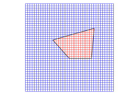
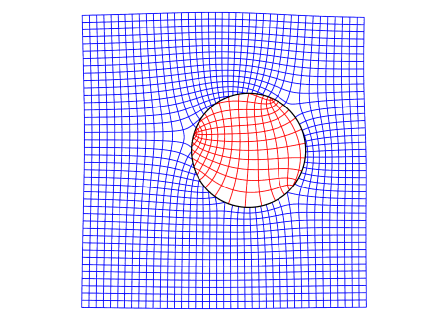
Figure 1. A coordinate grid (left) and its image under two conformal maps $\Phi_{1}$ and $\Phi_{2}$, defined in the exterior and in the interior of the polygonal quadrilateral of Example 4.8, resp. The exterior map $\Phi_{1}$ is normalized by assuming that $\Phi_{1}(z)=z+O(1/z)$ near infinity. The interior map $\Phi_{2}$ is normalized by assuming that $\Phi_{2}(\hat{\alpha})=0$ and $\Phi^{\prime}_{2}(\hat{\alpha})>0$ where $\hat{\alpha}$ is a given interior point to the quadrilateral.

3.2.

Computing the quadrilateral modulus. To compute the modulus $h={\rm Mod}(D;z_{1},z_{2},z_{3},z_{4})$, we first compute the unique conformal mapping $\Phi_{1}(z)$ from the unbounded domain $D$ onto the exterior of the unit disk with the normalization that $\Phi_{1}(z)=z+O(1/z)$ near infinity. This mapping function is computed by calling

$${\tt Phi1=plgcirmap(ver,inf)}$$

where ${\tt ver\{1\}=[z_{1},z_{2},z_{3},z_{4}]}$. Then, the conformal mapping

$$\hat{z}=\Phi(z)=\frac{1}{\Phi_{1}(z)}$$

maps the unbounded domain $D$ onto the unit disk ${\mathbb{D}}=\{\hat{z}\,:\,|\hat{z}|<1\}$. The boundary values $\hat{\eta}(t)=\Phi(\eta(t))$ form a parametrization of the unit circle $\partial{\mathbb{D}}$ and can be computed by calling

$$\mbox{\tt het = Phi1.zet}.$$

Hence, the vertices $z_{k}$, $k=1,2,3,4$, of the polygon domain $D$ are mapped onto the points $\hat{z}_{k}$, $k=1,2,3,4$, on the unit circle where

$$\hat{z}_{k}={\tt het((k-1)n/4+1)},\quad k=1,2,3,4.$$

Thus, by the conformal invariance of the modulus, the modulus of the quadrilateral $(D;z_{1},z_{2},z_{3},z_{4})$ is given by [HKV, NRRV, PS]

(3.3) $$h={\rm Mod}(D;z_{1},z_{2},z_{3},z_{4})={\rm Mod}({\mathbb{D}};\hat{z}_{1},\hat{z}_{2},\hat{z}_{3},\hat{z}_{4})=\frac{2}{\pi}\,\mu\left(1/\sqrt{k}\right)$$

where

(3.4) $$\mu(r)=\frac{\pi\,\mathchoice{\hbox{\,\fFt K}}{\hbox{\,\fFt K}}{\hbox{\,\fFa K}}{\hbox{\,\fFp K}}(r^{\prime})}{2\mathchoice{\hbox{\,\fFt K}}{\hbox{\,\fFt K}}{\hbox{\,\fFa K}}{\hbox{\,\fFp K}}(r)}\,,\quad k=|\hat{z}_{1},\hat{z}_{2},\hat{z}_{3},\hat{z}_{4}|=\frac{|\hat{z}_{1}-\hat{z}_{3}|\,|\hat{z}_{2}-\hat{z}_{4}|}{|\hat{z}_{1}-\hat{z}_{2}|\,|\hat{z}_{2}-\hat{z}_{4}|}\,.$$

3.5.

Computing the conformal mapping $f$ in (1.1). Here, we describe how the toolbox can be used to compute the conformal mapping $f$ from $D$ onto the rectangle $R=\{w\,:\,0<{\,\operatorname{Re}\,}w<1,\,0<{\,\operatorname{Im}\,}w<h\}$ in (1.1) that satisfies the condition (1.2). The method is summarized in Figure 2.

By the definition of $h={\rm Mod}({\mathbb{D}};\hat{z}_{1},\hat{z}_{2},\hat{z}_{3},\hat{z}_{4})$ [PS, p.52], there exists a conformal mapping

$$w=\Psi(\hat{z})$$

from the unit disk ${\mathbb{D}}$ onto the rectangle $R$ such that

$$\Psi(\hat{z}_{1})=0,\;\Psi(\hat{z}_{2})=1,\;\Psi(\hat{z}_{3})=1+\mathrm{i}h,\;\Psi(\hat{z}_{4})=\mathrm{i}h.$$

To compute such a conformal mapping $\Psi$, we first compute the unique conformal mapping

$$\tilde{z}=\Psi_{1}(w)$$

from the domain $R$ onto the unit disk ${\mathbb{D}}$ with the normalization

(3.6) $$\Psi_{1}(\hat{\alpha})=0,\quad\Psi_{1}^{\prime}(\hat{\alpha})>0$$

where $\hat{\alpha}$ is an auxiliary point in $R$, say $\hat{\alpha}=(1+\mathrm{i}h)/2$. This conformal mapping $\Psi_{1}$ can be computed by the MATLAB toolbox PlgCirMap by calling

$${\tt Psi1=plgcirmap(vers,halpha)}$$

where ${\tt vers\{1\}}=[0,1,1+\mathrm{i}h,\mathrm{i}h]$ is the vector of vertices of $\partial R$ and ${\tt halpha}=\hat{\alpha}$. The mapping function $\tilde{z}=\Psi_{1}(w)$ maps the vertices $0,1,1+\mathrm{i}h,\mathrm{i}h$ of $\partial R$ onto four points $\tilde{z}_{1},\tilde{z}_{2},\tilde{z}_{3},\tilde{z}_{4}\in\partial{\mathbb{D}}$ where

$$\tilde{z}_{k}={\tt tzet((k-1)n/4+1)},\quad k=1,2,3,4,$$

and tzet = Psi1.zet. These points are in general different from the points $\hat{z}_{1},\hat{z}_{2},\hat{z}_{3},\hat{z}_{4}$. Let

$$\hat{z}=\Psi_{2}(\tilde{z})=\hat{z}_{3}+\frac{(\hat{z}_{3}-\hat{z}_{1})(\hat{z}_{2}-\hat{z}_{3})(\tilde{z}_{2}-\tilde{z}_{1})(\tilde{z}-\tilde{z}_{3})}{(\hat{z}_{2}-\hat{z}_{1})(\tilde{z}_{2}-\tilde{z}_{3})(\tilde{z}-\tilde{z}_{1})-(\hat{z}_{2}-\hat{z}_{3})(\tilde{z}_{2}-\tilde{z}_{1})(\tilde{z}-\tilde{z}_{3})}\,,$$

then $\Psi_{2}$ maps the unit disk ${\mathbb{D}}$ onto itself such that $\Psi_{2}(\tilde{z}_{1})=\hat{z}_{1}$, $\Psi_{2}(\tilde{z}_{2})=\hat{z}_{2}$, and $\Psi_{2}(\tilde{z}_{3})=\hat{z}_{3}$. Thus, the function

$$w=(\Psi_{1}^{-1}\circ\Psi_{2}^{-1})(\hat{z})$$

maps the unit disk ${\mathbb{D}}$ onto the rectangle $R$ and takes the three points $\hat{z}_{1}$, $\hat{z}_{2}$, $\hat{z}_{3}$ to the three points $0$, $1$, $1+\mathrm{i}h$, respectively. Since the function $\Psi$ is also a conformal mapping from the unit disk ${\mathbb{D}}$ onto the rectangle $R$ and maps the three points $\hat{z}_{1},\hat{z}_{2},\hat{z}_{3}$ to the three points $0,1,1+\mathrm{i}h$, respectively, then we have

$$\Psi=\Psi_{1}^{-1}\circ\Psi_{2}^{-1}.$$

This is due to the fact of the uniqueness of the conformal mapping that maps the unit disk ${\mathbb{D}}$ onto the domain $R$ and maps three points on $\partial D$ to three points on $\partial R$ when $h$ is fixed.

Thus, the function

$$w=f(z)=(\Psi\circ\Phi)(z)=(\Psi_{1}^{-1}\circ\Psi_{2}^{-1}\circ\Phi)(z)$$

is the required unique conformal mapping satisfying (1.1) and (1.2).

Figure 2. The numerical computation of the conformal mapping $w=f(z)$ using the PlgCirMap MATLAB toolbox.

3.7.

Computing the values of the potential function $u$. Finally, we describe how to use the toolbox to compute the values of the mapping function $w=f(z)=\Psi_{1}^{-1}(\Psi_{2}^{-1}(\Phi(z)))$ and then the values of the potential function $u(z)$ for interior points $z\in D$.

First, for $z\in D$, the values of the mapping function $\hat{z}=\Phi(z)$ can be computed using the MATLAB function evalu from the PlgCirMap MATLAB toolbox by calling

$${\tt\hat{z}=1./evalu(Phi1,z,{{}^{\prime}d^{\prime}})}$$

For the Möbius transform, $\Psi_{2}^{-1}:{\mathbb{D}}\to{\mathbb{D}}$, it can be computed by the explicit formula

$$\tilde{z}=\Psi_{2}^{-1}(\hat{z})=\tilde{z}_{3}+\frac{(\tilde{z}_{3}-\tilde{z}_{1})(\tilde{z}_{2}-\tilde{z}_{3})(\hat{z}_{2}-\hat{z}_{1})(\hat{z}-\hat{z}_{3})}{(\tilde{z}_{2}-\tilde{z}_{1})(\hat{z}_{2}-\hat{z}_{3})(\hat{z}-\hat{z}_{1})-(\tilde{z}_{2}-\tilde{z}_{3})(\hat{z}_{2}-\hat{z}_{1})(\hat{z}-\hat{z}_{3})}\,.$$

Then, the values of the inverse mapping function $w=\Psi_{1}^{-1}(\tilde{z})$ can be computed by the MATLAB function evalu by calling

$${\tt w=evalu(Psi1,\tilde{z},{{}^{\prime}v^{\prime}})}$$

By computing the values of the function $w=f(z)$, we find the values of the potential function $u$ through

$$u(z)={\,\operatorname{Re}\,}f(z),\quad z\in D.$$

Since $\Phi(\infty)=0$, we have

$$u(\infty)={\,\operatorname{Re}\,}f(\infty)=\Psi_{1}^{-1}(\Psi_{2}^{-1}(\Phi(\infty)))=\Psi_{1}^{-1}(\Psi_{2}^{-1}(0)).$$

4. The main result and its proof

We will apply [NSV] to give a formula for the value of the potential function at infinity, $u(\infty),$ for a quadrilateral $Q=(D;z_{1},z_{2},z_{3},z_{4})$ in the case where $D$ is an unbounded domain with a boundary which is a convex polygonal line with vertices $z_{1}$, $z_{2}$, $z_{3}$, $z_{4}$, and interior angles of $D$ equal to

(4.1) $$(1-\alpha)\pi,\;(1-\beta)\pi,\;(1-\gamma)\pi,\;(1-\delta)\pi,\quad\alpha,\beta,\gamma,\delta\in(0,1),\quad\alpha+\beta+\gamma+\delta=2.$$

This formula for the potential function, given in Corollary 4.6, is our main result; it is expressed in terms of special functions.

Let $t=1/r^{2},$ where $r\in(0,1),$ be the unique root of the equation

(4.2) $$\text{Mod}(Q)={\mathchoice{\hbox{\,\fFt K}}{\hbox{\,\fFt K}}{\hbox{\,\fFa K}}{\hbox{\,\fFp K}}}(r^{\prime})/{\mathchoice{\hbox{\,\fFt K}}{\hbox{\,\fFt K}}{\hbox{\,\fFa K}}{\hbox{\,\fFp K}}}(r),\quad r^{\prime}=\sqrt{1-r^{2}};$$

here $\text{Mod}(Q)$ is the conformal modulus of $Q$. Denote $\mathcal{E}=\alpha+\beta+\gamma-1$,

$$\mathcal{A}=2(\mathcal{E}-1)^{2},\quad\mathcal{B}=(\mathcal{E}-1)[4-3(\alpha+\gamma)+(4-3(\alpha+\beta))t],$$

$$\mathcal{C}=2-3(\alpha+\gamma)+(\alpha+\gamma)^{2}+2(3-5\alpha-2\beta-2\gamma+2\alpha^{2}+2\alpha\beta+2\alpha\gamma+\beta\gamma)t$$

$$+(2-3(\alpha+\beta)+(\alpha+\beta)^{2})t^{2},\quad\mathcal{D}=(1-\alpha)(\alpha+\gamma-1+(\alpha+\beta-1)t)t,$$

$$\rho(x)=\frac{\alpha tx}{(1-\mathcal{E})x+\mathcal{E}(t+1)-\gamma t-\beta}\,.$$

In [NSV] the following result is actually proved.

Theorem 4.3.

The conformal mapping $f$ of the upper half plane onto $D$ is given by the generalized Schwarz-Christoffel formula [AF, Section 5.6, formula (5.6.3b)]

(4.4) $$f(z)=C\int_{0}^{z}\frac{\zeta^{\alpha}(\zeta-1)^{\beta}(\zeta-t)^{\gamma}}{(\zeta-z_{0})^{2}(\zeta-\overline{z}_{0})^{2}}\,d\zeta+z_{1},$$

$$C=(z_{2}-z_{1})\biggl{(}\int_{0}^{1}\frac{\zeta^{\alpha}(\zeta-1)^{\beta}(\zeta-t)^{\gamma}}{(\zeta-z_{0})^{2}(\zeta-\overline{z}_{0})^{2}}\,d\zeta\biggr{)}^{-1}.$$

Here $z_{0}=x_{0}+iy_{0}$ is a pole of $f$ satisfying the following equation:

(4.5) $$\frac{\alpha}{z_{0}}+\frac{\beta}{z_{0}-1}+\frac{\gamma}{z_{0}-t}=\frac{1}{\mathrm{i}y_{0}}\,.$$

The equation (4.5) has a unique solution $z_{0}$ in the upper half plane. Moreover, $x_{0}$ is the unique solution of the cubic equation

$$\mathcal{A}x^{3}+\mathcal{B}x^{2}+\mathcal{C}x+\mathcal{D}=0,$$

satisfying the inequality $x^{2}<\rho(x)$, and $y_{0}=\sqrt{\rho(x_{0})-x_{0}^{2}}$.

Now we will give a method to find $u(\infty)$ with the help of elliptic integrals of the first kind.

Let, as above, $D$ be an unbounded domain with boundary which is a convex polygonal line with vertices $z_{1}$, $z_{2}$, $z_{3}$, and $z_{4}$, and interior angles of $D$ satisfying (4.1). Let $r\in(0,1)$ be a unique solution of (4.2) and $t=1/r^{2}$.

Corollary 4.6.

For the unbounded polygonal quadrilateral $(D;z_{1},z_{2},z_{3},z_{4})$, the potential function (1.3) is equal to ${\,\operatorname{Re}\,}\psi\circ f^{-1}$ where $f$ is given by (4.4),

$$\psi(z)=\frac{F(r,\arcsin\sqrt{z})}{\mathchoice{\hbox{\,\fFt K}}{\hbox{\,\fFt K}}{\hbox{\,\fFa K}}{\hbox{\,\fFp K}}(r)}\,,$$

$F(r,\varphi)$ and $\mathchoice{\hbox{\,\fFt K}}{\hbox{\,\fFt K}}{\hbox{\,\fFa K}}{\hbox{\,\fFp K}}(r)$ are elliptic integrals given by (2.2) and (2.1). Moreover,

(4.7) $$u(\infty)={\,\operatorname{Re}\,}\,\psi(z_{0})$$

where $z_{0}$ is the unique root of (4.5) lying in the upper half plane.

Proof.

Actually, $\psi$ maps conformally the upper half plane onto the rectangle $[0,1]\times[0,h]$ and this immediately implies the statement of Corollary 4.6. ∎

4.8.

Some level sets of the exterior modulus. The polygon shown in Fig.3 has vertices $1,0,-19/25+\mathrm{i}\,21/25,28/25+\mathrm{i}\,69/50.$ Some level sets of the exterior modulus are shown, corresponding to values: $0.1$, $0.2$, $0.3$, $0.4$, $u(\infty)=0.471813...$, $0.6$, $0.7$, $0.8$ and $0.9$. Compare with [HRV2, Fig. 3.5 (b)].

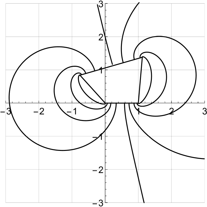
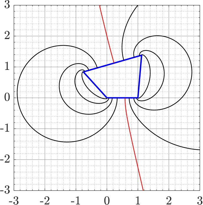
Figure 3. The exterior polygon 4.8 and the level curves of its potential function. The figure on the left/right side is produced with the Mathematica/MATLAB codes.

4.9.

Another example. The polygon shown in Fig.4 has vertices $1,0,-3/25+\mathrm{i}\,21/25,42/25+\mathrm{i}\,4$. The levels are: $0.1,0.2,u(\infty)=0.334052...,0.4,0.5,0.6,0.7,0.8$ and $0.9.$

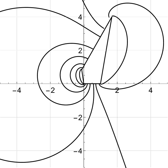
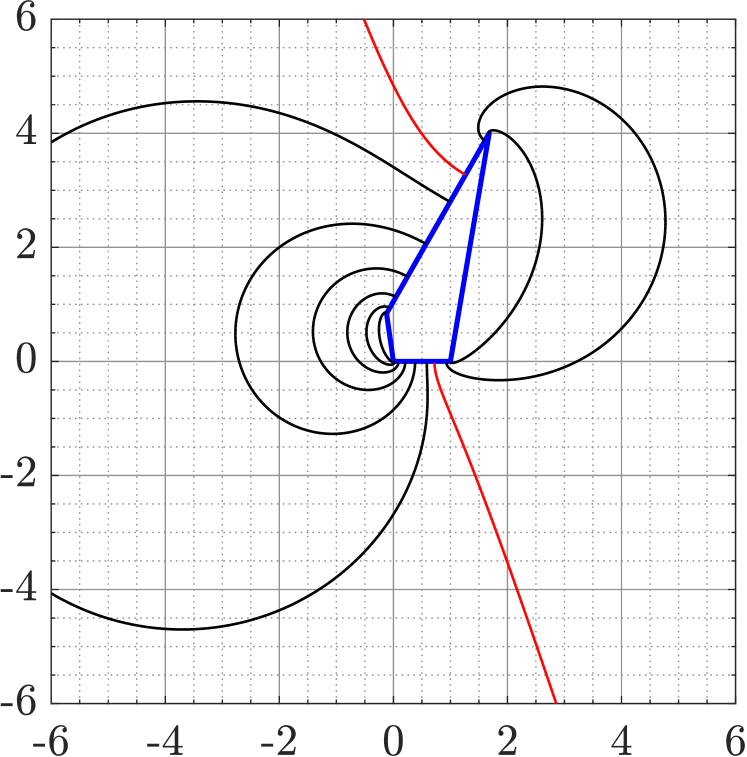
Figure 4. The exterior polygon 4.9 and the level curves of its potential function. The figure on the left/right side is produced with the Mathematica/MATLAB codes.

5. Exterior of the unit disk

We consider here the case of a circular quadrilateral determined by the unit disk and four points on the unit circle. Let $Q$ be the quadrilateral which is the exterior of the unit disk with vertices $e^{\mathrm{i}\beta}$, $e^{\mathrm{i}\alpha}$, $e^{-\mathrm{i}\alpha}$, $e^{-\mathrm{i}\beta}$, $0<\alpha<\beta<\pi$. The Möbius transformation

$$w=T(z)=\frac{z-a}{1-az},\quad a=\frac{1-\sqrt{\tan\frac{\alpha}{2}\tan\frac{\beta}{2}}}{1+\sqrt{\tan\frac{\alpha}{2}\tan\frac{\beta}{2}}}\,,$$

maps it onto the quadrilateral $Q_{1}$ which is the exterior of the unit disk with vertices $-e^{-\mathrm{i}\gamma}$, $e^{\mathrm{i}\gamma}$, $e^{-\mathrm{i}\gamma}$, $-e^{-\mathrm{i}\gamma}$, where

$$\cos\gamma=\frac{\sin\frac{\beta-\alpha}{2}}{\sin\frac{\beta+\alpha}{2}}\,,\quad 0<\gamma<\pi/2.$$

The Möbius transformation

$$\omega=S(w)=\frac{1}{\sqrt{\lambda}}\,\frac{w-\mathrm{i}}{1-\mathrm{i}w}$$

maps $Q_{1}$ onto the quadrilateral $Q_{2}$ which is the upper half plane with vertices $-1/\lambda$, $-1$, $1$, $1/\lambda$, where

$$\lambda=1+2\tan^{2}\gamma-2\tan\gamma\sqrt{1+\tan^{2}\gamma}.$$

At last,

$$\zeta=g(\omega)=\frac{F(\lambda,\arcsin\omega)}{2\mathchoice{\hbox{\,\fFt K}}{\hbox{\,\fFt K}}{\hbox{\,\fFa K}}{\hbox{\,\fFp K}}(\lambda)}\,+0.5$$

maps $Q_{2}$ onto $Q_{3}$ which is the rectangle $[0,1]\times[0,h]$ with vertices $0$, $1$, $1+\mathrm{i}h$, $\mathrm{i}h$, where $h$ is the conformal modulus of $Q$.

The function

$$u(z)={\,\operatorname{Re}\,}g\circ S\circ T(z)$$

is the potential function for $Q$. We note that $g\circ S\circ T(\infty)=g\circ S(-1/a)=g\left(-\frac{1}{\sqrt{\lambda}}\,\frac{1+\mathrm{i}a}{a+\mathrm{i}}\right)$, therefore, for $u_{0}=u(\infty)$ we have

$$u_{0}={\,\operatorname{Re}\,}g\left(-\frac{1}{\sqrt{\lambda}}\,\frac{1+\mathrm{i}a}{a+\mathrm{i}}\right).$$

If we put $u_{0}=u(\infty)$, then the parametric representation of the level curve $u=u_{0}$ takes the form

$$z=T^{-1}\circ S^{-1}\circ\,\mathrm{sn}((2u_{0}-1)\mathchoice{\hbox{\,\fFt K}}{\hbox{\,\fFt K}}{\hbox{\,\fFa K}}{\hbox{\,\fFp K}}(\lambda)+\mathrm{i}\xi,\lambda),\quad 0\leq\xi\leq\mathchoice{\hbox{\,\fFt K}}{\hbox{\,\fFt K}}{\hbox{\,\fFa K}}{\hbox{\,\fFp K}}^{\prime}(\lambda).$$

or

$$z=\frac{\sqrt{\lambda}(a-\mathrm{i})\,\mathrm{sn}((2u_{0}-1)\mathchoice{\hbox{\,\fFt K}}{\hbox{\,\fFt K}}{\hbox{\,\fFa K}}{\hbox{\,\fFp K}}(\lambda)+\mathrm{i}\xi,\lambda)+(1-\mathrm{i}a)}{\sqrt{\lambda}(1-\mathrm{i}a)\,\mathrm{sn}((2u_{0}-1)\mathchoice{\hbox{\,\fFt K}}{\hbox{\,\fFt K}}{\hbox{\,\fFa K}}{\hbox{\,\fFp K}}(\lambda)+i\xi,\lambda)+(a-\mathrm{i})}\,,\quad 0\leq\xi\leq\mathchoice{\hbox{\,\fFt K}}{\hbox{\,\fFt K}}{\hbox{\,\fFa K}}{\hbox{\,\fFp K}}^{\prime}(\lambda).$$

Here $\mathrm{sn}(\,\cdot\,,\lambda)$  is the Jacobi sine.

The level curve $\{u=u_{0}\}$ is symmetric with respect to the real axis. If we consider its upper half, then, as numerical calculations show, we can see that it is very close to a (rectilinear) ray and is essentially distinct from it only in a small neighborhood of its endpoint lying on the unit circle.

Figure 5. The level curves of the potential function for the mixed Dirichlet-Neumann problem corresponding to the levels $0.2j\cdot u_{0}$, $1\leq j\leq 5$; $u_{0}+0.2k(1-u_{0})$, $1\leq k\leq 4$; $\alpha=0.5$, $\beta=1.7$. The quadrilateral is the exterior of the unit disk and its vertices are indicated by the endpoints of the radii.

The Fig.5 was produced by the following Mathematica script.

alpha = 0.5; beta = 1.7; a = (1 - Sqrt[Tan[alpha/2]Tan[beta/2]])/
(1 + Sqrt[Tan[alpha/2] Tan[beta/2]]);
gamma = ArcCos[Sin[(beta - alpha)/2]/Sin[(beta + alpha)/2]];
lambda = 1 + 2 (Tan[gamma])^2 - 2*Tan[gamma]* Sqrt[1 + (Tan[gamma])^2];
zeta0 = (-1/Sqrt[lambda]) (1 + I*a)/(a + I);
u0 = Re[EllipticF[ArcSin[zeta0], lambda^2]/(2*EllipticK[lambda^2])] + 0.5;
u1 = 0.2*u0; u2 = 0.4*u0; u3 = 0.6*u0; u4 = 0.8*u0; u5 = u0 + 0.2 (1 - u0);
u6 = u0 + 0.4 (1 - u0); u7 = u0 + 0.6 (1 - u0); u8 = u0 + 0.8 (1 - u0);
t0 = EllipticK[1 - lambda^2]/EllipticK[lambda^2];
H[xi_, u_] = (Sqrt[lambda] (a - I) JacobiSN[(2*u - 1 + I*xi) (EllipticK[lambda^2]),
lambda^2] + (1 - a*I))/(Sqrt[lambda] (1 - a*I) JacobiSN[(2*u - 1 + I*xi)
(EllipticK[lambda^2]), lambda^2] + (a - I));
figInf3 = ParametricPlot[{{Re[H[t, u0]],Im[H[t, u0]]}, {Re[H[t, u1]], Im[H[t, u1]]},
{Re[H[t, u2]],Im[H[t, u2]]}, {Re[H[t, u3]], Im[H[t, u3]]}, {Re[H[t, u4]],
Im[H[t, u4]]}, {Re[H[t, u5]], Im[H[t, u5]]}, {Re[H[t, u6]],Im[H[t, u6]]},
{Re[H[t, u7]], Im[H[t, u7]]}, {Re[H[t, u8]],Im[H[t, u8]]}, {Cos[2*Pi*t/t0],
Sin[2*Pi*t/t0]}, {(t/t0) Cos[alpha], (t/t0) Sin[alpha]}, {(t/t0) Cos[beta],
(t/t0) Sin[beta]}, {(t/t0) Cos[alpha], -(t/t0) Sin[alpha]}, {(t/t0) Cos[beta],
-(t/t0) Sin[beta]}}, {t, 0, t0}, PlotRange -> 2.8, PlotStyle -> Black,
AxesStyle -> Black]

The radii in the figure show the location of the vertices of the quadrilateral.

6. Some numerical results

Now we will give values of $u(\infty)$ for some unbounded polygonal quadrilaterals

$$Q=(D;z_{1},z_{2},z_{3},z_{4})$$

with vertices $z_{1}=1$, $z_{2}=0$, $z_{3}=B$, $z_{4}=A$ and angles $\pi(1+\alpha_{k})$, $1\leq k\leq 4$. To calculate $u(\infty)$, we use the Mathematica module ExtMod[$B,A,n,wp$] from [NSV, Appendix A] written with the help of the Wolfram Mathematica system. This function returns the values of $\text{Mod}(Q)$, $\alpha_{1}$, $\alpha_{2}$, $\alpha_{3}$, $\alpha_{4}$, $t$, and $z_{0}$. For example, if $A=7+5\,\mathrm{i}$, $B=-1+2\,\mathrm{i}$ (see Table 1, Line 2), then we use the module ExtMod[$B,A,n,wp$] as follows:

uInfty[A_, B_] := Module[{v = ExtMod[B,A,2,16], r, t, z0}, t = v[[6]]; z0 = v[[7]];
r = 1/Sqrt[t]; Re[EllipticF[ArcSin[Sqrt[z0]], r^2]/EllipticK[r^2]]];
DecimalForm[uInfty[7 + 5 I,-1 + 2 I ],16]

In the above codelines we have used the notation of (4.7), to make the application of
ExtMod[$B,A,n,wp$] transparent for the readers. Here the parameter $wp$ stands for the accuracy goal, and the above call ExtMod[B,A,2,16] means that the desired accuracy is $10^{-16}.$

Table 1. The values of $u(\infty)$ for some polygonal quadrilaterals computed using the formula (4.7) and using the PlgCirMap MATLAB toolbox [N]. The computed values agree with $9$ decimal places or more.

$A$	$B$	Using the Formula (4.7)	PlgCirMap toolbox method
7 + 5 I	$-1+2$ I	0.3782951219491777	0.378295121963035
8 + 3 I	$-1$ + I	0.3507184214435048	0.350718421549051
5 + 5 I	$-3$ + I	0.4209495357540314	0.420949535761708
7 + 4 I	$-3$ + 3 I	0.4473431220217027	0.447343122027837
5 + 5 I	$-1$ + 2 I	0.3916188047098933	0.391618804701488
7 + 5 I	I	0.3172197705784933	0.317219770131948
7 + 3 I	1 + 2 I	0.3917841755037506	0.391784175504020
4 + 5 I	$-2$ + I	0.3960930352825737	0.396093035293408
1 + I	I	0.5000000000000000	0.500000000000000

References

- [AF] M. J. Ablowitz and A.S. Fokas, Complex variables: introduction and applications. Second edition. Cambridge Texts in Applied Mathematics. Cambridge University Press, Cambridge, 2003. xii+647 pp.
- [A] L.V. Ahlfors, Conformal Invariants: Topics in Geometric Function Theory, vol. 371, American Mathematical Soc., 2010.
- [Ak] N. I. Akhiezer, Elements of the Theory of Elliptic Functions. Transl. of Mathematical Monographs, vol. 79, American Mathematical Soc., RI, 1990.
- [AVV] G. D. Anderson, M. K. Vamanamurthy, and M. Vuorinen, Conformal invariants, inequalities and quasiconformal maps. Canadian Mathematical Society Series of Monographs and Advanced Texts. A Wiley-Interscience Publication. J. Wiley, 1997.
- [B] H. Bateman and A. Erdelyi, Higher transcendental functions. Vol. 1, 1953.
- [DT] T. A. Driscoll and L. N. Trefethen, Schwarz-Christoffel mapping. Cambridge Monographs on Applied and Computational Mathematics, 8. Cambridge University Press, Cambridge, 2002. xvi+132 pp.
- [D] V. N. Dubinin, Condenser capacities and symmetrization in geometric function theory. Translated from the Russian by Nikolai G. Kruzhilin. Springer, Basel, 2014, xii+344 pp.
- [GM] J. B. Garnett and D. E. Marshall, Harmonic measure. Reprint of the 2005 original. New Mathematical Monographs, 2. Cambridge University Press, Cambridge, 2008, xvi+571 pp. ISBN: 978-0-521-72060-1.
- [GOL] G. M. Goluzin, Geometric theory of functions of a complex variable. Translations of Mathematical Monographs, Vol. 26 American Mathematical Society, Providence, R.I. 1969 vi+676 pp.
- [HRV1] H. Hakula, A. Rasila, and M. Vuorinen, On moduli of rings and quadrilaterals: algorithms and experiments. SIAM J. Sci. Comput. 33 (2011), no. 1, 279–302.
- [HRV2] H. Hakula, A. Rasila, and M. Vuorinen, Computation of exterior moduli of quadrilaterals. Electron. Trans. Numer. Anal. 40 (2013), 436–451.
- [HKV] P. Hariri, R. Klén, and M. Vuorinen, Conformally Invariant Metrics and Quasiconformal Mappings, Springer Monographs in Mathematics, Springer, Berlin, 2020.
- [HVV] V. Heikkala, M. K. Vamanamurthy, and M. Vuorinen, Generalized elliptic integrals. Comput. Methods Funct. Theory 9 (2009), no. 1, 75–109.
- [KY] P. K. Kythe, Handbook of conformal mappings and applications. CRC Press, Boca Raton, FL, 2019. xxxv+906 pp.
- [LSN] J. Liesen, O. Séte, and M.M.S. Nasser, Fast and accurate computation of the logarithmic capacity of compact sets. Comput. Methods Funct. Theory 17 (2017), no. 4, 689–713.
- [N] M.M.S. Nasser, PlgCirMap: A MATLAB toolbox for computing conformal mappings from polygonal multiply connected domains onto circular domains. SoftwareX 11 (2020), 100464.
- [NRRV] M. Nasser, O. Rainio, A. Rasila, M. Vuorinen, T. Wallace, H. Yu, and X. Zhang, Circular arc polygons, numerical conformal mappings, and moduli of quadrilaterals. arXiv 2107.11485.
- [NRV] M. M.S. Nasser, O. Rainio, and M. Vuorinen, Condenser capacity and hyperbolic perimeter. Comput. Math. Appl. 105(2022), 54–74. arXiv:2103.10237 [math.NA].
- [NV] M. M.S. Nasser and M. Vuorinen, Conformal invariants in simply connected domains. Comput. Methods Funct. Theory 20 (2020), 747–775.
- [NSV] S. Nasyrov, T. Sugawa, and M. Vuorinen, Moduli of quadrilaterals and quasiconformal reflection. arXiv:2111.08304.
- [PS] N. Papamichael and N. Stylianopoulos, Numerical conformal mapping: domain decomposition and the mapping of quadrilaterals, World Scientific, Singapore; Hackensack, N.J., 2010.
- [WK] M. Wala and A. Klockner, Conformal mapping via a density correspondence for the double-layer potential. SIAM J. Sci. Comput. 40 (2018), A3715–A3732.
- [W] R. Wegmann, Methods for numerical conformal mapping, Handbook of Complex Analysis: Geometric Function Theory, Vol. 2, ed. by R. Kühnau, Elsevier B. V., 351–477, 2005.