Realization of the inverse scattering transform method for the Korteweg–de Vries equation

Abstract

A method for practical realization of the inverse scattering transform method for the Korteweg–de Vries equation is proposed. It is based on analytical representations for Jost solutions and for integral kernels of transformation operators obtained recently ([22], [23]). The representations have the form of functional series in which the first coefficient plays a crucial role both in solving the direct scattering and the inverse scattering problems. The direct scattering problem reduces to computation of a number of the coefficients following a simple recurrent integration procedure with a posterior calculation of scattering data  by well known formulas. The inverse scattering problem reduces to a system of linear algebraic equations from which the first component of the solution vector leads to the recovery of the potential. We prove the applicability of the finite section method to the system of linear algebraic equations and discuss numerical aspects of the proposed method. Numerical examples are given, which reveal the accuracy and speed of the method.

1 Introduction

The inverse scattering transform method (ISTM) for solving nonlinear partial differential equations was discovered in 1967 in the paper [16] in application to the Korteweg–de Vries (KdV) equation, which can be written in the form

$$u_{t}-6uu_{x}+u_{xxx}=0.$$

The equation models shallow water waves and admits solitary wave solutions.

The method was further developed in 1972 in [37] in application to another important equation of mathematical physics, the nonlinear Schrödinger equation, whose principal applications are to the propagation of light in nonlinear optical fibers (see, e.g., [34]).

After those first works the ISTM encountered many other applications related to a large number of nonlinear evolution partial differential equations of mathematical physics. We refer to the books [1], [2], [3] covering parts of this wide topic.

In theory the ISTM offers a beautiful way for solving the initial value problem for the nonlinear equation. In order to obtain the solution at a given time one has to solve successively a couple of spectral problems for a linear ordinary differential equation (or system): a direct and an inverse scattering problems. If one is interested in visualizing the evolution of the solution in time, then not just one but a number of inverse scattering problems has to be solved.

The most important practical result of the ISTM until now is the possibility to obtain solitonic solutions (see, e.g., [1], [2], [3], [10], [27], [29]). However, the ISTM is not widely used for numerical solution of the initial value problems with general initial profiles (not necessarily leading to solitonic solutions). The reason is the difficulty of solving the direct and inverse scattering problems on the line. Instead of the ISTM many purely numerical approaches have been developed for solving nonlinear evolutionary equations, in particular, the KdV equation (see, e.g., [5], [6], [12], [13], [32]). They have important limitations. (a) Instead of considering problems on the whole line with respect to the space variable, they solve problems on finite intervals with some fictitious boundary conditions, and thus, in general, do not serve for solving the initial value problem on the whole line. (b) In order to obtain a picture of the solution at a given time the solution needs to be computed for preceding times on a sufficiently fine mesh.

Recently, with the aid of several new ideas developed and implemented, there appeared a feasible way for practical realization of the ISTM in all its might and with all attractive features. This is the main subject of the present work.

It is well known that in principle solution of direct and inverse scattering problems on the line for the one-dimensional Schrödinger equation

$$-y^{\prime\prime}+q(x)y=\rho^{2}y,\quad-\infty<x<\infty$$

with $(1+\left|x\right|)q(x)\in L_{1}(-\infty,\infty)$, and $\rho\in\mathbb{C}$, reduces to construction of the kernel of an appropriate transmutation (transformation) operator, which maps the exponential function into the Jost solution. When solving the direct problem, the knowledge of the transmutation kernel implies the knowledge of the Jost solution for all values of the spectral parameter, which in turn leads to the possibility of computing scattering data. And solution of the inverse problem reduces to the Gelfand-Levitan-Marchenko integral equation serving for calculation of the transmutation kernel from given scattering data. The potential is recovered from the transmutation kernel by one differentiation.

However, until recently the approach based on the transmutation kernel for solving both direct and inverse scattering problems in general has not resulted in an efficient numerical method. Construction of the transmutation kernel by a known potential is quite a challenge as well as the recovery of the transmutation kernel from the Gelfand-Levitan-Marchenko equation.

In the recent work [22], [23], [14] it was shown that solution of both direct and inverse scattering problems can be reduced to calculation of the first coefficient of a Fourier-Laguerre series expansion of the transmutation kernel. The kernel itself is not needed. To the difference from the transmutation kernel which is a function of two independent variables, the first coefficient is a function of one variable. Its knowledge allows one to compute the Jost solution for all values of the spectral parameter (which serves for solving the direct problem), as well as to recover the potential (when solving the inverse problem). More precisely, it is convenient to consider simultaneously two Jost solutions, which we denote by $e(\rho,x)$ and $g(\rho,x)$, satisfying corresponding asymptotic conditions at the “$+$” and “$-$” infinities, respectively, as well as the first coefficients of Fourier-Laguerre series expansions of two corresponding transmutation kernels. The first coefficients we denote by $a_{0}(x)$ and $b_{0}(x)$, respectively. They can be written in terms of the Jost solutions as follows

$$a_{0}(x)=e(\frac{i}{2},x)e^{\frac{x}{2}}-1$$ (1.1)

and

$$b_{0}(x)=g(\frac{i}{2},x)e^{-\frac{x}{2}}-1.$$ (1.2)

Thus, to know $a_{0}(x)$ is equivalent to know the Jost solution $e(\rho,x)$ for $\rho=\frac{i}{2}$ and similarly, to know $b_{0}(x)$ is equivalent to know the Jost solution $g(\rho,x)$ for $\rho=\frac{i}{2}$. It is obvious that the knowledge of $a_{0}(x)$ or $b_{0}(x)$ is sufficient for recovering $q$. Indeed, from (1.1) and (1.2) it follows that

$$q=\frac{a_{0}^{\prime\prime}-a_{0}^{\prime}}{a_{0}+1}$$ (1.3)

and

$$q=\frac{b_{0}^{\prime\prime}+b_{0}^{\prime}}{b_{0}+1}.$$ (1.4)

Moreover, in [22], [23] a system of linear algebraic equations was derived for the coefficients of the Fourier-Laguerre series of the transmutation kernel and thus $a_{0}(x)$ and $b_{0}(x)$ can be obtained by solving the corresponding system of linear algebraic equations.

Furthermore, as it was shown in [14] (see also [23, Chapter 10]) the Jost solution $e(\rho,x)$ for all values of $\rho$, $\operatorname{Im}\rho\geq 0$ can be quite easily obtained from $a_{0}(x)$, and similarly $g(\rho,x)$ from $b_{0}(x)$. Calculation of the Jost solutions from $a_{0}(x)$ and $b_{0}(x)$ reduces to a recurrent integration procedure [14], [23, Chapter 10], which eventually leads to a very convenient procedure for computing both the discrete scattering data and the reflection coefficients by evaluating power series in a unitary disk of the complex variable $z:=\left(\frac{1}{2}+i\rho\right)/\left(\frac{1}{2}-i\rho\right)$. The overall approach based on the computation of the functions $a_{0}(x)$ and $b_{0}(x)$ for solving both the direct and inverse scattering problems leads to a direct, quite simple and efficient numerical method for solving the Cauchy problem for the KdV equation. In the present work we discuss this method in detail.

We provide a rigorous justification of the method which includes the applicability of the finite section method, the analysis of the convergence rate in dependence on the smoothness of the potential, the existence of the derivatives $a_{0}^{\prime}$, $a_{0}^{\prime\prime}$ and $b_{0}^{\prime}$, $b_{0}^{\prime\prime}$ (when $a_{0}$ and $b_{0}$ are computed as solutions of the linear algebraic systems), which is required for recovering the potential $q$ from (1.3) or (1.4), respectively, and discuss details of its numerical implementation. Numerical examples are given, which reveal the accuracy and speed of the method proposed.

2 Representations for Jost solutions and their derivatives

We consider the classical one-dimensional scattering problem. Given a real valued function $q(x)$, $-\infty<x<\infty$ satisfying the condition

$$\int_{-\infty}^{\infty}\left(1+\left|x\right|\right)\left|q(x)\right|dx<\infty,$$ (2.1)

compute the corresponding scattering data which include a finite set of eigenvalues and norming constants and a reflection coefficient. All the scattering data are defined in terms of so-called Jost solutions of the Schrödinger equation

$$-y^{\prime\prime}+q(x)y=\lambda y,\quad-\infty<x<\infty$$ (2.2)

where $\lambda\in\mathbb{C}$ is a spectral parameter, $\lambda=\rho^{2}$, $\rho\in\overline{\Omega}_{+}:=\left\{\rho\in\mathbb{C}\mid\operatorname{Im}\rho\geq 0\right\}$. They are the unique solutions $e(\rho,x)$ and $g(\rho,x)$ of (2.2) satisfying the asymptotic relations

$$e(\rho,x)=e^{i\rho x}\left(1+o(1)\right),\quad e^{\prime}(\rho,x)=i\rho e^{i\rho x}\left(1+o(1)\right),\quad x\rightarrow\infty,$$ (2.3)

$$g(\rho,x)=e^{-i\rho x}\left(1+o(1)\right),\quad g^{\prime}(\rho,x)=-i\rho e^{-i\rho x}\left(1+o(1)\right),\quad x\rightarrow-\infty$$

uniformly in $\overline{\Omega}_{+}$. When $\rho\in\mathbb{R}$ we have

$$e(-\rho,x)=\overline{e(\rho,x)},\quad g(-\rho,x)=\overline{g(\rho,x)}.$$ (2.4)

Under the condition (2.1) the Jost solutions admit the following integral representations

$$e(\rho,x)=e^{i\rho x}+\int_{x}^{\infty}A(x,t)e^{i\rho t}dt$$ (2.5)

and

$$g(\rho,x)=e^{-i\rho x}+\int_{-\infty}^{x}B(x,t)e^{-i\rho t}dt$$ (2.6)

where $A$ and $B$ are real valued functions such that

$$A(x,x)=\frac{1}{2}\int_{x}^{\infty}q(t)dt,$$ (2.7)

$$B(x,x)=\frac{1}{2}\int_{-\infty}^{x}q(t)dt,$$

$A(x,\cdot)\in L_{2}\left(x,\infty\right)$ and $B(x,\cdot)\in L_{2}\left(-\infty,x\right)$. More on the properties of the kernels $A$ and $B$ can be found in [28].

Theorem 2.1.

[22], [23] The functions $A$ and $B$ admit the following series representations

$$A(x,t)=\sum_{n=0}^{\infty}a_{n}(x)L_{n}(t-x)e^{\frac{x-t}{2}}$$ (2.8)

and

$$B(x,t)=\sum_{n=0}^{\infty}b_{n}(x)L_{n}(x-t)e^{-\frac{x-t}{2}}$$ (2.9)

where $L_{n}$ stands for the Laguerre polynomial of order $n$.

For any $x\in\mathbb{R}$ fixed, the series converge in the norm of $L_{2}\left(x,\infty\right)$ and $L_{2}\left(-\infty,x\right)$, respectively.

For the coefficients $a_{0}(x)$ and $b_{0}(x)$ the equalities are valid

$$a_{0}(x)=e(\frac{i}{2},x)e^{\frac{x}{2}}-1$$ (2.10)

and

$$b_{0}(x)=g(\frac{i}{2},x)e^{-\frac{x}{2}}-1.$$ (2.11)

The coefficients $a_{n}(x)$, $b_{n}(x)$, $n=0,1,\ldots$ are the unique solutions of the equations

$$La_{0}-a_{0}^{\prime}=q,$$ (2.12)

$$Lb_{0}+b_{0}^{\prime}=q,$$ (2.13)

$$La_{n}-a_{n}^{\prime}=La_{n-1}+a_{n-1}^{\prime},\quad n=1,2,\ldots,$$

$$Lb_{n}+b_{n}^{\prime}=Lb_{n-1}-b_{n-1}^{\prime},\quad n=1,2,\ldots,$$

with $L:=\frac{d^{2}}{dx^{2}}-q(x)$, satisfying the boundary conditions $a_{n}(x)=o(1)$, when $x\rightarrow+\infty$ and $b_{n}(x)=o(1)$, when $x\rightarrow-\infty$.

In [14] (see also [23]) a recurrent integration procedure for efficient computation of the coefficients of the series (2.8) and (2.9) was derived. We give it in Appendix.

Note that due to the identity $L_{n}(0)=1$, for all $n=0,1,\ldots$, from (2.8) and (2.9) two useful relations follow

$$\sum_{n=0}^{\infty}a_{n}(x)=A(x,x)=\frac{1}{2}\int_{x}^{\infty}q(t)dt,\quad\sum_{n=0}^{\infty}b_{n}(x)=B(x,x)=\frac{1}{2}\int_{-\infty}^{x}q(t)dt.$$

Denote

$$z:=\frac{\frac{1}{2}+i\rho}{\frac{1}{2}-i\rho}.$$ (2.14)

Notice that this is a Möbius transformation of the upper halfplane of the complex variable $\rho$ onto the unit disc $D=\left\{z\in\mathbb{C}:\,\left|z\right|\leq 1\right\}$. In terms of the parameter $z$ the following representations for the Jost solutions were obtained in [22] (see also [15] and [23])

$$e(\rho,x)=e^{i\rho x}\left(1+\left(z+1\right)\sum_{n=0}^{\infty}\left(-1\right)^{n}z^{n}a_{n}(x)\right)$$ (2.15)

and

$$g(\rho,x)=e^{-i\rho x}\left(1+\left(z+1\right)\sum_{n=0}^{\infty}\left(-1\right)^{n}z^{n}b_{n}(x)\right)$$ (2.16)

where the coefficients $a_{n}$ and $b_{n}$ can be constructed following the recurrent integration procedure described in Appendix.

The coefficients $a_{n}$ and $b_{n}$ are real valued functions, $a_{n}(x)\rightarrow 0$ when $x\rightarrow+\infty$ while $b_{n}(x)\rightarrow 0$ when $x\rightarrow-\infty$. For any $x\in\mathbb{R}$ the series $\sum_{n=0}^{\infty}a_{n}^{2}(x)$ and $\sum_{n=0}^{\infty}b_{n}^{2}(x)$ converge, which is a consequence of the fact that they are Fourier coefficients with respect to the system of Laguerre polynomials of corresponding functions from $L_{2}\left(0,\infty;e^{-t}\right)$ (see [15]). Hence for any $x\in\mathbb{R}$ the functions $e(\rho,x)e^{-i\rho x}-1$ and $g(\rho,x)e^{i\rho x}-1$ belong to the Hardy space $H^{2}(D)$ as functions of $z$ (this is due to the well known result from complex analysis, see, e.g., [33, Theorem 17.12]).

Analogous representations were obtained for the derivatives with respect to $x$ of the Jost solutions under an additional assumption of the absolute continuity of the potential $q$ (see [15]),

$$e^{\prime}(\rho,x)=e^{i\rho x}\left(\frac{z-1}{2(z+1)}-\frac{1}{2}\int_{x}^{\infty}q(t)dt+(z+1)\sum_{n=0}^{\infty}\left(-1\right)^{n}z^{n}d_{n}(x)\right)$$ (2.17)

$$g^{\prime}(\rho,x)=e^{-i\rho x}\left(-\frac{z-1}{2(z+1)}+\frac{1}{2}\int_{-\infty}^{x}q(t)dt+(z+1)\sum_{n=0}^{\infty}\left(-1\right)^{n}z^{n}c_{n}(x)\right)$$ (2.18)

where the coefficients $\left\{d_{n}\right\}$ and $\left\{c_{n}\right\}$ are obtained from the coefficients $\left\{a_{n}\right\}$ and $\left\{b_{n}\right\}$, respectively, with the aid of the relations given in Appendix. Here we emphasize that the whole procedure of computation of the four sets of coefficients requires the computation of the Jost solutions $e(\frac{i}{2},x)$, $g(\frac{i}{2},x)$ and their first derivatives. All subsequent operations besides arithmetic operations involve the integration only, which from a practical viewpoint makes the procedure convenient for efficient computation. For the representations (2.15)-(2.18) truncation error estimates were obtained in [15].

Remark 2.2.

From (2.10) and (2.11) it follows that the knowledge of $a_{0}$ or $b_{0}$ is sufficient for recovering $q$. Namely,

$$q=\frac{a_{0}^{\prime\prime}-a_{0}^{\prime}}{a_{0}+1}$$ (2.19)

and

$$q=\frac{b_{0}^{\prime\prime}+b_{0}^{\prime}}{b_{0}+1}.$$ (2.20)

Indeed, from (2.10) we have that $e(\frac{i}{2},x)=e^{-\frac{x}{2}}\left(a_{0}(x)+1\right)$. Differentiating twice this equality and recalling that $e(\frac{i}{2},x)$ is a solution of the equation $-y^{\prime\prime}+q(x)y=-\frac{1}{4}y$ gives us (2.19). The equality (2.20) is obtained analogously.

3 Scattering data

We refer to the books [10, 28, 29, 36] for the theory of the scattering problem. Here we introduce only the definitions indispensable for the present work.

Consider the following scattering amplitudes (elements of the scattering matrix) $a(\rho)=-\frac{1}{2i\rho}W\left[e(\rho,x),g(\rho,x)\right]$ and $b(\rho)=\frac{1}{2i\rho}W\left[e(\rho,x),g(-\rho,x)\right]$, $\rho\in\mathbb{R}$ where $W$ denotes the Wronskian. Notice that since the Wronskian of any pair of solutions of (2.2) is constant, we may consider it at $x=0$. Thus,

$$a(\rho)=-\frac{1}{2i\rho}W\left[e(\rho,0),g(\rho,0)\right]\quad\rho\in\overline{\Omega_{+}},$$

and

$$b(\rho)=\frac{1}{2i\rho}W\left[e(\rho,0),g(-\rho,0)\right],\quad\rho\in\mathbb{R}.$$

Notice that the second expression is well defined for real values of $\rho$ only, because when $\operatorname{Im}\rho>0$, a solution of (2.2) behaving like $e^{-i\rho x}$ when $x\rightarrow-\infty$ is not unique.

The reflection coefficients (right (+) and left (-)) have the form [36, p. 210]

$$s^{\pm}(\rho):=\mp\frac{b(\mp\rho)}{a(\rho)},\quad\rho\in\mathbb{R}.$$ (3.1)

We recall that the eigenvalues of (2.2), if they exist, form a finite set of negative numbers $\lambda_{k}=\rho_{k}^{2}=\left(i\tau_{k}\right)^{2}$, $0<\tau_{1}<\ldots<\tau_{N}$. The corresponding norming constants are introduced as follows

$$\alpha_{k}^{+}:=\left(\int_{-\infty}^{\infty}e^{2}(\rho_{k},x)dx\right)^{-1}\quad\text{and\quad}\alpha_{k}^{-}:=\left(\int_{-\infty}^{\infty}g^{2}(\rho_{k},x)dx\right)^{-1}.$$

For their computation another formula can be used [36, p. 215]

$$\alpha_{k}^{\pm}=\frac{\left(d_{k}\right)^{\pm 1}}{ia^{\prime}(\rho_{k})}$$ (3.2)

where the constants $d_{k}$ are defined from the relation $d_{k}=g(\rho_{k},x)/e(\rho_{k},x)=g(\rho_{k},0)/e(\rho_{k},0)$ (notice that when $\lambda_{k}=\rho_{k}^{2}$ is an eigenvalue, the Jost solutions $e(\rho_{k},x)$ and $g(\rho_{k},x)$ are necessarily linearly dependent).

The sets

$$J^{\pm}=\left\{s^{\pm}(\rho),\,\rho\in\mathbf{R};\,\lambda_{k},\,\alpha_{k}^{\pm},\,k=\overline{1,N}\right\}$$

are called the right and left scattering data, respectively.

To solve the direct scattering problem means to find $J^{+}$ or $J^{-}$ by a given potential $q$ satisfying (2.1). The inverse scattering problem consists in recovering the potential $q$ from a given set of scattering data $J^{+}$ or $J^{-}$.

4 Inverse scattering transform method

Here we briefly recall the inverse scattering transform method for solving the Cauchy problem for the KdV equation

$$u_{t}-6uu_{x}+u_{xxx}=0.$$ (4.1)

Consider (4.1) subject to the initial condition

$$u(x,0)=q(x),\quad x\in\left(-\infty,\infty\right),$$ (4.2)

where $q$ is assumed to be a given real valued function satisfying (2.1). This Cauchy problem is uniquely solvable. Then in order to obtain the solution $u(x,t)$ at any prescribed instant $t$, according to ISTM, the following steps should be performed.

1) Compute the set $J^{+}$ or $J^{-}$.

2) Apply the evolution law to the scattering data as follows

$$J^{\pm}(t)=\left\{s^{\pm}\left(\rho,t\right)=s^{\pm}\left(\rho\right)e^{\pm 8i\rho^{3}t},\,\rho\in\mathbb{R};\,\lambda_{k}(t)=\lambda_{k}=-\tau_{k}^{2},\,\alpha_{k}^{\pm}(t)=\alpha_{k}^{\pm}e^{\pm 8\tau_{k}^{3}t}\right\}.$$

That is, the eigenvalues $\lambda_{k}$ do not change for $t\geq 0$ while to compute the norming constants and the reflection coefficients for $t>0$ one needs simply multiply their values corresponding to $t=0$ (or to $q(x)$) by a corresponding exponential factor.

3) Solve the inverse scattering problem for $J^{+}(t)$ or $J^{-}(t)$. The recovered potential is precisely $u(x,t)$.

5 Representations for scattering data

Computation of the discrete spectral data (eigenvalues and norming constants) requires considering purely imaginary values of $\rho$, such that $\rho=i\tau$, $\tau>0$, while for computing reflection coefficients $s^{\pm}(\rho)$ one needs to consider all real values of $\rho$. In terms of the parameter $z$ defined by (2.14) this means that computation of discrete spectral data should be performed on the interval $\left(-1,1\right)$ (when $\lambda\rightarrow-\infty$ one has that $z\rightarrow-1$, and $\lambda=0$ corresponds to $z=1$), while computation of the reflection coefficients is done on the unitary circle $z=e^{i\theta}$ with $\theta\in\left(-\pi,\pi\right)$ ($\theta=\pm\pi$ corresponds to $\rho=\pm\infty$).

5.1 Discrete spectral data

Having obtained the coefficients $\left\{a_{n}\right\}$, $\left\{b_{n}\right\}$, $\left\{c_{n}\right\}$ and $\left\{d_{n}\right\}$ as explained in Appendix, with the aid of the series representations (2.15)-(2.18) it is easy to compute the square roots $\rho_{k}$ of the eigenvalues as zeros of the function $a(\rho)$. We have

$$-2i\rho a(\rho)=W\left[e(\rho,0),g(\rho,0)\right]=e(z)G(z)-E(z)g(z),$$

where

$$e(z)=1+\left(z+1\right)\sum_{n=0}^{\infty}\left(-1\right)^{n}z^{n}a_{n}(0),$$ (5.1)

$$g(z)=1+\left(z+1\right)\sum_{n=0}^{\infty}\left(-1\right)^{n}z^{n}b_{n}(0),$$ (5.2)

$$E(z)=\frac{z-1}{2(z+1)}-\frac{1}{2}\int_{0}^{\infty}q(t)dt+(z+1)\sum_{n=0}^{\infty}\left(-1\right)^{n}z^{n}d_{n}(0)$$ (5.3)

and

$$G(z)=-\frac{z-1}{2(z+1)}+\frac{1}{2}\int_{-\infty}^{0}q(t)dt+(z+1)\sum_{n=0}^{\infty}\left(-1\right)^{n}z^{n}c_{n}(0).$$ (5.4)

Thus, computation of the eigenvalues reduces to computation of zeros $z_{k}$ of the function

$$\Phi(z)=e(z)G(z)-E(z)g(z)$$

on the interval $(-1,1)$, and

$$\lambda_{k}=-\left(\frac{z_{k}-1}{2\left(z_{k}+1\right)}\right)^{2}.$$

For computing the norming constants $\alpha_{k}^{\pm}$ it is convenient to use (3.2). Here again, to find $d_{k}$ one may compute $e\left(\rho_{k},0\right)$ and $g\left(\rho_{k},0\right)$ by (2.15) and (2.16), and then $d_{k}=g\left(z_{k}\right)/e\left(z_{k}\right)$.

To obtain $a^{\prime}(\rho_{k})$ which is required by (3.2), we notice that

$$a^{\prime}(\rho)=-\frac{a(\rho)}{\rho}-\frac{1}{2i\rho}W^{\prime}\left[e(\rho,0),g(\rho,0)\right]=2i\left(\frac{z+1}{z-1}\right)^{2}\Phi(z)-\frac{z+1}{z-1}\Phi^{\prime}(z)\frac{dz}{d\rho}.$$

Since $\frac{dz}{d\rho}=i\left(z+1\right)^{2}$, we obtain

$$a^{\prime}(\rho)=2i\left(\frac{z+1}{z-1}\right)^{2}\Phi(z)-i\frac{\left(z+1\right)^{3}}{z-1}\Phi^{\prime}(z)$$

where $\Phi^{\prime}(z)$ is easily calculated by using the representations (5.1)-(5.4).

5.2 Reflection coefficients

Computation of the reflection coefficients is performed according to formula (3.1), from which by taking into account (2.4) we obtain

$$s^{+}(\rho)=\frac{W\left[\overline{e(\rho,0)},g(\rho,0)\right]}{W\left[e(\rho,0),g(\rho,0)\right]}$$

and

$$s^{-}(\rho)=-\frac{W\left[e(\rho,0),\overline{g(\rho,0)}\right]}{W\left[e(\rho,0),g(\rho,0)\right]}.$$

In terms of the functions (5.1)-(5.4) we have

$$s^{+}(\rho)=\frac{e(\overline{z})G(z)-E(\overline{z})g(z)}{e(z)G(z)-E(z)g(z)},\qquad\text{where $z$ is given by \eqref{z},}$$

and

$$s^{-}(\rho)=-\frac{e(z)G(\overline{z})-E(z)g(\overline{z})}{e(z)G(z)-E(z)g(z)}.$$

These expressions have to be computed for $z$ running along the unitary circle, namely for $z=e^{i\theta}$, $\theta\in(-\pi,\pi)$ which corresponds to $\rho$ running along the real axis from $-\infty$ to $+\infty$.

6 Inverse scattering

6.1 System of linear algebraic equations for the Fourier-Laguerre coefficients

The transmutation operator kernels $A$ and $B$ satisfy the corresponding Marchenko equations, often called Gelfand-Levitan-Marchenko equations (see, e.g., [10], [28], [36])

$$F^{+}(x+y)+A(x,y)+\int_{x}^{\infty}A(x,t)F^{+}(t+y)dt=0,\quad y>x$$ (6.1)

and

$$F^{-}(x+y)+B(x,y)+\int_{-\infty}^{x}B(x,t)F^{-}(t+y)dt=0,\quad y<x$$ (6.2)

where

$$F^{\pm}(x)=\sum_{k=1}^{N}\alpha_{k}^{\pm}e^{\mp\tau_{k}x}+\frac{1}{2\pi}\int_{-\infty}^{\infty}s^{\pm}\left(\rho\right)e^{\pm i\rho x}d\rho.$$ (6.3)

Equations (6.1) and (6.2) are uniquely solvable. However, the method proposed in the present work does not involve their solution. In fact, we use equations (6.1) and (6.2) in order to obtain a system of linear algebraic equations for the coefficients $\left\{a_{n}\right\}_{n=0}^{\infty}$ and $\left\{b_{n}\right\}_{n=0}^{\infty}$, respectively, which allows us to compute $a_{0}$ and $b_{0}$ and hence to recover $q$ by (2.19) and (2.20).

Let us introduce the following notation

$$A_{mn}(x):=(-1)^{m+n}\left(\sum_{k=1}^{N}\alpha_{k}^{+}e^{-2\tau_{k}x}\frac{\left(\frac{1}{2}-\tau_{k}\right)^{m+n}}{\left(\frac{1}{2}+\tau_{k}\right)^{m+n+2}}+\frac{1}{2\pi}\int_{-\infty}^{\infty}s^{+}\left(\rho\right)e^{2i\rho x}\frac{\left(\frac{1}{2}+i\rho\right)^{m+n}}{\left(\frac{1}{2}-i\rho\right)^{m+n+2}}d\rho\right),$$ (6.4)

$$r_{m}(x):=(-1)^{m+1}\left(\sum_{k=1}^{N}\alpha_{k}^{+}e^{-2\tau_{k}x}\frac{\left(\frac{1}{2}-\tau_{k}\right)^{m}}{\left(\frac{1}{2}+\tau_{k}\right)^{m+1}}+\frac{1}{2\pi}\int_{-\infty}^{\infty}s^{+}\left(\rho\right)e^{2i\rho x}\frac{\left(\frac{1}{2}+i\rho\right)^{m}}{\left(\frac{1}{2}-i\rho\right)^{m+1}}d\rho\right),$$ (6.5)

$$B_{mn}(x):=(-1)^{m+n}\left(\sum_{k=1}^{N}\alpha_{k}^{-}e^{2\tau_{k}x}\frac{\left(\frac{1}{2}-\tau_{k}\right)^{m+n}}{\left(\frac{1}{2}+\tau_{k}\right)^{m+n+2}}+\frac{1}{2\pi}\int_{-\infty}^{\infty}s^{-}\left(\rho\right)e^{-2i\rho x}\frac{\left(\frac{1}{2}+i\rho\right)^{m+n}}{\left(\frac{1}{2}-i\rho\right)^{m+n+2}}d\rho\right),$$ (6.6)

$$s_{m}(x):=(-1)^{m+1}\left(\sum_{k=1}^{N}\alpha_{k}^{-}e^{2\tau_{k}x}\frac{\left(\frac{1}{2}-\tau_{k}\right)^{m}}{\left(\frac{1}{2}+\tau_{k}\right)^{m+1}}+\frac{1}{2\pi}\int_{-\infty}^{\infty}s^{-}\left(\rho\right)e^{-2i\rho x}\frac{\left(\frac{1}{2}+i\rho\right)^{m}}{\left(\frac{1}{2}-i\rho\right)^{m+1}}d\rho\right).$$ (6.7)

Theorem 6.1.

[22], [23] The coefficients $\left\{a_{n}\right\}_{n=0}^{\infty}$ and $\left\{b_{n}\right\}_{n=0}^{\infty}$ from (2.8) and (2.9), respectively, satisfy the following systems of linear algebraic equations

$$a_{m}(x)+\sum_{n=0}^{\infty}a_{n}(x)A_{mn}(x)=r_{m}(x),\quad m=0,1,\ldots$$ (6.8)

and

$$b_{m}(x)+\sum_{n=0}^{\infty}b_{n}(x)B_{mn}(x)=s_{m}(x),\quad m=0,1,\ldots.$$ (6.9)

For every $m$ the series in (6.8) and (6.9) converge pointwise.

The system (6.8)–(6.9) is well suited for approximate numerical solution by the finite section method, i.e., considering $m,n\leq N$. Similarly to [25], [26] one can check that the truncated system coincides with that obtained by applying the Bubnov-Galerkin process to the integral equation (6.1) with respect to the orthonormal system of Laguerre functions. Hence one obtains that the truncated system is uniquely solvable for all sufficiently large $N$, the approximate solution converges to the exact one as $N\to\infty$, the condition numbers of the coefficient matrices are uniformly bounded with respect to $N$, and the solution is stable with respect to small errors in the coefficients, see [30]. We leave the details to the reader. However, we would like to point out that we do not need the whole solution of the system (6.8)–(6.9), only the first component $a_{0}$ is sufficient to recover the potential.

In the following sections we present a different approach to the study of the system (6.8)–(6.9) based on the Hankel equation and Hankel operators.

6.2 Derivation of systems (6.8) and (6.9) from Hankel equation

Systems (6.8) and (6.9) are derived from the Gelfand-Levitan-Marchenko equations. On the other hand the inverse scattering problem can be reduced to another integral equation (see [18]) which has the form

$$\left(\left(I+\mathbf{H}(\varphi)\right)y\right)\left(\rho\right)=-\mathbf{H}(\varphi)\left(1\right)\left(\rho\right)$$ (6.10)

where

$$y\left(\rho\right)=e^{-i\rho x}e\left(\rho,x\right)-1,$$

$$\left(\mathbf{H}(\varphi)y\right)\left(\rho\right)=\frac{1}{2\pi i}\int_{-\infty}^{\infty}\frac{\varphi\left(\tau\right)y\left(\tau\right)}{\tau+\rho}d\tau,\quad\rho\in\mathbb{R}$$

is a Hankel operator. Here the integral is understood in the sense of the limit value

$$\int_{-\infty}^{\infty}\frac{\varphi\left(\tau\right)y\left(\tau\right)}{\tau+\rho}d\tau=\lim_{\varepsilon\rightarrow+0}\int_{-\infty}^{\infty}\frac{\varphi\left(\tau\right)y\left(\tau\right)}{\tau+\left(\rho+i\varepsilon\right)}d\tau.$$

The symbol of the Hankel operator has the form

$$\varphi\left(\tau\right)=R(\tau)e^{8it\tau^{3}+2ix\tau}$$

where $R(\tau)$ is the reflection coefficient ($R(\tau)\equiv s^{-}(\tau)$).

Let us derive system (6.8) from (6.10). We have

$$y(\tau)=\left(z(\tau)+1\right)\sum_{n=0}^{\infty}\left(-1\right)^{n}z^{n}(\tau)a_{n}(x)=\frac{1}{\frac{1}{2}-i\tau}\sum_{n=0}^{\infty}\left(-1\right)^{n}z^{n}(\tau)a_{n}(x).$$ (6.11)

Substitution of (6.11) into (6.10) gives

$$\sum_{n=0}^{\infty}\left(-1\right)^{n}\frac{z^{n}(\rho)a_{n}(x)}{\frac{1}{2}-i\rho}+\sum_{n=0}^{\infty}\left(-1\right)^{n}\frac{a_{n}(x)}{2\pi i}\int_{-\infty}^{\infty}\frac{\varphi\left(\tau\right)z^{n}(\tau)}{\left(\frac{1}{2}-i\tau\right)\left(\tau+\rho\right)}d\tau=-\frac{1}{2\pi i}\int_{-\infty}^{\infty}\frac{\varphi\left(\tau\right)}{\left(\tau+\rho\right)}d\tau.$$ (6.12)

Let us make use of the orthogonality of the system $\left\{z^{n}\right\}_{-\infty}^{\infty}$ on the unitary circle

$$\delta_{n,m}=\frac{1}{2\pi i}\int_{\mathbb{T}}z^{n}\overline{z}^{m}\frac{dz}{z}=\left\{\begin{array}[c]{c}1,\quad n=m,\\ 0,\quad n\neq m.\end{array}\right.$$

Changing the variable

$$z=z(\tau)=\frac{\frac{1}{2}+i\tau}{\frac{1}{2}-i\tau}:\quad\mathbb{R}\rightarrow\mathbb{T},$$

$$dz=\frac{id\tau}{\left(\frac{1}{2}-i\tau\right)^{2}}$$

we obtain

$$\delta_{n,m}=\frac{1}{2\pi}\int_{-\infty}^{\infty}\frac{z^{n}(\tau)\overline{z}^{m}(\tau)}{\left(\frac{1}{2}-i\tau\right)^{2}}\frac{d\tau}{z(\tau)}=\frac{1}{2\pi}\int_{-\infty}^{\infty}\frac{z^{n-(m+1)}(\tau)}{\left(\frac{1}{2}-i\tau\right)^{2}}d\tau.$$

Multiplying (6.12) by

$$\frac{(-1)^{m}}{2\pi}\frac{z^{-(m+1)}(\rho)}{\frac{1}{2}-i\rho}$$

and integrating over $\mathbb{R}$ leads to the equality

$$a_{m}(x)+\frac{(-1)^{m}}{2\pi i}\sum_{n=0}^{\infty}\left(-1\right)^{n}a_{n}(x)\int_{-\infty}^{\infty}\frac{\varphi\left(\tau\right)z^{n}(\tau)d\tau}{\left(\frac{1}{2}-i\tau\right)}\left(\frac{1}{2\pi}\int_{-\infty}^{\infty}\frac{z^{-(m+1)}(\rho)}{\left(\frac{1}{2}-i\rho\right)\left(\tau+\rho\right)}d\rho\right)$$

$$=-\frac{(-1)^{m}}{2\pi i}\int_{-\infty}^{\infty}\varphi\left(\tau\right)\frac{d\tau}{2\pi}\left(\int_{-\infty}^{\infty}\frac{z^{-(m+1)}(\rho)}{\left(\frac{1}{2}-i\rho\right)\left(\tau+\rho\right)}d\rho\right),\quad m=0,1,\ldots.$$ (6.13)

The interior integral can be calculated with the aid of the residue theory by considering $\mathbb{R}$ as a closed contour enclosing the lower half-plane. The function

$$\frac{z^{-(m+1)}(\rho)}{\frac{1}{2}-i\rho}$$

has no pole in the lower half-plane. Hence

$$\lim_{\varepsilon\rightarrow 0+}\frac{1}{2\pi}\int_{-\infty}^{\infty}\frac{z^{-(m+1)}(\rho)}{\left(\frac{1}{2}-i\rho\right)\left(\tau+\rho+i\varepsilon\right)}d\rho=\lim_{\varepsilon\rightarrow 0+}\left(\frac{-iz^{-(m+1)}\left(-\tau-i\varepsilon\right)}{\frac{1}{2}-i\left(-\tau-i\varepsilon\right)}\right)=-i\frac{z^{-(m+1)}\left(-\tau\right)}{\frac{1}{2}+i\tau}.$$

Thus (6.13) takes the form

$$a_{m}(x)+\sum_{n=0}^{\infty}\frac{(-1)^{n+m+1}}{2\pi}a_{n}(x)\int_{-\infty}^{\infty}\frac{\varphi\left(\tau\right)z^{n}(\tau)z^{-(m+1)}\left(-\tau\right)d\tau}{\left(\frac{1}{2}-i\tau\right)\left(\frac{1}{2}+i\tau\right)}$$

$$=\frac{(-1)^{m}}{2\pi}\int_{-\infty}^{\infty}\frac{\varphi\left(\tau\right)z^{-(m+1)}(-\tau)d\tau}{\frac{1}{2}+i\tau},\quad m=0,1,\ldots.$$

Since $z(-\tau)=z^{-1}(\tau)$, we obtain

$$a_{m}(x)+\sum_{n=0}^{\infty}\frac{(-1)^{n+m+1}}{2\pi}a_{n}(x)\int_{-\infty}^{\infty}\frac{\varphi\left(\tau\right)z^{n+m+1}(\tau)d\tau}{\left(\frac{1}{2}-i\tau\right)\left(\frac{1}{2}+i\tau\right)}$$

$$=\frac{(-1)^{m}}{2\pi}\int_{-\infty}^{\infty}\frac{\varphi\left(\tau\right)z^{m+1}(\tau)d\tau}{\frac{1}{2}+i\tau},\quad m=0,1,\ldots.$$ (6.14)

This system coincides with (6.8). Clearly, instead of (6.12) we can consider an equation corresponding to the function $g(\rho,x)$ and obtain (6.9).

Remark 6.2.

System (6.14) represents an infinite system of linear algebraic equations generated by a Hankel matrix, entries of which depend on the sum of indices $(m+n)$. This is not accidental. In the work [18] and in some other it is proved that the operator on the left hand side of (6.10) is invertible in the space $L_{2}^{+}\left(\mathbb{R}\right)$. Hence $y\left(\rho\right)\in L_{2}^{+}\left(\mathbb{R}\right)$. This implies that $y\left(\rho\right)$ admits a series representation of the form

$$y\left(\rho\right):=y\left(\rho,x\right)=\sum_{n=0}^{\infty}\frac{a_{n}(x)z^{n}\left(\rho\right)}{\frac{1}{2}-i\rho}$$ (6.15)

where

$$\sum_{n=0}^{\infty}\left|a_{n}(x)\right|^{2}<\infty.$$

Indeed, $f(z)\in L_{2}^{+}\left(\mathbb{T}\right)$ is equivalent to the equality

$$f(z)=\sum_{n=0}^{\infty}f_{n}z^{n}$$

where $\sum_{n=0}^{\infty}\left|f_{n}\right|^{2}<\infty$. The operator of the change of the variable

$$\left(Uf\right)\left(\rho\right)=\frac{1}{\frac{1}{2}-i\rho}f(z\left(\rho\right)):\quad L_{2}\left(\mathbb{T}\right)\rightarrow L_{2}\left(\mathbb{R}\right)$$

is an isometry. Thus we obtain the representation (6.15). It in turn coincides with (6.11) up to the factor $(-1)^{n}$, but is obtained independently of Levin’s representation. Thus, system (6.14) can be written in the form

$$\left(I+K\right)X=f$$

where $K$ is a compact operator, and the operator $I+K$ is invertible.

7 Convergence of the finite section method

Consider the Hankel operator defining equation (6.10). It can be written in the form

$$\left(\mathbf{H}(\varphi)y\right)\left(\rho\right)=\left(JP^{-}\varphi y\right)\left(\rho\right)$$

where the analytic projection operator $P^{-}$ has the form

$$\left(P^{-}f\right)\left(\rho\right)=\lim_{\varepsilon\rightarrow 0+}\frac{1}{2\pi i}\int_{-\infty}^{\infty}\frac{f\left(\tau\right)d\tau}{\tau-\left(\rho-i\varepsilon\right)}$$

and $\left(Jf\right)\left(\rho\right)=f\left(-\rho\right)$ is the reflection operator.

Obviously, if $h^{+}\left(\rho\right)\in H_{\infty}^{+}\left(\mathbb{R}\right)$, where $H_{\infty}^{+}\left(\mathbb{R}\right)$ is the set of all bounded analytic functions in the upper half-plane, then

$$\mathbf{H}(\varphi+h^{+})=\mathbf{H}(\varphi).$$

Hence instead of the symbol $\varphi$ we can introduce a modified symbol $\varphi+h^{+}$. The function $\varphi\left(\rho\right)$ has the form

$$\varphi\left(\rho\right)=R(\rho)e^{8it\rho^{3}+2ix\rho}.$$ (7.1)

At first sight the highly oscillating factor deteriorates the smoothness properties of $\varphi\left(\rho\right)$, however the smoothness properties of $\varphi+h^{+}$ improve (in comparison with $R(\rho)$). The smoothness of the Hankel operator symbol is important since the higher it is, the faster is the decay of the elements of the Hankel matrix.

Together with the symbol (7.1) we consider its derivatives with respect to $x$:

$$\frac{\partial^{j}}{\partial x^{j}}\varphi\left(\rho,x\right)=\left(2i\rho\right)^{j}R(\rho)e^{8it\rho^{3}+2ix\rho}.$$ (7.2)

In [20] it was proved that under the condition

$$q(x)\in L_{1}(\mathbb{R},\left(1+\left|x\right|\right)^{\alpha}),\quad\alpha\geq 1$$ (7.3)

the reflection coefficient admits the representation

$$R(\rho)=T_{+}(\rho)G_{-}(\rho)$$ (7.4)

with

$$T_{+}(\rho)\in H_{\infty}^{+}(\mathbb{R})$$ (7.5)

and

$$G_{-}(\rho)=\frac{1}{2i\rho}\int_{0}^{\infty}q(s)e^{-2is\rho}ds+\frac{1}{\left(2i\rho\right)^{2}}\int_{0}^{\infty}Q^{\prime}(s)e^{-2is\rho}ds$$ (7.6)

where $Q(s)$ is an absolutely continuous function satisfying the inequality

$$\left|Q^{\prime}(s)\right|\leq C_{1}\left|q(s)\right|+C_{2}\int_{s}^{\infty}\left|q(u)\right|du$$ (7.7)

where $C_{1}$ and $C_{2}$ are independent of $s$. Note that this inequality implies the inclusion $Q^{\prime}\in L_{1}(\mathbb{R},\left(1+\left|x\right|\right)^{\alpha-1})$.

Denote

$$S\left(\rho,x\right)=8t\rho^{3}+2x\rho.$$ (7.8)

Let us show first that the finite section method is applicable to system (6.14) under a quite general assumption when the symbol $\varphi\left(\rho\right)$ is a continuous on the closed real axis $\overset{\cdot}{\mathbb{R}}$ function. The function of the form (7.1) fulfils this condition since $R(\pm\infty)=0$.

Let us introduce two families of projection operators on the space $L_{2}^{+}\left(\mathbb{R}\right):=P^{+}\left(L_{2}\left(\mathbb{R}\right)\right)$.

Let

$$f\left(\rho\right)=\sum_{k=0}^{\infty}\frac{f_{k}}{\frac{1}{2}-i\rho}z^{k}\left(\rho\right),\quad\sum_{k=0}^{\infty}\left|f_{k}\right|^{2}<\infty$$

belong to the class $L_{2}^{+}\left(\mathbb{R}\right)$. We recall that $z\left(\rho\right)=\frac{\frac{1}{2}+i\rho}{\frac{1}{2}-i\rho}$. Then

$$\left(P_{n}f\right)\left(\rho\right):=\sum_{k=0}^{n-1}\frac{f_{k}}{\frac{1}{2}-i\rho}z^{k}\left(\rho\right),\quad\left(Q_{n}f\right)\left(\rho\right):=\sum_{k=n}^{\infty}\frac{f_{k}}{\frac{1}{2}-i\rho}z^{k}\left(\rho\right).$$

Theorem 7.1.

Let $\varphi\left(\rho\right)\in C\left(\overset{\cdot}{\mathbb{R}}\right)$ and the operator $\left(I+\mathbf{H}(\varphi)\right)$ be invertible in the space $L_{2}^{+}\left(\mathbb{R}\right)$. Then the finite section method is applicable to system (6.14) in the same space.

Proof.

Instead of the system (6.14) consider its reduced analogue

$$a_{m}(x)+\sum_{k=0}^{n-1}\frac{(-1)^{k+m+1}}{2\pi}a_{k}(x)\int_{-\infty}^{\infty}\frac{\varphi\left(\tau\right)z^{k+m+1}(\tau)d\tau}{\frac{1}{4}+\tau^{2}}$$

$$=\frac{(-1)^{m}}{2\pi}\int_{-\infty}^{\infty}\frac{\varphi\left(\tau\right)z^{m+1}(\tau)d\tau}{\frac{1}{2}+i\tau},\quad m=0,1,\ldots,n-1.$$

This system can be written in the form

$$\left(\left(P_{n}+P_{n}\mathbf{H}(\varphi)\right)P_{n}y\right)\left(\rho\right)=-P_{n}\mathbf{H}(\varphi)\left(1\right)\left(\rho\right).$$ (7.9)

Denote $A^{-1}:=\left(I+\mathbf{H}(\varphi)\right)^{-1}$ and consider the product

$$P_{n}\left(I+\mathbf{H}(\varphi)\right)P_{n}\cdot P_{n}A^{-1}P_{n} =P_{n}\left(I+\mathbf{H}(\varphi)\right)A^{-1}P_{n}-P_{n}\left(I+\mathbf{H}(\varphi)\right)Q_{n}A^{-1}P_{n}$$

$$=P_{n}-P_{n}\mathbf{H}(\varphi)Q_{n}A^{-1}P_{n}.$$ (7.10)

The operator $Q_{n}A^{-1}P_{n}$ tends to zero in a strong sense when $n\rightarrow\infty$. Since the operator $\mathbf{H}(\varphi)$ is compact (see, e.g., [8, p. 77]), the operator $P_{n}\mathbf{H}(\varphi)Q_{n}A^{-1}P_{n}$ tends to zero in the operator sense. Thus, for a large enough $n$ the operator on the right-hand side of (7.10) is invertible. Hence the operator $P_{n}\left(I+\mathbf{H}(\varphi)\right)P_{n}$ is invertible in the space $L_{2}^{+(n)}\left(\mathbb{R}\right):=P_{n}L_{2}^{+}\left(\mathbb{R}\right)$, and, moreover, the norms of the inverse operators are uniformly bounded. It remains to show that the solution of (7.9) tends to the solution of (6.14) when $n\rightarrow\infty$. Indeed, let $f\in L_{2}^{+}\left(\mathbb{R}\right)$. Consider

$$R_{n}f :=\left(\left(I+\mathbf{H}(\varphi)\right)^{-1}-\left(P_{n}\left(I+\mathbf{H}(\varphi)\right)P_{n}\right)^{-1}\right)f$$

$$=-\left(P_{n}+P_{n}\mathbf{H}(\varphi)P_{n}\right)^{-1}\left(\left(I+\mathbf{H}(\varphi)\right)Q_{n}+Q_{n}\mathbf{H}(\varphi)P_{n}\right)\left(I+\mathbf{H}(\varphi)\right)^{-1}f+Q_{n}\left(I+\mathbf{H}(\varphi)\right)^{-1}f.$$

Thus,

$$\left\|R_{n}f\right\|_{L_{2}}\leq M_{n}M\left\|Q_{n}\psi\right\|_{L_{2}}+M\left\|Q_{n}\psi_{n}\right\|_{L_{2}}+\left\|Q_{n}\psi\right\|_{L_{2}}$$

where $M_{n}=\left\|\left(P_{n}\left(I+\mathbf{H}(\varphi)\right)P_{n}\right)^{-1}\right\|_{L_{2}}$, $M=\left\|I+\mathbf{H}(\varphi)\right\|_{L_{2}}$, $\psi_{n}=\mathbf{H}(\varphi)P_{n}\left(I+\mathbf{H}(\varphi)\right)^{-1}f$ and $\psi=\left(I+\mathbf{H}(\varphi)\right)^{-1}f$. Since $M_{n}$ is uniformly bounded with respect to $n$, and the sequence of functions $\left\{\psi_{n}\right\}$ converges in the $L_{2}$-norm, we obtain that

$$\lim_{n\rightarrow\infty}\left\|R_{n}f\right\|_{L_{2}}=0.$$

∎

Remark 7.2.

In fact for the proof of Theorem 7.1 it is sufficient to notice that the case under consideration is covered by Proposition 2.4 from [7], however this would require some additional notations and definitions.

Thus, we proved the convergence of the finite section method for the system (6.14) in the space $l_{2}\left(\mathbb{Z}\right)$. For the proof of a stronger convergence it is necessary to use some deeper results concerning properties of the operator $\mathbf{H}(\varphi)$. In [18], [19] it was shown that under the assumption (7.3) the operator $\mathbf{H}(\varphi)$ is nuclear together with the operators

$$\frac{\partial^{j}}{\partial x^{j}}\mathbf{H}(\varphi),\quad j=1,2,\ldots,\left\lfloor 2\alpha\right\rfloor.$$

We recall that the operator $K$ is nuclear if its singular numbers satisfy the condition

$$\sum_{j=1}^{\infty}\left|s_{j}(K)\right|<\infty.$$

In the case $\alpha=1$ the first and the second derivatives of the operator $\mathbf{H}(\varphi)$ are nuclear operators. The set of nuclear operators is denoted by $G_{1}$.

According to system (6.14) the matrix of the operator $\mathbf{H}(\varphi)$ in the basis

$$e_{k}(\rho)=\frac{z^{k}(\rho)}{\frac{1}{2}-i\rho},\quad k=0,1,\ldots$$

has the form

$$\widehat{\mathbf{H}}(\varphi)=\left\{h_{k+m}\right\}_{k,m=0}^{\infty},\quad h_{p}=\frac{\left(-1\right)^{p+1}}{2\pi}\int_{-\infty}^{\infty}\frac{\varphi\left(\tau\right)z^{p+1}\left(\tau\right)d\tau}{\frac{1}{4}+\tau^{2}}.$$ (7.11)

As it is known, the trace of the matrix is invariant with respect to the change of the basis. If the operator is nuclear the sum of the absolute values of the diagonal elements is finite (see, e.g., [11, p. 267]). In our case this means that

$$\sum_{m=0}^{\infty}\left|h_{2m}\right|<\infty.$$

Consider the symbol

$$\varphi_{1}\left(\rho\right)=z\left(\rho\right)\varphi\left(\rho\right).$$

It is easy to see that

$$\mathbf{H}(\varphi_{1})=\mathbf{H}(\varphi)\left(P^{+}zP^{+}\right).$$

Thus, $\mathbf{H}(\varphi_{1})$ also belongs to $G_{1}$. The matrix of the operator $\mathbf{H}(\varphi_{1})$ has the form

$$\widehat{\mathbf{H}}(\varphi_{1})=\left\{h_{k+m+1}\right\}_{k,m=0}^{\infty}.$$

Thus we have

$$\sum_{m=0}^{\infty}\left|h_{2m+1}\right|<\infty$$

and hence

$$\sum_{m=0}^{\infty}\left|h_{m}\right|<\infty.$$

Let us introduce the space $l_{1}\left(\mathbb{R}\right)$ of functions admitting the representation

$$f\left(\rho\right)=\frac{1}{\frac{1}{2}-i\rho}\sum_{k=0}^{\infty}f_{k}z^{k}(\rho),\quad\sum_{k=0}^{\infty}\left|f_{k}\right|<\infty.$$

Then the following statement is valid.

Theorem 7.3.

Let the function $\varphi\left(\rho\right)$ of the form (7.1) satisfy the conditions (7.3)-(7.7). Then the operator $\mathbf{H}(\varphi)$ is compact in the space $l_{1}\left(\mathbb{R}\right)$ and the operator $I+\mathbf{H}(\varphi)$ is bounded and invertible in this space.

Proof. Let us show that $\mathbf{H}(\varphi)$ can be represented as a limit with respect to the operator norm of the family of finite-dimensional operators $\left\{K_{n}\right\}_{n=1}^{\infty}$. Indeed, let $f\left(\rho\right)\in l_{1}\left(\mathbb{R}\right)$. Then

$$u_{n}\left(\rho\right):=\left(\mathbf{H}(\varphi)-P_{n}\mathbf{H}(\varphi)\right)f\left(\rho\right)=\begin{cases}0,&m=0,1,\ldots,n-1\\ \sum_{k=0}^{\infty}h_{k+m}f_{k}\frac{z^{k}(\rho)}{\frac{1}{2}-i\rho},&m=n,n+1,\ldots.\end{cases}$$

Obviously,

$$\left\|u_{n}\left(\rho\right)\right\|_{l_{1}}\leq\left(\sum_{k=n}^{\infty}\left|h_{k}\right|\right)\left\|f\right\|_{l_{1}}.$$

Thus,

$$\lim_{n\rightarrow\infty}\left\|u_{n}\left(\rho\right)\right\|_{l_{1}}=0,$$

and the operator $\mathbf{H}(\varphi)$ is compact in the space $l_{1}\left(\mathbb{R}\right)$. This implies that the operator $I+\mathbf{H}(\varphi)$ is a Fredholm operator with the index $0$. On the other hand we already know that the operator $I+\mathbf{H}(\varphi)$ is invertible in the space $L_{2}^{+}\left(\mathbb{R}\right)$. Hence

$$\left.\ker\left(I+\mathbf{H}(\varphi)\right)\right|_{l_{1}\left(\mathbb{R}\right)}=\left\{0\right\},$$

since $l_{1}\left(\mathbb{R}\right)\subset L_{2}^{+}\left(\mathbb{R}\right)$. Consequently, $\left(I+\mathbf{H}(\varphi)\right)$ is invertible in $l_{1}\left(\mathbb{R}\right)$.   

Theorem 7.4.

Let the function $\varphi\left(\rho\right)$ of the form (7.1) satisfy the conditions (7.3)-(7.7). Then the system (6.14) admits the finite section method in the space $l_{1}\left(\mathbb{R}\right)$.

The proof is analogous to that of Theorem 7.1.

For considering the convergence in the stronger sense we make use of the conditions (7.4)–(7.7) for the potential of the kind (7.3). One can expect that the larger is $\alpha$ in (7.3) the faster the finite section method applied to system (6.14) converges. Indeed, elements of the matrix (7.11) are Fourier coefficients (this becomes obvious upon returning to the unitary circle). It is well known that on a unitary circle the existence of $l$-th derivative of a function implies the decay of its Fourier coefficients as $o\left(\left|\rho\right|^{-l}\right)$, and this fact is proved by a direct integration by parts ($l$ times). In the case of the real axis $\mathbb{R}$ the situation turns more complicated due to the necessity of taking into account the behaviour at infinity. However the technique developed in [18], [19] allows one to prove the following results.

Let

$$\varphi_{0}\left(\rho\right)=G_{-}\left(\rho\right)e^{iS(\rho,x)}$$ (7.12)

($\varphi\left(\rho\right)=T_{+}\left(\rho\right)\varphi_{0}\left(\rho\right)$, the factor $T_{+}\left(\rho\right)$ will be taken into account in Theorem 7.6), where $G_{-}\left(\rho\right)$ satisfies (7.6), (7.7) and $S(\rho,x)$ has the form (7.8). Denote

$$\varphi_{0}^{-}\left(\rho\right):=\frac{1}{2\pi i}\int_{-\infty}^{\infty}\frac{\varphi_{0}\left(\tau\right)}{\tau-\rho}d\tau,\quad\rho\in\mathbb{R},$$ (7.13)

where the integral is understood in the sense of the limit value from the lower half-plane.

Theorem 7.5.

Let $\varphi_{0}^{-}\left(\rho\right)$ have the form (7.13). Then its Fourier coefficients, the numbers

$$h_{p}^{\left(0\right)}=\frac{1}{2\pi}\int_{-\infty}^{\infty}\varphi_{0}^{-}\left(\tau\right)\frac{z^{p}(\tau)}{\left(\frac{1}{2}-i\tau\right)^{2}}d\tau,\quad p=1,2,\ldots$$ (7.14)

admit the estimate

$$\left|h_{p}^{\left(0\right)}\right|=O\left(\frac{1}{p^{l}}\right),\quad p\rightarrow\infty$$

with $l=\left\lfloor\frac{4}{5}\alpha+1\right\rfloor$.

Proof.

The change of the variable $u=z(\tau)$ in the integral (7.14) leads to the expression for $h_{p}^{\left(0\right)}$:

$$h_{p}^{\left(0\right)}=\frac{1}{2\pi i}\int_{\mathbb{T}}\widetilde{\varphi}_{0}^{-}\left(u\right)u^{p}du,$$ (7.15)

where

$$\widetilde{\varphi}_{0}^{-}\left(u\right)=\varphi_{0}^{-}\left(z^{-1}(u)\right),\quad z^{-1}(u)=\frac{1}{2i}\frac{u-1}{u+1}.$$

Integrating by parts $l$ times (7.15) we obtain

$$h_{p}^{\left(0\right)}=\frac{\left(-1\right)^{l}}{2\pi i}\frac{1}{\left(p+1\right)\left(p+2\right)\cdots\left(p+l\right)}\int_{\mathbb{T}}\left(\widetilde{\varphi}_{0}^{-}\left(u\right)\right)^{\left(l\right)}u^{p+l}du.$$ (7.16)

Let us show that the conditions of the theorem guarantee the inclusion $\left(\widetilde{\varphi}_{0}^{-}\left(u\right)\right)^{\left(l\right)}\in L_{1}\left(\mathbb{T}\right)$. For this let us return to the real axis taking into account that

$$\widetilde{\varphi}_{0}^{-}\left(u\right) =\frac{1}{2\pi i}\int_{\mathbb{R}}\frac{\varphi_{0}\left(\tau\right)}{\tau-\frac{1}{2i}\frac{u-1}{u+1}}d\tau$$

$$=\frac{1}{2\pi i}\int_{\mathbb{T}}\frac{\varphi_{0}\left(z^{-1}(v)\right)}{\frac{1}{2i}\frac{v-1}{v+1}-\frac{1}{2i}\frac{u-1}{u+1}}\frac{dv}{i\left(v+1\right)^{2}}$$

$$=\frac{1}{2\pi i}\int_{\mathbb{T}}\frac{\varphi_{0}\left(z^{-1}(v)\right)}{v-u}\frac{u+1}{v+1}dv$$

$$=\frac{1}{2\pi i}\int_{\mathbb{T}}\frac{\varphi_{0}\left(z^{-1}(v)\right)}{v-u}dv-\frac{1}{2\pi i}\int_{\mathbb{T}}\frac{\varphi_{0}\left(z^{-1}(v)\right)}{v+1}dv.$$

Thus, since the second term here is constant, the derivatives of this function are calculated by the formula

$$\left(\widetilde{\varphi}_{0}^{-}\left(u\right)\right)^{\left(l\right)}=\frac{\left(l-1\right)!}{2\pi i}\int_{\mathbb{T}}\frac{\varphi_{0}\left(z^{-1}(v)\right)}{\left(v-u\right)^{l+1}}dv.$$

The inverse change of the variable $v=z(\tau)$, $u=z(\rho)$ gives

$$\left(\widetilde{\varphi}_{0}^{-}\left(z(\rho)\right)\right)^{\left(l\right)} =-\frac{\left(l-1\right)!}{2\pi}\int_{\mathbb{R}}\frac{\varphi_{0}\left(\tau\right)}{\left(\frac{\frac{1}{2}+i\tau}{\frac{1}{2}-i\tau}-\frac{\frac{1}{2}+i\rho}{\frac{1}{2}-i\rho}\right)^{l+1}}\frac{d\tau}{\left(\frac{1}{2}-i\tau\right)^{2}}$$

$$=-\frac{\left(l-1\right)!}{2\pi}\left(-i\right)^{l+1}\left(\frac{1}{2}-i\rho\right)^{l+1}\int_{\mathbb{R}}\frac{\varphi_{0}\left(\tau\right)\left(\frac{1}{2}-i\tau\right)^{l-1}}{\left(\tau-\rho\right)^{l+1}}d\tau$$

$$=c_{l}\left(\frac{1}{2}-i\rho\right)^{l+1}J_{l}\left(\rho\right),$$ (7.17)

where $c_{l}=-\frac{\left(l-1\right)!}{2\pi}\left(-i\right)^{l+1}$ and

$$J_{l}\left(\rho\right):=\int_{\mathbb{R}}\frac{\varphi_{0}\left(\tau\right)\left(\frac{1}{2}-i\tau\right)^{l-1}}{\left(\tau-\rho\right)^{l+1}}d\tau=\sum_{j=0}^{l-1}C_{l-1}^{j}\left(\frac{1}{2}\right)^{j}\left(-i\right)^{l-1-j}\int_{\mathbb{R}}\frac{\varphi_{0}\left(\tau\right)\tau^{l-1-j}}{\left(\tau-\rho\right)^{l+1}}d\tau.$$ (7.18)

Consider the integral corresponding to $j=0$,

$$J_{l,0}\left(\rho\right):=\int_{\mathbb{R}}\frac{\varphi_{0}\left(\tau\right)\tau^{l-1}}{\left(\tau-\rho\right)^{l+1}}d\tau.$$ (7.19)

Let us study the behaviour of (7.19) when $\rho\rightarrow\infty$ using the method from [19]. Substituting the integral (7.6) into (7.19) and interchanging the order of integration we obtain

$$J_{l,0}\left(\rho\right)=\int_{0}^{\infty}\left(q(s)I_{l}^{\left(1\right)}(s,\rho)+Q^{\prime}(s)I_{l}^{\left(2\right)}(s,\rho)\right)ds,$$ (7.20)

where

$$I_{l}^{\left(1\right)}(s,\rho)=\frac{1}{2i}\int_{\mathbb{R}}\frac{e^{iS(\tau,x-s)}\tau^{l-2}}{\left(\tau-\rho\right)^{l+1}}d\tau$$ (7.21)

and

$$I_{l}^{\left(2\right)}(s,\rho)=\frac{1}{\left(2i\right)^{2}}\int_{\mathbb{R}}\frac{e^{iS(\tau,x-s)}\tau^{l-3}}{\left(\tau-\rho\right)^{l+1}}d\tau.$$ (7.22)

Consider (7.21), where we change the variable:

$$\tau=\beta\left(s\right)u,\quad\rho=\beta\left(s\right)\xi\quad\text{with }\beta\left(s\right)=\left(\frac{s-x}{12t}\right)^{\frac{1}{2}}.$$ (7.23)

Setting

$$\sigma(u)=\frac{u^{3}}{3}-u,\quad\Lambda\left(s,x\right)=\Lambda\left(s\right)=\frac{\left(s-x\right)^{\frac{3}{2}}}{\left(3t\right)^{\frac{1}{2}}}$$

we obtain

$$I_{l}^{\left(1\right)}(s,\rho)=\frac{\beta^{-2}\left(s\right)}{2i}\int_{\mathbb{R}}\frac{u^{l-2}e^{i\Lambda\left(s\right)\sigma(u)}}{\left(u-\xi\right)^{l+1}}du.$$

Here $\Lambda\left(s\right)$ can be regarded as a large parameter, and hence it is natural to apply to this integral the saddle-point method. In [19] that was done in the cases $l=0$ and $l=2$. In a similar way (see (4.17) and (5.5) in [19]) we obtain

$$\left|\int_{\mathbb{R}}\frac{u^{l-2}e^{i\Lambda\left(s\right)\sigma(u)}}{\left(u-\xi\right)^{l+1}}du\right|\leq\operatorname*{Const}\left\{\begin{array}[c]{c}\frac{1}{\left|\xi\mp 1\right|^{l+1}\Lambda^{\frac{1}{2}}\left(s\right)},\quad\left|\xi\mp 1\right|\Lambda^{\frac{1}{2}}\left(s\right)\geq 1,\\ \Lambda^{\frac{l}{2}}\left(s\right),\quad\left|\xi\mp 1\right|\Lambda^{\frac{1}{2}}\left(s\right)\leq 1.\end{array}\right.$$ (7.24)

These bounds allow us to estimate (7.20). Let us obtain a bound for the first integral in (7.20). Denoting it as $J_{l,0}^{\left(1\right)}\left(\rho\right)$ we have

$$\left|J_{l,0}^{\left(1\right)}\left(\rho\right)\right| \leq\operatorname*{Const}(\int_{M^{+}}\left|q(s)\right|\beta^{-2}(s)\Lambda^{\frac{l}{2}}\left(s\right)ds+\int_{\mathbb{R}\backslash M^{+}}\frac{\left|q(s)\right|\beta^{-2}(s)}{\left|\xi-1\right|^{l+1}\Lambda^{\frac{1}{2}}\left(s\right)}ds$$

$$+\int_{M^{-}}\left|q(s)\right|\beta^{-2}(s)ds+\int_{\mathbb{R}\backslash M^{-}}\frac{\left|q(s)\right|\beta^{-2}(s)}{\left|\xi+1\right|^{l+1}\Lambda^{\frac{1}{2}}\left(s\right)}ds),$$ (7.25)

where $M^{\pm}=\left\{s\in\left(0,\infty\right)\mid\left|\xi\mp 1\right|\Lambda^{\frac{1}{2}}\left(s\right)\leq 1\right\}$. Since $\xi=\rho/\beta(s)$, the sets $M^{\pm}$ can be described as follows

$$M^{\pm}=\left\{s\in\left(0,\infty\right)\mid\left|\rho\mp\beta(s)\right|\leq\Lambda^{-\frac{1}{2}}\left(s\right)\beta(s)\right\}.$$ (7.26)

According to the definition of the functions $\beta(s)$ and $\Lambda\left(s\right)$,

$$\Lambda^{-\frac{1}{2}}\left(s\right)\beta(s)=d(t)\beta^{-\frac{1}{2}}(s)$$

where $d(t)$ is calculated by the formula

$$d=\left(\Lambda^{-\frac{1}{2}}(s)\beta(s)\right)\beta^{\frac{1}{2}}(s)=\left(\frac{\beta^{3}(s)}{\Lambda(s)}\right)^{\frac{1}{2}}=\frac{1}{4\sqrt[4]{t/2}}.$$ (7.27)

Thus, the inequalities defining the sets $M^{\pm}$ have the form

$$\left|\rho\mp\beta(s)\right|\leq d(t)\beta^{-\frac{1}{2}}(s).$$ (7.28)

Let us write this condition (for the “$-$” sign) as follows

$$F_{-}(s):=\beta(s)-d(t)\beta^{-\frac{1}{2}}(s)\leq\rho\leq\beta(s)+d(t)\beta^{-\frac{1}{2}}(s)=:F_{+}(s).$$ (7.29)

Obviously, the functions $F_{\pm}(s)$ are monotonous for large enough $s$. Hence

$$F_{+}^{-1}(\rho)\leq s\leq F_{-}^{-1}(\rho),$$ (7.30)

and it is easy to see that

$$F_{\pm}^{-1}(\rho)\sim c\rho^{2}$$ (7.31)

for some $c>0$. Let us estimate the first integral in (7.25). Taking into account (7.30) we obtain

$$\int_{M^{+}}\left|q(s)\right|\beta^{-2}(s)\Lambda^{\frac{l}{2}}\left(s\right)ds \leq\operatorname*{Const}\int_{M^{+}}\left|q(s)\right|\left(1+\left|s\right|\right)^{-1+\frac{3l}{4}}ds$$

$$\leq\operatorname*{Const}\int_{M^{+}}\left|q(s)\right|\left(1+\left|s\right|\right)^{\alpha_{1}+\left(-1+\frac{3l}{4}-\alpha_{1}\right)}ds$$

$$\leq\operatorname*{Const}\left(1+\left|\rho\right|\right)^{\frac{3l}{2}-2-2\alpha_{1}}\int_{M^{+}}\left|q(s)\right|\left(1+\left|s\right|\right)^{\alpha_{1}}ds.$$

Note that the last integral exists for all $\alpha_{1}\geq 0$ since the interval $M^{+}$ is finite. This integral is a function of $\rho$. Let us denote it by $\mathbf{L}_{1}^{+}(\rho)$ and find the maximum value of $\alpha_{1}$ for which $\mathbf{L}_{1}^{+}(\rho)\in L_{1}\left(\mathbb{R}\right)$. For $\rho>0$ we have

$$\left\|\mathbf{L}_{1}^{+}\right\|_{L_{1}}=\int_{0}^{\infty}\mathbf{L}_{1}^{+}(\rho)d\rho=\int_{0}^{\infty}\int_{M^{+}}\left|q(s)\right|\left(1+s\right)^{\alpha_{1}}dsd\rho=\int_{0}^{\infty}\left|q(s)\right|\left(1+s\right)^{\alpha_{1}}\left(\int_{m^{+}}d\rho\right)ds$$

where the interval $m^{+}:=(\beta(s)-d(t)\beta^{-\frac{1}{2}}(s),\,\beta(s)+d(t)\beta^{-\frac{1}{2}}(s))$ is defined by the inequalities (7.29). Hence

$$\left\|\mathbf{L}_{1}^{+}\right\|_{L_{1}\left(\mathbb{R}\right)}\leq\operatorname*{Const}\int_{0}^{\infty}\left|q(s)\right|\left(1+\left|s\right|\right)^{\alpha_{1}}\beta^{-\frac{1}{2}}(s)ds\leq\operatorname*{Const}\int_{0}^{\infty}\left|q(s)\right|\left(1+\left|s\right|\right)^{\alpha_{1}-\frac{1}{4}}ds.$$

Thus, due to (7.3), the last integral converges if $\alpha_{1}-\frac{1}{4}\leq\alpha$. Choosing the largest possible value $\alpha_{1}=\alpha+\frac{1}{4}$ we obtain

$$\int_{M^{+}}\left|q(s)\right|\beta^{-2}(s)\Lambda^{\frac{l}{2}}\left(s\right)ds\leq\operatorname*{Const}\left(1+\left|\rho\right|\right)^{\frac{3l}{2}-\frac{5}{2}-2\alpha}\mathbf{L}_{1}^{+}(\rho)$$ (7.32)

where $\mathbf{L}_{1}^{+}(\rho)\in L_{1}\left(\mathbb{R}\right)$. Now let us estimate the second integral in (7.25). According to (7.29) it splits in two integrals over the sets $s\geq F_{-}^{-1}(\rho)$ and $0\leq s\leq F_{+}^{-1}(\rho)$ where $F_{\pm}^{-1}(\rho)$ satisfy the asymptotic relations (7.31). Furthermore,

$$\int_{F_{-}^{-1}(\rho)}^{\infty}\frac{\left|q(s)\right|\beta^{-2}(s)}{\left|\xi-1\right|^{l+1}\Lambda^{\frac{1}{2}}\left(s\right)}ds =\int_{F_{-}^{-1}(\rho)}^{\infty}\frac{\left|q(s)\right|\beta^{l-1}(s)\Lambda^{-\frac{1}{2}}\left(s\right)}{\left|\rho-\beta(s)\right|^{l+1}}ds$$

$$\leq\operatorname*{Const}\int_{F_{-}^{-1}(\rho)}^{\infty}\frac{\left|q(s)\right|\left(1+s\right)^{\frac{l}{2}-\frac{5}{4}}}{\left|\rho-\beta(s)\right|^{l+1}}ds$$

$$\leq\operatorname*{Const}\left(1+\left|\rho\right|\right)^{l-\frac{5}{2}-2\alpha_{2}}\int_{F_{-}^{-1}(\rho)}^{\infty}\frac{\left|q(s)\right|\left(1+s\right)^{\alpha_{2}}}{\left|\rho-\beta(s)\right|^{l+1}}ds.$$

Let us find the largest possible value of $\alpha_{2}\geq 0$ such that the last integral

$$\mathbf{L}_{2}^{+}(\rho):=\int_{F_{-}^{-1}(\rho)}^{\infty}\frac{\left|q(s)\right|\left(1+s\right)^{\alpha_{2}}}{\left|\rho-\beta(s)\right|^{l+1}}ds$$

be a function of the class $L_{1}\left(\mathbb{R}\right)$. We have

$$\left\|\mathbf{L}_{2}^{+}(\rho)\right\|_{L_{1}\left(\mathbb{R}\right)} =\int_{0}^{\infty}\mathbf{L}_{2}^{+}(\rho)d\rho=\int_{0}^{\infty}q(s)(1+s)^{\alpha_{2}}\left(\int_{0}^{F_{-}(s)}\frac{d\rho}{\left(\beta(s)-\rho\right)^{l+1}}\right)ds$$

$$\leq\operatorname*{Const}\int_{0}^{\infty}q(s)(1+s)^{\alpha_{2}}\beta^{\frac{l}{2}}(s)ds\leq\operatorname*{Const}\int_{0}^{\infty}q(s)(1+s)^{\alpha_{2}+\frac{l}{4}}ds.$$

The last integral converges when

$$\alpha_{2}+\frac{l}{4}\leq\alpha.$$ (7.33)

Thus,

$$\int_{F_{-}^{-1}(\rho)}^{\infty}\frac{\left|q(s)\right|\beta^{-2}(s)}{\left|\xi-1\right|^{l+1}\Lambda^{\frac{1}{2}}\left(s\right)}ds\leq\operatorname*{Const}\left(1+\left|\rho\right|\right)^{l-\frac{5}{2}-2\alpha_{2}}\mathbf{L}_{2}^{+}(\rho)$$ (7.34)

where $\mathbf{L}_{2}^{+}(\rho)\in L_{1}\left(\mathbb{R}\right)$ and $\alpha_{2}$ satisfies (7.33). The largest value of $\alpha_{2}$ satisfying (7.33) is $\alpha_{2}=\alpha-\frac{l}{4}$. Thus the bound (7.34) takes the form

$$\int_{F_{-}^{-1}(\rho)}^{\infty}\frac{\left|q(s)\right|\beta^{-2}(s)}{\left|\xi-1\right|^{l+1}\Lambda^{\frac{1}{2}}\left(s\right)}ds\leq\operatorname*{Const}\left(1+\left|\rho\right|\right)^{\frac{3}{2}l-\frac{5}{2}-2\alpha}\mathbf{L}_{2}^{+}(\rho)$$ (7.35)

where $\mathbf{L}_{2}^{+}(\rho)\in L_{1}\left(\mathbb{R}\right)$. Consider the second part of the second integral in (7.25),

$$\int_{0}^{F_{+}^{-1}(\rho)}\frac{\left|q(s)\right|\beta^{-2}(s)}{\left|\xi-1\right|^{l+1}\Lambda^{\frac{1}{2}}\left(s\right)}ds=\int_{\frac{\rho^{2}}{2}}^{F_{+}^{-1}(\rho)}\frac{\left|q(s)\right|\beta^{-2}(s)}{\left(1-\xi\right)^{l+1}\Lambda^{\frac{1}{2}}\left(s\right)}ds+\int_{0}^{\frac{\rho^{2}}{2}}\frac{\left|q(s)\right|\beta^{-2}(s)}{\left(1-\xi\right)^{l+1}\Lambda^{\frac{1}{2}}\left(s\right)}ds.$$ (7.36)

The first integral here admits the bound (7.35) which is proved similarly. Let us estimate the second integral

$$\int_{0}^{\frac{\rho^{2}}{2}}\frac{\left|q(s)\right|\beta^{-2}(s)}{\left(1-\xi\right)^{l+1}\Lambda^{\frac{1}{2}}\left(s\right)}ds =\int_{0}^{\frac{\rho^{2}}{2}}\frac{\left|q(s)\right|\beta^{l-1}(s)\Lambda^{-\frac{1}{2}}\left(s\right)}{\left(\beta(s)-\rho\right)^{l+1}}ds$$

$$\leq\operatorname*{Const}\frac{1}{\left(1+\left|\rho\right|\right)^{l+1}}\int_{0}^{\frac{\rho^{2}}{2}}\left|q(s)\right|\beta^{l-1}(s)\Lambda^{-\frac{1}{2}}\left(s\right)ds$$

$$\leq\operatorname*{Const}\frac{1}{\left(1+\left|\rho\right|\right)^{l+1}}\int_{0}^{\frac{\rho^{2}}{2}}\left|q(s)\right|\left(1+\left|s\right|\right)^{\frac{l}{2}-\frac{5}{4}}ds.$$

The last integral is uniformly bounded with respect to $\rho$ when

$$\frac{l}{2}-\frac{5}{4}\leq\alpha.$$ (7.37)

In this case

$$\int_{0}^{\frac{\rho^{2}}{2}}\frac{\left|q(s)\right|\beta^{-2}(s)}{\left(1-\xi\right)^{l+1}\Lambda^{\frac{1}{2}}\left(s\right)}ds\leq\operatorname*{Const}\frac{1}{\left(1+\left|\rho\right|\right)^{l+1}}.$$ (7.38)

Taking into account the estimates (7.32) and (7.35) (valid for the integral on the left hand side in (7.35) and for the first integral in (7.36)), as well as the estimate (7.37)-(7.38) we obtain that the first two terms in (7.25) admit the estimate

$$\begin{split}\int_{M^{+}}\left|q(s)\right|\beta^{-2}(s)\Lambda^{\frac{l}{2}}\left(s\right)ds&+\int_{\mathbb{R}\backslash M^{+}}\frac{\left|q(s)\right|\beta^{-2}(s)}{\left|\xi-1\right|\Lambda^{\frac{1}{2}}\left(s\right)}ds\\ &\leq\operatorname*{Const}\left(\left(1+\left|\rho\right|\right)^{\frac{3}{2}l-\frac{5}{2}-2\alpha}\mathbf{L}(\rho)+\left(1+\left|\rho\right|\right)^{-\left(l+1\right)}\right),\end{split}$$ (7.39)

where $\mathbf{L}(\rho)\in L_{1}\left(\mathbb{R}\right)$ and (7.37) is valid. In a similar way it is shown that the other two terms (7.25) also admit the estimate (7.39). Thus,

$$\left|J_{l,0}^{\left(1\right)}\left(\rho\right)\right|\leq\operatorname*{Const}\left(\left(1+\left|\rho\right|\right)^{\frac{3}{2}l-\frac{5}{2}-2\alpha}\mathbf{L}(\rho)+\left(1+\left|\rho\right|\right)^{-\left(l+1\right)}\right)$$ (7.40)

with $\mathbf{L}(\rho)\in L_{1}\left(\mathbb{R}\right)$ and (7.37). Let us recall that $J_{l,0}^{\left(1\right)}\left(\rho\right)$ is a first part of the integral (7.20). Its second part is estimated analogously by taking into account the following two observations. 1. Due to the condition (7.7) it is easy to show that

$$Q^{\prime}(s)\in L_{1}\left(\mathbb{R},\left(1+\left|\rho\right|\right)^{\alpha-1}\right).$$

2. The integrals (7.21) and (7.22) differ by the factors $\tau^{l-2}$ and $\tau^{l-3}$, respectively. Hence the estimate for the integral

$$J_{l,0}^{\left(2\right)}\left(\rho\right)=\int_{0}^{\infty}Q^{\prime}(s)I_{l}^{\left(2\right)}(s,\rho)ds$$

is obtained from (7.40) by replacing $\alpha$ with $(\alpha-1)$ and decreasing of the power of $\beta(s)$ by one. Thus we have

$$\left|J_{l,0}^{\left(2\right)}\left(\rho\right)\right| \leq\operatorname*{Const}\left(\left(1+\left|\rho\right|\right)^{\frac{3}{2}l-\frac{5}{2}-1-2\left(\alpha-1\right)}\mathbf{L}(\rho)+\left(1+\left|\rho\right|\right)^{-\left(l+1\right)}\right)$$

$$=\operatorname*{Const}\left(\left(1+\left|\rho\right|\right)^{\frac{3}{2}l-\frac{3}{2}-2\alpha}\mathbf{L}(\rho)+\left(1+\left|\rho\right|\right)^{-\left(l+1\right)}\right),$$ (7.41)

where the condition (7.37) is replaced by

$$\frac{l}{2}-\frac{7}{4}\leq\alpha.$$ (7.42)

Comparing and summing up the estimates (7.40) and (7.41) we obtain (see (7.20)) that

$$\left|J_{l,0}\left(\rho\right)\right|\leq\operatorname*{Const}\left(\left(1+\left|\rho\right|\right)^{\frac{3}{2}l-\frac{3}{2}-2\alpha}\mathbf{L}(\rho)+\left(1+\left|\rho\right|\right)^{-\left(l+1\right)}\right),$$ (7.43)

where $\mathbf{L}(\rho)\in L_{1}\left(\mathbb{R}\right)$ and (7.37) is fulfilled ((7.37) is stronger than (7.42)). Let us recall that the integral $J_{l,0}\left(\rho\right)$ of the form (7.19) is one from the group of integrals $J_{l,j}\left(\rho\right)$, $j=0,1,\ldots,l-1$ from the sum (7.18) of integrals having the form

$$J_{l,j}\left(\rho\right)=\int_{\mathbb{R}}\frac{\varphi_{0}\left(\tau\right)\tau^{l-1-j}}{\left(\tau-\rho\right)^{l+1}}d\tau.$$

Obviously these integrals for $j=1,2,\ldots,l-1$ also admit the estimate (7.43), (7.37). Hence the integral $J_{l}\left(\rho\right)$ from (7.17) admits this estimate as well. Thus,

$$\left|\widetilde{\varphi}_{0}^{-}\left(z(\rho)\right)\right|=c_{l}\left|\frac{1}{2}-i\rho\right|^{l+1}\left|J_{l}\left(\rho\right)\right|\leq\operatorname*{Const}\left(\left(1+\left|\rho\right|\right)^{\frac{5}{2}l-\frac{1}{2}-2\alpha}\mathbf{L}(\rho)+1\right)$$ (7.44)

where $\mathbf{L}(\rho)\in L_{1}\left(\mathbb{R}\right)$ and (7.37) is fulfilled. Let us return to formula (7.16),

$$\left|h_{p}^{(0)}\right|\leq\frac{\operatorname*{Const}}{p^{l}}\int_{\mathbb{T}}\left|\widetilde{\varphi}_{0}^{-(l)}\left(z(u)\right)\right|\left|du\right|=\frac{\operatorname*{Const}}{p^{l}}\int_{\mathbb{R}}\left|\widetilde{\varphi}_{0}^{-(l)}\left(\rho\right)\right|\frac{d\rho}{\left|\frac{1}{2}-i\rho\right|^{2}}.$$

Due to the estimate (7.44) we have

$$\left|h_{p}^{(0)}\right|\leq\frac{\operatorname*{Const}}{p^{l}}\int_{\mathbb{R}}\left(\left(1+\left|\rho\right|\right)^{\frac{5}{2}l-\frac{5}{2}-2\alpha}\mathbf{L}(\rho)+\left(1+\left|\rho\right|\right)^{-2}\right)d\rho.$$

Obviously the last integral converges when

$$\frac{5}{2}l-\frac{5}{2}\leq 2\alpha,$$ (7.45)

and in this case

$$\left|h_{p}^{(0)}\right|\leq\frac{\operatorname*{Const}}{p^{l}}.$$

Note that for $l\geq 1$ (7.45) implies (7.37). Thus Theorem 7.5 is proved. ∎

We estimated Fourier coefficients of the function $\varphi_{0}^{-}\left(\rho\right)$ which has the form (7.13) and hence the entries of the Hankel matrix $\mathbf{H}(\varphi_{0})$ ($=\mathbf{H}(\varphi_{0}^{-})$). At the same time in the system (6.14) the symbol

$$\varphi\left(\rho\right)=T_{+}\left(\rho\right)\varphi_{0}\left(\rho\right)$$ (7.46)

appears, where $T_{+}\left(\rho\right)\in H_{\infty}^{+}\left(\mathbb{R}\right)$. For estimating the entries of the matrix $\mathbf{H}(\varphi)$ we use the representation

$$\mathbf{H}(\varphi)=\mathbf{H}(\varphi_{0})T(T_{+}),$$ (7.47)

where $T(T_{+}):=P^{+}T_{+}P^{+}$ is a Toeplitz operator, and $P^{+}$ is an analytic projection operator $P^{+}:L_{2}\left(\mathbb{R}\right)\rightarrow H_{2}^{+}\left(\mathbb{R}\right)$ which similarly to $P^{-}$ (see Section 7) can be written in the form

$$P^{+}f\left(\rho\right)=\lim_{\varepsilon\rightarrow 0+}\frac{1}{2\pi i}\int_{-\infty}^{\infty}\frac{f\left(\tau\right)}{\tau-\left(\rho+i\varepsilon\right)}d\tau.$$

The matrix of the operator $T(T_{+}):L_{2}\left(\mathbb{R}\right)\rightarrow H_{2}^{+}\left(\mathbb{R}\right)$ in the basis $\left\{\frac{z^{n}\left(\rho\right)}{\frac{1}{2}-i\rho}\right\}_{n=0}^{\infty}$ (see (6.15)) can be written as follows

$$T(T_{+})=\left(\begin{array}[c]{cccccc}t_{0}&0&0&\ldots&0&\ldots\\ t_{1}&t_{0}&0&\ldots&0&\ldots\\ t_{2}&t_{1}&t_{0}&\ldots&0&\ldots\\ &\ldots&&\ddots&&\\ t_{n}&t_{n-1}&t_{n-2}&\ldots&t_{0}&\ldots\\ &\ldots&&\ldots&&\ddots\end{array}\right)$$ (7.48)

where

$$t_{k}=\frac{1}{2\pi}\int_{-\infty}^{\infty}\frac{T_{+}\left(\rho\right)z^{-k}\left(\rho\right)}{\left(\frac{1}{2}-i\rho\right)^{2}}d\rho,\quad k=0,1,\ldots.$$

With the aid of the representation (7.48) let us prove the following result.

Theorem 7.6.

Let the reflection coefficient have the form (7.4)-(7.6), and the condition (7.3) be fulfilled. Then the entries of the Hankel matrix $\mathbf{H}(\varphi)$, where $\varphi\left(\rho\right)$ has the form (7.1), admit the estimate

$$\left|h_{p}\right|=O\left(\frac{1}{\left|p\right|^{l-\frac{1}{2}}}\right)$$

where $l=\left\lfloor\frac{4}{5}\alpha+1\right\rfloor$.

Proof. According to (7.47) the matrix $\mathbf{H}(\varphi)$ is a product of two matrices

$$\mathbf{H}(\varphi_{0}^{-})=\left(\begin{array}[c]{cccccc}h_{0}^{\left(0\right)}&h_{1}^{\left(0\right)}&h_{2}^{\left(0\right)}&\ldots&h_{n}^{\left(0\right)}&\ldots\\ h_{1}^{\left(0\right)}&h_{2}^{\left(0\right)}&h_{3}^{\left(0\right)}&\ldots&h_{n+1}^{\left(0\right)}&\ldots\\ h_{2}^{\left(0\right)}&h_{3}^{\left(0\right)}&h_{4}^{\left(0\right)}&\ldots&h_{n+2}^{\left(0\right)}&\ldots\\ &\ldots&&\ddots&&\\ h_{n}^{\left(0\right)}&h_{n+1}^{\left(0\right)}&h_{n+2}^{\left(0\right)}&\ldots&h_{2n}^{\left(0\right)}&\ldots\\ &\ldots&&\ldots&&\ddots\end{array}\right)$$

and $T(T_{+})$ of the form (7.48). Thus, an element of the matrix $\mathbf{H}(\varphi)$ has the form

$$h_{p+k}=\sum_{j=k}^{\infty}h_{p+j}t_{j-k}.$$

Since $T_{+}\left(\tau\right)/\left(\frac{1}{2}-i\tau\right)\in L_{2}\left(\mathbb{R}\right)$ and

$$t_{j}=\frac{1}{2\pi}\int_{\mathbb{R}}\frac{T_{+}\left(\tau\right)z_{n}^{-k}\left(\tau\right)}{\left(\frac{1}{2}-i\tau\right)^{2}}d\tau$$

we have that $\left\{t_{j}\right\}_{j=0}^{\infty}\in l_{2}\left(\mathbb{Z}\right)$. Then due to Theorem 7.5,

$$\left|h_{p+k}\right|\leq\left(\sum_{j=k}^{\infty}\left|h_{p+j}\right|^{2}\right)^{\frac{1}{2}}\left\|\left\{t_{j}\right\}\right\|_{l_{2}\left(\mathbb{Z}\right)}\leq\left(\sum_{j=k}^{\infty}\frac{1}{\left(p+j\right)^{2l}}\right)^{\frac{1}{2}}\left\|\left\{t_{j}\right\}\right\|_{l_{2}\left(\mathbb{Z}\right)}\leq\frac{\operatorname*{Const}}{\left(p+k\right)^{l-\frac{1}{2}}}.$$

 

Let us introduce the Wiener classes,

$$f\left(\tau\right)=\sum_{j=-\infty}^{\infty}f_{j}\frac{z^{j}\left(\tau\right)}{\frac{1}{2}-i\tau}\in W^{\beta}\left(\mathbb{R}\right)\quad\Leftrightarrow\quad\sum_{j=-\infty}^{\infty}\left|f_{j}\right|\left(1+\left|j\right|\right)^{\beta}<\infty,\,\beta\geq 0.$$

Note that the class $W^{\beta}$ is an algebra.

Theorem 7.7.

Let the reflection coefficient have the form (7.4)–(7.6) and the condition (7.3) be fulfilled. Then the finite section method is applicable to system (6.14) in the class $W^{\beta}\left(\mathbb{R}\right)$ for any $0\leq\beta<l-3/2$ with $l=\left\lfloor\frac{4}{5}\alpha+1\right\rfloor$.

Proof. Obviously,

$$\mathbf{H}(\varphi)=\mathbf{H}(\varphi_{0}^{-}T_{+})=\mathbf{H}(P^{-}\left(\varphi_{0}^{-}T_{+}\right)).$$

The symbol of the Hankel operator on the right-hand side has the form

$$\psi^{-}\left(\tau\right)=P^{-}\left(\varphi_{0}^{-}\left(\tau\right)T_{+}\left(\tau\right)\right)=\sum_{p=0}^{\infty}\frac{h_{p}z^{-p}\left(\tau\right)}{\frac{1}{2}-i\tau}.$$

Due to Theorem 7.6 this symbol belongs to $W^{\beta}\left(\mathbb{R}\right)$ for $0\leq\beta<l-3/2$. Since $W^{\beta}\left(\mathbb{R}\right)$ is an algebra, the operator $\mathbf{H}(\psi^{-})$ is bounded in the space $W^{\beta}\left(\mathbb{R}\right)$. Moreover, similarly to Theorem 7.3 it can be shown that $\mathbf{H}(\psi^{-})$ is compact in that space, and the operator $I+\mathbf{H}(\psi^{-})$ ($=I+\mathbf{H}(\varphi)$) is invertible in $W^{\beta}\left(\mathbb{R}\right)$ ($\beta<l-3/2$). After that, similarly to Theorem 7.1, the applicability of the finite section method to (6.14) is proved for $W^{\beta}\left(\mathbb{R}\right)$.   

8 Existence of derivatives $a_{0}^{\prime}$ and $a_{0}^{\prime\prime}$

When conditions (7.4)–(7.7) are fulfilled equation (6.10) is uniquely solvable in $L_{2}^{+}\left(\mathbb{R}\right)$, the symbol $\varphi\left(\rho\right)$ having the form (7.1). The solution can be written in the form

$$y\left(\rho\right):=y\left(\rho,x\right)=\frac{1}{\frac{1}{2}-i\rho}\sum_{j=0}^{\infty}a_{j}(x)z^{n}\left(\rho\right),\quad\sum_{j=0}^{\infty}\left|a_{j}(x)\right|^{2}<\infty.$$ (8.1)

Moreover, due to Theorem 7.3 we have that

$$\sum_{j=0}^{\infty}\left|a_{j}(x)\right|<\infty.$$

Lemma 8.1.

Let $\varphi\left(\rho\right)$ have the form (7.1) and conditions (7.4)–(7.7) be fulfilled. Then

$$\frac{\partial^{k}\varphi_{0}^{-}\left(\rho,x\right)}{\partial x^{k}}\in L_{2}\left(\mathbb{R}\right)\cap L_{\infty}\left(\mathbb{R}\right)$$

where $k=1,2,\ldots,\left\lfloor 2\alpha\right\rfloor$, and the function $\varphi_{0}^{-}\left(\rho,x\right)$ has the form (7.13).

Proof.

According to (7.12), (7.13) we have

$$\frac{\partial^{k}\varphi_{0}^{-}\left(\rho,x\right)}{\partial x^{k}}=\frac{\left(2i\right)^{k}}{2\pi i}\int_{-\infty}^{\infty}\frac{\tau^{k}G_{-}(\tau)e^{iS(\tau,x)}}{\tau-\rho}d\tau.$$

Substituting (7.6) and changing the order of integration we obtain

$$\frac{\partial^{k}\varphi_{0}^{-}\left(\rho,x\right)}{\partial x^{k}}=\frac{\left(2i\right)^{k}}{2\pi i}\int_{0}^{\infty}\left(q(s)L_{k}^{\left(1\right)}\left(s,\rho\right)+Q^{\prime}(s)L_{k}^{\left(2\right)}\left(s,\rho\right)\right)ds$$ (8.2)

where

$$L_{k}^{\left(1\right)}\left(s,\rho\right)=\int_{-\infty}^{\infty}\frac{e^{iS(\tau,x-s)}\tau^{k-1}}{\tau-\rho}d\tau$$ (8.3)

and

$$L_{k}^{\left(2\right)}\left(s,\rho\right)=\int_{-\infty}^{\infty}\frac{e^{iS(\tau,x-s)}\tau^{k-2}}{\tau-\rho}d\tau.$$ (8.4)

Let us apply the change of the variable (7.23) to the integral $L_{k}^{\left(2\right)}\left(s,\rho\right)$. We obtain

$$L_{k}^{\left(2\right)}\left(s,\rho\right)=\beta^{k-2}(s)\int_{-\infty}^{\infty}\frac{u^{k-2}e^{i\Lambda(s)\sigma(u)}}{u-\xi}du.$$

Similarly to (7.24) we have

$$L_{k}^{\left(2\right)}\left(s,\rho\right)\leq\operatorname*{Const}\beta^{k-2}(s)\left\{\begin{array}[c]{c}\frac{1}{\left|\xi\mp 1\right|\Lambda^{\frac{1}{2}}\left(s\right)},\quad\left|\xi\mp 1\right|\Lambda^{\frac{1}{2}}\left(s\right)\geq 1,\\ 1,\quad\left|\xi\mp 1\right|\Lambda^{\frac{1}{2}}\left(s\right)\leq 1.\end{array}\right.$$

Thus, the second part of the integral (8.2) can be estimated as follows

$$\left|\int_{0}^{\infty}Q^{\prime}(s)L_{k}^{\left(2\right)}\left(s,\rho\right)ds\right| \leq\operatorname*{Const}(\int_{M^{+}}\left|Q^{\prime}(s)\right|\beta^{k-2}(s)ds+\int_{\mathbb{R}\backslash M^{+}}\frac{\left|Q^{\prime}(s)\right|\beta^{k-2}(s)}{\left|\xi-1\right|\Lambda^{\frac{1}{2}}\left(s\right)}ds$$

$$+\int_{M^{-}}\left|Q^{\prime}(s)\right|\beta^{k-2}(s)ds+\int_{\mathbb{R}\backslash M^{-}}\frac{\left|Q^{\prime}(s)\right|\beta^{k-2}(s)}{\left|\xi+1\right|\Lambda^{\frac{1}{2}}\left(s\right)}ds$$ (8.5)

where the sets $M^{\pm}$ are defined by (7.26). Denote the first integral in (8.5) by $\mathcal{L}_{1}^{+}\left(\rho\right)$. Then

$$\mathcal{L}_{1}^{+}\left(\rho\right)\leq\operatorname*{Const}\int_{M^{+}}\left|Q^{\prime}(s)\right|\left(1+\left|s\right|\right)^{\frac{k-2}{2}}(s)ds.$$

Thus, if $\frac{k-2}{2}\leq\alpha-1$ or which is the same $k\leq 2\alpha$, then the function $\mathcal{L}_{1}^{+}\left(\rho\right)\in L_{\infty}\left(\mathbb{R}\right)$. Let us find now the condition of belonging of $\mathcal{L}_{1}^{+}\left(\rho\right)$ to $L_{2}\left(\mathbb{R}\right)$. We have

$$\left\|\mathcal{L}_{1}^{+}\left(\rho\right)\right\|_{L_{2}\left(\mathbb{R}\right)}^{2}=\int_{-\infty}^{\infty}\left(\int_{M^{+}}\left|Q^{\prime}(s)\right|\beta^{k-2}(s)ds\right)\left(\int_{M^{+}}\left|Q^{\prime}(s^{\prime})\right|\overline{\beta}^{k-2}(s^{\prime})ds^{\prime}\right)d\rho.$$ (8.6)

This triple (iterated) integral is taken over the domain defined by the relations

$$\left\{\begin{array}[c]{c}-\infty<\rho<\infty,\\ a_{l}\left(\rho\right)\leq s\leq b_{l}\left(\rho\right),\\ a_{l}\left(\rho\right)\leq s^{\prime}\leq b_{l}\left(\rho\right),\end{array}\right.$$

where $a_{l}\left(\rho\right):=F_{+}^{-1}(\rho)$ and $b_{l}\left(\rho\right):=F_{-}^{-1}(\rho)$ are defined by (7.26). Indeed, (7.26) gives us the inequalities

$$\beta(s)-d\beta^{-\frac{1}{2}}(s)\leq\rho\leq\beta(s)+d\beta^{-\frac{1}{2}}(s)$$

where the constant $d$ is calculated by (7.27). Let us change the order of integration in (8.6),

$$\left\|\mathcal{L}_{1}^{+}\left(\rho\right)\right\|_{L_{2}\left(\mathbb{R}\right)}^{2}=2\int_{0}^{\infty}\int_{0}^{\infty}\left|Q^{\prime}(s)\right|\beta^{k-2}(s)\left|Q^{\prime}(s^{\prime})\right|\beta^{k-2}(s^{\prime})\left(\int_{\widetilde{F}_{-}}^{\widetilde{F}_{+}}d\rho\right)dsds^{\prime}$$

where $\widetilde{F}_{+}=\min\left(F_{+}(s),F_{+}(s^{\prime})\right)$ and $\widetilde{F}_{-}=\max\left(F_{-}(s),F_{-}(s^{\prime})\right)$. Note that if $s>s^{\prime}$ then $\widetilde{F}_{+}=F_{+}(s^{\prime})$ and $\widetilde{F}_{-}=F_{-}(s^{\prime})$. If $s\leq s^{\prime}$, then $\widetilde{F}_{\pm}=F_{\pm}(s)$. Thus we obtain

$$\left\|\mathcal{L}_{1}^{+}\left(\rho\right)\right\|_{L_{2}\left(\mathbb{R}\right)}^{2} =2\int_{0}^{\infty}\int_{0}^{\infty}\left|Q^{\prime}(s)\right|\beta^{k-2}(s)\left|Q^{\prime}(s^{\prime})\right|\beta^{k-2}(s^{\prime})\left(\widetilde{F}_{+}-\widetilde{F}_{-}\right)dsds^{\prime}$$

$$=2\int_{0}^{\infty}\left|Q^{\prime}(s)\right|\beta^{k-2}(s)\left(\int_{0}^{s}\left(\left|Q^{\prime}(s^{\prime})\right|\beta^{k-2}(s^{\prime})\right)\left(F_{+}(s^{\prime})-F_{-}(s^{\prime})ds^{\prime}\right)\right)ds$$

$$+2\int_{0}^{\infty}\left|Q^{\prime}(s^{\prime})\right|\beta^{k-2}(s^{\prime})\left(\int_{0}^{s^{\prime}}\left(\left|Q^{\prime}(s)\right|\beta^{k-2}(s)\right)\left(F_{+}(s)-F_{-}(s)ds\right)\right)ds^{\prime}$$

Since $F_{+}(s)-F_{-}(s)=2d\beta^{-\frac{1}{2}}(s)$ and

$$\int_{0}^{s}\left|Q^{\prime}(s^{\prime})\right|\beta^{k-2}(s^{\prime})\beta^{-\frac{1}{2}}(s^{\prime})ds^{\prime}\leq\int_{0}^{\infty}\left|Q^{\prime}(s^{\prime})\right|\beta^{k-5/2}(s^{\prime})ds^{\prime},$$

we obtain

$$\left\|\mathcal{L}_{1}^{+}\left(\rho\right)\right\|_{L_{2}\left(\mathbb{R}\right)}^{2} \leq 2d(\int_{0}^{\infty}\left|Q^{\prime}(s)\right|\beta^{k-2}(s)ds\int_{0}^{\infty}\left|Q^{\prime}(s^{\prime})\right|\beta^{k-5/2}(s^{\prime})ds^{\prime}$$

$$+\int_{0}^{\infty}\left|Q^{\prime}(s)\right|\beta^{k-5/2}(s)ds\int_{0}^{\infty}\left|Q^{\prime}(s^{\prime})\right|\beta^{k-2}(s^{\prime})ds^{\prime}$$

$$\leq 4d\left(\int_{0}^{\infty}\left|Q^{\prime}(s)\right|\beta^{k-5/2}(s)ds\right)^{2}.$$

Thus,

$$\left\|\mathcal{L}_{1}^{+}\left(\rho\right)\right\|_{L_{2}\left(\mathbb{R}\right)}\leq\operatorname*{Const}\int_{0}^{\infty}\left|Q^{\prime}(s)\right|\left(1+s\right)^{k/2-5/4}ds.$$

The last integral converges if $k/2-5/4\leq\alpha-1$ or which is the same $k\leq 2\alpha+1/2$. Now let us consider the second integral in (8.5). Note that it in turn splits in two integrals, since

$$\mathbb{R}\backslash M_{l}^{+}=\left(0,a_{l}\right)\cup\left(b_{l},\infty\right).$$

For the integral on $\left(0,a_{l}\right)$ we have

$$L_{k}^{\left(3\right)}\left(\rho\right)=\int_{0}^{a_{l}}\frac{\left|Q^{\prime}(s)\right|\beta^{k-2}(s)ds}{\left|\xi-1\right|\Lambda^{\frac{1}{2}}(s)}\leq\int_{0}^{a_{l}}\left|Q^{\prime}(s)\right|\beta^{k-2}(s)ds\leq\operatorname*{Const}\int_{0}^{\infty}\left|Q^{\prime}(s)\right|\left(1+s\right)^{\frac{k}{2}-1}ds.$$

Thus,

$$L_{k}^{\left(3\right)}\left(\rho\right)\in L_{\infty}\left(\mathbb{R}\right)\quad\text{if }k\leq 2\alpha.$$

Let us show that additionally under the same condition ($k\leq 2\alpha$) the inclusion $L_{k}^{\left(3\right)}\left(\rho\right)\in L_{2}\left(\mathbb{R}\right)$ is valid as well. We have

$$\left\|L_{k}^{\left(3\right)}\left(\rho\right)\right\|_{L_{2}\left(\mathbb{R}\right)}^{2}=\int_{0}^{\infty}\left(\int_{0}^{a_{l}}\frac{\left|Q^{\prime}(s)\right|\beta^{k-2}(s)ds}{\left(\rho-\beta(s)\right)\Lambda^{\frac{1}{2}}(s)/\beta(s)}\right)\left(\int_{0}^{a_{l}}\frac{\left|Q^{\prime}(s^{\prime})\right|\beta^{k-2}(s^{\prime})ds^{\prime}}{\left(\rho-\beta(s^{\prime})\right)\Lambda^{\frac{1}{2}}(s^{\prime})/\beta(s^{\prime})}\right)d\rho$$

$$=\operatorname*{Const}\int_{0}^{\infty}\int_{0}^{\infty}\left|Q^{\prime}(s)\right|\beta^{k-5/2}(s)\left|Q^{\prime}(s^{\prime})\right|\beta^{k-5/2}(s^{\prime})\left(\int_{\mathcal{F}(s,s^{\prime})}^{\infty}\frac{d\rho}{\left(\rho-\beta(s)\right)\left(\rho-\beta(s^{\prime})\right)}\right)dsds^{\prime}$$

where $\mathcal{F}(s,s^{\prime})=\max(F_{+}(s),F_{+}(s^{\prime}))$. Let us calculate the interior integral. When $s\geq s^{\prime}$ we have that $\mathcal{F}(s,s^{\prime})=F_{+}(s)$. Denote

$$\mathcal{B}_{+}\left(s,s^{\prime}\right) :=\int_{F_{+}(s)}^{\infty}\frac{d\rho}{\left(\rho-\beta(s)\right)\left(\rho-\beta(s^{\prime})\right)}=\frac{1}{\beta(s)-\beta(s^{\prime})}\left.\ln\frac{\rho-\beta(s)}{\rho-\beta(s^{\prime})}\right|_{\rho=F_{+}(s)}$$

$$=-\frac{1}{\beta(s)-\beta(s^{\prime})}\ln\frac{F_{+}(s)-\beta(s)}{F_{+}(s)-\beta(s^{\prime})}=-\frac{1}{\beta(s)-\beta(s^{\prime})}\ln\left(\frac{d\beta^{-\frac{1}{2}}(s)}{\beta(s)-\beta(s^{\prime})+d\beta^{-\frac{1}{2}}(s)}\right)$$

$$=\frac{1}{\beta(s)-\beta(s^{\prime})}\ln\left(1+\frac{\left(\beta(s)-\beta(s^{\prime})\right)\beta^{\frac{1}{2}}(s)}{d}\right)=\frac{\beta^{\frac{1}{2}}(s)}{d}\frac{1}{z}\ln\left(1+z\right)$$

where $z=\beta^{\frac{1}{2}}(s)\left(\beta(s)-\beta(s^{\prime})\right)/d\geq 0$. Since

$$\frac{1}{z}\ln\left(1+z\right)<1\quad\text{for }z>0,$$

we obtain

$$\mathcal{B}_{+}\left(s,s^{\prime}\right)\leq\operatorname*{Const}\left\{\begin{array}[c]{c}\beta^{\frac{1}{2}}(s),\quad s\geq s^{\prime},\\ \beta^{\frac{1}{2}}(s^{\prime}),\quad s\leq s^{\prime}.\end{array}\right.$$ (8.7)

The second line in (8.7) is obtained similarly to the first one. Thus,

$$\left\|L_{k}^{\left(3\right)}\left(\rho\right)\right\|_{L_{2}\left(\mathbb{R}\right)}^{2} \leq\operatorname*{Const}(\int_{0}^{\infty}\left|Q^{\prime}(s)\right|\left(1+s\right)^{\frac{k}{2}-\frac{5}{4}}\beta^{\frac{1}{2}}(s)\left(\int_{0}^{s}\left|Q^{\prime}(s^{\prime})\right|\left(1+s^{\prime}\right)^{\frac{k}{2}-1}ds^{\prime}\right)ds$$

$$+\int_{0}^{\infty}\left|Q^{\prime}(s^{\prime})\right|\left(1+s^{\prime}\right)^{\frac{k}{2}-\frac{5}{4}}\beta^{\frac{1}{2}}(s^{\prime})\left(\int_{0}^{s^{\prime}}\left|Q^{\prime}(s)\right|\left(1+s\right)^{\frac{k}{2}-1}ds\right)ds^{\prime})$$

$$\leq\operatorname*{Const}\left(\int_{0}^{\infty}\left|Q^{\prime}(s)\right|\left(1+s\right)^{\frac{k}{2}-1}ds\right)^{2}.$$

Hence, if $\frac{k}{2}-1\leq\alpha-1$ $\Leftrightarrow$ $k\leq 2\alpha$ we have

$$\left\|L_{k}^{\left(3\right)}\left(\rho\right)\right\|_{L_{2}\left(\mathbb{R}\right)}^{2}\leq\operatorname*{Const}.$$

It remains to consider the part of the second integral from (8.5) on the interval $\left(b_{l},\infty\right)$. Denote

$$L_{k}^{\left(4\right)}\left(\rho\right):=\int_{b_{l}}^{\infty}\frac{\left|Q^{\prime}(s)\right|\left|\beta(s)\right|^{k-2}ds}{\left|\xi-1\right|\Lambda^{\frac{1}{2}}(s)}.$$

Analogously to the previous, $L_{k}^{\left(4\right)}\left(\rho\right)\in L_{\infty}\left(\mathbb{R}\right)$ if $k\leq 2\alpha$. Let us consider the question of belonging of $L_{k}^{\left(4\right)}\left(\rho\right)$ to $L_{2}\left(\mathbb{R}\right)$. We have

$$\left\|L_{k}^{\left(4\right)}\left(\rho\right)\right\|_{L_{2}\left(\mathbb{R}\right)}^{2}=\int_{0}^{\infty}\int_{0}^{\infty}\left|Q^{\prime}(s)\right|\beta(s)\left|{}^{k-5/2}Q^{\prime}(s^{\prime})\right|\left|\beta(s^{\prime})\right|^{k-5/2}\left(\int_{0}^{\widetilde{F}_{-}}\frac{d\rho}{\left(\beta(s)-\rho\right)\left(\beta(s^{\prime})-\rho\right)}\right)dsds^{\prime}$$

where $\widetilde{F}_{-}=\min(F_{-}(s),F_{-}(s^{\prime}))$. Denoting the last integral by $\mathcal{B}_{-}\left(s,s^{\prime}\right)$ we obtain in the case $s\leq s^{\prime}$ that

$$\mathcal{B}_{-}\left(s,s^{\prime}\right) =\frac{1}{\beta(s^{\prime})-\beta(s)}\left.\left(\ln\frac{\beta(s^{\prime})-\rho}{\beta(s)-\rho}\right)\right|_{0}^{F_{-}(s)}$$

$$=-\frac{1}{\beta(s^{\prime})-\beta(s)}\left(\ln\frac{\beta(s^{\prime})}{\beta(s)}-\ln\frac{\beta(s^{\prime})-\left(\beta(s)-d\beta^{-\frac{1}{2}}(s)\right)}{d\beta^{-\frac{1}{2}}(s)}\right)$$

$$=\frac{1}{\beta(s^{\prime})-\beta(s)}\ln\left(1+\frac{\left(\beta(s^{\prime})-\beta(s)\right)\beta^{\frac{1}{2}}(s)}{d}\right)-\frac{1}{\beta(s^{\prime})-\beta(s)}\ln\frac{\beta(s^{\prime})}{\beta(s)}.$$

Similarly to (8.7) we obtain

$$\mathcal{B}_{-}\left(s,s^{\prime}\right)\leq\operatorname*{Const}\left\{\begin{array}[c]{c}\beta^{\frac{1}{2}}(s),\quad s\leq s^{\prime},\\ \beta^{\frac{1}{2}}(s^{\prime}),\quad s\geq s^{\prime}.\end{array}\right.$$

Thus,

$$\left\|L_{k}^{\left(4\right)}\left(\rho\right)\right\|_{L_{2}\left(\mathbb{R}\right)}^{2}\leq\operatorname*{Const}\left(\int_{0}^{\infty}\left|Q^{\prime}(s)\right|\left(1+s\right)^{\frac{k}{2}-1}ds\right)^{2}$$

and hence, as in the previous cases, under the condition $k\leq 2\alpha$ the inclusion $L_{k}^{\left(4\right)}\left(\rho\right)\in L_{2}\left(\mathbb{R}\right)$ is valid. Thus, if $k\leq 2\alpha$ the first two terms in (8.5) belong to $L_{\infty}\left(\mathbb{R}\right)\cap L_{2}\left(\mathbb{R}\right)$. The same condition guarantees the belonging of the other two terms in (8.5) to the same class, and hence we proved the belonging of the integral (8.4) to $L_{\infty}\left(\mathbb{R}\right)\cap L_{2}\left(\mathbb{R}\right)$. The integral (8.3) can be studied analogously, by replacing $k$ with $k+1$ and $\alpha-1$ with $\alpha$. That is the condition $k\leq 2\alpha$ becomes $k\leq 2\alpha+1$, and Lemma 8.1 is proved. ∎

Theorem 8.2.

Let the function $\varphi\left(\rho\right)$ have the form (7.1) and the conditions (7.4)–(7.7) be fulfilled. Then for the solution $y(\rho,x)$ of (6.10) the inclusion is valid

$$\frac{\partial^{k}y\left(\rho,x\right)}{\partial x^{k}}\in L_{2}^{+}\left(\mathbb{R}\right)\quad\text{for }k=0,1,\ldots,\left\lfloor 2\alpha\right\rfloor.$$

Proof.

Due to [18] equation (6.10) is uniquely solvable, and the solution belongs to $L_{2}^{+}\left(\mathbb{R}\right)$ and has the form (8.1). Let us differentiate (6.10) with respect to $x$. We have

$$\left(\left(I+\mathbf{H}(\varphi)\right)\frac{\partial y}{\partial x}\right)\left(\rho\right)=-\mathbf{H}(\frac{\partial\varphi}{\partial x})\left(1\right)\left(\rho\right)-\mathbf{H}(\frac{\partial\varphi}{\partial x})\left(y\right)\left(\rho\right).$$ (8.8)

Since $\mathbf{H}(\varphi)=\mathbf{H}(\varphi_{0})T\left(T_{+}\right)$ (see (7.47)) and $\mathbf{H}(\varphi_{0})=\mathbf{H}(\varphi_{0}^{-})$ (see (7.13)), then

$$\mathbf{H}\left(\frac{\partial\varphi}{\partial x}\right)=\mathbf{H}\left(\frac{\partial\varphi_{0}^{-}}{\partial x}\right)T\left(T_{+}\right).$$

Due to Lemma 8.1, for $\alpha\geq 1$ we have $\frac{\partial\varphi_{0}^{-}}{\partial x}\in L_{2}\left(\mathbb{R}\right)$, and the first term on the right-hand side of (8.8) is a function of the class $L_{2}\left(\mathbb{R}\right)$. Additionally, again due to Lemma 8.1, $\frac{\partial\varphi_{0}^{-}}{\partial x}\in L_{\infty}\left(\mathbb{R}\right)$. Hence

$$\mathbf{H}\left(\frac{\partial\varphi}{\partial x}\right)\left(y\right)\left(\rho\right)=\mathbf{H}\left(\frac{\partial\varphi_{0}^{-}}{\partial x}\right)\left(T_{+}y\right)\in L_{2}\left(\mathbb{R}\right).$$

Thus, the right-hand side of (8.8) belongs to $L_{2}\left(\mathbb{R}\right)$. Hence equation (8.8) is uniquely solvable in $L_{2}\left(\mathbb{R}\right)$, and

$$\frac{\partial y\left(\rho,x\right)}{\partial x}\in L_{2}\left(\mathbb{R}\right).$$ (8.9)

Differentiating (8.8) with respect to $x$ we obtain

$$\left(\left(I+\mathbf{H}(\varphi)\right)\frac{\partial^{2}y}{\partial x^{2}}\right)\left(\rho\right)=-\mathbf{H}\left(\frac{\partial^{2}\varphi}{\partial x^{2}}\right)\left(1\right)\left(\rho\right)-\mathbf{H}\left(\frac{\partial^{2}\varphi}{\partial x^{2}}\right)\left(y\right)\left(\rho\right)-2\mathbf{H}\left(\frac{\partial\varphi}{\partial x}\right)\left(\frac{\partial y}{\partial x}\right)\left(\rho\right).$$

Due to Lemma 8.1, $\frac{\partial^{2}\varphi_{0}^{-}}{\partial x^{2}}\in L_{\infty}\left(\mathbb{R}\right)\cap L_{2}\left(\mathbb{R}\right)$ for $\alpha\geq 1$, and since

$$\mathbf{H}\left(\frac{\partial^{2}\varphi}{\partial x^{2}}\right)=\mathbf{H}\left(\frac{\partial^{2}\varphi_{0}^{-}}{\partial x^{2}}\right)T\left(T_{+}\right),$$

the first two terms on the right-hand side belong to $L_{2}\left(\mathbb{R}\right)$. Due to (8.9) and the inclusion $\frac{\partial\varphi_{0}^{-}}{\partial x}\in L_{\infty}\left(\mathbb{R}\right)$ the third term belongs to the same space as well. Thus, the right-hand side here belongs to $L_{2}\left(\mathbb{R}\right)$, and hence $\frac{\partial^{2}y\left(\rho,x\right)}{\partial x^{2}}\in L_{2}\left(\mathbb{R}\right)$. The case $\ k>2$ is considered analogously. ∎

9 Numerical realization of ISTM

9.1 Direct scattering

Given a potential $q(x)$, the sets of the coefficients $\left\{a_{n}\right\}$, $\left\{b_{n}\right\}$, $\left\{c_{n}\right\}$ and $\left\{d_{n}\right\}$ are computed following the recurrent integration procedure from Appendix. The first required for this procedure functions $e(\frac{i}{2},x)$ and $g(\frac{i}{2},x)$ and their first derivatives can be computed using any available method for numerical solution of an approximate Cauchy problem for the equation

$$-y^{\prime\prime}+q(x)y+\frac{1}{4}y=0.$$ (9.1)

In particular, we used the SPPS (spectral parameter power series) method from [24] (see also [21] and [23]). To find an approximation $\widetilde{e}\left(\frac{i}{2},x\right)$ of $e\left(\frac{i}{2},x\right)$ one can compute a solution of the Cauchy problem for (9.1) on a sufficiently large interval $\left(0,b\right)$ with the initial conditions

$$\widetilde{e}\left(\frac{i}{2},b\right)=e^{-\frac{b}{2}}\quad\text{and}\quad\widetilde{e}\,^{\prime}\left(\frac{i}{2},b\right)=-\frac{e^{-\frac{b}{2}}}{2}$$

which follow from the asymptotics of the Jost solution.

Next, $\eta(x)$ is computed by (A.1), see Appendix. Analogously $g(\frac{i}{2},x)$ and $\xi(x)$ (see Appendix) are computed, and a number of the coefficients $\left\{a_{n}\right\}$, $\left\{b_{n}\right\}$, $\left\{c_{n}\right\}$ and $\left\{d_{n}\right\}$ is computed following the recurrent integration procedure from Appendix. For the recurrent integration we use the Newton-Cottes 6-point integration rule. Having computed the sets of the coefficients, the scattering data are computed with the aid of the corresponding formulas from Section 5.

9.2 Inverse scattering

The following numerical method for solving the inverse scattering problem can be proposed.

1. Given a set of scattering data $J^{+}$ or $J^{-}$. Choose a number of equations $N_{s}$, so that the truncated system

   $$a_{m}(x)+\sum_{n=0}^{N_{s}}a_{n}(x)A_{mn}(x)=r_{m}(x),\quad m=0,\ldots,N_{s}$$ (9.2)

   or

   $$b_{m}(x)+\sum_{n=0}^{N_{s}}b_{n}(x)B_{mn}(x)=s_{m}(x),\quad m=0,\ldots,N_{s}$$ (9.3)

   is to be solved.

2. Compute $r_{m}(x)$ and $A_{mn}(x)$ or $s_{m}(x)$ and $B_{mn}(x)$ according to the formulas from the preceding section.

3. Solve the system (9.2) or (9.3) to find $a_{0}(x)$ or $b_{0}(x)$, respectively.

4. Compute $q$ with the aid of (2.19) or (2.20)

Let us discuss some relevant aspects of this numerical approach.

The first question is regarding an appropriate way for computing the integrals in (6.4)-(6.7). Notice that they are Fourier transforms of the reflection coefficients multiplied by fractions of a special form. Here it would be interesting to apply some of the available techniques for numerical computation of the Fourier transform. However, the special form of the fractional factors suggests another possibility for computing the integrals, which proved to provide good results.

The integral we are interested in computing has the form

$$I(x)=\int_{-\infty}^{\infty}s\left(\rho\right)e^{2i\rho x}\frac{\left(\frac{1}{2}+i\rho\right)^{m}}{\left(\frac{1}{2}-i\rho\right)^{n}}d\rho$$

where $n-m\geq 1$. Let $z:=\frac{\frac{1}{2}+i\rho}{\frac{1}{2}-i\rho}$. Then, when $\rho$ runs along the real axis $(-\infty,\infty)$, the variable $z$ runs along the unitary circle, so that $z=e^{i\theta}$ with $\theta\in(-\pi,\pi)$. Thus, the change of the integration variable has the form $e^{i\theta}=\frac{\frac{1}{2}+i\rho}{\frac{1}{2}-i\rho}$. Then $e^{i\theta}d\theta=\frac{d\rho}{\left(\frac{1}{2}-i\rho\right)^{2}}$, $2i\rho=\frac{e^{i\theta}-1}{e^{i\theta}+1}$ and $\frac{1}{\frac{1}{2}-i\rho}=e^{i\theta}+1$. Hence the integral $I(x)$ can be written as

$$I(x)=\int_{-\pi}^{\pi}s\left(\frac{i(1-e^{i\theta})}{2(1+e^{i\theta})}\right)\exp\left(\frac{e^{i\theta}-1}{e^{i\theta}+1}x\right)e^{i\theta(m+1)}\left(e^{i\theta}+1\right)^{n-m-2}d\theta.$$ (9.4)

All the integrals involved were computed using formula (9.4) with the aid of the Matlab routine ‘trapz’, evaluating the integrand in $N_{i}=10^{4}$ points, uniformly distributed on the interval $(-\pi,\pi)$.

Finally, on the last step, for recovering $q$ with the aid of (2.19) or (2.20), the computed coefficient $a_{0}$ (or $b_{0}$) needs to be differentiated twice. This was performed by representing the computed coefficient in the form of a spline with the aid of the Matlab routine ‘spapi’ with a posterior differentiation with the Matlab command ‘fnder’.

9.3 Numerical examples

Example 9.1.

Consider the Cauchy problem for the KdV equation (4.1) with the initial data

$$q(x)=xe^{-x^{2}}.$$ (9.5)

On Figure 1 we reproduce the results from one of the first books on the subject [27], where on p. 117 the reader can find a similar figure with one important difference. The graphs from [27] contain some additional oscillations at the ends of the interval depicted which as explained by the author is due to imposition of (artificial) periodic boundary conditions. Application of our method does not require imposing any artificial boundary conditions.

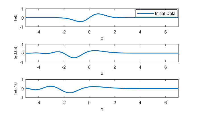
Figure 1: Solution of the Cauchy problem for (4.1) with the initial data (9.5).

The potential (9.5) has one eigenvalue which was computed numerically, $\lambda_{1}\approx-0.0138384593995$ with the corresponding norming constants $\alpha_{1}^{-}\approx 0.2055954681199$ and $\alpha_{1}^{+}\approx 0.0416040800785$. The reflection coefficients $s^{-}(\rho)$ and $s^{+}(\rho)$ where computed as explained in subsection 9.1 on the interval $\left(-500,500\right)$. This computation of the scattering data took less than a second in Matlab2017 on a Laptop computer equipped with an Intel Core i7 processor.

The inverse scattering problems were solved as explained in subsection 9.2 with five equations in the truncated systems (9.2) used for $x<0$ and (9.3) for $x>0$. The elapsed time to obtain Figure 1 was 9 sec.

Notice that after solving the direct scattering problem and the inverse scattering problem for $t=0$ the potential (9.5) on the interval $\left(-5,7\right)$ was recovered with the absolute error of $1.5\cdot 10^{-3}$.

Example 9.2.

Consider the Cauchy problem for the KdV equation (4.1) with the initial data in the form of the reflectionless potential

$$q(x)=-\frac{c}{2}\operatorname*{sech}{}^{2}\left(\frac{\sqrt{c}x}{2}\right).$$ (9.6)

The corresponding solution is the solitary wave

$$u(x,t)=-\frac{c}{2}\operatorname*{sech}{}^{2}\left(\frac{\sqrt{c}\left(x-ct\right)}{2}\right).$$

On Figure 2 the computed solution is presented for $c=\pi$ and $t=0,0.5,1$. Numerical solution of the direct scattering problem gave us the reflection coefficient equal to zero with the accuracy $2\cdot 10^{-4}$, and the only eigenvalue $\lambda_{1}\approx-0.78539816329$, while its exact value is $-c/4=-0.78539816339\ldots$ (the difference in the 10-th digit). The corresponding norming constants are $\alpha_{1}^{\pm}=\sqrt{\pi}$ which were computed with the accuracy $2.9\cdot 10^{-5}$. The solutions of the inverse scattering problems were obtained with five equations in the truncated systems (9.2) used for $x<0$ and (9.3) for $x>0$.

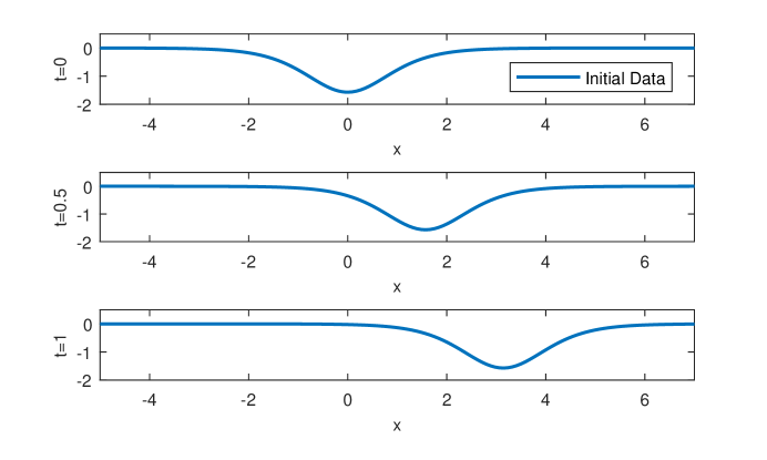
Figure 2: Solution of the Cauchy problem for (4.1) with the initial data (9.6).

After solving the direct scattering problem and the inverse scattering problem for $t=0$ the potential on the interval $\left(-5,7\right)$ was recovered with the absolute error of $8\cdot 10^{-4}$, and for subsequent times the error did not grow. For example, for $t=1$ the absolute error was $2.4\cdot 10^{-4}$.

Example 9.3.

Consider the Cauchy problem for the KdV equation (4.1) with the initial data

$$q(x)=\left\{\begin{array}[c]{cc}e^{x}\cos 4x,&x<0,\\ e^{-x}J_{0}(2x),&x>0,\end{array}\right.$$ (9.7)

where $J_{0}(z)$ stands for the Bessel function of the first kind of order zero. The graph of this potential is presented on Figure 3. Its first derivative is discontinuous.

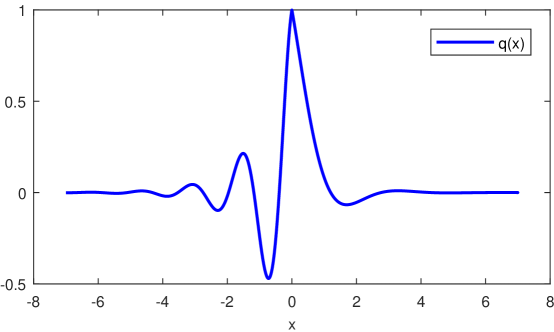
Figure 3: Graph of the potential (9.7).

On Figure the corresponding solution of the Cauchy problem for (4.1) is presented. It was obtained with nine equations in the truncated systems (with five equations it was only slightly less accurate). After solving the direct scattering problem and the inverse scattering problem for $t=0$ the potential (9.7) on the interval $\left(-7,7\right)$ was recovered with the absolute error of $6\cdot 10^{-3}$.

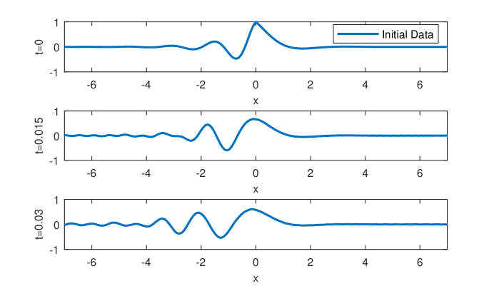
Figure 4: Solution of the Cauchy problem for (4.1) with the initial data (9.7).

Conclusions

A method for practical realization of the inverse scattering transform method for the Korteweg–de Vries equation is proposed. It is accurate, efficient and relatively simple for implementation. The applicability of the finite section method to the system of linear algebraic equations, which arises when solving the inverse scattering problem, is proved. Numerical examples are provided. Similar approach can be derived for other integrable non-linear equations, such as the nonlinear Schrödinger equation.

Appendix A Recurrent integration procedure for the coefficients of the representations

Here we recall the result from [15] concerning the coefficients $\left\{a_{n}\right\}$ and $\left\{d_{n}\right\}$ and obtain by analogy similar relations for the coefficients $\left\{b_{n}\right\}$ and $\left\{c_{n}\right\}$. Denote

$$\eta(x):=e(\frac{i}{2},x)\int_{0}^{x}\frac{dt}{e^{2}(\frac{i}{2},t)}$$ (A.1)

and

$$\xi(x):=g(\frac{i}{2},x)\int_{x}^{0}\frac{dt}{g^{2}(\frac{i}{2},t)}.$$ (A.2)

These solutions of (2.2) with $\lambda=-1/4$ satisfy the asymptotic relations $\eta(x)=e^{\frac{x}{2}}\left(1+o(1)\right)$, $x\rightarrow\infty$ and $\xi(x)=e^{-\frac{x}{2}}\left(1+o(1)\right)$, $x\rightarrow-\infty$, respectively. Computation of all coefficients can be performed acording to the following steps.

1. The coefficients $a_{0}$, $b_{0}$, $c_{0}$ and $d_{0}$ have the form

   $$a_{0}(x) =e(\frac{i}{2},x)e^{\frac{x}{2}}-1\quad\text{and}\quad b_{0}(x)=g(\frac{i}{2},x)e^{-\frac{x}{2}}-1,$$

   $$d_{0}(x) =a_{0}^{\prime}(x)-\frac{a_{0}(x)}{2}+\frac{1}{2}\int_{x}^{\infty}q(t)dt,$$ (A.3)

   $$c_{0}(x) =b_{0}^{\prime}(x)+\frac{b_{0}(x)}{2}-\frac{1}{2}\int_{-\infty}^{x}q(t)dt$$

2. The subsequent coefficients $a_{n}$ and $b_{n}$ together with their derivatives can be computed as follows

   $$a_{n}(x) =a_{0}(x)-2e^{\frac{x}{2}}\left(\eta(x)J_{1,n}(x)-e(\frac{i}{2},x)J_{2,n}(x)\right),$$

   $$b_{n}(x) =b_{0}(x)+2e^{-\frac{x}{2}}\left(\xi(x)I_{1,n}(x)-g(\frac{i}{2},x)I_{2,n}(x)\right),$$

   $$a_{n}^{\prime}(x) =a_{0}^{\prime}(x)-2\left(e^{\frac{x}{2}}\eta(x)\right)^{\prime}J_{1,n}(x)-2e^{\frac{x}{2}}\eta(x)J_{1,n}^{\prime}(x)$$

   $$+2\left(e^{\frac{x}{2}}e(\frac{i}{2},x)\right)^{\prime}J_{2,n}(x)+2e^{\frac{x}{2}}e(\frac{i}{2},x)J_{2,n}^{\prime}(x),$$ (A.4)

   $$b_{n}^{\prime}(x) =b_{0}^{\prime}(x)+2\left(e^{-\frac{x}{2}}\xi(x)\right)^{\prime}I_{1,n}(x)+2e^{-\frac{x}{2}}\xi(x)I_{1,n}^{\prime}(x)$$

   $$-2\left(e^{-\frac{x}{2}}g(\frac{i}{2},x)\right)^{\prime}I_{2,n}(x)-2e^{-\frac{x}{2}}g(\frac{i}{2},x)I_{2,n}^{\prime}(x),$$

   where

   $$J_{1,n}(x)=J_{1,n-1}(x)-e^{-\frac{x}{2}}e(\frac{i}{2},x)a_{n-1}(x)-\int_{x}^{\infty}\left(e(\frac{i}{2},t)e^{-\frac{t}{2}}\right)^{\prime}a_{n-1}(t)dt,$$ (A.5)

   $$J_{2,n}(x)=J_{2,n-1}(x)-e^{-\frac{x}{2}}\eta(x)a_{n-1}(x)-\int_{x}^{\infty}\left(\eta(t)e^{-\frac{t}{2}}\right)^{\prime}a_{n-1}(t)dt$$ (A.6)

   $$I_{1,n}(x)=I_{1,n-1}(x)+e^{\frac{x}{2}}g(\frac{i}{2},x)b_{n-1}(x)-\int_{-\infty}^{x}\left(g(\frac{i}{2},t)e^{\frac{t}{2}}\right)^{\prime}b_{n-1}(t)dt,$$ (A.7)

   and

   $$I_{2,n}(x)=I_{2,n-1}(x)+e^{\frac{x}{2}}\xi(x)b_{n-1}(x)-\int_{-\infty}^{x}\left(\xi(t)e^{\frac{t}{2}}\right)^{\prime}b_{n-1}(t)dt.$$ (A.8)

   ($J_{1,0}(x)=J_{2,0}(x)=I_{1,0}(x)=I_{2,0}(x)\equiv 0$), and for $J_{1,n}^{\prime}(x)$, $J_{2,n}^{\prime}(x)$, $I_{1,n}(x)$ and $I_{2,n}(x)$ the following relations are obtained from (A.5)-(A.8),

   $$J_{1,n}^{\prime}(x)=J_{1,n-1}^{\prime}(x)-e^{-\frac{x}{2}}e(\frac{i}{2},x)a_{n-1}^{\prime}(x),$$ (A.9)

   $$J_{2,n}^{\prime}(x)=J_{2,n-1}^{\prime}(x)-e^{-\frac{x}{2}}\eta(x)a_{n-1}^{\prime}(x),$$ (A.10)

   $$I_{1,n}^{\prime}(x)=I_{1,n-1}^{\prime}(x)+e^{\frac{x}{2}}g(\frac{i}{2},x)b_{n-1}^{\prime}(x)$$

   and

   $$I_{2,n}^{\prime}(x)=I_{2,n-1}^{\prime}(x)+e^{\frac{x}{2}}\xi(x)b_{n-1}^{\prime}(x).$$

3. The coefficients $d_{n}$ and $c_{n}$ can be computed with the aid of the relations

   $$d_{n+1}(x)=d_{n}(x)+a_{n+1}^{\prime}(x)-a_{n}^{\prime}(x)-\frac{1}{2}\left(a_{n+1}(x)+a_{n}(x)\right),\quad n=0,1,\ldots$$ (A.11)

   and

   $$c_{n+1}(x)=c_{n}(x)+b_{n+1}^{\prime}(x)-b_{n}^{\prime}(x)+\frac{1}{2}\left(b_{n+1}(x)+b_{n}(x)\right),\quad n=0,1,\ldots.$$

References

- [1] M. J. Ablowitz, Nonlinear dispersive waves: asymptotic analysis and solitons. Cambridge University Press, Cambridge, 2011.
- [2] M. J. Ablowitz, P. Clarkson, Solitons, nonlinear evolution equations and inverse scattering. Cambridge University Press, Cambridge, 1991.
- [3] M. J. Ablowitz, H. Segur, Solitons and the inverse scattering transform. Society for Industrial and Applied Mathematics (SIAM), Philadelphia, 2000.
- [4] M. Abramovitz, I. A. Stegun, Handbook of mathematical functions. Dover, New York, 1972.
- [5] E. N. Aksan, A. Özdes, Numerical solution of Korteweg–de Vries equation by Galerkin B-spline finite element method. Applied Mathematics and Computation 175 (2006) 1256–1265.
- [6] G. A. Baker, V. A. Dougalis, O. A. Karakashian, Convergence of Galerkin approximations for the Korteweg–de Vries equation. Mathematics of Computation 40 (1983) 419-433.
- [7] A. Böttcher, B. Silbermann, Introduction to large truncated Toeplitz matrices. Springer, New York, 1999.
- [8] A. Böttcher, B. Silbermann, Analysis of Toeplitz operators. Springer, Berlin/Heidelberg/New York, 2006.
- [9] Kh. Chadan, D. Colton, L. Päivärinta and W. Rundell, An introduction to inverse scattering and inverse spectral problems. SIAM, Philadelphia, 1997.
- [10] Kh. Chadan, P. C. Sabatier, Inverse problems in quantum scattering theory. Springer, New York, 1989.
- [11] J. B. Conway, A Course in Functional Analysis. Springer, New York, 1990.
- [12] C. Courtès, F. Lagoutière, F. Rousset, Error estimates of finite difference schemes for the Korteweg–de Vries equation. IMA Journal of Numerical Analysis 40 (2020) 628–685.
- [13] M. Dehghan, A. Shokri, A numerical method for KdV equation using collocation and radial basis functions. Nonlinear Dynamics 50 (2007) 111–120.
- [14] B. B. Delgado, K. V. Khmelnytskaya, V. V. Kravchenko, A representation for Jost solutions and an efficient method for solving the spectral problem on the half line. Mathematical Methods in the Applied Sciences 42 (2019) 7359–7366.
- [15] B. B. Delgado, K. V. Khmelnytskaya, V. V. Kravchenko, A representation for Jost solutions and an efficient method for solving the spectral problem on the half line. Mathematical Methods in the Applied Sciences 43 (2020) 9304–9319.
- [16] C. S. Gardner, J. M. Greene, M. D. Kruskal, R. M. Miura, Method for solving the Korteweg–de Vries equation. Phys. Rev. Lett. 19, issue 19 (1967) 1095–1097.
- [17] I. Gradshteyn, I. Ryzhik, Table of integrals, series, and products. Academic Press, 1980.
- [18] S. M. Grudsky, A. Rybkin, Soliton theory and Hankel operators. SIAM Journal on Mathematical Analysis 47, issue 3 (2015) 2283-2323.
- [19] S. M. Grudsky, A. Rybkin, On the trace-class property of Hankel operators arising in the theory of the Korteweg–de Vries equation. Mathematical Notes, 104, issue 3 (2018) 377-394.
- [20] S. M. Grudsky, A. Rybkin, On classical solutions of the KdV equation. Proceedings of London Mathematical Society 121, issue 2 (2020) 354-371.
- [21] V. V. Kravchenko, Applied pseudoanalytic function theory. Frontiers in Mathematics, Birkhäuser, Basel, 2009.
- [22] V. V. Kravchenko, On a method for solving the inverse scattering problem on the line. Mathematical Methods in the Applied Sciences 42 (2019), 1321-1327.
- [23] V. V. Kravchenko, Direct and inverse Sturm-Liouville problems: A method of solution, Birkhäuser, Cham, 2020.
- [24] V. V. Kravchenko, R. M. Porter, Spectral parameter power series for Sturm-Liouville problems. Mathematical Methods in the Applied Sciences 33 (2010), 459–468.
- [25] V. V. Kravchenko, E. L. Shishkina, S. M. Torba, A transmutation operator method for solving the inverse quantum scattering problem. Inverse Problems 36 (2020), 125007 (23pp).
- [26] V. V. Kravchenko, S. M. Torba, A direct method for solving inverse Sturm-Liouville problems. Inverse Problems 37 (2021), 015015 (32pp).
- [27] G. L. Lamb Elements of soliton theory. John Wiley & Sons, New York-Chichester-Brisbane-Toronto, 1980.
- [28] B. M. Levitan, Inverse Sturm-Liouville problems, VSP, Zeist, 1987.
- [29] V. A. Marchenko, Sturm-Liouville operators and applications: revised edition, AMS Chelsea Publishing, 2011.
- [30] S. G. Mihlin, The numerical performance of variational methods, Wolters-Noordhoff publishing, Groningen, The Netherlands, 1971.
- [31] A. P. Prudnikov, Y. A. Brychkov, O. I. Marichev, Integrals and series. Vol. 2. Special functions, Gordon & Breach Science Publishers, New York, 1986.
- [32] A. Rashid, Numerical solution of Korteweg–de Vries equation by the Fourier pseudospectral method. Bull. Belg. Math. Soc. Simon Stevin 14 (2007) 709–721.
- [33] W. Rudin Real and Complex Analysis. McGraw-Hill, 1986.
- [34] J. K. Shaw, Mathematical principles of optical fiber communications. SIAM, Philadelphia, 2004.
- [35] E. L. Shishkina and S. M. Sitnik, Transmutations, singular and fractional differential equations with applications to mathematical physics. Elsevier, Amsterdam, 2020.
- [36] V. A. Yurko, Introduction to the theory of inverse spectral problems. Fizmatlit, Moscow, 2007 (in Russian).
- [37] V. E. Zakharov, A. B. Shabat, Exact theory of two-dimensional self-focusing and one-dimensional self-modulation of waves in nonlinear media. Soviet Physics-JETP 34 (1972) 62–69.