Sample-Efficient Reinforcement Learning of Partially Observable Markov Games

Abstract

This paper considers the challenging tasks of Multi-Agent Reinforcement Learning (MARL) under partial observability, where each agent only sees her own individual observations and actions that reveal incomplete information about the underlying state of system. This paper studies these tasks under the general model of multiplayer general-sum Partially Observable Markov Games (POMGs), which is significantly larger than the standard model of Imperfect Information Extensive-Form Games (IIEFGs). We identify a rich subclass of POMGs—weakly revealing POMGs—in which sample-efficient learning is tractable. In the self-play setting, we prove that a simple algorithm combining optimism and Maximum Likelihood Estimation (MLE) is sufficient to find approximate Nash equilibria, correlated equilibria, as well as coarse correlated equilibria of weakly revealing POMGs, in a polynomial number of samples when the number of agents is small. In the setting of playing against adversarial opponents, we show that a variant of our optimistic MLE algorithm is capable of achieving sublinear regret when being compared against the optimal maximin policies. To our best knowledge, this work provides the first line of sample-efficient results for learning POMGs.

1 Introduction

This paper studies Multi-Agent Reinforcement Learning (MARL) under partial observability, where each player tries to maximize her own utility via interacting with an unknown environment as well as other players. In addition, each agent only sees her own observations and actions, which reveal incomplete information about the underlying state of system. A large number of real-world applications can be cast into this framework: in Poker, cards in a player’s hand are hidden from the other players; in many real-time strategy games, players have only access to their local observations; in multi-agent robotic systems, agents with first-person cameras have to cope with noisy sensors and occlusions. While practical MARL systems have achieved remarkable success in a set of partially observable problems including Poker (Brown and Sandholm, 2019), Starcraft (Vinyals et al., 2019), Dota (Berner et al., 2019) and autonomous driving (Shalev-Shwartz et al., 2016), the theoretical understanding of MARL under partial observability remains very limited.

The combination of partial observability with multiagency introduces a number of unique challenges. The non-Markovian nature of the observations forces the agent to maintain memory and reason about beliefs of the system state, all while exploring to collect information about the environment. Consequently, well-known complexity-theoretic results show that learning and planning in partially observable environments is statistically and computationally intractable even in the single-agent setting (Papadimitriou and Tsitsiklis, 1987; Mundhenk et al., 2000; Vlassis et al., 2012; Mossel and Roch, 2005). The presence of interaction between multiple agents further complicates the partially observable problems. In addition to dealing with the adaptive nature of other players who can adjust their strategies according to the learner’s past behaviors, the learner is further required to discover and exploit the information asymmetry due to the separate observations of each agent.

As a result, prior theoretical works on partially observable MARL have been mostly focused on a small subset of problems with strong structural assumptions. For instance, the line of works on Imperfect Information Extensive-Form Games (IIEFG) (see, e.g., Zinkevich et al., 2007; Gordon, 2007; Farina and Sandholm, 2021; Kozuno et al., 2021) assumes tree-structured transition with small depth as well as a special type of emission which can be represented as information sets. In contrast, this paper considers a more general mathematical model known as Partially Observable Markov Games (POMGs). POMGs are the natural extensions of both Partially Observable Markov Decision Processes (POMDPs)—the standard model for single-agent partially observable RL, and Markov Games (Shapley, 1953)—the standard model for fully observable MARL. Despite the complexity barriers of learning partially observable systems apply to POMGs, they are of a worst-case nature, which do not preclude efficient algorithms for learning interesting subclasses of POMGs. This motivates us to ask the following question:

Can we develop efficient algorithms that learn a rich class of POMGs?

In this paper, we provide the first positive answer to the highlighted question in terms of the sample efficiency. We identify a rich family of tractable POMGs—weakly revealing POMGs (see Section 3). The weakly revealing condition only requires the joint observations of all agents to reveal certain amount of information about the latent states, which is satisfied in many real-world applications. The condition rules out the pathological instances where no player has any information to distinguish latent states, which prevents efficient learning in the worst case.

In the self-play setting where the algorithm can control all the players to learn the equilibria by playing against itself, this paper proposes a new simple algorithm—Optimistic Maximum Likelihood Estimation for Learning Equilibria (OMLE-Equilibrium). As the name suggests, it combines optimism, MLE principles with equilibria finding subroutines. The algorithm provably finds approximate Nash equilibria, coarse correlated equilibria and correlate equilibria of any weakly-revealing POMGs using a number of samples polynomial in all relevant parameters.

In the setting of playing against adversarial opponents, we measure the performance of our algorithm by comparing against the optimal maximin policies. We first prove that learning in this setting is hard if each player can only see her own observations and actions. Nevertheless, if the agent is allowed to access other players’ observations and actions after each episode of play (e.g., watch the replays of the games from other players’ perspectives afterwards), then we can design a new algorithm OMLE-Adversary which achieves sublinear regret.

To our best knowledge, this is the first line of provably sample-efficient results for learning rich classes of POMGs. Importantly, the classes of problems that can be learned in this paper are significantly larger than known tractable classes of MARL problems under partial observability.

1.1 Technical novelty

This paper builds upon the recent progress in learning single-agent POMDPs (Liu et al., 2022a), which identifies the class of weakly revealing POMDPs and develops OMLE algorithm for learning the optimal policy. Besides obtaining a completely new set of results in the multi-agent setting, we here highlight a few contributions and technical novelties of this paper comparing to Liu et al. (2022a).

• This paper rigorously formulates the models, related concepts and learning objectives of multi-player general-sum POMGs, and provides the first line of sample-efficient learning results.

• Extending the weakly revealing conditions into the multi-agent setting lead to two natural candidates: either (a) joint observations or (b) individual observations are required to weakly reveal the state information. This paper shows the former (the weaker assumption) suffices to guarantee tractability.

• Results in the self-play setting requires careful design of optimistic planning algorithms that effectively address the game-theoretical aspects of the problem under partial observability. We achieve this by Subroutine 1, which is even distinct from the standard techniques for learning MGs.

• The discussions and results in the setting of playing against adversarial opponents are completely new, and unique to the multi-agent setup.

1.2 Related Works

Reinforcement learning has been extensively studied in the single-agent fully-observable setting (see, e.g., Azar et al., 2017; Dann et al., 2017; Jin et al., 2018, 2020a; Zanette et al., 2020; Jiang et al., 2017; Jin et al., 2021a, and the references therein) . For the purpose of this paper, we focus on reviewing existing works on partially observable RL and multi-agent RL in the exploration setting.

Markov games

In recent years, there has been growing interest in studying Markov games (Shapley, 1953) — the standard generalization of MDPs from the single-player setting to the multi-player setting. Various sample-efficient algorithms have been designed for either two-player zero-sum MGs (e.g., Brafman and Tennenholtz, 2002; Wei et al., 2017; Bai and Jin, 2020; Liu et al., 2021; Bai et al., 2020; Xie et al., 2020; Jin et al., 2021b) or multi-player general-sum MGs (e.g., Liu et al., 2021; Jin et al., 2021c; Song et al., 2021; Daskalakis et al., 2022). However, all these works rely on the states being fully observable, while the POMGs studied in this paper allow states to be only partially observable, which strictly generalizes MGs.

POMDPs

POMDPs generalize MDPs from the fully observable setting to the partially observable setting. It is well-known that in POMDPs both planning (Papadimitriou and Tsitsiklis, 1987; Vlassis et al., 2012) and model estimation (Mossel and Roch, 2005) are computationally hard in the worst case. Besides, reinforcement learning of POMDPs is also known to be statistically hard: Krishnamurthy et al. (2016) proved that finding a near-optimal policy of a POMDP in the worst case requires a number of samples that is exponential in the episode length. The hard instances are those pathological POMDPs where the observations contain no useful information for identifying the system dynamics. Nonetheless, these hardness results are all in the worst-case sense and there are still many intriguing positive results on sample-efficient learning of subclasses of POMDPs. For example, Guo et al. (2016); Azizzadenesheli et al. (2016); Jin et al. (2020b) applied spectral methods to learning undercomplete POMDPs and Liu et al. (2022a) developed the optimistic MLE approach for learning both undercomplete and overcomplete POMDPs. We refer interested readers to Liu et al. (2022a) for a thorough review of existing results on POMDPs.

In terms of algorithmic design, our algorithms build upon the optimistic MLE methodology developed in Liu et al. (2022a). Compared to Liu et al. (2022a), our main algorithmic contribution lies in the design of the optimistic equilibrium computation subroutine in the self-play setting and the optimistic maximin policy design in the adversarial setting. In terms of analysis, our proofs requrie new techniques tailored to controlling game-theoretic regret, in addition to the OMLE guarantees imported from Liu et al. (2022a). For more detailed explanations of our technical contribution, please refer to Section 1.1.

Imperfect-information extensive-form games

In the literature on game theory, there is a long history of learning Imperfect-Information Extensive-Form Games with perfect recall (IIEFGs), (see, e.g., Zinkevich et al., 2007; Gordon, 2007; Farina et al., 2020; Farina and Sandholm, 2021; Kozuno et al., 2021) and the references therein. IIEFGs can be viewed as special cases of POMGs with tree-structured transition and deterministic emission (which are also known as information sets). As a result, IIEFGs can not efficiently represent POMGs with general transition and stochastic emission (see Appendix A), and thus sample-efficient learning results for IIEFGs does not imply sample-efficient learning of POMGs. On the other hand, we show that all IIEFGs can be efficiently represented by $1$-weakly revealing POMGs (see Appendix A). Therefore, all algorithms and theoretical results developed in this paper can immediately used to learn IIEFGs with a polynomial sample complexity.

Decentralized POMDPs

There is another classic model for studying multi-agent partially observable RL, named decentralized POMDPs (e.g., Oliehoek, 2012; Oliehoek and Amato, 2016), which is a special subclass of POMGs where all players share a common reward target. Compared to general POMGs, decentralized POMDPs can only simulate cooperative relations among players, while general POMGs can model both cooperative and competitive relations. Besides, most works (e.g., Nair et al., 2003; Bernstein et al., 2005; Oliehoek et al., 2008; Szer et al., 2012; Dibangoye et al., ; Liu et al., 2017; Amato et al., 2019) along this direction mainly focus on the computational complexity of planning with known models or simulators instead of the sample efficiency of learning from interactions (as in this paper), which requires learning and estimating the unknown environment while balancing the tradeoff between exploration and exploitation.

Interactive POMDPs

Another related model is Interactive POMDPs (I-POMDPs) (Gmytrasiewicz and Doshi, 2005; Doshi et al., 2009), which generalizes POMDPs to handle the presence of other agents by augmenting the latent state with behavior models of other agents. Since I-POMDPs are strictly more general than POMDPs, they are also less understood in theory than POMDPs. Noticably, I-POMDPs can only efficiently handle the problems where the number of possible models of other agents is not too large. For the POMGs model considered in this paper, even in the simplest setting of two-player zero-sum games, an agent can choose from doubly exponentially many different history-dependent strategies. As a result, I-POMDPs cannot efficiently simulate POMGs without using a latent state space that is doubly exponentially large.

2 Preliminary

In this paper, we consider Partially Observable Markov Games (POMGs) in its most generic—multiplayer general-sum form. Formally, we denote a tabular episodic POMG with $n$ players by tuple $(H,\mathcal{S},\{\mathcal{A}_{i}\}_{i=1}^{n},$
$\{\mathcal{O}_{i}\}_{i=1}^{n};\mathbb{T},\mathbb{O},\mu_{1};\{r_{i}\}_{i=1}^{n})$, where $H$ denotes the length of each episode, $\mathcal{S}$ the state space with $|\mathcal{S}|=S$, $\mathcal{A}_{i}$ denotes the action space for the $i^{\rm th}$ player with $|\mathcal{A}_{i}|=A_{i}$. We denote by $\bm{a}:=(a_{1},\cdots,a_{n})$ the joint actions of all $n$ players, and by $\mathcal{A}:=\mathcal{A}_{1}\times\ldots\times\mathcal{A}_{n}$ the joint action space with $|\mathcal{A}|=A=\prod_{i}A_{i}$. $\mathbb{P}=\{\mathbb{P}_{h}\}_{h\in[H]}$ is the collection of transition matrices, so that $\mathbb{P}_{h}(\cdot|s,\bm{a})\in\Delta_{\mathcal{S}}$ gives the distribution of the next state if joint actions $\bm{a}$ are taken at state $s$ at step $h$. $\mu_{1}$ denotes the distribution of the initial state $s_{1}$. $\mathcal{O}_{i}$ denotes the observation space for the $i^{\rm th}$ player with $|\mathcal{O}_{i}|=O_{i}$. We denote by $\mathbf{o}:=(o_{1},\ldots,o_{n})$ the joint observations of all $n$ players, and by $\mathcal{O}:=\mathcal{O}_{1}\times\ldots\times\mathcal{O}_{n}$ with $|\mathcal{O}|=O=\prod_{i}O_{i}$. $\mathbb{O}=\{\mathbb{O}_{h}\}_{h\in[H]}\subseteq\mathbb{R}^{O\times S}$ is the collection of joint emission matrices, so that $\mathbb{O}_{h}(\cdot|s)\in\Delta_{\mathcal{O}}$ gives the emission distribution over the joint observation space $\mathcal{O}$ at state $s$ and step $h$. Finally $r_{i}=\{r_{i,h}\}_{h\in[H]}$ is the collection of known reward functions for the $i^{\text{th}}$ player, so that $r_{i,h}(o_{i})\in[0,1]$ gives the deterministic reward received by the $i^{\text{th}}$ player if she observes $o_{i}$ at step $h$. We remark that since the relation among the rewards of different players can be arbitrary, this model of POMGs subsumes both the cooperative and the competitive settings in partially observable MARL.

In a POMG, the states are always hidden from all players, and each player only observes her own individual observations and actions. That is, each player can not see the observations and actions of the other players. At the beginning of each episode, the environment samlpes $s_{1}$ from $\mu_{1}$. At each step $h\in[H]$, each player $i$ observes her own observation $o_{i,h}$ where $\mathbf{o}_{h}:=(o_{1,h},\ldots,o_{n,h})$ are jointly sampled from $\mathbb{O}_{h}(\cdot\mid{s_{h}})$. Then each player $i$ receives reward $r_{i,h}(o_{i,h})$ and picks action $a_{i,h}\in\mathcal{A}_{i}$ simultaneously. After that the environment transitions to the next state $s_{h+1}\sim\mathbb{P}_{h}(\cdot|s_{h},\bm{a}_{h})$ where $\mathbf{a}_{h}:=(a_{1,h},\ldots,a_{n,h})$. The current episode terminates immediately once $s_{H+1}$ is reached.

Policy, value function

To define different types of polices, we extend the conventions in fully observable Markov games (Jin et al., 2021c) to the partially observable settings. A (random) policy $\pi_{i}$ of the $i^{\rm th}$ player is a map $\pi_{i}:\Omega\times\bigcup_{h=1}^{H}\left((\mathcal{O}_{i}\times\mathcal{A}_{i})^{h-1}\times\mathcal{O}_{i}\right)\rightarrow\mathcal{A}_{i}$, which maps a random seed $\omega$ from space $\Omega$ and a history of length $h\in[H]$—say $\tau_{i,h}:=(o_{i,1},a_{i,1},\cdots,o_{i,h})$, to an action in $\mathcal{A}_{i}$. To execute policy $\pi_{i}$, we first draw a random sample $\omega$ at the beginning of the episode. Then, at each step $h$, the $i^{\rm th}$ player simply takes action $\pi_{i}(\omega,\tau_{i,h})$. We note here $\omega$ is shared among all steps $h\in[H]$. $\omega$ encodes both the correlation among steps and the individual randomness of each step. We further say a policy $\pi_{i}$ is deterministic if $\pi_{i}(\omega,\tau_{i,h})=\pi_{i}(\tau_{i,h})$ which is independent of the choice of $\omega$.

By definition, a random policy is equivalent to a mixture of deterministic policies because given a fixed $\omega$ the decision of $\pi_{i}$ on any history is deterministic. With slight abuse of notation, we use $\pi_{i}(\omega,\cdot)$ to refer to the deterministic policy realized by policy $\pi_{i}$ and a fixed $\omega$. We denote the set of all policies of the $i^{\rm th}$ player by $\Pi_{i}$ and the set of all deterministic ones by $\Pi_{i}^{\rm det}$.

A joint (potentially correlated) policy is a set of policies $\{\pi_{i}\}_{i=1}^{n}$, where the same random seed $\omega$ is shared among all agents, which we denote as $\pi=\pi_{1}\odot\pi_{2}\odot\ldots\odot\pi_{n}$. We also denote $\pi_{-i}=\pi_{1}\odot\ldots\pi_{i-1}\odot\pi_{i+1}\odot\ldots\odot\pi_{n}$ to be the joint policy excluding the $i^{\rm th}$ player. A special case of joint policy is the product policy where the random seed has special form $\omega=(\omega_{1},\ldots,\omega_{n})$, and for any $i\in[n]$, $\pi_{i}$ only uses the randomness in $\omega_{i}$, which is independent of remaining $\{\omega_{j}\}_{j\neq i}$, which we denote as $\pi=\pi_{1}\times\pi_{2}\times\ldots\times\pi_{n}$.

We define the value function $V^{\pi}_{i}$ as the expected cumulative reward that the $i^{\text{th}}$ player will receive if all players follow joint policy $\pi$:

$$\textstyle V^{\pi}_{i}\mathrel{\mathop{:}}=\mathbb{E}_{\pi}\left[\sum_{h=1}^{H}r_{i,h}(o_{i,h})\right].$$ (1)

where the expectation is taken over the randomness in the initial state, the transitions, the emissions, and the random seed $\omega$ in policy $\pi$.

Best response and strategy modification

For any strategy $\pi_{-i}$, the best response of the $i^{\rm th}$ player is defined as a policy of the $i^{\text{th}}$ player, which is independent of the randomness in $\pi_{-i}$ and achieves the highest value for herself conditioned on all other players deploying $\pi_{-i}$. Formally, the best response is the maximizer of $\max_{\pi^{\prime}_{i}}V_{i}^{\pi^{\prime}_{i}\times\pi_{-i}}$ whose value we also denote as $V_{i}^{\dagger,\pi_{-i}}$ for simplicity. By its definition, we know the best response can always be achieved by deterministic policies.

A strategy modification for the $i^{\rm th}$ player is a map $\phi_{i}:\Pi_{i}^{\rm det}\rightarrow\Pi_{i}^{\rm det}$, which maps a deterministic policy in $\Pi_{i}^{\rm det}$ to another one in it. For any such strategy modification $\phi_{i}$, we can naturally extend its domain and image to include random policies, i.e., define its extension $\phi_{i}:\Pi_{i}\rightarrow\Pi_{i}$ as follows: by definition, a random policy $\pi$ can be expressed as a mixture of deterministic policies, i.e., as $\pi(\omega,\cdot)$ (a deterministic policy for a fixed $\omega$) with a distribution over $\omega$. Then if we apply map $\phi_{i}$ on random policy $\pi$, we can define the resulting random policy (denoted as $\phi_{i}\diamond\pi_{i}$) as $\phi_{i}(\pi_{i}(\omega,\cdot))$ (again a deterministic policy for a fixed $\omega$) with the same distribution over $\omega$. For any joint policy $\pi$, we define the best strategy modification of the $i^{\text{th}}$ player as the maximizer of $\max_{\phi_{i}}V_{i}^{(\phi_{i}\diamond\pi_{i})\odot\pi_{-i}}$.

Different from the best response, which is completely independent of the randomness in $\pi_{-i}$, the best strategy modification changes the policy of the $i^{\rm th}$ player while still utilizing the shared randomness among $\pi_{i}$ and $\pi_{-i}$. Therefore, the best strategy modification is more powerful than the best response: formally one can show that $\max_{\phi_{i}}V_{i}^{(\phi_{i}\diamond\pi_{i})\odot\pi_{-i}}\geq\max_{\pi^{\prime}_{i}}V_{i}^{\pi^{\prime}_{i}\times\pi_{-i}}$ for any policy $\pi$.

2.1 Learning objectives

We focus on three classic equilibrium concepts in game theory—Nash Equilibrium, Correlated Equilibrium (CE) and Coarse Correlated Equilibrium (CCE). First, a Nash equilibrium is defined as a product policy in which no player can increase her value by changing only her own policy. Formally,

Definition 1 (Nash Equilibrium).

A product policy $\pi$ is a Nash equilibrium if $V_{i}^{{\dagger},\pi_{-i}}=V_{i}^{\pi}$ for all $i\in[n]$. A product policy $\pi$ is an $\epsilon$-approximate Nash equilibrium if $V_{i}^{\dagger,\pi_{-i}}\leq V_{i}^{\pi}+\epsilon$ for all $i\in[n]$.

The Nash-regret of a sequence of product policies is the cumulative violation of the Nash condition.

Definition 2 (Nash-regret).

Let $\pi^{k}$ denote the (product) policy deployed by an algorithm in the $k^{\text{th}}$ episode. After a total of $K$ episodes, the Nash-regret is defined as

$$\textstyle{\rm Regret}_{\rm Nash}(K)=\sum_{k=1}^{K}\max_{i\in[n]}{(V_{i}^{{\dagger},\pi_{-i}^{k}}-V_{i}^{\pi^{k}})}.$$

Second, a coarse correlated equilibrium is defined as a joint (potentially correlated) policy where no player can increase her value by unilaterally changing her own policy. Formally,

Definition 3 (Coarse Correlated Equilibrium).

A joint policy $\pi$ is a CCE if $V_{i}^{{\dagger},\pi_{-i}}\leq V_{i}^{\pi}$ for all $i\in[n]$. A joint policy $\pi$ is an $\epsilon$-approximate CCE if $V_{i}^{\dagger,\pi_{-i}}\leq V_{i}^{\pi}+\epsilon$ for all $i\in[n]$.

The only difference between Definition 1 and Definition 3 is that a Nash equilibrium has to be a product policy while a CCE can be correlated. Therefore, CCE is a relaxed notion of Nash equilibrium, and a Nash equilibrium is always a CCE. Similarly, we can define the CCE-regret for a sequence of potentially correlated policies as the cumulative vilolation of the CCE condition.

Definition 4 (CCE-regret).

Let $\pi^{k}$ denote the policy deployed by an algorithm in the $k^{\text{th}}$ episode. After a total of $K$ episodes, the CCE-regret is defined as

$$\textstyle{\rm Regret}_{\rm CCE}(K)=\sum_{k=1}^{K}\max_{i\in[n]}{(V_{i}^{{\dagger},\pi_{-i}^{k}}-V_{i}^{\pi^{k}})}.$$

Finally, a correlated equilibrium is defined as a joint (potentially correlated) policy where no player can increase her value by unilaterally applying any strategy modification. Formally,

Definition 5 (Correlated Equilibrium).

A joint policy $\pi$ is a CE if $\max_{\phi_{i}}V_{i}^{(\phi_{i}\diamond\pi_{i})\odot\pi_{-i}}=V_{i}^{\pi}$ for all $i\in[n]$. A joint policy $\pi$ is an $\epsilon$-approximate CE if $\max_{\phi_{i}}V_{i}^{(\phi_{i}\diamond\pi_{i})\odot\pi_{-i}}\leq V_{i}^{\pi}+\epsilon$ for all $i\in[m]$.

In Partially Observable Markov games, we always have that a Nash equilibrium is a CE, and a CE is a CCE. Finally, we define the CE-regret to be the cumulative violation of the CE condition.

Definition 6 (CE-regret).

Let $\pi^{k}$ denote the policy deployed by an algorithm in the $k^{\text{th}}$ episode. After a total of $K$ episodes, the CE-regret is defined as

$$\textstyle{\rm Regret}_{\rm CE}(K)=\sum_{k=1}^{K}\max_{i\in[n]}\max_{\phi_{i}}{(V_{i}^{(\phi_{i}\diamond\pi_{i}^{k})\odot\pi_{-i}^{k}}-V_{i}^{\pi^{k}})}.$$

3 Weakly Revealing Partially Observable Markov Games

In this section, we define the class of weakly revealing POMGs. To begin with, we consider undercomplete POMGs where there are more observations than hidden states, i.e., $O\geq S$. Formally, the family of $\alpha$-weakly revealing POMGs includes all POMGs, in which the $S^{\text{th}}$ singular value of each emission matrix $\mathbb{O}_{h}$ is lower bounded by $\alpha>0$.

Assumption 1 ($\alpha$-weakly revealing condition).

There exists $\alpha>0$, such that $\min_{h}\sigma_{S}(\mathbb{O}_{h})\geq\alpha$.

Assumption 1 is simply a robust version of the condition that the rank of each emission matrix is $S$, which guarantees that no two different latent state mixtures can generate the same observation distribution, i.e., $\mathbb{O}_{h}\nu_{1}\neq\mathbb{O}_{h}\nu_{2}$ for any different $\nu_{1},\nu_{2}\in\Delta_{\mathcal{S}}$. Intuitively, this guarantees that the joint observations of all agents contain sufficient information to distinguish any two different state mixtures. We remark that this is much weaker than requiring the individual observations of each agent contain sufficient information about the latent states. The weakly revealing condition is important in excluding those pathological POMGs where the observations contain no useful information for identifying the key parts of model dynamics.

Note that Assumption 1 never holds in the overcomplete setting ($S>O$) as it is impossible to distinguish any two latent state mixtures by only inspecting the observation distribution in a single step. To address this issue, we can instead inspect the observations for $m$-consecutive steps. To proceed, we define the $m$-step emission-action matrices

$$\{\mathbb{M}_{h}\in\mathbb{R}^{(A^{m-1}O^{m})\times S}\}_{h\in[H-m+1]}$$

as follows: Given an observation sequence $\bar{\mathbf{o}}$ of length $m$, initial state $s$ and action sequence $\bar{\mathbf{a}}$ of length $m-1$, we let $[\mathbb{M}_{h}]_{(\bar{\mathbf{a}},\bar{\mathbf{o}}),s}$ be the probability of receiving $\bar{\mathbf{o}}$ provided that the action sequence $\bar{\mathbf{a}}$ is used from state $s$ and step $h$:

$$\textstyle[\mathbb{M}_{h}]_{(\bar{\mathbf{a}},\bar{\mathbf{o}}),s}=\mathbb{P}(o_{h:h+m-1}=\bar{\mathbf{o}}\mid s_{h}=s,a_{h:h+m-2}=\bar{\mathbf{a}}),\quad\forall(\bar{\mathbf{a}},\bar{\mathbf{o}},s)\in\mathcal{A}^{m-1}\times\mathcal{O}^{m}\times\mathcal{S}.$$ (2)

Similar to the undercomplete setting, the weakly-revealing condition in the over-complete setting simply assumes the $S^{\text{th}}$ singular value of each $m$-step emission-action matrix is lower bounded.

Assumption 2 (multistep $\alpha$-weakly revealing condition).

There exists $m\in\mathbb{N}$, $\alpha>0$ such that $\min_{h}\sigma_{S}(\mathbb{M}_{h})\geq\alpha$ where $\mathbb{M}_{h}$ is the $m$-step emission matrix defined in (2).

Assumption 2 ensures that $m$-step consecutive observations shall contain sufficient information to distinguish any two different latent state mixtures. Note that Assumption 1 is a special case of Assumption 2 with $m=1$. Finally, we remark that the single-agent versions of Assumption 1 and 2 were first identified in Jin et al. (2020b) and Liu et al. (2022a) as sufficient conditions for sample-efficient learning of single-step and multi-step weakly revealing POMDPs (the single-agent version of POMGs), respectively.

4 Learning Equilibria with Self-play

In this section, we study the self-play setting where the algorithm can control all the players to learn the equilibria by playing against itself. We propose a new algorithm — Optimistic Maximum Likelihood Estimation for Learning Equilibria (OMLE-Equilibrium) that can provably find Nash equilibria, coarse correlated equilibria and correlate equilibria in any weakly-revealing partially observable Markov games using a number of samples polynomial in all relevant parameters.

4.1 Undercomplete partially observable Markov games

Algorithm 1 OMLE-Equilibrium

1:  Initialize: $\mathcal{B}^{1}=\{\hat{\theta}\in\Theta:~{}\min_{h}\sigma_{S}(\hat{\mathbb{O}}_{h})\geq\alpha\}$, $\mathcal{D}=\{\}$

2:  for $k=1,\ldots,K$ do

3:     compute $\pi^{k}=$Optimistic_Equilibrium$(\mathcal{B}^{k})$

4:     follow $\pi^{k}$ to collect a trajectory $\tau^{k}=(\mathbf{o}_{1}^{k},\mathbf{a}_{1}^{k},\ldots,\mathbf{o}_{H}^{k},\mathbf{a}_{H}^{k})$

5:     add $(\pi^{k},\tau^{k})$ into $\mathcal{D}$ and update

$$\mathcal{B}^{k+1}=\bigg{\{}\hat{\theta}\in\Theta:\sum_{(\pi,\tau)\in\mathcal{D}}\log\mathbb{P}_{{\hat{\theta}}}^{\pi}(\tau)\geq\max_{\theta^{\prime}\in\Theta}\sum_{(\pi,\tau)\in\mathcal{D}}\log\mathbb{P}^{\pi}_{{\theta^{\prime}}}(\tau)-\beta\bigg{\}}\bigcap\mathcal{B}^{1}$$

6:  output $\pi^{\rm out}$ that is sampled uniformly at random from $\{\pi^{k}\}_{k\in[K]}$

Subroutine 1 Optimistic_Equilibrium$(\mathcal{B})$

1:  for $i\in[n]$ do

2:     let $\overline{V}_{i}\in\mathbb{R}^{|\Pi^{\text{det}}_{1}|\times\cdots\times|\Pi^{\text{det}}_{n}|}$ with its $\pi^{\rm th}$ entry equal to $\sup_{\hat{\theta}\in\mathcal{B}}V_{i}^{\pi}(\hat{\theta})$ for $\pi\in\Pi_{1}\times\cdots\times\Pi_{n}$

3:  return $\textsc{Equilibrium}(\overline{V}_{1},\ldots,\overline{V}_{n})$

We first present the algorithm and results for learning undercomplete POMGs under Assumption 1. We will see in the later section that with a minor modification the same algorithm also applies to learning overcomplete POMGs under Assumption 2.

Algorithm description

To condense notations, we will use $\theta=(\mathbb{T},\mathbb{O},\mu_{1})$ to denote the parameters of a POMG. Given a policy $\pi$ and a trajectory $\tau$, we denote by $V^{\pi}_{i}(\theta)$ the $i^{\rm th}$ player’s value and by $\mathbb{P}^{\pi}_{\theta}(\tau)$ the probability of observing trajectory $\tau$, both under policy $\pi$ in the POMG model parameterized by $\theta$. We describe OMLE-Equilibrium in Algorithm 1. In each episode, the algorithm executes the following two key steps:

• Optimistic equilibrium computation (Line 3) We first invoke Optimistic_Equilibrium
  (Subroutine 1) with confidence set $\mathcal{B}^{k}$ to compute a joint (potentially correlated) policy $\pi^{k}$. Formally, subroutine Optimistic_Equilibrium$(\mathcal{B}^{k})$ consists of two components:

  • Optimistic value estimation (Line 1-2 of Subroutine 1) For each player $i\in[n]$ and deterministic joint policy $\pi\in\Pi^{\text{det}}_{1}\times\cdots\times\Pi^{\text{det}}_{n}$, we compute an upper bound $\overline{V}_{i}^{\pi}$ for the $i^{\rm th}$ player’s value under policy $\pi$ by using the most optimistic POMG model in the confidence set $\mathcal{B}^{k}$.

  • Equilibria computation (Line 3 of Subroutine 1) Given the optimistic value estimates for all deterministic joint policies and all players, we can view the POMG as a normal-form game where the $i^{\rm th}$ player’s pure strategies consist of all her deterministic policies (i.e., $\Pi^{\text{det}}_{i}$) and the payoff she receives under a joint deterministic policy $\pi\in\Pi^{\text{det}}_{1}\times\cdots\times\Pi^{\text{det}}_{n}$ is equal to the corresponding optimistic value estimate $\overline{V}_{i}^{\pi}$. Then we compute a Equilibrium $\pi^{k}$ for this normal-form game, which is a mixture of all the deterministic joint policies in $\Pi^{\text{det}}_{1}\times\cdots\times\Pi^{\text{det}}_{n}$.

• Confidence set update (Line 4-5) We first follow $\pi^{k}$ to collect a trajectory, and then utilize the newly collected data to update the model confidence set via MLE principle.

Here we highlight two algorithmic designs in OMLE-Equilibrium: the flexibility of equilibrium computation and the MLE confidence set construction. In the step of equilibrium computation, we can choose Equilibrium to be Nash equilibrium or correlated equilibrium (CE) or coarse correlated equilibrium (CCE) of the normal-form game depending on the target type of equilibrium we aim to learn for the POMG. With regard to the confidence set design, we adopt the idea from Liu et al. (2022a) to include all the POMG models whose likelihood on the historical data is close to the maximum likelihood. This can be viewed as a relaxation of the classic MLE method, with the degree of relaxation controlled by parameter $\beta$. One important benefit of this relaxation is that although the groundtruth POMG model is in general not a solution of MLE, its likelihood ratio is rather close to the maximal likelihood. By doing so, we can guarantee the true model is included in the confidence set with high probability. Finally, we remark that Algorithm 1 is computationally inefficient in general due to the steps of optimistic value estimation and equilibrium computation.

Theoretical guarantees

Below we present the main theorem for OMLE-Equilibrium.

Theorem 7.

(Regret of OMLE-Equilibrium) Under Assumption 1, there exists an absolute constant $c$ such that for any $\delta\in(0,1]$ and $K\in\mathbb{N}$, Algorithm 1 with $\beta=c\left(H(S^{2}A+SO)\log(SAOHK)+\log(K/\delta)\right)$ and Equilibrium being one of $\{\text{Nash, CCE, CE}\}$ satisfies (respectively) that with probability at least $1-\delta$,

$$\textstyle{\rm Regret}_{\{\rm Nash,CCE,CE\}}(k)\leq\mathrm{poly}(S,A,O,H,\alpha^{-1},\log(K\delta^{-1}))\cdot\sqrt{k}\qquad\text{ for all }k\in[K].$$

Theorem 7 claims that if all players follow OMLE-Equilibrium, then the cumulative {Nash,CCE,CE}-regret is upper bounded by $\tilde{\mathcal{O}}(\sqrt{k})$ for any weakly-revealing POMGs that satisfy Assumption 1, where the growth rate w.r.t $k$ is optimal. By the standard online-to-batch conversion, it directly implies the following sample complexity result:

Corollary 8.

(Sample Complexity of OMLE-Equilibrium) Under the same setting as Theorem 7, when $K\geq\mathrm{poly}(S,A,O,H,\alpha^{-1},\log(\epsilon^{-1}\delta^{-1}))\cdot\epsilon^{-2}$, then with probability at least $1/2$, $\pi^{\rm out}$ is an $\epsilon$-$\{\text{Nash, CCE, CE}\}$ policy.

Here the dependence on the precision parameter $\epsilon$ is optimal. Finally, notice that the upper bound in Theorem 7 depends polynomially on the inverse of $\alpha$ — a lower bound for the minimal singular value of the joint emission matrix $\mathbb{O}_{h}$ in Assumption 1. This dependence is shown to be unavoidable even in the single-player setting (POMDPs) (Liu et al., 2022a).

4.2 Overcomplete partially observable Markov games

In this subsection, we extend OMLE-Equilibrium to the more challenging setting of learning overcomplete POMGs, where there can be much less observations than latent states. We prove that a simple variant of OMLE-Equilibrium still enjoys polynomial sample-efficiency guarantee for learning any multi-step weakly revealing POMGs.

Algorithm 2 multi-step OMLE-Equilibrium

1:  Initialize: $\mathcal{B}^{1}=\{\hat{\theta}\in\Theta:~{}\min_{h}\sigma_{S}(\hat{\mathbb{M}}_{h})\geq\alpha\}$, $\mathcal{D}=\{\}$

2:  for $k=1,\ldots,K$ do

3:     compute $\pi^{k}=$Optimistic_Equilibrium$(\mathcal{B}^{k})$

4:     for $h=0,\ldots,H-m$ do

5:        execute policy $\pi^{k}_{1:h}\circ\text{uniform}(\mathcal{\mathcal{A}})$ to collect a trajectory $\tau^{k,h}$ then add $(\pi^{k}_{1:h}\circ\text{uniform}(\mathcal{\mathcal{A}}),\tau^{k,h})$ into $\mathcal{D}$

6:     update

$$\mathcal{B}^{k+1}=\bigg{\{}\hat{\theta}\in\Theta:\sum_{(\pi,\tau)\in\mathcal{D}}\log\mathbb{P}_{{\hat{\theta}}}^{\pi}(\tau)\geq\max_{\theta^{\prime}\in\Theta}\sum_{(\pi,\tau)\in\mathcal{D}}\log\mathbb{P}^{\pi}_{{\theta^{\prime}}}(\tau)-\beta\bigg{\}}\bigcap\mathcal{B}^{1}$$

7:  output $\pi^{\rm out}$ that is sampled uniformly at random from $\{\pi^{k}\}_{k\in[K]}$

Algorithm description

We describe the multi-step generalization of OMLE-Equilibrium in Algorithm 2, which inherits the key designs from Algorithm 1 and additionally makes two important modifications to address the challenge of insufficient information from single-step observation. The first change is to utilize a more active sampling strategy for exploration. Instead of simply following the optimistic policy $\pi^{k}$, we will iteratively execute $H-m+1$ policies of form $\pi^{k}_{1:h}\circ\text{uniform}(\mathfrak{A})$ where the players first follow policy $\pi^{k}$ from step $1$ to step $h$, then pick actions uniformly at random to finish the remaining $H-h$ steps. Intuitively, by actively trying random action sequences after executing policy $\pi^{k}$, the algorithm can acquire more information about the system dynamics corresponding to those latent states that are frequently visited by $\pi^{k}$, and therefore help address the challenge of lacking sufficient information from single-step observation. The second change made by Algorithm 2 is that in constructing the confidence set, we require the minimal singular value of the multistep emission matrix to be lower bounded, which enforces the multistep weakly revealing condition in Assumption 2.

Theoretical guarantee

Below we present the main theorem for multi-step OMLE-Equilibrium.

Theorem 9.

(Total suboptimality of multi-step OMLE-Equilibrium) Under Assumption 2, there exists an absolute constant $c$ such that for any $\delta\in(0,1]$ and $K\in\mathbb{N}$, Algorithm 2 with

$$\beta=c\left(H(S^{2}A+SO)\log(SAOHK)+\log(K/\delta)\right)$$

and Equilibrium being one of $\{\text{Nash, CCE, CE}\}$ satisfies (respectively) that with probability at least $1-\delta$,

$$\textstyle{\rm Regret}_{\{\rm Nash,CCE,CE\}}(k)\leq\mathrm{poly}(S,A^{m},O,H,\alpha^{-1},\log(K\delta^{-1}))\cdot\sqrt{k}\qquad\text{ for all }k\in[K],$$

where the regret is computed for policy $\pi^{1},\ldots,\pi^{k}$.

Theorem 9 claims that the total {Nash,CCE,CE}-“regret” (that are computed on policy $\pi^{1},\ldots,\pi^{k}$) of multi-step OMLE-Equilibrium is upper bounded by $\tilde{\mathcal{O}}(\sqrt{k})$ for any multi-step weakly revealing POMGs satisfying Assumption 2. We remark that, strictly speaking, Theorem 9 is not a standard regret guarantee since the policies executed by multi-step OMLE-Equilibrium are compositions of $\pi^{1},\ldots,\pi^{k}$ and random actions, instead of purely $\pi^{1},\ldots,\pi^{k}$. Nevertheless, we can still utilize the standard online-to-batch conversion to obtain the following sample complexity guarantee:

Corollary 10.

(sample complexity of multi-step OMLE-Equilibrium) Under the same setting as Theorem 9, when $K\geq\mathrm{poly}(S,A^{m},O,H,\alpha^{-1},\log(\epsilon^{-1}\delta^{-1}))\cdot\epsilon^{-2},$ then with probability at least $1/2$, $\pi^{\rm out}$ is an $\epsilon$-$\{\text{Nash, CCE, CE}\}$ policy.

Here the dependence on the precision parameter $\epsilon$ is optimal up to poly-logarithmic factors. Finally, observe that the sample complexity has $A^{m}$ dependency that is exponential in $m$, which is unavoidable in general even in the single-player setting (POMDPs) (Liu et al., 2022a). Nonetheless, in order to make $\min_{h}\mathrm{rank}(\mathbb{M}_{h})=S$ possible (Assumption 2), we only need to make $(OA)^{m}\gtrsim S$, i.e., $m\gtrsim\log S$ which is very small. In this paper, when we claim the sample complexity is polynomial, we consider $m$ to be small enough so that $A^{m}\leq\mathrm{poly}(S,A,O,H,\alpha^{-1})$.

5 Playing against Adversarial Opponents

In this section, we turn to the online setting where the learner only controls a single player and the remaining players can execute arbitrary strategies. In this setting, we no longer target at learning game-theoretic equilibria because if other players keep playing some highly suboptimal policies then the learner may never be able to explore the environment thoroughly and thus lacks sufficient information to compute equilibria. Instead, we consider the standard goal for online setting, which is to achieve low regret in terms of cumulative rewards even if all other players play adversarially against the learner. Without loss of generality, we assume the learner only controls the $1^{\rm st}$ player throughout this section.

5.1 Statistical hardness for the standard setting

We first consider the standard POMG setting where each player can only observe her own observations and actions. We prove that achieving low regret in this setting is impossible in general even if (i) the POMG is two-player zero-sum and satisfies Assumption 1 with $\alpha=1$, (ii) the opponent keeps playing a fixed deterministic policy known to the learner, and (iii) the only parts of the model unknown to the learner are the emission matrices.

Theorem 11.

For any $L,k\in\mathbb{N}^{+}$, there exist (i) a two-player zero-sum POMG of size $S,A,O,H=\mathcal{O}(L)$ and satisfying Assumption 1 with $\alpha=1$, and (ii) a fixed opponent who keeps playing a known deterministic policy $\pi_{2}$, so that with probability at least $1/2$

$$\textstyle\sum_{t=1}^{k}\left(\max_{\tilde{\pi}_{1}}\min_{\tilde{\pi}_{2}}V_{1}^{\tilde{\pi}_{1}\times\tilde{\pi}_{2}}-V_{1}^{\pi^{t}_{1}\times\pi_{2}}\right)\geq\Omega\left(\min\{2^{L},k\}\right),$$

where $\pi_{1}^{t}$ is the policy played by the learner in the $t^{\rm th}$ episode.

Theorem 11 claims that when the learner is not allowed to access the opponent’s observations and actions, there exists exponential regret lower bound for competing with the max-min value (i.e., Nash value in two-player zero-sum POMGs) even in the very benign scenario as described above. We remark that this lower bound directly implies competing with the best fixed policy in hindsight is also hard because the max-min value is always no larger than the value of the best-response to $\pi_{2}$:

$$\textstyle\max_{\tilde{\pi}_{1}}\min_{\tilde{\pi}_{2}}V_{1}^{\tilde{\pi}_{1}\times\tilde{\pi}_{2}}\leq\max_{\tilde{\pi}_{1}}V_{1}^{\tilde{\pi}_{1}\times\pi_{2}}=V_{1}^{\dagger,\pi_{2}}.$$

Algorithm 3 OMLE-Adversary

1:  Initialize: $\mathcal{B}^{1}=\{\hat{\theta}\in\Theta:~{}\sigma_{S}(\hat{\mathbb{O}})\geq\alpha\}$, $\mathcal{D}=\{\}$

2:  for $k=1,\ldots,K$ do

3:     learner computes $(\cdot,\pi^{k}_{1})=\mathop{\rm argmax}_{\hat{\theta}\in\mathcal{B}^{k},\hat{\pi}_{1}\in\Pi_{1}}\min_{\hat{\pi}_{-1}\in\Pi_{-1}}V^{\hat{\pi}_{1}\times\hat{\pi}_{-1}}_{1}(\hat{\theta})$

4:     opponents pick policies $\pi^{k}_{-1}$

5:     execute policy $\pi^{k}=\pi^{k}_{1}\times\pi^{k}_{-1}$ to collect $\tau^{k}=(\mathbf{o}_{1}^{k},\mathbf{a}_{1}^{k},\ldots,\mathbf{o}_{H}^{k},\mathbf{a}_{H}^{k})$

6:     add $(\pi^{k},\tau^{k})$ into $\mathcal{D}$ and update

$$\mathcal{B}^{k+1}=\bigg{\{}\hat{\theta}\in\Theta:\sum_{(\pi,\tau)\in\mathcal{D}}\log\mathbb{P}_{{\hat{\theta}}}^{\pi}(\tau)\geq\max_{\theta^{\prime}\in\Theta}\sum_{(\pi,\tau)\in\mathcal{D}}\log\mathbb{P}^{\pi}_{{\theta^{\prime}}}(\tau)-\beta\bigg{\}}\bigcap\mathcal{B}^{1}$$ (3)

5.2 Positive results for the game-replay setting

In this section, we consider the game-replay setting where after each episode of play, every player will reveal their observations and actions in this episode to other players. In other words, every player is able to observe the whole trajectory $\tau^{k}=(\mathbf{o}_{1}^{k},\mathbf{a}_{1}^{k},\ldots,\mathbf{o}_{H}^{k},\mathbf{a}_{H}^{k})$ after the $k^{\rm th}$ episode is finished. The motivation for considering this setting is in many real-world games, e.g., Dota, StarCraft and Poker, players are usually allowed to watch the replays of the games they have played, in which they can freely view other players’ observations and actions. Below, we show that a simple variant of OMLE-Equilibrium enjoys sublinear regret when playing against adversarial opponents.

Algorithm description

We provide the formal description of OMLE-Adversary in Algorithm 3. Same as OMLE-Equilibrium, OMLE-Adversary utilizes the relaxed MLE approach to construct the confidence set. The key modification lies in the computation of player $1$’s (stochastic) policy $\pi_{1}^{k}$ (Line 3). Specifically, the learner will compute the most optimistic model ${\theta}^{k}$ in the confidence set $\mathcal{B}^{k}$ by examining player $1$’s max-min value in each model. Then choose player $1$’s policy to be the one with the highest value under ${\theta}^{k}$, assuming all other players jointly play against player $1$.

Finally, we remark that although the confidence set construction in Line 6 seems to involve the joint policies $\pi$ of all players, the confidence set itself is in fact independent of the joint policies $\pi$. Therefore, the $1^{\rm st}$ player can still construct the confidence set without knowledge of other players’ policies. This is because the dependency of the loglikelihood function on policy $\pi$ are equal on both sides of (3), and thus they cancel with each other. Formally, for any $\hat{\theta},\theta^{\prime}\in\Theta$, we have

$$\textstyle\sum_{t=1}^{k}\left(\log\mathbb{P}_{{\hat{\theta}}}^{\pi^{t}}(\tau^{t})-\log\mathbb{P}^{\pi^{t}}_{{\theta^{\prime}}}(\tau^{t})\right)=\sum_{t=1}^{k}\left(\log\mathbb{P}_{{\hat{\theta}}}(\mathbf{o}_{1:H}^{t}\mid\mathbf{a}_{1:H}^{t})-\log\mathbb{P}_{{\theta^{\prime}}}(\mathbf{o}_{1:H}^{t}\mid\mathbf{a}_{1:H}^{t})\right).$$

Theoretical guarantees

Below we present the main theorem for OMLE-Adversary.

Theorem 12.

(Regret of OMLE-Adversary) Under Assumption 1, there exists an absolute constant $c$ such that for any $\delta\in(0,1]$ and $K\in\mathbb{N}$, Algorithm 3 with $\beta=c\left(H(S^{2}A+SO)\log(SAOHK)+\log(K/\delta)\right)$ satisfies that with probability at least $1-\delta$,

$$\textstyle\sum_{t=1}^{k}\left(\max_{\tilde{\pi}_{1}}\min_{\tilde{\pi}_{2}}V_{1}^{\tilde{\pi}_{1}\times\tilde{\pi}_{2}}-V_{1}^{\pi^{t}}\right)\leq\mathrm{poly}(S,A,O,H,\alpha^{-1},\log(K\delta^{-1}))\cdot\sqrt{k}\quad\text{for all $k\in[K]$}.$$

Theorem 12 claims that the regret of OMLE-Adversary is upper bounded by $\tilde{\mathcal{O}}(\sqrt{k})$ in any weakly revealing POMGs that satisfy Assumption 1, no matter what adversarial strategies other players might take. Here the regret is defined by comparing the cumulative rewards received by player $1$ to the max-min value $\max_{\tilde{\pi}_{1}}\min_{\tilde{\pi}_{2}}V_{1}^{\tilde{\pi}_{1}\times\tilde{\pi}_{2}}$ that is the largest value she could receive if all other players jointly play against her. Notice that this regret is weaker than the typical version of regret considered in online learning literature, which typically competes with the best response in hindsight, i.e.,

$$\textstyle\max_{\tilde{\pi}_{1}}\sum_{t=1}^{k}\left(V_{1}^{\tilde{\pi}_{1}\times\pi_{-1}^{t}}-V_{1}^{\pi^{t}}\right).$$

Therefore, it is natural to ask whether we can obtain similar sublinear regret in terms of the above regret definition. Unfortunately, previous work (Liu et al., 2022b) proved that there exists exponential regret lower bound for competing with the best response in hindsight even in fully observable two-player zero-sum Markov games, which are special cases of POMGs satisfying Assumption 1 with $\alpha=1$. As a result, achieving low regret in the above sense is also intractable in POMGs.

Negative results for generalization to multi-step weakly revealing POMGs

So far, we only derive the positive result (Theorem 12) for single-step weakly revealing POMGs. A reader might wonder whether similar results can be obtained in the more general setting of multi-step weakly revealing POMGs. Unfortunately, this generalization turns out to be impossible in general, even if (i) the POMG satisfies Assumption 2 with $m=2$ and $\alpha\geq 1$, and (ii) the learner can directly observe the opponents’ actions and observations. We defer the formal statement of this hardness result and its proof to Appendix D.3.

Appendix A On Relation between IIEFGs and Weakly Revealing POMGs

In this section, we consider imperfect-information extensive-form games with perfect recall, which we call IIEFGs for simplicity. In this section, we will show that any IIEFG (of a polynomial size) is also a weakly revealing POMG (of a polynomial size) that satisfies Assumption 1 with $\alpha=1$. As a result, all the algorithms and the polynomial sample complexity results developed in this paper immediately apply to learning IIEFGs using polynomial samples.

We note that the reverse is not true, we can easily construct a weakly-revealing POMGs of a polynomial size that can not be represented by any IIEFGs with a polynomial size, due to the restriction of tree-structured transition and deterministic transition in IIEFGs. Therefore, polynomial sample complexity for learning IIEFGs does not imply polynomial sample complexity results for learning POMGs.

A.1 Representing IIEFGs as 1-Weakly Revealing POMGs

We first introduce the definition of IIEFGs. There are many equivalent formulations of IIEFGs and here we adopt the formulation used in Kozuno et al. (2021), which allows a clearer comparison to POMGs.

Definition 13.

An imperfect information extensive-form game with perfect recall is a POMG$(H,\mathcal{S},\{\mathcal{A}_{i}\}_{i=1}^{n},$
$\{\mathcal{O}_{i}\}_{i=1}^{n};\mathbb{T},\mathbb{O},\mu_{1};\{r_{i}\}_{i=1}^{n})$ that additionally satisfies the followings:

• Tree-structured transition: for each $s\in\mathcal{S}$ and $h\in[H-1]$, there is at most one state-action pair $(s^{\prime},\mathbf{a}^{\prime})\in\mathcal{S}\times\mathcal{A}$ such that $\mathbb{T}_{h}(s\mid s^{\prime},\mathbf{a}^{\prime})\neq 0$. In other words, for any $s_{h}$, there is a unique history sequence $(s_{1},\mathbf{a}_{1},\ldots,s_{h-1},\mathbf{a}_{h-1})$ that leads to $s_{h}$.

• Deterministic emission and perfect-recall: for each $s\in\mathcal{S}$ and $h\in[H]$, $\|\mathbb{O}_{h}(\cdot\mid s)\|_{0}=1$. That is, no state can emit two different observations. Moreover, for each player $i$ and $x\in\mathcal{O}_{i}$, there is a unique history $(o_{i,1},a_{i,1},\ldots,o_{i,h}=x)$ up to $x$ from player $i$’s perspective. This means player $i$ can always retrieve her previous observations and actions solely from her current-step observation. In IIEFGs, the observations are usually referred to as information sets.

• Delayed and state-action-dependent reward: different from our definition of reward in Section 2, now each $r_{i,h}$ is a random function from $\mathcal{S}\times\mathcal{A}$ to $[0,1]$, and the rewards are revealed to each learner only at the end of each episode. In other words, player $i$ gets to observe $r_{i,1}^{k},\ldots,r_{i,H}^{k}$ after the $k^{\rm th}$ episode is finished.

We now show that any IIEFG can be represented by $1$-weakly-revealing POMGs.

Theorem 14.

Any IIEFG$(H,\mathcal{S},\{\mathcal{A}_{i}\}_{i=1}^{n},\{\mathcal{O}_{i}\}_{i=1}^{n};\mathbb{T},\mathbb{O},\mu_{1};\{r_{i}\}_{i=1}^{n})$ can be represented as a POMG with $\prod_{i}|\mathcal{O}_{i}|$ states, the same action space, the same observation space, stochastic rewards which depend on the joint observation and action, and satisfying the single-step weakly revealing condition (Assumption 1) with $\alpha=1$.

Theorem 14 shows that any IIEFG of a polynomial size can be efficiently represented by $1$-weakly-revealing POMGs with a polynomial size. Here, we consider the number of player $n$ as constant when discussing polynomial versus exponential.

Proof of Theorem 14.

We consider an equivalent POMG formulation denoted as

$$(H,{\color[rgb]{0,0,1}\tilde{\mathcal{S}}},\{\mathcal{A}_{i}\}_{i=1}^{n},\{\mathcal{O}_{i}\}_{i=1}^{n};{\color[rgb]{0,0,1}\tilde{\mathbb{T}}},{\color[rgb]{0,0,1}\tilde{\mathbb{O}}},{\color[rgb]{0,0,1}\tilde{\mu}_{1}};{\color[rgb]{0,0,1}\{\tilde{r}_{i}\}_{i=1}^{n})}$$

where we highlight the modified parts in blue and define them as following:

• State and transition. Notice that the joint observation in IIEFGs always satisfies the Markov property because of the perfect-recall emission structure:

  $$\mathbb{P}(\mathbf{o}_{h+1}\mid\mathbf{o}_{1},\mathbf{a}_{1},\ldots,\mathbf{o}_{h},\mathbf{a}_{h})=\mathbb{P}(\mathbf{o}_{h+1}\mid\mathbf{o}_{h},\mathbf{a}_{h}).$$

  Therefore we can view the original joint observation space as the new state space $\tilde{\mathcal{S}}:=\prod_{i}\mathcal{O}_{i}$ and define the transition as

  $$\tilde{\mathbb{T}}_{h}(\tilde{s}^{\prime}\mid\tilde{s},\mathbf{a}):=\mathbb{P}(\mathbf{o}_{h+1}=\tilde{s}^{\prime}\mid\mathbf{o}_{h}=\tilde{s},\mathbf{a}_{h}=\mathbf{a}).$$

  And the initial distribution is defined as $\tilde{\mu}_{1}:=\mathbb{P}(\mathbf{o}_{1}=\cdot\mid s_{1}\sim\mu_{1})$.

• Emission. We define the emission so that player $i$ always observes $[\tilde{s}_{h}]_{i}$ (the $i^{\rm th}$ entry in $\tilde{s}_{h}$) with probability $1$ at step $h$. Formally for all $h\in[H]$ and $(\mathbf{o},\tilde{s})\in\mathcal{O}\times\tilde{\mathcal{S}}$

  $$\tilde{\mathbb{O}}_{h}(\mathbf{o}\mid\tilde{s})=\mathbf{1}(\mathbf{o}=\tilde{s}).$$

  Clearly, in this case the joint emission is identity and therefore satisfies the single-step weakly revealing condition (Assumption 1) with $\alpha=1$.

• Reward. As for the reward function, we let $\tilde{r}_{i,h}:=0$ for $h\leq H-1$, and define $\tilde{r}_{i,H}(\mathbf{o}_{H},\mathbf{a}_{H})$ to be a random variable taking value $\sum_{h=1}^{H}r_{i,h}(s_{h},\mathbf{a}_{h})$ with $s_{1:H}$ sampled from

  $$\mathbb{P}(s_{1:H}=\cdot\mid\mathbf{o}_{1},\mathbf{a}_{1},\ldots,\mathbf{o}_{H},\mathbf{a}_{H})=\mathbb{P}(s_{1:H}=\cdot\mid\mathbf{o}_{H},\mathbf{a}_{H}).$$

  Therefore, the reward $\tilde{r}_{i,H}$ is a random function of the joint observation and action $(\mathbf{o}_{H},\mathbf{a}_{H})$ at step $H$.

It is direct to see any policy induces the same distribution over $\mathbf{o}_{1},\mathbf{a}_{1},\ldots,\mathbf{o}_{H},\mathbf{a}_{H}$ and enjoys the same value in this new formulation as in the original IIEFG. As a result, any algorithms designed for weakly revealing POMGs also apply to learning IIEFGs.

Stochastic reward depending on the joint observation and action

Recall when defining POMGs in Section 2, we let the reward to be a deterministic function of individual observations. Nonetheless, one can easily verify all our results in this paper still hold without non-trivial modifications when the reward functions are stochastic and depend on the joint observation and action. As a result, we conclude that any IIEFG with $O$ observations, $S$ latent states and $A$ actions can be represented as a $1$-weakly revealing POMG with $O$ observations, $O$ latent states and $A$ actions, to which all our algorithms and theoretical guarantees directly apply. ∎

Regarding the curse of multi-player

Note that all the sample complexity results proved in this paper scale exponentially with respect to $n$, the number of players. Therefore, they suffer from the curse of multi-players when $n$ is large. In particular, when specializing these results to the setting of IIEFGs, we obtain sample complexity scaling with $\prod_{i\in[n]}|\mathcal{O}_{i}|$ instead of $\sum_{i\in[n]}|\mathcal{O}_{i}|$ where the latter is achievable by algorithms specially designed for learning IIEFGs (e.g., Bai et al., 2022). Nonetheless, we observe that the $1$-weakly revealing POMG presentation of IIEFGs derived in Theorem 14 possesses additional benign structures: the state space is factored and the emission is identity, which could potentially be exploited to overcome the curse of dimensionality with sharper analysis or different algorithm design (e.g., incorporate the idea of V-learning style algorithms Jin et al. (2021c); Song et al. (2021); Daskalakis et al. (2022)).

A.2 On Inefficiency of Representing POMGs using IIEFGs

We prove two theorems for representing POMGs using IIEFGs:

• First we show POMGs can be represented by IIEFGs with an exponentially large size. (Exponential large model is prohibitive in practice, more relevant question is for the polynomial size).

• Then we prove a lower bound showing that there exists weakly revealing POMGs of constant size, which can not be represented by any IIEFGs with a polynomial size. This implies IIEFGs can not efficiently represent POMGs and polynomial results for learning IIEFGs can not translate into efficiency guarantees for learning POMGs.

Theorem 15.

A POMG$(H,\mathcal{S},\{\mathcal{A}_{i}\}_{i=1}^{n},\{\mathcal{O}_{i}\}_{i=1}^{n};\mathbb{T},\mathbb{O},\mu_{1};\{r_{i}\}_{i=1}^{n})$ can be represented as an IIEFG with $(\prod_{i}|\mathcal{O}_{i}||\mathcal{A}_{i}|)^{H}$ states, the same action space, $(|\mathcal{O}_{i}||\mathcal{A}_{i}|)^{H}$ observations for each player $i\in[n]$.

Proof of Theorem 15.

We consider an equivalent IIEFG formulation denoted as

$$(H,{\color[rgb]{0,0,1}\tilde{\mathcal{S}}},\{\mathcal{A}_{i}\}_{i=1}^{n},\{\mathcal{O}_{i}\}_{i=1}^{n};{\color[rgb]{0,0,1}\tilde{\mathbb{T}}},{\color[rgb]{0,0,1}\tilde{\mathbb{O}}},{\color[rgb]{0,0,1}\tilde{\mu}_{1}};{\color[rgb]{0,0,1}\{\tilde{r}_{i}\}_{i=1}^{n})}$$

where we highlight the modified parts in blue and define them as following:

• State and transition. We view the entire interaction history as the state of IIEFG, that is, $\tilde{s}_{h}=(\mathbf{o}_{1},\mathbf{a}_{1},\ldots,\mathbf{o}_{h})$. Under such choice of latent state, the transition is clearly tree structured and satisfies: for any $\tilde{s}_{h}=(\mathbf{o}_{1},\mathbf{a}_{1},\ldots,\mathbf{o}_{h})$ and $\tilde{s}_{h+1}=(\mathbf{o}_{1}^{\prime},\mathbf{a}_{1}^{\prime},\ldots,\mathbf{o}_{h+1}^{\prime})$

  $$\tilde{\mathbb{T}}_{h}(\tilde{s}_{h+1}\mid\tilde{s}_{h},\mathbf{a}_{h})=\mathbb{P}(\mathbf{o}_{h+1}^{\prime}\mid(\mathbf{o}^{\prime},\mathbf{a}^{\prime})_{1:h})\times\mathbf{1}((\mathbf{o},\mathbf{a})_{1:h}=(\mathbf{o}^{\prime},\mathbf{a}^{\prime})_{1:h}).$$

• Emission. We define the emission so that player $i$ always observes $[\tilde{s}_{h}]_{i}$ (the $i^{\rm th}$ entry in $\tilde{s}_{h}$) with probability $1$ at step $h$. Formally for all $h\in[H]$, if the environment is at state $\tilde{s}_{h}=(\mathbf{o}_{1},\mathbf{a}_{1},\ldots,\mathbf{o}_{h})$, then each player $i$ will observe $(o_{i,1},a_{i,1},\ldots,o_{i,h})$ with probability $1$. By the definition of state and transition, $[\tilde{s}_{h}]_{i}$ is exactly equal to the interaction history of player $i$. Therefore, such emission structure satisfies the perfect-recall condition.

• Reward. As for the reward function, we let $\tilde{r}_{i,h}:=0$ for $h\leq H-1$. At step $H$, for any $\tilde{s}_{H}=(\mathbf{o}_{1},\mathbf{a}_{1},\ldots,\mathbf{o}_{H})$ and $\mathbf{a}_{H}$, we define

  $$\tilde{r}_{i,H}(\tilde{s}_{H},\mathbf{a}_{H})=\sum_{h=1}^{H}r_{i,h}(o_{i,h},a_{i,h}).$$

∎

Theorem 16.

There exists an $\Omega(1)$-weakly revealing POMG of size $\mathcal{O}(1)$, which is not equivalent to any perfect-recall IIEFG with $\max_{i\in[n]}|\mathcal{O}_{i}|\leq 4^{H-1}$.

Proof of Theorem 16.

It suffices to prove the above theorem for the single-agent case, i.e., POMDPs. Consider a POMDP with $2$ states, $2$ actions and $2$ observations. The emission and transition is defined as

$$\mathbb{T}_{h,i}=\begin{pmatrix}\alpha_{h,i}&1-\alpha_{h,i}\\ 1-\alpha_{h,i}&\alpha_{h,i}\end{pmatrix}\quad\mbox{and}\quad\mathbb{O}_{h}=\begin{pmatrix}\beta_{h}&1-\beta_{h}\\ 1-\beta_{h}&\beta_{h}\end{pmatrix},$$

where $\{\alpha_{h,i}\}_{(h,i)\in[H]\times[2]}$ and $\{\beta_{h}\}_{h\in[H]}$ are i.i.d. sampled from $[0,1/2]$. To represent the above POMDP as IIEFG with perfect recall, the size of the observation space must be at least $4^{H-1}$ since there are $4^{H-1}$ different possible trajectories of form $(o_{1},a_{1},\ldots,o_{H-1},a_{H-1})$. ∎

Appendix B Notations

We first introduce some notations that will be frequently used in the remainder of appendix.

• We will use $\mu\in\Pi^{\text{det}}$ to refer to a deterministic joint policy, and use $\mu_{i}\in\Pi^{\text{det}}_{i}$ to refer to a deterministic policy of player $i$.

• Since each stochastic joint policy $\pi\in\Pi$ is equivalent to a distribution over all the deterministic joint polices $\Pi^{\text{det}}$, with slight abuse of notation, we denote by $\mu\sim\pi$ the process of sampling a deterministic joint policy $\mu$ from the policy distribution specified by $\pi$. We can similarly define $\mu_{i}\sim\pi_{i}$ for any stochastic policy $\pi_{=}i$ of player $i$.

• Given a policy $\pi$ and a POMG model $\theta$, denote by $\mathbb{P}^{\pi}_{\theta}$ the distribution over trajectories (i.e., $\tau_{H}$) produced by executing policy $\pi$ in a POMG parameterized by $\theta$. Since the reward per trajectory is bounded by $H$, we always have

  $$V_{i}^{\pi}(\theta)-V_{i}^{\pi}(\hat{\theta})\leq H\|\mathbb{P}_{\theta}^{\pi}-\mathbb{P}_{\hat{\theta}}^{\pi}\|$$

  for any policy $\pi$, POMG models $\theta,\hat{\theta}$, and player $i$.

• Denote by $\theta^{\star}$ the parameters of the groundtruth POMG model we are interacting with.

Appendix C Proofs for the Self-play Setting

C.1 Proof of Theorem 7

In this section, we prove Theorem 7 with a specific polynomial dependency as stated in the following theorem.

Theorem 17.

(Regret of OMLE-Equilibrium) Under Assumption 1, there exists an absolute constant $c$ such that for any $\delta\in(0,1]$ and $K\in\mathbb{N}$, Algorithm 1 with $\beta=c\left(H(S^{2}A+SO)\log(SAOHK)+\log(K/\delta)\right)$ and Equilibrium being one of $\{\text{Nash, CCE, CE}\}$ satisfies (respectively) that with probability at least $1-\delta$,

$$\textstyle{\rm Regret}_{\{\rm Nash,CCE,CE\}}(k)\leq\tilde{\mathcal{O}}\left(\frac{S^{2}AO}{\alpha^{2}}\sqrt{k(S^{2}A+SO)}\times\mathrm{poly}(H)\right)\qquad\text{ for all }k\in[K].$$

The proof consists of three steps:

1. First we rewrite Algorithm 1 in an equivalent form that is perfectly compatible with the analysis in Liu et al. (2022a).

2. After that we can directly import the theoretical guarantees from Liu et al. (2022a) and obtain a sublinear upper bound for the cumulative error of density estimation.

3. Finally, we combine the game-theoretic analysis tailored for POMGs with the density estimation guarantee derived in the second step, which gives the desired sublinear game-theoretic regret.

C.1.1 Step 1

To begin with, we make the following observations about Algorithm 1:

• The sampling procedure in each episode $k$ is equivalent to: first sample a deterministic joint policy $\mu^{k}$ from $\pi^{k}$ and then execute $\mu^{k}$ to collect a trajectory $\tau^{k}$.

• In constructing the confidence set $\mathcal{B}^{k}$, we can replace $\pi^{k}$ with $\mu^{k}$ without making any difference, because the dependency of the log-likelihood function on policy $\pi$ are equal on both sides of the inequality in $\mathcal{B}^{k}$ and thus they cancel with each other. Formally, for any $\hat{\theta},\theta^{\prime}\in\Theta$, we have

  $$\sum_{t=1}^{k}\left(\log\mathbb{P}_{{\hat{\theta}}}^{\pi^{t}}(\tau^{t})-\log\mathbb{P}^{\pi^{t}}_{{\theta^{\prime}}}(\tau^{t})\right)$$

  $$= \sum_{t=1}^{k}\left(\log\mathbb{P}_{{\hat{\theta}}}(\mathbf{o}_{1:H}^{t}\mid\mathbf{a}_{1:H}^{t})-\log\mathbb{P}_{{\theta^{\prime}}}(\mathbf{o}_{1:H}^{t}\mid\mathbf{a}_{1:H}^{t})\right)=\sum_{t=1}^{k}\left(\log\mathbb{P}_{{\hat{\theta}}}^{\mu^{t}}(\tau^{t})-\log\mathbb{P}^{\mu^{t}}_{{\theta^{\prime}}}(\tau^{t})\right).$$

Based on the above two observations, Algorithm 1 can be equivalently written in the form of Algorithm 4 where we highlight the modified parts in blue.

Remark 18.

The technical reason for rewriting Algorithm 1 in the form of Algorithm 4 is that in the optimistic equilibrium subroutine (Subroutine 1) we utilize the optimistic value estimate for each deterministic joint policy to construct the optimistic normal-form game and compute the optimistic game-theoretic equilibria. As a result, in order to control the cumulative regret due to over-optimism, we need guarantees on the accuracy of optimistic value estimates for deterministic joint policies. This is why we want to explicitly insert the “dummy” deterministic policy $\mu^{k}$ in each episode.

Algorithm 4 OMLE-Equilibrium

1:  Initialize: $\mathcal{B}^{1}=\{\hat{\theta}\in\Theta:~{}\min_{h}\sigma_{S}(\hat{\mathbb{O}}_{h})\geq\alpha\}$, $\mathcal{D}=\{\}$

2:  for $k=1,\ldots,K$ do

3:     compute $\pi^{k}=$Optimistic_Equilibrium$(\mathcal{B}^{k})$

4:     sample a deterministic joint plicy $\mu^{k}$ from $\pi^{k}$, then follow $\mu^{k}$ to collect a trajectory $\tau^{k}$

5:     add $({\color[rgb]{0,0,1}\mu^{k}},\tau^{k})$ into $\mathcal{D}$ and update

$$\mathcal{B}^{k+1}=\bigg{\{}\hat{\theta}\in\Theta:\sum_{(\pi,\tau)\in\mathcal{D}}\log\mathbb{P}_{{\hat{\theta}}}^{\pi}(\tau)\geq\max_{\theta^{\prime}\in\Theta}\sum_{(\pi,\tau)\in\mathcal{D}}\log\mathbb{P}^{\pi}_{{\theta^{\prime}}}(\tau)-\beta\bigg{\}}\bigcap\mathcal{B}^{1}$$

C.1.2 Step 2

Now we can directly instantiate the analysis of optimistic MLE (Appendix E in Liu et al. (2022a)) on Algorithm 4, which gives the following theoretical guarantee:

Theorem 19.

(Liu et al. (2022a)) Under Assumption 1 and the same choice of $\beta$ as in Theorem 7, with probability at least $1-\delta$, Algorithm 4 satisfies that for all $k\in[K]$ and all $\theta^{1}\in\mathcal{B}^{1}$,…,$\theta^{K}\in\mathcal{B}^{K}$

• $\theta^{\star}\in\mathcal{B}^{k}$ ,

• $\sum_{t=1}^{k}\|\mathbb{P}^{\mu^{t}}_{\theta^{t}}-\mathbb{P}^{\mu^{t}}_{\theta^{\star}}\|_{1}\leq\tilde{\mathcal{O}}\left(\frac{S^{2}AO}{\alpha^{2}}\sqrt{k(S^{2}A+SO)}\times\mathrm{poly}(H)\right)$.

We comment that there are two differences between the optimistic MLE algorithm in Liu et al. (2022a) and the Algorithm 4 here: (i) the former one is designed for single-player POMGs, i.e., POMDPs while the latter one is for multi-player POMGs; (ii) $\mu^{t}$ is computed using different criteria. Nonetheless, we can still reuse their theoretical guarantees proved in their Appendix E without making any change because: (i) in the self-play setting, multi-player POMGs can be viewed as POMDPs with a single meta-player whose action space is of cardinality $A=A_{1}\times\cdots\times A_{n}$ and observation space is of cardinality $O=O_{1}\times\cdots\times O_{n}$; (ii) when proving the second statement in Theorem 19, Liu et al. (2022a) only use the fact that $\tau^{t}$ is sampled from $\mu^{t}$ but allow both $\mu^{t}$ and $\theta^{t}\in\mathcal{B}^{t}$ to be arbitrarily chosen. (The only place Liu et al. (2022a) need to use how $\mu^{t}$ and $\theta^{t}$ is computed is in relating the regret to $\sum_{t=1}^{k}\|\mathbb{P}^{\mu^{t}}_{\theta^{t}}-\mathbb{P}^{\mu^{t}}_{\theta^{\star}}\|_{1}$, which has nothing to do with the proof of Theorem 19.)

C.1.3 Step 3

Now let us prove Theorem 17 conditioning on the two relations stated in Theorem 19 being true. To proceed, we define

$$\overline{V}^{k,\mu}_{i}=\max_{\hat{\theta}\in\mathcal{B}^{k}}V_{i}^{\mu}(\hat{\theta})\quad\text{ for any }(\mu,k,i)\in\Pi^{\text{det}}\times[K]\times[n].$$

Note that conditioning on the first relation in Theorem 19, we always have $\overline{V}^{k,\mu}_{i}\geq V_{i}^{\mu}$ for all $(\mu,k,i)\in\Pi^{\text{det}}\times[K]\times[n]$ because by definition $V_{i}^{\mu}=V_{i}^{\mu}(\theta^{\star})$.

Nash equilibrium

When we choose Equilibrium in Subroutine 1 to be Nash equilibrium, by the definition of Nash-regret,

$${\rm Regret}_{\rm Nash}(K) =\sum_{k}\max_{i}\left(\max_{\mu_{i}\in\Pi^{\text{det}}_{i}}V_{i}^{\mu_{i}\times\pi_{-i}^{k}}-V_{i}^{\pi^{k}}\right)$$ (4)

$$=\sum_{k}\max_{i}\left(\max_{\mu_{i}\in\Pi^{\text{det}}_{i}}\mathbb{E}_{\mu_{-i}\sim\pi_{-i}^{k}}\left[V_{i}^{\mu_{i}\times\mu_{-i}}\right]-V_{i}^{\pi^{k}}\right)$$

$$\leq\sum_{k}\max_{i}\left(\max_{\mu_{i}\in\Pi^{\text{det}}_{i}}\mathbb{E}_{\mu_{-i}\sim\pi_{-i}^{k}}\left[\overline{V}_{i}^{k,\mu_{i}\times\mu_{-i}}\right]-V_{i}^{\pi^{k}}\right)$$

$$=\sum_{k}\max_{i}\left(\mathbb{E}_{\mu\sim\pi^{k}}\left[\overline{V}_{i}^{k,\mu}\right]-\mathbb{E}_{\mu\sim\pi^{k}}\left[V_{i}^{\mu}\right]\right),$$

where the final equality uses the fact that $\pi^{k}$ is a Nash equilibrium of the normal-form game defined by $(\overline{V}_{1}^{k},\ldots,\overline{V}_{n}^{k})$ as described in Subroutine 1. By Jensen’s inequality and Azuma-Hoeffding inequality,

$$\quad\sum_{k}\max_{i}\left(\mathbb{E}_{\mu\sim\pi^{k}}\left[\overline{V}_{i}^{k,\mu}\right]-\mathbb{E}_{\mu\sim\pi^{k}}\left[V_{i}^{\mu}\right]\right)$$

$$\leq\sum_{k}\mathbb{E}_{\mu\sim\pi^{k}}\left[\max_{i}\left(\overline{V}_{i}^{k,\mu}-V_{i}^{\mu}\right)\right]$$

$$\leq\sum_{k}\max_{i}\left(\overline{V}_{i}^{k,\mu^{k}}-V_{i}^{\mu^{k}}\right)+\tilde{\mathcal{O}}(H\sqrt{K})$$

$$=\sum_{k}\max_{i}\left(\max_{\hat{\theta}\in\mathcal{B}^{k}}V_{i}^{\mu^{k}}(\hat{\theta})-V_{i}^{\mu^{k}}\right)+\tilde{\mathcal{O}}(H\sqrt{K})$$

$$\leq H\sum_{k}\max_{\hat{\theta}\in\mathcal{B}^{k}}\left\|\mathbb{P}^{\mu^{k}}_{\hat{\theta}}-\mathbb{P}^{\mu^{k}}_{\theta^{\star}}\right\|_{1}+\tilde{\mathcal{O}}(H\sqrt{K}),$$

where the last equality uses the definition of $\overline{V}^{k}$ and the last inequality uses the fact that the reward is an $H$-bounded function of the trajectory. Finally, we complete the proof by using the second relation in Theorem 19, which upper bounds $\sum_{k}\max_{\hat{\theta}\in\mathcal{B}^{k}}\left\|\mathbb{P}^{\mu^{k}}_{\hat{\theta}}-\mathbb{P}^{\mu^{k}}_{\theta^{\star}}\right\|_{1}$ by $\tilde{\mathcal{O}}\left(\frac{S^{2}AO}{\alpha^{2}}\sqrt{K(S^{2}A+SO)}\times\mathrm{poly}(H)\right)$.

Coarse correlated equilibrium

When we choose Equilibrium in Subroutine 1 to be CCE, the proof is exactly the same as for Nash equilibrium, except that the last equality in Equation (4) becomes “no larger than” by the definition of CCE.

Correlated equilibrium

When we choose Equilibrium in Subroutine 1 to be CE, by the definition of CE-regret,

$${\rm Regret}_{\rm CE}(K) =\sum_{k}\max_{i}\left(\max_{\phi_{i}}V_{i}^{(\phi_{i}\diamond\pi_{i}^{k})\odot\pi_{-i}^{k}}-V_{i}^{\pi^{k}}\right)$$ (5)

$$=\sum_{k}\max_{i}\left(\max_{\phi_{i}}\mathbb{E}_{\mu\sim\pi^{k}}\left[V_{i}^{(\phi_{i}\diamond\mu_{i})\times\mu_{-i}}\right]-V_{i}^{\pi^{k}}\right)$$

$$\leq\sum_{k}\max_{i}\left(\max_{\phi_{i}}\mathbb{E}_{\mu\sim\pi^{k}}\left[\overline{V}_{i}^{k,(\phi_{i}\diamond\mu_{i})\times\mu_{-i}}\right]-V_{i}^{\pi^{k}}\right)$$

$$=\sum_{k}\max_{i}\left(\mathbb{E}_{\mu\sim\pi^{k}}\left[\overline{V}_{i}^{k,\mu}\right]-\mathbb{E}_{\mu\sim\pi^{k}}\left[V_{i}^{\mu}\right]\right),$$

where the second equality uses the definition of strategy modification, and the final equality uses the fact that $\pi^{k}$ is a CE of the normal-form game defined by $(\overline{V}_{1}^{k},\ldots,\overline{V}_{n}^{k})$ as described in Subroutine 1. The remaining steps are the same as of the proof for Nash-regret.

C.2 Proof of Theorem 9

In this section, we prove Theorem 9 with a specific polynomial dependency as stated in the following theorem.

Theorem 20.

(Total suboptimality of multi-step OMLE-Equilibrium) Under Assumption 2, there exists an absolute constant $c$ such that for any $\delta\in(0,1]$ and $K\in\mathbb{N}$, Algorithm 2 with

$$\beta=c\left(H(S^{2}A+SO)\log(SAOHK)+\log(K/\delta)\right)$$

and Equilibrium being one of $\{\text{Nash, CCE, CE}\}$ satisfies (respectively) that with probability at least $1-\delta$,

$$\textstyle{\rm Regret}_{\{\rm Nash,CCE,CE\}}(k)\leq\tilde{\mathcal{O}}\left(\frac{S^{2}A^{3m-2}}{\alpha^{2}}\sqrt{k(S^{2}A+SO)}\times\mathrm{poly}(H)\right)\qquad\text{ for all }k\in[K],$$

where the regret is computed for policy $\pi^{1},\ldots,\pi^{k}$.

The proof of Theorem 20 follows basically the same arguments as in the undercomplete setting, except that we replace Algorithm 4 with Algorithm 5 and Theorem 19 with Theorem 21 in the first two steps. And the third step is exactly the same. To avoid noninformative repetitive arguments, here we only state Algorithm 5 and Theorem 21, while one can directly verify all the proofs in Section C.1 still hold after we make the aforementioned replacements.

Algorithm 5 multi-step OMLE-Equilibrium

1:  Initialize: $\mathcal{B}^{1}=\{\hat{\theta}\in\Theta:~{}\min_{h}\sigma_{S}(\hat{\mathbb{M}}_{h})\geq\alpha\}$, $\mathcal{D}=\{\}$

2:  for $k=1,\ldots,K$ do

3:     compute $\pi^{k}=$Optimistic_Equilibrium$(\mathcal{B}^{k})$ and sample $\mu^{k}$ from $\pi^{k}$

4:     for $h=0,\ldots,H-m$ do

5:        execute policy ${\color[rgb]{0,0,1}\mu^{k}_{1:h}}\circ\text{uniform}(\mathcal{\mathcal{A}})$ to collect a trajectory $\tau^{k,h}$ then add $({\color[rgb]{0,0,1}\mu^{k}_{1:h}}\circ\text{uniform}(\mathcal{\mathcal{A}}),\tau^{k,h})$ into $\mathcal{D}$

6:     update

$$\mathcal{B}^{k+1}=\bigg{\{}\hat{\theta}\in\Theta:\sum_{(\pi,\tau)\in\mathcal{D}}\log\mathbb{P}_{{\hat{\theta}}}^{\pi}(\tau)\geq\max_{\theta^{\prime}\in\Theta}\sum_{(\pi,\tau)\in\mathcal{D}}\log\mathbb{P}^{\pi}_{{\theta^{\prime}}}(\tau)-\beta\bigg{\}}\bigcap\mathcal{B}^{1}$$

Theorem 21.

(Liu et al. (2022a)) Under Assumption 2 and the same choice of $\beta$ as in Theorem 9, with probability at least $1-\delta$, Algorithm 5 satisfies that for all $k\in[K]$ and all $\theta^{1}\in\mathcal{B}^{1}$,…,$\theta^{K}\in\mathcal{B}^{K}$

• $\theta^{\star}\in\mathcal{B}^{k}$ ,

• $\sum_{t=1}^{k}\|\mathbb{P}^{\mu^{t}}_{\theta^{t}}-\mathbb{P}^{\mu^{t}}_{\theta^{\star}}\|_{1}\leq\tilde{\mathcal{O}}\left(\frac{S^{2}A^{3m-2}}{\alpha^{2}}\sqrt{k(S^{2}A+SO)}\times\mathrm{poly}(H)\right)$.

We remark that Theorem 21 follows directly from instantiating the analysis of multi-step optimistic MLE (Appendix F in Liu et al. (2022a)) on Algorithm 5.

Appendix D Proofs for Playing against Adversarial Opponents

D.1 Proof of Theorem 12

In this section, we prove Theorem 12 with a specific polynomial dependency as stated in the following theorem.

Theorem 22.

(Regret of OMLE-Adversary) Under Assumption 1, there exists an absolute constant $c$ such that for any $\delta\in(0,1]$ and $K\in\mathbb{N}$, Algorithm 3 with $\beta=c\left(H(S^{2}A+SO)\log(SAOHK)+\log(K/\delta)\right)$ satisfies that with probability at least $1-\delta$,

$$\textstyle\sum_{t=1}^{k}\left(\max_{\tilde{\pi}_{1}}\min_{\tilde{\pi}_{2}}V_{1}^{\tilde{\pi}_{1}\times\tilde{\pi}_{2}}-V_{1}^{\pi^{t}}\right)\leq\tilde{\mathcal{O}}\left(\frac{S^{2}AO}{\alpha^{2}}\sqrt{k(S^{2}A+SO)}\times\mathrm{poly}(H)\right)\quad\text{for all $k\in[K]$}.$$

To begin with, for the same reasons as explained in Section C.1.2, we can directly instantiate the guarantees for optimistic MLE (Appendix E in (Liu et al., 2022a)) on Algorithm 3 and obtain:

Theorem 23.

(Liu et al. (2022a)) Under Assumption 1 and the same choice of $\beta$ as in Theorem 12, with probability at least $1-\delta$, Algorithm 3 satisfies that for all $k\in[K]$ and all $\theta^{1}\in\mathcal{B}^{1}$,…,$\theta^{K}\in\mathcal{B}^{K}$

• $\theta^{\star}\in\mathcal{B}^{k}$ ,

• $\sum_{t=1}^{k}\|\mathbb{P}^{\pi^{t}}_{\theta^{t}}-\mathbb{P}^{\pi^{t}}_{\theta^{\star}}\|_{1}\leq\tilde{\mathcal{O}}\left(\frac{S^{2}AO}{\alpha^{2}}\sqrt{k(S^{2}A+SO)}\times\mathrm{poly}(H)\right)$.

Now conditioning on the two relations in Theorem 23 being true, we have

$$\sum_{k}\left(\max_{\hat{\pi}_{1}}\min_{\hat{\pi}_{-1}}V_{1}^{\hat{\pi}_{1}\times\hat{\pi}_{-1}}-V_{1}^{\pi_{1}^{k}\times\pi_{-1}^{k}}\right)$$

$$= \sum_{k}\left(\max_{\hat{\pi}_{1}}\min_{\hat{\pi}_{-1}}V_{1}^{\hat{\pi}_{1}\times\hat{\pi}_{-1}}(\theta^{\star})-\max_{\hat{\theta}\in\mathcal{B}^{k}}\max_{\hat{\pi}_{1}}\min_{\hat{\pi}_{-1}}V_{1}^{\hat{\pi}_{1}\times\hat{\pi}_{-1}}(\hat{\theta})\right)$$

$$+\sum_{k}\left(\max_{\hat{\theta}\in\mathcal{B}^{k}}\max_{\hat{\pi}_{1}}\min_{\hat{\pi}_{-1}}V_{1}^{\hat{\pi}_{1}\times\hat{\pi}_{-1}}(\hat{\theta})-V_{1}^{\pi_{1}^{k}\times\pi_{-1}^{k}}(\theta^{\star})\right)$$

$$\text{$\theta^{\star}\in\mathcal{B}^{k}$}\quad\leq \sum_{k}\left(\max_{\hat{\theta}\in\mathcal{B}^{k}}\max_{\hat{\pi}_{1}}\min_{\hat{\pi}_{-1}}V_{1}^{\hat{\pi}_{1}\times\hat{\pi}_{-1}}(\hat{\theta})-V_{1}^{\pi_{1}^{k}\times\pi_{-1}^{k}}(\theta^{\star})\right)$$

$$\text{by the definition of $\pi^{k}_{1}$}\quad= \sum_{k}\left(\max_{\hat{\theta}\in\mathcal{B}^{k}}\min_{\hat{\pi}_{-1}}V_{1}^{\pi_{1}^{k}\times\hat{\pi}_{-1}}(\hat{\theta})-V_{1}^{\pi_{1}^{k}\times\pi_{-1}^{k}}(\theta^{\star})\right)$$

$$\leq \sum_{k}\left(\max_{\hat{\theta}\in\mathcal{B}^{k}}V_{1}^{\pi_{1}^{k}\times\pi_{-1}^{k}}(\hat{\theta})-V_{1}^{\pi_{1}^{k}\times\pi_{-1}^{k}}(\theta^{\star})\right)$$

$$\text{reward per episode $\in[0,H]$}\quad\leq H\sum_{k}\max_{\hat{\theta}\in\mathcal{B}^{k}}\left\|\mathbb{P}_{\hat{\theta}}^{\pi^{k}}-\mathbb{P}_{\theta^{\star}}^{\pi^{k}}\right\|_{1}$$

$$\text{Theorem \ref{thm:pomdp-under-adv}}\quad\leq \tilde{\mathcal{O}}\left(\frac{S^{2}AO}{\alpha^{2}}\sqrt{k(S^{2}A+SO)}\times\mathrm{poly}(H)\right).$$

D.2 Proof of Theorem 11

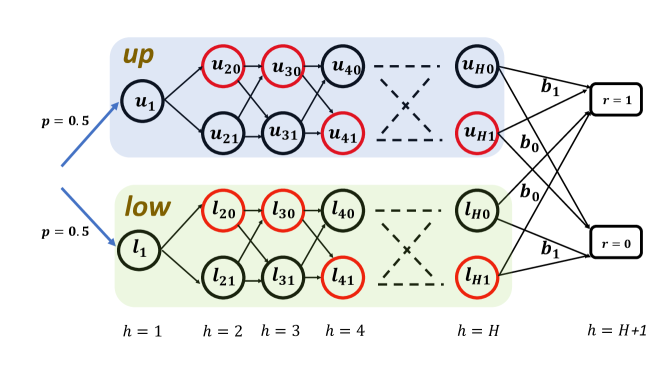
Figure 1: hard instance for Theorem 11.

The hard instance is best illustrated by Figure 1 where we sketch the transition dynamics of the POMG. Below we elaborate the construction based on Figure 1.

• States and actions. Each circle and rectangle in Figure 1 represents a state. Each player has two actions denoted by $\mathcal{A}=\{a_{0},a_{1}\}$ and $\mathcal{B}=\{b_{0},b_{1}\}$ respectively.

• Observations. The max-player can always directly observe the current latent state. The min-player observes the same dummy observation $o_{\rm null}$ in any black circle while directly observes the current state in any red circle and any rectangle. It is easy to verify by definition $\min_{h}\sigma_{\min}(\mathbb{O}_{h})=1$ because the emission structure is a bijection between the joint observation space and the latent state space.

• Reward. Only the upper rectangle emits an observation containing reward $1$ for the max-player (thus reward $-1$ for the min-player). All other states emit observations with zero reward.

• Transitions. At the beginning of each episode, the environment starts from $u_{1}$ or $l_{1}$ uniformly at random. The transition dynamics from step $1$ to step $H$ only depend on the actions of the max-player while in the final step ($H\rightarrow H+1$) the transitions are determined by the min-player. Formally,

  • When the environment is in the upper half of the POMG: for each step $h\in[H-1]$, the environment will transition to $u_{h+1,0}$ if the max-player takes action $a_{0}$ and transition to $u_{h+1,1}$ if the max-player takes action $a_{1}$. At step $H$, the agent will transition to the upper rectangle if the min-player takes action $b_{1}$ and transition to the lower one if the min-player picks $b_{0}$.

  • When the environment is in the lower half of the POMG: for each step $h\in[H-1]$, the environment will transition to $l_{h+1,0}$ if the max-player takes action $a_{0}$ and transition to $l_{h+1,1}$ if the max-player takes action $a_{1}$. At step $H$, the agent will transition to the upper rectangle if the min-player takes action $b_{0}$ and transition to the lower one if the min-player picks $b_{1}$.

Min-player’s optimal strategy.

It is direct to see the min-player’s optimal strategy is to take action $b_{0}$ in the upper half of the POMG and action $b_{1}$ in the lower half, at step $H$. This stratety will lead to zero-reward for the max-player. However, implementing this strategy requires the min-player to infer which half the environment is in from her observations, which is possible only when the environment has visited some red circles in the first $H$ steps. This is because the min-player directly observes the current state in red circles while observes the same observation $o_{\rm null}$ in all black circles.

Max-player’s optimal strategy.

To prevent the min-player from discovering which half the environment currently lies in, the max-player’s optimal strategy is to avoid visiting any red circles.

Hardness.

However, hardness happens if (a) the max-player cannot access the observations of the min-player and (b) for each $h\in\{2,\ldots,H\}$, we uniformly at random pick one of $\{u_{h0},u_{h1}\}$ and one of $\{l_{h0},l_{h1}\}$ to be red circles, and set the remaining ones to be black. From the perspective of the max-player, she cannot directly tell which state is red or black because (a) the difference between black circles and red circles only appear in the min-player’s observations, and (b) the max-player cannot see what the min-player observes. As a result, the only useful information for the max-player to figure out which circles are red is the action picked by the min-player in the final step.

Now suppose the min-player will play the optimal strategy when she knows which half the environment is in, and pick action $b_{0}$ when she does not. In this case, for the max-player, identifying all the red circles is as hard as learning a bandit with $\Omega(2^{H})$ arms where only one arm has reward $1/2$ and all other arms has reward $0$. Therefore, by using standard lower bound arguments for bandits, we can show the max-player’s cumulative rewards in the first $K=\Theta(2^{H})$ episodes is $0$ with constant probability. In comparison, the optimal strategy, which avoids visiting all red circles, can collect $K/3$ rewards with high probability. As a result, we obtain the desired $\Omega(\min\{2^{H},K\})$ regret lower bound for competing against the Nash value.

D.3 Playing against adversary in multi-step weakly-revealing POMGs is hard

In this section, we prove that competing with the max-min value is statistically hard even if (i) the POMG is two-player zero-sum and satisfies Assumption 2 with $m=2$ and $\alpha=1$, (ii) the opponent keeps playing a fixed action, and (iii) the player can directly observe the opponents’ actions and observations.

Theorem 24.

Assume the player can directly observe the opponents’ actions and observations. For any $L,k\in\mathbb{N}^{+}$, there exist (i) a two-player zero-sum POMG of size $S,A,O,H=\mathcal{O}(L)$ and satisfying Assumption 2 with $m=2$ and $\alpha=1$, and (ii) an opponent who keeps playing a fixed action $\hat{a}_{2}$, so that with probability at least $1/2$

$$\textstyle\sum_{t=1}^{k}\left(\max_{\tilde{\pi}_{1}}\min_{\tilde{\pi}_{2}}V_{1}^{\tilde{\pi}_{1}\times\tilde{\pi}_{2}}-V_{1}^{\pi^{t}_{1}\times\hat{a}_{2}}\right)\geq\Omega\left(\min\{2^{L},k\}\right),$$

where $\pi_{1}^{t}$ is the policy played by the learner in the $t^{\rm th}$ episode.

Proof.

The hard instance is constructed as following:

• States and actions: There are four states: $p_{0},p_{1}$ and $q_{0},q_{1}$. Each player has two actions, denoted by $\{a_{0},a_{1}\}$ and $\{b_{0},b_{1}\}$ respectively.

• Emission and reward: There are three different observations: $o_{\rm dummy}$, $o_{1}$ and $o_{0}$. At step $h\in[H-1]$, $p_{1}$ and $p_{0}$ emit the same observation $o_{\rm dummy}$. At step $H$, $p_{1}$ emits $o_{1}$ while $p_{0}$ emits $o_{0}$. Regardless of $h$, $q_{0}$ always emits $o_{0}$ and $q_{1}$ always emits $o_{1}$. Importantly, all players share the same observation. The reward function is defined so that $r(o_{\rm dummy})=r(o_{0})=0$ and $r(o_{1})=1$ for the max-player. Since the game is zero-sum, the reward function for the min-player is simply $-r(\cdot)$.

• Transition: Let $x_{1},\ldots,x_{h}$ be a binary sequence sampled independently and uniformly at random from standard Bernoulli distribution. At step $h=1$, the POMG always starts from state $p_{1}$. For each step $h\in[H-1]$:

  • If the current state is $p_{i}$, then the environment will transition to $p_{1}$ if and only if $i=1$, the max-player plays action $a_{x_{h}}$, and the min-player plays $b_{0}$. Otherwise, if the min-player plays $b_{1}$, then the environment will transition to $q_{i}$. Otherwise, the environment will transition to $p_{0}$.

  • If the current state is $q_{i}$, the next state will be $q_{1}$ regardless of players’ actions.

We have the following observations:

• If the min-player keeps playing $b_{0}$, then from the perspective of the max-player the POMG essentially reduces to a multi-arm bandit problem with $2^{H-1}$ arms because in this case the only useful feedback for the max-player is the reward observed at step $H$.

• The max-min (Nash) value is equal to $1$, which is attained when the max-player picks $a_{x_{h}}$ at step $h$ with probability $1$.

• The $2$-step emission-action matrix at each step $h\in[H-1]$ is rank $4$ and has minimum singular value no smaller than $1$, because we can always exactly identify the current state (for step $h\in[H-1]$) by the current-step observation and the next-step observation if the min-player picks action $b_{1}$ in the current step.

Based on the first two observations above, we immediately obtain a $\Theta(\min\{2^{H},k\})$ lower bound for competing with the max-min (Nash) value. Using the third observation, we know the POMG is $2$-step weakly revealing with $\alpha=1$, which completes the proof. ∎

References

- Brown and Sandholm (2019) Noam Brown and Tuomas Sandholm. Superhuman AI for multiplayer poker. Science, 365(6456):885–890, 2019.
- Vinyals et al. (2019) Oriol Vinyals, Igor Babuschkin, Wojciech M Czarnecki, Michael Mathieu, Andrew Dudzik, Junyoung Chung, David H Choi, Richard Powell, Timo Ewalds, Petko Georgiev, et al. Grandmaster level in StarCraft II using multi-agent reinforcement learning. Nature, 575(7782):350–354, 2019.
- Berner et al. (2019) Christopher Berner, Greg Brockman, Brooke Chan, Vicki Cheung, Przemyslaw Dkebiak, Christy Dennison, David Farhi, Quirin Fischer, Shariq Hashme, Chris Hesse, et al. Dota 2 with large scale deep reinforcement learning. arXiv preprint arXiv:1912.06680, 2019.
- Shalev-Shwartz et al. (2016) Shai Shalev-Shwartz, Shaked Shammah, and Amnon Shashua. Safe, multi-agent, reinforcement learning for autonomous driving. arXiv preprint arXiv:1610.03295, 2016.
- Papadimitriou and Tsitsiklis (1987) Christos H Papadimitriou and John N Tsitsiklis. The complexity of Markov decision processes. Mathematics of operations research, 12(3):441–450, 1987.
- Mundhenk et al. (2000) Martin Mundhenk, Judy Goldsmith, Christopher Lusena, and Eric Allender. Complexity of finite-horizon Markov decision process problems. Journal of the ACM (JACM), 47(4):681–720, 2000.
- Vlassis et al. (2012) Nikos Vlassis, Michael L Littman, and David Barber. On the computational complexity of stochastic controller optimization in POMDPs. ACM Transactions on Computation Theory (TOCT), 4(4):1–8, 2012.
- Mossel and Roch (2005) Elchanan Mossel and Sébastien Roch. Learning nonsingular phylogenies and hidden Markov models. In Proceedings of the thirty-seventh annual ACM symposium on Theory of computing, pages 366–375, 2005.
- Zinkevich et al. (2007) Martin Zinkevich, Michael Johanson, Michael Bowling, and Carmelo Piccione. Regret minimization in games with incomplete information. Advances in neural information processing systems, 20:1729–1736, 2007.
- Gordon (2007) Geoffrey J Gordon. No-regret algorithms for online convex programs. In Advances in Neural Information Processing Systems, pages 489–496. Citeseer, 2007.
- Farina and Sandholm (2021) Gabriele Farina and Tuomas Sandholm. Model-free online learning in unknown sequential decision making problems and games. arXiv preprint arXiv:2103.04539, 2021.
- Kozuno et al. (2021) Tadashi Kozuno, Pierre Ménard, Rémi Munos, and Michal Valko. Model-free learning for two-player zero-sum partially observable Markov games with perfect recall. arXiv preprint arXiv:2106.06279, 2021.
- Shapley (1953) Lloyd S Shapley. Stochastic games. Proceedings of the national academy of sciences, 39(10):1095–1100, 1953.
- Liu et al. (2022a) Qinghua Liu, Alan Chung, Csaba Szepesvari, and Chi Jin. When is partially observable reinforcement learning not scary? arXiv preprint, 2022a.
- Azar et al. (2017) Mohammad Gheshlaghi Azar, Ian Osband, and Rémi Munos. Minimax regret bounds for reinforcement learning. In International Conference on Machine Learning, pages 263–272. PMLR, 2017.
- Dann et al. (2017) Christoph Dann, Tor Lattimore, and Emma Brunskill. Unifying PAC and regret: Uniform PAC bounds for episodic reinforcement learning. Advances in Neural Information Processing Systems, 30, 2017.
- Jin et al. (2018) Chi Jin, Zeyuan Allen-Zhu, Sebastien Bubeck, and Michael I Jordan. Is Q-learning provably efficient? Advances in neural information processing systems, 31, 2018.
- Jin et al. (2020a) Chi Jin, Zhuoran Yang, Zhaoran Wang, and Michael I Jordan. Provably efficient reinforcement learning with linear function approximation. In Conference on Learning Theory, pages 2137–2143. PMLR, 2020a.
- Zanette et al. (2020) Andrea Zanette, Alessandro Lazaric, Mykel Kochenderfer, and Emma Brunskill. Learning near optimal policies with low inherent Bellman error. In International Conference on Machine Learning, pages 10978–10989. PMLR, 2020.
- Jiang et al. (2017) Nan Jiang, Akshay Krishnamurthy, Alekh Agarwal, John Langford, and Robert E Schapire. Contextual decision processes with low Bellman rank are PAC-learnable. In International Conference on Machine Learning, pages 1704–1713. PMLR, 2017.
- Jin et al. (2021a) Chi Jin, Qinghua Liu, and Sobhan Miryoosefi. Bellman eluder dimension: New rich classes of RL problems, and sample-efficient algorithms. Advances in Neural Information Processing Systems, 34, 2021a.
- Brafman and Tennenholtz (2002) Ronen I Brafman and Moshe Tennenholtz. R-max-a general polynomial time algorithm for near-optimal reinforcement learning. Journal of Machine Learning Research, 3(Oct):213–231, 2002.
- Wei et al. (2017) Chen-Yu Wei, Yi-Te Hong, and Chi-Jen Lu. Online reinforcement learning in stochastic games. In Advances in Neural Information Processing Systems, pages 4987–4997, 2017.
- Bai and Jin (2020) Yu Bai and Chi Jin. Provable self-play algorithms for competitive reinforcement learning. arXiv preprint arXiv:2002.04017, 2020.
- Liu et al. (2021) Qinghua Liu, Tiancheng Yu, Yu Bai, and Chi Jin. A sharp analysis of model-based reinforcement learning with self-play. In International Conference on Machine Learning, pages 7001–7010. PMLR, 2021.
- Bai et al. (2020) Yu Bai, Chi Jin, and Tiancheng Yu. Near-optimal reinforcement learning with self-play. In Advances in Neural Information Processing Systems, 2020.
- Xie et al. (2020) Qiaomin Xie, Yudong Chen, Zhaoran Wang, and Zhuoran Yang. Learning zero-sum simultaneous-move markov games using function approximation and correlated equilibrium. arXiv preprint arXiv:2002.07066, 2020.
- Jin et al. (2021b) Chi Jin, Qinghua Liu, and Tiancheng Yu. The power of exploiter: Provable multi-agent rl in large state spaces. arXiv preprint arXiv:2106.03352, 2021b.
- Jin et al. (2021c) Chi Jin, Qinghua Liu, Yuanhao Wang, and Tiancheng Yu. V-learning–a simple, efficient, decentralized algorithm for multiagent RL. arXiv preprint arXiv:2110.14555, 2021c.
- Song et al. (2021) Ziang Song, Song Mei, and Yu Bai. When can we learn general-sum markov games with a large number of players sample-efficiently? arXiv preprint arXiv:2110.04184, 2021.
- Daskalakis et al. (2022) Constantinos Daskalakis, Noah Golowich, and Kaiqing Zhang. The complexity of markov equilibrium in stochastic games. arXiv preprint arXiv:2204.03991, 2022.
- Krishnamurthy et al. (2016) Akshay Krishnamurthy, Alekh Agarwal, and John Langford. PAC reinforcement learning with rich observations. Advances in Neural Information Processing Systems, 29, 2016.
- Guo et al. (2016) Zhaohan Daniel Guo, Shayan Doroudi, and Emma Brunskill. A PAC RL algorithm for episodic POMDPs. In Artificial Intelligence and Statistics, pages 510–518. PMLR, 2016.
- Azizzadenesheli et al. (2016) Kamyar Azizzadenesheli, Alessandro Lazaric, and Animashree Anandkumar. Reinforcement learning of POMDPs using spectral methods. In Conference on Learning Theory, pages 193–256. PMLR, 2016.
- Jin et al. (2020b) Chi Jin, Sham M Kakade, Akshay Krishnamurthy, and Qinghua Liu. Sample-efficient reinforcement learning of undercomplete POMDPs. NeurIPS, 2020b.
- Farina et al. (2020) Gabriele Farina, Christian Kroer, and Tuomas Sandholm. Faster game solving via predictive Blackwell approachability: Connecting regret matching and mirror descent. arXiv preprint arXiv:2007.14358, 2020.
- Oliehoek (2012) Frans A Oliehoek. Decentralized pomdps. In Reinforcement Learning, pages 471–503. Springer, 2012.
- Oliehoek and Amato (2016) Frans A Oliehoek and Christopher Amato. A concise introduction to decentralized POMDPs. Springer, 2016.
- Nair et al. (2003) Ranjit Nair, Milind Tambe, Makoto Yokoo, David Pynadath, and Stacy Marsella. Taming decentralized pomdps: Towards efficient policy computation for multiagent settings. In IJCAI, volume 3, pages 705–711. Citeseer, 2003.
- Bernstein et al. (2005) Daniel S Bernstein, Eric A Hansen, and Shlomo Zilberstein. Bounded policy iteration for decentralized pomdps. In Proceedings of the nineteenth international joint conference on artificial intelligence (IJCAI), pages 52–57, 2005.
- Oliehoek et al. (2008) Frans A Oliehoek, Matthijs TJ Spaan, and Nikos Vlassis. Optimal and approximate q-value functions for decentralized pomdps. Journal of Artificial Intelligence Research, 32:289–353, 2008.
- Szer et al. (2012) Daniel Szer, François Charpillet, and Shlomo Zilberstein. Maa*: A heuristic search algorithm for solving decentralized pomdps. arXiv preprint arXiv:1207.1359, 2012.
- (43) Jilles Steeve Dibangoye, Christopher Amato, Olivier Buffet, and François Charpillet. Optimally solving dec-pomdps as continuous-state mdps. Journal of Artificial Intelligence Research, 55:443–497.
- Liu et al. (2017) Miao Liu, Kavinayan Sivakumar, Shayegan Omidshafiei, Christopher Amato, and Jonathan P How. Learning for multi-robot cooperation in partially observable stochastic environments with macro-actions. In 2017 IEEE/RSJ International Conference on Intelligent Robots and Systems (IROS), pages 1853–1860. IEEE, 2017.
- Amato et al. (2019) Christopher Amato, George Konidaris, Leslie P Kaelbling, and Jonathan P How. Modeling and planning with macro-actions in decentralized pomdps. Journal of Artificial Intelligence Research, 64:817–859, 2019.
- Gmytrasiewicz and Doshi (2005) Piotr J Gmytrasiewicz and Prashant Doshi. A framework for sequential planning in multi-agent settings. Journal of Artificial Intelligence Research, 24:49–79, 2005.
- Doshi et al. (2009) Prashant Doshi, Yifeng Zeng, and Qiongyu Chen. Graphical models for interactive pomdps: representations and solutions. Autonomous Agents and Multi-Agent Systems, 18(3):376–416, 2009.
- Liu et al. (2022b) Qinghua Liu, Yuanhao Wang, and Chi Jin. Learning markov games with adversarial opponents: Efficient algorithms and fundamental limits. arXiv preprint arXiv:2203.06803, 2022b.
- Jakobsen et al. (2016) Sune K Jakobsen, Troels B Srensen, and Vincent Conitzer. Timeability of extensive-form games. In Proceedings of the 2016 ACM Conference on Innovations in Theoretical Computer Science, pages 191–199, 2016.
- Bai et al. (2022) Yu Bai, Chi Jin, Song Mei, and Tiancheng Yu. Near-optimal learning of extensive-form games with imperfect information. arXiv preprint arXiv:2202.01752, 2022.