Ice friction at the nanoscale

Abstract

The origin of ice slipperiness has been a matter of great controversy for more than a century, but an atomistic understanding of ice friction is still lacking. Here, we perform computer simulations of an atomically smooth substrate sliding on ice. In a large temperature range between 230 and 266 K, hydrophobic sliders exhibit a premelting layer similar to that found at the ice/air interface. On the contrary, hydrophilic sliders show larger premelting and a strong increase of the first adsorption layer. The non-equilibrium simulations show that premelting films of barely one nanometer thickness are sufficient to provide a lubricating quasi-liquid layer with rheological properties similar to bulk undercooled water. Upon shearing, the films display a pattern consistent with lubricating Couette flow, but the boundary conditions at the wall vary strongly with substrate’s interactions. Hydrophobic walls exhibit large slip, while hydrophilic walls obey stick boundary conditions with small negative slip. By compressing ice above atmospheric pressure, the lubricating layer grows continuously, and the rheological properties approach bulk–like behavior. Below 260 K, the equilibrium premelting films decrease significantly. However, a very large slip persists on the hydrophobic walls, while the increased friction on hydrophilic walls is sufficient to melt ice and create a lubrication layer in a few nanoseconds. Our results show the atomic scale frictional behavior of ice is a combination of spontaneous premelting, pressure melting and frictional heating.

The slipperiness of ice has been exploited since ancient times as a means of transportation in cold regions [1].

But despite many advances on tribology [2, 3, 4] a first principles understanding on this very familiar property is still lacking [5].

A hypothesis dating back to the 19th century is that a self-lubricating water film on the ice surface is formed due to pressure melting [6, 7]. Spontaneous equilibrium premelting [8], and frictional heating [9], have also been invoked to explain ice friction. However, other authors disregard the significance of water lubrication altogether [10, 11, 12, 13], while recent experiments support boundary or elastohydrodynamic models of friction [12, 14, 13, 15]. Experimental confirmation of interfacial premelting films in the order of the nanometer does not resolve the controversy [16, 17, 18, 19, 20, 21], as it is arguable whether macroscopic hydrodynamics assumed in most theories [22, 23, 24] is obeyed at such small length-scales [25]. In fact, computer simulations of flow under confinement reveal consistent violation of the stick boundary condition and the significance of water slip [26, 27, 28, 29, 30], while studies of water sliding on ice and grain boundary friction suggest negative slip instead [31, 32].

Here we report Molecular Dynamics simulations of ice sliding past an atomically smooth substrate. Our results show that an interfacial premelting film formed spontaneously upon compression or frictional heating, exhibits hydrodynamic properties similar to bulk undercooled water. This illustrates that a hydrodynamic theory of Couette flow supplemented with slip boundary conditions can explain the friction of ice at smooth contacts.

Results

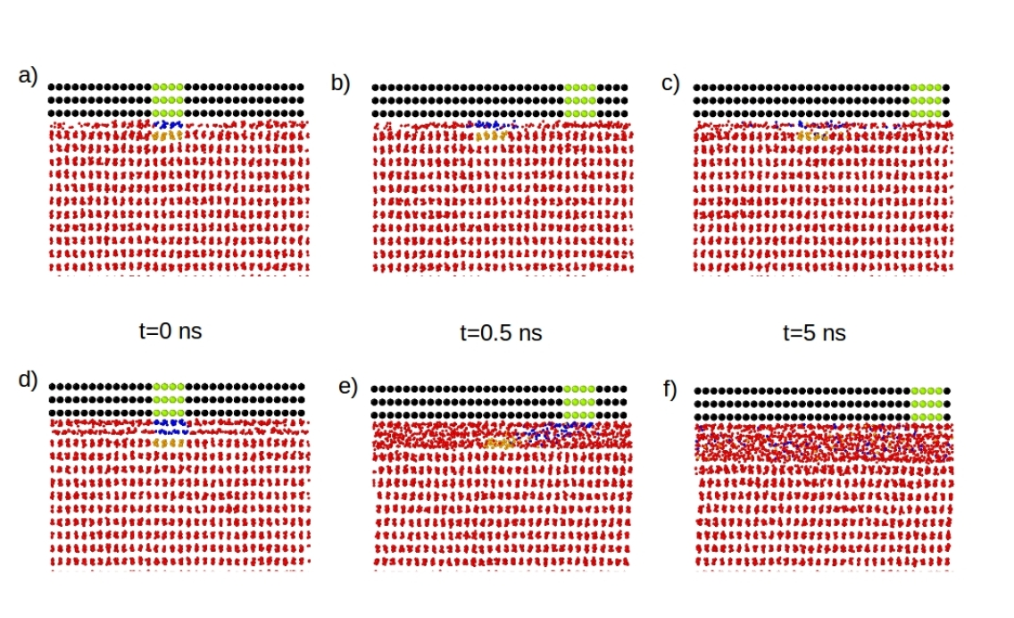
Figure 1: Time sequence of a shearing experiment at $T=230$ K. (a-c) A hydrophobic slider ($\theta=120^{\circ}$) barely one nanometer thick slips past the substrate. (d-f) A hydrophilic slider ($\theta=50^{\circ}$) sticks to the substrate and exhibits significant frictional melting. Color codes as in Figure 1 of main text.

In our study, we simulate explicitly ice sliding past an atomically smooth substrate under pressure (Fig. 1). The ice sample consists of a large orthorombic slab of water molecules (30 bilayers thick) modeled with the TIP4P/Ice force field and oriented in the direction of the basal surface [33]. The slider is modeled as a rigid face–centered cubic arrangement of atoms directed along the (111) plane, with lattice parameters selected to make a perfect match with the ice surface.

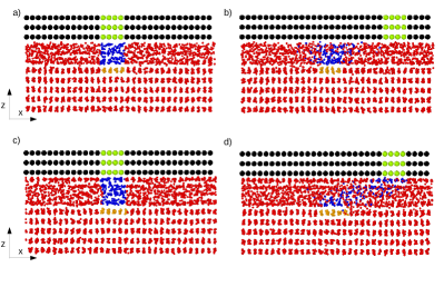
Figure 1: Sliding on ice with atomic resolution. An imperfectly terminated ice slab gently compressed to $p=1$ atm by an inert solid substrate at T=262 K spontaneously develops a premelting film of thickness ca. $h=1$ nm for both hydrophobic (a) and hydrophilic walls (c). The flow pattern after sliding over the equilibrated film with sliding velocity $U=5$ m$/$s during 0.5 ns is illustrated by liquid-like molecules tagged in blue and wall atoms tagged in green color at $t=0$. (b) For the hydrophobic substrate, the slider slips past the premelting film, and the liquid-like blue tagged molecules have hardly moved beyond their original position at $t=0$ (see also Movie S1). (d) For the hydrophilic substrate, an adsorption layer sticks to the wall and the premelting film is dragged by the slider with a pattern that resembles Couette flow (see also Supplementary Movie 2). Solid like orange colored molecules serve to illustrate stick boundary conditions at the ice/water interface and the exchange of solid and liquid molecules.

The wall atoms interact with water oxygens via a Lennard-Jones potential. This allows us to tune the hydrophobicity of the substrate merely by changing the strength of wall-oxygen interactions. The quality of the substrate is monitored by measuring the contact angle of water droplets, $\theta$, which is varied in a range spaning both hydrophobic ($\theta=120^{\circ}$) and hydrophilic ($\theta=50^{\circ}$) walls (SI Appendix Text and Methods).

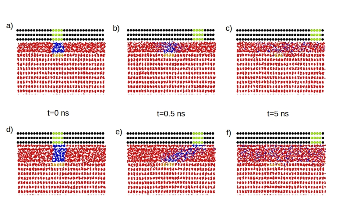
Figure 2: Time sequence of a shearing experiment at $T=266$ K. (a-c) The hydrophobic slider ($\theta=120^{\circ}$) slips. (d-f) The hydrophilic slider ($\theta=50^{\circ}$) sticks. Color code as in Figure 1 of main text.

Under skating conditions, the slider does not step on a perfectly terminated ice surface. Instead, the ice surface has been previously exposed to air, and exhibits a significant premelting layer [34, 31, 35, 36]. To mimic the contact of the slider with ice, we merely prepare the ice surface with a half terminated bilayer and place it at a small distance from the substrate. The wall is then allowed to gently compress the slab to the desired pressure (see Methods Section). At a temperature $T=262$ K, somewhat lower but close to that of skating rinks, we find that a premelting film of the order of a nanometer thick evolves spontaneously and equilibrates in the scale of decades of nanoseconds for all substrates and pressures studied. The presence of premelting is obvious in the snapshots of Fig. 1 as a layer of disordered water molecules between the ordered bulk ice and the substrate. In the density profiles of Fig. 2-a,b,c,d, the signature of premelting is the emergence of density peaks that have lost the bilayer structure typical of bulk ice that is apparent within the bulk region. This is confirmed by use of the CHILL+ order parameter [37], which allows to resolve solid-like from liquid-like water molecules (SI Appendix Methods).

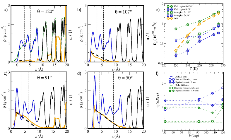
Figure 2: Structure and dynamics of premelted films during sliding. Panels (a,b,c,d) show equilibrium density profiles and velocity profiles for a a sliding experiment at $p=1$ atm, $T=262$ K and $U=5$ m$/s$ during 10 ns. The total density profile (left axis) is shown as a continuous line, with blue colour for the region where liquid-like water is the majority phase and black colour where ice is the majority phase. The premelting film is divided into a wall-adsorbed layer, an ice-adsorbed layer and a central quasi-bulk region, as illustrated by vertical dashed lines. Panel (a) also shows the total density of a premelting film for ice in contact with vacuum (green dashed line). The thick orange lines display the velocity profile in units of the sliding velocity (right axis, with tick marks as displayed in the left axis). The dashed black line is the hydrodynamic flow profile predicted from the model of Eq. (1). Panels correspond to different wall interactions (a) Hydrophobic wall, with $\theta=120^{\circ}$ (b) $\theta=107^{\circ}$ (c) $\theta=91^{\circ}$ (d) Hydrophilic wall with $\theta=50^{\circ}$. Panel (e): Diffusivity at the wall and ice adsorption layers as a function of temperature. The orange diamonds stand for the bulk diffusion coefficients at $p=1$ atm. The remaining symbols correspond to parallel diffusion coefficients of the wall-adsorption layer (circles) and the ice-Adsorption layer (squares); Green symbols stand for the hydrophobic wall with $\theta=120^{\circ}$ and blue symbols for the hydrophilic wall with $\theta=50^{\circ}$. Panel (f): Quasi-bulk like viscosity of the premelting film. The thick dashed line displays the shear viscosity of bulk undercooled water as determined from Green-Kubo calculations. The circles display viscosities as determined from the Stokes-Einstein relation using the parallel diffusion coefficient calculated in the central quasi-bulk like region of the premelting films. The diamonds are hydrodynamic viscosities as determined from the film thickness and shear stress of the simulations. Results are shown for $T=262$ K, with $p=1$ atm (blue) and $p=600$ atm (green).

After equilibration, we model sliding by moving the top and bottom sliders with equal sliding speed $U=5$ m$/$s and opposite direction. Although the properties of premelting layers of ice exposed to vacuum are often invoked as a proxy to explain ice friction [5, 31, 12], inspection of simulation snapshots show a dramatic dependence of the sliding dynamics on the substrate interactions. Here we describe results obtained at ambient pressure $p=1$ atm and $T=262$ K (Fig. 1 and movies S1 and S2), but similar results are found in all the temperature range from 230 to 266 K (c.f. SI Appendix, Fig. S1 and S2).

For the hydrophobic substrate, $\theta=120^{\circ}$, the slider slips past the premelting film, and generates an extremely small velocity field. Molecules tagged in blue in Fig. 1-(a) at $t=0$ have diffused almost equally in both directions after a sliding time of 0.5 ns (Fig. 1-(b)). i.e.: as observed in the flow of water inside carbon nanotubes [26, 28, 38, 30], friction is extremely small, and the premelting film is hardly susceptible to the motion of the slider. On the contrary, for the hydrophilic substrate, with $\theta=50^{\circ}$, an adsorbed layer of water molecules next to the substrate at $t=0$ (Fig. 1-(c)) sticks to the wall and is displaced by the same amount as the slider after 0.5 ns (Fig. 1-(d)). The remaining blue tagged molecules in the premelting film are loosely dragged by the slider and display clear hints of Couette flow.

The large difference in the frictional behavior can be anticipated from the plot of equilibrium density profiles [39]. Here we describe results obtained at T=262 K (Fig. 2-(a,b,c,d)), but the same trend is observed in all the temperature range studied (SI Appendix Fig, S3 and S4). For the hydrophobic substrate ($\theta=120^{\circ}$) the structure of the premelting film is very similar to that found when the ice surface is exposed to vacuum (green dashed line in Fig. 2-(a)). The density profiles differ significantly only by the presence of a small density peak that appears in the confined film close to the wall. However, increasing the strength of the wall interactions results in an increase of the film thickness and the appearance of a strongly layered liquid film. Particularly, we see a large enhancement of the first adsorption peak, with a density that can increase as much as a factor of three compared to that observed in the hydrophobic wall with $\theta=120^{\circ}$ (Fig. 2-(d)). By visual inspection we confirm that the water molecules pertaining to the first adsorption peak exhibit strong intra-layer hydrogen bonding, with proliferation of flattened hexagonal rings as observed in adsorbed thin films on metals [40, 41], and undercooled water under confinement [42, 43].

We expect the hydrogen bond network on the first adsorption peak of hydrophilic substrates to have a significant impact on the mobility of water molecules [31, 34, 39]. To show this, we divide the premelting film into regions that allow us to single out the wall adsorption layer from the ice adsorption layer, as illustrated with vertical dashed lines in Fig. 2-(a,b,c,d)). For each of these two regions, we estimate an effective parallel self-diffusion coefficient, $D_{\parallel}$ by measuring the tangential mean squared displacement of the water like molecules in that region (Fig. 2-(e)). Our results confirm a dramatic impact of the wall-water interactions on the mobility of the wall-adsorption layer. For the hydrophobic substrate, $\theta=120^{\circ}$, the parallel diffusion coefficient is somewhat larger than that of bulk undercooled water for most temperatures studied, as observed in premelting films exposed to vacuum [12, 31, 34], and becomes an order of magnitude larger on approaching 230 K. However, for the hydrophilic substrate, $\theta=50^{\circ}$, the diffusion coefficient of the wall adsorption layer remains one order of magnitude smaller than that of the hydrophobic substrate all the way from 266 to 230 K. On the other hand, for the ice-adsorption layer the diffusion coefficient remains small and almost independent of $\theta$, implying that the details of the slider do not impact the friction of premelted water at the ice interface.

For temperatures above 260 K, the premelting layer develops a well defined quasi-bulk region between the adsorption layers, as observed in Fig.2 and SI Appendix Figs. S3 and S4. Our results show that the parallel diffusion coefficient in this central region is somewhat smaller, but of the same order of magnitude as the diffusion coefficient of bulk water, even for the films studied here, which are barely 1 nm thick [26] (c.f. SI Appendix Fig. S5). This is in agreement with measurements of mobility in confined water [44, 26, 45, 21], and suggests that large effective viscosities measured in mechanical tests [14] might not be related to the actual hydrodynamics of the premelting film, as noticed in Ref. [21]. This is not in conflict with the observation of anomalous diffusion at grain boundaries, which is related to the attachment/detachment of water molecules into the ordered ice lattice due to motion in the perpendicular direction [46]. We find that in the time scale of about 2-8 ns in which premelted water molecules remain within the central quasi-bulk region of the premelting film, the mobility in the parallel direction remains close to bulk like. This suggests that the central region within the premelting film will exhibit shearing similar to that observed in bulk undercooled water. As a hint, we notice that the viscosity predicted from the Stokes-Einstein relation $\eta_{SE}=k_{B}T/6\pi D_{\parallel}a$, with $a=0.155$ nm describing the molecular radius of a water molecule provides an order of magnitude approximation to the viscosity of undercooled water calculated independently at $T=262$ K and $p=1$ atm from bulk simulations (Fig. 2-(f)).

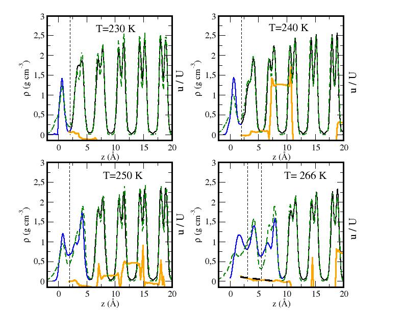
Figure 3: Structure and velocity flow of the premelted film. Results are shown for a hydrophobic slider ($\theta=120^{\circ}$) at $p=1$ atm in a range of temperatures. The equilibrium density profile in g cm^-3 (left axis) is shown as a continuous line, with blue colour for the region where liquid-like water is the majority phase and black colour where ice is the majority phase. Green dashed lines describe the total density profile at the ice/air interface (results from SI Appendix Ref.[14]). Vertical black dashed lines serve to separate adsorption layers next to the wall and bulk ice. An additional line separates a central quasi-bulk region where possible. The thick continuous lines display the velocity profile in units of the sliding velocity for a sliding experiment with $U=5$ m$/s$ during 10 ns (right axis). The dashed black line in the panel at T=266 K is the hydrodynamic flow profile predicted from the model of Eq. (1) in the main text. For lower temperatures the flow profile is too noisy to obtain any reliable information.

In practice, sliding occurs at contact with surface asperities, and the pressure on the contact zone can well reach several hundred atmospheres [9, 23, 24, 12, 13, 15]. However, increasing pressure drives ice closer to the melting line. Therefore, the thickness of the premelting film is expected to increase. We confirm this by compressing our confined ice slabs, and estimating the equilibrium film thickness as $h_{eq}=\Gamma_{w}/\rho_{w}$, with $\Gamma_{w}$, the number of liquid–like molecules per unit surface, and $\rho_{w}$ the bulk liquid density. The results of Fig. 3 show that, independent of the substrate quality, the interfacially premelted films increase their thickness under compression, showing that pressure melting and interfacial premelting are inextricably entangled [16, 18].

As a result of this surface-pressure melting, the diffusion coefficient and the corresponding Stokes-Einstein viscosity of the films approach bulk-like conditions as illustrated in SI Appendix Fig. S5 and Fig. 2-(f) for interfacially premelted films compressed at a pressure of $p=600$ atm.

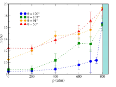
Figure 3: Increasing equilibrium premelting thickness by compression. Results display the equilibrium interfacial premelting thickness as a function of pressure for different substrates at $T=262$ K. Blue circles: $\theta=120^{\circ}$; Green squares: $\theta=107^{\circ}$; organge triangles: $\theta=91^{\circ}$; red triangles: $\theta=50^{\circ}$. The hashed region displays the estimated melting pressure for the model.

In order to check how bulk-like is the sliding hydrodynamics of a quasi-liquid layer barely one nanometer thick, we study the shear response of the premelting film upon sliding the wall with a constant lateral velocity $U=5$ m$/$s at T=262 K and $p=1$ atm for a period of 10 ns (Fig. 2-(a,b,c,d)). Similar calculations are performed for $p=600$ atm (SI Appendix Fig. S6) and $p=1$ atm in the temperature range 230 to 266 K (SI Appendix Figs. S3 and S7).

Averaging the velocity components in the $x$ direction parallel to the slider, we obtain the hydrodynamic flow profile $u(z)$ as a function of the perpendicular distance to the wall. For the hydrophobic wall (Fig. 2-(a)), $u(z)$ is hardly distinguishable from thermal motion [28]. It appears as a noisy curve with very small positive velocity that hardly attains 10% of the total wall velocity. However, as the wall hydrophilicity begins to increase (Fig. 2-(b,c,d)), a roughly linear flow profile appears that strongly resembles expectations from a model of simple Couette flow with partial slip [47, 48, 2, 28, 38]. By visual inspection we can define $\sigma_{1}$ as the position close to the wall adsorption peak where the approximately linear flow profile attains its maximal velocity, $u_{s}=u(z=\sigma_{1})$. Similarly, we define $\sigma_{2}$, close to the ice adsorption peak, where the extrapolated flow profile vanishes, $u(z=\sigma_{2})=0$ (See SI Appendix Fig. S8, and Tables S1 and S2). Interestingly, we find $\sigma_{2}$ is at about one molecular diameter away from the first ice bilayer, in agreement with reports of a small negative slip length for water flow past bulk ice [49].

If the hydrodynamics of the premelting film follows a model of Couette flow, we expect the shear stress, $\tau$, should obey $\tau=\eta\frac{u_{s}}{d_{C}}$,[2, 3, 48] where $u_{s}$ is the slip velocity, $u_{s}=u(z=\sigma_{1})$, $d_{C}$ is the thickness of the region where the actual Couette flow takes place and $\eta$ is the bulk viscosity. To check this, we calculate the effective hydrodynamic viscosity as $\eta_{H}=\tau d_{C}/u_{s}$, with $\tau$ measured from the force exerted by the wall on the premelting film, $d_{C}=\sigma_{2}-\sigma_{1}$ and $u_{s}$ estimated by visual inspection of the flow profile. The results for $\eta_{H}$ are shown in Fig. 2-(f), and appear barely 10% above the viscosity of bulk water. Alternatively, we can assume the premelting film behaves as bulk water and obtain a hydrodynamic film thickness as $d_{H}=\eta u_{s}/\tau$, with $\eta$ the bulk viscosity [38]. We checked that the value thus obtained agrees within $\pm 0.3$ nm with the estimated Couette thickness, $d_{C}$. Now, using $d_{H}$, and $u_{s}$ we can obtain a synthetic Couette flow profile under the assumption that $u(z)=u_{s}$ at $z=\sigma_{1}$ and vanishes at $z=\sigma_{1}+d_{H}$. The resulting model is displayed in Fig. 2-(a,b,c,d) together with the actual velocity profiles measured in the simulations. A qualitative agreement is obvious for substrates $\theta=107^{\circ}$ and $\theta=91^{\circ}$, and is almost as good as a linear regression for the hydrophilic substrate with $\theta=50^{\circ}$ (similar good agreement is found also for $p=600$ atm, c.f. SI Appendix Fig.S6 and $T=266$ K, SI Appendix Fig.S3 and S7). As a rule of thumb, we see that the Couette flow is established between the wall and ice adsorption layers of liquid–like water, so that the location of the hydrodynamic boundary conditions may be inferred with little cost from equilibrium simulations.

Put together, our results strongly support that the shear force of the slider on thin premelting films hardly one nanometer thick may be described approximately by a very simple model of Couette flow with slip:

$$\tau=\displaystyle\frac{\eta\,U}{h_{H}+b}$$ (1)

where $h_{H}=\sigma_{1}+d_{H}$ is the hydrodynamic film thickness, $b$ is a slip length and $\eta$ is an effective viscosity similar to the viscosity of undercooled bulk water (SI Appendix Fig. S8). We test the consistency of the model by performing additional simulations at a smaller sliding velocity $U=0.5$ m$/$s and find that the calculated shear force is about 10 times smaller than that measured at $U=5$ m/s, consistent with Eq. (1) (See SI Appendix Table S3).

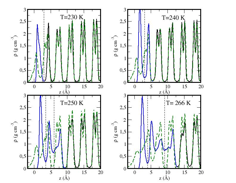
Figure 4: Structure and velocity flow of the premelted film. Results are shown for a hydrophilic slider ($\theta=50^{\circ}$) at $p=1$ atm in a range of temperatures. The equilibrium density profile in g cm^-3 (left axis) is shown as a continuous line, with blue colour for the region where liquid-like water is the majority phase and black colour where ice is the majority phase. Green dashed lines describe the total density profile at the ice/air interface (results from SI Appendix Ref.[14]). Vertical black dashed lines serve to separate adsorption layers next to the wall and bulk ice. An additional line separates a central quasi-bulk region where possible. Velocity profiles are not shown in this case because substantial frictional melting distorts the premelting film structure, but see Supplementary Figure 7.

We can estimate a Couette slip length $b_{C}$ for use in Eq. (1) directly from visual inspection of the velocity profile of Fig. 2-(a,b,c,d), noticing that $U/(d_{C}+\sigma_{1}+b_{C})=u_{s}/d_{C}$. A figure of the slip length as a function of wall strength illustrates the large difference of frictional behavior. For $\theta=120^{\circ}$, $b$ is about 5 times larger than the actual film thickness, consistent with observations of giant slip lengths in confined undercooled water and water at hydrophobic substrates [26, 30]. As the wall strength increases, however, the slip length decreases fast and becomes negative for hydrophilic walls, illustrating a large impact of wall interactions on the early stages of ice friction (Fig. 4).

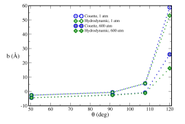
Figure 4: Slip and stick boundary conditions of premelted films. As wall hydrophilicity increases, the premelting film dynamics evolves from large to negative slip. Blue circles are Couette slip lengths, $b_{C}$ estimated from the average flow profile. Green diamonds are hydrodynamic slip lengths, $b_{H}$ calculated from the shear force.

To further check the consistency of the model, we can invoke the Navier slip boundary condition, which assumes a shear stress proportional to the velocity drop at the hydrodynamic boundary, i.e. $\tau=\lambda(U-u_{s})$, where $\lambda=\eta/b$ is the interfacial friction coefficient [48, 27, 28, 38]. Combining these equations, we estimate a hydrodynamic slip length $b_{H}=(U-u_{s})\eta/\tau$ by using the shear stress obtained in the simulations, $u_{s}$ from the velocity profile and $\eta$ the viscosity of bulk water. The results in Fig. 4 show remarkable good agreement with the Couette slip length measured previously and attests to the accuracy of Eq. (1) as a valid model for the shear stress of an atomically smooth sliders on ice.

Since increasing the temperature or pressure increases the equilibrium film thickness, Eq. (1) is expected to hold everywhere above T=262 K and $p=1$ atm. At lower temperature, however, Figs. S3 and S4 show that the premelting films consist of at most two adsorption layers and no quasi-bulk region at all. This drives the system fully into the boundary friction regime. Surprisingly, the ice surface remains slippery both for hydrophobic and hydrophilic sliders. Indeed, using our results for the shear stress from the non-equilibrium simulations (SI Appendix Tables S3 and S4), and indentation hardness results for the applied load [13], we find order of magnitude agreement with experimental friction coefficients in all the temperature range studied (c.f. SI Appendix Text and Fig. S9). The origin of the small friction coefficients varies greatly with hydrophilicity, however. In the case of hydrophobic sliders, the diffusion coefficient of the adsorption layer remains always larger than the bulk diffusion coefficient (Fig.2-e), and allows for a very large slip (Fig. S1 and S2), as suggested in Ref.[12]. For hydrophilic sliders, on the contrary, shear is sufficiently large to melt one full bilayer in barely 0.5 ns due to frictional heating. As a result, an equilibrium premelting film consisting of one single adsorption layer attains nanometer thickness in less than 5 ns (c.f. Fig.S1 and Movie M3).Therefore, hydrophilic sliders develop a layer that is sufficiently thick to achieve lubrication, even at low temperature. This is visible in the close to linear velocity profiles observed in Fig.S7. However, for a nanometer thick film at the large sliding speeds $U=5$ m/s that we study, the shear rate $\dot{\gamma}=U/d$ attains the scale of $5\cdot 10^{9}$ s^-1. Above 262 K this is still small and the lubrication layer exhibits Newtonian flow. However, as the temperature decreases, this becomes well above the threshold of non-Newtonian flow [50]. Indeed, from the velocity profiles of Fig.S7 we find hydrodynamic viscosities that become up to two orders of magnitude smaller than the bulk viscosity at T=230 K. The shear rate dependent viscosities so obtained roughly follow the Eyring model of shear thinning (c.f. SI Appendix Text and Fig. S10). Interestingly, the hydrophilic sliders at low temperature display a small elastic deformation (c.f. Movie S3), but this accounts only for a few percent of the total shear stress (c.f. SI Appendix Text).

Discussion

In practice, ice friction is a multiscale problem, and both the slider and ice are atomically rough [4, 51]. As a result, it is thought that most of the slider’s load is supported locally in high–pressure zones [9, 23, 24, 12, 13, 15]. In conventional applications, low viscosity liquids such as water behave as very poor lubricants, because the large pressure between asperities squeezes out the lubrication film, resulting in bare contact friction [23, 2, 3, 13, 15]. This argument was used recently by Canale et al.[14] and Bonn et al.[12, 13] to put into question the role of premelting mediated lubrication in ice friction. Our results show ice does not behave as an ordinary inert substrate. Increasing the pressure drives it closer to the melting line, and leads to an increase of the equilibrium premelting thickness (c.f. Fig.3). Of course, a high contact pressure will conspire to squeeze out the lubrication film [52]. By Le Chatelier’s principle, however, ice will melt in order to restore the equilibrium thickness [16, 18, 53]. Due to this self-healing property of the premelting film, we expect lubrication will be enhanced at high pressure.

Based on these considerations, and the model of Eq. (1), we find that the friction coefficient of an atomically smooth region on the ice/slider system should obey $\mu_{f}=\frac{\eta(\dot{\gamma})U}{(h_{H}+b)p}$, where $p$ is the pressure of the high pressure zone [23, 24].

At $T=262$ K, moderate sliding speeds of the order of mm/s, assumed film thicknesses of ca. 1 nm and zero slip, this gives already a small friction coefficients at a pressure of one atm, ca. $\mu_{f}=0.1$. Considering instead that the sliding contact is exercised at the indentation hardness limit of ca. $p=100$-$1000$ atm [11, 24, 12, 13], we obtain friction coefficients two to three orders of magnitude smaller. Increasing the sliding velocity to the m/s range yields higher estimates of order $\mu_{f}\approx 1$, well away from experimental measurements. However, at such ranges, friction inputs heat at a large rate of $\eta U^{2}/(h_{H}+b)$ ca. 35-200 MJ/m²s, which is sufficient to melt roughly one full bilayer in the scale of nanoseconds. Unless heat is dissipated within the slider at a very fast rate, this will result in a large increase of the film thickness within a few hundred nanoseconds, as assumed tacitly in current theories of frictional heating [23, 24]. Indeed, we can see in our 10 ns sliding simulations clear evidence of bilayer melting at temperatures as low as 230 K, despite the use of a thermostat (c.f. Movie S3).

Our model is also consistent with the temperature dependence observed for the friction coefficient [9, 10, 11, 12, 13]. For hydrophobic walls at low temperature, the slip length becomes very large [30], and the lubrication model with slip yields $\mu_{f}=\lambda U/p$, where $\lambda$ is the interfacial friction [48]. For undercooled water, $\lambda(T)$ follows an Anti-Arrhenius behavior[30] that is consistent with a large increase of $\mu_{f}$ with decreasing temperature [10, 11, 12, 13]. The result $\mu_{f}=\lambda U/p$ also explains the velocity strengthening observed for the friction coefficient at slow velocities [11, 54, 13]. At larger sliding velocities, shear thining becomes significant. This leads to a friction coefficient with a weaker, logarithmic dependence on the sliding speed, $\mu_{f}\propto\ln(U)/p$ (c.f. SI Appendix Text). When the pressure is equated to the indentation hardness, which increases faster than $\ln(U)$ [13], this results in the velocity weakening of the friction coefficient found in experiments [9, 10, 11, 54, 13].

Overall, we find our results lend strong support to the hypothesis of lubricated ice friction that has been put into question in recent experiments based on milimeter scale probes [12, 14, 13]. Contrary to findings by Canale et al.[14] for corrugated probes our results suggest that at atomically smooth contacts, the effective viscosity $\eta$ is a meaningfull and well defined parameter, on the order of the bulk viscosity, which exhibits shear thinning at low temperature. Unlike suggestions by Weber et al. [12], the dependence of ice friction on substrate’s slip length $b$ shows that the sliding dynamics cannot be generally correlated with the properties of premelting films at the ice/vapor interface, except for highly hydrophobic sliders.

We emphasize, however that our results describe the frictional behavior at atomically smooth contacts. At a larger scale, both the slider and ice exhibit microscale roughness, and the total load of the slider is supported by a small amount of asperities. Accordingly, the friction coefficient is not only given by the shear at the smooth contacts, but also, by the indentation hardness of ice, which sets the fractional area supporting the slider’s load [11, 24, 12, 13]. At a larger scale, the formation of a slurry of water and ice could result in a very complex visco-elastic response [14, 15].

In summary, we have shown that a very small extent of interfacial premelting in ice provides a lubricating quasi-liquid layer that can be described close to quantitatively by a model of bulk Couette flow with slip. The premelted layer can further grow by compression and frictional heating. Our results reconcile the long–standing controversy on the origin of ice slipperiness and show that equilibrium premelting, pressure melting and frictional heating operate simultaneously.

Methods

Computer simulations

Molecular Dynamics simulations on the Np_zAT ensemble were performed using LAMMPS [55]. Trajectories were evolved with the velocity-Verlet algorithm, with a time step of $2$ fs. Bonds and bond angles were constrained by the use of the SHAKE algorithm. The temperature was set using the velocity rescale algorithm with damping factor $\tau=0.2$ ps [56]. The pressure was set by applying a constant normal force $F_{z}=\pm p_{z}A/N_{w}$ directed in the direction of bulk ice on each of the $N_{w}$ wall atoms [38, 29, 30]. This avoids perturbation of the dynamics that is usual in conventional barostats. To prevent strain effects in the parallel direction, the lattice parameters are set to the equilibrium value at pressure $p_{z}$. Shear was imposed on ice by moving the walls tangentially in the $x$ direction at constant sliding speed (with opposite direction on each wall) [48, 2, 38, 32]. All Lennard-Jones interactions were truncated beyond 1 nm. Electrostatic interactions were evaluated with a particle-particle particle-mesh solver. The charge structure factors were evaluated with a grid spacing of $1$ Å and a fourth order interpolation scheme. It resulted in $36\times 32\times 120$ ($72\times 64\times 120$ during Couette flow simulations) vectors in the $x,y,z$ reciprocal directions, respectively. In the Non-Equilibrium simulations, equilibrated bulk systems were replicated by a factor of two on each of the parallel directions to gather sufficient statistics for the flow profile, and the thermostat was set only in the directions perpendicular to the flow, using a damping factor $\tau=1$ ps. Shear was imposed on ice by moving the walls tangentially in the $x$ direction at constant sliding speed for 10 ns (with opposite direction on each wall). The averages were collected over 10 independent runs. Further details on the simulation setup and analysis may be found in the SI Appendix Methods and Figs. S11-S15.

Data Availability

All the study data are included in the article and the supporting information.

Supporting Information for

Ice friction at the nanoscale
by
Łukasz Baran^a, Pablo Llombart^b, Wojciech Rżysko^a and Luis G. MacDowell

Choice of wall model

Notice we have chosen a generic model substrate with an FCC crystalline order. This choice is a matter of convenience, since the FCC lattice in the (111) direction can be made to match perfectly the hexagonal ice lattice in the basal direction (c.f. SI Appendix Methods). However, many metals such as Pt, Pd, and Ru exhibit close match with ice, c.f. Ref.(41), so the lattice geometry employed here is not unrealistic.

In practice, we set the value of the Lennard-Jones range parameter, $\sigma_{wo}=3.1668$ Å, equal to that of TIP4P/Ice water for convenience. This is somewhat larger than the usual values for metals (c.f. 2.55 Å for Cu and Fe), and somewhat smaller than those of CH2 and CH3 groups in united models of alkanes (ca. 3.9 Å and 3.7 Å for the OPLS or TraPPE models, SI Appendix Ref.[1, 2]). Therefore, our substrate is reasonable but does not particularly match any specific choice of material. However, by tuning the LJ energy parameter, $\epsilon_{wo}$, we tune the contact angles from 50 to 120 degrees (see the last section of this Appendix). For inorganic materials this includes contact angles ranging from low-energy metals to monolayer graphene. For plastic materials, this ranges from hydrophilic plastics such as Nylon-6 to highly hydrophobic ones such as PTFE. This is a large range of all possible contact angles relevant to a flat substrate, so we believe that, despite the need to make some specific choice of the model, we are exploring a large set of conceivable outcomes.

Indeed, the main role of the wall-water interactions is to tune the relevant hydrodynamic boundary conditions via the slip length. According to a large body of theoretical and computer simulation results, the slip length of crystalline surfaces is a universal function of the variable $\xi=S(q^{*})<F_{x}^{2}>$, where $S(q^{*})$ is the in-plane structure factor of the first adsorption layer at wall’s smallest wave-vector; while $<F_{x}^{2}>$ is the average lateral wall-fluid squared force, c.f. Ref.(2,30,47,48). Therefore, we believe that changing one single wall parameter in a way that spans $\xi$ over its full range is covering most of the relevant physics.

Another concern with the choice of the wall model is the commensurability with the ice lattice. In principle, this could have two undesirable effects:

It greatly stabilizes the wall/ice interface, so that it could inhibit premelting.

In practice, our simulations show that compressing the ice/vapor interface results in a stable premelted layer even with a perfectly commensurate wall. Using an incommensurate wall will enhance this effect. Whence, the stabilization of the premelting layer that we report remains robust whether the substrate is commensurate or not.

It removes strain on the ice lattice.

If ice is in direct contact with the wall, the perfect match will remove spuriously the strain that would result otherwise. However, we have seen above that approaching the solid substrate to the ice/vapor interface results in the stabilization of the premelting layer, and more likely so if the wall were incommensurate with the ice lattice. Therefore, the possible strain will be relaxed within the liquid layer, and strain effects are therefore not a concern.

Comparison with experimental friction coefficients

In principle, our results for the shear stress displayed in Tables 3–4 can be used to estimate friction coefficients. However, a quantitative comparison of such results with experimental friction coefficients is not possible. The reason is that friction is a multiscale problem and the actual coefficients that are measured depend not only on the substrate’s properties, but also on the ice and slider surface preparation and roughness, the slider’s length and geometry, as well as the length of the track, the time of sliding and past history, c.f. Ref.(22-24) and SI Appendix Ref.[3]. Particularly, it is believed that most of the slider’s load is supported in small asperities, so that the real area of contact is actually unknown, and the pressure on the asperities cannot be measured directly. Although experiments can not measure directly the pressure on asperities, it is usually assumed that its value is given by the indentation hardness, which depends both on temperature and penetration speed, c.f. Ref.(13).At a sliding speed of 5 m/s that we study, Liefferink et al. estimate a penetration speed of about 0.05 m/s, which corresponds to a linear estimated hardness of $p_{H}=440-2.6\times(T-272)$ MPa, in order of magnitude agreement with computer simulations of indentation hardness for the TIP4P/Ice model at 1 m/s (c.f. SI Appendix Ref.[4]). At the range of temperatures studied, this corresponds to pressures above the melting point, whence, an alternative estimate that is plausible if the melting rate is faster than the penetration speed is to assume the asperities withstand a pressure similar to the melting pressure, i.e. $p_{m}=-13.5\times(T-272)$ MPa.

Calculations of the shear stress in our simulation have been performed for significantly smaller applied pressure. However, our model of shear stress, Eq.(1) of the main text, exhibits only a weak dependence on pressure, via the shear viscosity, so we can obtain an order of magnitude comparison of friction coefficients by dividing the simulated shear stress by the estimated pressure on the asperities.

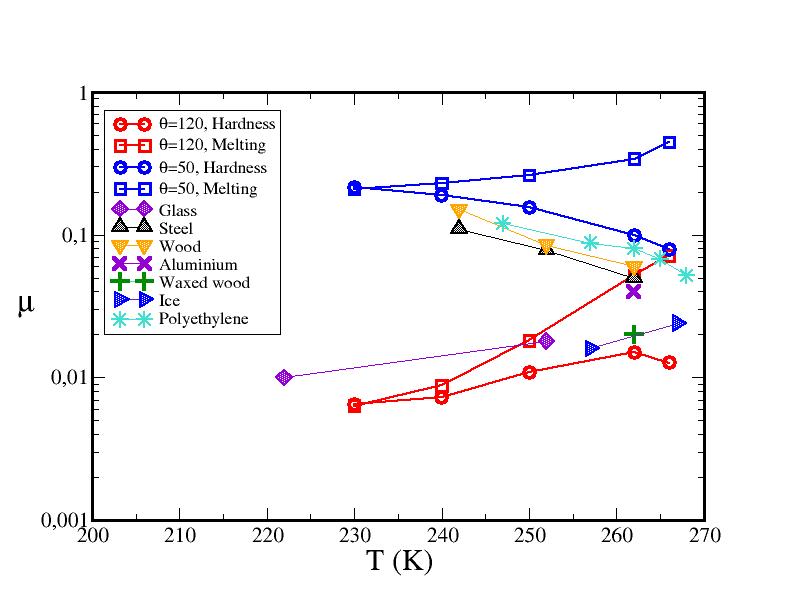
Figure 9: Consistency with experimental friction coefficients. Figure displays estimated friction coefficients at $U=5$ m/s from this work (empty symbols) with experimental data for different materials and sliding speed between 0.05 and 8 m/s (filled symbols). Empty squares correspond to friction coefficients estimated from the indentation hardness as reported in Liefferink et al. (13). Empty circles are obtained from the melting pressure. Experimental results are: Liefferink et al.(13), glass sphere on ice, $U\approx 0.05$ m/s (violet diamonds); Budnevich and Derjaguin (10),steel on ice, $U\approx 0.3$ m/s (grey triangles); Budnevich and Derjaguin (10), wood on ice, $U\approx 0.3$ m/s (orange triangles); Bowden (9), aluminium on ice, $U=5$ m/s (violet X); Bowden (9),waxed wood on ice, $U=5$ m/s (green cross). Oksanen and Keinonen (22),ice on ice (blue triangles), $U=3$ m/s; Stamboulides et al. (SI Appendix Ref.[15]) Ultra High Molecular Weight Polyethylene on ice at $U=2$ m/s (turquoise starts).

Figure 9 displays the friction coefficients estimated from $\mu=\tau/p_{i}$, with $p_{i}$ either equal to the indentation hardness, $p_{H}$ or the melting pressure, $p_{m}$, for hydrophobic and hydrophilic sliders. The results displayed, bracket experimental measurements of friction coefficients at similar sliding speeds, and show either increasing or decreasing friction coefficients with T, which are the two possible outcomes encountered in experiments depending on the material, as shown in the figure.

Shear Thinning

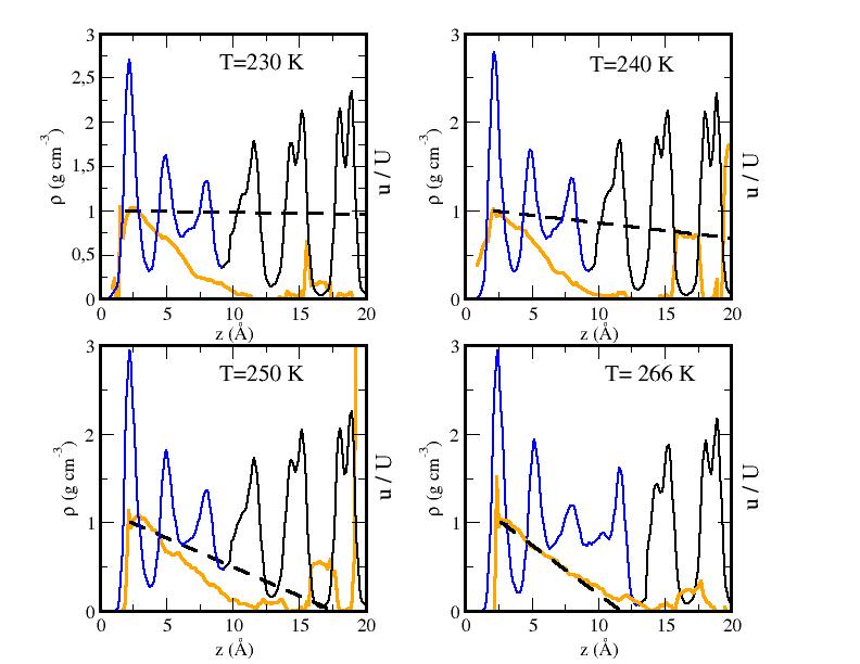
Figure 7: Structure and velocity flow of the premelted film during sliding. Results are shown for a sliding experiment on the hydrophilic wall ($\theta=50^{\circ}$) at $p=1$ atm, and $U=5$ m$/$s during 10 ns. The density profile in g cm^-3 (left axis) is shown as a continuous line, with blue colour for the region where liquid-like water is the majority phase and black colour where ice is the majority phase. Since these systems exhibit substantial frictional melting for temperatures below 262 K, the density profiles now correspond to the average obtained during the full 10 ns (c.f. Fig.4) for the equilibrim density profiles of the same system). The thick orange lines display the velocity profile in units of the sliding velocity (right axis). The dashed black line is the hydrodynamic flow profile predicted from the model of Eq. (1) in the main text. Note complete failure of the model at the two lowest temperatures due to substantial shear thinning. Panels correspond to different temperatures as indicated.

Using the model of Eq.(1) in the main text, which assumes bulk Newtonian viscosity, the prediction of the hydrodynamic film thickness that is obtained, $d_{H}=\eta u_{s}/\tau$, is orders of magnitude too large at 230 and 240 K, and about two times larger at 250 K. This results in predicted flow profiles that have an extremely low decay, as shown in Figure 7. Clearly, the correct shear stress can only be predicted from Eq.(1) of the main text if we assume a much smaller effective viscosity.

As noted in the main text, shear rate dependent viscosities can occur at low temperature for shear rates larger than a temperature dependent threshold value, a phenomenon known as shear thinnig, c.f. Ref.(2) and SI Appendix Ref.[3, 5]. Recently, de Almeida Ribeiro and de Koning studied the rheology of supercooled water with the TIP4P/Ice model and found significant shear thinning below 250 K for shear rates above $10^{9}$s^-1, which is roughly the shear rate attained in our simulations, c.f. Ref.(50). Therefore, we expect the small effective viscosities required to describe the actual shear stress in the system to result from shear thinning.

According to the Eyring theory of shear thinning (SI Appendix Ref.[5]), the shear viscosity of a fluid obeys the following equation:

$$\frac{\eta(\dot{\gamma})}{\eta(0)}=\frac{\tau_{0}}{\dot{\gamma}\eta(0)}\sinh^{-1}\left(\frac{\dot{\gamma}\eta(0)}{\tau_{0}}\right)$$ (2)

where $\eta(0)$ stands here for the bulk Newtonian viscosity, and $\tau_{0}$ is a threshold shear stress above which shear thinning becomes significant. The shear threshold depends on the temperature as $\tau_{0}=\frac{k_{B}T}{v_{a}}$, where $k_{B}$ is Boltzmann’s constant and $v_{a}$ is an activation volume in the order of the molecular volume.

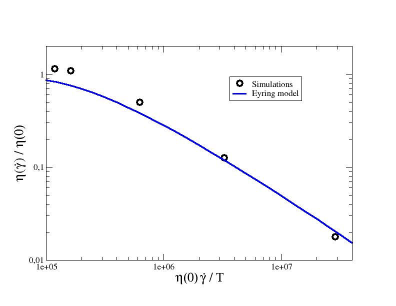
Figure 10: Shear thinning of premelting layers. The circles display the ratio of shear rate dependent viscosity to bulk Newtonian viscosity $\eta(\dot{\gamma})/\eta(0)$, as a function of the single variable $\eta(0)\dot{\gamma}/T$. The full lines are a fit to the Eyring model of shear thinning.

As shown in Fig. 10, this single parameter model describes in reasonable agreement the shear rate dependent hydrodynamic viscosities obtained from our simulations as $\eta(\dot{\gamma})=\tau d_{C}/u_{s}$. Moreover, the fit provides $v_{a}=1.5\cdot 10^{-28}$ m³, which corresponds to an effective radius $\sim 3\cdot 10^{-10}$ m of the same order of magnitude as the molecular radius, in agreement with expectation from the Eyring model.

Since $\sinh^{-1}(x)\approx\ln(x)$ for large $x$, the Eyring model predicts a shear stress $\tau=\tau_{0}\ln(\dot{\gamma}\eta(0)/\tau_{0})$ which, in view of $\dot{\gamma}\approx U/d_{C}$, yields a logarithmic dependence of shear stress with sliding velocity, as found in Ref.(13), but see also SI Appendix Ref.[3]. It follows that the friction coefficient, $\mu_{f}=\tau/p$, becomes of the order $\ln(U)/p$, as explained in the main text.

Contribution of Elasticity

For the hydrophobic slider at temperatures below 250 K, some amount of strain is observable in the simulation snapshots (c.f. Movie S3). Inspection of the molecular configurations shows a lateral displacement of about one lattice position in the direction of the slider. This corresponds to ca. $\frac{1}{4}b$, where $b$ is the crystal unit length in the sliding direction. This deformation is propagated over roughly 24 unit cells in the z-direction, of size $24c$ (with $b\approx 7.9$ Å  and $c\approx 7.4$ Å). This yields a small shear strain of $\gamma=\frac{1}{96}\frac{b}{c}\approx 0.01$. The shear modulus of ice in the temperature range studied is about $G=3$ MPa, according to Ref.(11). Therefore, the shear stress expected from the elastic deformation is $\tau=G\gamma=3\cdot 10^{-2}$ MPa, which is just a small fraction of the full shear stress measured in the simulations (c.f. Table 4). Interestingly, a small elastic response has also been measured in recent experiments by Canale et al.(14).

Methods

Model and setup

Water was modeled with the TIP4P/Ice force field, Ref. (33). Wall-water interactions were implemented with a force-shifted Lennard-Jones potential between wall atoms and water oxygens. For the wall-oxygen interactions, we chose $\sigma_{wo}$ equal to $\sigma_{oo}$ in the TIP4P/Ice model, and tuned the wall-oxygen $\epsilon_{wo}$ to $f\epsilon_{oo}$, with $f=\{1,2,3,4\}$. All dispersion interactions were truncated at 1 nm. An initial configuration of ice Ih oriented along the basal direction was prepared by replicating a pseudo-orthorombic unit cells of size $(2\times a)\times b\times c$, with 16 water molecules each. The bulk slab consisted of an arrangement of $4\times 4\times 15$ such cells, prepared so as to leave a half terminated bilayer exposed on the surface. Notice that in view of the limited amount of premelting observed, the simulation cells are unnecessarily large in the perpendicular direction, since the stress tensor components decay exponentially fast. A random hydrogen bond network with total zero dipole moment was created following Ref.(46). The wall consisted of a stack of three close–packed planes in a face-centered cubic (FCC) arrangement oriented along the (111) direction. A perfect match of the wall with the ice basal face is achieved by choosing a wall unit cell of size $a$, $b=\sqrt{3}a$ and $c=\sqrt{6}a$. For each temperature and pressure, we slightly rescaled the wall and ice unit cells to the corresponding equilibrated ice lattice. The ice slab was then sandwiched between the walls, and the whole system was placed in a simulation box under periodic boundary conditions, leaving a gap between the walls across the boundary conditions.

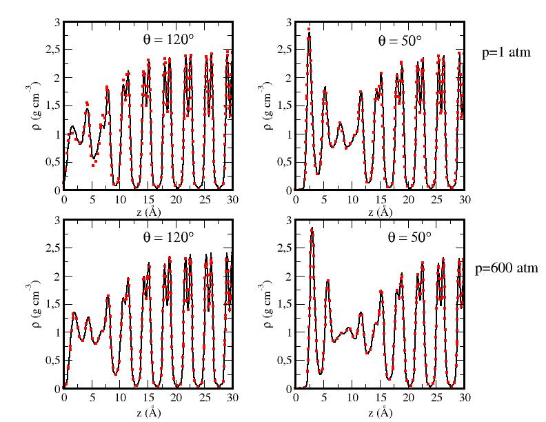
Figure 11: Influence of surface preparation on interfacial premelting. The full lines correspond to equilibrium density profiles obtained from an ice slab with a half terminated bilayer as the initial configuration. The symbols correspond to equilibrium density profiles obtained from simulations with an equilibrated ice/vapor interface as the initial configuration. Results are shown for $T=262$ K, with pressures of 1 and 600 atm and contact angles of $\theta=120^{\circ}$ and $50^{\circ}$ as indicated in the panels.

In order to save computational time, we do not put the walls in contact with a fully equilibrated ice/vapor interface at the relevant temperature. Instead, we have found that arranging the bulk ice lattice such that the external layer of the slab is a half terminated bilayer, instead of a full bilayer, does well the job. We illustrate this in Fig.11, which shows that the final equilibrated density profile is exactly the same, whether the simulation starts from the half terminated bilayer of a pre–equilibrated ice/vapor interface. Care must be taken when one puts directly the fully terminated bilayer in contact with the wall. In this case, the perfect wall match can stabilize an ice slab with no premelting layer whatsoever for a long time.

Analysis

The CHILL+ order parameter was employed to label water molecules in liquid-like and solid-like categories. Molecules labeled as bulk crystalline or interfacial crystalline (mainly Ih, Ic and interfacial Ih ice) were assigned as solid-like, and the remaining molecules were assigned as liquid-like. Parallel diffusion coefficients of the interfacial layer were calculated by monitoring the mean squared displacement of liquid–like molecules within the assigned interfacial region. Bulk transport coefficients were calculated using equilibrium Molecular Dynamics in the NVT ensemble. Diffusion coefficients were evaluated from mean square displacements and shear viscosity from Green-Kubo relations. Velocity profiles were smoothed using an unweighted moving average with spatial extent of 4 Å.

Implementation of the CHILL+ order parameter

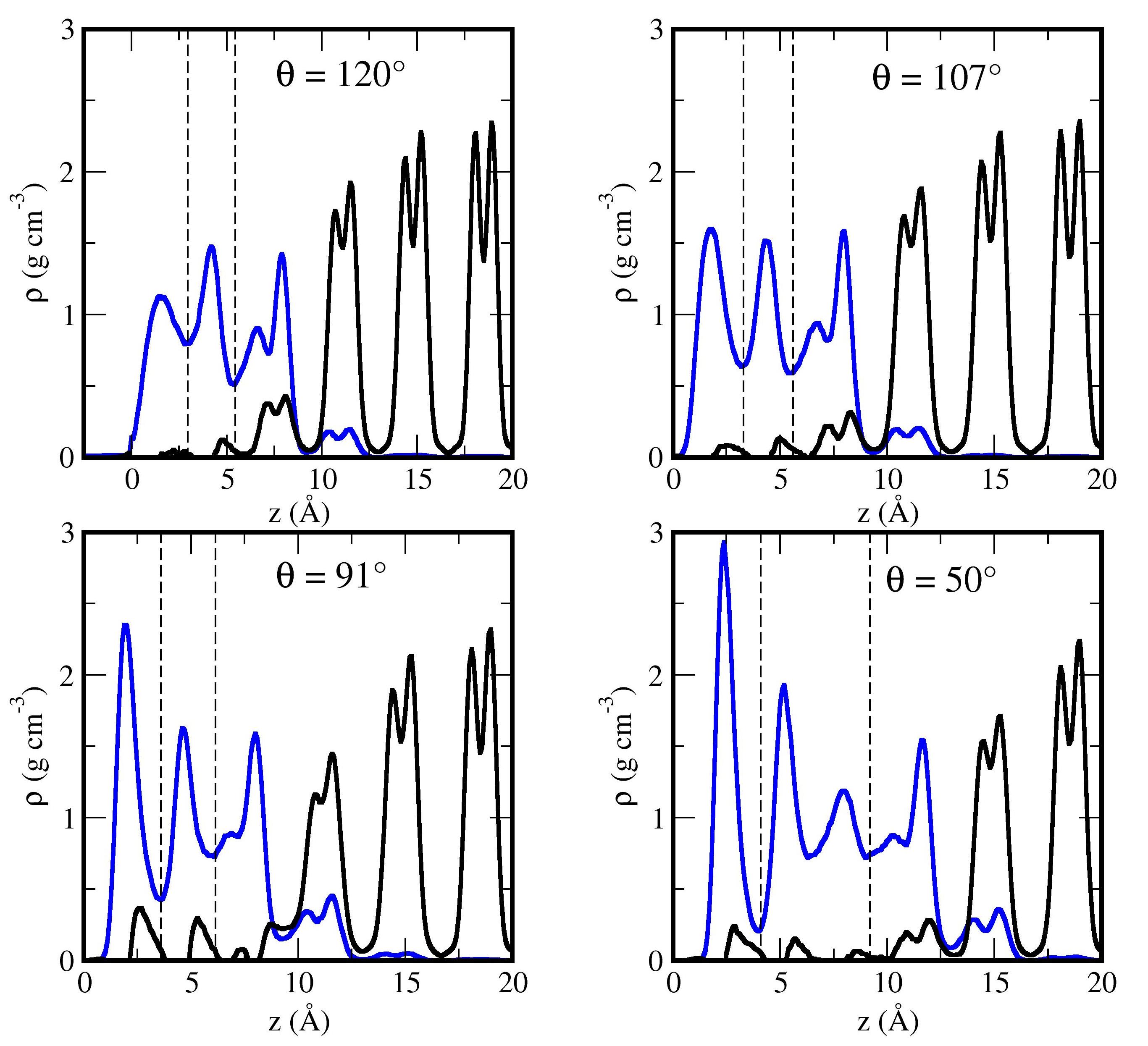
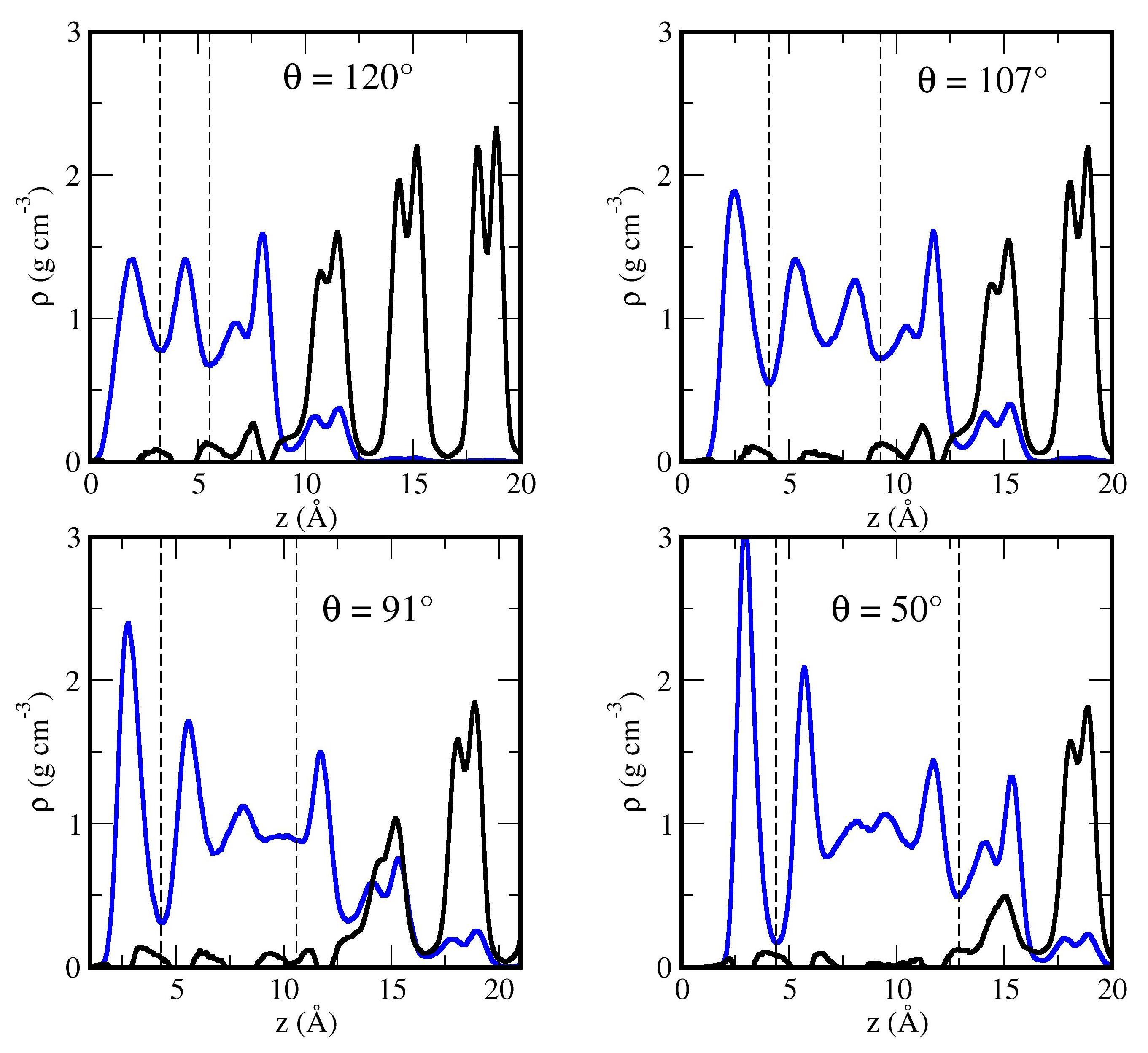
Figure 12: Structure of the interfacial premelting films at $p=1$ atm (left) and $p=600$ atm (right). The solid blue lines are the densities of liquid-like molecules, and the black lines correspond to densities of solid-like molecules. Notice a small penetration of solid-like molecules into the interfacial premelting film. Films at $p=600$ atm are significantly thicker than those found at $p=1$ atm.

In order to characterize the premelting film, each water molecule in the system is labeled according to the CHILL+ algorithm, Ref.(37). This algorithm allows one to identify ice allotropes as well as clathrates and interfacial ice Ih. To determine the amount of liquid-like and solid-like molecules we proceed as follows. First, we have identified the largest ice cluster and labeled all the molecules as solid-like molecules. In our case, this lumped regular ice Ih, interfacial ice Ih, and ice Ic into the solid-like category. We have found that CHILL+ treats some of the water molecules as mislabeled due to not fulfilling any of the criteria specified in Ref.(37).To assign them in either the solid or liquid group, we visualized the system and found that they always appeared within the liquid layer. Therefore, they are also included in the group of liquid-like molecules. Figure 12 displays results for the density of solid and liquid-like molecules. The plot shows that solid-like molecules penetrate slightly within the premelting layer, with some small oscillatory behavior found at high pressure. The presence of small ice patches could result in an additional viscoelastic response that is not taken into account in our model of Couette flow with slip. The consistency of the model indicates that viscoelastic contributions must be small in the regime studied in this work.

Measure of shear stress and test of barostat

The ice sample was compressed by imposing a force $F_{z}=\pm PA/N_{w}$ perpendicular to the interface in the direction of bulk ice on each of the wall atoms, c.f. Ref.(29,30,38) and SI Appendix Ref.[6, 7, 8].

The pressure exerted by the wall on the fluid must be balanced by the corresponding force exerted by the fluid on the wall. Whence, it must follow (c.f. SI Appendix Ref.[9]):

$$p_{z}=-\frac{1}{A}\int\frac{d\phi}{dz}\rho({\bf r})d{\bf r}$$ (3)

where $\phi$ is the potential energy between wall atoms and water molecules and $\rho({\bf r})$ is the density profile. For an atomically resolved density field, this amounts to the calculation of:

$$p_{z}=\frac{1}{A}\sum_{i}f_{z}({\bf r}_{i})$$ (4)

where $f_{z}$ is the $z$ component of the force exerted by the wall on a water molecule at ${\bf r}_{i}$, and the sum runs over all water molecules within the cutoff distance from the wall. We use this result as a test of consistency for the barostat and find excellent performance as illustrated in Table  3 and Table  4.

Likewise, the shear stress $\tau$ is calculated from the total force exerted by the wall atoms on the water molecules in the direction of the slider. Whence, $\tau=p_{x}$, and

$$p_{x}=\frac{1}{A}\sum_{i}f_{x}({\bf r}_{i})$$ (5)

with the sum convention as explained in the previous equation.

Estimation of contact angles

The wettability of the substrates is characterized by the contact angle of water sessile droplets at ambient temperature, T=298 K. Unfortunately, measuring contact angles is not a trivial matter, because they exhibit a very large system size dependence due to line tension effects (SI Appendix Ref.[10, 11]). In order to estimate the macroscopic contact angle, $\theta_{\infty}$, we calculated equilibrium contact angles for small droplets with 2304 and 5120 water molecules, and extrapolated to the infinite droplet size as (SI Appendix Ref.[12]):

$$\cos(\theta)=\cos(\theta_{\infty})-\frac{\tau}{\gamma_{lv}}\times\left(\frac{1}{R\sin(\theta)}\right)$$ (6)

where $\tau$ is the line tension and $\gamma_{lv}$ is the liquid-vapor surface tension.

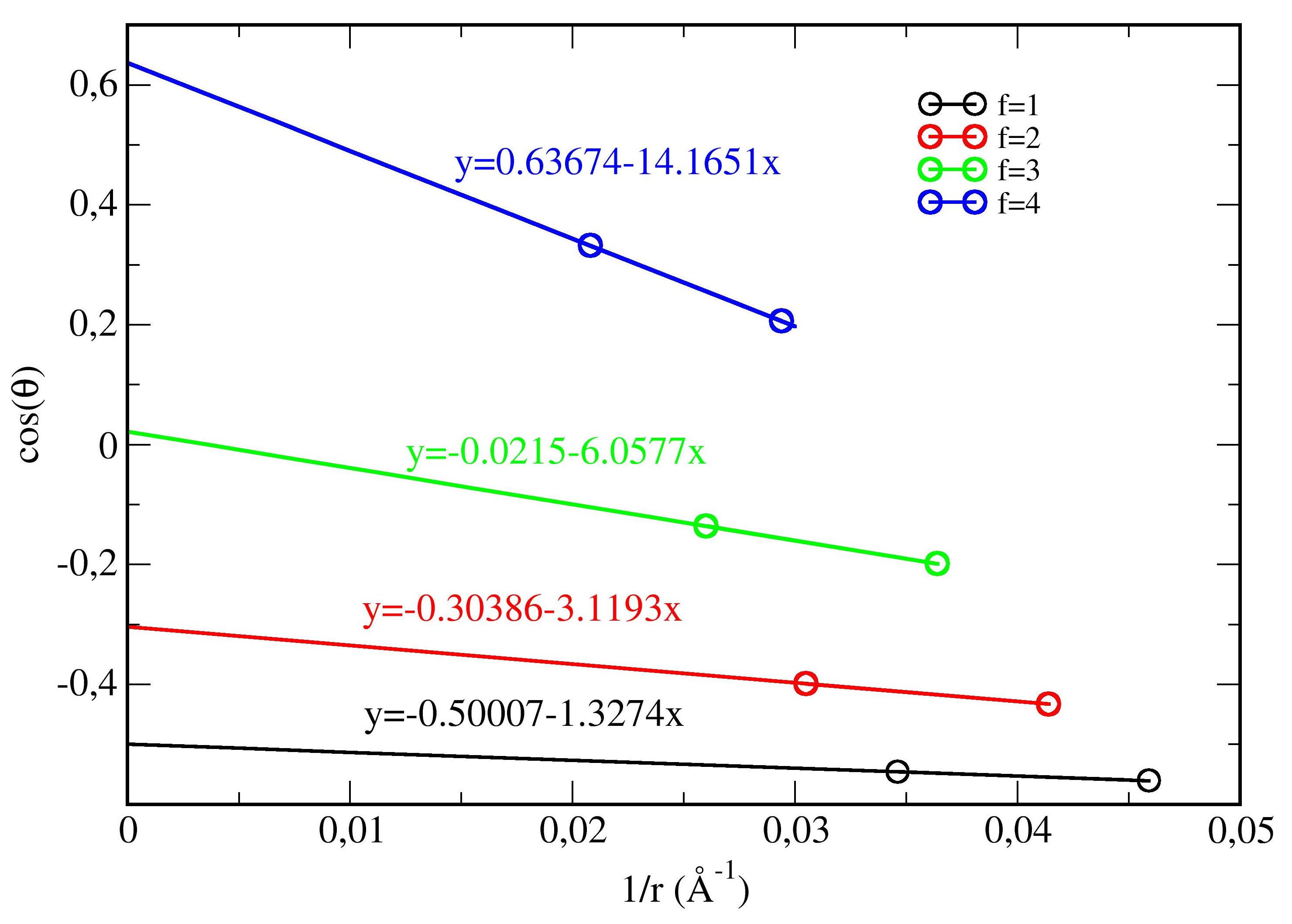
Figure 15: Measuring macroscopic contact angles. The finite size contact angles are extrapolated to infinite size in a plot of $\cos(\theta)$ vs $1/r$ where $r=R\sin(\theta)$.

Based on the values of the contact angles extracted from these simulations (cf. Table 5) we have extrapolated the curves shown in Figure 15 to $1/r=0$ where $r=R\sin(\theta)$. In this notation, the $R$ and $r$ refers to the radius of an auxiliary sphere and the radius of the base of the drop, respectively. Estimated values of the contact angles in the infinite droplet size are:

f=1 $\theta_{\infty}=120^{\circ}$

f=2 $\theta_{\infty}=107^{\circ}$

f=3 $\theta_{\infty}=91^{\circ}$

f=4 $\theta_{\infty}=50^{\circ}$

To measure the equilibrium contact angles of small spherical droplets we first simulated samples of a bulk liquid water in the $NpT$ ensemble for 15 ns at $T=298$ K and $p=1$ atm. Then, the water parcel was placed on the solid surface and allowed to equilibrate. The relaxation of the initial configuration is very slow. Simulations were carried out over 60 to 100 ns at $T=298$ K in $NVT$ ensemble in order to attain meaningful averages. From the trajectories collected over the final 10 ns of the simulations average density profiles $\rho(x,y)$ have been evaluated following the procedure described elsewhere (SI Appendix Ref.[13]). Briefly, the droplet has been divided into cylindrical slabs of the same width and within each, rectangular prisms have been further defined in which the average density has been calculated. The interfacial points of each slab have been located as $\rho(x,y)=(\rho_{liquid}-\rho_{vapor})/2$. The resulting density profile is fitted to a spherical cap of radius $R$, centered at position $z_{0}$ (SI Appendix Ref.[13]). In order to calculate the values of the contact angles, the curves have been extrapolated to the bottom of the droplet. Estimated error in the contact angle value is $\pm 2^{\circ}$ depending on the fitting, i.e. whether we fit entire drop or up to the $3/4$ of its height.

Similarly to all previous simulations, the charge structure factors were evaluated with a grid spacing of $1$ Å and the fourth order interpolation scheme. It resulted in the $54\times 48\times 30$ ($72\times 64\times 40$) vectors in the $x,y,z$ reciprocal directions, respectively, for 2304 (5120) water molecules. In the case of the simulations for droplets sitting on a solid surfaces, the number of vectors were equal to $150\times 144\times 100$ ($200\times 180\times 120$) in the $x,y,z$ reciprocal directions, respectively, for 2304 (5120) water molecules.

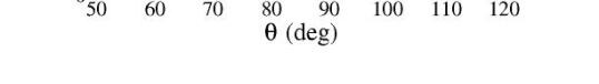
Figure 5: Quasi-Bulk like diffusivity of the premelting film. Results are shown for $T=262$ K and $p=1$ atm (left) and $p=600$ atm (right). The thick dashed line stands for the bulk diffusion coefficient. The remaining lines correspond to parallel diffusion coefficients of liquid-like molecules in different regions of the premelting film: Adsorption layer next to the wall (green squares); Adsorption layer next to ice (red diamonds); and quasi-bulk central region (blue circles).

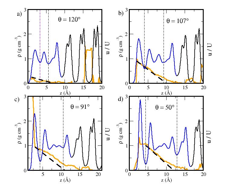
Figure 6: Structure and velocity flow of the premelted film during sliding. Results are shown for a sliding experiment at $p=600$ atm, $T=262$ K and $U=5$ m$/$s during 10 ns. The equilibrium density profile in g cm^-3 (left axis) is shown as a continuous line, with blue colour for the region where liquid-like water is the majority phase and black colour where ice is the majority phase. The premelting film is divided into two adsorption layers next to the wall and bulk ice and a central quasi-bulk region, as illustrated by vertical dashed lines. The thick continuous lines display the velocity profile in units of the sliding velocity (right axis). The dashed black line is the hydrodynamic flow profile predicted from the model of Eq. (1) in the main text. Notice a smaller extent of slip compared to results at $p=1$ atm. Panels correspond to different wall interactions (a) Hydrophobic wall, with $\theta=120^{\circ}$ (b) $\theta=107^{\circ}$ (c) $\theta=91^{\circ}$ (d) Hydrophilic wall with $\theta=50^{\circ}$.

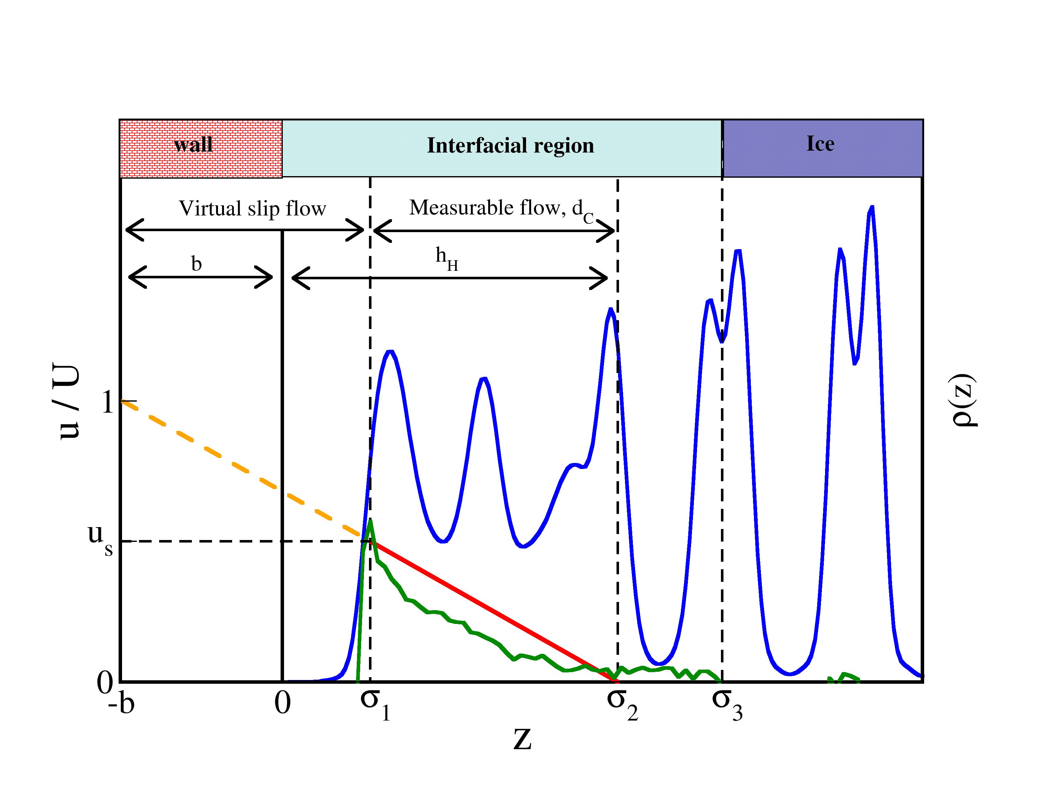
Figure 8: Sketch of hydrodynamic reference frame and boundary conditions. The blue lines display a sample density profile. The green line is a sample flow profile (average velocity in the direction of sliding as a function of perpendicular distance to the wall). The red line describes a hypothetical Couette flow profile required to describe the actual shear force from $\tau=\eta dU/dz$. In order to describe the actual flow in terms of a model of Couette flow with slip, $\tau=\eta U/(b_{w}+h_{H})$, we place the origin of the hydrodynamic reference frame $z=0$ at the first layer of rigid wall atoms. The flow profile attains its maximum value, $u_{s}$, at position $\sigma_{1}$, (close to the loci of the first adsorption peak of premelted water on the wall) whereupon, it shows a sharp drop and then vanishes. $\sigma_{2}$ is defined as a visual extrapolation of a straight line towards the bulk ice (close to the first adsorption peak of premelted water on bulk ice). A small tail of the flow profile persists up to the first ice bilayer, and vanishes at position $\sigma_{3}$. The difference between $\sigma_{2}$ and $\sigma_{3}$ corresponds to a small negative slip for the flow of water on ice. The extrapolated flow profile within the bulk substrate attains the velocity of the slider at a virtual position $z=-b$ which defines the wall slip length in our hydrodynamic model.

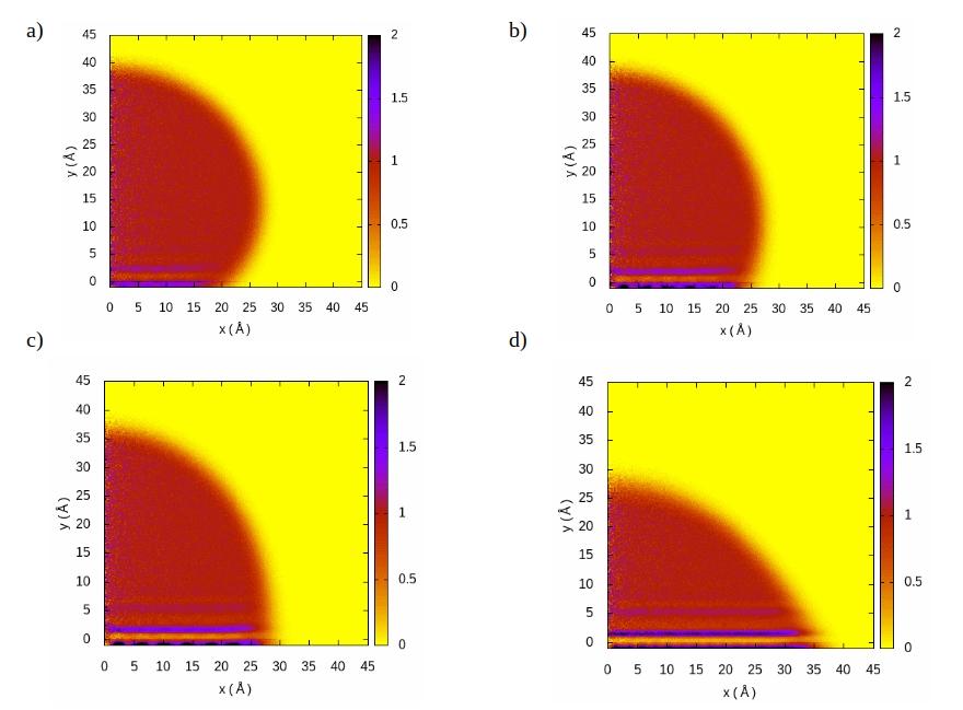
Figure 13: Density profiles $\rho(x,y)$ for sessile drops comprised of 2304 water molecules for interaction strength $f=1$ (a), $f=2$ (b), $f=3$ (c), and $f=4$ (d). Color bar depicts the density in the units of g cm^-3.

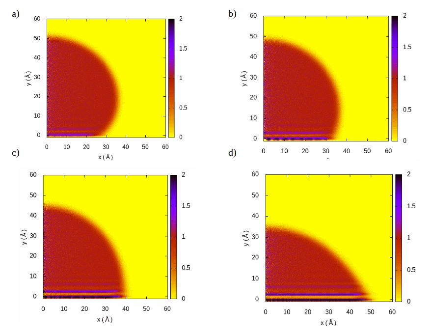
Figure 14: Density profiles $\rho(x,y)$ for sessile drops comprised of 5120 water molecules for interaction strength $f=1$ (a), $f=2$ (b), $f=3$ (c), and $f=4$ (d). Color bar depicts the density in the units of g cm^-3.

f	p (atm)	$D$ ($10^{-10}$m${}^{2}\cdot$s${}^{-1})$	$\eta$ (mPa$\cdot$s)	$z_{w}$ (Å)	$\sigma_{1}$ (Å)	$\sigma_{2}$ (Å)	$u_{s}/U$	$\tau$ (atm)
1	1	2.4	8.4	-1.89	0.96	7.6	0.1	70
2	1	2.4	8.4	-1.16	1.3	8.2	0.5	301
3	1	2.4	8.4	-0.65	2.	10	0.85	485
4	1	2.4	8.4	-0.16	2.6	12.5	1.	460
1	600	3.5	5.4	-1.35	1.1	10.1	0.25	118
2	600	3.5	5.4	-0.41	2.0	12.5	0.9	301
3	600	3.5	5.4	0.06	3.	15.3	0.95	305
4	600	3.5	5.4	0.31	4.5	15.4	1.	360

Table 1: Measure of hydrodynamic boundaries in the sliding experiments at $T=262$ K and various pressures. The simulation setup has the origin of coordinates close but not exactly at the wall position, which is allowed to move freely. $z_{w}$ is the average wall position; $\sigma_{1}$ and $\sigma_{2}$ are the hydrodynamic boundaries estimated from visual inspection of the velocity profiles and used to measure the Couette thickness, $d_{c}=\sigma_{2}-\sigma_{1}$. $u_{s}$ is the flow velocity at $\sigma_{1}$ in units of the slider velocity, $U$. The table also includes bulk diffusion coefficient and viscosity as obtained from equilibrium simulations.

f	T (K)	$D$ ($10^{-10}$m${}^{2}\cdot$s${}^{-1})$	$\eta$ (mPa$\cdot$s)	$z_{w}$ (Å)	$\sigma_{1}$ (Å)	$\sigma_{2}$ (Å)	$u_{s}/U$	$\tau$ (atm)
1	230	0.045	981	-2.33	-	-	-	36
4	230	0.045	981	-1.2	1.95	9.36	1.	1181
1	240	0.26	113	-2.52	-	-	-	38
4	240	0.26	113	-0.92	2.14	9.33	1.	994
1	250	0.95	24.0	-2.35	-	-	-	54
4	250	0.95	24.0	-0.55	2.31	10.01	1.	778
1	266	3.24	6.47	-1.86	1.9	8.9	0.11	58
4	266	3.24	6.47	-0.12	2.65	13.	1.	356

Table 2: Measure of hydrodynamic boundaries in the sliding experiments at various temperatures all at $p=1$ atm and various temperatures. The simulation setup has the origin of coordinates close but not exactly at the wall position, which is allowed to move freely. $z_{w}$ is the average wall position; $\sigma_{1}$ and $\sigma_{2}$ are the hydrodynamic boundaries estimated from visual inspection of the velocity profiles and used to measure the Couette thickness, $d_{c}=\sigma_{2}-\sigma_{1}$. $u_{s}$ is the flow velocity at $\sigma_{1}$ in units of the slider velocity, $U$. The table also includes bulk diffusion coefficient and viscosity as obtained from equilibrium simulations.

p (atm)	f (kcal mol-1)	$p_{z}\mathrm{equil}$ (atm)	$p_{z}\mathrm{shear,5m/s}$ (atm)	$p_{x}\mathrm{shear,5m/s}$ (atm)	$p_{x}\mathrm{shear,0.5m/s}$ (atm)
1	1.0	$18.9$	$3.4$	$70.4$
	2.0	$28.0$	$4.7$	$301$
	3.0	$26.0$	$9.6$	$485$
	4.0	$24.0$	$7.2$	$460$
200	1.0	$196$
	2.0	$208$
	3.0	$214$
	4.0	$194$
400	1.0	$389$
	2.0	$410$
	3.0	$410$
	4.0	$418$
600	1.0	$604$	$601$	$118$	$22.2$
	2.0	$592$	$605$	$302$	$39.7$
	3.0	$562$	$581$	$305$	$43.7$
	4.0	$610$	$595$	$360$	$43.0$
700	1.0	$705$
	2.0	$681$
	3.0	$671$
	4.0	$705$
800	1.0	$800$
	2.0	$797$
	3.0	$808$
	4.0	$827$

Table 3: Measure of stress components at the wall in equilibrium and shear simulations at $T=262$ K. The comparison of target pressure and perpendicular pressure measured at the wall serves to gauge the barostat. Results for the lateral force exterted by the wall on the water molecules allows to gauge the shear stress.

temperature (K)	f	$p_{z}\mathrm{equil}$ (atm)	$p_{z}\mathrm{shear,5m/s}$ (atm)	$p_{x}\mathrm{shear,5m/s}$ (atm)
230	1.0	6.83	3.61	36.0
	4.0	24.0	13.9	1181
240	1.0	5.93	4.35	38.5
	4.0	10.7	11.3	994
250	1.0	5.65	1.61	54.4
	4.0	17.1	8.70	778
266	1.0	9.50	3.04	58.6
	4.0	4.76	12.3	356

Table 4: Measure of stress components at the wall in equilibrium and shear simulations at $p=1$ atm. The comparison of target pressure and perpendicular pressure measured at the wall serves to gauge the barostat. Results for the lateral force exerted by the wall on the water molecules allows to gauge the shear stress.

No. of water mols.	f (kcal mol-1)	$\theta$ (deg)	$\cos(\theta)$	R (Å)	r (Å)	1/r (Å-1)
2304	1.0	124.16	-0.561	26.36	21.80	0.0459
	2.0	115.64	-0.433	26.8	24.15	0.0414
	3.0	101.47	-0.199	28.04	27.48	0.0364
	4.0	78.13	0.206	34.76	34.02	0.0294
5120	1.0	123.12	-0.546	34.56	28.94	0.0346
	2.0	113.5	-0.399	35.7	32.74	0.0305
	3.0	97.8	-0.136	38.75	38.39	0.0260
	4.0	70.6	0.332	50.9	48.01	0.0208

Table 5: The relation of contact angle values with respect to the interaction strength $f$ for two system sizes simulated.

Supplementary Movies

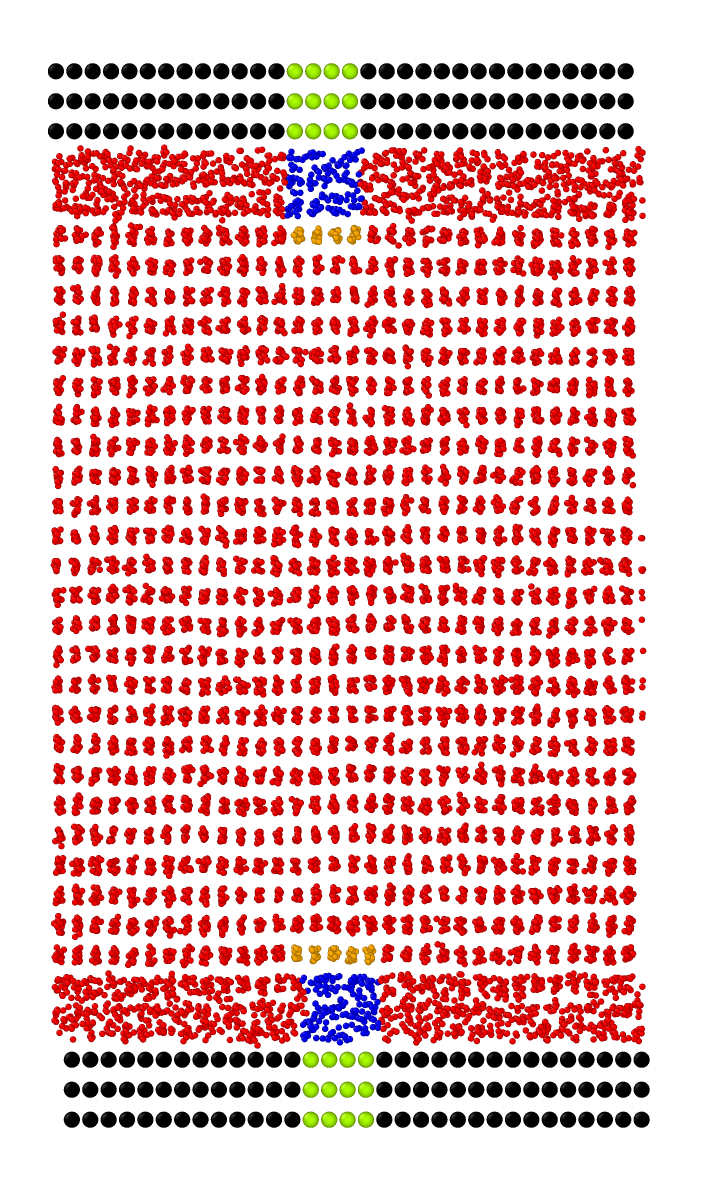
Figure 16: *

Movie S1: Sliding with slip at a hydrophobic wall. Movie displays the first 0.5 ns of a simulation at p=1 atm and T=262 K where a hydrophobic substrate with $\theta=120^{\circ}$ slides at a velocity of $U=5$ m/s. Notice how the wall slips past the premelting film, as illustrated by the blue tagged molecules.

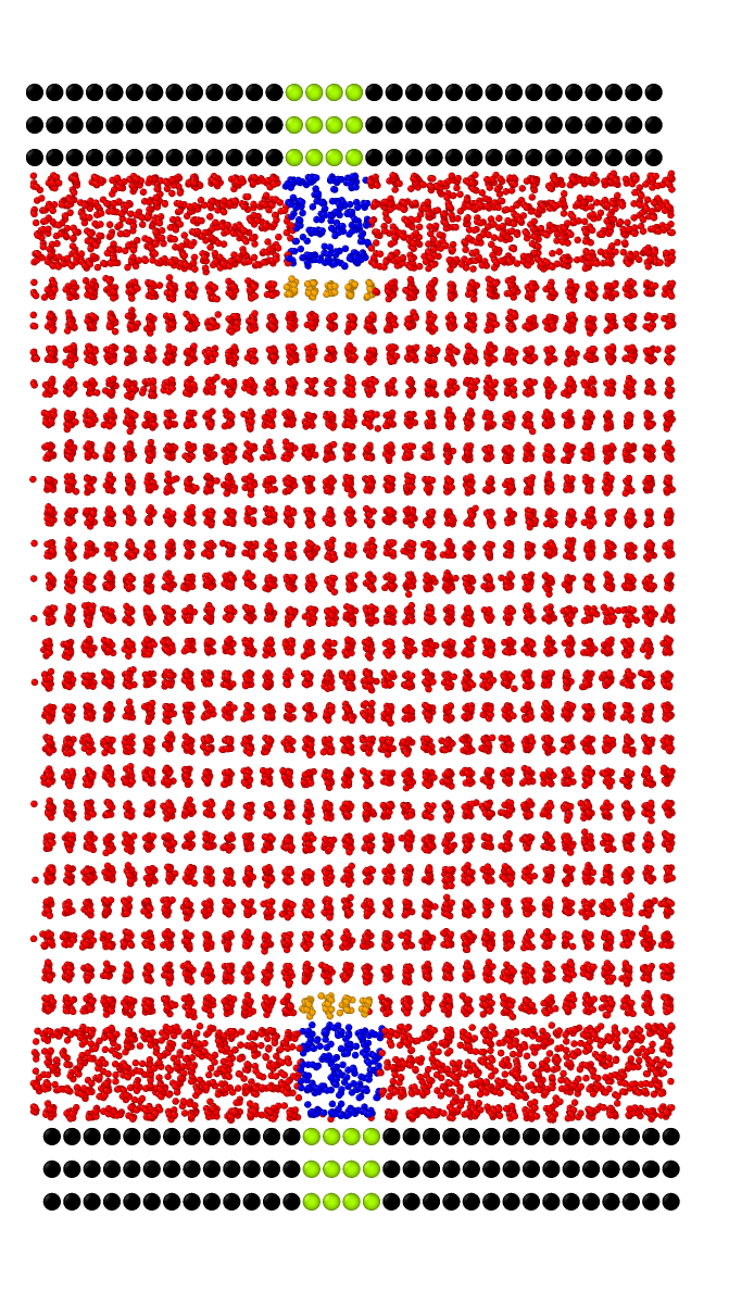
Figure 17: *

Movie S2: Sliding with stick at a hydrophobic wall. Movie displays the first 0.5 ns of a simulation at p=1 atm and T=262 K where a hydrophilic substrate with $\theta=50^{\circ}$ slides at velocity of $U=5$ m/s. Notice how the the wall-adsorbed layer sticks to the wall and moves at equal speed, as indicated by the blue tagged moelcules.

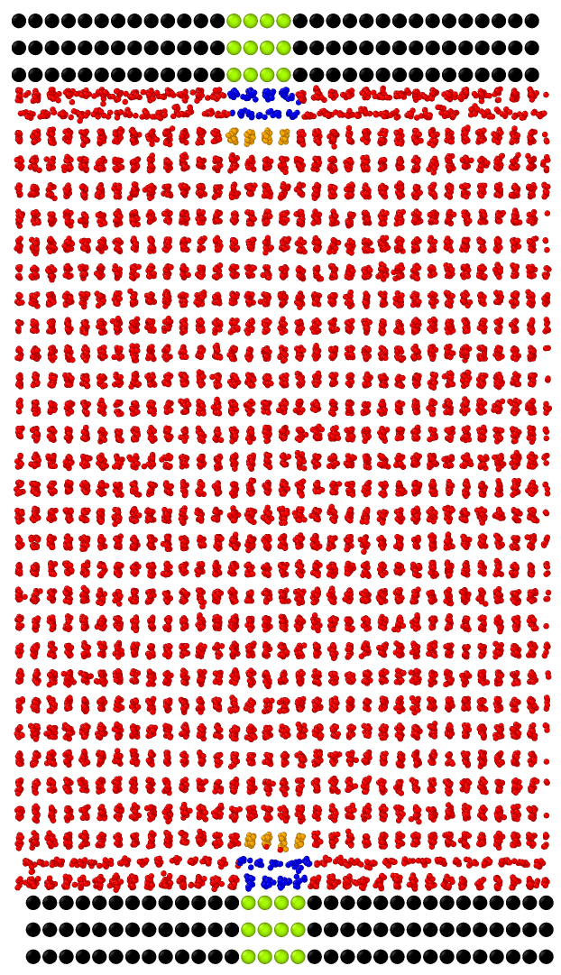
Figure 18: *

Movie S3: Frictional melting of ice. Movie displays the full 10 ns of a simulation at p=1 atm and T=230 K where a hydrophilic substrate with $\theta=50^{\circ}$ slides at velocity of $U=5$ m/s. Notice how the first ice bilayer melts already at 0.5 ns and an additional bilayer has melted after 5 ns.

References

- [1] Jorgensen WL, Madura JD, Swenson CJ (1984) Optimized intermolecular potential functions for liquid hydrocarbons. J. Am. Chem. Soc. 106:6638–6646.
- [2] Martin MG, Siepmann JI (1998) Transferable potentials for phase equilibria. 1. united-atom description of n-alkanes. J. Phys. Chem. B 102:2569–2577.
- [3] Müser MH, Urbakh M, Robbins MO (2003) Statistical mechanics of static and low-velocity kinetic friction. Adv. Chem. Phys. 126:188–272.
- [4] Santos-Flórez PA, Ruestes CJ, de Koning M (2020) Atomistic simulation of nanoindentation of ice ih. The Journal of Physical Chemistry C 124(17):9329–9336.
- [5] Spikes H, Jie Z (2014) History, origins and predictions of elastohydrodynamic friction. Tribol. Lett. 56:1–25.
- [6] Heyes DM, Smith ER, Dini D, Zaki TA (2011) The equivalence between volume averaging and method of planes definitions of the pressure tensor at a plane. J. Chem. Phys. 135(2):024512.
- [7] Marchio S, Meloni S, Giacomello A, Valeriani C, Casciola CM (2018) Pressure control in interfacial systems: Atomistic simulations of vapor nucleation. J. Chem. Phys. 148(6):064706.
- [8] Amabili M, et al. (2019) Pore morphology determines spontaneous liquid extrusion from nanopores. ACS Nano 13(2):1728–1738.
- [9] Henderson JR (1992) Statistical mechanical sum rules in Fundamentals of Inhomogenous Fluids, ed. Henderson D. (Marcel Dekker, New York), pp. 23–84.
- [10] MacDowell LG, Müller M, Binder K (2002) How do droplets on a surface depend on the system size? Colloids. Surf. A 206:277–291.
- [11] Vázquez U, Shinoda W, Moore P, Chiu CC, Nielsen S (2009) Calculating the surface tension between a flat solid and a liquid: a theoretical and computer simulation study of three topologically different methods. J. Math. Chem 45:161–174.
- [12] Pethica B (1977) The contact angle equilibrium. J. Colloid. Interface Sci. 62(3):567–569.
- [13] Włoch J, Terzyk AP, Gauden PA, Wesołowski R, Kowalczyk P (2016) Water nanodroplet on a graphene surface—a new old system. J. Phys.: Condens. Matter 28(49):495002.
- [14] Llombart P, Noya EG, Sibley DN, Archer AJ, MacDowell LG (2020) Rounded layering transitions on the surface of ice. Phys. Rev. Lett. 124(6):065702.
- [15] Stamboulides C, Englezos P, Hatzikiriakos SG (2012) The ice friction of polymeric substrates. Tribology Int. 55:59–67.