Measuring Equality and Hierarchical Mobility on Abstract Complex Networks

Abstract

The centrality of a node within a network, however it is measured, is a vital proxy for the importance or influence of that node, and the differences in node centrality generate hierarchies and inequalities. If the network is evolving in time, the influence of each node changes in time as well, and the corresponding hierarchies are modified accordingly. However, there is still a lack of systematic study into the ways in which the centrality of a node evolves when a graph changes. In this paper we introduce a taxonomy of metrics of equality and hierarchical mobility in networks that evolve in time. We propose an indicator of equality based on the classical Gini Coefficient from economics, and we quantify the hierarchical mobility of nodes, that is, how and to what extent the centrality of a node and its neighbourhood change over time. These measures are applied to a corpus of thirty time evolving network data sets from different domains. We show that the proposed taxonomy measures can discriminate between networks from different fields. We also investigate correlations between different taxonomy measures, and demonstrate that some of them have consistently strong correlations (or anti-correlations) across the entire corpus. The mobility and equality measures developed here constitute a useful toolbox for investigating the nature of network evolution, and also for discriminating between different artificial models hypothesised to explain that evolution.

1 Introduction

Hierarchies exist in every facet of our daily lives and understanding their ordering and dynamics is important to discern patterns and enable informed comparisons. A recent paper [15] studies how rankings evolve over time and the universal dynamics of hierarchies. In our work we apply a similar approach in the context of networks that evolve in time. The analysis of time evolving networks traditionally consists of tracking the evolution of network statistics such as degree distribution, clustering coefficient, assortativity and diameter. However, these overall statistics usually do not capture how individual nodes change their position within hierarchies, i.e., how their “status” improves or deteriorates over time.

In this paper we look at networks evolving in time, from the perspective of individual nodes, and we study how the characteristics of such nodes change as the network changes, with a special focus on degree centrality. A node’s degree could be considered as a measure of its status or importance e.g. the number of citations in a citation network [25] or friends in a social network. Obviously, not all nodes in a network have the same importance, and their roles can change over time as a result of the evolution of the network. Equality is a classical measure to quantify whether nodes tend to have the same centrality as other nodes, or whether centrality is concentrated in some nodes and not others. Similarly, hierarchical mobility measures whether nodes are frozen in their hierarchy position of high or low centrality. It is particularly interesting to consider how equality and hierarchical mobility evolve as a network changes.

Consider the Barabási–Albert (BA) model [1] and the Fortunato model [8] both of which produce power law degree distributions. In the Fortunato model a node attracts new nodes with a probability inversely proportional to the order of its arrival in the network. In BA that probability is proportional to the current degree of the node. Consider an instantiation of a BA model $G_{B}$ and a separate instantiation of a Fortunato model $G_{F}$. In both realisations, a node $s$ arriving earlier than a node $t$ has an advantage in gaining links. Imagine in both that $t$ by chance gains more nodes than $s$. In $G_{B}$ it is likely to continue to gain advantage over $s$ but in $G_{F}$ the node $s$ will retain its higher likelihood of gaining nodes. In $G_{B}$, therefore, this change of ranking where $t$ overtakes $s$, if it occurs, is more likely to be permanent.

Further to this we extend the focus to the importance of an individual node’s neighbourhood, and measure this by taking the mean degree of all nodes in said neighbourhood. The interaction between nodes can be somewhat measured by the impact a node has on its neighbourhood’s mean degree over time. Consider node $n$ which at $t_{1}$ is in a neighbourhood with a smaller than average mean degree and at $t_{2}$ is in a neighbourhood with a larger than average mean degree. Does this growth for the neighbourhood correlate with node $n$ itself having a large degree?

To look at equality we borrow the concept of the Gini coefficient [11] from classical economics which is generally used to measure wealth or income disparity. Traditional measures of economic or social mobility proved unsuitable for the setting of time evolving networks, hence we developed a taxonomy of six hierarchical mobility measures. These measures correlate the degree of individual nodes and their neighbourhoods between different points in time (see section 3).

To consider these measures on real network data we collected a corpus of 30 networks that evolve in time from a number of online sources. The code used to collect this data and analyse it for this paper is freely available under an open source licence.The networks are classified by their field and by structural properties.We used our equality measure and our taxonomy of mobility measures on this corpus to look for common patterns arising in different classes of networks. For example, we correlate the degree of a node at time $t_{1}$ with its change in neighbourhood mean degree between $[t_{1},t_{2}]$. We call this philanthropy as it can be thought of as measuring whether a large degree node helps its neighbours gain degree. Each network in our corpus can be classified by its equality, and the six measures in our mobility taxonomy. We used these seven dimensions to discriminate between different fields of study in complex networks.

We performed a principal component analysis and produced a “taxonomy landscape” plot within which types networks can be differentiated. Further, plotted each taxonomy aspect’s change over time for all of the networks in the corpus. Again, this produced plots which show many how the networks can be differentiated based on our taxonomy.

The measures introduced in this paper are a new tool for giving insight into how networks behave. For example, by looking at how network evolve in time over our seven dimension we can see which networks have ossified into a pattern of behaviour and which networks change how they evolve. Most networks in our corpus exhibit a mostly static degree hierarchy but, to our surprise, some exhibited a somewhat mobile degree hierarchy. There were large differences in equality between the networks in our corpus but the majority of networks we studied became more unequal over time.

2 Related Work

2.1 Individual Influence on Status Hierarchy Evolution

Abstract networks that evolve in time are an attempt to model the changes in real networks. The beginning of the pursuit for universal dynamics in the time evolution of such growing networks is often attributed to the famous Barabási-Albert (BA) [1] model. Their model replicates power-law degree distributions using simple evolution rules.

A more abstract approach was taken recently in [15] where the universal dynamics of ranking was explored for empirical systems. Through observing the dynamics of the ordered list, the authors built a framework consisting of only two key types; replacement and displacement. Either ranks are “swapped” at long ranges in the hierarchy, or ranks “diffuse” slowly between close by ranks. Their modelling approach consisted of calculating the probability of every individual to change rank to any other rank, and determined this to be monotonically increasing for “open” systems and symmetric for systems which are less open. Openness represents how fast new individuals to the system get into the top 100 ranks.

Approaches focusing on how networks evolve are becoming more numerous and many approaches try to replicate measured evolution dynamics. For instance, both [7] and [21] take the approach of measuring the effect node longevity has on its degree. It was found that a model which mimicked the preferential attachment of BA, but only for newly arrived nodes, did well in replicating the observed relationship between nodes and edges.

Another example is [34] which focused on mimicking the evolution of assortativity in social networks by calculating the probabilities of every node to be connected to $k$ neighbours at time $t$. From this they derived an analytical model for calculating the assortativity of a network throughout its lifetime, and found the model was a good fit with real social network data sets.

2.2 Equality

Determining the distribution of finite resources among many actors in a system is a useful metric for understanding whether such resources are being concentrated or spread out. In both sociology and economics this has been a popular area of interest with each concentrating on the distribution of “status” in societies. Economists use financial income as a quantifiable proxy for status, whereas sociologists tend to keep the definition more broad and qualitative.

A common measure of equality used by economists is the Gini coefficient [11] which is derived with reference to the Lorenz curve [19], a plot of wealth versus population. The Gini coefficient $G$ is given by

$$G=\frac{\sum^{n}_{i=1}\sum^{n}_{j=1}|x_{i}-x_{j}|}{2n^{2}\overline{x}}$$ (1)

where $x_{i}$ is the income of person $i$, $n$ is the number of people, and $\overline{x}$ is their mean income. This makes tracking changes in the equality measurements of populations a simple calculation. However, it does remove nuance from the result as it is a single number.

In sociology, one growing area of research has been network effects on inequality of status in social networks [12]. Much of the focus is aimed at how peer influence and network homophily [5] are large contributors to contagion of “practices” which improve a person’s status.

Our approach is to measure the Gini coefficient of the distribution of degree as it evolves over time.

2.3 Hierarchical Mobility

Tracking the mobility of status hierarchies over generations has also been a focus of Sociologists and Economists. Hierarchical mobility is the amount of movement individuals experience between hierarchy levels, and the hierarchies chosen depend on the focus of interest.

Sociological hierarchies focus on occupational classes [28] which are qualitative in nature and therefore have only a subjective [6] direction of hierarchy so do not apply to our purely network topology approach. An example mobility measurement is the “Log-Multiplicative Layer Effect Model” [2] which compares two matrices (called “layers” or “generations”) of class associations by assuming a uniform multiplicative association. This uniform association removes much of the much needed nuance between inter-generational class associations.

Economic hierarchies are built out of financial income bands [20] which are quantifiable and so readily ranked. A widely used mobility measurement used in economics is the Pearson correlation coefficient [26] $\beta=r(\ln{Y_{c}},\ln{Y_{p}})$ where $r(X,Y)$ is the Pearson correlation between numerical series $X$ and $Y$. This is usually used in conjunction with $\ln{Y_{c}}=\alpha+\beta_{p}\ln{Y_{p}}+\epsilon_{c}$ where $Y_{c}$ is the income of children, and $Y_{p}$ is the income of parents, $\alpha$ is a constant and $\epsilon_{c}$ is a fitted constant.

Our proxy for status in abstract networks is degree centrality which, like income bands, has a definite hierarchical direction. Instead of imposing arbitrary generations we study the evolution between two points in time $t_{1}$ and $t_{2}$. In section 3, we introduce more details of translating these hierarchical mobility measurements into our taxonomy of hierarchical mobility.

3 Measuring equality and hierarchical mobility in networks

3.1 Equality

Using equation 1 we can substitute in the degree of each node as $x_{i}$, the mean degree as $\overline{x}$ and the number of nodes as $n$. This is done at many time-steps throughout the life of a network and then the resulting coefficients are plotted against time to see how equality changes.

The income hierarchies used in economic analysis are very similar to degree in that they are numeric and a larger number is assumed to be a good proxy for status. However, the income of individuals fluctuate over their lifetime, both gaining and losing income. Our formulation of growing networks contain nodes that only ever increase their degree. This does not affect the calculation of equality, and moreover it allows for greater inference.

If a network is gaining a larger equality over time then the range of degree of nodes is getting narrower. As the networks are always growing it can be inferred in this case that high degree nodes are connecting to low degree more preferentially. Conversely, a lowering of equality over time suggests a divide in the connections being created. It can be inferred that lower degree nodes are more likely to attach to higher degree nodes, and less likely between themselves.

3.2 Mobility Taxonomy

As mentioned earlier, classical notions of social and economic mobility were not a good fit for the context of time evolving networks. To this end we introduced new measures that depend on the centrality of a node and how it evolves. In this work we consider only degree centrality.

To calculate the mobility of a node we consider the degree centrality of every node at time $t_{1}$ and the change of centrality in the period $[t_{1},t_{2}]$. If these are highly correlated it indicates that the nodes with highest centrality at $t_{1}$ gain the most in the period to $t_{2}$. We measure this correlation using the Pearson correlation coefficient and refer to this measure as mobility.

We also extended this to look at the mean centrality of each node’s neighbours at time $t_{1}$ and the mean gain of centrality for this same neighbour set in the period $[t_{1},t_{2}]$. This gives us four measures: node degree, change in node degree, mean neighbourhood degree and change in mean neighbourhood degree. Looking at the correlations between each of these gives us a taxonomy of six different mobility measures which are tabulated below.

Correlation	Change in degree	Mean neighbour degree	Change in mean neighbour degree
Degree	Mobility	Assortativity	Philanthropy
Change in degree		Community	Change in assortativity
Mean neighbour degree			Neighbour mobility

Table 1: The taxonomy of mobility related aspects

Correlating degree at time $t_{1}$ with the change in average neighbourhood degree to $t_{2}$ can be thought of as measuring how much a high status node helps its neighbours and we call this philanthropy. The correlation between neighbour mean degree at $t_{1}$ and the change in the period $[t_{1},t_{2}]$ can be thought of as neighbourhood mobility. The correlation between a neighbourhood’s mean degree at time $t_{1}$ and a node’s gain in degree between $[t_{1},t_{2}]$ could be considered as a measure of how much neighbourhood helps a node and we refer to it as community. The correlation between a node’s degree and its neighbours’ mean degree at $t_{1}$ is the well known assortativity. The correlation between a node’s change of degree and its neighbours’ mean degree between $[t_{1},t_{2}]$ can therefore be thought of as change in assortativity. These six measures together form a taxonomy for investigating how individual nodes and their neighbours interact and change over time.

4 Data set Corpus

To empirically measure the prevalence of each aspect of our taxonomy in many different types of network, we have collected 30 real networks. We have assigned each data set a type based on where the data has been collected, i.e social or transportation, and information about where to find them is available under an open source licence . Furthermore, we assigned each a category taken from the structural characteristics of the networks themselves, such as bipartite or the nature of newly joining nodes. For instance, citation networks grow by adding stars every iteration, i.e one node connected to all those it cites. The networks vary in size from 138 edges to nearly 1 million . All networks are treated as undirected and unweighted with added links never removed.

	Name	Description	Type	Structure	Nodes	Edges
a	College Messages [22]	Messages between students on a UC-Irvine message board	Social	Star	1,881	13,695
b	SCOTUS Majority [9]	Legal citations among majority opinions by SCOTUS	Citation	Star	33,442	199,374
c	Amazon Ratings [18]	Amazon user connects to all products they have rated	Economic	Bipartite	743,018	975,429
d	Apostles Bible [14]	Characters in the Holy Bible’s Acts of Apostles	Co-occurrence	Individual	75	160
e	Appollonius [14]	Characters in The Life of Apllonius of Tyana	Co-occurrence	Individual	92	138
f	Citations US Patents [13]	Citations among patents in the United States	Citation	Star	777,527	999,632
g	Classical Piano [24]	Transitions of chords in western classical piano music	Co-occurrence	Individual	141,571	501,033
h	Email EU [23]	E-mails between users at an EU research institution	Social	Star	986	16,006
i	Procurement EU [33]	Public EU procurement contracts	Economic	Bipartite	330,049	566,369
j	Facebook Wall [32]	Posts by users on other users’ Facebook wall	Social	Star	45,580	181,666
k	Lord Of the Rings [3]	Character co-occurrence in Lord of the Rings Trilogy	Co-occurrence	Individual	139	634
l	Luke Bible [14]	Characters in the Holy Bible’s Luke Gospel	Co-occurrence	Individual	76	203
n	PhD Exchange [29]	Exchange of PhD mathematicians between unis in the US	Citation	Star	230	3,643
o	Programming Languages [30]	Influence relationships among programming languages	Citation	Star	366	759
p	Reuters Terror News [4]	Word co-use in Reuters 9/11 coverage	Co-occurrence	Individual	13,265	146,985
q	Route Views [3]	Route Views internet topology	Computer	Individual	33,644	94,075
r	Reddit Hyperlinks Body [17]	Subreddit-to-subreddit hyperlinks from body of posts	Social	Clique	35,592	123,394
s	Reddit Hyperlinks Title [17]	Subreddit-to-subreddit hyperlinks from title of posts	Social	Individual	53,747	217,986
t	Hospital [31]	Contacts between everyone in a hospital ward	Contact	Spatial	75	1,132
u	Hypertext Conference [16]	Contacts among attendees of ACM Hypertext 2009	Contact	Spatial	113	2,192
v	Infectious [16]	Contacts during Infectious SocioPatterns 2011 event	Contact	Spatial	10,844	43,951
w	Office [10]	Contacts between individuals in an office building	Contact	Spatial	92	754
x	Primary School [27]	Contacts among students and teachers at a primary school	Contact	Spatial	242	8,298
y	AskUbuntu [23]	User answers or comments on questions on AskUbuntu	Social	Clique	157,709	502,966
z	MathOverflow [23]	User answers or comments on questions on MathOverflow	Social	Clique	24,506	198,040
A	StackOverflow [23]	User answers or comments on questions on StackOverflow	Social	Clique	38,379	618,519
B	SuperUser [23]	User answers or comments on questions on SuperUser	Social	Clique	124,528	541,466
C	UCLA AS [3]	UCLA AS level internet topology	Computer	Individual	38,055	224,545
D	US Air Traffic [23]	Flights among all commercial airports in the US	Transport	Individual	623	14,952
E	Wiki Talk [23]	Wikipedia users editing each other’s Talk page	Social	Individual	116,661	329,805

Table 2: Data sets used for network creation, limited to 1 million edges.

5 Results & Discussion

5.1 Equality

We plot the Gini Coefficient (GC) of all our corpus networks on the same axis and colour the data set based on the datatype shown in Table 2. The x-axis in figure 1 is normalised time where the maximum duration of each network has been normalised to be between [0,1], and 100 snapshots of equality have been calculated throughout the network’s lifetime. The y-axis shows the GC, where a higher value corresponds to a lower level of equality for the network.

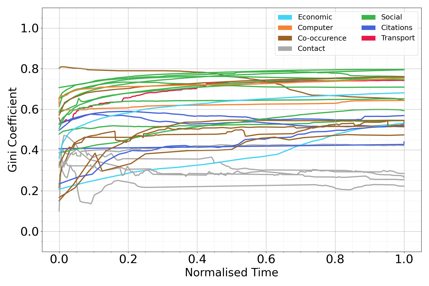
Figure 1: Equality of data set corpus networks coloured by data type over normalised time, where all network lifetimes are normalised to the range $0$ to $1$.

In Figure 1 the GC takes values over most of the possible range (0,1) with the values being contained between 0.2 and 0.8 from normalised time 0.2 onwards. Of the 30 data sets studied all but 4 rise in GC (becoming more unequal) between normalised time 0.0 and 1.0. he figure also shows some discrimination between the types of networks, for example social networks in general are most the unequal and contact networks most equal.

The contact networks are collected by measuring contact between people in physical space. Therefore the degree of a node is limited by the number of people that can be physically present in the space during the measurement interval. These limitations on network evolution would suggest a more equal distribution of degree as it is more likely that two individuals will spend time together than a less constrained system. Online social networks do not have this physical limitation. For example, if an individual is not interested in the software language Python, then they will not interact with the Python section of stackoverflow.com. This means there is less chance of densification as the interactions are less likely to occur than a physical contact network.

5.2 Mobility Taxonomy

To look at how the mobility taxonomy varies with time for every data set network we chose values of $t_{1}$ evenly spaced as the network grows. To achieve this we pick values of $t_{1}$ corresponding to $10,20,\ldots,90\%$ of the final number of edges being present and $t_{2}$ corresponding to all edges being present.

5.2.1 Taxonomy Aspect Evolution

These values of the mobility taxonomy were plotted against time to show how they individually evolve with time in figure 2. The data set types are again used to differentiate the networks, and it can be seen that most of the networks have a similar evolution for each of the aspects. However there are notable exceptions in each case.

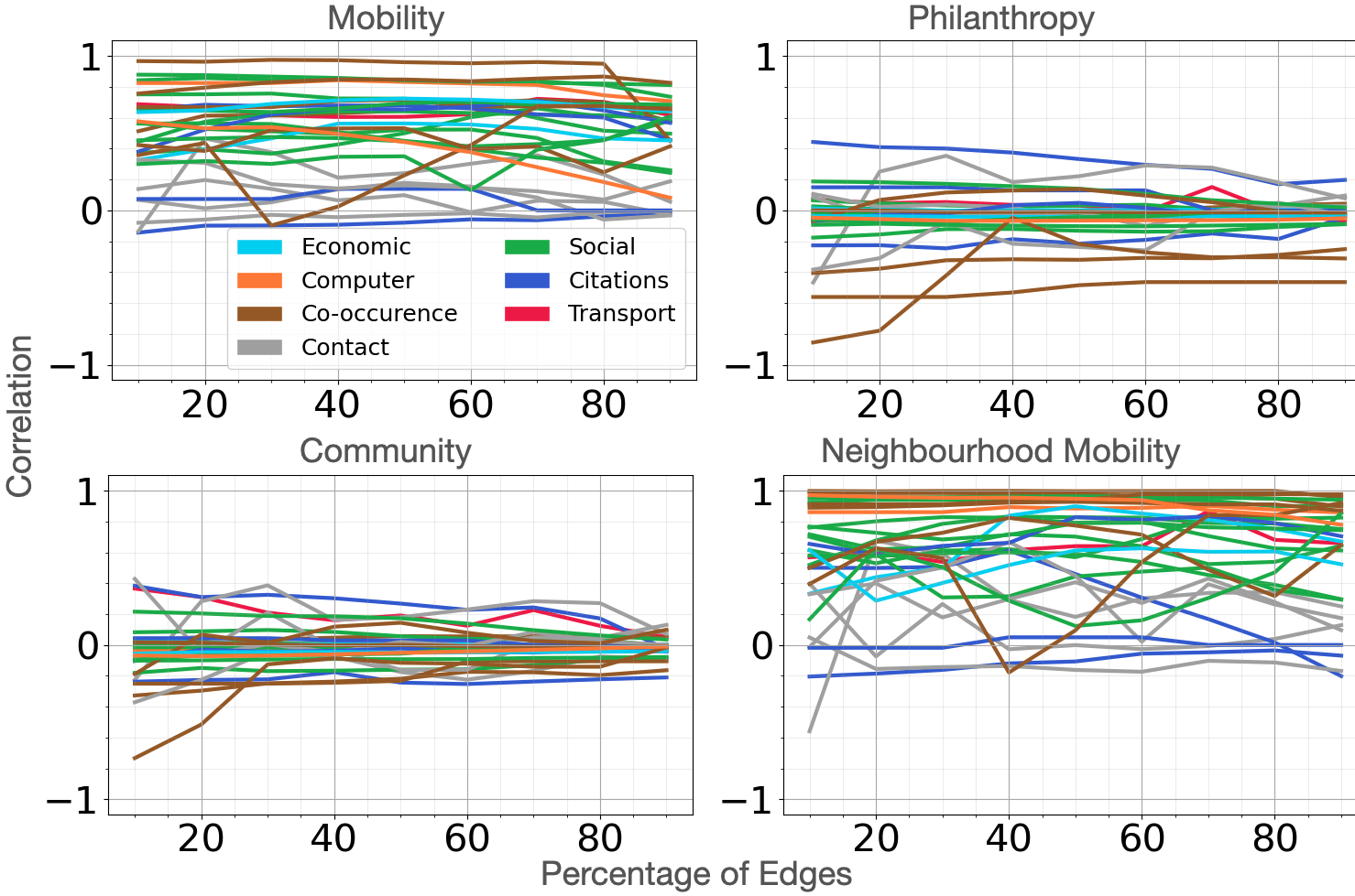
Figure 2: Every data set corpus network for each aspect of the mobility taxonomy coloured by data type. The x-axis represents $t_{1}$ characterised as percentage of life of the network. The y-axis shows the correlation coefficient as measured using Pearson correlation.

Mobility and neighbourhood mobility positively correlate with a coefficient of 0.79 at $10\%$ of edges, which can be seen in the vast majority of networks reaching high levels of correlation for both aspects. Positive correlation coefficients for these aspects signify a more static hierarchy of degree in the network over time (i.e individual nodes rarely change their place in the degree hierarchy). As static degree hierarchies are sometimes thought of as a given in real world network degree, it is unexpected we found limited evidence of networks which have a somewhat mobile degree hierarchy. However, this is largely in contact networks where, perhaps the large degree nodes happened to have many contacts at one time and getting the mobile degree hierarchy is merely regression to the mean.

The aspects community and philanthropy have a Pearson correlation of 0.48 at $10\%$ of edges. Some networks are positive or negative in both but most of the networks show very little either way. For those on the periphery, there is a noticeable trend towards zero for both positive and negative correlations suggesting a longer time in the network correlates with a more significant influence from these aspects. Negative values of philanthropy can be thought of as nodes that grow themselves but have a detrimental effect on the growth of their neighbours. This is largely seen in co-occurrence networks and we might think of a “prima-donna” effect where characters that gain attention drain attention from their co-stars.

5.2.2 Principal Component Analysis

To take the analysis further we correlated each aspect with each other, plus the Gini coefficient results at time $t_{1}$ for completeness, e.g all of the data set results for mobility with those of philanthropy. This resulted in a seven-dimensional matrix which we reduce to its two highest variance components using Principal Component Analysis for visualisation

Having time dependant values for the PCA means we are able to show how the networks evolve in time. These results are plotted in figure 3 with the data and structural types from Table 2 highlighted using colours and shapes. One striking feature is that many network are clustered together in the upper left quadrant of the graph. These networks are also much less prone to large changes in position, i.e they are more ossified, than those on the periphery of the cluster. A slight trend occurs in how the further the network is from the origin the more volatile its position on the PCA is over time. This volatility of position also correlates with a fewer number of nodes in the networks, i.e smaller networks have more changeability in their taxonomy aspects over time.

Figure 3: Principal component analysis of the mobility taxonomy, including equality, with each data set marked by its associated letter (see Table 2) on its first time-step. The plotted lines denote the data sets through 9 time-steps, each step plotted with a shape corresponding to its structure and the colour corresponding to its type.

6 Conclusions

In this paper we have shown how tracking the statistics of individual nodes and their neighbours, specifically the degree centrality, throughout the lifetime of the network can bring structural and developmental insight into the network’s evolution. Each of the mobility taxonomy aspects, along with equality, show different mechanisms underlying the evolution of a network and combining knowledge gained from each of them draws a vivid picture of how individual nodes interact with each other.

Also, running a PCA on the whole mobility taxonomy (plus equality) was shown to distinguish between networks into somewhat distinct categories. The time evolving PCA allowed for determination of network ossification and it was found that social networks are more likely to be ossified whereas co-occurrence and contact networks are less likely, though network size is also a contributing factor.

The techniques outlined in this paper are of great use for analysing trends of nodes in networks which evolve with time. Our main focus for future expansion is to delve deeply into the inter-node interaction dynamics of a single network and build understanding of causation for network-level phenomena from individual node interactions.

6.0.1 Acknowledgements

The authors wish to acknowledge the support of Moogsoft Ltd. for funding this research.

References

- [1] Barabási, A.L., Albert, R.: Emergence of scaling in random networks. Science 286(5439), 509–512 (10 1999). https://doi.org/10.1126/science.286.5439.509
- [2] Breen, R.: Social mobility in Europe. OUP Oxford (2004)
- [3] Clegg, R.G., et al.: Measuring the likelihood of models for network evolution. In: Proc. INFOCOM’09. pp. 272–277 (2009)
- [4] Corman, S.R., Kuhn, T., Mcphee, R.D.: Studying complex discursive systems. Human Communication Research (2002). https://doi.org/10.1111/j.1468-2958.2002.tb00802.x
- [5] Dimaggio, P., Garip, F.: Network effects and social inequality. Annual Review of Sociology 38, 93–118 (2012). https://doi.org/10.1146/annurev.soc.012809.102545
- [6] Erikson, R., Goldthorpe, J.H.: The constant flux: A study of class mobility in industrial societies. Oxford University Press (1992)
- [7] Fire, M., Guestrin, C.: The rise and fall of network stars. Information Processing and Management 57(2) (2020). https://doi.org/10.1016/j.ipm.2019.05.002
- [8] Fortunato, S., et al: Scale-free network growth by ranking. Physical Review Letters 96(21), 1–4 (2006). https://doi.org/10.1103/PhysRevLett.96.218701
- [9] Fowler, J.H., et al: Network analysis and the law. Political Analysis 15(3), 324–346 (2007). https://doi.org/10.1093/pan/mpm011
- [10] Génois, M., et al: Data on face-to-face contacts in an office building suggest a low-cost vaccination strategy based on community linkers. Network Science 3(3), 326–347 (2015). https://doi.org/10.1017/nws.2015.10
- [11] Gini, C.: Variabilità e mutabilità. Memorie di metodologica statistica (1912)
- [12] Granovetter, M.S.: The strength of weak ties. American journal of sociology 78(6), 1360–1380 (1973)
- [13] Hall, B.H., et al: The NBER patent citation data file: Lessons, insights and methodological tools. NBER Cambridge, Mass. (2001). https://doi.org/10.3386/w8498
- [14] Holanda, A.J., et al: Character networks and book genre classification. IJMPC 30(8) (2019). https://doi.org/10.1142/S012918311950058X
- [15] Iñiguez, G., Pineda, C., Gershenson, C., Barabási, A.L.: Universal dynamics of ranking. Nat Commun (2021), http://arxiv.org/abs/2104.13439
- [16] Isella, L., et al: What’s in a crowd? analysis of face-to-face behavioral networks. JTB 271(1), 166–180 (2011). https://doi.org/10.1016/j.jtbi.2010.11.033
- [17] Kumar, S., et al: Community interaction and conflict on the web. WWW pp. 933–943 (2018). https://doi.org/10.1145/3178876.3186141
- [18] Lim, E.P., et al.: Detecting product review spammers using rating behaviors. In: Proceedings of the 19th ACM international conference on Information and knowledge management. pp. 939–948 (2010)
- [19] Lorenz, M.O.: Methods of measuring the concentration of wealth. Publications of the American statistical association 9(70), 209–219 (1905)
- [20] Mayer, S.E., Lopoo, L.M.: Has the intergenerational transmission of economic status changed? JHR 40(1), 169–185 (2005). https://doi.org/10.3368/jhr.xl.1.169
- [21] Nsour, F., Sayama, H.: Hot-get-richer network growth model. In: International Conference on Complex Networks and Their Applications. pp. 532–543. Springer (2020)
- [22] Panzarasa, P., et al.: Patterns and dynamics of users’ behavior and interaction: Network analysis of an online community. Journal of the American Society for Information Science and Technology 60(5), 911–932 (2009)
- [23] Paranjape, A., et al: Motifs in temporal networks. WSDM, Proc. pp. 601–610 (2017). https://doi.org/10.1145/3018661.3018731
- [24] Park, D., et al: Novelty and influence of creative works, and quantifying patterns of advances based on probabilistic references networks. EPJ Data Science 9(1) (2020). https://doi.org/10.1140/epjds/s13688-019-0214-8
- [25] Redner, S.: Citation statistics from 110 years of physical review. Physics Today 58(6), 49–54 (2005). https://doi.org/10.1063/1.1996475
- [26] Solon, G.: Intergenerational income mobility in the united states. The American Economic Review pp. 393–408 (1992)
- [27] Stehlé, J., et al: High-resolution measurements of face-to-face contact patterns in a primary school. PLoS One 6(8) (2011). https://doi.org/10.1371/journal.pone.0023176
- [28] Szreter, S.R.S.: The genesis of the registrar-general’s social classification of occupations. The British Journal of Sociology 35(4), 522–546 (1984)
- [29] Taylor, D., et al: Eigenvector-based centrality measures for temporal networks. MMS 15(1), 537–574 (2017). https://doi.org/10.1137/16M1066142
- [30] Valverde, S., Sole, R.V.: Punctuated equilibrium in the large-scale evolution of programming languages. JRSI 12(107) (2015). https://doi.org/10.1098/rsif.2015.0249
- [31] Vanhems, P., et al: Estimating potential infection transmission routes in hospital wards using wearable proximity sensors. PloS One 8(9) (2013). https://doi.org/10.1371/journal.pone.0073970
- [32] Viswanath, B., et al.: On the evolution of user interaction in facebook. In: Proceedings of the 2nd ACM workshop on Online social networks. pp. 37–42 (2009)
- [33] Wachs, J., et al: Corruption risk in contracting markets. IJDSA 12(1), 45–60 (2021). https://doi.org/10.1007/s41060-019-00204-1
- [34] Zhou, B., Lu, X., Holme, P.: Universal evolution patterns of degree assortativity in social networks. Social Networks 63, 47–55 (2020). https://doi.org/10.1016/j.socnet.2020.04.004