Surrogate modeling for Bayesian optimization beyond a single Gaussian process

Abstract

Bayesian optimization (BO) has well-documented merits for optimizing black-box functions with an expensive evaluation cost. Such functions emerge in applications as diverse as hyperparameter tuning, drug discovery, and robotics. BO hinges on a Bayesian surrogate model to sequentially select query points so as to balance exploration with exploitation of the search space. Most existing works rely on a single Gaussian process (GP) based surrogate model, where the kernel function form is typically preselected using domain knowledge. To bypass such a design process, this paper leverages an ensemble (E) of GPs to adaptively select the surrogate model fit on-the-fly, yielding a GP mixture posterior with enhanced expressiveness for the sought function. Acquisition of the next evaluation input using this EGP-based function posterior is then enabled by Thompson sampling (TS) that requires no additional design parameters. To endow function sampling with scalability, random feature-based kernel approximation is leveraged per GP model. The novel EGP-TS readily accommodates parallel operation. To further establish convergence of the proposed EGP-TS to the global optimum, analysis is conducted based on the notion of Bayesian regret for both sequential and parallel settings. Tests on synthetic functions and real-world applications showcase the merits of the proposed method.

1 Introduction

A number of machine learning and artificial intelligence (AI) applications boil down to optimizing an ‘expensive-to-evaluate’ black-box function, including hyperparameter tuning [43], drug discovery [24], and policy optimization in robotics [9]. As in hyperparameter tuning, lack of analytic expressions for the objective function and overwhelming evaluation cost discourage grid search, and adoption of gradient-based solvers. To find the global optimum under a limited evaluation budget, Bayesian optimization (BO) offers a principled framework by leveraging a statistical model to guide the acquisition of query points on-the-fly [41, 14].

While BO can automate the selection of the best-performing machine learning model along with its optimal hyperparameters, it still necessitates domain-specific expert knowledge to design both the surrogate model and the acquisition function [43]. In the Gaussian process (GP) based surrogate model, one has to select the kernel type and the corresponding hyperparameters. Also, decision has to be made on the selection from the available acquisition functions, and the associated design parameters if there is any. Minimizing such design efforts so as to automate BO is especially appealing for modern AI tasks. Given that in many setups BO is inherently time-consuming, parallelizing function evaluations to reduce convergence time is also of utmost importance. Further, rigorous analysis is desired to establish convergence of BO algorithms to the global optimum. To address the aforementioned desiderata, the goal of the present work is to develop a BO method that entails the least tuning efforts, accommodates parallel operation, and enjoys convergence guarantees.

Specifically, the contributions of this work are summarized in the following four aspects.

1. Rather than a single GP surrogate model with a preselected kernel function in previous works, an ensemble (E) of GPs is leveraged here to adaptively select the fitted model for the sought function by adjusting the per-GP weight on-the-fly. Capitalizing on random feature-based approximation per GP, acquisition of the next query input is facilitated by TS with scalability and no additional design parameters.

2. The resulting EGP-TS approach readily accommodates parallel function evaluation (a)synchronously.

3. Convergence of the novel EGP-TS approach to the global maximum is established by sublinear Bayesian regret for both the sequential and parallel settings.

4. Tests on synthetic functions and real-world applications, including neural network hyperparameter tuning and robot pushing tasks, demonstrate the merits of EGP-TS relative to the single GP-based TS, and alternative ensemble approaches.

Notation. Scalars are denoted by lowercase, column vectors by bold lowercase, and matrices by bold uppercase fonts. Superscripts $~{}^{\top}$ and $~{}^{-1}$ denote transpose, and matrix inverse, respectively; while $\mathbf{0}_{N}$ stands for the $N\times 1$ all-zero vector; $\mathbf{I}_{N}$ for the $N\times N$ identity matrix, and $\mathcal{N}(\mathbf{x};\boldsymbol{\mu},\mathbf{K})$ for the probability density function (pdf) of a Gaussian random vector $\mathbf{x}$ with mean $\boldsymbol{\mu}$, and covariance $\bf K$.

2 Related works

Prior art is outlined next to contextualize our contributions.

Ensemble BO. Several choices are available for the surrogate model, acquisition function, and acquisition optimizer for BO [41]. Without prior knowledge of the problem at hand, combining the merits of different options can intuitively robustify performance. As pointed out in the 2020 black-box optimization challenge, ensembling methods can empirically boost BO performance for hyperparameter tuning [47]. In a broader sense, the ensemble rule has been applied to BO in different contexts, including high-dimensional input [50], and meta learning [13]. In the basic BO setup, combining acquisition functions has been explored for a single GP-based surrogate model in a principled way [18, 42]. The complementary setting of an ensemble of (GP) surrogate models with a given acquisition function has not been touched upon.

Thompson sampling (TS) and regret analysis for BO. Since its invention by [46], TS has not received much attention in the bandit community until the past decade that its empirical success [7] and theoretical guarantees [40] have been well documented. In the context of BO, TS has been recently explored under different settings, including high-dimensionality [31], inputs with categorical variables [32, 16], as well as distributed learning [21, 17]. Without additional design parameters, TS is very attractive for automated machine learning. Convergence of TS for BO has been recently established using regret analysis both in the Bayesian [40, 21], and in the frequentist setting [8, 48]. Although TS has been investigated with a mixture prior for linear bandits [19], its counterpart in BO with the associated regret analysis has not been studied so far.

Parallel BO. To reduce convergence time of BO approaches, parallel function evaluations at distributed computing resources is well motivated. Coupled with upper confidence bound [10] and expected improvement [49] based acquisition rules, this parallel operation typically relies on additional hyperparameters or selection rules to ensure the diversity of query points at different locations. On the other hand, TS-based parallel processing necessitates no additional design as in the sequential setting [17], and enjoys rigorous convergence guarantees  [21]. Moreover, parallel BO has also been investigated for input spaces with high dimensions [50] as well as categorical variables [32].

Kernel selection for GPs. Discovery of the form of the kernel function has been considered for conventional GP learning; see, e.g., [45, 12, 23, 30]. These approaches usually operate in the batch mode and rely on a large number of samples, thus rendering them inapplicable for BO where data are not only acquired online, but also scarce due to the expensive evaluation cost. Recently, an online kernel selection scheme has been put forth for supervised prediction-oriented tasks using a candidate of GP models [28, 29]. This scheme has also been extended to unsupervised learning [22], graph-based semi-supervised learning [33, 34, 35], as well as reinforcement learning [26, 27, 36]. However, it cannot be directly applied to the BO context which entails additional design of the acquisition function. How to automatically select the kernel function for the GP model in BO is still unexplored.

3 Preliminaries

Consider the following optimization problem

$$\mathbf{x}_{*}=\underset{\mathbf{x}\in\mathcal{X}}{\arg\max}\ \ f(\mathbf{x})$$ (1)

where $\mathcal{X}$ is the feasible set for the $d\times 1$ optimization variable $\mathbf{x}$, and the objective $f(\mathbf{x})$ is black-box with analytic expression unavailable and is often expensive to evaluate. This mathematical abstraction characterizes a variety of application domains. When tuning hyperparameters of machine learning models with $\mathbf{x}$ collecting the hyperparameters, the mapping to the validation accuracy $f(\mathbf{x})$ is not available in closed form, and each evaluation is computationally demanding especially for deep neural networks and large data sizes [43]. For example, it takes 4 days to train BERT-large on 64 TPUs [11]. The lack of analytic expression discourages one from leveraging conventional gradient-based solvers to find $\mathbf{x}_{*}$. Exhaustive enumeration is also inapplicable given the expensive evaluation cost. Fortunately, BO offers a theoretically elegant solution by judiciously selecting query pairs for a given evaluation budget [41, 14].

In short, BO relies on a statistical surrogate model to extract information from the evaluated input-output pairs $\mathcal{D}_{t}:=\{(\mathbf{x}_{\tau},y_{\tau})\}_{\tau=1}^{t}$ so as to select the next query input $\mathbf{x}_{t+1}$. Specifically, this procedure is implemented iteratively via two steps, that is: s1) Obtain $p(f(\mathbf{x})|\mathcal{D}_{t})$ based on the surrogate model; and, s2) Find $\mathbf{x}_{t+1}\!=\!{\arg\max}_{\mathbf{x}\in\mathcal{X}}\ \alpha(\mathbf{x}|\mathcal{D}_{t})$ based on $p(\!f(\mathbf{x})|\mathcal{D}_{t})$. Here, the so-termed acquisition function $\alpha$, usually available in closed form, is designed to balance exploration with exploitation of the search space. There are multiple choices for both the surrogate model and the acquisition function, see, e.g., [41, 14]. Next, we will outline the GP based surrogate model, which is the most widely used in BO, and TS for the acquisition function.

3.1 GP-based surrogate model and TS for acquisition

GPs are established nonparametric Bayesian approaches to learning functions in a sample-efficient manner [38]. This sample efficiency makes it extremely appealing for surrogate modeling in BO when function evaluations are expensive. Specifically, to learn $f(\cdot)$ that links the input $\mathbf{x}_{\tau}$ with the scalar output $y_{\tau}$ as $\mathbf{x}_{\tau}\rightarrow f(\mathbf{x}_{\tau})\rightarrow y_{\tau}$, a GP prior is assumed on the unknown $f$ as $f\sim\mathcal{GP}(0,\kappa(\mathbf{x},\mathbf{x}^{\prime}))$, where $\kappa(\cdot,\cdot)$ is a positive-definite kernel (covariance) function measuring pairwise similarity of any two inputs. Then, the joint prior pdf of function evaluations $\mathbf{f}_{t}:=[f(\mathbf{x}_{1}),\ldots,f(\mathbf{x}_{t})]^{\top}$ at inputs $\mathbf{X}_{t}:=\left[\mathbf{x}_{1},\ldots,\mathbf{x}_{t}\right]^{\top}(\forall t)$ is Gaussian distributed as $p(\mathbf{f}_{t}|\mathbf{X}_{t})=\mathcal{N}(\mathbf{f}_{t};{\bf 0}_{t},{\bf K}_{t})$, where ${\bf K}_{t}$ is a $t\times t$ covariance matrix whose $(\tau,\tau^{\prime})$th entry is $[{\bf K}_{t}]_{\tau,\tau^{\prime}}={\rm cov}(f(\mathbf{x}_{\tau}),f(\mathbf{x}_{\tau^{\prime}})):=\kappa(\mathbf{x}_{\tau},\mathbf{x}_{\tau^{\prime}})$. The value $f(\mathbf{x}_{\tau})$ is linked with the noisy output $y_{\tau}$ via the per-datum likelihood $p(y_{\tau}|f(\mathbf{x}_{\tau}))=\mathcal{N}(y_{\tau};f(\mathbf{x}_{\tau}),\sigma_{n}^{2})$, where $\sigma_{n}^{2}$ is the noise variance. The function posterior pdf after acquiring input-output pairs $\mathcal{D}_{t}$ is then obtained according to Bayes’ rule as [38]

$$p(f(\mathbf{x})|\mathcal{D}_{t})=\mathcal{N}(f(\mathbf{x});\hat{f}_{t}(\mathbf{x}),\sigma_{t}^{2}(\mathbf{x}))$$ (2)

where the mean and variance are expressed via $\mathbf{k}_{t}(\mathbf{x}):=[\kappa(\mathbf{x}_{1},\mathbf{x})\ldots\kappa(\mathbf{x}_{t},\mathbf{x})]^{\top}$ and $\mathbf{y}_{t}:=[y_{1}\ldots y_{t}]^{\top}$ as

$$\hat{f}_{t}(\mathbf{x}) =\mathbf{k}_{t}^{\top}(\mathbf{x})(\mathbf{K}_{t}+\sigma_{n}^{2}\mathbf{I}_{t})^{-1}\mathbf{y}_{t}$$ (3a)

$$\sigma_{t}^{2}(\mathbf{x}) =\kappa(\mathbf{x},\mathbf{x})\!-\!\mathbf{k}_{t}^{\top}(\mathbf{x})(\mathbf{K}_{t}\!+\!\sigma_{n}^{2}\mathbf{I}_{t})^{-1}\mathbf{k}_{t}(\mathbf{x}).$$ (3b)

With the function posterior pdf at hand, one readily selects the next evaluation point $\mathbf{x}_{t+1}$ using TS, where the function maximizer ${\bf x}_{*}$ in (1) is viewed as random. Specifically, TS selects the next query point by sampling from the posterior pdf $p(\mathbf{x}_{*}|\mathcal{D}_{t})=\int p(\mathbf{x}_{*}|f(\mathbf{x}))p(f(\mathbf{x})|\mathcal{D}_{t})df(\mathbf{x})$. Upon approximating this integral using a sample from the function posterior $p(f(\mathbf{x})|\mathcal{D}_{t})$, the next query is found as

$$\mathbf{x}_{t+1}=\underset{\mathbf{x}\in\mathcal{X}}{\arg\max}\ \tilde{f}_{t}(\mathbf{x}),\ \ \tilde{f}_{t}(\mathbf{x})\sim p(f(\mathbf{x})|\mathcal{D}_{t})\;.$$ (4)

This random sampling procedure nicely balances exploration and exploitation. Implementation of sampling a function from the GP posterior $p(f(\mathbf{x})|\mathcal{D}_{t})$ can be realized by discretizing the input space $\mathcal{X}$ [21], leveraging the random feature-based parametric approximant [37, 42], or more recently relying on sparse GP decomposition for efficiency [52].

4 Ensemble GPs with TS for BO

The performance of BO approaches depends critically on the chosen surrogate model. While most existing works rely on a single GP with preselected kernel form, we here leverage an ensemble (E) of $M$ GPs, each relying on a kernel function selected from a given dictionary $\mathcal{K}:=\{\kappa^{1},\ldots,\kappa^{M}\}$. Set $\mathcal{K}$ can be constructed with kernels of different types and different hyperparameters. Specifically, each GP $m\in\mathcal{M}:=\{1,\ldots,M\}$ places a unique prior on $f$ as $f|m\sim\mathcal{GP}(0,\kappa^{m}(\mathbf{x},\mathbf{x}^{\prime}))$. Taking a weighted combination of the individual GP priors, yields the EGP prior of $f(\mathbf{x})$ given by

$$f(\mathbf{x})\sim\sum_{m=1}^{M}w^{m}_{0}{\cal GP}(0,\kappa^{m}(\mathbf{x},\mathbf{x}^{\prime})),\;\;\sum_{m=1}^{M}w^{m}_{0}=1$$ (5)

where $w^{m}_{0}:={\rm Pr}(i=m)$ is the prior probability that assesses the contribution of GP model $m$. Here, the latent variable $i$ is introduced to indicate the contribution from GP $m$. Besides EGP for BO, we will employ TS-based acquisition function, which again, relies on sampling from $p(f(\mathbf{x})|\mathcal{D}_{t})$. Coupled with the EGP prior (5), this posterior pdf is expressed via the sum-product rule as

$${p}(f(\mathbf{x})|\mathcal{D}_{t})\! =\!\sum_{m=1}^{M}\!{\rm Pr}(i\!=\!m|\mathcal{D}_{t}){p}(f(\mathbf{x})|i\!=\!m,\mathcal{D}_{t})$$ (6)

which is a mixture of posterior GPs with per-GP weight $w_{t}^{m}:={\rm Pr}(i\!=\!m|\mathcal{D}_{t})$ given by

$$w_{t}^{m}\propto{\rm Pr}(i\!=\!m)p(\mathcal{D}_{t}|i\!=\!m)=w_{0}^{m}p(\mathcal{D}_{t}|i\!=\!m)$$ (7)

where $p(\mathcal{D}_{t}|i\!=\!m)$ is the marginal likelihood of the acquired data ${\cal D}_{t}$ for GP $m$. As with sampling from a Gaussian mixture (GM) distribution, drawing a sample $\tilde{f}_{t}(\mathbf{x})$ from (6) is implemented by the following two steps

$${m}_{t}\sim{\cal CAT}(\mathcal{M},\mathbf{w}_{t}),\;\;\;\tilde{f}_{t}(\mathbf{x})\sim{p}(f(\mathbf{x})|i=m_{t},\mathcal{D}_{t})$$ (8)

where ${\cal CAT}(\mathcal{M},\mathbf{w}_{t})$ represents a categorical distribution that assigns one of the values from $\mathcal{M}$ with probabilities $\mathbf{w}_{t}:=[w_{t}^{1},\ldots,w_{t}^{M}]^{\top}$.

There are several choices for the function sampling step (8) in the novel EGP-TS as mentioned in Sec. 3.1. Here, we will adopt the random feature (RF) based method since it can not only efficiently draw the function path $\tilde{f}_{t}(\mathbf{x})$ that is differentiable with respect to ${\bf x}$, but also accommodate incremental updates of $w_{t}^{m}$ (7) and ${p}(f(\mathbf{x})|i=m,\mathcal{D}_{t})$ across iterates, as elaborated next.

4.1 RF-based EGP-TS

RF-based approximation leverages the spectral properties of (commonly used) stationary kernels to convert nonparametric GP learning into a parametric one [25, 37]; see also App. A.1. In the EGP model, GP $m$ relies on the so-termed RF feature vector ${\mbox{\boldmath$\phi$}}_{\mathbf{v}}^{m}(\cdot)$ and the parameter vector ${\mbox{\boldmath$\theta$}}^{m}$ to form a linear parametric function approximant $\check{f}^{m}(\cdot)$ (cf. the RF-based generative model (19) in App. A.2), whose posterior pdf is captured by $p({\mbox{\boldmath$\theta$}}^{m}|\mathcal{D}_{t})=\mathcal{N}({\mbox{\boldmath$\theta$}}^{m};\hat{{\mbox{\boldmath$\theta$}}}_{t}^{m},{\mbox{\boldmath$\Sigma$}}_{t}^{m})$. Thus, the EGP function posterior (6) is approximately characterized by the set $\{w_{t}^{m},{{\mbox{\boldmath$\theta$}}}_{t}^{m},{\mbox{\boldmath$\Sigma$}}_{t}^{m},m\in\mathcal{M}\}$, which, as shall be shown next, can be updated efficiently from slot to slot.

Given $\mathcal{D}_{t}$, acquisition of $\mathbf{x}_{t+1}$ is obtained as the maximizer of the RF-based function sample $\tilde{\check{f}}_{t}(\mathbf{x})$ based on (8), whose detailed implementation is given by

$$\mathbf{x}_{t+1}=\underset{\mathbf{x}\in\mathcal{X}}{\arg\max}\ \ \tilde{\check{f}}_{t}(\mathbf{x})\ \ \ \tilde{\check{f}}_{t}(\mathbf{x}):={\mbox{\boldmath$\phi$}}_{\mathbf{v}}^{m_{t}\top}(\mathbf{x})\tilde{{\mbox{\boldmath$\theta$}}}_{t}$$

$${\rm where}\ \ {m}_{t}\sim{\cal CAT}(\mathcal{M},\mathbf{w}_{t}),\tilde{{\mbox{\boldmath$\theta$}}}_{t}\sim p({\mbox{\boldmath$\theta$}}^{m_{t}}|\mathcal{D}_{t})$$ (9)

which can be solved using gradient-based solvers because the objective is available in an analytic form. Upon acquiring the evaluation output $y_{t+1}$ for the selected input $\mathbf{x}_{t+1}$, the updated weight $w_{t+1}^{m}:={\rm Pr}(i=m|\mathcal{D}_{t},\mathbf{x}_{t+1},y_{t+1})$ can be obtained per GP $m$ via Bayes’ rule as

$$w_{t+1}^{m} =\frac{{\rm Pr}(i\!=\!m|\mathcal{D}_{t},\mathbf{x}_{t+1}\!){p}(y_{t+1}|\mathbf{x}_{t+1},\!i\!=\!m,\mathcal{D}_{t})}{{p}(y_{t+1}|\mathbf{x}_{t+1},\mathcal{D}_{t})}$$

$$=\frac{w_{t}^{m}\mathcal{N}\!\left(y_{t+1};\hat{y}_{t+1|t}^{m},\!(\sigma_{t+1|t}^{m})^{2}\right)}{\sum_{m^{\prime}=1}^{M}\!w_{t}^{m^{\prime}}\!\mathcal{N}\!\left(y_{t+1};\!\hat{y}_{t+1|t}^{m^{\prime}},\!(\sigma_{t+1|t}^{m^{\prime}})^{2}\!\right)}$$ (10)

where the sum-product rule allows one obtain the per-GP predictive likelihood as ${p}(y_{t+1}|i\!=\!m,\!\mathcal{D}_{t},\!\mathbf{x}_{t+1})\!=\!\int\!\!p(y_{t+1}|{\mbox{\boldmath$\theta$}}^{m}\!\!,\mathbf{x}_{t+1})p({\mbox{\boldmath$\theta$}}^{m}|\mathcal{D}_{t})d{\mbox{\boldmath$\theta$}}^{m}\!\!=\!\mathcal{N}(y_{t+1};\hat{y}_{t+1|t}^{m},(\sigma_{t+1|t}^{m})^{2})$ with $\hat{y}_{t+1|t}^{m}={\mbox{\boldmath$\phi$}}^{m\top}_{\mathbf{v}}(\mathbf{x}_{t+1})\hat{{\mbox{\boldmath$\theta$}}}_{t}^{m}$ and $(\sigma_{t+1|t}^{m})^{2}={\mbox{\boldmath$\phi$}}^{m\top}_{\mathbf{v}}(\mathbf{x}_{t+1}){\mbox{\boldmath$\Sigma$}}^{m}_{t}{\mbox{\boldmath$\phi$}}^{m}_{\mathbf{v}}(\mathbf{x}_{t+1})+\sigma_{n}^{2}$.

Further, the posterior pdf of ${\mbox{\boldmath$\theta$}}^{m}$ can be propagated in the recursive Bayes fashion as

$${p}({\mbox{\boldmath$\theta$}}^{m}|\mathcal{D}_{t+1}) =\frac{{p}({\mbox{\boldmath$\theta$}}^{m}|\mathcal{D}_{t}\!){p}(y_{t+1}|{\mbox{\boldmath$\theta$}}^{m},\mathbf{x}_{t+1})}{{p}(y_{t+1}|\mathbf{x}_{t+1},i=m,\mathcal{D}_{t})}=\mathcal{N}({\mbox{\boldmath$\theta$}}^{m};\hat{{\mbox{\boldmath$\theta$}}}_{t+1}^{m},{\mbox{\boldmath$\Sigma$}}^{m}_{t+1})$$ (11)

where the updated mean $\hat{{\mbox{\boldmath$\theta$}}}_{t+1}^{m}$ and covariance matrix ${\mbox{\boldmath$\Sigma$}}^{m}_{t+1}$ are

$$\hat{{\mbox{\boldmath$\theta$}}}_{t+1}^{m} =\hat{{\mbox{\boldmath$\theta$}}}_{t}^{m}\!+\!(\sigma_{t+1|t}^{m})^{-2}{\mbox{\boldmath$\Sigma$}}^{m}_{t}{\mbox{\boldmath$\phi$}}^{m}_{\mathbf{v}}(\mathbf{x}_{t+1})(y_{t+1}-\hat{y}_{t+1|t}^{m})$$

$${\mbox{\boldmath$\Sigma$}}_{t+1}^{m} ={\mbox{\boldmath$\Sigma$}}_{t}^{m}\!\!-\!(\sigma_{t+1|t}^{m})^{-2}{\mbox{\boldmath$\Sigma$}}^{m}_{t}{\mbox{\boldmath$\phi$}}^{m}_{\mathbf{v}}\!(\mathbf{x}_{t+1}){\mbox{\boldmath$\phi$}}^{m\top}_{\mathbf{v}}\!\!(\mathbf{x}_{t+1}){\mbox{\boldmath$\Sigma$}}^{m}_{t}\!.$$

(Re)initialization.

In accordance with existing BO implementations, EGP-TS initializes with a small number ($t_{0}$) of evaluation pairs ${\cal D}_{t_{0}}$ to obtain kernel hyperparameter estimate $\hat{\boldsymbol{\alpha}}_{t_{0}}^{m}$ per GP $m$ by maximizing the marginal likelihood. The weight $w_{t_{0}}^{m}$ is then obtained via (7) using $\hat{\boldsymbol{\alpha}}_{t_{0}}^{m}$. As proceeding, the kernel hyperparameters per GP are updated every few iterations using all the acquired data, and subsequently the weights are reinitialized via the batch form (7) using the updated hyperparameters. Between updates of hyperparameters, EGP-TS leverages (10) and (11) to incrementally propagate the function posterior pdf. Please refer to Alg. 1 in the supplementary file for the detailed implementation of (sequential) EGP-TS.

4.2 Parallel EGP-TS

As with the single GP-based TS [21], EGP-TS can readily accommodate parallel implementation for both synchronous and asynchronous settings without extra design. Suppose there are $K$ computing centers/workers that conduct function evaluations in parallel. In the synchronous setup, $K$ query points are assigned for the workers to evaluate simultaneously by implementing (8) $K$ times. After all workers obtain the evaluated outputs, the EGP function posterior is then updated using the $K$ input-output pairs. As for the asynchronous case, whenever a worker finishes her/his job, the EGP posterior will be updated and the next evaluation point will be acquired. Note that the asynchronous setup is very similar to the sequential one except that multiple function evaluations are performed at the same time; see Alg. 2 in the appendix for details. Alg. 1 contains the implementation of synchronous parallel EGP-TS when $K>1$.

The following two remarks are in order.

Remark 1 (EGP with other acquisition functions). Besides TS, the EGP surrogate model can be coupled with other existing single GP-based acquisition functions, including the well-known expected improvement (EI) [20] and upper confidence bound (UCB) [44]. The most direct implementation per iteration is to first draw the model index $m_{t}$ based on the weights ${\bf w}_{t}$ as in (8), and then proceed with the conventional EI/UCB acquisition rule for GP $m_{t}$. Results for this preliminary EGP-EI are presented in App. E. Instead of sampling one GP model per iteration, one could alternatively build on the GP mixture pdf to devise the EI or UCB based acquisition rule. Further investigation along this direction is deferred to our future agenda.

Remark 2 (Relation with fully Bayesian GP-based BO). When the dictionary consists of kernel functions of the same type, the EGP prior amounts to a pseudo Bayesian GP model, where the kernel hyperparameters are chosen from a finite set. This EGP-based pseudo Bayesian model achieves a “sweet spot" between the Bayesian and non-Bayesian treatment of GP hyperparameters, where the former entails specifying a reasonable prior and also needs demanding MCMC sampling. In addition, the proposed EGP-TS framework not only accommodates different types of kernels, but also enjoys the upcoming convergence guarantees relative to fully Bayesian GP-based BO.

5 Bayesian regret analysis

To establish convergence of the proposed EGP-TS algorithm to the global optimum, analysis will be conducted via the notion of Bayesian regret over $T$ slots, that is defined as

$$\mathcal{BR}(T):=\sum_{t=1}^{T}\mathbb{E}[f(\mathbf{x}_{*})-f(\mathbf{x}_{t})]$$ (13)

where the expectation is over all random quantities, including the function prior, the observations, and the sampling procedure. Unlike previous works that sample the function from a single GP prior [21, 40], here we draw $f$ from the EGP prior (5) as

$$m_{*}\sim{\cal CAT}(\mathcal{M},\mathbf{w}_{0}),\quad\;\;f(\mathbf{x})\sim{\cal GP}(0,\kappa^{m_{*}}(\mathbf{x},\mathbf{x^{\prime}})).$$

This EGP prior presents additional challenge to the regret analysis. Towards addressing this challenge, we will adapt the techniques in [19], where TS with a mixture prior is studied for linear bandits, but not in the BO context.

To proceed, we will need the following assumption and intermediate lemmas.

Assumption 1. (Smoothness of a GP sample path [15]). If $\mathbf{x}\in\mathcal{X}\subset[0,1]^{d}$ is compact and convex, there exist constants $a,b,L>0$ such that for any $f(\mathbf{x})\sim{\cal GP}(0,\kappa^{m}(\mathbf{x},\mathbf{x}^{\prime}))$

$${\rm Pr}\left(\sup_{x_{j}}\left|\frac{\partial f(\mathbf{x})}{\partial x_{j}}\right|>L\right)\leq ae^{-(L/b)^{2}},\forall j\in\{1,\ldots,d\}.$$

Lemma 1. (Maximum information gain (MIG) [44]). Let $I^{m}(f;\mathbf{y}_{\cal A})$ represent the Shannon mutual information one can gain about the function $f\sim{\cal GP}(0,\kappa^{m})$ using observations $\mathbf{y}_{\cal A}$ evaluated at finite subset $\mathcal{A}:=\{\mathbf{x}_{1},\ldots,\mathbf{x}_{T}\}\subset\mathcal{X}$. For any $m\in{\cal M}$, the MIG for commonly used kernels can be upper bounded by

$$\gamma_{T}:=\!\!\!\!\underset{\begin{subarray}{c}\mathcal{A}\subset\mathcal{X},|\mathcal{A}|=T\\ m\in{\cal M}\end{subarray}}{\max}\!\!\!I^{m}(f;\mathbf{y}_{\cal A})\ \ \leq\tilde{\mathcal{O}}(T^{c}),\ 0\leq c<1\;.$$

where $\tilde{O}$ ignores polylog factors.

Lemma 2. (Ratio of posterior variances [10]). Let $\mathbf{y}_{\cal A}$ and $\mathbf{y}_{\cal B}$ denote the observations when evaluating $f\sim{\cal GP}(0,\kappa^{m})$ at $\mathcal{A}$ and $\mathcal{B}$, which are finite subsets of $\mathcal{X}$. With $\sigma^{m}_{\mathcal{A}}(\mathbf{x})$ and $\sigma^{m}_{\mathcal{A}\cup\mathcal{B}}(\mathbf{x})$ representing the posterior standard deviation of the GP conditioned on $\mathcal{A}$ and $\mathcal{A}\cup\mathcal{B}$, there exists $\rho_{K}\geq 1$ so that the following holds for $|\mathcal{B}|<K$

$$\left(\sigma^{m}_{\mathcal{A}}(\mathbf{x})\right)^{2}\leq\rho_{K}\left(\sigma^{m}_{\mathcal{A}\cup\mathcal{B}}(\mathbf{x})\right)^{2},\ \ \forall\mathbf{x}\in\mathcal{X},m\in\mathcal{M}\;.$$

As stated in [44], Assumption 1 is satisfied for various commonly used stationary kernels that are four times differentiable, including Gaussian kernels and Matérn ones with parameter $\nu>2$, which implicitly allows EGP-TS to draw functions with scalability using RFs as in the preceding section. The MIG in Lemma 1 plays an important role in the regret bound. It is an information-theoretic measure quantifying the statistical difficulty of BO [44, 40]. Lemma 2 will be useful in deriving the regret in the parallel setup. After making these comments, we are ready to present a Bayesian regret upper bound pertinent to EGP-TS in the sequential setting.

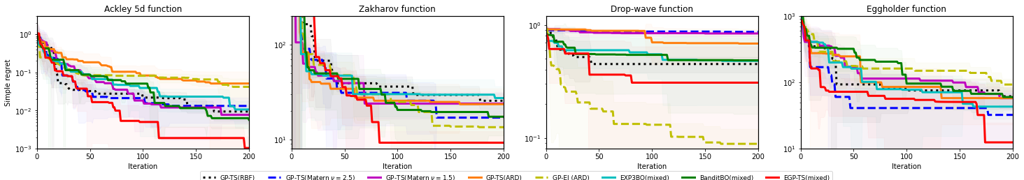
Figure 1: Simple regret on Ackley-5d, Zakharov, DropWave and Eggholder function (from left to right). Dictionary has 4 kernels with distinct forms: RBF with(out) ARD and Matérn with $\nu=1.5,2.5$.

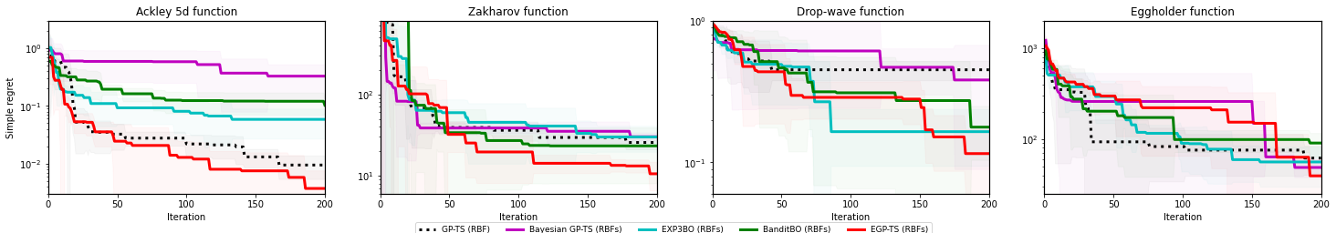
Figure 2: Simple regret on Ackley-5d, Zakharov, DropWave and Eggholder function (from left to right) using RBF kernels. Dictionary has 11 RBF kernels with lengthscales given by $\{10^{c}\}_{c=-4}^{6}$.

Theorem 1. Under Assumption 1, the cumulative Bayesian regret (13) of EGP-TS over $T$ slots, is bounded by

$$\mathcal{BR}(T)\leq c_{1}\sqrt{MT^{c+1}\log T}+2\sigma_{n}\sqrt{MT\log T}+c_{2}$$

where the constants $c_{1}\!:=\!(2\!+\!\sqrt{d})(2/\log(1\!\!+\!\!\sigma_{n}^{-2})^{1/2}$ and $c_{2}\!:=\!6MB\!+\!(\pi^{2}d)/6\!+\!\sqrt{2\pi}M/12$ ($B$ is a constant given in Lemma 3 in App. B ) are not dependent on $T$.

Proof sketch. The detailed proof of Theorem 1 is deferred to App. B. The key step in the proof builds on the connection with UCB based approaches, that is manifested via decomposing the Bayesian regret (13) as

$$\mathcal{BR}(T)\!=\underbrace{\sum_{t=1}^{T}\mathbb{E}[f(\mathbf{x}_{*})\!-\!U_{t}^{m_{*}}(\mathbf{x}_{*})]}_{\mathcal{BR}_{1}(T)}\!+\!\!\underbrace{\sum_{t=1}^{T}\mathbb{E}[U_{t}^{m_{t}}(\mathbf{x}_{t})\!-\!\!f(\mathbf{x}_{t})]}_{\mathcal{BR}_{2}(T)}$$

where $U^{m}_{t}(\mathbf{x}):=\mu_{t-1}^{m}(\mathbf{x})+\beta_{t}^{1/2}\sigma_{t-1}^{m}(\mathbf{x})$ with $\beta_{t}$ specified by  (20) in App. B, is a UCB for $f(\mathbf{x})$ under GP $m$. This decomposition of $\mathcal{BR}(T)$ holds since $\{m_{t},\mathbf{x}_{t}\}$ and $\{m_{*},\mathbf{x}_{*}\}$ are i.i.d. and $U_{t}^{m}(\mathbf{x})$ is deterministic conditioned on $\mathcal{D}_{t-1}$, yielding [40, 19],

$$\mathbb{E}_{t-1}[U_{t}^{m_{t}}(\mathbf{x}_{t})]=\mathbb{E}_{t-1}[U_{t}^{m_{*}}(\mathbf{x}_{*})],\ \ \forall t\;.$$

Then, the Bayesian regret bound of EGP-TS can be established by upper bounding ${\cal BR}_{1}(T)$ and ${\cal BR}_{2}(T)$. Since $f\sim{\cal GP}(0,\kappa^{m_{*}})$, the former can be conveniently bounded based on related works that rely on a single GP [40, 21]. Specifically, ${\cal BR}_{1}(T)$ is proved to be upper bounded by a constant, because the probability that $f(\mathbf{x}_{*})$ is larger than $U_{t}^{m_{*}}(\mathbf{x}_{*})$ across all the slots is low [21].

To further bound ${\cal BR}_{2}(T)$ involving the extra latent variable $m_{t}$ sampled from the EGP posterior (cf. (8)), we adapt the technique in [19] that constructs a confidence set $\mathcal{C}_{t}$ for the latent variable such that $m_{*}\in\mathcal{C}_{t}$ holds with high probability; see Lemma 4 in App. B. It turns out that ${\cal BR}_{2}(T)$ can also be bounded by the sum of posterior standard deviations, which further yields the upper bound given by the MIG along the lines of [44].

The proof of Theorem 1 in App. B involves an additional discretization step of $\mathcal{X}$ per step $t$, in order to cope with the continuous feasible set $\mathcal{X}$. ∎

The following two theorems further establish the cumulative Bayesian regret bounds of parallel EGP-TS in the asynchronous and synchronous settings, whose proofs are deferred to Apps. C-D.

Theorem 2 (Asynchronous parallel setting). For $K$ workers conducting parallel function evaluations asynchronously, EGP-TS under Assumption 1 incurs the following cumulative Bayesian regret over $T$ function evaluations

$$\mathcal{BR}^{\rm asy}(T)\leq c_{1}\sqrt{\!\rho_{K}MT^{c+1}\log T}\!+\!2\sigma_{n}\sqrt{\!\!MT\log T}\!+\!c_{2}.$$

Theorem 3 (Synchronous parallel setting). For $K$ workers performing $T$ function evaluations synchronously, the cumulative Bayesian regret of EGP-TS under Assumption 1 is bounded by

$$\mathcal{BR}^{\rm syn}(T)\leq \ (K\!\!-\!\!1)\sqrt{d\log(K\!\!-\!\!1)}+2\sigma_{n}\sqrt{MT\log T}+c_{2}$$

$$+c_{3}\sqrt{\rho_{K}MT^{c+1}\log T}+c_{4}\sqrt{MT^{c+1}\log(T+K-1)}$$

where the two constants are given by $c_{3}:=2(2/\log(1+\sigma_{n}^{-2})^{1/2}$, and $c_{4}:=(2d/\log(1+\sigma_{n}^{-2})^{1/2}$.

The first term of the regret bound in Theorem 2 is $\sqrt{\rho_{K}}$ times its counterpart in Theorem 1 for the sequential setting. It shall be easily verified that Bayesian regret bounds of parallel EGP-TS become equivalent to that in the sequential setting when $K=1$ with $\rho_{1}=1$. Note that the regret bounds for parallel EGP-TS here are for the number of evaluations, that will typically exceed the bound in the sequential setup. This can be certainly the other way around if the evaluation time is of interest [21]. In all the three settings, the cumulative Bayesian regret bounds of EGP-TS boil down to $\mathcal{O}(\sqrt{MT^{c+1}\log T})$ after ignoring irrelevant constants, which is sublinear in the number of evaluations when $0\leq c<1$. Hence, EGP-TS enjoys the diminishing average regret per evaluation as $T$ grows, hereby establishing convergence to the global optimum.

6 Numerical tests

In this section, the performance of the proposed EGP-TS will be tested on a set of benchmark synthetic functions, two robotic tasks and a real hyperparameter tuning task for a feedforward neural network (FNN). The competing baselines are GP-EI [20], the default method for many traditional BO problems, and TS based methods, including GP-TS with a preselected kernel type, fully Bayesian GP-TS, as well as two ensemble approaches, which are BanditBO [32], and EXP3BO [16]. It is worth mentioning that the latter two, combining multi-armed bandits and BO, are originally designed for inputs with categorical variables, but are adapted as ensemble methods here with each “arm" referring to a GP model with the same input variables. In fully Bayesian GP model where a posterior pdf is maintained for the kernel hyperparameters, TS is implemented by first drawing a sample of the kernel hyperparameters, based on which function sampling is conducted. Existing kernel selection methods for conventional GP learning operate in batch mode using a large number of samples, hence being not suitable for the low-data BO setting. For initialization in all the methods, the first $10$ evaluation pairs are randomly selected and used to obtain the kernel hyperarameters per GP by maximizing the marginal likelihood. Unless stated otherwise, the hyperparameters are refitted every $50$ iterations for EGP-TS, and every iteration for the rest of the baselines. RF approximation is leveraged by all the TS-based approaches for fairness in comparison. All the experiments are repeated $10$ times, where the average performance and the standard deviation of all competing approaches are reported. More details about the experimental setup and additional tests on EGP-EI (cf. Remark 1) can be found in App. E.

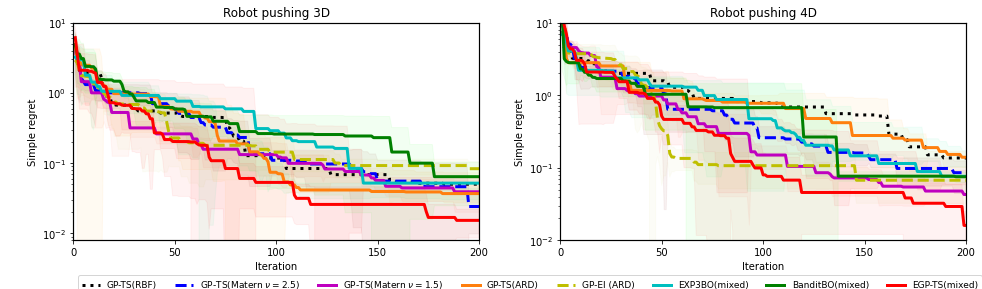
(a)

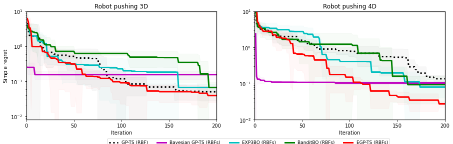
(b)

Figure 3: Simple regret on Robot pushing 3D and Robot pushing 4D tasks with dictionary (a) that has 4 kernels with distinct forms: RBF with(out) ARD and Matérn with $\nu=1.5,2.5$; and (b) that has 11 RBF kernels with characteristic lengthscales given by $\{10^{c}\}_{c=-4}^{6}$.

6.1 Tests on synthetic functions

We tested the competing methods on a suite of standard synthethic functions for BO, including Ackley-5d, Zakharov, Drop-wave as well as Eggholder, where the latter two are challenging functions with many local optima. The performance metric per slot $t$ is given by the simple regret (SR), defined as ${\cal SR}(t):=f(\mathbf{x}_{*})-\max_{\tau\in\{1,\ldots,t\}}f(\mathbf{x}_{\tau})$. First, to explore the effect of the kernel functions in the (E)GP model, we tested GP-TS with the kernel function being RBF with and without auto-relevance determination (ARD), and Matérn kernels with $\nu=1.5,2.5$. For all the ensemble methods, the kernel dictionary is comprised of the aforementioned four kernel functions. It is evident from Fig. 1 that the form of kernel function plays an important role in the performance of GP-TS. Combining different kernel functions, EGP-TS not only yields substantially improved performance relative to GP-TS counterparts, but also requires the least design efforts on the choice of the kernel function. In addition, EGP-TS achieves lower simple regret than BanditBO and EXP3BO. Although GP-EI is superior to GP-TS baselines on Zakharov function, EGP-TS yields better performance relative to the former, what demonstrates the benefit of ensembling GP models. Upon fixing the kernel type as RBF without ARD and constructing the dictionary as $11$ RBF functions with lengthscales given by $\{10^{c}\}_{c=-4}^{6}$, EGP-TS is also compared with fully Bayesian GP-based TS in addition to the aforementioned baselines. Still, EGP-TS outperforms all competitors as shown in Fig. 2. Due to space limitation, additional tests on the parallel setting are deferred to App. E.

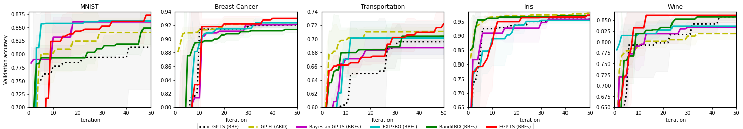
Figure 4: The best validation accuracy (so far) vs. the number of function evaluations on MNIST, Breast Cancer, Transportation, Iris, and Wine datasets (from left to right). Dictionary has 11 RBF kernels with characteristic lengthscales given by $\{10^{c}\}_{c=-4}^{6}$.

6.2 Robot pushing tasks

The second experiment concerns a practical task in robotics, where a robot adjusts its action so as to push an object towards a given goal location. By minimizing the distance between the target location and the end position of the pushed robot, we tested two scenarios with $3$ and $4$ input variables following [51]. The former optimizes the $2$-D position of the robot and the push duration, and the latter entails optimizing an additional push angle. Each scenario was repeated for $10$ randomly selected goal locations, and the average performance of the competing methods are depicted in Fig. 3. Adaptively selecting kernel function from the dictionary with $4$ distinct forms (that is, RBF with(out) ARD, and Matérn with $\nu=1.5,2.5$), the proposed EGP-TS outperforms all the competitors, including GP-EI, GP-TS with a preslected kernel, and the other two ensemble methods, as shown in Fig. 3(a). The superior performance of EGP-TS when the kernel function is fixed as RBF is also shown in Fig. 3(b), what is in accordance with Fig. 2.

6.3 Hyperparameter tuning of neural networks

The last experiment deals with hyperparameter tuning of a $2$-layer FNN with ReLU activation function for the classification task. Although this architecture does not yield the state-of-the-art classification performance, it suffices to be used to evaluate different BO methods. We tested all the competing baselines on MNIST [3], Breast cancer [1], Iris [2], Transportation [4], as well as Wine [5] datasets. Here, the kernel function is fixed to be RBF and and the dictionary of the ensemble methods is made of the aforementioned $11$ RBF kernels. For all the datasets, $70\%$ of the data are used as the training set, and the remaining are used as the validation set based on which the classification accuracy is calculated. The hyperparameters of the FNN to be tuned consist of the number of neurons per layer, the learning rate, and the batch size, whose feasible values are summarized in App. E. The best validation accuracy (so far) of the competing methods is plotted as a function of number of iterations in Fig. 4, where the proposed EGP-TS is shown to outperform the competitors on four out of the five datasets tested.

7 Conclusions

This work introduced a non-Gaussian EGP prior with adaptive kernel selection for the sought black-box function in BO. Capitalizing on the RF approximation per GP, acquisition of the subsequent query point is effected via TS, which bypasses the need for design parameters and can readily afford parallel implementation. Convergence of the proposed EGP-TS algorithm has been established by sublinear cumulative Bayesian regret in both the sequential and parallel settings. Numerical tests demonstrated the merits of EGP-TS relative to existing alternatives. Future work includes investigation of other acquisition functions based on the novel EGP surrogate model, as well as analysis via the notion of frequentist regret.

Appendix A Random feature (RF) approximation for (E)GPs and TS

A.1 RF-based GP-TS

The random feature (RF) approximation starts with a standardized shift-invariant kernel, that is, $\bar{\kappa}(\mathbf{x},\mathbf{x}^{\prime})=\bar{\kappa}(\mathbf{x}-\mathbf{x}^{\prime})$ [37]. Bochner’s theorem allows one to express any continuous $\bar{\kappa}$ as the inverse Fourier transform of a spectral density $\pi_{\bar{\kappa}}(\mathbf{v})$, expressed as [39]

$$\bar{\kappa}(\mathbf{x}-\mathbf{x}^{\prime})=\int\pi_{\bar{\kappa}}(\mathbf{v})e^{j\mathbf{v}^{\top}(\mathbf{x}-\mathbf{x}^{\prime})}d\mathbf{v}:=\mathbb{E}_{\pi_{\bar{\kappa}}}\left[e^{j\mathbf{v}^{\top}(\mathbf{x}-\mathbf{x}^{\prime})}\right]$$

where the expectation in the last equality follows since $\bar{\kappa}(\mathbf{0})=\int\pi_{\bar{\kappa}}(\mathbf{v})d\mathbf{v}=1$, thus allowing one to view $\pi_{\bar{\kappa}}$ as a pdf. For instance, if $\bar{\kappa}(\mathbf{x},\mathbf{x}^{\prime})=\exp(-\|\mathbf{x}-\mathbf{x}^{\prime}\|^{2})$, the spectral density $\pi_{\bar{\kappa}}(\mathbf{v})$ is then a standard Gaussian pdf.

Since $\bar{\kappa}$ is real, the expectation $\mathbb{E}_{\pi_{\bar{\kappa}}}$ can be rewritten as $\mathbb{E}_{\pi_{\bar{\kappa}}}\left[\cos(\mathbf{v}^{\top}(\mathbf{x}-\mathbf{x}^{\prime}))\right]$, which, upon drawing a sufficient number $D$ of independent and identically distributed (i.i.d.) samples $\{\mathbf{v}_{j}\}_{j=1}^{D}$ from $\pi_{\bar{\kappa}}(\mathbf{v})$, can be approximated by

$$\check{\bar{\kappa}}(\mathbf{x},\mathbf{x}^{\prime}):=\frac{1}{D}\sum_{j=1}^{D}\cos\left(\mathbf{v}_{j}^{\top}(\mathbf{x}-\mathbf{x}^{\prime})\right)\;.$$ (14)

Define the $2D\!\times\!1$ RF vector as [25]

$${\mbox{\boldmath$\phi$}}_{\mathbf{v}}(\mathbf{x})=\!\frac{1}{\sqrt{D}}\!\left[\sin(\mathbf{v}_{1}^{\top}\mathbf{x}),\cos(\mathbf{v}_{1}^{\top}\mathbf{x}),\ldots,\sin(\mathbf{v}_{D}^{\top}\mathbf{x}),\cos(\mathbf{v}_{D}^{\top}\mathbf{x})\right]^{\top}:$$ (15)

and use it to rewrite $\check{\bar{\kappa}}$ in (14) as $\check{\bar{\kappa}}(\mathbf{x},\mathbf{x}^{\prime})={\mbox{\boldmath$\phi$}}_{\mathbf{v}}^{\top}(\mathbf{x}){\mbox{\boldmath$\phi$}}_{\mathbf{v}}(\mathbf{x}^{\prime})$. This allows approximating the nonparametric GP prior with $\kappa=\sigma_{\theta}^{2}\bar{\kappa}$ by the linear parametric one as

$${\check{f}}(\mathbf{x})={\mbox{\boldmath$\phi$}}_{\mathbf{v}}^{\top}(\mathbf{x}){\mbox{\boldmath$\theta$}},\quad{\mbox{\boldmath$\theta$}}\sim\mathcal{N}({\mbox{\boldmath$\theta$}};\mathbf{0}_{2D},\sigma_{\theta}^{2}\mathbf{I}_{2D})\;.$$ (16)

Henceforth, the function posterior pdf can be captured by $p({\mbox{\boldmath$\theta$}}|\mathcal{D}_{t})=\mathcal{N}({\mbox{\boldmath$\theta$}};\hat{{\mbox{\boldmath$\theta$}}}_{t},{\mbox{\boldmath$\Sigma$}}_{t})$, where the first two moments are given by (${\mbox{\boldmath$\Phi$}}_{t}:=\left[{\mbox{\boldmath$\phi$}}_{\mathbf{v}}(\mathbf{x}_{1}),\ldots,{\mbox{\boldmath$\phi$}}_{\mathbf{v}}(\mathbf{x}_{t})\right]^{\top}$)

$$\hat{{\mbox{\boldmath$\theta$}}}_{t} =\left({\mbox{\boldmath$\Phi$}}_{t}^{\top}{\mbox{\boldmath$\Phi$}}_{t}+\frac{\sigma_{n}^{2}}{\sigma_{\theta}^{2}}\mathbf{I}_{2D}\right)^{-1}\!\!\!\!{\mbox{\boldmath$\Phi$}}_{t}^{\top}\mathbf{y}_{t}$$ (17a)

$${\mbox{\boldmath$\Sigma$}}_{t} =\left(\!\!\frac{{\mbox{\boldmath$\Phi$}}_{t}^{\top}{\mbox{\boldmath$\Phi$}}_{t}}{\sigma_{n}^{2}}\!+\!\frac{\mathbf{I}_{2D}}{\sigma_{\theta}^{2}}\!\!\right)^{-1}\;.$$ (17b)

With the RF-based parametric function approximant at hand, TS allows the the next query point to be selected as

$$\mathbf{x}_{t+1}=\underset{\mathbf{x}\in\mathcal{X}}{\arg\max}\ {\mbox{\boldmath$\phi$}}_{\mathbf{v}}^{\top}(\mathbf{x})\tilde{{\mbox{\boldmath$\theta$}}}_{t},\ \ \tilde{{\mbox{\boldmath$\theta$}}}_{t}\sim p({\mbox{\boldmath$\theta$}}|\mathcal{D}_{t})\;.$$ (18)

It is worth mentioning that the mean $\hat{{\mbox{\boldmath$\theta$}}}_{t}$ and covariance matrix ${\mbox{\boldmath$\Sigma$}}_{t}$ can be updated efficiently in a recursive Bayes manner with the inclusion of each new (input, evaluation) pair.

A.2 RF-based generative model in EGP

When the kernels in the dictionary of EGP are shift-invariant, the RF vector ${\mbox{\boldmath$\phi$}}_{\mathbf{v}}^{m}(\mathbf{x})$ per GP $m$ can be formed via (15) by first drawing i.i.d. random vectors $\{\mathbf{v}_{j}^{m}\}_{j=1}^{D}$ from $\pi_{\bar{\kappa}}^{m}(\mathbf{v})$, which is the spectral density of the standardized kernel $\bar{\kappa}^{m}$. Let $\sigma_{\theta^{m}}^{2}$ be the kernel magnitude so that $\kappa^{m}=\sigma_{\theta^{m}}^{2}\bar{\kappa}^{m}$. The generative model for the sought function and the noisy output $y$ per GP $m$ can be characterized through the $2D\times 1$ vector ${\mbox{\boldmath$\theta$}}^{m}$ as

$${p}({\mbox{\boldmath$\theta$}}^{m}) =\mathcal{N}({\mbox{\boldmath$\theta$}}^{m};\mathbf{0}_{2D},\sigma_{\theta^{m}}^{2}\mathbf{I}_{2D})$$

$$p(f(\mathbf{x}_{t})|i=m,{\mbox{\boldmath$\theta$}}^{m}) =\delta(f(\mathbf{x}_{t})-{\mbox{\boldmath$\phi$}}_{\mathbf{v}}^{m\top}(\mathbf{x}_{t}){\mbox{\boldmath$\theta$}}^{m})$$

$$p(y_{t}|{\mbox{\boldmath$\theta$}}^{m},\mathbf{x}_{t}) =\mathcal{N}(y_{t};{\mbox{\boldmath$\phi$}}_{\mathbf{v}}^{m\top}(\mathbf{x}_{t}){\mbox{\boldmath$\theta$}}^{m},\sigma_{n}^{2})\;.$$ (19)

Algorithm 1 EGP-TS

1:Input: Kernel dictionary $\mathcal{K}$, number $D$ of RFs, number $K$ of workers, and $w_{0}^{m}=1/M$ $\forall m$

2:Initialization:

3:Randomly evaluate $t_{0}$ points to obtain ${\cal D}_{t_{0}}$;

4:for $m=1,2,\ldots,M$ do

5:     Obtain kernel hyperparameters estimates $\hat{\boldsymbol{\alpha}}_{t_{0}}^{m}$ by maximizing the marginal likelihood;

6:     Draw $D$ random vectors $\{\mathbf{v}_{i}^{m}\}_{i=1}^{D}$ from $\pi_{\bar{\kappa}}^{m}(\mathbf{v})$ using $\hat{\boldsymbol{\alpha}}_{t_{0}}^{m}$;

7:     Obtain $w_{t_{0}}^{m}$, $\hat{{\mbox{\boldmath$\theta$}}}_{t_{0}}^{m}$, and ${\mbox{\boldmath$\Sigma$}}_{t_{0}}^{m}$ based on (7) and (17);

8:end for

9:for $t=t_{0},t_{0}+1,\ldots$ do

10:     if Reinitialization then

11:         for $m=1,2,\ldots,M$ do

12:              Obtain $\hat{\boldsymbol{\alpha}}_{t}^{m}$ by marginal likelihood maximization using ${\cal D}_{t}$;

13:              Draw $D$ random vectors $\{\mathbf{v}_{i}^{m}\}_{i=1}^{D}$ from $\pi_{\bar{\kappa}}^{m}(\mathbf{v})$ using $\hat{\boldsymbol{\alpha}}_{t}^{m}$;

14:              Obtain $w_{t}^{m}$, $\hat{{\mbox{\boldmath$\theta$}}}_{t}^{m}$, and ${\mbox{\boldmath$\Sigma$}}_{t}^{m}$ based on (7) and (17);

15:         end for

16:     end if

17:     for $k=1,2,\ldots,K$ do

18:         Sample $m_{t}^{k}$ based on pmf $\mathbf{w}_{t}$;

19:         Sample $\tilde{{\mbox{\boldmath$\theta$}}}_{t}^{k}$ from $\mathcal{N}(\hat{{\mbox{\boldmath$\theta$}}}^{m_{t}^{k}}_{t},{\mbox{\boldmath$\Sigma$}}^{m_{t}^{k}}_{t})$;

20:         Obtain $\mathbf{x}_{t+1}^{k}=\underset{\mathbf{x}\in\mathcal{X}}{\arg\max}\ \ \tilde{{\mbox{\boldmath$\theta$}}}_{t}^{k\top}\!\!{\mbox{\boldmath$\phi$}}^{m_{t}^{k}}(\mathbf{x})$;

21:         Evaluate $\mathbf{x}_{t+1}^{k}$ to obtain $y_{t+1}^{k}$;

22:     end for

23:     Update $\{w_{t+1}^{m},\hat{{\mbox{\boldmath$\theta$}}}_{t+1}^{m},{\mbox{\boldmath$\Sigma$}}_{t+1}^{m}\}_{m}$ with $\{\mathbf{x}_{t+1}^{k},y_{t+1}^{k}\}_{k}$ based on (10) and  (11);

24:     ${\cal D}_{t+1}={\cal D}_{t}\cup\{\mathbf{x}_{t+1}^{k},y_{t+1}^{k}\}_{k}$;

25:end for

Algorithm 2 Asynchronously parallel EGP-TS

1:Input: Kernel dictionary $\mathcal{K}$, number $D$ of RFs, number $K$ of workers, and $w_{0}^{m}=1/M$ $\forall m$ .

2:Initialization:

3:Randomly evaluate $t_{0}$ points to obtain ${\cal D}_{t_{0}}$;

4:for $m=1,2,\ldots,M$ do

5:     Obtain kernel hyperparameters estimates $\hat{\boldsymbol{\alpha}}_{t_{0}}^{m}$ by maximizing the marginal likelihood;

6:     Draw $D$ random vectors $\{\mathbf{v}_{i}^{m}\}_{i=1}^{D}$ from $\pi_{\bar{\kappa}}^{m}(\mathbf{v})$ using $\hat{\boldsymbol{\alpha}}_{t_{0}}^{m}$;

7:     Obtain $w_{t_{0}}^{m}$, $\hat{{\mbox{\boldmath$\theta$}}}_{t_{0}}^{m}$, and ${\mbox{\boldmath$\Sigma$}}_{t_{0}}^{m}$ based on (7) and (17);

8:end for

9:for $k=1,2,\ldots,K$ do

10:     Sample $m_{t_{0}}^{k}$ based on pmf $\mathbf{w}_{t_{0}}$;

11:     Sample $\tilde{{\mbox{\boldmath$\theta$}}}_{t_{0}}^{k}$ from $\mathcal{N}(\hat{{\mbox{\boldmath$\theta$}}}^{m_{t_{0}}^{k}}_{t_{0}},{\mbox{\boldmath$\Sigma$}}^{m_{t_{0}}^{k}}_{t_{0}})$;

12:     Obtain $\mathbf{x}_{t_{0}+1}^{k}=\underset{\mathbf{x}\in\mathcal{X}}{\arg\max}\ \ \tilde{{\mbox{\boldmath$\theta$}}}_{t_{0}}^{k\top}\!\!{\mbox{\boldmath$\phi$}}^{m_{t_{0}}^{k}}(\mathbf{x})$;

13:end for

14:for $t=t_{0}+1,\ldots$ do

15:     Wait for a worker to obtain $\{\mathbf{x}_{t},y_{t}\}$, and ${\cal D}_{t}={\cal D}_{t-1}\cup\{\mathbf{x}_{t},y_{t}\}$;

16:     if Reinitialization then

17:         for $m=1,2,\ldots,M$ do

18:              Obtain $\hat{\boldsymbol{\alpha}}_{t}^{m}$ by marginal likelihood maximization using ${\cal D}_{t}$;

19:              Draw $D$ random vectors $\{\mathbf{v}_{i}^{m}\}_{i=1}^{D}$ from $\pi_{\bar{\kappa}}^{m}(\mathbf{v})$ using $\hat{\boldsymbol{\alpha}}_{t}^{m}$;

20:              Obtain $w_{t}^{m}$, $\hat{{\mbox{\boldmath$\theta$}}}_{t}^{m}$, and ${\mbox{\boldmath$\Sigma$}}_{t}^{m}$ based on (7) and (17);

21:         end for

22:     else

23:         Obtain updated $\{w_{t}^{m},\hat{{\mbox{\boldmath$\theta$}}}_{t}^{m},{\mbox{\boldmath$\Sigma$}}_{t}^{m}\}_{m}$ using $\{\mathbf{x}_{t},y_{t}\}$ based on (10) and  (11);

24:     end if

25:     Sample $m_{t}$ based on pmf $\mathbf{w}_{t}$;

26:     Sample $\tilde{{\mbox{\boldmath$\theta$}}}_{t}$ from $\mathcal{N}(\hat{{\mbox{\boldmath$\theta$}}}^{m_{t}}_{t},{\mbox{\boldmath$\Sigma$}}^{m_{t}}_{t})$;

27:     Obtain $\mathbf{x}_{t+1}=\underset{\mathbf{x}\in\mathcal{X}}{\arg\max}\ \ \tilde{{\mbox{\boldmath$\theta$}}}_{t}^{\top}\!\!{\mbox{\boldmath$\phi$}}^{m_{t}}(\mathbf{x})$;

28:     Assign $\mathbf{x}_{t+1}$ to the worker to evaluate;

29:end for

Appendix B Proof of Theorem 1

Before performing the Bayesian regret analysis for EGP-TS, the following lemma will be first presented.

Lemma 3. (Supremum of a GP sample path [6]). If $f\sim{\cal GP}(0,\kappa^{m})$ is a continuous sample path for any $m\in\mathcal{M}$, then $\mathbb{E}[\|f\|_{\infty}]=B<\infty$, and further

$$\underset{\mathbf{x}\in\mathcal{X}}{\max}|f(\mathbf{x}_{*})-f(\mathbf{x})|\leq 2B\;.$$

Lemma  3 holds when kernels are twice differentiable - what is readily satisfied under Assumption 1.

To bound the cumulative Bayesian regret of EGP-TS, we will rely on its link with the corresponding upper confidence bound algorithm in [40]. Conditioned on GP model $m$ and past data $\mathcal{D}_{t-1}$, the high probability upper confidence bound for $f(\mathbf{x})$ is given by $U^{m}_{t}(\mathbf{x}):=\mu_{t-1}^{m}(\mathbf{x})+\beta_{t}^{1/2}\sigma_{t-1}^{m}(\mathbf{x})$, where $\beta_{t}:=2\log(t^{2}|\mathcal{X}_{t}|)$. Here, $\mathcal{X}_{t}$ is obtained by discretizing each dimension of $\mathcal{X}$ using $n_{t}=t^{2}dab\sqrt{\pi}$ equally spaced grid points. Thus, $|\mathcal{X}_{t}|=(n_{t})^{d}$, and

$$\beta_{t}=4(d+1)\log t+2d\log(dab\sqrt{\pi})\approx d\log t\;.$$ (20)

With $[\mathbf{x}]_{t}$ representing the closest point to $\mathbf{x}$ in $\mathcal{X}_{t}$, it can be easily verified that

$$\|\mathbf{x}-[\mathbf{x}]_{t}\|_{1}\leq d/n_{t},\ \ \forall\mathbf{x}\in\mathcal{X}.$$ (21)

Consider next the following decomposition

$$\mathcal{BR}(T) :=\sum_{t=1}^{T}\mathbb{E}[f(\mathbf{x}_{*})-f(\mathbf{x}_{t})]$$

$$\overset{(a)}{=}\underbrace{\sum_{t=1}^{T}\mathbb{E}\left[f(\mathbf{x}_{*})-f([\mathbf{x}_{*}]_{t})\right]}_{:=A_{1}}+\underbrace{\sum_{t=1}^{T}\mathbb{E}\left[f([\mathbf{x}_{*}]_{t}-U_{t}^{m_{*}}([\mathbf{x}_{*}]_{t})\right]}_{:=A_{2}}$$

$$\qquad+\underbrace{\sum_{t=1}^{T}\mathbb{E}\left[U_{t}^{m_{*}}([\mathbf{x}_{*}]_{t})-U_{t}^{m_{t}}([\mathbf{x}_{t}]_{t})\right]}_{:=A_{3}}+\underbrace{\sum_{t=1}^{T}\mathbb{E}\left[U_{t}^{m_{t}}([\mathbf{x}_{t}]_{t})-f([\mathbf{x}_{t}]_{t})\right]}_{:=A_{4}}$$

$$\qquad+\underbrace{\sum_{t=1}^{T}\mathbb{E}\left[f([\mathbf{x}_{t}]_{t})-f(\mathbf{x}_{t})\right]}_{:=A_{5}}\;.$$ (22)

Since $\{\mathbf{x}_{t},m_{t}\}$ and $\{\mathbf{x}_{*},m_{*}\}$ are identically distributed given $\mathcal{D}_{t-1}$, the fact that $U_{t}^{m}(\mathbf{x})$ is a deterministic function of $\mathcal{D}_{t-1}$ yields $A_{3}=0$ [40, 19].

Next, we will provide an upper bound for $A_{1}$ and $A_{5}$ following the proof in [21]. Letting $L_{\max}=\underset{j=\{1,\ldots,d\}}{\sup}\ \ \underset{\mathbf{x}\in\mathcal{X}}{\sup}\left|\frac{\partial f(\mathbf{x})}{\partial x_{j}}\right|$, the union bound under Assumption 1 implies that

$${\rm Pr}(L_{\max}\geq c)\leq dae^{-(c/b)^{2}}$$

which allows us to obtain

$$\mathbb{E}[|f(\mathbf{x})-f([\mathbf{x}]_{t})|] \leq\mathbb{E}[L\|\mathbf{x}-[\mathbf{x}]_{t}\|_{1}]\overset{(a)}{\leq}\frac{d}{n_{t}}\mathbb{E}[L_{\rm max}]\overset{(b)}{=}\frac{d}{n_{t}}\int_{c=0}^{\infty}{\rm Pr}(L_{\rm max}\geq c)dc$$

$$\leq\frac{d}{n_{t}}\int_{c=0}^{\infty}dae^{-(c/b)^{2}}dc=\frac{\sqrt{\pi}d^{2}ab}{2n_{t}}=\frac{d}{2t^{2}}$$

where $(a)$ results from (21), and $(b)$ utilizes for $L_{\rm max}\geq 0$ the equality $\mathbb{E}[L_{\rm max}]=\int_{c=0}^{\infty}{\rm Pr}(L_{\rm max}\geq c)dc$. Hence, $A_{1}$ and $A_{5}$ are bounded by

$$A_{1}=A_{5}\leq\sum_{t=1}^{T}\frac{d}{2t^{2}}\leq\frac{\pi^{2}d}{12}\;.$$ (23)

Further, $A_{2}$ can be upper bounded as

$$A_{2} \leq\sum_{t=1}^{T}\mathbb{E}\left[\mathbb{I}(f([\mathbf{x}_{*}]_{t})>U_{t}^{m_{*}}([\mathbf{x}_{*}]_{t}))\left[f([\mathbf{x}_{*}]_{t}-U_{t}^{m_{*}}([\mathbf{x}_{*}]_{t})\right]\right]$$

$$\leq\sum_{t=1}^{T}\sum_{m\in\mathcal{M}}\sum_{\mathbf{x}\in\mathcal{X}_{t}}\mathbb{E}\left[\mathbb{I}(f(\mathbf{x})>U_{t}^{m}(\mathbf{x}))\left[f(\mathbf{x})-U_{t}^{m}(\mathbf{x})\right]\right]$$

$$\overset{(a)}{=}\sum_{t=1}^{T}\sum_{m\in\mathcal{M}}\sum_{\mathbf{x}\in\mathcal{X}_{t}}\frac{\sigma_{t-1}^{m}(\mathbf{x})}{\sqrt{2\pi}t^{2}|\mathcal{X}_{t}|}$$

$$\overset{(b)}{\leq}\sum_{t=1}^{T}\sum_{m\in\mathcal{M}}\sum_{\mathbf{x}\in\mathcal{X}_{t}}\frac{1}{\sqrt{2\pi}t^{2}|\mathcal{X}_{t}|}=\frac{\sqrt{2\pi}M}{12}$$ (24)

where, since $f(\mathbf{x})-U_{t}^{m}(\mathbf{x})|\mathcal{D}_{t-1}\sim\mathcal{N}\left(-\beta_{t}^{1/2}\sigma_{t-1}^{m}(\mathbf{x}),(\sigma_{t-1}^{m}(\mathbf{x}))^{2}\right)$, $(a)$ holds using the identity $\mathbb{E}[r\mathbb{I}(r>0)]=\frac{\sigma}{\sqrt{2\pi}}\exp(-\frac{\mu^{2}}{2\sigma^{2}})$ if $r\sim\mathcal{N}(\mu,\sigma^{2})$ and $\mu<0$. Inequality $(b)$ is simply due to $\sigma_{t-1}^{m}(\mathbf{x})\leq 1$.

The last step is to upper bound $A_{4}$, by constructing a confidence set $\mathcal{C}_{t}$ for the latent state per slot $t$ so that $m_{*}\in\mathcal{C}_{t}$ holds with high probability [19]. We will replace $[\mathbf{x}_{t}]_{t}$ by $\mathbf{x}_{t}$ for notational brevity, given that the following result holds for both cases. Consider $\mathcal{C}_{t}:=\{m\in\mathcal{M}:G_{t}^{m}\leq 2\sigma_{n}\sqrt{N_{t-1}^{m}\log T}\}$, where $N_{t-1}^{m}=\sum_{\tau=1}^{t-1}\mathbb{I}(m_{\tau}=m)$, and

$$G_{t}^{m}:=\sum_{\tau=1}^{t-1}\mathbb{I}(m_{\tau}=m)\left(L_{\tau}^{m}(\mathbf{x}_{\tau})-y_{\tau}\right)\;.$$ (25)

Here, $L_{t}^{m}(\mathbf{x})=\mu_{t-1}^{m}(\mathbf{x})-\eta\sigma^{m}_{t-1}(\mathbf{x})$ with $\eta=2\sqrt{\log T}$ is a lower confidence bound for $f(\mathbf{x})$ conditioned on model $m$. For later use, we will first present the following two lemmas, whose proofs are deferred to Secs. B.1-2.

Lemma 4. It holds that ${\rm Pr}(m_{*}\notin\mathcal{C}_{t}|\mathcal{D}_{t-1})\leq 2MT^{-1},\forall t\in\mathcal{T}:=\{1,\ldots,T\}$.

Lemma 5. It holds that $\mathbb{E}\left[\mu_{t-1}^{m_{t}}(\mathbf{x}_{t})-f(\mathbf{x}_{t})\right]<2B,\forall m_{t}\in\mathcal{M},\mathbf{x}_{t}\in\mathcal{X},t\in{\cal T}.$

The following decomposition will be applied towards bounding $A_{4}$

$$A_{4} =\mathbb{E}\left[\sum_{t=1}^{T}\left(U_{t}^{m_{t}}(\mathbf{x}_{t})-\mu_{t-1}^{m_{t}}(\mathbf{x}_{t})\right)\right]+\mathbb{E}\left[\sum_{t=1}^{T}\left(\mu_{t-1}^{m_{t}}(\mathbf{x}_{t})-f(\mathbf{x}_{t})\right)\right]$$

$$\leq\underbrace{\sum_{t=1}^{T}\mathbb{E}[\beta_{t}^{1/2}\sigma^{m_{t}}_{t-1}(\mathbf{x}_{t})]}_{:=A_{4,1}}+\underbrace{\sum_{t=1}^{T}\mathbb{E}\left[\left(\mu_{t-1}^{m_{t}}(\mathbf{x}_{t})-f(\mathbf{x}_{t})\right)\mathbb{I}(m_{t}\in\mathcal{C}_{t})\right]}_{:=A_{4,2}}$$

$$\qquad+\underbrace{\sum_{t=1}^{T}\mathbb{E}\left[2B\mathbb{I}(m_{t}\not\in\mathcal{C}_{t})\right]}_{:=A_{4,3}}$$ (26)

where the last inequality holds based on Lemma 5.

As $m_{*}$ and $m_{t}$ are identically distributed given $\mathcal{D}_{t-1}$ [40, 19], Lemma 4 allows $A_{4,3}$ to be readily bounded by

$$A_{4,3}=2B\sum_{t=1}^{T}\mathbb{E}[\mathbb{I}(m_{*}\not\in\mathcal{C}_{t})]\leq 4MB\;.$$ (27)

Meanwhile, we have that

$$A_{4,2} =\sum_{t=1}^{T}\mathbb{E}\left[\left(\mu_{t-1}^{m_{t}}(\mathbf{x}_{t})\!-\!L_{t}^{m_{t}}(\mathbf{x}_{t})\right)\mathbb{I}(m_{t}\in\mathcal{C}_{t})\right]\!+\!\sum_{t=1}^{T}\mathbb{E}\left[\left(L_{t}^{m_{t}}(\mathbf{x}_{t})\!-\!y_{t}\right)\mathbb{I}(m_{t}\in\mathcal{C}_{t})\right]$$

$$\overset{(a)}{\leq}\sum_{t=1}^{T}\mathbb{E}[\eta\sigma^{m_{t}}_{t-1}(\mathbf{x}_{t})]+\sum_{m\in\mathcal{M}}\mathbb{E}[G_{t_{\rm max}^{m}}^{m}]+2MB$$

$$\overset{(b)}{\leq}\sum_{t=1}^{T}\mathbb{E}[\eta\sigma^{m_{t}}_{t-1}(\mathbf{x}_{t})]+\sum_{m\in\mathcal{M}}\mathbb{E}[2\sigma_{n}\sqrt{N_{T}^{m}\log T}]+2MB$$

$$\overset{(c)}{\leq}\sum_{t=1}^{T}\mathbb{E}[\eta\sigma^{m_{t}}_{t-1}(\mathbf{x}_{t})]+2\sigma_{n}\sqrt{MT\log T}+2MB\;.$$ (28)

where, with $t_{\rm max}^{m}$ being the last slot that $m$ is selected, $(a)$ holds by leveraging the definition of $G_{t_{\rm max}^{m}}^{m}$ and bounding the $L_{t_{\rm max}^{m}}^{m}(\mathbf{x})-y_{t_{\rm max}^{m}}$ by $2B$; $(b)$ comes from the definition of $\mathcal{C}_{t}$; and, $(c)$ leverages Cauchy-Schwarz inequality to yield

$$\sum_{m=1}^{M}\sqrt{N_{T}^{m}}\leq\sqrt{M\sum_{m=1}^{M}N_{T}^{m}}=\sqrt{MT}\;.$$ (29)

Putting together the bounds for $A_{1}-A_{5}$, the cumulative Bayesian regret of EGP-TS over $T$ evaluations is bounded by

$${\cal BR}(T) \leq(\eta+\beta_{T}^{1/2})\sum_{t=1}^{T}\mathbb{E}[\sigma^{m_{t}}_{t-1}(\mathbf{x}_{t})]+2\sigma_{n}\sqrt{MT\log T}+6MB+\frac{\pi^{2}d}{6}+\frac{\sqrt{2\pi}M}{12}$$ (30)

where the first term can be bounded with $\mathcal{T}_{T}^{m}:=\{t\in\mathcal{T}:m_{t}=m\}$ and $T_{m}:=|\mathcal{T}_{T}^{m}|$as

$$\sum_{t=1}^{T}\mathbb{E}[\sigma^{m_{t}}_{t-1}(\mathbf{x}_{t})] \leq\sum_{m=1}^{M}\mathbb{E}\left[\sum_{t\in\mathcal{T}_{T}^{m}}\sigma^{m}_{t-1}(\mathbf{x}_{t})\right]\overset{(a)}{\leq}\sum_{m=1}^{M}\mathbb{E}\left[\sum_{t=1}^{T_{m}}\sigma^{m}_{t-1}(\mathbf{x}_{t})\right]$$

$$\overset{(b)}{\leq}\sum_{m=1}^{M}\mathbb{E}\left(T_{m}\sum_{t=1}^{T_{m}}\left(\sigma_{t-1}^{m}(\mathbf{x}_{t})\right)^{2}\right)^{1/2}\overset{(c)}{\leq}\sum_{m=1}^{M}\left(\frac{2{T_{m}}\gamma_{T_{m}}}{\log\left(1+\sigma_{n}^{-2}\right)}\right)^{1/2}$$

$$\overset{(d)}{\leq}\sum_{m=1}^{M}\left(\frac{2T_{m}^{1+c}}{\log\left(1+\sigma_{n}^{-2}\right)}\right)^{1/2}\overset{(e)}{\leq}\left(\frac{2MT^{1+c}}{\log\left(1+\sigma_{n}^{-2}\right)}\right)^{1/2}$$ (31)

where $(a)$ holds since $\sigma_{t}^{m}(\mathbf{x})$ decreases as $t$ grows; $(b)$ is due to the Cauchy-Schwarz inequality; $(c)$ leverages Lemmas 5.3 and 5.4 of [44] that bound the sum of posterior variances via the MIG; $(d)$ follows upon bounding $\gamma_{T_{m}}$ using Lemma 1; and, $(e)$ holds upon utilizing the following inequality based on Cauchy-Schwarz inequality

$$\sum_{m=1}^{M}\left(T_{m}^{1+c}\right)^{1/2}\leq\left(M\sum_{m=1}^{M}T_{m}^{1+c}\right)^{1/2}\leq\left(M\left(\sum_{m=1}^{M}T_{m}\right)^{1+c}\right)^{1/2}=\left(MT^{1+c}\right)^{1/2}.$$

Upon plugging in (31) into (30), Theorem 1 holds with $\eta=2\sqrt{\log T}$ and $\beta_{T}^{1/2}\approx\sqrt{d\log T}$.

B.1 Proof for Lemma 4

For $m_{*}\in\mathcal{M}$, define the following event at slot $t$

$$\mathcal{E}_{t}^{m_{*}}:=\{|f(\mathbf{x})-\mu^{m_{*}}_{t-1}(\mathbf{x})|\leq\eta\sigma_{t-1}^{m_{*}}(\mathbf{x})\}$$ (32)

the collection of which over $T$ slots is $\mathcal{E}^{m_{*}}_{1:T}:=\cap_{t=1}^{T}\mathcal{E}_{t}^{m_{*}}$. With $\bar{\mathcal{E}}^{m_{*}}_{1:T}$ representing its complement, it follows that

$$\mathbb{E}[I(\bar{\mathcal{E}}^{m_{*}}_{1:T})] \leq\sum_{t=1}^{T}\sum_{m\in\mathcal{M}}\mathbb{E}\left[\mathbb{E}_{t-1}[\mathbb{I}(\bar{\mathcal{E}}^{m}_{t})]\right]$$ (33)

$$=\sum_{t=1}^{T}\sum_{m\in\mathcal{M}}\mathbb{E}\left[{\rm Pr}_{t-1}\left(|\mu^{m}_{t-1}(\mathbf{x})-f(\mathbf{x})|>\eta\sigma_{t-1}^{m}(\mathbf{x})\right)\right]\overset{(a)}{\leq}MT^{-1}$$

where $(a)$ comes from the inequality ${\rm Pr}(|r|>\eta)\leq e^{-\eta^{2}/2}$ with $r=|\mu^{m}_{t-1}(\mathbf{x})-f(\mathbf{x})|/\sigma_{t-1}^{m}(\mathbf{x})\sim\mathcal{N}(0,1)$ and $\eta=2\sqrt{\log T}$.

Since $n_{\tau}=f(\mathbf{x}_{\tau})-y_{\tau}\sim\mathcal{N}(0,\sigma_{n}^{2})$, $\{n_{\tau}\}_{\tau\in\mathcal{T}_{t}^{m}}$ is then a martingale difference sequence w.r.t. $\{\mathcal{D}_{\tau}\}_{\tau\in\mathcal{T}_{t}^{m}}$, where $\mathcal{T}_{t}^{m}:=\{\tau|m_{\tau}=m,\tau\in\{1,\ldots,t\}\}$.

$$G_{t}^{m}I(\mathcal{E}^{m}_{1:T}) =\sum_{\tau\in\mathcal{T}_{t}^{m}}(L_{\tau}^{m}(\mathbf{x}_{\tau})-y_{\tau})\mathbb{I}(|f(\mathbf{x}_{\tau})-\mu^{m}_{\tau-1}(\mathbf{x}_{\tau})|\leq\eta\sigma_{\tau-1}^{m}(\mathbf{x}_{\tau}))$$

$$=\sum_{\tau\in\mathcal{T}_{t}^{m}}(L_{\tau}^{m}(\mathbf{x}_{\tau})-y_{\tau})\mathbb{I}(L_{\tau}^{m}(\mathbf{x}_{\tau})<f(\mathbf{x}_{\tau}))\leq\sum_{\tau\in\mathcal{T}_{t}^{m}}n_{\tau}\;.$$ (34)

For any $m\in\mathcal{M}$ and $t\in\mathcal{T}$, $u=|\mathcal{T}_{t}^{m}|$ is random and takes value from $\{1,\ldots,t-1\}$. For any $u$, Azuma’s inequality yields

$${\rm Pr}_{t-1}(G_{t}^{m}I(\mathcal{E}^{m}_{1:T})\geq 2\sigma_{n}\sqrt{u\log T}) \leq{\rm Pr}\left(\sum_{\tau\in\mathcal{T}_{t}^{m}}n_{\tau}\geq 2\sigma_{n}\sqrt{u\log T}\right)$$

$$\leq\exp(-2\log T)=T^{-2}$$ (35)

based on which, we arrive at

$${\rm Pr}_{t}(m_{*}\not\in\mathcal{C}_{t})\leq\sum_{m\in\mathcal{M}}\sum_{u=1}^{t-1}{\rm Pr}(G_{t}^{m}\geq 2\sigma_{n}\sqrt{u\log T})$$ (36)

$$\leq\sum_{m\in\mathcal{M}}\sum_{u=1}^{t-1}\mathbb{E}\left[{\rm Pr}_{t-1}\left(G_{t}^{m}\mathbb{I}(\mathcal{E}^{m}_{1:T})\geq 2\sigma_{n}\sqrt{u\log T}\right)\right]+{\rm Pr}(\bar{\mathcal{E}}^{m_{*}}_{1:T})\leq 2MT^{-1}\;.$$

thus finalizing the proof of Lemma 4.

B.2 Proof for Lemma 5

Since $\{\mathbf{x}_{t},m_{t}\}$ and $\{\mathbf{x}_{*},m_{*}\}$ are identically distributed conditioned on $\mathcal{D}_{t-1}$, it holds that

$$\mathbb{E}[\mu_{t-1}^{m_{t}}(\mathbf{x}_{t})]=\mathbb{E}[\mathbb{E}_{t-1}[\mu_{t-1}^{m_{t}}(\mathbf{x}_{t})]]=\mathbb{E}[\mathbb{E}_{t-1}[\mu_{t-1}^{m_{*}}(\mathbf{x}_{*})]]=\mathbb{E}[\mu_{t-1}^{m_{*}}(\mathbf{x}_{*})]\;.$$

Further, the identity $\mathbb{E}_{t-1}[\mu_{t-1}^{m_{*}}(\mathbf{x}_{*})]=\mathbb{E}_{t-1}[f(\mathbf{x}_{*})]$ with $f\sim{\cal GP}(0,\kappa^{m_{*}})$, yields the following result

$$\mathbb{E}\left[\mu_{t-1}^{m_{t}}(\mathbf{x}_{t})\!-\!f(\mathbf{x}_{t})\right] =\mathbb{E}\left[\mu_{t-1}^{m_{t}}(\mathbf{x}_{t})\!-\!\mu_{t-1}^{m_{*}}(\mathbf{x}_{*})\!+\!\mu_{t-1}^{m_{*}}(\mathbf{x}_{*})-f(\mathbf{x}_{*})\!+\!f(\mathbf{x}_{*})\!-\!f(\mathbf{x}_{t})\right]$$

$$=\mathbb{E}[f(\mathbf{x}_{*})-f(\mathbf{x}_{t})]\leq 2B$$

where, thanks to Lemma 3, the last inequality holds.

Appendix C Proof of Theorem 2

For the asynchronous parallel setting, the upper confidence bound for the $t$th function evaluation is given by

$$\bar{U}_{t}^{m}(\mathbf{x}):=\mu_{\mathcal{D}_{t-1}}^{m}(\mathbf{x})+\beta_{t}^{1/2}\sigma_{\mathcal{D}_{t-1}}^{m}(\mathbf{x})$$ (37)

where $\mathcal{D}_{t-1}$ contains all the acquired data before evaluation index $t$ is assigned. Here, $|\mathcal{D}_{t-1}|=t-K$ for $t>K$, and $|\mathcal{D}_{t-1}|=0$ for $t\leq K$.

Leveraging a decomposition similar to that in (22), $A_{1}$–$A_{3}$ and $A_{5}$ could be derived as in Sec. A. Upon replacing the subscript $t-1$ of $\mu$ and $\sigma$ by $\mathcal{D}_{t-1}$, the term $A_{4}$ can be bounded as in (26), that is

$$A_{4} \leq\sum_{t=1}^{T}\mathbb{E}[(\beta_{t}^{1/2}+\eta)\sigma^{m_{t}}_{\mathcal{D}_{t-1}}(\mathbf{x}_{t})]+2\sigma_{n}\sqrt{MT\log T}+6MB$$ (38)

where the first term can be further bounded based on Lemma 2 and (31) as

$$\sum_{t=1}^{T}\mathbb{E}[(\beta_{t}^{1/2}+\eta)\sigma^{m_{t}}_{\mathcal{D}_{t-1}}(\mathbf{x}_{t})] \overset{(a)}{\leq}(\beta_{T}^{1/2}+\eta)\sum_{t=1}^{T}\mathbb{E}[\rho_{K}^{1/2}\sigma^{m_{t}}_{t-1}]$$

$$\leq(2+\sqrt{d})\left(\frac{2\rho_{K}MT^{c+1}\log T}{\log\left(1+\sigma_{n}^{-2}\right)}\right)^{1/2}\;.$$ (39)

Thus, the cumulative Bayesian regret for parallel EGP-TS in the asynchronous setup can be established as in Theorem 2.

Appendix D Proof of Theorem 3

The proof of Theorem 3 entails introducing

$$V_{t}^{m}(\mathbf{x}):=\mu_{\mathcal{D}_{t-1}}^{m}(\mathbf{x})+\beta_{t+K-1}^{1/2}\sigma_{t-1}^{m}(\mathbf{x})$$ (40)

based on which the cumulative Bayesian regret can be decomposed after using (37) as (cf. (22))

$$\mathcal{BR}^{\rm syn}(T):=\sum_{t=1}^{T}\mathbb{E}[f(\mathbf{x}_{*})-f(\mathbf{x}_{t})]$$ (41)

$$\overset{(a)}{=}\underbrace{\sum_{t=1}^{T}\mathbb{E}\left[f(\mathbf{x}_{*})-f([\mathbf{x}_{*}]_{t})\right]}_{:=C_{1}}+\underbrace{\sum_{t=1}^{T}\mathbb{E}\left[f([\mathbf{x}_{*}]_{t}-\bar{U}_{t}^{m_{*}}([\mathbf{x}_{*}]_{t})\right]}_{:=C_{2}}$$

$$\qquad+\underbrace{\sum_{t=1}^{T}\mathbb{E}\left[\bar{U}_{t}^{m_{*}}([\mathbf{x}_{*}]_{t})-V_{t}^{m_{*}}([\mathbf{x}_{*}]_{t})\right]}_{:=C_{3}}+\underbrace{\sum_{t=1}^{T}\mathbb{E}\left[V_{t}^{m_{*}}([\mathbf{x}_{*}]_{t})-V_{t}^{m_{t}}([\mathbf{x}_{t}]_{t})\right]}_{:=C_{4}}$$

$$\qquad+\underbrace{\sum_{t=1}^{T}\mathbb{E}\left[V_{t}^{m_{t}}([\mathbf{x}_{t}]_{t})-f([\mathbf{x}_{t}]_{t})\right]}_{:=C_{5}}+\underbrace{\sum_{t=1}^{T}\mathbb{E}\left[f([\mathbf{x}_{t}]_{t})-f(\mathbf{x}_{t})\right]}_{:=C_{6}}\;.$$

As with the proof of Theorem 1, it follows that

$$C_{1}=C_{6}\leq\frac{\pi^{2}d}{12},\quad C_{4}=0,\quad C_{2}\leq\frac{\sqrt{2\pi}M}{12}.$$ (42)

Next, we will further bound $C_{3}$ and $C_{5}$, starting with

$$C_{3} =\sum_{t=1}^{K-1}\beta_{t}^{1/2}\mathbb{E}[\sigma^{m_{*}}_{{\cal D}_{t-1}}([\mathbf{x}_{*}]_{t})]-\sum_{T-K+1}^{T}\beta_{t+M-1}^{1/2}\mathbb{E}[\sigma^{m_{*}}_{t-1}([\mathbf{x}_{*}]_{t})]$$

$$\ \ \ +\sum_{t=K}^{T-K}\beta_{t}^{1/2}\mathbb{E}[\sigma^{m_{*}}_{{\cal D}_{t-1}}([\mathbf{x}_{*}]_{t})-\sigma^{m_{*}}_{t-K}([\mathbf{x}_{*}]_{t})]\overset{(a)}{\leq}(K-1)\beta_{K-1}^{1/2}$$ (43)

where $(a)$ holds since $\sigma^{m_{*}}_{{\cal D}_{t-1}}([\mathbf{x}_{*}]_{t})\leq\sigma^{m_{*}}_{t-K}([\mathbf{x}_{*}]_{t})$, and $0<\sigma^{m_{*}}_{t}(\mathbf{x})\leq 1$.

Lastly, $C_{5}$ can be bounded as

$$C_{5} =\mathbb{E}\left[\sum_{t=1}^{T}\left(V_{t}^{m_{t}}(\mathbf{x}_{t})-\mu_{\mathcal{D}_{t-1}}^{m_{t}}(\mathbf{x}_{t})\right)\right]+\mathbb{E}\left[\sum_{t=1}^{T}\left(\mu_{\mathcal{D}_{t-1}}^{m_{t}}(\mathbf{x}_{t})-f(\mathbf{x}_{t})\right)\right]$$

$$\leq\sum_{t=1}^{T}\mathbb{E}[\beta_{t+K-1}^{1/2}\sigma^{m_{t}}_{t-1}(\mathbf{x}_{t})]+\sum_{t=1}^{T}\mathbb{E}\left[\left(\mu_{\mathcal{D}_{t-1}}^{m_{t}}(\mathbf{x}_{t})-f(\mathbf{x}_{t})\right)\mathbb{I}(m_{t}\in\mathcal{C}_{t})\right]$$

$$\qquad+\sum_{t=1}^{T}\mathbb{E}\left[2B\mathbb{I}(m_{t}\not\in\mathcal{C}_{t})\right]$$

$$\leq\sum_{t=1}^{T}\mathbb{E}[\beta_{t+K-1}^{1/2}\sigma^{m_{t}}_{t-1}(\mathbf{x}_{t})+\eta\sigma^{m_{t}}_{\mathcal{D}_{t-1}}(\mathbf{x}_{t})]+2\sigma_{n}\sqrt{MT\log T}+6MB$$

$$\leq\sum_{t=1}^{T}\mathbb{E}[\beta_{T+K-1}^{1/2}\sigma^{m_{t}}_{t-1}(\mathbf{x}_{t})+\eta\rho_{K}^{1/2}\sigma^{m_{t}}_{t-1}(\mathbf{x}_{t})]+2\sigma_{n}\sqrt{MT\log T}+6MB$$ (44)

which, based on the derivation of (31), and the bounds of other factors, yields the regret bound in Theorem 3.

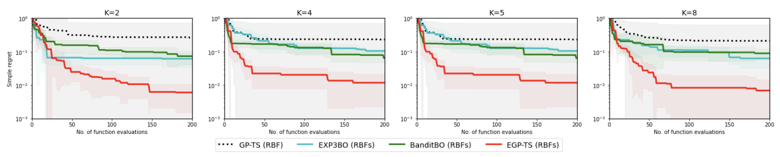
Figure 5: Simple regret for the parallel setting for various $K$s on Ackley-5d function. Dictionary has 11 RBF kernels with characteristic lengthscales given by $\{10^{c}\}_{c=-4}^{6}$.

Table 1: Feasible set of $\mathbf{x}$, maximizer $\mathbf{x}_{*}$, and $f(\mathbf{x}_{*})$ for the synthetic functions

Synthetic function	${\cal X}$	${\bf x}_{*}$	$f(\bf x_{*})$
Ackley-5d	$[0,1]^{5}$	[0.6231,0.6231,1,0.6231,0.6231]	4.6930
Zakharov	$[-5,10]^{4}$	[0,0,0,0]	0
Drop-wave	$[-5.12,5.12]^{2}$	[0,0]	1
Eggholder	$[-512,512]^{2}$	[512, 404.2319]	959.6407

Appendix E Additional details on the experiments

In this section, some additional details for the experimental setup are provided as follows.

• The kernel hyperparameters per GP for all the TS-based methods other than fully Bayesian GP-TS are obtained by maximizing the marginal likelihood using sklearn. GP-EI is implemented using BoTorch with the ARD kernel, whose hyperparameters are refitted each iteration.

• The fully Bayesian GP-TS hinges on a pre-defined kernel type where the kernel hyperparameters are assumed to be random variables. In the present work, the RBF kernel is considered and a uniform prior is assumed for the amplitude $\sigma_{\theta}^{2}$, characteristic lengthscale and noise variance $\sigma_{n}^{2}$, within intervals $[1,100],[10^{-3},10^{3}]$ and $[0.1,0.3]$ respectively. The fully Bayesian GP-TS was implemented using gpytorch and pyro Python packages.

• The per-GP prior weight is set as uniform, i.e., $w_{0}^{m}=1/M\ \forall m$.

• The number $D$ of spectral features in (14) is chosen to be $50$ in the RF vector.

• In practise, the weights may concentrate in one GP, that is, $w_{t}^{m}\approx 1$ and $w_{t}^{m^{\prime}}\approx 0$ $\forall m^{\prime}\neq m$. To encourage exploration among GP models other than $m$, one could assign a low weight, say $10^{-4}$, to GP $m^{\prime}$ $\forall m^{\prime}\neq m$.

Synthetic functions. The analytical expressions of the evaluated synthetic functions are as follows:

• Ackley-5d: $f({\bf x})=-20\exp(-0.2(\sum_{i=1}^{5}x_{i}^{2}/5)^{1/2})-\exp(\sum_{i=1}^{5}\cos(2\pi x_{i})/5)+20+e^{1}$

• Zakharov: $f({\bf x})=-\sum_{i=1}^{d}x_{i}^{2}-\left(\sum_{i=1}^{d}0.5ix_{i}\right)^{2}-\left(\sum_{i=1}^{d}0.5ix_{i}\right)^{4}$

• Drop-wave: $f({\bf x})=(1+\cos(12\sqrt{x_{1}^{2}+x_{2}^{2}}))/(0.5(x_{1}^{2}+x_{2}^{2})+2)$

• Eggholder: $f({\bf x})=(x_{2}+47)\sin\sqrt{|x_{2}+x_{1}/2+47|}+x_{1}\sin\sqrt{|x_{1}-x_{2}-47|}$

where the candidate values of $\mathbf{x}$, the corresponding optimizer $\mathbf{x}_{*}$, as well as maximum function value $f(\mathbf{x}_{*})$ are provided in Table 1. Note that the latter three functions are the opposite of the standard forms in order to transform the minimization problem to a maximization one. Fig. 5 presents the results of the parallel TS-based methods in the synchronous mode for various $K$s on the Ackley-5d function. Clearly, EGP-TS also stands out from the rest of the baselines in this batch setting.

Table 2: Feasible values of the Hyperparameters for the FNN

Hyperparameter	Range
No. of neurons at Layer 1	[2,100]
No. of neurons at Layer 2	[2,100]
Learning rate	[$10^{-6},10^{-1}$]
Batch size	[$2^{2},2^{6}$]

Robot pushing tasks. We used the github codes from [51] to generate the movement of the object pushed by the robot. Fig. 3(b) showcases the simple regret of competing methods when only RBF is considered. Again, our proposed EGP-TS stands out in both 3-D and 4-D tasks. It is worth highlighting that EGP-TS not only outperforms fully Bayesian GP-TS in simple regret, but also runs much more faster.

Hyperparameter tuning of the FNN. The candidate values of the hyperapameters for the 2-layer FNN are given in Table 2. For each set of hyperparameters, the evaluated validation accuracy is obtained as the average of $10$ independent runs on a given dataset. Further, the number of epochs for each of these $10$ runs is chosen to be $20$ and the optimizer used is Adam. For running time concern on the MNIST dataset, a subset of data samples are used: $6000$ samples for training and $1500$ for validation. The best validation accuracy of all the methods is plotted as a function of the number of evaluations in Fig. 6, where EGP-TS is the best-performing one in most of the cases.

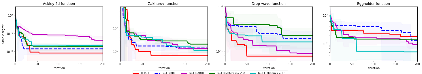
Figure 6: Simple regret of EGP-EI vs. GP-EI with a preselected kernel on Ackley-5d, Zakharov, DropWave and Eggholder function (from left to right). Dictionary has 4 kernels with distinct forms: RBF with(out) ARD and Matérn with $\nu=1.5,2.5$.

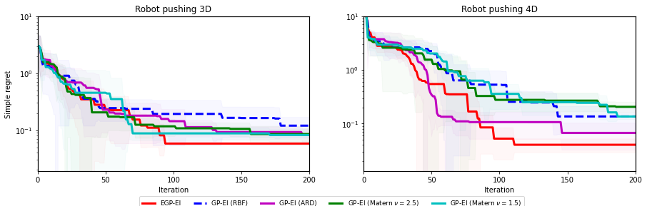
Figure 7: Simple regret of EGP-EI vs. GP-EI with a preselected kernel on Robot pushing 3D and Robot pushing 3D tasks (from left to right). Dictionary has 4 kernels with distinct forms: RBF with(out) ARD and Matérn with $\nu=1.5,2.5$.

Preliminary results for EGP-EI. Here, we couple the EGP surrogate with the EI acquisition rule [20], yielding the novel EGP-EI approach. In line with the proposed EGP-TS, one could first select a GP model by random sampling based on the weights ${\bf w}_{t}$, and then implement the EI acquisition function based on the chosen GP model. To benchmark the performance of this advocated EGP-EI, comparison has been made relative to GP-EI with a preselected kernel function. We use BoTorch to implement both EGP-EI and GP-EI with kernel hyperparameters updated every iteration and without RF approximation. As shown in Figs. 6-7, EGP-EI outperforms GP-EI in three out of the four synthetic functions and both of the robotic tasks – what demonstrates the benefits accompanied with the more expressive EGP model for the EI acquisition function. Rather than sampling a single GP from the EGP, future work includes investigation of the EI rule based on the GP mixture function model (cf. Remark 1).

References

• [1] Breast Cancer dataset. https://archive.ics.uci.edu/ml/datasets/breast+cancer.
• [2] Iris dataset. https://archive.ics.uci.edu/ml/datasets/iris.
• [3] MNIST dataset. http://yann.lecun.com/exdb/mnist/.
• [4] Transportation dataset. https://gisdata.mn.gov.
• [5] Wine dataset. https://archive.ics.uci.edu/ml/datasets/wine.
• [6] R. J. Adler. An introduction to continuity, extrema, and related topics for general Gaussian processes. IMS, 1990.
• [7] O. Chapelle and L. Li. An empirical evaluation of Thompson sampling. Proc. Adv. Neural Inf. Process. Syst., 24:2249–2257, 2011.
• [8] S. R. Chowdhury and A. Gopalan. On kernelized multi-armed bandits. pages 844–853, 2017.
• [9] A. Cully, J. Clune, D. Tarapore, and J.-B. Mouret. Robots that can adapt like animals. Nature, 521(7553):503–507, 2015.
• [10] T. Desautels, A. Krause, and J. W. Burdick. Parallelizing exploration-exploitation tradeoffs in Gaussian process bandit optimization. J. Mach. Learn. Res., 15:3873–3923, 2014.
• [11] J. Devlin, M.-W. Chang, K. Lee, and K. Toutanova. Bert: Pre-training of deep bidirectional transformers for language understanding. arXiv preprint arXiv:1810.04805, 2018.
• [12] D. Duvenaud, J. Lloyd, R. Grosse, J. Tenenbaum, and G. Zoubin. Structure discovery in nonparametric regression through compositional kernel search. Proc. Int. Conf. Mach. Learn., pages 1166–1174, 2013.
• [13] M. Feurer, B. Letham, and E. Bakshy. Scalable meta-learning for Bayesian optimization using ranking-weighted Gaussian process ensembles. In AutoML Workshop at ICML, volume 7, 2018.
• [14] P. I. Frazier. A tutorial on Bayesian optimization. arXiv preprint arXiv:1807.02811, 2018.
• [15] S. Ghosal and A. Roy. Posterior consistency of Gaussian process prior for nonparametric binary regression. The Annals of Statistics, 34(5):2413–2429, 2006.
• [16] S. Gopakumar, S. Gupta, S. Rana, V. Nguyen, and S. Venkatesh. Algorithmic assurance: An active approach to algorithmic testing using Bayesian optimisation. Proc. Adv. Neural Inf. Process. Syst., pages 5470–5478, 2018.
• [17] J. M. Hernández-Lobato, J. Requeima, E. O. Pyzer-Knapp, and A. Aspuru-Guzik. Parallel and distributed Thompson sampling for large-scale accelerated exploration of chemical space. Proc. Int. Conf. Mach. Learn., pages 1470–1479, 2017.
• [18] M. Hoffman, E. Brochu, N. de Freitas, et al. Portfolio allocation for bayesian optimization. Proc. Conf. Uncerntainty in Artif. Intel., pages 327–336, 2011.
• [19] J. Hong, B. Kveton, M. Zaheer, M. Ghavamzadeh, and C. Boutilier. Thompson sampling with a mixture prior. arXiv preprint arXiv:2106.05608, 2021.
• [20] D. R. Jones, M. Schonlau, and W. J. Welch. Efficient global optimization of expensive black-box functions. Journal of Global optimization, 13(4):455–492, 1998.
• [21] K. Kandasamy, A. Krishnamurthy, J. Schneider, and B. Póczos. Parallelised Bayesian optimisation via Thompson sampling. Proc. Int. Conf. Artif. Intel. and Stats., pages 133–142, 2018.
• [22] G. V. Karanikolas, Q. Lu, and G. B. Giannakis. Online unsupervised learning using ensemble Gaussian processes with random features. Proc. IEEE Int. Conf. Acoust., Speech, Sig. Process., pages 3190–3194, 2021.
• [23] H. Kim and Y. W. Teh. Scaling up the automatic statistician: Scalable structure discovery using Gaussian processes. Proc. Int. Conf. Artif. Intel. and Stats., pages 575–584, 2018.
• [24] K. Korovina, S. Xu, K. Kandasamy, W. Neiswanger, B. Poczos, J. Schneider, and E. Xing. Chembo: Bayesian optimization of small organic molecules with synthesizable recommendations. Proc. Int. Conf. Artif. Intel. and Stats., pages 3393–3403, 2020.
• [25] M. Lázaro-Gredilla, J. Quiñonero Candela, C. E. Rasmussen, and A. Figueiras-Vidal. Sparse spectrum Gaussian process regression. J. Mach. Learn. Res., 11(Jun):1865–1881, 2010.
• [26] Q. Lu and G. B. Giannakis. Gaussian process temporal-difference learning with scalability and worst-case performance guarantees. Proc. IEEE Int. Conf. Acoust., Speech, Sig. Process., pages 3485–3489, 2021.
• [27] Q. Lu and G. B. Giannakis. Robust and adaptive temporal-difference learning using an ensemble of Gaussian processes. arXiv preprint arXiv:2112.00882, 2021.
• [28] Q. Lu, G. Karanikolas, Y. Shen, and G. B. Giannakis. Ensemble Gaussian processes with spectral features for online interactive learning with scalability. Proc. Int. Conf. Artif. Intel. and Stats., pages 1910–1920, 2020.
• [29] Q. Lu, G. V. Karanikolas, and G. B. Giannakis. Incremental ensemble Gaussian processes. IEEE Trans. Pattern Anal. Mach. Intel., 2022.
• [30] G. Malkomes, C. Schaff, and R. Garnett. Bayesian optimization for automated model selection. Proc. Adv. Neural Inf. Process. Syst., 2016.
• [31] M. Mutnỳ and A. Krause. Efficient high dimensional Bayesian optimization with additivity and quadrature Fourier features. Proc. Adv. Neural Inf. Process. Syst., pages 9005–9016, 2019.
• [32] D. Nguyen, S. Gupta, S. Rana, A. Shilton, and S. Venkatesh. Bayesian optimization for categorical and category-specific continuous inputs. Proc. AAAI Conf. Artif. Intel., 34(04):5256–5263, 2020.
• [33] K. D. Polyzos, Q. Lu, and G. B. Giannakis. Ensemble gaussian processes for online learning over graphs with adaptivity and scalability. IEEE Trans. Sig. Process., 2021.
• [34] K. D. Polyzos, Q. Lu, and G. B. Giannakis. Graph-adaptive incremental learning using an ensemble of Gaussian process experts. Proc. IEEE Int. Conf. Acoust., Speech, Sig. Process., pages 5220–5224, 2021.
• [35] K. D. Polyzos, Q. Lu, and G. B. Giannakis. Online graph-guided inference using ensemble Gaussian processes of egonet features. Proc. Asilomar Conf. Sig., Syst., Comput., pages 182–186, 2021.
• [36] K. D. Polyzos, Q. Lu, A. Sadeghi, and G. B. Giannakis. On-policy reinforcement learning via ensemble Gaussian processes with application to resource allocation. Proc. Asilomar Conf. Sig., Syst., Comput., pages 1018–1022, 2021.
• [37] A. Rahimi and B. Recht. Random features for large-scale kernel machines. Proc. Adv. Neural Inf. Process. Syst., pages 1177–1184, 2008.
• [38] C. E. Rasmussen and C. K. Williams. Gaussian processes for machine learning. MIT press Cambridge, MA, 2006.
• [39] W. Rudin. Principles of Mathematical Analysis, volume 3. McGraw-hill New York, 1964.
• [40] D. Russo and B. Van Roy. Learning to optimize via posterior sampling. Mathematics of Operations Research, 39(4):1221–1243, 2014.
• [41] B. Shahriari, K. Swersky, Z. Wang, R. P. Adams, and N. De Freitas. Taking the human out of the loop: A review of Bayesian optimization. Proc. IEEE, 104(1):148–175, 2015.
• [42] B. Shahriari, Z. Wang, M. W. Hoffman, A. Bouchard-Côté, and N. de Freitas. An entropy search portfolio for Bayesian optimization. arXiv preprint arXiv:1406.4625, 2014.
• [43] J. Snoek, H. Larochelle, and R. P. Adams. Practical Bayesian optimization of machine learning algorithms. Proc. Adv. Neural Inf. Process. Syst., 25, 2012.
• [44] N. Srinivas, A. Krause, S. M. Kakade, and M. W. Seeger. Information-theoretic regret bounds for Gaussian process optimization in the bandit setting. IEEE Trans. Inf. Theory, 58(5):3250–3265, 2012.
• [45] T. Teng, J. Chen, Y. Zhang, and B. K. H. Low. Scalable variational Bayesian kernel selection for sparse Gaussian process regression. Proc. AAAI Conf. Artif. Intel., 34(04):5997–6004, 2020.
• [46] W. R. Thompson. On the likelihood that one unknown probability exceeds another in view of the evidence of two samples. Biometrika, 25(3/4):285–294, 1933.
• [47] R. Turner, D. Eriksson, M. McCourt, J. Kiili, E. Laaksonen, Z. Xu, and I. Guyon. Bayesian optimization is superior to random search for machine learning hyperparameter tuning: Analysis of the black-box optimization challenge 2020. arXiv preprint arXiv:2104.10201, 2021.
• [48] S. Vakili, V. Picheny, and A. Artemev. Scalable Thompson sampling using sparse Gaussian process models. Proc. Adv. Neural Inf. Process. Syst., 2021.
• [49] J. Wang, S. C. Clark, E. Liu, and P. I. Frazier. Parallel Bayesian global optimization of expensive functions. arXiv preprint arXiv:1602.05149, 2016.
• [50] Z. Wang, C. Gehring, P. Kohli, and S. Jegelka. Batched large-scale Bayesian optimization in high-dimensional spaces. Proc. Int. Conf. Artif. Intel. and Stats., pages 745–754, 2018.
• [51] Z. Wang and S. Jegelka. Max-value entropy search for efficient Bayesian optimization. Proc. Int. Conf. Mach. Learn., pages 3627–3635, 2017.
• [52] J. Wilson, V. Borovitskiy, A. Terenin, P. Mostowsky, and M. Deisenroth. Efficiently sampling functions from Gaussian process posteriors. Proc. Int. Conf. Mach. Learn., pages 10292–10302, 2020.