Abstract

Use of dedicated computers in spin glass simulations allows one to equilibrate very large samples (of size as large as $L=32$) and to carry out computer experiments that can be compared to (and analyzed in combination with) laboratory experiments on spin-glass samples. In the absence of a magnetic field, the most economic conclusion of the combined analysis of equilibrium and non-equilibrium simulations is that an RSB spin glass phase is present in three spatial dimensions. However, in the presence of a field, the lower critical dimension for the de Almeida-Thouless transition seems to be larger than three.

Chapter 0 Numerical Simulations and Replica Symmetry Breaking

1 Introduction

Equilibrium numerical simulations have been an important tool used by the scientific community to decide the theoretical controversy regarding the main features of the spin glass phase (SG) at low temperatures $T<T_{\mathrm{c}}$ ($T_{\mathrm{c}}$ is the critical temperature). On one side of this polemic, Parisi’s solution of the SG in the mean field approximation [1] has evolved into the replica symmetry breaking (RSB) theory [2] according to which the spin-glass phase has many pure states. It can be regarded as as a critical phase for all $T<T_{\mathrm{c}}$ in which the surfaces of the magnetic domains are space filling. On the other hand, according to the droplet theory [3, 4, 5, 6] there are only two pure states (in zero field) and the surfaces of magnetic domains (droplets) have a fractal dimension less than the space dimension $D$. It corresponds to the Migdal-Kadanoff approximation [7]. There is also an intermediate picture [8, 9] called TNT for “trivial-non trivial”.

However, the emphasis has changed somewhat in recent times. Recent numerical work has mostly focused in out-of-equilibrium simulations (a choice partly motivated by the fact that experimental work in spin glasses is carried out under non-equilibrium conditions). The so-called static-dynamic equivalence allows one to quantitatively relate quantities computed in equilibrium with out-of-equilibrium analogues (see e.g. Ref. [10, 11, 12, 13, 14, 15, 16]). Dedicated computers, see Sec. 2, have had an important role in this shift of focus that has allowed for a new level of collaboration between simulations and experiments in spin-glass physics. Indeed, it has become possible nowadays to subject experimental and numerical data to a parallel analysis (see Refs. [17, 18, 19] and Sec. 5 in this chapter). From this new perspective, the situation about the droplet/RSB polemic takes a different light depending on the presence (or absence) of an external magnetic field:

• In the absence of a magnetic field, the latest results, both in equilibrium (see Sec. 3) and out-of-equilibrium (Sec. 5), find an RSB phase for $T<T_{\mathrm{c}}$ and space dimension $D\!=\!3$. The droplet scenario still remains as a logical possibility, but only if one is willing to accept that current simulations and experiments are entirely carried out far from the asymptotic regime.

• In the presence of a magnetic field, however, finding a spin-glass phase in $D\!=\!3$ has turned out to be extremely difficult. There is, however, evidence for a spin glass phase in a field in large $D$, see Sec. 4.

Due to space limitations, we shall restrict ourselves to the case of Ising spins ($S_{\boldsymbol{x}}=\pm 1$), even though Heisenberg and XY spin glass models are also interesting. Their transition temperature is surprisingly low, the asymptotic scaling behavior has probably not been obtained accurately, and there is controversy as to whether there is a separate transition involving chiralities, with Kawamura arguing in favor of a separate transition [20, 21, 22, 23, 24], and other authors disagreeing [25, 26, 27]. Nevertheless, universality arguments suggest that the unavoidable residual anisotropies in the spin interactions cause the distinction between Ising and Heisenberg spin glasses to be asymptotically irrelevant [28, 29]. The question is not yet clear. On the one hand, maybe due to the difficulties in probing the asymptotic scaling regime, critical exponents do not seem to match. For instance, the exponent $\gamma$ for the non-linear susceptibility is approximately $5.5$ from simulations for the Ising spin-glass universality class [30], while experiments on Heisenberg spin glasses get lower values around 2 and 3 [31]. On the other hand, the quantitative agreement in the non-equilibrium dynamics in the spin glass phase between experiments in CuMn samples and Ising-Edwards-Anderson simulations, see Refs. [17, 18, 19] and Sec. 5, seems to support the choice of modeling spin glasses with an Ising Hamiltonian.

The remaining part of this chapter is organized as follows. We recall the standard model of spin-glasses in Sec. 1, define the main observables considered in equilibrium simulations in Sec. 2, and review finite-size scaling methods in Sec. 3. The need for dedicated computers is explained in Sec. 2. Important results obtained in equilibrium simulations in the absence of a magnetic field are recalled in Sec. 3. Equilibrium simulations in a field are reviewed in Sec. 4. Next, out-of-equilibrium simulations are reviewed in Sec. 5, and finally, our conclusions are summarized in Sec. 6.

1 The Edwards-Anderson Model and its gauge symmetry

We shall be considering two geometries, namely (hyper) cubic lattices in $D$-dimensions and $1D$ models with long-range interactions. In the cubic geometry, the spins lie on the nodes of a (hyper)cubic lattice, whose linear size is denoted by $L$, so the number of spins is $N=L^{D}$. Periodic boundary conditions are usually taken and interactions are typically restricted to lattice nearest-neighbors. The models with long-range interactions are in one dimension and the strength of the interactions falls off as a power of the distance between the spins. Varying this power is argued to be equivalent (at least roughly) to varying the dimension of the short-range model.

For both geometries, we consider the Edwards-Anderson (EA) Hamiltonian:

$$\mathcal{H}=-\sum_{\langle\boldsymbol{x},\boldsymbol{y}\rangle}J_{\boldsymbol{x}\boldsymbol{y}}S_{\boldsymbol{x}}S_{\boldsymbol{y}}-\sum_{\boldsymbol{x}}h_{\boldsymbol{x}}S_{\boldsymbol{x}},$$ (1)

where $\langle\boldsymbol{x},\boldsymbol{y}\rangle$ indicates that the sum is taken over all pairs of interacting spins (e.g. nearest-neighbors for the typical cubic geometry). It would be natural to use a uniform, external magnetic field $h_{\boldsymbol{x}}=h$, but the gauge symmetry (see below) makes it advisable to retain a site-dependence for the magnetic fields $h_{\boldsymbol{x}}$. Spin glass models have quenched disorder (see e.g. Ref. [32]) in which the coupling constants $J_{\boldsymbol{x}\boldsymbol{y}}$ (and sometimes also the magnetic fields $h_{\boldsymbol{x}}$) are randomly extracted from a probability distribution and held fixed once and for all. We call a particular realization of the $\{J_{\boldsymbol{x}\boldsymbol{y}},h_{\boldsymbol{x}}\}$ a sample. Thermal averages, denoted by $\langle\ldots\rangle$, are first computed for every sample. The subsequent average over samples of the thermal mean-values is denoted by $[\langle\ldots\rangle]$.

The couplings in Eq. (1) are independent, identically distributed random variables. The most popular choices for the probability distributions in a cubic geometry are the bimodal distribution (in which $J_{\boldsymbol{x}\boldsymbol{y}}$ is $\pm 1$ with $50\%$ probability) and a Gaussian distribution with zero mean and unit variance. In the case of the long-range geometry, one usually takes a Gaussian distribution.

The crucial role of the $Z_{2}$ Gauge symmetry of the Hamiltonian (1) was soon realized [33]. If one chooses $\epsilon_{\boldsymbol{x}}=\pm 1$ randomly at every lattice site $\boldsymbol{x}$, the energy remains invariant under the transformation

$$S_{\boldsymbol{x}}\rightarrow\epsilon_{\boldsymbol{x}}S_{\boldsymbol{x}}\,,\quad J_{\boldsymbol{x}\boldsymbol{y}}\rightarrow\epsilon_{\boldsymbol{x}}J_{\boldsymbol{x}\boldsymbol{y}}\epsilon_{\boldsymbol{y}}\,,\quad h_{\boldsymbol{x}}\rightarrow\epsilon_{\boldsymbol{x}}h_{\boldsymbol{x}}\,.$$ (2)

For all the standard choices of coupling distributions, one finds that the original choice $\{J_{\boldsymbol{x}\boldsymbol{y}},h_{\boldsymbol{x}}\}$ and its gauge-transformed values $\{\epsilon_{\boldsymbol{x}}J_{\boldsymbol{x}\boldsymbol{y}}\epsilon_{\boldsymbol{y}}\,\epsilon_{\boldsymbol{x}}h_{\boldsymbol{x}}\}$ occur with the same probability. Therefore, the sample-average $[\langle\ldots\rangle]$ effectively averages over all possible choices for the gauge parameters $\epsilon_{\boldsymbol{x}}=\pm 1$. All quantities that we focus on are invariant under the gauge transformation (2), see Secs. 2, 1.

2 Observables (equilibrium)

A key quantity in our discussion will be the total overlap per spin defined by:

$$q\equiv q_{1,2}=\frac{1}{N}\sum_{\boldsymbol{x}}S_{\boldsymbol{x}}^{(1)}S_{\boldsymbol{x}}^{(2)}\,,$$ (3)

where $S^{(1)}$ and $S^{(2)}$ are two real replicas of the system with the same disorder. Its associated probability density function (pdf) averaged over the disorder can be written as

$$P(q)=\left[\left\langle\delta\left(q-\frac{1}{N}\sum_{\boldsymbol{x}}S_{\boldsymbol{x}}^{(1)}S_{\boldsymbol{x}}^{(2)}\right)\right\rangle\right]\,.$$ (4)

It will also be useful to define the link overlap by

$$Q_{\mathrm{link}}=\frac{1}{N_{\text{link}}}\sum_{\langle\boldsymbol{x},\boldsymbol{y}\rangle}S^{(1)}_{\boldsymbol{x}}S^{(1)}_{\boldsymbol{y}}S^{(2)}_{\boldsymbol{x}}S^{(2)}_{\boldsymbol{y}}\,,$$ (5)

where the sum extends over all pairs of interacting lattice-sites (also known as links), whose number is ${N_{\text{link}}}$. In a $D$-dimensional cubic lattice with periodic boundary conditions ${N_{\text{link}}}=DN$, but for a long-range model ${N_{\text{link}}}$ may be as large as $N(N-1)/2$. In mean field theory the link overlap is trivially related to the spin overlap by $Q_{\mathrm{link}}=q^{2}$.

Both $q$ and $Q_{\text{link}}$ are adequate for a mean-field treatment, but to go beyond this limit also we need to consider the crucial role of fluctuations, characterized by correlation functions. In the presence of a magnetic field, where individual spins have a non-zero average, several different correlation functions can be defined [34, 35]. Specializing here only to the most divergent correlations [36, 37], we define the “replicon” propagator in real and Fourier space by

$$G(\boldsymbol{r})=\frac{1}{N}\sum_{{\boldsymbol{x}}}\left[\,\left(\,\langle S_{\boldsymbol{x}}S_{{\boldsymbol{x}}+{\boldsymbol{r}}}\rangle-\langle S_{\boldsymbol{x}}\rangle\langle S_{{\boldsymbol{x}}+{\boldsymbol{r}}}\rangle\,\right)^{2}\,\right]\,,\quad\hat{G}(\boldsymbol{k})=\sum_{\boldsymbol{r}}\ \mathrm{e}^{-\mathrm{i}{\boldsymbol{k}}\cdot{\boldsymbol{r}}}\,G(\boldsymbol{r})\,.$$ (6)

In particular, the spin-glass susceptibility is

$$\chi_{SG}\equiv\hat{G}\big{(}{\boldsymbol{k}}=(0,0,\ldots,0)\big{)}=\frac{1}{N}\sum_{{\boldsymbol{x}},{\boldsymbol{y}}}\left[\,\left(\,\langle S_{\boldsymbol{x}}S_{\boldsymbol{y}}\rangle-\langle S_{\boldsymbol{x}}\rangle\langle S_{\boldsymbol{y}}\rangle\,\right)^{2}\,\right]\,.$$ (7)

In the absence of a field, $\langle S_{\boldsymbol{x}}\rangle=0$ for all sites ${\boldsymbol{x}}$ and Eq. (7) simplifies to $\chi_{SG}=N\big{[}\langle q^{2}\rangle\big{]}$.

A quantity related to $\chi_{SG}$ is the second-moment correlation length (see e.g. [38]) that in a (hyper)cubic lattice with periodic boundary conditions is

$$\xi_{2}=\frac{1}{2\sin(\pi/L)}\sqrt{\frac{\chi_{SG}}{\hat{G}({\boldsymbol{k}}_{1})}-1}\,,$$ (8)

where ${\boldsymbol{k}_{1}}$ is the minimal non-vanishing wavevector allowed by the boundary conditions (namely, ${\boldsymbol{k}}_{1}=(2\pi/L,0,0,\ldots,0)$ and permutations). Interestingly, $\xi_{2}$ was instrumental in showing that there is a second order spin glass phase transition in zero field in space dimension $D\!=\!3$ [39, 40]. A different definition of the correlation length, more appropriate for out-of-equilibrium simulations, will be discussed in Sec. 1.

Let us conclude this paragraph by recalling a most important quantity, namely the Edwards-Anderson order parameter ($q_{\mathrm{EA}}$), which is the maximum overlap. For mean-field models (such as the Sherrington-Kirkpatrick (SK) model), $q_{\mathrm{EA}}$ is given by

$$q_{\mathrm{EA}}=\sum_{\boldsymbol{x}}\big{[}\langle S_{\boldsymbol{x}}\rangle_{\alpha}^{2}\big{]}\,.$$ (9)

where $\langle(\cdots)\rangle_{\alpha}$ is the average constrained to the state $\alpha$ and is independent of the choice of the state. Unfortunately, the definition of a state beyond the mean-field approximation is quite subtle (see the chapter by Newman, Read and Stein in this volume).

3 Finite Size Scaling

The theory of finite-size scaling, see e.g. [38], explains how critical divergencies are rounded in a finite-system of linear size $L$. Let $T_{\text{c}}(h)$ be the critical temperature, in which we have allowed a dependency on the magnetic field $h$, and let $O$ be a quantity diverging in the thermodynamic limit as $\big{[}\langle O\rangle\big{]}\propto 1/(T-T_{\text{c}}(h))^{x_{o}}$ (we refer only to the dominant divergence, there might be subleading terms). If the space dimension $D$ is smaller than the upper critical dimension $D_{u}$ (the dimension above which the mean-field approximation gives exact values for critical exponents) then, according to finite-size scaling,

$$\big{[}\langle O\rangle\big{]}(L,T)=L^{x_{o}/\nu}f_{O}(L^{1/\nu}t\bigr{)}+\ldots,\quad t=\frac{T-T_{\text{c}}(h)}{T_{\text{c}}(h)}\,,$$ (10)

where $\nu$ is the thermal critical exponent and the dots stand for subleading scaling corrections.

Of particular importance in this context are dimensionless quantities such as the second-moment correlation length $\xi_{2}$, defined in Eq. (8), in units of the system-size

$$\xi_{2}/L=f_{\xi}\bigl{(}L^{1/\nu}t\bigr{)}+\ldots\,.$$ (11)

Dimensionless quantities are extremely useful to locate the critical point see, for instance, Ref. [40]. An example of this use of Eq. (11) is explained in Sec. 4 and Fig. 5.

Some authors, working with $1D$ models with long-range interactions, have found that, in the presence of an external magnetic field, the propagator behaves anomalously, but only for the $\boldsymbol{k}=0$ mode [41]. This observation suggest trading $\xi_{2}/L$ for another universal, renormalization-group invariant quantity named $R_{12}$ [42], defined by

$$R_{12}=\frac{\hat{G}(\boldsymbol{k}_{1})}{\hat{G}(\boldsymbol{k}_{2})},$$ (12)

where ${\boldsymbol{k}_{1}}$ and ${\boldsymbol{k}_{2}}$ are the smallest non-zero momenta compatible with the periodic boundary conditions. For example, for $D\!=\!4$, $\boldsymbol{k}_{1}\!=\!(2\pi/L,0,0,0)$ and $\boldsymbol{k}_{2}\!=\!(2\pi/L,\pm 2\pi/L,0,0)$ (and permutations). The generalization to other space dimensions is trivial.

2 Why it is so difficult to simulate spin glasses? The role of dedicated computers.

Numerical simulation of spin glasses in equilibrium entails two major difficulties:

1. The variability between different samples is quite significant (see, for instance, sec. 3), which means that one needs to simulate a large number of samples in order to obtain an accurate sample average.

2. The simulation time need to equilibrate each sample is very significant. This is to be expected at zero temperature, because finding the ground gtate is an NP-complete problem [43]. The problem remains difficult at finite temperatures. The most efficient Monte Carlo algorithm for spin glasses seems to be parallel tempering[44, 45], also called “replica exchange Monte Carlo”. Unfortunately there is no known, highly-efficient cluster algorithm of general applicability to spin glasses which corresponds to Swendsen and Wang’s [46] cluster algorithm for unfrustrated systems. In separate work, Swendsen and Wang [47] developed a cluster-replica approach to spin glasses which works well in two dimensions [48]. In higher dimensions, though, this approach effectively becomes equivalent to parallel tempering. A cluster, replica algorithm for $D\!=\!2$ spin glasses has also been developed by Houdayer [49]. Since $T_{c}=0$ for two-dimensional spin glasses, so there is no low-temperature phase, the most efficient algorithm for the spin glass state below $T_{c}$ seems to be parallel tempering, as noted above. Even with the help of parallel tempering, some samples need an inordinately large equilibration time [25]. The underlying physical mechanism that hampers equilibration, even when using parallel tempering, seems to be temperature chaos [50, 51].

For out-equilibrium simulations, one uses very large samples to ensure that the slowly growing, time-dependent coherence length $\xi(t)$ is much less than the system size $L$. One then needs fewer samples than for equilibrium simulations because one can think of a macroscopic sample as being composed of $(L/\xi(t))^{D}$ equilibrated regions which are more or less independent of each other, so one large sample effectively averages over $(L/\xi(t))^{D}$ “samples” of size $L_{\text{eff}}\approx\xi(t)$. If one could simulate a truly macroscopic system then only one sample would be needed. This is, of course, the experimental situation.

Another difficulty in out-of-equilibrium simulations is that one has to mimic natural dynamics using, for instance, the Metropolis algorithm. One is not allowed to use accelerated dynamics like parallel tempering. Unfortunately, natural dynamics is very slow at and below $T_{\mathrm{c}}$ (see e.g. Fig. 11). Hence, it is clear that one needs to carry out very long simulations in order to reach reasonably large values of $\xi(t)$. This topic is further elaborated in Sec. 5.

Given these difficulties, a possible way forward is to build computers specifically designed for spin-glass simulations. Several such computers have been built over the years, such as the Ogielski machine [53], SUE [54], and the Janus supercomputers [55, 56]. The Janus II is currently the most powerful computer for spin glass simulations.

3 Equilibrium numerical studies of the overlap

RSB makes many predictions regarding the order parameter in spin glasses. In this section we will focus on a small number of them: (i) its density probability function $P(q)$, (ii) overlap equivalence, i.e. all possible definitions of an overlap in the model encode the same physics and (iii) stochastic stability (which is used to show the Guerra’s relations) and ultrametricity.

1 Structure of the Equilibrium $P(q)$

\begin{overpic}[width=361.34999pt,trim=30.11249pt 140.525pt 30.11249pt 155.58124pt,clip]{FIGURES/figura_Pq.pdf} \put(28.0,38.0){{\bf(a)}} \put(80.0,40.0){{\bf(b)}} \put(80.0,21.0){{\bf(c)}} \end{overpic}

Figure 1: (a) Overlap density distribution function $P(q)$, see Eq. (4), as computed for the $3D$ EA model with binary couplings at $T=0.703\!\approx\!0.64T_{\mathrm{c}}$ for different lattice sizes $L$. (b) is $P(q=0)$ and (c) is $P(q=0)/T$ versus temperature $T$, as computed in $3D$ for several system sizes. We observe an envelope curve with a linear behavior, as expected from RSB. Figure adapted from[57].

One manifestation of the infinite number of pure states predicted by RSB theory is a non trivial pdf of the order parameter, $P(q)$, see Fig. 1(a). In contrast, the droplet model predicts a trivial $P(q)$ in the thermodynamic limit, in the sense that it consists, for $h=0$, of two Dirac-delta functions at $q\!=\!\pm q_{\mathrm{EA}}$, where $q_{\mathrm{EA}}$ is the Edwards-Anderson overlap. Instead, in RSB, $P(q)$ has, in addition to these two delta functions, a continuous function in between which is non-zero in the thermodynamic limit. In the droplet picture the continuous part of the distribution vanishes slowly with linear system size $L$ like $L^{-\theta_{S}}$ where $\theta_{S}$ is a stiffness exponent whose value is around $0.24$ [58] for $D\!=\!3$.

Over the years there have been many studies [59, 60, 61, 62, 63, 64, 57, 65] of the weight of $P(q)$ around $q\!=\!0$ and these consistently find a value independent, or nearly independent, of size, in agreement with RSB theory.

We show some recent results in $3D$ [57] for $P(q)$, Fig 4(a), $P(0)$, Fig 4(b), and $P(0)/T$, Fig 4(c), as a function of the temperature deep in the spin glass phase. We recall that $T_{c}=1.1019(29)$[30]. This data supports the RSB predictions that $P(0)$ is independent of $L$, and is proportional to $T$ at low $T$. A different analysis of the $P(q)$ behavior comes to the same conclusions [65]. The behavior of $P(q\!=\!0)$ could be modified by the presence of interfaces, so it was proposed to compute $P(q)$ in small boxes in order to avoid their effects. This analysis was performed in Ref. [66], which found the same behavior as that obtained from the overlap computed over the whole lattice.

2 Overlap Equivalence

Overlap equivalence states that all possible definitions of new overlaps in a spin glasses must be a function of the overlap $q$. Equivalently, we can classify a pair of replicas using their overlap and argue that no finer classification is possible (separability). This implies that fluctuations of all reasonable definitions of the overlap will vanish if we work in a $q$-fixed ensemble.

The variance of a $q$-conditioned observable $O$ is defined by

$$\mathrm{Var}(O|q=c)=\mathrm{E}(O^{2}|q=c)-\mathrm{E}(O|q=c)^{2}\,.$$ (13)

where the symbol $\mathrm{E}(\cdot)$ denotes (i) the average in a given sample over the configurations which satisfy the constraint ($q\!=\!c$), and then (ii) the average over disorder.

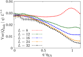
Figure 2: Plot of the conditional variance at fixed $q$ of $Q_{\mathrm{link}}$, see Eq. (13), rescaled by appropriate powers of $L$ in $3D$ at $T=0.703$ (we chose exponents that provided a good scaling at $q\!=\!0$). The abscissa corresponds to $q$ in units of $q_{\mathrm{EA}}(L,T=0.703)$. Figure taken from [57].

In this subsection we address the behavior of $\mathrm{Var}(Q_{\mathrm{link}}|q)$. RSB predicts that this conditioned variance should go to zero in the limit of large lattices, due to the existence of a relation between $Q_{\mathrm{link}}$ and $q$. In the droplet model the only possible value of $q$ is $q_{\mathrm{EA}}$, so $Q_{\mathrm{link}}$ will be defined only for this value of the overlap (in the infinite volume limit). Therefore, the droplet model predicts as well a vanishing conditioned variance.

Indeed, Fig. 2 shows that this conditioned variance goes to zero in the limit of large $L$[57]. Moreover, Ref. [67] reaches the same conclusion from a different analysis. The good scaling of the conditioned variance of $Q_{\mathrm{link}}$ near $q\!=\!0$ extends to $q_{EA}$ for the larger lattices ($L\!=\!24$ and $L\!=\!32$). This scaling supports RSB and not droplet, because in the droplet picture it would be natural to expect completely different finite size effects for $q\!=\!q_{\mathrm{EA}}$ and for $q<q_{\mathrm{EA}}$ (and in particular for $q\!=\!0$).

Another interesting quantity is $\mathrm{d}\mathrm{E}(Q_{\mathrm{link}}|q)/\mathrm{d}q^{2}$. In the droplet model, at variance with the RSB picture, this derivative should be zero. Numerically, the derivative is nonzero, although its size decreases with $L$. Therefore, the analysis based on this observable is not conclusive [57]. Nevertheless the results of Ref. [67], present numerical evidences that $\mathrm{E}(Q_{\mathrm{link}}|q^{2})$ is an increasing one-to-one function of $q^{2}$ in the thermodynamic limit. This fact, when combined with a vanishing conditioned variance of $Q_{\mathrm{link}}$, rules out the TNT description of the spin-glass phase.

3 Stochastic Stability

Stochastic stability has been proved in the SK model by Guerra [68, 69] and by Aizenman and Contucci [70]. In this section we present numerical evidence supporting stochastic stability in finite dimensional models, which, in turn, provides evidence that RSB applies in those systems.

Using stochastic stability is possible to write the following relation,

$$R_{\mathrm{link}}=\frac{\big{[}\langle Q_{\mathrm{link}}^{2}\rangle-\langle Q_{\mathrm{link}}\rangle^{2}\big{]}}{\big{[}\langle Q_{\mathrm{link}}^{2}\rangle\big{]}\ -\ \big{[}\langle Q_{\mathrm{link}}\rangle\big{]}^{2}}=\frac{2}{3}\qquad(\mathrm{RSB\ },L\to\infty,T<T_{c})\,.$$ (14)

Note the difference in the placement of the square in the subtracted terms in the numerator and denominator. In the droplet or TNT pictures both the numerator and denominator vanish in the thermodynamic limit.

Another analogous observable with the same RSB behavior is $R_{q^{2}}$ (using the mean-field correspondence $Q_{\mathrm{link}}\rightarrow q^{2}$):

$$R_{q^{2}}=\frac{\big{[}\langle q^{4}\rangle\ -\ \langle q^{2}\rangle^{2}\big{]}}{\big{[}\langle q^{4}\rangle\big{]}\ -\ \big{[}\langle q^{2}\rangle\big{]}^{2}}=\frac{2}{3}\qquad(\mathrm{RSB\ },L\to\infty,T<T_{c})\,.$$ (15)

\begin{overpic}[height=433.62pt,angle={270}]{FIGURES/estabilidad_estocastica} \put(55.0,60.0){{\bf(a)}} \end{overpic}

\begin{overpic}[height=433.62pt,angle={270}]{FIGURES/estabilidad_estocastica_q2} \put(55.0,60.0){{\bf(b)}} \end{overpic}

Figure 3: The ratios $R_{\mathrm{link}}$, Eq. (14), (a) and $R_{q^{2}}$, Eq. (15), (b) versus $T$ for the different system sizes in $3D$. Stochastic stability implies that, in an RSB system below $T_{\mathrm{c}}$, $R^{\mathrm{link}}=R_{\mathrm{q^{2}}}=2/3$ in the large-$L$ limit. Recall that $T_{\mathrm{c}}\approx 1.1$. Figure taken from [57].

In Fig. 3 we show the behavior of $R_{\mathrm{link}}$ and $R_{q^{2}}$ as a function of temperature in $3D$ for different lattice sizes. The convergence of both observables to the mean field limit, 2/3, is very good below the critical temperature. For additional analysis, see Ref. [67].

Finally, we briefly discuss the issue of ultrametricity. It is possible to show that overlap equivalence and stochastic stability imply ultrametricity [71]. In addition, using some of the Guerra’s relations [68, 69] and assuming the existence of ultrametricity in finite space dimension $D$, one finds that ultrametricity at finite $D$ should have the same properties that one finds for $D\!=\!\infty$ (i.e. a quarter of the triangles are equilateral, otherwise they are isosceles) [72]. Furthermore, Panchenko has shown that ultrametricity follows from stochastic stability without additional assumptions [73]. Hence, the results already presented in this section indicate that ultrametricity should exist in three-dimensions with the same properties as in mean field theory. However, direct detection of ultrametricity in 3$D$ spin glasses remains elusive [74, 75].

4 Results in a magnetic field

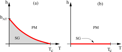
Figure 4: Schematic representation of the magnetic-field, temperature, ($h,T)$, phase diagram for a spin-glass. According to RSB theory, the phase diagram depends strongly on the space dimension. (a) If the space dimension is larger than the lower critical dimension (in a field) $D>D_{\mathrm{\ell}}^{h}$, there is a spin-glass phase (SG) for $T\!<\!T_{\mathrm{c}}(h)$. For $T>T_{\mathrm{c}}(h)$ the system is in the paramagnetic phase (PM). The critical line separating both phases, $T\!=\!T_{\mathrm{c}}(h)$, is called the deAlmeida-Thouless (dAT) line [34]. The value of the critical field at $T\!=\!0$ is called $h_{\mathrm{AT}}$. (b) Instead, for spatial dimension $D\!<\!D_{\mathrm{\ell}}^{h}$, a spin-glass phase exists only for $h\!=\!0$. According to the droplet picture, figure (b) applies in all dimensions, which corresponds to $D_{\mathrm{\ell}}^{h}\!=\!\infty$.

One of the most striking predictions of the RSB solution of the SK model [76] is a line of transitions in a magnetic field terminating in the zero field transition point, $T_{\mathrm{c}}$, see figH:dAT(a). This was first found by de Almeida and Thouless [34] and so is known as the dAT line. Below the dAT line, the SK model is described by the RSB solution of Parisi [77, 78, 79], while above the dAT line the replica symmetric solution is valid. According to RSB theory, there is also a dAT line in short-range models. If there is no dAT line, then there is simply a line of transitions along the zero field axis, terminating at $T_{\mathrm{c}}$, as shown in figH:dAT(b). This is the prediction of the droplet theory.

While the zero field transition has a spontaneously broken symmetry, as usual, the transition in a field on the dAT line is unusual in having no broken symmetry, since spin-inversion symmetry is already broken by the magnetic field. While the dAT transition definitely occurs in the SK model, there is controversy as to whether it also occurs in models which do not have infinite-range interactions. According to RSB theory there is a dAT line in short-range models, whereas according to the droplet theory the dAT line is an artefact of the infinite-range nature of the SK model and does not occur in short-range models in any dimension.

In critical phenomena, we are familiar with the fact that fluctuations destroy a transition in dimension $D$ below a “lower critical dimension”, $D_{\mathrm{\ell}}$, where $D_{\mathrm{\ell}}\!=\!1$ for the Ising ferromagnet (see e.g. Ref. [80]), and $D_{\mathrm{\ell}}\!\approx\!2.5$ for the Ising spin-glass [58, 81, 82]. What about the spin glass in a magnetic field? The gauge symmetry in Eq. (2) implies that even a uniform magnetic field in a spin glass is effectively a random-field as far as the spin glass ordering is concerned. This observation reminds us immediately of the random field Ising model (RFIM, see e.g. [83]).

When random-fields are switched on, they energetically favor spin configurations which are completely unrelated to the ferromagnetic (or spin-glass) ordered configurations that one finds in the absence of a field. The outcome of this competition crucially depends on the space dimension. If $D\!>\!D_{\mathrm{\ell}}^{h}$, the low-temperature ordered phase survives in the presence of small random-fields, while if $D\!<\!D_{\mathrm{\ell}}^{h}$, the slightest random-field destabilizes the ordered phase, see figH:dAT(b). Clearly $D_{\mathrm{\ell}}^{h}\geq D_{\mathrm{\ell}}$ and indeed for the RFIM, $D_{\mathrm{\ell}}^{h}\!=\!2$, which is greater than $D_{\mathrm{\ell}}\!=\!1$. Unfortunately, a consensus has not yet emerged about the value of $D_{\mathrm{\ell}}^{h}$ for the spin glass. Here will discuss some numerical attempts to determine it.

de Almeida and Thouless [34] computed the stability of the replica symmetric solution of the SK model, finding that an eigenvalue went negative (indicating instability) below the dAT line. Fortunately, this instability can be located in simulations because the unstable (“replicon”) eigenvalue is the inverse of the spin glass susceptibility $\chi_{SG}$ in the presence of a magnetic field, recall Eq. (7).

Hence the goal is to locate a divergence in $\chi_{SG}$. Of course no divergence occurs in the finite systems which are simulated, so we need to locate the dAT line by finite-size scaling (FSS), recall Sect. 3. This is most straightforward using a dimensionless quantity such as $\xi_{2}/L$ where $\xi_{2}$ is the correlation length of a finite system (second-moment correlation length), defined in Eq. (8). Now we recall Eq. (11), which indicates that the data for $\xi_{2}/L$ for different sizes intersects at the transition and splays out again on the low temperature side. We therefore look for intersections in the data.

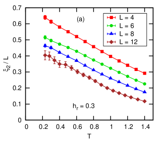
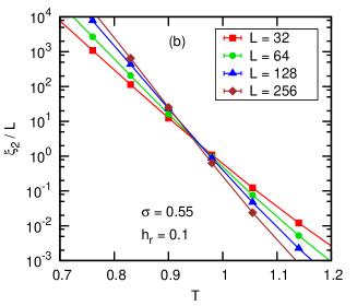
Figure 5: (a): Temperature dependence of the second-moment correlation length in units of the lattice size, $\xi_{2}/L$, as computed in spatial dimension $D\!=\!3$ for cubic samples of linear size $L$. The computation was carried out for Gaussian-distributed couplings and random fields, with zero mean and standard deviations $\sigma_{J}\!=\!1$ (this actually sets the energy units) and $\sigma_{h}\!=\!h_{\mathrm{r}}\!=\!0.3$. The lack of intersections down to the lowest temperature $T\!=\!0.23$ suggests that $D\!=\!3$ lies below the lower-critical dimension in a field, recall figH:dAT. The figure is adapted from Ref. [84]. (b): Second moment correlation length for a model with long-range power-law interactions for parameters corresponding to a short-range model in dimension $D$ greater than 6, which is the “upper critical dimension” for the spin glass in zero field. The intersections suggest that there is a dAT line in this region. Adapted from Ref. [85].

Early studies did not find a spin glass transition in a field in $D\!=\!3$ using standard FSS methods [84, 86], see figH:xiLoverLYK2004(a). It is difficult to directly simulate spin glasses in high dimensions, because the number of sites $N\!=\!L^{D}$ increases so fast with linear size $L$, that one can not equilibrate enough values of $L$ to perform FSS. Instead, it has been proposed to study models in 1$D$ with long-range interactions which fall off as a power $\sigma$, and, for each value of the power, the model serves as a proxy for a short-range model in a dimension $D$ which depends on $\sigma$. Figure 5(b) shows a plot from data in Ref. [85] for the long-range model parameters corresponding to a short-range model for $D\!>\!6$. Intersections are clearly seen indicating a dAT line in this region. Varying the power $\sigma$, the data of Ref. [85] shows intersections for models corresponding to $D\!>\!6$ but not for $D\!<\!6$.

As pointed out in Ref. [42], a difficulty in applying FSS to spin glasses is that extrapolating the inverse of the wave-vector dependent propagator, Eq. (6), to ${\boldsymbol{k}}\!=\!0$ gives a different value from $1/\chi_{SG}$ (which is the inverse of the propagator evaluated directly at ${\boldsymbol{k}\!=\!0}$), even away from the transition. The usual computation of the correlation length $\xi_{2}$ involves the ${\boldsymbol{k}}\!=\!0$ value as well as a ${\boldsymbol{k}}\neq 0$ value.

In $D\!=\!4$, Ref. [42] used both standard FSS to compute $\xi_{2}$ and a non-standard approach to compute a different dimensionless quantity $R_{12}$, defined in Eq. (12), which does not involve the ${\boldsymbol{k}}\!=\!0$ data point. The data for $\xi_{2}/L$ does not show a transition while that for $R_{12}$ does, see figH:xiLoverL-R12–left panel. This may indicate a dAT line in $D\!=\!4$, but it is disappointing that two methods, which should give the same result in the asymptotic limit, give different results for the sizes that can be simulated. It has been argued [41] that it is preferable to avoid ${\boldsymbol{k}}\!=\!0$ because it has large corrections to FSS coming from the the negative-$q$ region of $P(q)$. On the other hand the ${\boldsymbol{k}}\!=\!0$ point is the most divergent, which one would therefore normally like to include, so at present there is not a general consensus in the community on whether or not a phase transition occurs in a field in $D\!=\!4$.

\begin{overpic}[trim=0.0pt 5.01874pt 0.0pt 5.01874pt,clip,width=289.07999pt]{FIGURES/Fig-EAh.png} \put(12.0,40.0){{\bf(a)}} \put(12.0,12.0){{\bf(b)}} \put(55.0,40.0){{\bf(c)}} \put(55.0,12.0){{\bf(d)}} \end{overpic}

Figure 6: Data for $D\!=\!4$ taken from Ref. [42], and $D\!=\!3$, from Ref. [87]. Top: a plot of $\xi_{2}/L$ as a function of temperature for $D\!=\!4$ and $h\!=\!0.15$ (a), and $D\!=\!3$ and $h\!=\!0.1$ (c). According to leading-order finite-size scaling, the curves for different sizes should intersect at the phase transition point. conclude that there is no phase transition in this system. Bottom: Plot of the dimensionless ratio $R_{12}$, Eq. (12), for the same parameters [(b): $D\!=\!4$, (d): $D\!=\!3$] , which should have the same leading-order scaling as $\xi_{2}/L$. Unlike the correlation length, however, $R_{12}$ does exhibit intersections in $D\!=\!4$, which suggests that there is a phase transition in a field. In $D\!=\!3$ the only intersection is for the smallest sizes. It is not known if there would be intersections at larger sizes and lower temperatures than can be simulated.

In $D\!=\!3$, even avoiding the anomaly in the propagator did not result in any evidence for a phase transition in the presence of a field, see Ref. [87] and figH:xiLoverL-R12–right panel.

To conclude this section, despite a huge computational effort and careful analysis, the range of dimensions in which there is a dAT line has not been demonstrated convincingly. The problem is that corrections to FSS are large and not adequately understood. In zero field, the work of Refs. [88, 30] determined the exponent for the largest correction to scaling and the amplitude of those correction terms. One is then confident that the data is in the asymptotic scaling region. However, in a field it has not been possible to identify, and hence compensate for, corrections to scaling in the presence of a field.

Several interpretations of the numerical results on spin glasses in a field are possible:

• One possibility is that $3\!<\!D_{\mathrm{\ell}}^{h}\!<\!4$. In fact, some RSB computations suggest [89] that $D_{\mathrm{\ell}}^{h}\!<\!6$. Unfortunately, these analytic computations do not provide a precise estimate for $D_{\mathrm{\ell}}^{h}$.

• Other analytic computations suggest that $D_{\mathrm{\ell}}^{h}\!=\!6$ [90]. From this point of view, the observation of scale-invariance in some of the $D\!=\!4$ simulation results is attributed to a correlation length which is enormous, but finite, in the thermodynamic limit [91]. A possible piece of evidence in favor of this hypothesis is that a renormalization group calculation of Bray and Roberts[92] found a fixed point for the dAT line in $D>6$ but not in $D\!<\!6$.

• A more exotic possibility is that $D_{\mathrm{\ell}}^{h}\approx 3$, but the phase-transition in a field is hidden by truly dramatic statistical fluctuations [94, 87].

• Another possibility is that of a quasi-first order transition [95] (which, thinking in retrospect, would explain naturally many of the dynamic findings in a $D\!=\!3$ simulation [96]). Yet, equilibrium data in the $D\!=\!4$ scaling region do not seem to conform to this expectation [37].

We hope that time will tell us which of the above possibilities (if any!) is an accurate description of the spin-glass phase diagram. Since a huge computer effort has already been expended [42, 87], significant future progress is likely to need new ideas as well as more computer power.

5 Out-of-equilibrium

Numerical studies of out-of-equilibrium behavior are designed to mimic experiments, and have the advantage over experiments that they can track the microscopic evolution of the system. In this section, we shall consider the simplest aging experiment, in which a very large system is instantly cooled from $T=\infty$ to $T<T_{\mathrm{c}}$, and its microscopic evolution is followed as function of $t_{\mathrm{w}}$, the waiting time elapsed after the quench. In some cases, in order to reproduce an experimental protocol, a small magnetic field $h>0$ will be switched on at time $t_{\mathrm{w}}$, and the system’s response to the field measured at a later time $t+t_{\mathrm{w}}$. In these simulations and experiments, the magnetic field is viewed only as probe of the $h=0$ spin-glass state.

In this context, and at variance with equilibrium studies, one is interested in the evolution of an $L\to\infty$ system, at finite times $t_{\mathrm{w}}$ and $t$, so the limit $L\to\infty$ must be taken before $t_{\mathrm{w}}$ and $t$ get large. Recent simulations explore a time range going from the equivalent of picoseconds to tenths of a second, while the time range in experiments goes from seconds to of order 24 hours. Unfortunately, neat theoretical predictions apply only in the limit of very long $t_{\mathrm{w}}$. We emphasize that the real controlling variable is not time, but the size of the glassy domains, which we quantify through the spin-glass coherence length $\xi(t)$, see Eq. (19) below.

1 Observables (out-of-equilibrium)

An important and striking observation is that the older a spin glass is (i.e. the longer it has waited), the slower its subsequent relaxation becomes. This is called aging. Aging can be studied with the two-time spin correlation function, see Fig. 7(a),

$$C(t+t_{\mathrm{w}},t_{\mathrm{w}})=\left[\left\langle S(\boldsymbol{x},t+t_{\mathrm{w}})S(\boldsymbol{x},t_{\mathrm{w}})\right\rangle_{T}\right]\,,$$ (16)

where the thermal noise average $\left\langle\cdots\right\rangle_{T}$ represents an average over independent thermal histories at temperature $T$.

Aging dynamics is directly related to the sluggish growth of glassy order with $t_{\mathrm{w}}$, see Fig. 7(b). The size of spin glass domains at $t_{\mathrm{w}}$, namely the coherence length, $\xi(t_{\mathrm{w}})$, is extracted with high precision (see Fig. 7) in simulations from the decay of the spatial autocorrelation function of the overlap field,

$$C_{4}(\boldsymbol{r},t_{\mathrm{w}}) =\left[\left\langle q^{(a,b)}(\boldsymbol{x},t_{\mathrm{w}})q^{(a,b)}(\boldsymbol{x}+\boldsymbol{r},t_{\mathrm{w}})\right\rangle_{T}\right],$$ (17)

where

$$q^{(a,b)}(\boldsymbol{x},t_{\mathrm{w}}) =S^{(a)}(\boldsymbol{x},t_{\mathrm{w}})S^{(b)}(\boldsymbol{x},t_{\mathrm{w}})\,.$$ (18)

$C_{4}(\boldsymbol{r},t_{\mathrm{w}})$ displays scaling behavior at long distances,

$$C_{4}(r,t_{\mathrm{w}})=r^{-\theta}f\bigl{(}r/\xi(t_{\mathrm{w}})\bigr{)},$$ (19)

from which one can determine $C_{4}$ and the “replicon” exponent $\theta$. The problem of extracting $\xi(t_{\mathrm{w}})$ without knowing the precise form of the scaling function $f$ has been circumvented using integral estimators (see e.g. [12] and the supplemental material for Ref. [97]). However, $\xi(t_{\mathrm{w}})$ is only directly accessible in simulations. In order to estimate it from experiments we need to take an indirect route by perturbing the system with a magnetic field.

In the zero-field cooled protocol, the only one considered here, the field is switched-on at time $t_{\mathrm{w}}$ and the magnetization density $m(t+t_{\mathrm{w}})=\sum_{\boldsymbol{x}}S_{\boldsymbol{x}}(t+t_{\mathrm{w}})/N$ is studied as function of $h$, $t$ and $t_{\mathrm{w}}$ with the initial condition $m(t_{\mathrm{w}})=0$. We have

$$m(t+t_{\mathrm{w}}) =\chi(t+t_{\mathrm{w}},t_{\mathrm{w}})h\ -\ \chi_{3}(t+t_{\mathrm{w}},t_{\mathrm{w}})\frac{h^{3}}{3!}+\ldots\,$$ (20)

$$S(t,t_{\mathrm{w}};h) =\frac{1}{h}\frac{\partial m(t+t_{\mathrm{w}})}{\partial\log t}\,.$$ (21)

which defines the linear ($\chi$), and non-linear ($\chi_{3},\chi_{5}$, etc.) susceptibilities, as well as the response function $S(t,t_{\mathrm{w}};h)$. In equilibrium, the fluctuation dissipation theorem (FDT) relates $\chi$ to the two-time correlation function $C(t+t_{\mathrm{w}},t_{\mathrm{w}})$ by $T\chi=1-C$. Out-of-equilibrium, the relationship between $\chi$ and $C$ is even more interesting (see Sec. 3).

The size of the glassy domains is experimentally accessed through the relaxation function $S(t,t_{\mathrm{w}};h)$, see Eq. (21), that peaks at an effective time $t^{\mathrm{eff}}(h)$. The effective time gets shorter when the magnetic field increases, due to the Zeeman-effect lowering the free-energy barriers. The Zeeman effect gets stronger as $\xi(t)$ grows, which can be used to experimentally measure $\xi(t_{\mathrm{w}})$, see [98] for details. Interestingly, this experimental set-up for determining $\xi(t_{\mathrm{w}})$ has been reproduced in simulations and found to yield values in agreement with the microscopic determination of $\xi(t_{\mathrm{w}})$ from Eq. (19) [99]. In fact, numerical and experimental data for $t^{\mathrm{eff}}(h)$ can be described with the same scaling functions, see Ref. [18] and Fig. 8(b).

According to simulations and experiments, $\xi(t_{\mathrm{w}})$ varies roughly as a small power of $t_{\mathrm{w}}$, i.e.  $\xi(t_{\mathrm{w}})\propto t_{\mathrm{w}}^{1/z(T)}$, with an exponent that depends on the temperature $z(T)\simeq z(T_{\text{c}})T_{\mathrm{c}}/T$ (see Fig. 7 and Refs. [100, 101, 98, 102, 103, 12, 104, 105]). However, this behaviour is not exact and, for the range of $\xi(t_{\mathrm{w}})$ that can be studied, the exponent $z$ is found to depend slightly on $t_{\mathrm{w}}$ [106, 97, 17] as well as on $T$.

\begin{overpic}[height=122.85876pt]{FIGURES/fig_Cttw.pdf} \put(50.0,75.0){{\bf(a)}} \end{overpic}

\begin{overpic}[height=122.85876pt]{FIGURES/xi12_and_C4_victor.pdf} \put(45.0,65.0){{\bf(b)}} \put(85.0,30.0){{\bf(c)}} \end{overpic}

Figure 7: Aging dynamics for the $3D$ EA model with couplings $J=\pm 1$. (a) Decay of the two-time spin correlation function $C(t+t_{\mathrm{w}},t_{\mathrm{w}})$, see Eq. (16), for five different values of $t_{\mathrm{w}}$ ranging from 2048 up to $10^{8}$ Monte Carlo sweeps, at $T=0.7$ (data taken from [15]). (b) Size of the glassy domains, as quantified by the spin-glass coherence length $\xi(t_{\mathrm{w}})$, as function of $t_{\mathrm{w}}$, for different temperatures $T$. For comparison, the critical temperature for this model is $T_{\mathrm{c}}=1.1019(29)$ [30]. (c): Autocorrelation function $C_{4}(r,t_{\mathrm{w}})$, see Eq. (17), as a function of distance $r$, as computed for the longest $t_{\mathrm{w}}$ for each temperature ($T$ color key as in main panel). Note that $C_{4}$ varies by six orders of magnitude in this computation. Figure taken from [97].

As we will discuss in Secs. 3 and 4, this slowly growing $\xi(t_{\mathrm{w}})$ allows us to build a quantitative statics-dynamics dictionary, relating non-equilibrium dynamics of infinite systems at finite time $t_{\mathrm{w}}$ with equilibrium properties of finite systems of size $L\sim\xi(t_{\mathrm{w}})$. Hence experiments, which are inevitably out of equilibrium, can described by the equilibrium physics of systems of size of order $\xi(t_{\mathrm{w}})$, which is not much larger than those explored in recent simulations.

2 The replicon exponent

The droplet and RSB theories disagree about the exponent in the algebraic prefactor of Eq. (19), $\theta$, which is called the replicon exponent. Droplet theory expects coarsening behavior, so $\theta=0$, while RSB expects $\theta>0$. Early simulations found $\theta=0.50(2)$ [101]. More recent and accurate numerical simulations find $\theta$ in the range $0.35-0.4$[12, 97]. From the perspective of droplet theory, see e.g. [107], it has been argued that the non-vanishing value of $\theta$ is due to a transient effect in which the system feels the effects of the renormalization group fixed-point at $T_{\mathrm{c}}$, rather than the asymptotic fixed-point at $T=0$.

In fact, the crossover between the $T_{\mathrm{c}}$ and $T=0$ fixed points can be studied systematically through the ratio of the Josephson length, $\ell_{\text{J}}(T)\propto(T_{\text{c}}-T)^{-\nu}$, to $\xi(t_{\mathrm{w}})$. The asymptotic value of $\theta$ is obtained when the ratio $x=\ell_{\text{J}}(T)/\xi(t_{\mathrm{w}})$ goes to zero. In fact, as shown in Fig. 8(a), the ratio $x$ seems to be the controlling variable for $\theta$, which shows a decreasing trend when $x$ goes to zero. The data are compatible with both a vanishing (droplet) and non-vanishing (RSB) extrapolation to $x=0$.

\begin{overpic}[height=130.08621pt]{FIGURES/dibuja_scaling_replicon_3d_Josephson_tangente_Giorgio.pdf} \put(15.0,77.0){{\bf(a)}} \end{overpic}

\begin{overpic}[height=130.08621pt]{FIGURES/scaling_law.pdf} \put(35.0,58.0){{\bf(b)}} \end{overpic}

Figure 8: (a) When represented as a function of $x=\ell_{\text{J}}(T)/\xi(t_{\mathrm{w}},T)$, the replicon exponent $\theta$ obtained for several temperatures fall on a single curve. In addition we show a droplet extrapolation [dashed line, $\theta(x\to 0)=0$] and an RSB extrapolation [full line, $\theta(x\to 0)>0$]. Even the droplet extrapolation, which has $\theta(x)\to 0$ as $x\to 0$, predicts sizeable values of $\theta$ for the values of $x$ relevant to experiments (black dots). Figure adapted from [97]. (b) After a proper subtraction [18], the logarithm of the effective time [the time at which the response function (21) peaks] obeys the same scaling for CuMn (left) and the Ising-Ewdards-Anderson model (right). Figure taken from [18].

The crucial point however, is that neither simulations nor experiments are carried out at $\xi=\infty$ (i.e. $x=0$). Rather, representative values for extrapolations to the experimental scale are shown in Fig. 8(a): even the droplet scaling predicts $\theta>0.25$ at those $x$. In fact, several successful extrapolations of simulation results to the experimental scale have been carried-out recently [97, 17, 18] [see also Figs. 8(b) and 11], all of them with $\theta>0$. Hence, current simulations and experiments are all carried out in an RSB-like regime.

3 Generalization of the Fluctuation-Dissipation theorem

The generalization of the FDT theorem to the out-of-equilibrium regime for the SK model [108] opened the possibility of checking some of the predictions of RSB. This generalization of FDT was numerically tested in the $3D$ EA model [109, 110] and was finally proved for finite dimensional systems assuming stochastic stability [10] (see Sec. 3). The generalized fluctuation-dissipation relation (GFDR) reads

$$T\chi(t+t_{\mathrm{w}},t_{\mathrm{w}})=S(C(t+t_{\mathrm{w}},t_{\mathrm{w}}))\,,$$ (22)

where $S(C)$ is a function which can be shown [108, 109, 110, 10], to be related, in the limit of $t_{\mathrm{w}},t\to\infty$, to a double integral of $P(q)$, the equilibrium pdf of the overlap, see Sec. 1. In equilibrium, $S(C)=1-C$, which is the FDT.

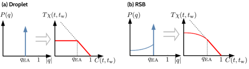
Figure 9: Sketch of the shape of the expected modification of the FDT according to the droplet and RSB theories in the double limit of $t_{\mathrm{w}},t\to\infty$.

From Eq. (22), we see that the droplet and RSB theories give very different predictions about how the FDT should be modified, as sketched in Fig.9. This important result allows one to the determine the pdf of the overlap experimentally, despite the impossibility of measuring it directly. Such an experiment was conducted by Hérisson and Ocio [111] by measuring the nonlinear fluctuation-dissipation relation between $C$ and $\chi$. Many numerical works have explored these relations in simulations of Ising spin glass models [10, 110, 112, 113, 15] and beyond [114]. All these experimental and numerical works describe a modification of the equilibrium FDT similar to that shown in Fig. 10(a) (obtained with the Janus I and II supercomputers[15]), which is extremely similar to the RSB prediction sketched in Fig. 9(b).

However it is important to recall that the connection between the equilibrium $P(q)$, and $S[C(t+t_{\mathrm{w}},t_{\mathrm{w}})]$ only holds in the limit $t_{\mathrm{w}},t\to\infty$. It is also clear from Fig. 10(a) that the current data is in a pre-asymptotic regime, because the data for different values of $t_{\mathrm{w}}$ do not superimpose, so one can not distinguish unambiguously between the droplet and RSB theories in the $t_{\mathrm{w}}\to\infty$ limit. The same applies to the experimental data. This means that, as discussed above, short $t_{\mathrm{w}}$ aging simulations and experiments are consistent with RSB, but cannot rule out the possibility that the droplet model describes the experimentally unachievable $t_{\mathrm{w}}\to\infty$ limit.

However, it has been observed that the expected relation between $S$ and the equilibrium $P(q)$ still holds at finite $t_{\mathrm{w}}$, replacing $P(q)$ by $P(q,L)$, the equilibrium pdf of the overlap in a finite system of size $L$ [15]. Indeed, Fig. 10(b) shows

$$S(C,L)=\int_{C}^{1}\mathrm{d}\,C^{\prime}\,x(C^{\prime},L)\,,\qquad\mathrm{where}\ \ x(C,L)=\int_{0}^{C}\,\mathrm{d}q\,2P(q,L)$$ (23)

obtained using the numerical equilibrium data of $P(q,L)$ (already discussed in Fig. 1), for different $L$. The similarity between the two panels of Fig. 10 is striking since the left panel is for a non-equilibrium situation on a large system, while the right panel is for equilibrium behavior on fairly small systems.

This discussion can be made more quantitative if we now bring into play $\xi(t_{\mathrm{w}})$, the size of the glassy domains in the non-equilibrium system that grows with time as the system ages. One can use the known growth of $\xi(t_{\mathrm{w}})$ (shown in Fig. 7), to predict the observed data from the equilibrium $S(C,L_{\mathrm{eff}})$ with $L_{\mathrm{eff}}(t+t_{\mathrm{w}};t_{\mathrm{w}})$ being a function of $\xi(t_{\mathrm{w}})$ and $\xi(t+t_{\mathrm{w}})$. This prediction is shown by the lines in Fig. 10(a) and the agreement with the original data (dots) is very good.

\begin{overpic}[width=208.13574pt]{FIGURES/fig_Giorgio_FDTdyn.pdf} \put(55.0,65.0){{\bf(a)}} \end{overpic}

\begin{overpic}[width=208.13574pt]{FIGURES/fig_S_C_L.pdf} \put(55.0,65.0){{\bf(b)}} \end{overpic}

Figure 10: (a) The dots show the response function $T\chi(t+t_{\mathrm{w}},t_{\mathrm{w}})$ versus $C(t+t_{\mathrm{w}},t_{\mathrm{w}})$ at $T=0.7$ for different fixed $t_{\mathrm{w}}$. Upon relaxing at fixed $t_{\mathrm{w}}$, $C(t+t_{\mathrm{w}},t_{\mathrm{w}})$ monotonically decreases from $C=1$ at $t=0$ to $C=0$ at $t=\infty$. In (b) we show the equilibrium $S(C,L)$ versus $C$ for different system sizes obtained using Eq. (23) and $P(q,L)$ extracted in independent equilibrium studies. This lines are guides to the eye. In (a) the lines are obtained by plotting the $S(C,L_{\mathrm{eff}})$ shown in (b) for an effective size, $L_{\mathrm{eff}}=\xi(t+t_{\mathrm{w}},t_{\mathrm{w}})g\left(\xi(t+t_{\mathrm{w}},t_{\mathrm{w}})/\xi(t_{\mathrm{w}})\right)$, where $g(\cdot)$ is an Ansatz function that controls the crossover between the $\xi(t_{\mathrm{w}})$ and $\xi(t+t_{\mathrm{w}})$ dominated regimes. Figures adapted from [15].

4 Statics-dynamics dictionary and relation to experiments

We have argued above that there is a quantitative equivalence between the relaxation and response of an infinite system at finite $t_{\mathrm{w}}$ [and coherence length $\xi(t_{\mathrm{w}})$] and the equilibrium properties of a system of finite size $L$. Moreover, it is possible to show that $L\sim k\xi(t_{\mathrm{w}})$, with $k\sim 4$ [15].

The existence of such a dictionary between equilibrium and non-equilibrium physics had also been explored and confirmed in previous works [115, 11, 57, 13], and tells us that the key to describing real experiments may not be in the physics of $L\to\infty$ equilibrium systems, but in that of much more modest sizes.

The question that naturally comes to mind is how much $\xi(t_{\mathrm{w}})$ differs in simulations and experiments. The answer is not very much. The current experimental world record for the largest $\xi(t_{\mathrm{w}})$, see Fig. 11, is larger than the numerical one in Fig. 7(b) by a factor $\simeq 15$. Thus the extrapolations needed to compare experiments with current simulations, if expressed in terms of $\xi(t_{\mathrm{w}})$ rather than time, are quite mild.

In fact there is an even better quantity than $\xi(t_{\mathrm{w}})$ to study when extrapolating from simulations to experiment. Roughly speaking we have $\xi(t_{\mathrm{w}})=At_{\mathrm{w}}^{T/(T_{\mathrm{c}}z_{\mathrm{c}})}$. However, the data does not actually fit a power law well so it is more convenient to consider the slope on a log-log plot, which is called the aging rate, $z_{\mathrm{c}}(T,\xi)=(T/T_{\mathrm{c}})\mathrm{d}\log t_{\mathrm{w}}/\mathrm{d}\log\xi$. It is found that $z_{c}$ is not constant but increases as $\xi(t_{\mathrm{w}})$ increases. Nonetheless, it is the most useful quantity with which to extrapolate between simulations and experimental results.

One example of such extrapolation is shown in Fig. 11 which is taken from [17] (other successful extrapolations can be found in [97, 18, 19]). Fitting the data in the figure to a straight line gives [17] $z_{\mathrm{c}}=12.37\pm 1.07$. Simulation results for $z_{c}(T,\xi)$ have been obtained for a range of waiting times and temperatures [97]. For example, at the smallest correlation length, $z_{c}\simeq 6.7$. By fitting these simulation results as described in Ref. [17] one can extrapolate the values for $z_{c}$ to the larger coherence lengths in experiment, getting $z_{c}(180.26a_{0})=11.94\pm 0.08,z_{c}(238.34a_{0})=12.76\pm 0.08$, which is in excellent agreement with value from the experimental data itself. Furthermore, combining the extrapolated aging-rate with an additional input from experiment, namely $\xi(t_{\mathrm{w}}=2750\,\text{s})$, the curve $\xi(t_{\mathrm{w}})$ could be predicted [the two dashed lines in fig:simulationsmeetexperiments encompass the experimental error for $\xi(t_{\mathrm{w}}=2750\,\text{s})$].

In summary, the statics-dynamics dictionary tells us that the dynamics of experimental spin glasses is described by the equilibrium properties of systems of size $L\sim 100$ lattice spacings. Hence the droplet-RSB dispute is irrelevant in this context since it applies to $L=\infty$. At the length scales that are relevant to experiments the data is better described by RSB theory.

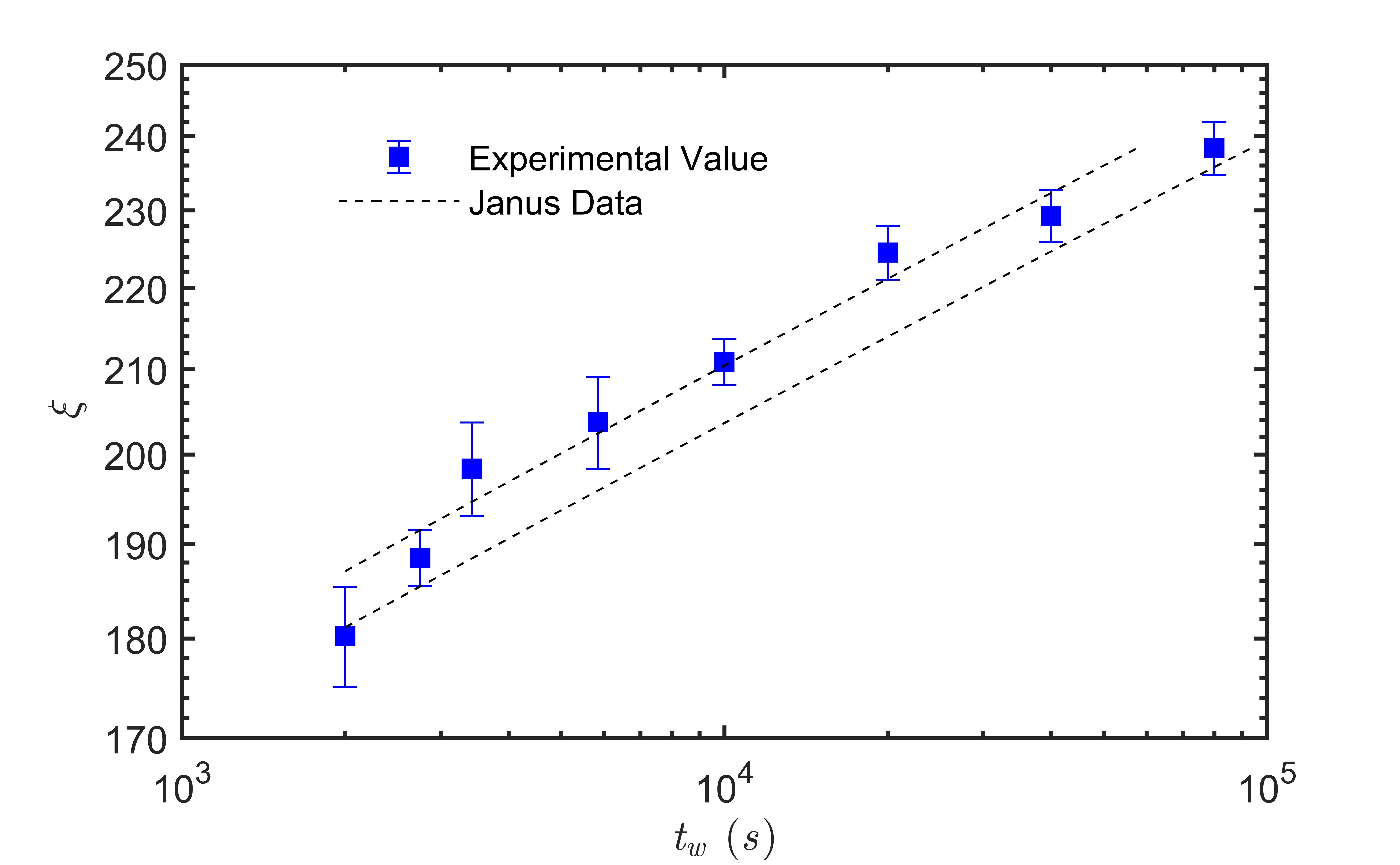
Figure 11: Coherence length $\xi(t_{\mathrm{w}})$ in units of the average distance between magnetic moments ($0.64\,\mathrm{nm}$) versus waiting time $t_{\mathrm{w}}$, as measured in a CuMn single crystal at $T\approx 0.89T_{\mathrm{c}}$. The extrapolation from Janus II data at smaller $\xi(t_{\mathrm{w}})$ is enclosed by the two dashed lines (the separation between the lines is the uncertainty in the extrapolation). Figure taken from Ref. [17].

6 Conclusions

The aim of this chapter has been to summarize what numerical simulations tell us concerning the applicability of RSB to short-range spin glasses, most particularly to $D=3$. We have seen that the situation is somewhat complicated because it appears to depend on whether or not an external magnetic field is applied.

In zero field, large-scale simulations with a dedicated processor find behavior in $D=3$ which is well described by RSB, both in equilibrium and non-equilibrium situations. The non-equilibrium simulations are found to be consistent with recent experiments on single crystals.

While the droplet picture can not be excluded as a description of spin glasses in the thermodynamic limit, if this is the case it can only apply on length and time scales far beyond the reach of simulations and experiments.

In a field, RSB predicts a spin glass phase and a dAT line, see Fig. 4, whereas the droplet picture predicts no dAT line. Numerically it has been hard to find evidence for a dAT line in $D=3$, and the situation is ambiguous in $D=4$. Numerics does, however, indicate the presence of a dAT line in high dimension. A possible explanation of these results is that $D_{\ell}^{h}$, the lower critical dimension, the dimension below which there is no transition, is greater than $3$ in the presence of a magnetic field, which is different from the case of zero field where $D_{\ell}\simeq 2.5$.

7 Acknowledgments

This work was partly supported by grants No. PID2020-112936GB-I00 and No. PGC2018-094684-B-C21 funded by Ministerio de Economía y Competitividad, Agencia Estatal de Investigación and Fondo Europeo de Desarrollo Regional (FEDER) (Spain and European Union), by grants No. GR21014 and No. IB20079 (partially funded by FEDER) funded by Junta the Extremadura (Spain), and by the Atracción de Talento program (Ref. 2019-T1/TIC-12776) funded by Comunidad de Madrid and Universidad Complutense de Madrid (Spain).

References

- [1] M. Mézard, G. Parisi, and M. Virasoro, Spin-Glass Theory and Beyond. (World Scientific, Singapore, 1987). 10.1142/0271.
- [2] E. Marinari, G. Parisi, F. Ricci-Tersenghi, J. J. Ruiz-Lorenzo, and F. Zuliani, Replica symmetry breaking in short-range spin glasses: Theoretical foundations and numerical evidences, J. Stat. Phys. 98, 973, (2000). 10.1023/A:1018607809852.
- [3] W. L. McMillan, Scaling theory of Ising spin glasses, J. Phys. C: Solid State Phys. 17, 3179, (1984). 10.1088/0022-3719/17/18/010.
- [4] A. J. Bray and M. A. Moore. Scaling theory of the ordered phase of spin glasses. In eds. J. L. van Hemmen and I. Morgenstern, Heidelberg Colloquium on Glassy Dynamics, number 275 in Lecture Notes in Physics. Springer, Berlin, (1987).
- [5] D. S. Fisher and D. A. Huse, Ordered phase of short-range Ising spin-glasses, Phys. Rev. Lett. 56, 1601 (Apr, 1986). 10.1103/PhysRevLett.56.1601. URL http://link.aps.org/doi/10.1103/PhysRevLett.56.1601.
- [6] D. S. Fisher and D. A. Huse, Nonequilibrium dynamics of spin glasses, Phys. Rev. B. 38, 373–385 (Jul, 1988). 10.1103/PhysRevB.38.373. URL https://link.aps.org/doi/10.1103/PhysRevB.38.373.
- [7] Gardner, E., A spin glass model on a hierarchical lattice, J. Phys. France. 45(11), 1755–1763, (1984). 10.1051/jphys:0198400450110175500. URL https://doi.org/10.1051/jphys:0198400450110175500.
- [8] F. Krzakala and O. C. Martin, Spin and link overlaps in three-dimensional spin glasses, Phys. Rev. Lett. 85, 3013, (2000). 10.1103/PhysRevLett.85.3013.
- [9] M. Palassini and A. P. Young, Nature of the spin glass state, Phys. Rev. Lett. 85, 3017–3020 (Oct, 2000). 10.1103/PhysRevLett.85.3017. URL https://link.aps.org/doi/10.1103/PhysRevLett.85.3017.
- [10] S. Franz, M. Mézard, G. Parisi, and L. Peliti, Measuring equilibrium properties in aging systems, Phys. Rev. Lett. 81, 1758–1761 (Aug, 1998). 10.1103/PhysRevLett.81.1758. URL http://link.aps.org/doi/10.1103/PhysRevLett.81.1758.
- [11] F. Belletti, M. Cotallo, A. Cruz, L. A. Fernandez, A. Gordillo-Guerrero, M. Guidetti, A. Maiorano, F. Mantovani, E. Marinari, V. Martín-Mayor, A. M. Sudupe, D. Navarro, G. Parisi, S. Perez-Gaviro, J. J. Ruiz-Lorenzo, S. F. Schifano, D. Sciretti, A. Tarancon, R. Tripiccione, J. L. Velasco, and D. Yllanes, Nonequilibrium spin-glass dynamics from picoseconds to one tenth of a second, Phys. Rev. Lett. 101, 157201, (2008). 10.1103/PhysRevLett.101.157201.
- [12] F. Belletti, A. Cruz, L. Fernandez, A. Gordillo-Guerrero, M. Guidetti, A. Maiorano, F. Mantovani, E. Marinari, V. Martin-Mayor, J. Monforte, et al., An in-depth view of the microscopic dynamics of Ising spin glasses at fixed temperature, Journal of Statistical Physics. 135(5), 1121–1158, (2009). 10.1007/s10955-009-9727-z.
- [13] R. Alvarez Baños, A. Cruz, L. A. Fernandez, J. M. Gil-Narvion, A. Gordillo-Guerrero, M. Guidetti, A. Maiorano, F. Mantovani, E. Marinari, V. Martín-Mayor, J. Monforte-Garcia, A. Muñoz Sudupe, D. Navarro, G. Parisi, S. Perez-Gaviro, J. J. Ruiz-Lorenzo, S. F. Schifano, B. Seoane, A. Tarancon, R. Tripiccione, and D. Yllanes, Static versus dynamic heterogeneities in the Edwards-Anderson-Ising spin glass, Phys. Rev. Lett. 105, 177202, (2010). 10.1103/PhysRevLett.105.177202.
- [14] M. Wittmann and A. P. Young, The connection between statics and dynamics of spin glasses, Journal of Statistical Mechanics: Theory and Experiment. 2016(1), 013301, (2016). URL http://stacks.iop.org/1742-5468/2016/i=1/a=013301.
- [15] M. Baity-Jesi, E. Calore, A. Cruz, L. A. Fernandez, J. M. Gil-Narvión, A. Gordillo-Guerrero, D. Iñiguez, A. Maiorano, E. Marinari, V. Martin-Mayor, J. Monforte-Garcia, A. Muñoz Sudupe, D. Navarro, G. Parisi, S. Perez-Gaviro, F. Ricci-Tersenghi, J. J. Ruiz-Lorenzo, S. F. Schifano, B. Seoane, A. Tarancón, R. Tripiccione, and D. Yllanes, A statics-dynamics equivalence through the fluctuation–dissipation ratio provides a window into the spin-glass phase from nonequilibrium measurements, Proceedings of the National Academy of Sciences. 114(8), 1838–1843, (2017). 10.1073/pnas.1621242114. URL http://www.pnas.org/content/114/8/1838.abstract.
- [16] M. Baity-Jesi, E. Calore, A. Cruz, L. A. Fernandez, J. M. Gil-Narvion, I. Gonzalez-Adalid Pemartin, A. Gordillo-Guerrero, D. Iñiguez, A. Maiorano, E. Marinari, V. Martin-Mayor, J. Moreno-Gordo, A. Muñoz Sudupe, D. Navarro, I. Paga, G. Parisi, S. Perez-Gaviro, F. Ricci-Tersenghi, J. J. Ruiz-Lorenzo, S. F. Schifano, B. Seoane, A. Tarancon, R. Tripiccione, and D. Yllanes, Temperature chaos is present in off-equilibrium spin-glass dynamics, Communications physics. 4(1), 74, (2021). ISSN 2399-3650. 10.1038/s42005-021-00565-9. URL https://doi.org/10.1038/s42005-021-00565-9.
- [17] Q. Zhai, V. Martin-Mayor, D. L. Schlagel, G. G. Kenning, and R. L. Orbach, Slowing down of spin glass correlation length growth: Simulations meet experiments, Phys. Rev. B. 100, 094202 (Sep, 2019). 10.1103/PhysRevB.100.094202. URL https://link.aps.org/doi/10.1103/PhysRevB.100.094202.
- [18] Q. Zhai, I. Paga, M. Baity-Jesi, E. Calore, A. Cruz, L. A. Fernandez, J. M. Gil-Narvion, I. Gonzalez-Adalid Pemartin, A. Gordillo-Guerrero, D. Iñiguez, A. Maiorano, E. Marinari, V. Martin-Mayor, J. Moreno-Gordo, A. Muñoz Sudupe, D. Navarro, R. L. Orbach, G. Parisi, S. Perez-Gaviro, F. Ricci-Tersenghi, J. J. Ruiz-Lorenzo, S. F. Schifano, D. L. Schlagel, B. Seoane, A. Tarancon, R. Tripiccione, and D. Yllanes, Scaling law describes the spin-glass response in theory, experiments, and simulations, Phys. Rev. Lett. 125, 237202 (Nov, 2020). 10.1103/PhysRevLett.125.237202. URL https://link.aps.org/doi/10.1103/PhysRevLett.125.237202.
- [19] I. Paga, Q. Zhai, M. Baity-Jesi, E. Calore, A. Cruz, L. A. Fernandez, J. M. Gil-Narvion, I. Gonzalez-Adalid Pemartin, A. Gordillo-Guerrero, D. Iñiguez, A. Maiorano, E. Marinari, V. Martin-Mayor, J. Moreno-Gordo, A. Muñoz-Sudupe, D. Navarro, R. L. Orbach, G. Parisi, S. Perez-Gaviro, F. Ricci-Tersenghi, J. J. Ruiz-Lorenzo, S. F. Schifano, D. L. Schlagel, B. Seoane, A. Tarancon, R. Tripiccione, and D. Yllanes, Spin-glass dynamics in the presence of a magnetic field: exploration of microscopic properties, Journal of Statistical Mechanics: Theory and Experiment. 2021(3), 033301 (mar, 2021). 10.1088/1742-5468/abdfca. URL https://doi.org/10.1088/1742-5468/abdfca.
- [20] H. Kawamura, Chiral ordering in Heisenberg spin glasses in two and three dimensions, Phys. Rev. Lett. 68, 3785–3788 (Jun, 1992). 10.1103/PhysRevLett.68.3785. URL http://link.aps.org/doi/10.1103/PhysRevLett.68.3785.
- [21] H. Kawamura, Dynamical simulation of spin-glass and chiral-glass orderings in three-dimensional Heisenberg spin glasses, Phys. Rev. Lett. 80, 5421–5424 (Jun, 1998). 10.1103/PhysRevLett.80.5421. URL http://link.aps.org/doi/10.1103/PhysRevLett.80.5421.
- [22] H. Kawamura and M. S. Li, Nature of the ordering in the three-dimensional spin glass, Phys. Rev. Lett. 87, 187204 (Oct, 2001). 10.1103/PhysRevLett.87.187204. URL https://link.aps.org/doi/10.1103/PhysRevLett.87.187204.
- [23] H. Kawamura, Fluctuation-dissipation ratio of the Heisenberg spin glass, Phys. Rev. Lett. 90, 237201 (Jun, 2003). 10.1103/PhysRevLett.90.237201. URL http://link.aps.org/doi/10.1103/PhysRevLett.90.237201.
- [24] T. Ogawa, K. Uematsu, and H. Kawamura, Monte Carlo studies of the spin-chirality decoupling in the three-dimensional Heisenberg spin glass, Phys. Rev. B. 101, 014434 (Jan, 2020). 10.1103/PhysRevB.101.014434. URL https://link.aps.org/doi/10.1103/PhysRevB.101.014434.
- [25] L. A. Fernandez, V. Martín-Mayor, S. Perez-Gaviro, A. Tarancon, and A. P. Young, Phase transition in the three dimensional Heisenberg spin glass: Finite-size scaling analysis, Phys. Rev. B. 80, 024422, (2009). 10.1103/PhysRevB.80.024422.
- [26] I. Campos, M. Cotallo-Aban, V. Martin-Mayor, S. Perez-Gaviro, and A. Tarancon, Spin-glass transition of the three-dimensional Heisenberg spin glass, Phys. Rev. Lett. 97, 217204 (Nov, 2006). 10.1103/PhysRevLett.97.217204. URL https://link.aps.org/doi/10.1103/PhysRevLett.97.217204.
- [27] L. W. Lee and A. P. Young, Single spin and chiral glass transition in vector spin glasses in three dimensions, Phys. Rev. Lett. 90, 227203 (Jun, 2003). 10.1103/PhysRevLett.90.227203. URL https://link.aps.org/doi/10.1103/PhysRevLett.90.227203.
- [28] A. J. Bray and M. A. Moore, Is mean-field theory valid for spin glasses?, J. Phys. C. 15, 3897, (1982). 10.1088/0022-3719/15/18/007.
- [29] M. Baity-Jesi, L. A. Fernandez, V. Martín-Mayor, and J. M. Sanz, Phase transition in three-dimensional Heisenberg spin glasses with strong random anisotropies through a multi-GPU parallelization, Phys. Rev. 89, 014202, (2014). 10.1103/PhysRevB.89.014202.
- [30] M. Baity-Jesi, R. A. Baños, A. Cruz, L. A. Fernandez, J. M. Gil-Narvion, A. Gordillo-Guerrero, D. Iniguez, A. Maiorano, F. Mantovani, E. Marinari, V. Martín-Mayor, J. Monforte-Garcia, A. Muñoz Sudupe, D. Navarro, G. Parisi, S. Perez-Gaviro, M. Pivanti, F. Ricci-Tersenghi, J. J. Ruiz-Lorenzo, S. F. Schifano, B. Seoane, A. Tarancon, R. Tripiccione, and D. Yllanes, Critical parameters of the three-dimensional Ising spin glass, Phys. Rev. B. 88, 224416, (2013). 10.1103/PhysRevB.88.224416.
- [31] Bouchiat, H., Determination of the critical exponents in the AgMn spin glass, J. Phys. France. 47(1), 71–88, (1986). 10.1051/jphys:0198600470107100. URL https://doi.org/10.1051/jphys:0198600470107100.
- [32] G. Parisi, Field Theory, Disorder and Simulations. (World Scientific, 1994).
- [33] G. Toulouse, Theory of the frustration effect in spin glasses, Communications on Physics. 2, 115, (1977).
- [34] J. R. L. de Almeida and D. J. Thouless, Stability of the Sherrington-Kirkpatrick solution of a spin glass model, J. Phys. A: Math. Gen. 11, 983, (1978). 10.1088/0305-4470/11/5/028. URL http://stacks.iop.org/0305-4470/11/i=5/a=028.
- [35] C. de Dominicis and I. Giardina, Random Fields and Spin Glasses: a field theory approach. (Cambridge University Press, Cambridge, England, 2006).
- [36] G. Parisi and T. Rizzo, Critical dynamics in glassy systems, Phys. Rev. E. 87, 012101 (Jan, 2013). 10.1103/PhysRevE.87.012101. URL https://link.aps.org/doi/10.1103/PhysRevE.87.012101.
- [37] L. A. Fernandez, I. Gonzalez-Adalid Pemartin, V. Martin-Mayor, G. Parisi, F. Ricci-Tersenghi, T. Rizzo, J. J. Ruiz-Lorenzo, and M. Veca, Numerical test of the replica-symmetric hamiltonian for correlations of the critical state of spin glasses in a field, Phys. Rev. E. 105, 054106 (May, 2022). 10.1103/PhysRevE.105.054106. URL https://link.aps.org/doi/10.1103/PhysRevE.105.054106.
- [38] D. J. Amit and V. Martín-Mayor, Field Theory, the Renormalization Group and Critical Phenomena. (World Scientific, Singapore, 2005), third edition. 10.1142/9789812775313_bmatter. URL http://www.worldscientific.com/worldscibooks/10.1142/5715.
- [39] M. Palassini and S. Caracciolo, Universal finite-size scaling functions in the 3D Ising spin glass, Phys. Rev. Lett. 82, 5128–5131, (1999). 10.1103/PhysRevLett.82.5128.
- [40] H. G. Ballesteros, A. Cruz, L. A. Fernandez, V. Martín-Mayor, J. Pech, J. J. Ruiz-Lorenzo, A. Tarancon, P. Tellez, C. L. Ullod, and C. Ungil, Critical behavior of the three-dimensional Ising spin glass, Phys. Rev. B. 62, 14237–14245, (2000). 10.1103/PhysRevB.62.14237.
- [41] L. Leuzzi, G. Parisi, F. Ricci-Tersenghi, and J. J. Ruiz-Lorenzo, Ising spin-glass transition in a magnetic field outside the limit of validity of mean-field theory, Phys. Rev. Lett. 103, 267201, (2009). 10.1103/PhysRevLett.103.267201.
- [42] R. A. Baños, A. Cruz, L. A. Fernandez, J. M. Gil-Narvion, A. Gordillo-Guerrero, M. Guidetti, D. Iniguez, A. Maiorano, E. Marinari, V. Martín-Mayor, J. Monforte-Garcia, A. Muñoz Sudupe, D. Navarro, G. Parisi, S. Perez-Gaviro, J. J. Ruiz-Lorenzo, S. F. Schifano, B. Seoane, A. Tarancon, P. Tellez, R. Tripiccione, and D. Yllanes, Thermodynamic glass transition in a spin glass without time-reversal symmetry, Proc. Natl. Acad. Sci. USA. 109, 6452, (2012). 10.1073/pnas.1203295109.
- [43] F. Barahona, On the computational complexity of Ising spin glass models, Journal of Physics A: Mathematical and General. 15(10), 3241, (1982). 10.1088/0305-4470/15/10/028. URL http://stacks.iop.org/0305-4470/15/i=10/a=028.
- [44] K. Hukushima and K. Nemoto, Exchange Monte Carlo method and application to spin glass simulations, J. Phys. Soc. Japan. 65, 1604, (1996). 10.1143/JPSJ.65.1604.
- [45] E. Marinari. Optimized Monte Carlo methods. In eds. J. Kerstész and I. Kondor, Advances in Computer Simulation. Springer-Verlag, (1998). 10.1007/BFb0105459.
- [46] R. H. Swendsen and J.-S. Wang, Nonuniversal critical dynamics in Monte Carlo simulations, Phys. Rev. Lett. 58, 86–88 (Jan, 1987). 10.1103/PhysRevLett.58.86. URL https://link.aps.org/doi/10.1103/PhysRevLett.58.86.
- [47] R. H. Swendsen and J.-S. Wang, Replica Monte Carlo simulation of spin-glasses, Phys. Rev. Lett. 57, 2607–2609 (Nov, 1986). 10.1103/PhysRevLett.57.2607. URL https://link.aps.org/doi/10.1103/PhysRevLett.57.2607.
- [48] J.-S. Wang and R. Swendsen, Replica Monte Carlo simulation (revisited), Prog. Theo. Phys. Supplement. 157, 317, (2005).
- [49] J. Houdayer, A cluster Monte Carlo algorithm for 2-dimensional spin glasses, Euro. Phys. Journal B. 22, 479, (2001). 10.1007/PL00011151.
- [50] L. A. Fernandez, V. Martín-Mayor, G. Parisi, and B. Seoane, Temperature chaos in 3d Ising spin glasses is driven by rare events, EPL. 103(6), 67003, (2013). 10.1209/0295-5075/103/67003.
- [51] A. Billoire, L. A. Fernandez, A. Maiorano, E. Marinari, V. Martin-Mayor, J. Moreno-Gordo, G. Parisi, F. Ricci-Tersenghi, and J. J. Ruiz-Lorenzo, Dynamic variational study of chaos: spin glasses in three dimensions, Journal of Statistical Mechanics: Theory and Experiment. 2018(3), 033302, (2018). 10.1088/1742-5468/aaa387. URL http://stacks.iop.org/1742-5468/2018/i=3/a=033302.
- [52] V. Martín-Mayor and I. Hen, Unraveling quantum annealers using classical hardness, Scientific Reports. 5, 15324 (October, 2015). 10.1038/srep15324.
- [53] A. T. Ogielski, Dynamics of three-dimensional Ising spin glasses in thermal equilibrium, Phys. Rev. B. 32, 7384, (1985). 10.1103/PhysRevB.32.7384.
- [54] A. Cruz, J. Pech, A. Tarancon, P. Tellez, C. L. Ullod, and C. Ungil, SUE: A special purpose computer for spin glass models, Comp. Phys. Comm. 133, 165–176, (2001). 10.1016/S0010-4655(00)00170-3.
- [55] F. Belletti, M. Cotallo, A. Cruz, L. A. Fernandez, A. Gordillo, A. Maiorano, F. Mantovani, E. Marinari, V. Martín-Mayor, A. Muñoz Sudupe, D. Navarro, S. Perez-Gaviro, J. J. Ruiz-Lorenzo, S. F. Schifano, D. Sciretti, A. Tarancon, R. Tripiccione, and J. L. Velasco, Simulating spin systems on IANUS, an FPGA-based computer, Comp. Phys. Comm. 178, 208–216, (2008). 10.1016/j.cpc.2007.09.006.
- [56] M. Baity-Jesi, R. A. Baños, A. Cruz, L. A. Fernandez, J. M. Gil-Narvion, A. Gordillo-Guerrero, D. Iniguez, A. Maiorano, F. Mantovani, E. Marinari, V. Martín-Mayor, J. Monforte-Garcia, A. Muñoz Sudupe, D. Navarro, G. Parisi, S. Perez-Gaviro, M. Pivanti, F. Ricci-Tersenghi, J. J. Ruiz-Lorenzo, S. F. Schifano, B. Seoane, A. Tarancon, R. Tripiccione, and D. Yllanes, Janus II: a new generation application-driven computer for spin-system simulations, Comp. Phys. Comm. 185, 550–559, (2014). 10.1016/j.cpc.2013.10.019.
- [57] R. Alvarez Baños, A. Cruz, L. A. Fernandez, J. M. Gil-Narvion, A. Gordillo-Guerrero, M. Guidetti, A. Maiorano, F. Mantovani, E. Marinari, V. Martín-Mayor, J. Monforte-Garcia, A. Muñoz Sudupe, D. Navarro, G. Parisi, S. Perez-Gaviro, J. J. Ruiz-Lorenzo, S. F. Schifano, B. Seoane, A. Tarancon, R. Tripiccione, and D. Yllanes, Nature of the spin-glass phase at experimental length scales, J. Stat. Mech. 2010, P06026, (2010). 10.1088/1742-5468/2010/06/P06026.
- [58] S. Boettcher, Stiffness of the Edwards-Anderson model in all dimensions, Phys. Rev. Lett. 95, 197205 (Nov, 2005). 10.1103/PhysRevLett.95.197205. URL http://link.aps.org/doi/10.1103/PhysRevLett.95.197205.
- [59] J. D. Reger, R. N. Bhatt, and A. P. Young, Monte Carlo study of the order-parameter distribution in the four-dimensional Ising spin glass, Phys. Rev. Lett. 64, 1859–1862 (Apr, 1990). 10.1103/PhysRevLett.64.1859. URL https://link.aps.org/doi/10.1103/PhysRevLett.64.1859.
- [60] B. A. Berg and W. Janke, Multioverlap simulations of the 3d Edwards-Anderson Ising spin glass, Phys. Rev. Lett. 80, 4771–4774 (May, 1998). 10.1103/PhysRevLett.80.4771. URL https://link.aps.org/doi/10.1103/PhysRevLett.80.4771.
- [61] E. Marinari, G. Parisi, and J. J. Ruiz-Lorenzo, Phase structure of the three-dimensional Edwards-Anderson spin glass, Phys. Rev. B. 58, 14852–14863 (Dec, 1998). 10.1103/PhysRevB.58.14852. URL https://link.aps.org/doi/10.1103/PhysRevB.58.14852.
- [62] H. G. Katzgraber, M. Palassini, and A. P. Young, Monte Carlo simulations of spin glasses at low temperatures, Phys. Rev. B. 63, 184422 (Apr, 2001). 10.1103/PhysRevB.63.184422. URL https://link.aps.org/doi/10.1103/PhysRevB.63.184422.
- [63] H. G. Katzgraber and A. P. Young, Monte Carlo simulations of spin glasses at low temperatures: Effects of free boundary conditions, Phys. Rev. B. 65, 214402 (May, 2002). 10.1103/PhysRevB.65.214402. URL https://link.aps.org/doi/10.1103/PhysRevB.65.214402.
- [64] B. A. Berg, A. Billoire, and W. Janke, Overlap distribution of the three-dimensional Ising model, Phys. Rev. E. 66, 046122 (Oct, 2002). 10.1103/PhysRevE.66.046122. URL https://link.aps.org/doi/10.1103/PhysRevE.66.046122.
- [65] W. Wang, M. Wallin, and J. Lidmar, Evidence of many thermodynamic states of the three-dimensional Ising spin glass, Phys. Rev. Research. 2, 043241 (Nov, 2020). 10.1103/PhysRevResearch.2.043241. URL https://link.aps.org/doi/10.1103/PhysRevResearch.2.043241.
- [66] E. Marinari, G. Parisi, F. Ricci-Tersenghi, and J. J. Ruiz-Lorenzo, Small window overlaps are effective probes of replica symmetry breaking in 3d spin glasses, Journal of Physics A: Math. and Gen. 31, L481, (1998). 10.1088/0305-4470/31/26/001.
- [67] P. Contucci, C. Giardinà, C. Giberti, and C. Vernia, Overlap equivalence in the Edwards-Anderson model, Phys. Rev. Lett. 96, 217204 (Jun, 2006). 10.1103/PhysRevLett.96.217204. URL https://link.aps.org/doi/10.1103/PhysRevLett.96.217204.
- [68] F. Guerra, About the overlap distribution in mean field spin glass models, International Journal of Modern Physics B. 10, 1675, (1996). 10.1142/S0217979296000751.
- [69] S. Ghirlanda and F. Guerra, General properties of overlap probability distributions in disordered spin systems. towards parisi ultrametricity, Journal of Physics A: Mathematical and General. 31(46), 9149–9155 (nov, 1998). 10.1088/0305-4470/31/46/006. URL https://doi.org/10.1088/0305-4470/31/46/006.
- [70] M. Aizenman and P. Contucci, On the stability of the quenched state in mean-field spin-glass models, J. Stat. Phys. 92, 765, (1998). https://doi.org/10.1023/A:1023080223894. URL https://link.springer.com/article/10.1023/A:1023080223894.
- [71] G. Parisi and F. Ricci-Tersenghi, On the origin of ultrametricity, J. Phys. A: Math. Gen. 33, 113, (2000). 10.1088/0305-4470/33/1/307.
- [72] D. Iñiguez, G. Parisi, and J. J. Ruiz-Lorenzo, Simulation of three-dimensional Ising spin glass model using three replicas: study of Binder cumulants, J. Phys. A: Math. and Gen. 29, 4337, (1996). 10.1088/0305-4470/29/15/009.
- [73] G. Parisi, Spin glass models from the point of view of spin distributions, Ann. Prob. 41, 1315, (2013). 10.1214/11-AOP696.
- [74] G. Hed, A. P. Young, and E. Domany, Lack of ultrametricity in the low-temperature phase of three-dimensional Ising spin glasses, Phys. Rev. Lett. 92, 157201 (Apr, 2004). 10.1103/PhysRevLett.92.157201. URL https://link.aps.org/doi/10.1103/PhysRevLett.92.157201.
- [75] R. A. Baños, A. Cruz, L. A. Fernandez, J. M. Gil-Narvion, A. Gordillo-Guerrero, M. Guidetti, D. Iñiguez, A. Maiorano, F. Mantovani, E. Marinari, V. Martín-Mayor, J. Monforte-Garcia, A. Muñoz Sudupe, D. Navarro, G. Parisi, S. Perez-Gaviro, F. Ricci-Tersenghi, J. J. Ruiz-Lorenzo, S. F. Schifano, B. Seoane, A. Tarancón, R. Tripiccione, and D. Yllanes, Sample-to-sample fluctuations of the overlap distributions in the three-dimensional Edwards-Anderson spin glass, Phys. Rev. B. 84, 174209 (Nov, 2011). 10.1103/PhysRevB.84.174209. URL http://link.aps.org/doi/10.1103/PhysRevB.84.174209.
- [76] D. Sherrington and S. Kirkpatrick, Solvable model of a spin-glass, Phys. Rev. Lett. 35, 1792–1796 (Dec, 1975). 10.1103/PhysRevLett.35.1792. URL https://link.aps.org/doi/10.1103/PhysRevLett.35.1792.
- [77] G. Parisi, Infinite number of order parameters for spin-glasses, Phys. Rev. Lett. 43, 1754–1756 (Dec, 1979). 10.1103/PhysRevLett.43.1754. URL https://link.aps.org/doi/10.1103/PhysRevLett.43.1754.
- [78] G. Parisi, The order parameter for spin glasses: a function on the interval –, J. Phys. A. 13, 1101, (1980). 10.1088/0305-4470/13/3/042.
- [79] G. Parisi, Order parameter for spin-glasses, Phys. Rev. Lett. 50, 1946–1948 (Jun, 1983). 10.1103/PhysRevLett.50.1946. URL https://link.aps.org/doi/10.1103/PhysRevLett.50.1946.
- [80] G. Parisi, Statistical Field Theory. (Addison-Wesley, 1988).
- [81] S. Franz, G. Parisi, and M. Virasoro, Interfaces and lower critical dimension in a spin glass model, J. Phys. (France). 4, 1657, (1994). 10.1051/jp1:1994213.
- [82] A. Maiorano and G. Parisi, Support for the value 5/2 for the spin glass lower critical dimension at zero magnetic field, Proceedings of the National Academy of Sciences. 115(20), 5129–5134, (2018). ISSN 0027-8424. 10.1073/pnas.1720832115. URL https://www.pnas.org/content/115/20/5129.
- [83] T. Nattermann. Theory of the Random Field Ising Model. In ed. A. P. Young, Spin glasses and random fields. World Scientific, Singapore, (1998).
- [84] A. P. Young and H. G. Katzgraber, Absence of an Almeida-Thouless line in three-dimensional spin glasses, Phys. Rev. Lett. 93, 207203 (Nov, 2004). 10.1103/PhysRevLett.93.207203. URL https://link.aps.org/doi/10.1103/PhysRevLett.93.207203.
- [85] H. G. Katzgraber and A. P. Young, Probing the Almeida-Thouless line away from the mean-field model, Phys. Rev. B. 72, 184416 (Nov, 2005). 10.1103/PhysRevB.72.184416. URL https://link.aps.org/doi/10.1103/PhysRevB.72.184416.
- [86] T. Jörg, H. G. Katzgraber, and F. Krzakala, Behavior of Ising spin glasses in a magnetic field, Phys. Rev. Lett. 100, 197202, (2008). 10.1103/PhysRevLett.100.197202.
- [87] M. Baity-Jesi, R. A. Baños, A. Cruz, L. A. Fernandez, J. M. Gil-Narvion, A. Gordillo-Guerrero, D. Iniguez, A. Maiorano, M. F., E. Marinari, V. Martín-Mayor, J. Monforte-Garcia, A. Muñoz Sudupe, D. Navarro, G. Parisi, S. Perez-Gaviro, M. Pivanti, F. Ricci-Tersenghi, J. J. Ruiz-Lorenzo, S. F. Schifano, B. Seoane, A. Tarancon, R. Tripiccione, and D. Yllanes, The three dimensional Ising spin glass in an external magnetic field: the role of the silent majority, J. Stat. Mech. 2014, P05014, (2014). 10.1088/1742-5468/2014/05/P05014.
- [88] M. Hasenbusch, A. Pelissetto, and E. Vicari, Critical behavior of three-dimensional Ising spin glass models, Phys. Rev. B. 78, 214205 (Dec, 2008). 10.1103/PhysRevB.78.214205. URL https://link.aps.org/doi/10.1103/PhysRevB.78.214205.
- [89] G. Parisi and T. Temesvári, Replica symmetry breaking in and around six dimensions, Nucl. Phys. B. 858, 293, (2012). 10.1016/j.nuclphysb.2012.01.014.
- [90] J. Yeo and M. A. Moore, Critical point scaling of Ising spin glasses in a magnetic field, Phys. Rev. B. 91, 104432 (Mar, 2015). 10.1103/PhysRevB.91.104432. URL https://link.aps.org/doi/10.1103/PhysRevB.91.104432.
- [91] T. Aspelmeier, H. G. Katzgraber, D. Larson, M. A. Moore, M. Wittmann, and J. Yeo, Finite-size critical scaling in Ising spin glasses in the mean-field regime, Phys. Rev. E. 93, 032123 (Mar, 2016). 10.1103/PhysRevE.93.032123. URL https://link.aps.org/doi/10.1103/PhysRevE.93.032123.
- [92] A. J. Bray and S. A. Roberts, Renormalisation-group approach to the spin glass transition in finite magnetic fields, J. Phys. C. 13, 5405, (1980). 10.1088/0022-3719/13/29/019.
- [93] M. C. Angelini, C. Lucibello, G. Parisi, G. Perrupato, F. Ricci-Tersenghi, and T. Rizzo, Unexpected upper critical dimension for spin glass models in a field predicted by the loop expansion around the bethe solution at zero temperature, Phys. Rev. Lett. 128, 075702 (Feb, 2022). 10.1103/PhysRevLett.128.075702. URL https://link.aps.org/doi/10.1103/PhysRevLett.128.075702.
- [94] G. Parisi and F. Ricci-Tersenghi, A numerical study of the overlap probability distribution and its sample-to-sample fluctuations in a mean-field model, Phil. Mag. 92, 341, (2012). 10.1080/14786435.2011.634843.
- [95] J. Höller and N. Read, One-step replica-symmetry-breaking phase below the de Almeida–Thouless line in low-dimensional spin glasses, Phys. Rev. E. 101, 042114 (Apr, 2020). 10.1103/PhysRevE.101.042114. URL https://link.aps.org/doi/10.1103/PhysRevE.101.042114.
- [96] M. Baity-Jesi, R. A. Baños, A. Cruz, L. A. Fernandez, J. M. Gil-Narvion, A. Gordillo-Guerrero, D. Iñiguez, A. Maiorano, F. Mantovani, E. Marinari, V. Martin-Mayor, J. Monforte-Garcia, A. Muñoz Sudupe, D. Navarro, G. Parisi, S. Perez-Gaviro, M. Pivanti, F. Ricci-Tersenghi, J. J. Ruiz-Lorenzo, S. F. Schifano, B. Seoane, A. Tarancon, R. Tripiccione, and D. Yllanes, Dynamical transition in the Edwards-Anderson spin glass in an external magnetic field, Phys. Rev. E. 89, 032140 (Mar, 2014). 10.1103/PhysRevE.89.032140. URL https://link.aps.org/doi/10.1103/PhysRevE.89.032140.
- [97] M. Baity-Jesi, E. Calore, A. Cruz, L. A. Fernandez, J. M. Gil-Narvion, A. Gordillo-Guerrero, D. Iñiguez, A. Maiorano, E. Marinari, V. Martin-Mayor, J. Moreno-Gordo, A. Muñoz Sudupe, D. Navarro, G. Parisi, S. Perez-Gaviro, F. Ricci-Tersenghi, J. J. Ruiz-Lorenzo, S. F. Schifano, B. Seoane, A. Tarancon, R. Tripiccione, and D. Yllanes, Aging rate of spin glasses from simulations matches experiments, Phys. Rev. Lett. 120, 267203 (Jun, 2018). 10.1103/PhysRevLett.120.267203. URL https://link.aps.org/doi/10.1103/PhysRevLett.120.267203.
- [98] Y. G. Joh, R. Orbach, G. G. Wood, J. Hammann, and E. Vincent, Extraction of the spin glass correlation length, Phys. Rev. Lett. 82, 438–441 (Jan, 1999). 10.1103/PhysRevLett.82.438. URL https://link.aps.org/doi/10.1103/PhysRevLett.82.438.
- [99] M. Baity-Jesi, E. Calore, A. Cruz, L. A. Fernandez, J. M. Gil-Narvion, A. Gordillo-Guerrero, D. Iñiguez, A. Maiorano, E. Marinari, V. Martin-Mayor, J. Monforte-Garcia, A. Muñoz Sudupe, D. Navarro, G. Parisi, S. Perez-Gaviro, F. Ricci-Tersenghi, J. J. Ruiz-Lorenzo, S. F. Schifano, B. Seoane, A. Tarancon, R. Tripiccione, and D. Yllanes, Matching microscopic and macroscopic responses in glasses, Phys. Rev. Lett. 118, 157202 (Apr, 2017). 10.1103/PhysRevLett.118.157202. URL https://link.aps.org/doi/10.1103/PhysRevLett.118.157202.
- [100] H. Rieger. Monte Carlo studies of Ising spin glasses and random fields. In ed. D. Stauffer, Annual Reviews of Computational Physics II. World Scientific, Singapore, (1995).
- [101] E. Marinari, G. Parisi, J. Ruiz-Lorenzo, and F. Ritort, Numerical evidence for spontaneously broken replica symmetry in 3d spin glasses, Phys. Rev. Lett. 76, 843–846 (Jan, 1996). 10.1103/PhysRevLett.76.843. URL https://link.aps.org/doi/10.1103/PhysRevLett.76.843.
- [102] E. Marinari, G. Parisi, F. Ricci-Tersenghi, and Ruiz-Lorenzo, Off-equilibrium dynamics at very low temperatures in three-dimensional spin glasses, J. Phys. A: Math. Gen. 33, 2373, (2000). 10.1088/0305-4470/33/12/305.
- [103] L. Berthier and J.-P. Bouchaud, Geometrical aspects of aging and rejuvenation in the Ising spin glass: A numerical study, Physical Review B. 66(5), 054404, (2002).
- [104] L. A. Fernández and V. Martín-Mayor, Testing statics-dynamics equivalence at the spin-glass transition in three dimensions, Phys. Rev. B. 91, 174202 (May, 2015). 10.1103/PhysRevB.91.174202. URL http://link.aps.org/doi/10.1103/PhysRevB.91.174202.
- [105] S. Nakamae, C. Crauste-Thibierge, D. L’Hôte, E. Vincent, E. Dubois, V. Dupuis, and R. Perzynski, Dynamic correlation length growth in superspin glass: Bridging experiments and simulations, Applied Physics Letters. 101(24), 242409, (2012). 10.1063/1.4769840.
- [106] Q. Zhai, D. C. Harrison, D. Tennant, E. D. Dahlberg, G. G. Kenning, and R. L. Orbach, Glassy dynamics in CuMn thin-film multilayers, Phys. Rev. B. 95, 054304 (Feb, 2017). 10.1103/PhysRevB.95.054304. URL https://link.aps.org/doi/10.1103/PhysRevB.95.054304.
- [107] M. A. Moore, Droplet-scaling versus replica symmetry breaking debate in spin glasses revisited, Phys. Rev. E. 103, 062111 (Jun, 2021). 10.1103/PhysRevE.103.062111. URL https://link.aps.org/doi/10.1103/PhysRevE.103.062111.
- [108] L. F. Cugliandolo and J. Kurchan, Analytical solution of the off-equilibrium dynamics of a long-range spin-glass model, Phys. Rev. Lett. 71, 173–176 (Jul, 1993). 10.1103/PhysRevLett.71.173. URL http://link.aps.org/doi/10.1103/PhysRevLett.71.173.
- [109] S. Franz and H. Rieger, Fluctuation-dissipation ratio in three-dimensional spin glasses, Journal of statistical physics. 79(3), 749–758, (1995). 10.1007/BF02184881.
- [110] E. Marinari, G. Parisi, F. Ricci-Tersenghi, and J. J. Ruiz-Lorenzo, Violation of the fluctuation-dissipation theorem in finite-dimensional spin glasses, Journal of Physics A: Mathematical and General. 31(11), 2611, (1998). 10.1088/0305-4470/31/11/011.
- [111] D. Hérisson and M. Ocio, Fluctuation-dissipation ratio of a spin glass in the aging regime, Phys. Rev. Lett. 88, 257202 (Jun, 2002). 10.1103/PhysRevLett.88.257202. URL https://link.aps.org/doi/10.1103/PhysRevLett.88.257202.
- [112] A. Cruz, L. A. Fernández, S. Jiménez, J. J. Ruiz-Lorenzo, and A. Tarancón, Off-equilibrium fluctuation-dissipation relations in the Ising spin glass in a magnetic field, Phys. Rev. B. 67, 214425 (Jun, 2003). 10.1103/PhysRevB.67.214425. URL https://link.aps.org/doi/10.1103/PhysRevB.67.214425.
- [113] F. Ricci-Tersenghi, Measuring the fluctuation-dissipation ratio in glassy systems with no perturbing field, Phys. Rev. E. 68, 065104 (Dec, 2003). 10.1103/PhysRevE.68.065104. URL http://link.aps.org/doi/10.1103/PhysRevE.68.065104.
- [114] A. Crisanti and F. Ritort, Violation of the fluctuation–dissipation theorem in glassy systems: basic notions and the numerical evidence, Journal of Physics A: Mathematical and General. 36(21), R181, (2003). 10.1088/0305-4470/36/21/201.
- [115] A. Barrat and L. Berthier, Real-space application of the mean-field description of spin-glass dynamics, Phys. Rev. Lett. 87, 087204 (Aug, 2001). 10.1103/PhysRevLett.87.087204. URL http://link.aps.org/doi/10.1103/PhysRevLett.87.087204.