Capturing Graphs with Hypo-Elliptic Diffusions

Abstract

Convolutional layers within graph neural networks operate by aggregating information about local neighbourhood structures; one common way to encode such substructures is through random walks. The distribution of these random walks evolves according to a diffusion equation defined using the graph Laplacian. We extend this approach by leveraging classic mathematical results about hypo-elliptic diffusions. This results in a novel tensor-valued graph operator, which we call the hypo-elliptic graph Laplacian. We provide theoretical guarantees and efficient low-rank approximation algorithms. In particular, this gives a structured approach to capture long-range dependencies on graphs that is robust to pooling. Besides the attractive theoretical properties, our experiments show that this method competes with graph transformers on datasets requiring long-range reasoning but scales only linearly in the number of edges as opposed to quadratically in nodes.

1 Introduction

Obtaining a latent description of the non-Euclidean structure of a graph is central to many applications. One common approach is to construct a set of features for each node that represents the local neighborhood of this node; pooling these node features then provides a latent description of the whole graph. A classic way to arrive at such node features is by random walks: at the given node one starts a random walk, and extracts a summary of the local neighbourhood from its sample trajectories. We revisit this random walk construction and are inspired by two classical mathematical results:

Hypo-elliptic Laplacian.

In the Euclidean case of Brownian motion $B=(B_{t})_{t\geq 0}$ evolving in $\mathbb{R}^{n}$, the quantity $u(t,x)=\mathbb{E}[f(B_{t})|B_{0}=x]$ solves the heat equation $\partial_{t}u=\Delta u$ on $[0,\infty)\times\mathbb{R}^{n}$, $u(0,x)=f(x)$. Seminal work of Gaveau [gaveau_principe_1977] in the 1970s shows that if one replaces $f(B_{t})$ in the expectation by a functional of the whole trajectory, $F(B_{s}:s\in[0,t])$, then a path-dependent heat equation can be derived where the classical Laplacian $\Delta$ is replaced by the so-called hypo-elliptic Laplacian.

Free Algebras.

A simple way to capture a sequence – for us, a sequence of nodes visited by a random walk on a graph – is to associate with each sequence element an element in an algebra and multiply these algebra elements together. If the algebra multiplication is commutative, the sequential structure is lost but if it is non-commutative, this captures the order in the sequence. In fact, by using the free associative algebra, this can be done faithfully and linear functionals of this algebra correspond to functionals on the space of sequences.

We leverage these ideas from the Euclidean case of $\mathbb{R}^{d}$ to the non-Euclidean case of graphs. In particular, we construct features for a given node by sampling from a random walk started at this node, but instead of averaging over the end points, we average over path-dependent functions. Put informally, instead of asking a random walker that started at a node, "What do you see now?" after $k$ steps, we ask "What have you seen along your way?". The above notions from mathematics about the hypo-elliptic Laplacian and the free algebra allow us to formalize this in the form of a generalized graph diffusion equation and we develop algorithms that make this a scalable method.

Related Work.

From the ML literature, [perozzi2014deepwalk, grover2016node2vec] popularized the combination of deep learning architectures to capture random walk histories. Such ideas have been incorporated, sometimes implicitly, into graph neural networks (GNN) [scarselli2008graph, bruna2013spectral, schlichtkrull2018modeling, defferrard2016convolutional, hamilton2017inductive, battaglia2016interaction, kipf_semi-supervised_2017] that in turn build on convolutional approaches [lecun1995convolutional, lecun1998gradient, grover2016node2vec], as well as their combination with attention or message passing [monti2017geometric, velickovic_graph_2018, gilmer2017neural], and more recent improvements [xu_how_2019, morris2019weisfeiler, maron2019provably, chen2019equivalence] that provide and improve on theoretical guarantees. Another classic approach are graph kernels, see [borgwardt2020graph] for a recent survey; in particular, the seminal paper [Kondor2002DiffusionKO] explored the connection between diffusion equations and random walkers in a kernel learning context. More recently, [chen2020convolutional] proposed sequence kernels to capture the random walk history. Furthermore, [cochrane2021sk] uses the signature kernel maximum mean discrepancy (MMD) [chevyrev_signature_2018] as a metric for trees which implicitly relies on the algebra of tensors that we use, and [nikolentzos2020random] aggregates random walk histories to derive a kernel for graphs. Moreover, the concept of network motifs [Milo2002NetworkMS, schwarze2021motifs] relates to similar ideas that describe a graph by node sequences. Directly related to our approach is the topic of learning diffusion models [Klicpera2019DiffusionIG, Chamberlain2021GRANDGN, thorpe_grand_2022, elhag2022graph, beltrami] on graphs. While similar ideas on random walks and diffusion for graph learning have been developed by different communities, our proposed method leverages these perspectives by capturing random walk histories through a novel diffusion operation.

Our main mathematical influence is the seminal work of Gaveau [gaveau_principe_1977] from the 1970s that shows how Brownian motion can be lifted into a Markov process evolving in a free algebra to capture path-dependence. This leads to a heat equation governed by the hypo-elliptic Laplacian. These insights had a large influence in PDE theory, see [Rothschild1976HypoellipticDO, hormander1967hypoelliptic], but it seems that their discrete counterpart on graphs has received no attention despite the well-developed literature on random walks on graphs and general non-Euclidean objects, [woess2000random, diaconis1988group, grigoryan2009heat, varopoulos1992analysis]. A key challenge to go from theory to application is to handle the computational complexity. To do so, we build on ideas from [toth_seq2tens_2020] to design effective algorithms for the hypo-elliptic graph diffusion.

Contribution and Outline.

We introduce the hypo-elliptic graph Laplacian which allows to effectively capture random walk histories through a generalized diffusion model.

• In Section 3, we introduce the hypo-elliptic variants of standard graph matrices such as the adjacency matrix and (normalized) graph Laplacians. These hypo-elliptic variants are formulated in terms of tensor-valued matrices rather than scalar-valued matrices, and can be manipulated using linear algebra in the same manner as the classical setting.

• The hypo-elliptic Laplacian leads to a corresponding diffusion model, and in Theorem 1, we show that the solution to this generalized diffusion equation summarizes the microscopic picture of the entire history of random walks and not just their location after $k$ steps.

• This solution provides a rich description of the local neighbourhood about a node, which can either be used directly as node features or be pooled over the graph to obtain a latent description of the graph. Theorem 2 shows that these node features characterize random walks on the graph, and we provide an analogous statement for graph features in Appendix E.

• In principle, one can solve the hypo-elliptic graph diffusion equation directly with linear algebra, but this is computationally prohibitive and Theorem 3 provides an efficient low-rank approximation.

• Finally, Section 5 provides experiments and benchmarks. A particular focus is to test the ability of our model to capture long-range interactions between nodes and the robustness of pooling operations which makes it less susceptible to the "over-squashing" phenomenon [alon2021on].

2 Sequence Features by Non-Commutative Multiplication.

We define the space of sequences in $\mathbb{R}^{d}$ by

$$\mathsf{Seq}(\mathbb{R}^{d})\coloneqq\bigcup_{k=0}^{\infty}(\mathbb{R}^{d})^{k+1},$$ (1)

where elements are sequences denoted by $\mathbf{x}=(x_{0},x_{1},\ldots,x_{k})\in(\mathbb{R}^{d})^{k+1}$. Assume we are given an injective map, which we call the algebra lifting,

$$\varphi:\mathbb{R}^{d}\to H.$$

from $\mathbb{R}^{d}$ into an algebra $H$. We can use this to define a sequence feature map

$$\widetilde{\varphi}:\mathsf{Seq}(\mathbb{R}^{d})\rightarrow H,\quad\widetilde{\varphi}(\mathbf{x})=\varphi(\delta_{0}\mathbf{x})\cdots\varphi(\delta_{k}\mathbf{x}),$$ (2)

where $\delta_{0}\mathbf{x}=x_{0}$ and $\delta_{i}\mathbf{x}\coloneqq x_{i}-x_{i-1}$ for $i\geq 1$ are used to denote the increments of a sequence $\mathbf{x}=(x_{0},\ldots,x_{k})$. This map associates to any sequence $\mathbf{x}\in\mathsf{Seq}(\mathbb{R}^{d})$ an element of the algebra $H$. If the multiplication in $H$ is commutative, then the map $\widetilde{\varphi}$ would have no information about the order of increments, i.e. $\varphi(\delta_{0}\mathbf{x})\cdots\varphi(\delta_{k}\mathbf{x})=\varphi(\delta_{\pi(0)}\mathbf{x})\cdots\varphi(\delta_{\pi(k)}\mathbf{x})$ for any permutation $\pi$ of $\{0,\ldots,k\}$. However, if the multiplication in $H$ is "non-commutative enough" we expect $\widetilde{\varphi}$ to be injective.

A Free Construction.

Many choices for $H$ are possible, but intuitively it makes sense to use the "most general object" for $H$. The mathematically rigorous approach is to use the free algebra over $\mathbb{R}^{d}$ and we give a summary in Appendix B. Despite this abstract motivation, the algebra $H$ has a concrete form: it is realized as a sequence of tensors in $\mathbb{R}^{d}$ of increasing degree, and is defined by

$$H\coloneqq\{\mathbf{v}=(\mathbf{v}_{0},\mathbf{v}_{1},\mathbf{v}_{2},\ldots):\mathbf{v}_{m}\in(\mathbb{R}^{d})^{\otimes m},\,m\in\mathbb{N},\,\|\mathbf{v}\|<\infty\},$$ (3)

where by convention $(\mathbb{R}^{d})^{\otimes 0}=\mathbb{R}$, and we describe the norm $\|\mathbf{v}\|$ in the paragraph below. For example, if $\mathbf{v}=(\mathbf{v}_{m})_{m\geq 0}\in H$, then $\mathbf{v}_{0}$ is a scalar, $\mathbf{v}_{1}$ is a vector, $\mathbf{v}_{2}\in(\mathbb{R}^{d})^{\otimes 2}$ is a $d\times d$ matrix, and so on. The vector space structure of $H$ is given by addition and scalar multiplication according to

$$\mathbf{v}+\mathbf{w}\coloneqq(\mathbf{v}_{m}+\mathbf{w}_{m})_{m\geq 0}\in H\quad\text{ and }\quad\lambda\mathbf{v}\coloneqq(\lambda\mathbf{v}_{m})_{m\geq 0}\in H$$ (4)

for $\lambda\in\mathbb{R}$, and the algebra structure is given by

$$\mathbf{v}\cdot\mathbf{w}\coloneqq\left(\sum_{i=0}^{m}\mathbf{v}_{i}\otimes\mathbf{w}_{m-i}\right)_{m\geq 0}\in H.$$ (5)

An Inner Product.

If $e^{1},\ldots,e^{d}$ is a basis of $\mathbb{R}^{d}$, then every tensor $\mathbf{v}_{m}\in(\mathbb{R}^{d})^{\otimes m}$ can be written as

$$\mathbf{v}_{m}=\sum_{1\leq i_{1},\ldots,i_{m}\leq d}c_{i_{1},\ldots,i_{m}}e^{i_{1}}\otimes\cdots\otimes e^{i_{m}}.$$

This allows us to define an inner product $\langle\cdot,\cdot\rangle_{m}$ on $(\mathbb{R}^{d})^{\otimes m}$ by extending

$$\langle e^{i_{1}}\otimes\cdots\otimes e^{i_{m}},e^{j_{1}}\otimes\cdots\otimes e^{j_{m}}\rangle_{m}=\left\{\begin{array}[]{cl}1&:i_{1}=j_{1},\ldots,i_{m}=j_{m},\\ 0&:\text{otherwise.}\end{array}\right.$$ (6)

to $(\mathbb{R}^{d})^{\otimes m}$ by linearity. This gives us an inner product on $H$,

$$\langle\mathbf{v},\mathbf{w}\rangle\coloneqq\sum_{m\geq 0}\langle\mathbf{v}_{m},\mathbf{w}_{m}\rangle_{m}$$

such that $H$ is a Hilbert space; in particular we get a norm $\|\mathbf{v}\|\coloneqq\sqrt{\langle\mathbf{v},\mathbf{v}\rangle}$. To sum up, the space $H$ has a rich structure: it has a vector space structure, it has an algebra structure (a noncommutative product), and it is a Hilbert space (an inner product between elements of $H$ gives a scalar).

Characterizing Random Walks.

We have constructed a map $\widetilde{\varphi}$ that maps a sequence $\mathbf{x}\in\mathsf{Seq}(\mathbb{R}^{d})$ of arbitrary length into the space $H$. Our aim is to apply this to the sequence of node attributes corresponding to random walks on a graph. Therefore, the expectation of $\widetilde{\varphi}$ should be able to characterize the distribution of the random walk. Formally the map $\widetilde{\varphi}$ is characteristic if the map $\mu\mapsto\mathbb{E}_{\mathbf{x}\sim\mu}[\widetilde{\varphi}(\mathbf{x})]$ from the space of probability measures on $\mathsf{Seq}(\mathbb{R}^{d})$ into $H$ is injective. Indeed, if the chosen lifting $\varphi$ satisfies some mild conditions this holds for $\widetilde{\varphi}$; see Appendix C and [chevyrev_signature_2018, toth_seq2tens_2020].

Linear Functionals.

The quantity $\mathbb{E}_{\mathbf{x}\sim\mu}[\widetilde{\varphi}(\mathbf{x})]$ characterizes the probability measure $\mu$ but is valued in the infinite-dimensional Hilbert space $H$. Using the inner product, we can instead consider

$$\langle{\boldsymbol{\ell}},\mathbb{E}_{\mathbf{x}\sim\mu}[\widetilde{\varphi}(\mathbf{x})]\rangle\text{ for }{\boldsymbol{\ell}}=({\boldsymbol{\ell}}_{0},{\boldsymbol{\ell}}_{1},{\boldsymbol{\ell}}_{2},\ldots,{\boldsymbol{\ell}}_{M},0,\ldots)\in H\text{ and }M\geq 1$$ (7)

which is equivalent to knowing $\mathbb{E}_{\mathbf{x}\sim\mu}[\widetilde{\varphi}(\mathbf{x})]$; i.e. the set (7) characterizes $\mu$. This is analogous to how one can use either the moment generating function of a real-valued random variable or its sequence of moments to characterize its distribution; the former is one infinite-dimensional object (a function), the latter is a infinite sequence of scalars. We extend a key insight from [toth_seq2tens_2020] in Section 4: a linear functional $\langle{\boldsymbol{\ell}},\mathbb{E}_{\mathbf{x}\sim\mu}[\widetilde{\varphi}(\mathbf{x})]\rangle$ can be efficiently approximated without directly computing $\mathbb{E}_{\mathbf{x}\sim\mu}[\widetilde{\varphi}(\mathbf{x})]$ or storing large tensors.

The Tensor Exponential.

While we will continue to keep $\varphi$ arbitrary for our main results (see [toth_seq2tens_2020] and Appendix G for other choices), we will use the tensor exponential $\exp_{\otimes}:\mathbb{R}^{d}\rightarrow H$, defined by

$$\exp_{\otimes}(x)=\left(\frac{x^{\otimes m}}{m!}\right)_{m\geq 0},$$ (8)

as the primary example throughout this paper and in the experiments in Section 5. With this choice, the induced sequence feature map is the discretized version of a classical object in analysis, called the path signature, see Appendix C.

3 Hypo-Elliptic Diffusions

Throughout this section, we fix a labelled graph $\mathcal{G}=(\mathcal{V},\mathcal{E},f)$, that is $\mathcal{V}$ is a set of $n$ nodes $\mathcal{V}=\{1,\ldots,n\}$, $\mathcal{E}$ denotes edges and $f:\mathcal{V}\to\mathbb{R}^{d}$ is the set of continuous node attributes which map each node to an element in the vector space $\mathbb{R}^{d}$. Two nodes $i,j\in\mathcal{V}$ are adjacent if $(i,j)\in\mathcal{E}$ is an edge, and we denote this by $i\sim j$. The adjacency matrix $A$ of a graph is defined by

$$A_{i,j}=\left\{\begin{array}[]{cl}1&:i\sim j\\ 0&:\text{otherwise}.\end{array}\right.$$

We use $\operatorname{deg}(i)$ to denote the number nodes that are adjacent to node $i$.

Random Walks on Graphs.

Let $(B_{k})_{k\geq 0}$ be the simple random walk on the nodes $\mathcal{V}$ of $\mathcal{G}$, where the initial node is chosen uniformly at random. The transition matrix of this time-homogeneous Markov chain is

$$P_{i,j}\coloneqq\mathbb{P}(B_{k}=j|B_{k-1}=i)=\left\{\begin{array}[]{cl}\frac{1}{\operatorname{deg}(i)}&:i\sim j\\ 0&:\text{otherwise}.\end{array}\right.$$

Denote by $(L_{k})_{k\geq 0}$ the random walk lifted to the node attributes in $\mathbb{R}^{d}$, that is

$$L_{k}\coloneqq f(B_{k}).$$ (9)

Recall that the normalized graph Laplacian for random walks is defined as $\mathcal{L}=I-D^{-1}A$, where $D$ is diagonal degree matrix; in particular, the entry-wise definition is

$$\mathcal{L}_{i,j}\coloneqq\left\{\begin{array}[]{cl}-\frac{1}{\operatorname{deg}(i)}&:i\sim j\\ 1&:i=j\\ 0&:\text{otherwise}.\end{array}\right.$$ (13)

The discrete graph diffusion equation for $U_{k}\in\mathbb{R}^{n\times d}$ is given by

$$U_{k}-U_{k-1}=-\mathcal{L}U_{k-1},\quad U^{(i)}_{0}=f(i)$$ (14)

where the initial condition $U_{0}\in\mathbb{R}^{n\times d}$ is specified by the node attributes. The probabilistic interpretation of the solution to this diffusion equation is classical and given as

$$U_{k}=\left(\mathbb{E}[L_{k}\,|\,B_{0}=i]\right)_{i=1}^{n}=P^{k}U_{0}.$$ (15)

This allows us to compute the solution $u_{k}$ using the transition matrix $P=I-\mathcal{L}$.

Random Walks on Algebras.

We now incorporate the history of a random walker by considering the quantity

$$\mathbb{E}[\widetilde{\varphi}(\mathbf{L}_{k})\,|\,B_{0}=i]=\mathbb{E}[\varphi(\delta_{0}\mathbf{L})\cdots\varphi(\delta_{k}\mathbf{L})\,|\,B_{0}=i]$$ (16)

where $\mathbf{L}_{k}=(L_{0},\ldots,L_{k})$. Since $\widetilde{\varphi}$ captures the whole history of the random walk $\mathbf{L}_{k}$ over node attributes, we expect this expectation to provide a much richer summary of the neighborhood of node $i$ than $\mathbb{E}[L_{k}|B_{0}=i]$. The price is however, the computational complexity, since (16) is $H$-valued. We first show, that analogous to (14), the quantity (16) satisfies a diffusion equation that can be computed with linear algebra. To do so, we develop a graph analogue of the hypo-elliptic Laplacian and replace the scalar entries of the matrices with entries from the algebra $H$.

Matrix Rings over Algebras.

We first revisit the adjacency matrix $A\in\mathbb{R}^{n\times n}$ and replace it by the tensor adjacency matrix $\widetilde{A}=(\widetilde{A})_{i,j}\in H^{n\times n}$, that is $\widetilde{A}$ is a matrix but instead of scalar entries its entries are elements in the algebra $H$. The matrix $A$ has an entry at $i,j$ if nodes $i$ and $j$ are connected; $\widetilde{A}$ replaces the $i,j$ entry with an element of $H$ that tells us how the node attributes of $i$ and $j$ differ,

$$\widetilde{A}_{i,j}\coloneqq\left\{\begin{array}[]{cl}\varphi(f(j)-f(i))&:i\sim j\\ 0&:\text{otherwise}.\end{array}\right.$$ (19)

Matrix multiplication works for elements of $H^{n\times n}$ by replacing scalar multiplication by multiplication in $H$, that is $(\widetilde{B}\cdot\widetilde{C})_{i,j}=\sum_{k=1}^{n}\widetilde{B}_{i,k}\cdot\widetilde{C}_{k,j}$ for $\widetilde{B},\widetilde{C}\in H^{n\times n}$ and $\widetilde{B}_{i,k}\cdot\widetilde{C}_{k,j}$ denotes multiplication in $H$ as in Equation (5). For the classical adjacency matrix $A$, the $k$-th power counts the number of length $k$ walks in the graph, so that $(A^{k})_{i,j}$ is the number of walks of length $k$ from node $i$ to node $j$. We can take powers of $\widetilde{A}$ in the same way as in the classical case, where

$$(\widetilde{A}^{k})_{i,j}=\sum_{\mathbf{x}}\varphi(\delta_{1}\mathbf{x})\cdots\varphi(\delta_{k}\mathbf{x})$$ (20)

where the sum is taken over all length $k$ walks $\mathbf{x}=(f(i),\ldots f(j))$ from node $i$ to node $j$ (full details are provided in Appendix D). Since $\widetilde{\varphi}(\mathbf{x})$ characterizes each walk $\mathbf{x}$, the entry $\widetilde{A}^{k}_{i,j}$ can be interpreted as a summary of all walks which connect nodes $i$ and $j$.

Hypo-elliptic Graph Diffusion.

Similar to the tensor adjacency matrix, we define the hypo-elliptic graph Laplacian as the $n\times n$ matrix

$$\widetilde{\mathcal{L}}=I-D^{-1}\widetilde{A}\in H^{n\times n},$$

where $D$ is the degree matrix embedded into $H^{n\times n}$ at tensor degree $0$. The entry-wise definition is

$$\widetilde{\mathcal{L}}_{i,j}\coloneqq\left\{\begin{array}[]{cl}\frac{-\varphi(f(j)-f(i))}{\operatorname{deg}(i)}&:i\sim j\\ 1&:i=j\\ 0&:\text{otherwise}.\end{array}\right.$$ (24)

We can now formulate the hypo-elliptic graph diffusion equation for $\mathbf{v}_{k}\in H^{n}$ as

$$\mathbf{v}_{k}-\mathbf{v}_{k-1}=-\widetilde{\mathcal{L}}\mathbf{v}_{k-1},\quad\mathbf{v}^{(i)}_{0}=\varphi(f(i)).$$ (25)

Analogous to the classic graph diffusion (15), the hypo-elliptic graph diffusion (25) has a probabilistic interpretation in terms of $\mathbf{L}$ as shown in Theorem 1 (the proof is given in Appendix D).

Theorem 1.

Let $k\in\mathbb{N}$, $\mathbf{L}_{k}=(L_{0},\ldots,L_{k})$ be the lifted random walk from (9), and $\widetilde{P}=I-\widetilde{\mathcal{L}}$ be the tensor adjacency matrix. The solution to the hypo-elliptic graph diffusion equation (25) is

$$\mathbf{v}_{k}=\left(\mathbb{E}[\varphi(\delta_{1}\mathbf{L}_{k})\cdots\varphi(\delta_{k}\mathbf{L}_{k})|B_{0}=i]\right)_{i=1}^{n}=\widetilde{P}^{k}\mathbb{1}_{H}.$$

Furthermore, if $F\in H^{n\times n}$ is the diagonal matrix with $F_{i,i}=\varphi(f(i))$, then

$$F\mathbf{v}_{k}=\left(\mathbb{E}[\widetilde{\varphi}(\mathbf{L}_{k})|B_{0}=i]\right)_{i=1}^{n}.$$

In the classical diffusion equation, $U_{k}$ captures the concentration of the random walkers after $k$ time steps over the nodes. In the hypo-elliptic diffusion equation, $\mathbf{v}_{k}$ captures summaries of random walk histories after $k$ time steps over the nodes since $\widetilde{\varphi}(\mathbf{L}_{k})$ summarizes the whole trajectory $\mathbf{L}_{k}=(L_{0},\ldots,L_{k})$ and not only the endpoint $L_{k}$.

Node Features and Graph Features.

Theorem 1 can then be used to compute features $\Phi(i)\in H$ for individual nodes as well as a feature $\Psi(\mathcal{G})$ for the entire graph. The former is given by $i$-th component $\mathbf{v}_{k}^{(i)}$ of the solution $\mathbf{v}_{k}=(\mathbf{v}_{k}^{(i)})_{i=1,\ldots,n}\in H^{n}$ of Equation (25),

$$\Phi(i)\coloneqq\mathbf{v}_{k}^{(i)}=\mathbb{E}[\widetilde{\varphi}(\mathbf{L}_{k})\,|\,B_{0}=i]=(F\widetilde{P}^{k}\mathbf{v}_{0})^{(i)}\in H,$$ (26)

since the random walk $B$ chooses the starting node $B_{0}=i$ uniformly at random. The latter can be computed by mean pooling the node features, which also has a probabilistic interpretation as

$$\Psi(\mathcal{G})\coloneqq\frac{1}{n}\sum_{i=1}^{n}\mathbf{v}_{k}^{(i)}=\mathbb{E}[\widetilde{\varphi}(\mathbf{L}_{k})]=n^{-1}(\mathbb{1}_{H}^{T}F\widetilde{P}^{k}\mathbf{v}_{0})\in H,$$ (27)

where $\mathbb{1}_{H}^{T}\coloneqq(1_{H},\,\ldots,\,1_{H})\in H^{n}$ is the all-ones vector in $H$ and $1_{H}$ denotes the unit in $H$.

Characterizing Graphs with Random Walks.

The graph and node features obtained through the hypo-elliptic diffusion equation are highly descriptive: they characterize the entire history of the random walk process if one also includes the time parametrization, as described in Appendix C.

Theorem 2.

Suppose $\Psi$ is the graph feature map from Equation (27) induced by the tensor exponential algebra lifting including time parametrization. Let $\mathcal{G}$ and $\mathcal{G}^{\prime}$ be two labelled graphs, and $\mathbf{L}_{k}=(L_{0},\ldots,L_{k})$ and $\mathbf{L}^{\prime}_{k}=(L^{\prime}_{0},\ldots,L^{\prime}_{k})$ be the $k$-step lifted random walk as defined in Equation (9). Then, $\Psi(\mathcal{G})=\Psi(\mathcal{G}^{\prime})$ if and only if the distributions of $\mathbf{L}_{k}$ and $\mathbf{L}^{\prime}_{k}$ are equal.

An analogous result holds for the node features, and we prove both results in Appendix E. While we use the tensor exponential in this article, many other choices of $\widetilde{\varphi}$ are possible and result in graph and node features with such properties: under mild conditions, if the algebra lifting $\varphi:\mathbb{R}^{d}\to H$ characterizes measures on $\mathbb{R}^{d}$, the resulting node feature map $\Phi$ characterizes the random walk, see [toth_seq2tens_2020], which in turn implies the above results. Possible variations are discussed in Appendix G.

General (Hypo-elliptic) Diffusions and Attention.

One can consider more general diffusion operators, such as the normalized Laplacian $\mathcal{K}$ of a weighted graph. We define its lifted operator $\widetilde{\mathcal{K}}\in H^{n\times n}$ analogous to Equation (24), resulting in a generalization of Theorem 1 with $\widetilde{\mathcal{K}}$ replacing $\widetilde{\mathcal{L}}$. In the flavour of convolutional GNNs [bronstein_geometric_2021], we consider a weighted adjacency matrix $A\in\mathbb{R}^{n\times n}$

$$A_{i,j}=\left\{\begin{array}[]{cl}c_{i,j}&:i\sim j\\ 0&:\text{otherwise},\end{array}\right.$$ (30)

for $c_{i,j}>0$. The corresponding normalized Laplacian $\mathcal{K}$ is given by $\mathcal{K}=I-D^{-1}A$, where $D$ is a diagonal matrix with $D_{i,i}=\sum_{j\in\mathcal{N}(i)}c_{i,j}$. A common way to learn the coefficients is by introducing parameter sharing across graphs by modelling them as $c_{i,j}=\exp(a(f(i),f(j)))$ using a local attention mechanism, $a:\mathbb{R}^{d}\times\mathbb{R}^{d}\rightarrow\mathbb{R}$ [velickovic_graph_2018]. In our implementation, we use additive attention [bahdanau2015neural] given by $a(f(i),f(j))=\texttt{LeakyRelu}_{0.2}(W_{s}f(i)+W_{t}f(j))$, where $W_{s},W_{t}\in\mathbb{R}^{1\times d}$ are linear transformations for the source and target nodes, but different attention mechanisms can also be used; e.g. scaled dot-product attention [vaswani2017attention]. Then, the corresponding transition matrix $P=D^{-1}A$ is defined as $P_{ij}=\mathrm{softmax}_{k\in\mathcal{N}(i)}(a(f(i),f(k)))_{j}$. The lifted transition matrix is defined as

$$\widetilde{P}=\left\{\begin{array}[]{cl}P_{i,j}\varphi(f(j)-f(i))&:i\sim j\\ 0&:\text{otherwise}.\end{array}\right.$$ (33)

The statements of Theorem 1 immediately generalize to this variation by replacing the expectation with respect to a non-uniform random walk. Hence, in this case the use of attention can be interpreted as learning the transition probabilities of a random walk on the graph.

4 Efficient Algorithms for Deep Learning

We now focus on the computation of linear maps of $\Phi(i)$ defined as $Q:H\rightarrow\mathbb{R}^{d^{\prime}}$, $\Phi(i)\mapsto(\left\langle{\boldsymbol{\ell}}^{j},\Phi(i)\right\rangle)_{j=1,\dots,d^{\prime}}$ for ${\boldsymbol{\ell}}^{j}=({\boldsymbol{\ell}}^{j}_{0},{\boldsymbol{\ell}}^{j}_{1},\dots,{\boldsymbol{\ell}}^{j}_{M},0,0,\dots)\in H$. These maps capture the distribution of the random walk $\mathbf{L}_{k}$ conditioned to start at node $i$ and pooling them captures the graph as seen by the random walk, see Section 3. These linear maps are parametrized by ${\boldsymbol{\ell}}^{j}$ which we view as learnable parameters of our model and hence, requires efficient computation. For any ${\boldsymbol{\ell}}$, we could compute $\langle{\boldsymbol{\ell}},\Phi(i)\rangle$ by first evaluating $\Phi(i)$ using linear algebra by Theorem 1 and subsequently taking their inner product with ${\boldsymbol{\ell}}$. However, this involves computations with high-degree tensors, which makes this approach not scalable. In this section, we leverage ideas about tensor decompositions to design algorithms to compute $\langle{\boldsymbol{\ell}},\Phi(i)\rangle$ efficiently [toth_seq2tens_2020]; in particular, we do not need to compute $\Phi(i)\in H$ directly or store large tensors.

Computing a Rank-$1$ Functional.

First, we focus on a rank-$1$ linear functional ${\boldsymbol{\ell}}\in H$ given as

$${\boldsymbol{\ell}}=({\boldsymbol{\ell}}_{m})_{m\geq 0}\text{ with }{\boldsymbol{\ell}}_{m}=u_{M-m+1}\otimes\cdots\otimes u_{M}\text{ and }{\boldsymbol{\ell}}_{m}=0\text{ for }m>M,$$ (34)

where $u_{m}\in\mathbb{R}^{d}$ for $m=1,\ldots,M$ for a fixed $M\geq 1$. Theorem 3 shows that for such ${\boldsymbol{\ell}}$, the computation of $\langle{\boldsymbol{\ell}},\hat{\Phi}(i)\rangle$ can be done (a) efficiently by factoring this low-rank structure into the recursive computation, and (b) simultaneously for all nodes $i\in\mathcal{V}$ in parallel . This can then be used to compute rank-$R$ functionals for $R>1$, and for $\langle{\boldsymbol{\ell}},\Phi(i)\rangle$; see Appendix F.

Theorem 3.

Let ${\boldsymbol{\ell}}$ be as in (34) and define $f_{k,m}\in\mathbb{R}^{n}$ for $m=1,\dots,M$ as

$$f_{1,m}\coloneqq\frac{1}{m!}\left(P\odot C^{u_{M-m+1}}\odot\cdots\odot C^{u_{M}}\right)\cdot\mathbb{1},$$ (35)

where $\mathbb{1}^{T}\coloneqq(1,\ldots,1)\in\mathbb{R}^{n}$ is the all-ones vector; and for $2\leq k$ and $1\leq m\leq M$ recursively as

$$f_{k,m}\coloneqq P\cdot f_{k-1,m}+\sum_{r=1}^{m}\frac{1}{r!}\left(P\odot C^{u_{M-m+1}}\odot\cdots\odot C^{u_{M-m+r}}\right)\cdot f_{k-1,m-r},$$ (36)

where the matrix $C^{u}=(C^{u}_{i,j})\in\mathbb{R}^{n\times n}$ is defined as

$$C^{u}_{i,j}\coloneqq\left\{\begin{array}[]{cl}\left\langle u,f(j)-f(i)\right\rangle&:i\sim j,\\ 0&:\text{otherwise}.\end{array}\right.$$ (39)

and $\odot$ denotes element-wise multiplication, while $\cdot$ denotes matrix multiplication. Then, it holds for $i\in\mathcal{V}$, random walk length $k\in\mathbb{Z}_{+}$, and tensor degree $m=1,\ldots,M$, that

$$f_{k,m}(i)=\left\langle{\boldsymbol{\ell}}_{m},\hat{\Phi}_{k}(i)\right\rangle,$$ (40)

where $\hat{\Phi}_{k}(i)=\mathbb{E}[\varphi(\delta_{1}\mathbf{L}_{k})\cdots\varphi(\delta_{k}\mathbf{L}_{k})\,|\,B_{0}=i]$.

Remark 1.

Overall, Eq. (36) computes $f_{k,m}(i)$ for all $i\in\mathcal{V}$, $k=1,\ldots,K$, $m=1,\ldots,M$ in $O(K\cdot M^{2}\cdot N_{E}+M\cdot N_{E}\cdot d)$ operations, where $N_{E}\in\mathbb{N}$ denotes the number of edges; see App. F.

Building Neural Networks.

Given an algorithm to compute rank-1 functionals of $\Phi(i)$, we proceed in the following steps to build neural network models: (1) given a random walk length $k\in\mathbb{N}$, max tensor degree $M\in\mathbb{N}$ and max tensor rank $R\in\mathbb{N}$, we introduce $R$ rank-1 degree-$M$ functionals $\tilde{\boldsymbol{\ell}}_{M}^{j}$, and compute $f^{j}_{k,m}(i)$ for all $j=1,\dots,R$ and $m=1,\dots,M$ using Theorem 3 that gives a linear mapping between $H\rightarrow\mathbb{R}^{RM}$. (2) Apply a linear mixing layer $\mathbb{R}^{RM}\rightarrow\mathbb{R}^{R}$ to the rank-1 functionals to recover at most rank-$R$ functionals. Update the node labels, which now incorporate neighbourhood information up to hop-$k$. (3) Iterate this construction by repeating steps (1) and (2).

The drawback of using at most rank-$R$ functionals is a loss of expressiveness: not all linear functionals of tensors can be represented as rank-$R$ functionals if $R$ is not large enough. However, we hypothesize that iterations of low-rank functionals allows to approximate any general linear functional as in [toth_seq2tens_2020]. Further, this has a probabilistic interpretation, where instead of considering one long random walk we use a random walk over random walks, increasing the effective random walk length additively.

5 Experiments

We implemented the above approach and call the resulting model Graph2Tens Networks since it represents the neighbourhood of a node as a sequence of tensors, which is further pushed through a low-tensor-rank constrained linear mapping, similarly to how neural networks linearly transform their inputs pre-activation. A conceptual difference is that in our case the non-linearity is applied first and the projection secondly, albeit the computation is coupled between these steps.

Experimental Setup.

The aim of our main experiment is to test the following key properties of our model: (1) ability to capture long-range interactions between nodes in a graph, (2) robustness to pooling operations, hence making it less susceptible to the “over-squashing” phenomenon [alon2021on] . We do this by following the experiments in [wu2021representing]. In particular, we show that our model is competitive with previous approaches for retaining long-range context in graph-level learning tasks but without computing all pairwise interactions between nodes, thus keeping the influence distribution localized [xu2018representation]. We further give a detailed ablation study to show the robustness of our model to various architectural choices, and compare different variations on the algorithm from App. G. As a second experiment, we follow the previous applications of diffusion approaches to graphs that have mostly considered inductive learning tasks, e.g. on the citation datasets [Chamberlain2021GRANDGN, thorpe_grand_2022, beltrami]. Our experimentation on these datasets are available in Appendix H.3, where the model performs on par with short-range GNN models, but does not seem to benefit from added long-range information a-priori. However, when labels are dropped in a $k$-hop sanitized way as in [rampavsek2021hierarchical], the performance decrease is less pronounced.

Datasets.

We use two biological graph classification datasets (NCI1 and NCI109), that contain around ${\sim}4000$ biochemical compounds represented as graphs with ${\sim}30$ nodes on average [wale_comparison_2008, PubChem]. The task is to predict whether a compound contains anti-lung-cancer activity. The dataset is split in a ratio of $80\%-10\%-10\%$ for training, validation and testing. Previous work [alon2021on] has found that GNNs that only summarize local structural information can be greatly outperformed by models that are able to account for global contextual relationships through the use of fully-adjacent layers. This was further improved on by [wu2021representing], where a local neighbourhood encoder consisting of a GNN stack was upgraded with a Transformer submodule [vaswani2017attention] for learning global interactions.

Model Details.

We build a GNN architecture primarily motivated by the GraphTrans (small) model from [wu2021representing], and only fine-tune the pre- and postprocessing layers(s), random walk length, functional degree and optimization settings. In detail, a preprocessing MLP layer with $128$ hidden units is followed by a stack of $4$ G2TN layers each with RW length-$5$, max rank-$128$, max tensor degree-$2$, all equipped with JK-connections [xu2018representation] and a max aggregator. Afterwards, the node features are combined into a graph-level representation using gated attention pooling [li2016gated]. The pooled features are transformed using a final MLP layer with $256$ hidden units, and then fed into a softmax classification layer. The pre- and postprocessing MLP layers employ skip-connections [he2016deep]. Both MLP and G2TN layers are followed by layer normalization [ba2016layer], where GTN layers normalize their rank-$1$ functionals independently across different tensor degrees, which corresponds to a particular realization of group normalization [wu2018group]. We randomly drop $10\%$ of the features for all hidden layers during training [srivastava2014dropout]. The attentional variant, G2T(A)N also randomly drops $10\%$ of its edges and uses $8$ attention heads [velickovic_graph_2018]. Training is performed by minimizing the categorical cross-entropy loss with an $\ell_{2}$ regularization penalty of $10^{-4}$. For optimization, Adam [kingma2015adam] is used with a batch size of $128$ and an inital learning rate of $10^{-3}$ that is decayed via a cosine annealing schedule [loshchilov2017sgdr] over $200$ epochs. Further intuition about the model and architectural choices are available in Appendix H.1.

Baselines.

We compare against (1) the baseline models reported in [wu2021representing], (2) variations of GraphTrans, (3) other recently proposed hierarchical approaches for long-range graph tasks [rampavsek2021hierarchical]. Groups of models in Table 5 are separated by dashed lines if they were reported in separate papers, and the first citation after the name is where the result first appeared. The number of GNN layers in HGNet are not discussed by [rampavsek2021hierarchical], and we report it as implied by their code. We organize the models into three groups divided by solid lines: (a) baselines that only apply neighbourhood aggregations, and hierarchical or global pooling schemes, (b) baselines that first employ a local neighbourhood encoder, and afterwards fully densify the graph in one way or another so that all nodes interact with each other directly, (c) our models that we emphasize thematically belong to (a) .

Table 1: Comparison of classification accuracies on NCI biological datasets, where we report mean and standard deviation over $10$ random seeds for our models.

Model	GNN Type	GNN Count	NCI1 (%)	NCI109 (%)
Set2Set [lee2019self, vinyals2016order]	GCN	$3$	$68.6\pm 1.9$	$69.8\pm 1.2$
SortPool [lee2019self, zhang2018end]	GCN	$3$	$73.8\pm 1.0$	$74.0\pm 1.2$
SAGPoolh [lee2019self]	GCN	$3$	$67.5\pm 1.1$	$67.9\pm 1.4$
SAGPoolg [lee2019self]	GCN	$3$	$74.2\pm 1.2$	$74.1\pm 0.8$
GIN [errica2019fair, xu_how_2019]	GIN	$8$	$80.0\pm 1.4$	-
GCN + VN [ying_hierarchical_2018, gilmer2017neural]	GCN	$2$	$71.5$	-
HGNet-EdgePool [ying_hierarchical_2018, schlichtkrull2018modeling]	GCN+RGCN	$3+2$	$77.1$	-
HGNet-Louvain [ying_hierarchical_2018, schlichtkrull2018modeling]	GCN+RGCN	$3+2$	$75.1$	-
GIN + FA [alon2021on, xu_how_2019]	GIN	$8$	$81.5\pm 1.2$	-
GraphTrans (small) [wu2021representing, vaswani2017attention]	GCN	$3$	$81.3\pm 1.9$	$79.2\pm 2.2$
GraphTrans (large) [wu2021representing, vaswani2017attention]	GCN	$4$	$\color[rgb]{.5,.5,.5}\mathbf{82.6\pm 1.2}$	$\color[rgb]{.5,.5,.5}\mathbf{82.3\pm 2.6}$
G2T(A)N (ours)	G2T(A)N	$4$	${\mathbf{81.9\pm 1.2}}$	$78.0\pm 2.3$
G2TN (ours)	G2TN	$4$	$80.7\pm 2.5$	${\mathbf{78.9\pm 2.5}}$

Table 2: Accuracies computed over 5 seeds of G2T(A)N ablated by changing a single option.

Dataset NoDiff NoZeroStart NoAlgOpt NoJK NoSkip NoNorm AvgPool NCI1 $80.1\pm 0.7$ $79.5\pm 1.8$ $81.6\pm 1.6$ $82.1\pm 1.8$ $81.8\pm 0.9$ $81.6\pm 1.5$ $82.4\pm 0.9$ NCI109 $78.2\pm 1.2$ $77.7\pm 1.8$ $77.5\pm 1.3$ $77.6\pm 1.2$ $78.3\pm 1.3$ $79.8\pm 1.4$ $77.6\pm 1.3$

Results.

In Table 5, we report the mean and standard deviation of classification accuracy computed over 10 different seeds. Overall, both our models improve over all baselines in group (a) on both datasets, maximally by $1.9\%$ on NCI1 and by $4.8\%$ on NCI109. In group (b), G2T(A)N is solely outperformed by GraphTrans (large) on NCI1 by only $0.7\%$. Interestingly, the attention-free variation, G2TN , performs better on NCI109, where it performs very slightly worse than GraphTrans (small).

Ablation Study.

Further to using attention, we give a list of ideas for variations on our models in Appendix G, which can be summarized briefly as: (i) using increments of node attributes (Diff), (ii) preprending a zero point to sequences (ZeroStart), (iii) optimizing over the algebra embedding (AlgOpt) , all of which are built into our main models. Further, the previous architectural choices aimed at incorporating several commonly used tricks for training GNNs. We investigate the effect of the previous variations and ablate the architectural “tricks” by measuring the performance change resulting from ceteris paribus removing it. Table 2 shows the result for G2T(A)N . To summarize the main observations, the model is robust to all the architectural changes, removing the layer norm even improves on NCI109. Importantly, replacing the attention pooling with mean pooling does not significantly affect the performance, but actually slightly improves on NCI1. Regarding variations, AlgOpt slightly improves on both datasets, while removing Diff and ZeroStart significantly degrades the accuracy on NCI1. The latter means that translations of node attributes are important, not just their distances. We give further discussions and ablations in Appendix H.2 including G2TN .

Discussion.

The previous experiments demonstrate that our approach performs very favourably on long-range reasoning tasks compared to GNN-based alternatives without global pairwise node interactions. Several of the works we compare against have focused on extending GNNs to larger neighbourhoods by specifically designed graph coarsening and pooling operations, and we emphasize two important points: (1) our approach can efficiently capture large neighbourhoods without any need for coarsening, (2) it already performs well with simple mean-pooling as justified by Theorem 2 and experimentally supported by the ablations. Although the Transformer-based GraphTrans slightly outperforms our model potentially due to its ability to learn global interactions, it is not entirely clear how much of the global graph structure it is able to infer from interactions of short-range neighbourhood summaries. Intuitively, better and larger summaries should also help the Transformer submodule to make inference about questions regarding the global structure. Finally, Transformer models can be bottlenecked by their quadratic complexity in nodes, while our approach only scales with edges, and hence, it can be more favourable for large sparse graphs in terms of computations.

6 Conclusion

Inspired by classical results from analysis [gaveau_principe_1977], we introduce the hypo-elliptic graph Laplacian. This yields a diffusion equation and also generalizes its classical probabilistic interpretation via random walks but now takes their history into account. In addition to several attractive theoretical guarantees, we provide scalable algorithms. Our experiments show that this can lead to largely improved baselines for long-range reasoning tasks. A promising future research theme is to develop improvements for the classical Laplacian in this hypo-elliptic context; this includes lazy random walks [xhonneux_continuous_2020]; nonlinear diffusions [chamberlain_grand_2021]; and source/sink terms [thorpe_grand_2022]. Another theme could be to extend the geometric study [topping22] of over-squashing to this hypo-elliptic point of view which is naturally tied to sub-Riemannian geometry [strichartz1986sub].

Acknowledgements

C.T. is supported by a Mathematical Institute Award from the University of Oxford. C.H. and D.L. are supported by NCCR-Synapsy Phase-3 SNSF grant number 51NF40-185897. H.O. is supported by the DataSig Program [EP/S026347/1], the Alan Turing Institute, the Oxford-Man Institute, and the CIMDA collaboration by City University Hong Kong and the University of Oxford.

Appendix Outline

Section A summarizes the notation and objects used in this paper. Section B gives general background on tensor and the algebra $H$. Section C discusses the feature map $\widetilde{\varphi}$ for sequences and possible choices for the lift $\varphi$ from labels to the algebra $H$. Section D contains the proofs of our main theorems and some variations of hypoelliptic diffusion. Section E provides the formal statement of Theorem 2 and the extension to pooled features. Section F gives background and details of the low-rank algorithm. Section G discusses variations of the sequence feature map which lead to different node and graph features. Section H includes further experiments and discussion on the empirical results.

Appendix A Notation

Symbol	Meaning
Fixed Parameters and Indices
$d$	dimension of node attributes
$k$	length of random walk
$n$	number of nodes in graph
Sequence Features
$\mathbb{R}^{d}$	finite dimensional vector space for node attributes
$\mathsf{Seq}(\mathbb{R}^{d})$	sequences $\mathbf{x}=(x_{0},\ldots,x_{k})$ of arbitrary length $k$ in $\mathbb{R}^{d}$
$\delta_{k}\mathbf{x}$	increments of a sequence where $\delta_{0}\mathbf{x}\coloneqq x_{0}$ and $\delta_{k}\mathbf{x}\coloneqq x_{k}-x_{k-1}$ for $k>0$
$H$	tensor algebra of $\mathbb{R}^{d}$ (see Appendix B)
$\varphi$	algebra lifting $\varphi:\mathbb{R}^{d}\rightarrow H$
$\exp_{\otimes}$	tensor exponential $\exp_{\otimes}:\mathbb{R}^{d}\rightarrow H$ (main example of algebra lifting)
$\widetilde{\varphi}$	sequence feature map $\widetilde{\varphi}:\mathsf{Seq}(\mathbb{R}^{d})\rightarrow H$, where $\widetilde{\varphi}(\mathbf{x})=\varphi(\delta_{0}\mathbf{x})\cdots\varphi(\delta_{k}\mathbf{x})$
Graphs, Adjacency and Laplacian Matrices
$\mathcal{G}$	$\mathcal{G}=(\mathcal{V},\mathcal{E},f)$ graph with vertex set, edge set, and node attributes $f:\mathcal{V}\rightarrow\mathbb{R}^{d}$
$(B_{k})_{k\geq 0}$	simple random walk on graph (valued in $\mathcal{V}$)
$(L_{k})_{k\geq 0}$	lifted random walk over $\mathbb{R}^{d}$, $L_{k}\coloneqq f(B_{k})$
$\mathbf{L}_{k}$	lifted length $k$ random walk $\mathbf{L}_{k}=(L_{0},\ldots,L_{k})$
$\Phi$	$\Phi(i)=\mathbb{E}[\widetilde{\varphi}(L_{1},\ldots,L_{n})|L_{0}=i]\in H$ feature map for node $i\in\mathcal{V}$
$\Psi$	$\Psi(\mathcal{G})=\mathbb{E}[\widetilde{\varphi}(L_{1},\ldots,L_{n})]\in H$ feature map for graphs
$A$	standard adjacency matrix
$\widetilde{A}$	tensor adjacency matrix
$P$	standard transition matrix
$\widetilde{P}$	tensor transition matrix
$\mathcal{L}$	normalized graph Laplacian
$\widetilde{\mathcal{L}}$	normalized hypo-elliptic graph Laplacian

Notation Conventions

• Bold symbols are used for tensors and sequences; vectors are unbolded, such as $x\in\mathbb{R}^{d}$

• Coordinates for vectors are denoted using superscripts: $x=(x^{(1)},\ldots,x^{(d)})\in\mathbb{R}^{d}$.

• Tensors are denoted by $\mathbf{v}=(\mathbf{v}_{0},\mathbf{v}_{1},\mathbf{v}_{2},\ldots)\in H$, where $\mathbf{v}_{m}\in(\mathbb{R}^{d})^{\otimes m}$.

• Sequences are denoted by $\mathbf{x}=(x_{0},\ldots,x_{k})\in\mathsf{Seq}(\mathbb{R}^{d})$.

Appendix B Tensors and the Algebra $H$

In this section, we provide a brief overview of tensors on a finite-dimensional vector space $\mathbb{R}^{d}$, along with the resulting algebra $H$.

Tensors on $\mathbb{R}^{d}$.

While tensor products between vector spaces are defined more generally, our main focus is on defining the tensor powers of $\mathbb{R}^{d}$, denoted by $(\mathbb{R}^{d})^{\otimes m}$ for some $m\in\mathbb{N}$. The tensor power $(\mathbb{R}^{d})^{\otimes m}$ is also a vector space. Given a basis $e^{1},\ldots,e^{d}$ of $\mathbb{R}^{d}$, we can define a basis of $(\mathbb{R}^{d})^{\otimes m}$ as the collection of all

$$e^{I}\coloneqq e^{i_{1}}\otimes\ldots\otimes e^{i_{m}}$$

over all multi-indices $(i_{1},\ldots,i_{m})$, where each $i_{j}\in[d]$. Thus, any element $\mathbf{v}_{m}\in(\mathbb{R}^{d})^{\otimes m}$ can be represented as

$$\mathbf{v}_{m}=\sum_{i_{1},\ldots,i_{m}=1}^{d}\mathbf{v}_{m}^{(i_{1},\ldots,i_{m})}e^{(i_{1},\ldots,i_{m})},$$

where the $\mathbf{v}_{m}^{(i_{1},\ldots,i_{m})}\in\mathbb{R}$ specifies the coordinates of $\mathbf{v}_{m}$. In particular, $(\mathbb{R}^{d})^{\otimes 1}$ is simply $\mathbb{R}^{d}$ itself; $(\mathbb{R}^{d})^{\otimes 2}$ can be viewed as the space of $d\times d$ matrices; $(\mathbb{R}^{d})^{\otimes 3}$ is the space of $d\times d\times d$ arrays, etc.

Given two vectors $x,y\in\mathbb{R}^{d}$ which we represent coordinate-wise as

$$x=(x^{(1)},\ldots,x^{(d)}),\quad\quad y=(y^{(1)},\ldots,y^{(d)}),$$

the tensor product $x\otimes y\in(\mathbb{R}^{d})^{\otimes 2}$ is given by

$$(x\otimes y)^{(i,j)}\coloneqq x^{(i)}y^{(j)}.$$

More generally, if $\mathbf{u}_{m}\in(\mathbb{R}^{d})^{\otimes m}$ and $\mathbf{v}_{n}\in(\mathbb{R}^{d})^{\otimes n}$, the tensor product $\mathbf{u}_{m}\otimes\mathbf{v}_{n}\in(\mathbb{R}^{d})^{\otimes(m+n)}$ is defined coordinate-wise by

$$(\mathbf{u}_{m}\otimes\mathbf{v}_{n})^{(i_{1},\ldots,i_{m+n})}\coloneqq\mathbf{u}_{m}^{(i_{1},\ldots,i_{m})}\mathbf{v}_{n}^{(i_{m+1},\ldots,i_{m+n})}.$$ (41)

Furthermore, we note that $(\mathbb{R}^{d})^{\otimes m}$ inherits an inner product from $\mathbb{R}^{d}$ through a choice of basis, as is shown in Equation (6).

Free Algebras.

Our goal is to find a vector space $H$ that contains the vector space $\mathbb{R}^{d}$ but is large enough to support a richer algebraic structure; in particular, a multiplication. Formally, this means we look for an injective map $\mathbb{R}^{d}\hookrightarrow H$ into an algebra $H$. A classic mathematical construction that turns a vector space into an algebra is the free associative algebra, defined as

$$\bigoplus_{m=0}^{\infty}(\mathbb{R}^{d})^{\otimes m}=\{(\mathbf{v}_{0},\mathbf{v}_{1},\ldots,\mathbf{v}_{M},0,\ldots)\,:\,\mathbf{v}_{m}\in(\mathbb{R}^{d})^{\otimes m},\,M\in\mathbb{N}\},$$

where addition and multiplication of two elements $\mathbf{u}=(\mathbf{u}_{0},\mathbf{u}_{1},\ldots)$ and $\mathbf{v}=(\mathbf{v}_{0},\mathbf{v}_{1},\ldots)$ is given by defining the $(\mathbb{R}^{d})^{\otimes m}$ coordinate to be

$$(\mathbf{u}+\mathbf{v})_{m}=\mathbf{u}_{m}+\mathbf{v}_{m}\in(\mathbb{R}^{d})^{\otimes m},\quad\quad(\mathbf{u}\cdot\mathbf{v})_{m}=\sum_{i=0}^{m}\mathbf{v}_{i}\otimes\mathbf{w}_{m-i}\in(\mathbb{R}^{d})^{\otimes m}.$$

We emphasize that the multiplication is not commutative.

A Universal Property.

Indeed, this construction is the most general way to turn $\mathbb{R}^{d}$ into an algebra as the following classical result shows: if we denote with $\iota:\mathbb{R}^{d}\hookrightarrow\bigoplus_{m=0}^{\infty}(\mathbb{R}^{d})^{\otimes m}$ the embedding $\iota(x)=(0,x,0,\ldots)$ then any linear map from $\mathbb{R}^{d}$ into any associative algebra $A$ factors through $\iota$. In other words, given an associative algebra $A$ and any linear map $h:\mathbb{R}^{d}\rightarrow A$, there exists a homomorphism of algebras $\tilde{h}:\bigoplus_{m=0}^{\infty}(\mathbb{R}^{d})^{\otimes m}\rightarrow H$ such the following diagram commutes

In a sense, this shows that $\bigoplus_{m=0}^{\infty}(\mathbb{R}^{d})^{\otimes m}$ is the “most general algebra” that $\mathbb{R}^{d}$ embeds into.

An Inner Product.

While the free associative algebra satisfies the above universal property, it is convenient to work in the slightly larger space

$$\prod_{m\geq 0}(\mathbb{R}^{d})^{\otimes m}=\{(\mathbf{v}_{0},\mathbf{v}_{1},\mathbf{v}_{2},\ldots):\mathbf{v}_{m}\in(\mathbb{R}^{d})^{\otimes m}\}$$ (42)

and define an inner product

$$\langle\mathbf{u},\mathbf{v}\rangle\coloneqq\sum_{m=0}^{\infty}\langle\mathbf{u}_{m},\mathbf{v}_{m}\rangle_{m}$$ (43)

for elements $\mathbf{u},\mathbf{v}\in\prod_{m\geq 0}(\mathbb{R}^{d})^{\otimes m}$ for which the sum (43) converges (it does not converge for general elements of $\prod_{m\geq 0}(\mathbb{R}^{d})^{\otimes m}$). The largest space for which this inner product exists, is

$$H\coloneqq\{\mathbf{v}\in\prod_{m\geq 0}(\mathbb{R}^{d})^{\otimes m}\,:\,\|\mathbf{v}\|<\infty\}\text{ and }\|\mathbf{v}\|\coloneqq\sqrt{\langle\mathbf{v},\mathbf{v}\rangle}.$$ (44)

The space $H$ contains all the properties we require; it contains $\mathbb{R}^{d}$ as a subspace, $\iota(\mathbb{R}^{d})\subset H$; the non-commutative multiplication structure, $\mathbf{u}\cdot\mathbf{v}\in H$ for $\mathbf{u},\mathbf{v}\in H$; and a Hilbert space structure, $\langle\mathbf{u},\mathbf{v}\rangle\in\mathbb{R}$ for $\mathbf{u},\mathbf{v}\in H$.

Linear Functionals.

Any ${\boldsymbol{\ell}}\in H$ can be treated as a linear functional by taking $\langle{\boldsymbol{\ell}},\cdot\rangle:H\rightarrow\mathbb{R}$, we will primarily consider finite linear functionals

$${\boldsymbol{\ell}}=({\boldsymbol{\ell}}_{0},{\boldsymbol{\ell}}_{1},\ldots,{\boldsymbol{\ell}}_{M},0,\ldots)\in H,$$

which have only finitely many nonzero coordinates. Such finite linear functionals applied to our feature map $\widetilde{\varphi}(\mathbf{x})\in H$ for sequences $\mathbf{x}\in\mathsf{Seq}(\mathbb{R}^{d})$, are rich enough so that

$$\mathbf{x}\mapsto\langle{\boldsymbol{\ell}},\widetilde{\varphi}(\mathbf{x})\rangle$$

can approximate any functions $f(\mathbf{x})$ of sequences $\mathbf{x}\in\mathsf{Seq}(\mathbb{R}^{d})$, and their collection characterizes the distribution of random sequences (i.e. random walks),

$$\mu\mapsto\{\langle{\boldsymbol{\ell}},\mathbb{E}_{\mathbf{x}\sim\mu}[\widetilde{\varphi}(\mathbf{x})]\rangle:{\boldsymbol{\ell}}=({\boldsymbol{\ell}}_{0},\ldots,{\boldsymbol{\ell}}_{M},0,\ldots)\in H,M\geq 1\}$$ (45)

is injective; see Theorem 4.

Appendix C The Sequence Feature Map

In Section 2 we introduce the sequence feature map

$$\widetilde{\varphi}:\mathsf{Seq}(\mathbb{R}^{d})\rightarrow H,\quad\widetilde{\varphi}(\mathbf{x})=\varphi(\delta_{0}\mathbf{x})\cdots\varphi(\delta_{k}\mathbf{x}),$$ (46)

for sequences in $\mathbb{R}^{d}$ where

$$\varphi:\mathbb{R}^{d}\to H$$

is an injective map from $\mathbb{R}^{d}$ into the algebra $H$. Here, $\delta_{0}\mathbf{x}\coloneqq x_{0}$ and $\delta_{i}\mathbf{x}\coloneqq x_{i}-x_{i-1}$ for $i\geq 1$ denote the increments of a sequence $\mathbf{x}=(x_{0},\ldots,x_{k})$. Our main example is the tensor exponential

$$\varphi(x)=\exp_{\otimes}(x)=\left(\frac{x^{\otimes m}}{m!}\right)_{m\geq 0}.$$ (47)

The algebra $H$ is the free algebra discussed in detail in Appendix B. In this case, a direct calculation shows that

$$\widetilde{\varphi}(\mathbf{x})=\left(\sum c(i_{1},\ldots,i_{m})\delta_{i_{1}}\mathbf{x}\otimes\cdots\otimes\delta_{i_{m}}\mathbf{x}\right)_{m\geq 0}$$ (48)

where the sum is taken over $i_{1}\leq\cdots\leq i_{m}$ with $i_{1},\ldots,i_{m}\in\{0,\ldots,k\}$ and the coefficients $c(i_{1},\ldots,i_{m})\in\mathbb{R}$ can be computed in explicit form, see [toth_seq2tens_2020].

Universality and Characteristicness

Universality and characteristicness follow for our “discrete time/sequence” signatures $\widetilde{\varphi}(\mathbf{x})\in H$ from elementary arguments that we discuss below. In our setting it is convenient to include the sequence coordinate in the lifting, that is we consider sequences

$$\bar{\mathbf{x}}=(\bar{x}_{0},\ldots,\bar{x}_{k}),\text{ where }\bar{x}_{i}=(i,x_{i})\in\mathbb{R}^{d+1}.$$ (49)

Theorem 4.

The time-parametrized sequence feature map

$$\widetilde{\varphi}:\mathsf{Seq}(\mathbb{R}^{d})\rightarrow H,\quad\widetilde{\varphi}(\bar{\mathbf{x}})=\varphi(\delta_{0}\bar{\mathbf{x}})\cdots\varphi(\delta_{k}\bar{\mathbf{x}})$$ (50)

has the following properties:

1. Universality: for any continuous$f:\mathsf{Seq}(\mathbb{R}^{d})\to\mathbb{R}$, any $\epsilon>0$, and any compact set of sequences $K\subset\mathsf{Seq}(\mathbb{R}^{d})$, there exists a ${\boldsymbol{\ell}}=({\boldsymbol{\ell}}_{0},{\boldsymbol{\ell}}_{1},\ldots,{\boldsymbol{\ell}}_{m},0,0,\ldots)$ such that

   $$\sup_{\mathbf{x}\in K}|f(\bar{\mathbf{x}})-\langle\ell,\widetilde{\varphi}(\bar{\mathbf{x}})\rangle|<\epsilon.$$ (51)

2. Characteristicness: let $\mathsf{Prob}(K)$ be the set of probability measures that are supported on a compact subset $K\subset\mathsf{Seq}(\mathbb{R}^{d})$. Then the map

   $$\mathsf{Prob}(K)\to H,\quad\mu\mapsto\mathbb{E}_{\mathbf{x}\sim\mu}[\widetilde{\varphi}(\bar{\mathbf{x}})]$$ (52)

   is injective.

Proof.

This is a folk theorem in control and probability theory: to see universality, it is sufficient to verify that $\{\langle{\boldsymbol{\ell}},\widetilde{\varphi}(\bar{\mathbf{x}})\rangle:\,{\boldsymbol{\ell}}=({\boldsymbol{\ell}}_{0},\ldots,{\boldsymbol{\ell}}_{m},0,\ldots),m\geq 0\}$ is a point-separating algebra for $C(K,\mathbb{R})$ since then the result follows from the Stone-Weierstrass theorem. Point separation follows from [fliess1981fonctionnelles, Corollary 4.9], and a direct calculation shows the product of $\langle{\boldsymbol{\ell}},\widetilde{\varphi}(\bar{\mathbf{x}})\rangle$ and $\langle{\boldsymbol{\ell}}^{\prime},\widetilde{\varphi}(\bar{\mathbf{x}})\rangle$ is again a linear functional of $\widetilde{\varphi}(\bar{\mathbf{x}})$. This shows that the collection of functionals forms an algebra.

The characteristicness follows since $\mathsf{Prob}(K)$ is contained in the dual space of the space of continuous functions of sequences $C(K,\mathbb{R})$ and by universality, linear functionals of $\widetilde{\varphi}(\bar{\mathbf{x}})$ are dense in this space, so the result follows. ∎

This result shows that:

• non-linear functions of sequences can be approximated using linear functionals in $H$; and

• the distribution of random sequences is characterized as the mean of our feature map.

In the terminology of statistical learning this says that $\widetilde{\varphi}$ is a universal and characteristic feature map for the set $\mathsf{Seq}(V)$ of sequences. For more background and extensions to non-compact sets of sequences or paths, we refer to [kiraly_kernels_2019, chevyrev_signature_2018] and [bonnier2020adapted, Section 3.2]; for a more geometric picture see [lee_path_2020].

Path Signatures.

We now explain the remark made at the end of Section 2, that for the choice of $\varphi$ as the tensor exponential (8), the resulting sequence feature map $\widetilde{\varphi}$ can be identified as the time discretization of a classical object in analysis, called the path signature. First, we lift a sequence $\mathbf{x}=(x_{0},\ldots,x_{k})$ from discrete time to continuous time by identifying it as the piecewise linear path $\mathbf{X}=(\mathbf{X}(t))_{t\geq 0}$,

$$\mathbf{X}(t)\coloneqq x_{i}+(t-i)(x_{i+1}-x_{i})\text{ for }t\in\left[{i},{i+1}\right).$$

Then a direct calculation shows that

$$\widetilde{\varphi}(\mathbf{x})=\left(\int_{0}^{k}d\mathbf{X}^{\otimes m}\right)_{m\geq 0}\text{where}\int_{0}^{i}d\mathbf{X}^{\otimes m}\coloneqq\int_{0\leq t_{1}\leq\cdots\leq t_{m}\leq i}\dot{\mathbf{X}}(t_{1})\otimes\cdots\otimes\dot{\mathbf{X}}(t_{m})dt_{1}\cdots dt_{m}$$ (53)

and $i\in[0,k]$; note that $\dot{\mathbf{X}}(t)$ is well-defined for almost every $t\in[0,k]$ since $\mathbf{X}$ is piecewise linear, which is sufficient to make sense of this integral as a Riemann-Lebesgue integral (and stochastic integrals allow to treat rougher paths). Such sequences of iterated integrals are classical in analysis, probability theory, and control theory, and are known under various names (Path-ordered Exponential, Volterra series, Chen–Fliess Series, Chronological Exponential, etc.); we refer to them as path signatures as they are known in probability theory.

Diffusions and their Generator.

The path signature can even can be defined for highly irregular paths such as Brownian motion by using stochastic (Ito-Stratonovich) integrals. This is the connection to our main motivation: if $\mathbf{X}=(\mathbf{X}_{t})_{t\geq 0}$ is a Brownian motion in $\mathbb{R}^{d}$, then its generator is the classical Laplacian and the diffusion of Brownian particles is captured with the classical diffusion PDE, the heat equation. Gaveau [gaveau_principe_1977] showed that if we lift Brownian trajectories $t\mapsto\mathbf{X}(t)$ evolving in the state space $\mathbb{R}^{d}$ into paths evolving in a richer state space $H$ via the above signature construction,

$$t\mapsto\left(\int_{0}^{t}d\mathbf{X}^{\otimes m}\right)_{m\geq 0},$$ (54)

then the stochastic process (54) is again a Markov process and its generator satisfies a property called hypo-ellipticity (see the paragraph below). Our approach can be seen as the analogous construction on a graph and in discrete time: in the same way that (54) lifts Brownian motion from $\mathbb{R}^{d}$ to a process evolving in the state space $H$, the map $\widetilde{\varphi}$ lifts a simple random walk $(B_{k})_{k\geq 0}$ on the graph to a random walk $\mathbf{L}=(L_{k})_{k\geq 0}$ in $H$.

Hypo-elliptic Operators, Sub-elliptic Operators, and their Geometry.

A full discussion is beyond the scope of this article and several books [hormander1967hypoelliptic] have been written about this topic. For the interested reader, we give a very short informal picture on the space $\mathbb{R}^{d}$ which motivates our nomenclature but otherwise this paragraph can be safely skipped. A differential operator $\mathcal{L}=\sum\sigma_{i,i}\frac{\partial^{2}}{\partial x_{i}\partial x_{j}}+\sum_{i}\mu_{i}\frac{\partial}{\partial x_{j}}$ is called elliptic if the matrix $(\sigma_{i,j}(x))_{i,j}$ is invertible for all $x\in\mathbb{R}^{d}$. Every (time-homogenous) Markov process $\mathbf{X}=(\mathbf{X}_{t})_{t\geq 0}$ gives rise to a differential operator

$$\mathcal{L}f(x)=\lim_{t\to 0}\frac{\mathbb{E}[f(\mathbf{X}_{t})|\mathbf{X}_{0}=x]-f(x)}{t}$$

but generically $\mathcal{L}$ is not elliptic. An important example class of Markov processes are stochastic differential equations,

$$d\mathbf{X}_{t}=\sum_{i=1}^{e}V_{i}(\mathbf{X}_{t})d\mathbf{B}^{i}_{t},\mathbf{X}_{0}\in\mathbb{R}^{d},$$ (55)

where $\mathbf{B}_{t}=(\mathbf{B}_{t}^{1},\ldots,\mathbf{B}_{t}^{e})$ denotes a Brownian motion in $\mathbb{R}^{e}$ and $V_{1},\ldots,V_{e}$ are vector fields on $\mathbb{R}^{d}$. By identifying the vectors fields $V_{1},\ldots,V_{e}$ as differential operators, the generator of (55) can be written as

$$\mathcal{L}=\sum_{i=1}^{e}V_{i}^{2},$$ (56)

which is in general not elliptic. Sub- and hypo-ellipticity are properties of $\mathcal{L}$ that are weaker than ellipticty: ellipticity implies sub-ellipticity and, by a classic theorem of Hörmander, sub-ellipticity implies hypo-ellipticity. Hypo-ellipticy is in turn general enough to cover many important examples for which (sub-)ellipticity fails. For example, another celebrated result of Hörmander is that the SDE generator (56) is hypo-elliptic, whenever the Lie algebra generated by the vector fields and their brackets, spans at every point the full space $\mathbb{R}^{d}$. This not only allows us to study the properties of a large class of diffusions but also provides a natural link with geometry: the set of vector fields $V_{1},\ldots,V_{e}$ determines a subset of $\mathbb{R}^{d}$ that the SDE evolves on. For general hypo-elliptic operators, this set is not all of $\mathbb{R}^{d}$ and it is not even a Riemannian manifold; rather, it is a sub-Riemannian manifold. Intuitively, sub-Riemannian geometry is "rougher" than Riemannian geometry (e.g. no canonical connections exist) but still regular enough so that one can use geometric tools to study the underlying stochastic process and vice versa; see for example [strichartz1986sub, gaveau_principe_1977]. This includes SDEs such as those evolving in free objects: for a natural choice of vector fields $V_{1},\ldots,V_{e}$ the solution of the SDE (55) is (54), see [gaveau_principe_1977].

Appendix D Further Details on Hypo-elliptic Graph Diffusion

In Section 3, we introduced tensor analogues of classical matrix operators, which were then used to define hypo-elliptic graph diffusion. These tensor-valued matrices allow us to efficiently represent random walk histories on a graph, which can be manipulated using matrix operations. In this section, we discuss further details on the tensor adjacency matrix, provide a proof of Theorem 1, and introduce a variation of hypo-elliptic graph diffusion.

As in Section 3, we fix a labelled graph $\mathcal{G}=(\mathcal{V},\mathcal{E},f)$, where the nodes are denoted by integers, $\mathcal{V}=\{1,\ldots,n\}$, and $f:\mathcal{V}\rightarrow\mathbb{R}^{d}$ denotes the continuous node attributes.

Powers of the Tensor Adjacency Matrix.

Recall that the powers of the classical adjacency matrix $A$ counts the number of walks between two nodes on the graph. In particular, given $k\in\mathbb{N}$, and two nodes $i,j\in\mathcal{V}$, the result follows as a consequence of the sparsity pattern of $A$,

$$(A^{k})_{i,j}=\sum_{i_{1},\ldots,i_{k-1}=1}^{n}A_{i,i_{1}}\cdot A_{i_{1},i_{2}}\cdots A_{i_{k-1},j}=\sum_{i=i_{0}\sim\ldots\sim i_{k}=j}1.$$ (57)

Note that the product $A_{i,i_{1}}\cdots A_{i_{k-1},j}=0$ unless each pair of consecutive indices are adjacent in the graph, namely $i_{q-1}\sim i_{q}$ for all $q=1,\ldots,k$. Applying the same procedure to the tensor adjacency matrix from Equation (19), we obtain a summary of all walks between two nodes, rather than just the number of walks. In particular,

$$(\widetilde{A}^{k})_{i,j} =\sum_{i=i_{0}\sim\cdots\sim i_{k}=j}\widetilde{A}_{i,i_{1}}\cdot\widetilde{A}_{i_{1},i_{2}}\cdots\widetilde{A}_{i_{k-1},j}$$ (58)

$$=\sum_{i=i_{0}\sim\cdots\sim i_{k}=j}\varphi(f(i_{1})-f(i))\cdot\varphi(f(i_{2})-f(i_{1}))\cdots\varphi(f(j)-f(i_{k-1}))$$ (59)

$$=\sum_{i=i_{0}\sim\cdots\sim i_{k}=j}\varphi(\delta_{1}\mathbf{x})\cdots\varphi(\delta_{k}\mathbf{x}),$$ (60)

where $\mathbf{x}=(f(i_{0}),\ldots,f(i_{k}))$ denotes the lifted sequence in the vector space $\mathbb{R}^{d}$. Note that this corresponds to the sequence feature map without the initial point $\delta_{0}\mathbf{x}$.

Powers of the Tensor Transition Matrix.

We now consider powers of the classical transition matrix $P=I-\mathcal{L}$, where $\mathcal{L}=I-D^{-1}A$ is the normalized graph Laplacian. The entries of $P^{k}$ provide length $k$ random walk probabilities; in particular, we have

$$(P^{k})_{i,j}=\sum_{i=i_{0}\sim\ldots\sim i_{k}=j}\frac{1}{\deg(i_{0})\deg(i_{1})\ldots\deg(i_{k-1})}=\mathbb{P}[B_{k}=j|B_{0}=i].$$ (61)

The powers of the tensor transition matrix $\widetilde{P}=I-\widetilde{\mathcal{L}}$, where $\widetilde{\mathcal{L}}=I-D^{-1}\widetilde{A}$ is the hypo-elliptic Laplacian, will be the conditional expectation of the sequence feature map of the random walk process. In particular,

$$(\widetilde{P})^{k}_{i,j} =\sum_{i=i_{0}\sim\cdots\sim i_{k}=j}\varphi(\delta_{1}\mathbf{x})\cdots\varphi(\delta_{k}\mathbf{x})\mathbb{P}[B_{1}=i_{1},B_{2}=i_{2},\ldots,B_{k}=i_{k}|B_{0}=i].$$ (62)

Proof of Hypo-elliptic Diffusion Theorem.

Recall from Section 3 that the hypo-elliptic graph diffusion equation is defined by

$$\mathbf{v}_{k}-\mathbf{v}_{k-1}=-\widetilde{\mathcal{L}}\mathbf{v}_{k-1},\quad\mathbf{v}_{0}=\mathbb{1}_{H},$$

where $\mathbb{1}^{T}_{H}=(1_{H},\ldots,1_{H})\in H^{n}$ is the all-ones vector in $H$. Using the above computations for powers of the tensor transition matrix, we can prove Theorem 1, which is restated here.

Theorem 1.

Let $k\in\mathbb{N}$, $\mathbf{L}_{k}=(L_{0},\ldots,L_{k})$ be the lifted random walk from (9), and $\widetilde{P}=I-\widetilde{\mathcal{L}}$ be the tensor adjacency matrix. The solution to the hypo-elliptic graph diffusion equation (25) is

$$\mathbf{v}_{k}=\left(\mathbb{E}[\varphi(\delta_{1}\mathbf{L}_{k})\cdots\varphi(\delta_{k}\mathbf{L}_{k})|B_{0}=i]\right)_{i=1}^{n}=\widetilde{P}^{k}\mathbb{1}_{H}.$$

Furthermore, if $F\in H^{n\times n}$ is the diagonal matrix with $F_{i,i}=\varphi(f(i))$, then

$$F\mathbf{v}_{k}=\left(\mathbb{E}[\widetilde{\varphi}(\mathbf{L}_{k})|B_{0}=i]\right)_{i=1}^{n}.$$

Proof of Theorem 1.

We begin by proving the first equation. From the definition of hypo-elliptic diffusion, it is straightforward to see that v_k= (I-~L)v_k-1 = ~Pv_k-1 = ~P^kv_0 = ~P^k𝟙_H.

We prove coordinate-wise that $\mathbf{v}_{k}=\left(\mathbb{E}[\varphi(\delta_{1}\mathbf{L}_{k})\cdots\varphi(\delta_{k}\mathbf{L}_{k})|B_{0}=i]\right)_{i=1}^{n}$. Indeed, using the above and Equation (62), the $i$-th coordinate of $\mathbf{v}_{k}$ is

$$\mathbf{v}_{k}^{(i)}=(\widetilde{P}^{k}\mathbb{1}_{H})^{(i)}=\sum_{j=1}^{n}(\widetilde{P}^{k})_{i,j} =\sum_{i=i_{0}\sim\ldots\sim i_{k}}\varphi(\delta_{1}\mathbf{x})\cdots\varphi(\delta_{k}\mathbf{x})\mathbb{P}[B_{1}=i_{1},\ldots,B_{k}=i_{k}|B_{0}=i]$$ (64)

$$=\mathbb{E}[\varphi(\delta_{1}\mathbf{L}_{k})\cdots\varphi(\delta_{k}\mathbf{L}_{k})|B_{0}=i],$$ (65)

where $\mathbf{x}=(f(i_{0}),\ldots,f(i_{k}))$ is the lifted sequence corresponding to a walk $i_{0}\sim\ldots\sim i_{k}$ on the graph. Next, we will also prove the second equation coordinate-wise. Using the above result, we have

$$(F\mathbf{v}_{k})^{(i)}=\varphi(f(i))\mathbb{E}[\varphi(\delta_{1}\mathbf{L}_{k})\cdots\varphi(\delta_{k}\mathbf{L}_{k})|B_{0}=i]=\mathbb{E}[\widetilde{\varphi}(\mathbf{L}_{k})|B_{0}=i],$$ (66)

where we use the fact that $\delta_{0}\mathbf{L}_{k}=L_{0}=f(i)$ when we condition $B_{0}=i$. ∎

Forward Hypo-elliptic Diffusion.

In the classical setting, we can consider both the forward and backward Kolmogorov equations. Throughout the main text and in the appendix so far, we have been considering the backward variants. In this section, we formulate the forward analogue of hypo-elliptic diffusion. In the classical graph setting, this corresponds to the following forward equation for $U_{k}\in\mathbb{R}^{n\times d}$ given by

$$U^{T}_{k}-U^{T}_{k-1}=-U_{k-1}^{T}\mathcal{L},\quad U^{(i)}_{0}=f(i)$$ (67)

where the initial condition $U_{0}\in\mathbb{R}^{n\times d}$ is specified by the node attributes. Note that because $P=D^{-1}A$ is right stochastic, this variation of the graph diffusion equation conserves mass in each coordinate of the node attributes at every time step.

Similarly we can formulate the forward hypo-elliptic graph diffusion equation for $\mathbf{v}_{k}\in H^{n}$ as

$$\mathbf{v}^{T}_{k}-\mathbf{v}^{T}_{k-1}=-\mathbf{v}^{T}_{k-1}\widetilde{\mathcal{L}},\quad\mathbf{v}_{0}=n^{-1}\mathbb{1}_{H}.$$ (68)

The solution of the Equation 68 is given below.

Theorem 5.

Let $k\in\mathbb{N}$, $\mathbf{L}_{k}=(L_{0},\ldots,L_{k})$ be the lifted random walk from (9), and $\widetilde{P}=I-\widetilde{\mathcal{L}}$ be the tensor adjacency matrix. The solution to the forward hypo-elliptic graph diffusion equation (68) is

$$\mathbf{v}^{T}_{k}=\left(\mathbb{P}[B_{k}=i]\mathbb{E}[\varphi(\delta_{1}\mathbf{L}_{k})\cdots\varphi(\delta_{k}\mathbf{L}_{k})|B_{k}=i]\right)_{i=1}^{n}=\frac{1}{n}\mathbb{1}^{T}_{H}\widetilde{P}^{k}.$$

Furthermore, if $F\in H^{n\times n}$ is the diagonal matrix with $F_{i,i}=\varphi(f(i))$, then

$$\frac{1}{n}\mathbb{1}^{T}_{H}F\widetilde{P}^{k}=\left(\mathbb{P}[B_{k}=i]\mathbb{E}[\widetilde{\varphi}(\mathbf{L}_{k})|B_{k}=i]\right)_{i=1}^{n}.$$

Proof.

The proof proceeds in the same way as the backward equation. By definition of the forward hypo-elliptic diffusion, we have

$$\mathbf{v}_{k}^{T}=\mathbf{v}_{0}^{T}\widetilde{P}^{k}=\frac{1}{n}\mathbb{1}^{T}_{H}\widetilde{P}^{k}.$$

Now, recall that the initial point of the random walk process is chosen uniformly over all nodes; in other words, $\mathbb{P}[B_{0}=i]=\frac{1}{n}$. Then, we show $\mathbf{v}^{T}_{k}=\left(\mathbb{E}[\varphi(\delta_{1}\mathbf{L}_{k})\cdots\varphi(\delta_{k}\mathbf{L}_{k})|B_{k}=i]\right)_{i=1}^{n}$ coordinate-wise as

$$\mathbf{v}_{k}^{(i)} =\frac{1}{n}\sum_{j=1}^{n}(\widetilde{P}^{k})_{j,i}$$ (69)

$$=\sum_{i_{0}\sim\ldots\sim i_{k}=i}\varphi(\delta_{1}\mathbf{x})\cdots\varphi(\delta_{k}\mathbf{x})\mathbb{P}[B_{1}=i_{1},\ldots,B_{k}=i|B_{0}=i_{0}]\mathbb{P}[B_{0}=i_{0}]$$ (70)

$$=\sum_{i_{0}\sim\ldots\sim i_{k}=i}\varphi(\delta_{1}\mathbf{x})\cdots\varphi(\delta_{k}\mathbf{x})\mathbb{P}[B_{0}=j,\ldots,B_{k-1}=i_{k-1}|B_{k}=i]\mathbb{P}[B_{k}=i]$$ (71)

$$=\mathbb{P}[B_{k}=i]\mathbb{E}[\varphi(\delta_{1}\mathbf{L}_{k})\cdots\varphi(\delta_{k}\mathbf{L}_{k})|B_{k}=i],$$ (72)

where $\mathbf{x}=(f(i_{0}),\ldots,f(i_{k}))$ is the lifted sequence corresponding to a walk $i_{0}\sim\ldots\sim i_{k}$ on the graph. We will now prove the second equation. Note that we have

$$(F\widetilde{P}^{k})_{i,j}=\sum_{i=i_{0}\sim\ldots\sim i_{k}=j}\widetilde{\varphi}(\mathbf{x})\mathbb{P}[B_{1}=i_{1},\ldots,B_{k}=i_{k}\,|\,B_{0}=i].$$

Then, following the same reasoning as the first equation, we obtain the desired result. ∎

Weighted Graphs.

In the prior discussion, we considered simple random walks in which the walk chooses one of the nodes adjacent to the current node uniformly at random. We can instead consider more general random walks on graphs, which can be described using a weighted adjacency matrix,

$$A_{i,j}=\left\{\begin{array}[]{cl}c_{i,j}&:i\sim j\\ 0&:\text{otherwise}.\end{array}\right.$$

In this case, we define the diagonal weighted degree matrix to be $D_{i,i}=\sum_{i\sim j}A_{i,j}$. We now define a weighted random walk $(B_{k})_{k\geq 0}$ on the vertices $\mathcal{V}$ where the transition matrix is given by

$$P_{i,j}\coloneqq D^{-1}A=\mathbb{P}(B_{k}=j\,|\,B_{k-1}=i)=\left\{\begin{array}[]{cl}\frac{c_{i,j}}{\sum_{i\sim j^{\prime}}c_{i,j^{\prime}}}&:i\sim j\\ 0&:\text{otherwise}.\end{array}\right.$$

With these weighted graphs, the powers of the adjacency and transition matrix can be interpreted in a similar manner as the standard case. Powers of the adjacency matrix provide total weights over walks, while the powers of the transition matrix provide the probability of a weighted walk going between two nodes after a specified number of steps. In particular,

$$(A^{k})_{i,j} =\sum_{i\sim i_{1}\sim\ldots\sim i_{k-1}\sim j}c_{i,i_{1}}\ldots c_{i_{k-1},j}$$ (73)

$$(P^{k})_{i,j} =\mathbb{P}[B_{k}=j\,|\,B_{0}=i].$$ (74)

The tensor adjacency and tensor transition matrices are defined in the same manner as

$$\widetilde{A}_{i,j} \coloneqq\left\{\begin{array}[]{cl}c_{i,j}\varphi(f(j)-f(i))&:i\sim j\\ 0&:\text{otherwise}\end{array}\right.$$ (77)

$$\widetilde{P}_{i,j} \coloneqq D^{-1}\widetilde{A}=\left\{\begin{array}[]{cl}P_{i,j}\varphi(f(j)-f(i))&:i\sim j\\ 0&:\text{otherwise}\end{array}\right.$$ (80)

Note that powers of this weighted tensor transition matrix are exactly the same as the unweighted case from Equation (62), and thus the weighted version of both Theorem 2 and Theorem 5 immediately follow.

Appendix E Characterizing Random Walks

In this appendix, we will provide further details on how the features obtained via hypo-elliptic diffusion are able to characterize the underlying random walk processes. These results rely on the characteristic property of the time-parametrized sequence feature map from Theorem 4.

Computation with Time Parametrization.

Recall that the time-parametrized sequence feature map from Equation (50) applies the algebra lifting to the time-parametrized sequence $\bar{\mathbf{x}}\coloneqq(\bar{x}_{0},\ldots,\bar{x}_{k})$, where $\bar{x}_{i}=(i,x_{i})$. Note that we have $\delta_{i}\bar{\mathbf{x}}=(1,x_{i}-x_{i-1})$. Thus, the hypo-elliptic diffusion equations and the low-rank algorithm given in Theorem 3 easily extends to this setting.

Characterizing Random Walks.

Recall that hypo-elliptic diffusion yields a feature map for labelled graphs by mean-pooling the individual node features as

$$\Psi(\mathcal{G})=\mathbb{E}[\widetilde{\varphi}(\mathbf{L}_{k})],$$

where $\mathbf{L}_{k}=(L_{0},\ldots,L_{k})$ is the lifted random walk process in $\mathbb{R}^{d}$. We will now prove Theorem 2, which we restate here with more details.

Theorem 2.

Let

$$\widetilde{\varphi}:\mathsf{Seq}(\mathbb{R}^{d})\rightarrow H,\quad\widetilde{\varphi}(\bar{\mathbf{x}})=\varphi(\delta_{0}\bar{\mathbf{x}})\cdots\varphi(\delta_{k}\bar{\mathbf{x}}),$$ (81)

where $\bar{\mathbf{x}}$ appends the time parametrization to the sequence $\mathbf{x}$ as in Equation (49). Furthermore, suppose we have the resulting graph feature map

$$\Psi(\mathcal{G})=\mathbb{E}[\widetilde{\varphi}(\mathbf{L}_{k})].$$

Let $\mathcal{G}$ and $\mathcal{G}^{\prime}$ be two labelled graphs, and $\mathbf{L}_{k}=(L_{0},\ldots,L_{k})$ and $\mathbf{L}^{\prime}_{k}=(L^{\prime}_{0},\ldots,L^{\prime}_{k})$ be the $k$-step lifted random walk as defined in Equation (9), given the random walk processes $B$ and $B^{\prime}$ on $\mathcal{G}$ and $\mathcal{G}^{\prime}$ respectively. Then, $\Psi(\mathcal{G})=\Psi(\mathcal{G}^{\prime})$ if and only if the distributions of $\mathbf{L}_{k}$ and $\mathbf{L}^{\prime}_{k}$ are equal.

Proof.

First, if the distributions of the two random walks $\mathbf{L}_{k}$ and $\mathbf{L}^{\prime}_{k}$ are equal, then it is clear that $\mathbb{E}[\widetilde{\varphi}(\mathbf{L}_{k})]=\mathbb{E}[\widetilde{\varphi}(\mathbf{L}_{k}^{\prime})]$.

Next, suppose $\mathbb{E}[\widetilde{\varphi}(\mathbf{L}_{k})]=\mathbb{E}[\widetilde{\varphi}(\mathbf{L}_{k}^{\prime})]$. Then, note that the random walk distributions are finitely supported (hence compactly supported) distributions, and thus by Theorem 4, they must be equal. ∎

This result shows that the hypo-elliptic diffusion completely characterizes random walk histories; thus providing a highly descriptive summary of labelled graphs. There is an analogous result for the individual node features in terms of conditional expectations.

Theorem 6.

Let

$$\widetilde{\varphi}:\mathsf{Seq}(\mathbb{R}^{d})\rightarrow H,\quad\widetilde{\varphi}(\bar{\mathbf{x}})=\varphi(\delta_{0}\bar{\mathbf{x}})\cdots\varphi(\delta_{k}\bar{\mathbf{x}}),$$ (82)

where $\bar{\mathbf{x}}$ appends the time parametrization to the sequence $\mathbf{x}$ as in Equation (49). Furthermore, suppose we have the resulting node feature map

$$\Phi(i)=\mathbb{E}[\widetilde{\varphi}(\mathbf{L}_{k})|B_{0}=i].$$

Let $\mathcal{G}$ and $\mathcal{G}^{\prime}$ be two labelled graphs, and $\mathbf{L}_{k}=(L_{0},\ldots,L_{k})$ and $\mathbf{L}^{\prime}_{k}=(L^{\prime}_{0},\ldots,L^{\prime}_{k})$ be the $k$-step lifted random walk as defined in Equation (9), given the random walk processes $B$ and $B^{\prime}$ on $\mathcal{G}$ and $\mathcal{G}^{\prime}$ respectively. Then for two nodes $i\in\mathcal{V}$ and $i^{\prime}\in\mathcal{V}^{\prime}$ on the two respective graphs, $\Phi(i)=\Phi(i^{\prime})$ if and only if the conditional distributions of $\mathbb{P}[\mathbf{L}_{k}\,|\,B_{0}=i]$ and $\mathbb{P}[\mathbf{L}^{\prime}_{k}\,|\,B^{\prime}_{0}=i^{\prime}]$ are equal.

Proof.

The proof is analogous to the proof of Theorem 2 given above. ∎

Appendix F Details on the Low Rank Algorithm.

In this section, we will provide further details and proofs on the low-rank approximation method discussed in Section 4. We can use low-rank tensors to define corresponding low-rank functionals of the features obtained via hypo-elliptic diffusion. The following is the definition of CP-rank of a tensor from [carroll_analysis_1970].

Definition 1.

The rank of a level $m$ tensor $\mathbf{v}_{m}\in(\mathbb{R}^{d})^{\otimes m}$ is the smallest number $r\geq 0$ such that we can express $\mathbf{v}_{m}$ as

$$\mathbf{v}_{m}=\sum_{i=1}^{r}v_{i,1}\otimes\ldots\otimes v_{i,m},\quad v_{i,j}\in\mathbb{R}^{d}.$$

We say that $\mathbf{v}=(\mathbf{v}_{0},\mathbf{v}_{1},\ldots)\in H$ is rank $1$ if all $\mathbf{v}_{m}$ are rank $1$ tensors.

We will now prove Theorem 3, which is stated using the node feature map without ZeroStart (see Appendix G). In particular, the node feature map is given by

$$\hat{\Phi}_{k}(i)=\mathbb{E}[\varphi(\delta_{1}\mathbf{L}_{k})\cdots\varphi(\delta_{k}\mathbf{L}_{k})\,|\,B_{0}=i]=(\widetilde{P}^{k}\mathbb{1}_{H})^{(i)}\in H,$$ (83)

where we explicitly specify the walk length $k$ in the subscript. Furthermore, if we also need to specify the tensor degree $m$, we will use two subscripts, where

$$\hat{\Phi}_{k,m}(i)\in(\mathbb{R}^{d})^{\otimes m}$$

is the level $m$ component of the hypo-elliptic diffusion with a walk length of $k$. Throughout the proof, we omit the $H$ subscript for the all-ones vector, such that $\mathbb{1}^{T}\coloneqq(1_{H},\ldots,1_{H})\in H^{n}$, and we denote $\mathbb{1}^{T}_{i}=(0,\ldots,1_{H},\ldots,0)\in H^{n}$ to be the unit vector in the $i^{\text{th}}$ coordinate.

Proof of Theorem 3.

First, we will show that $f_{1,m}(i)=\langle{\boldsymbol{\ell}}_{m},\hat{\Phi}_{1}(i)\rangle$ for all $m=1,\ldots,M$. By the definition of hypo-elliptic diffusion, we know that

$$\hat{\Phi}_{1}(i)=\mathbb{1}_{i}^{T}\widetilde{P}\mathbb{1}=\sum_{j=1}\widetilde{P}_{i,j}=\sum_{i\sim j}\frac{\exp_{\otimes}(f(j)-f(i))}{d_{i}}.$$

By explicitly expressing the level $m$ component, and by factoring out the inner product, we get

$$\left\langle{\boldsymbol{\ell}}_{m},\frac{\exp_{\otimes}(f(j)-f(i))}{d_{i}}\right\rangle =\frac{1}{d_{i}M!}\prod_{r=m}^{M}\langle u_{m},(f(j)-f(i))\rangle$$ (84)

$$=\frac{1}{M!}(P_{i,j}\cdot C^{u_{M-m}}_{i,j}\cdot\ldots\cdot C^{u_{M}}_{i,j}).$$ (85)

Then by linearity of the inner product, we get $f_{1,m}(i)=\langle{\boldsymbol{\ell}}_{m},\hat{\Phi}_{1}(i)\rangle$.

Next, we continue by induction and suppose that $f_{k-1,m}(i)=\langle{\boldsymbol{\ell}}_{m},\hat{\Phi}_{k-1}(i)\rangle$ holds for all $m=1,\ldots,M$. Starting once again from the definition of hypo-elliptic diffusion, we know that

$$\hat{\Phi}_{k}(i)=\mathbb{1}_{i}^{T}\widetilde{P}\hat{\Phi}_{k-1}=\sum_{i\sim j}\widetilde{P}_{i,j}\cdot\hat{\Phi}_{k-1}(j).$$

Fix a degree $m$. We explicitly write out the level $m$ component of this equation by expanding $\widetilde{P}_{i,j}$ and the tensor product as

$$\hat{\Phi}_{k,m}(i) =\sum_{i\sim j}\sum_{r=0}^{m}\frac{(f(j)-f(i))^{\otimes r}}{d_{i}r!}\cdot\hat{\Phi}_{k-1,m-r}(j)$$

$$=\sum_{i\sim j}\frac{\hat{\Phi}_{k-1,m}(j)}{d_{i}}+\sum_{r=1}^{m}\frac{1}{r!}\sum_{i\sim j}\frac{(f(j)-f(i))^{\otimes r}}{d_{i}}\cdot\hat{\Phi}_{k-1,m-r}(j)$$ (86)

Note that the first sum is equivalent to

$$\sum_{i\sim j}\frac{\hat{\Phi}_{k-1,m}(j)}{d_{i}}=\mathbb{1}_{i}^{T}P\cdot\hat{\Phi}_{k-1,m}.$$

Applying the linear functional ${\boldsymbol{\ell}}_{m}$ and the induction hypothesis to this, we have

$$\left\langle{\boldsymbol{\ell}}_{m},\sum_{i\sim j}\frac{\hat{\Phi}_{k-1,m}(j)}{d_{i}}\right\rangle=\mathbb{1}_{i}^{T}P\cdot f_{k-1,m}.$$

For the second sum in Equation (86), we can factor the inner product and apply the induction hypothesis to get

$$\Bigg{\langle}{\boldsymbol{\ell}}_{m},\sum_{i\sim j}\frac{(f(j)-f(i))^{\otimes r}}{d_{i}}\cdot\hat{\Phi}_{k-1,m-r}(j)\Bigg{\rangle}=\sum_{j=1}^{n}P_{i,j}\cdot C^{u_{M-m+1}}_{i,j}\cdot\ldots\cdot C^{M-m+r}_{i,j}\cdot f_{k-1,m-r}.$$ (87)

Putting this all together, we get

$$\hat{\Phi}_{k,m}(i)=\mathbb{1}_{i}^{T}\left(P\cdot f_{k-1,m}+\sum_{r=1}^{m}\frac{1}{r!}(P\odot C^{u_{M-m+1}}\odot\ldots\odot C^{u_{M}})\cdot f_{k-1,m-r}\right)=f_{k,m}(i).$$ (88)

∎

Computing the ZeroStart Variation.

We can adapt the recursive algorithm provided by Theorem 3 above in order to compute low rank approximations to the ZeroStart variation of the node features, which is used throughout the main text (see also Appendix G). In particular, we consider

$$\Phi_{k}(i)=\mathbb{E}[\varphi(\delta_{0}\mathbf{L}_{k})\cdots\varphi(\delta_{k}\mathbf{L}_{k})\,|\,B_{0}=i]=\varphi(\delta_{0}\mathbf{L}_{k})\cdot\hat{\Phi}_{k}(i),$$ (89)

where $\hat{\Phi}_{k}$ is the variation without ZeroStart defined in Equation (83). Note that we can factor the $\varphi(\delta_{0}\mathbf{L}_{k})$ term out of the expectation due to the conditioning $B_{0}=i$, and thus $\varphi(\delta_{0}\mathbf{L}_{k})=\varphi(f(i))$ is fixed. Thus, we can compute low rank functionals of $\Phi_{k}(i)$ using one additional step.

Theorem 7.

Using the same hypotheses as Theorem 3; let

$${\boldsymbol{\ell}}_{m}=u_{M-m+1}\otimes\ldots\otimes u_{M},$$

where $u_{m}\in\mathbb{R}^{d}$ for $m=1,\ldots,M$ and let

$$F^{u}_{i}\coloneqq\langle u,f(i)\rangle.$$

Then,

$$\langle{\boldsymbol{\ell}}_{M},\Phi_{k}(i)\rangle=\sum_{r=0}^{M}\frac{1}{m!}F^{u_{1}}_{i}\cdots F^{u_{r}}_{i}\cdot f_{k,M-r}(i),$$ (90)

where $f_{k,m}(i)=\langle{\boldsymbol{\ell}}_{m},\hat{\Phi}_{k}(i)\rangle$ from Theorem 3.

Proof.

Using the definition of $\Phi_{k}(i)$ from Equation (89), and expanding out the definition of $\varphi(\delta_{0}\mathbf{L}_{k})$ at level $M$, we have

$$\Phi_{k,M}(i) =\sum_{r=0}^{M}\frac{f(i)^{\otimes r}}{r!}\cdot\hat{\Phi}_{k,M-r}(i).$$ (91)

Then, taking the linear functional and distributing, we obtain the result

$$\langle{\boldsymbol{\ell}}_{M},\Phi_{k}(i)\rangle=\sum_{r=0}^{M}\frac{1}{r!}F^{u_{1}}_{i}\cdots F^{u_{r}}_{i}\cdot f_{k,M-r}(i).$$

∎

Computational Complexity.

We will now consider the computational complexity of our algorithms. We begin by noting that the naive approach of computing $\Phi_{k}(i)=(F\widetilde{P}^{k}\mathbb{1}_{H})^{(i)}$ has the computational complexity of matrix multiplication; though this counts tensor operations, which itself requires $O(d^{m})$ scalar multiplications at tensor degree $m$. This is computationally too expensive for practical applications.

Next, we consider the complexity of the recursive low-rank algorithm from Theorem 3, where the primary computational advantage is the fact that we only perform scalar operations rather than tensor operations. We consider the recursive step from Equation (36), reproduced here for $m=M$,

$$f_{k,M}\coloneqq P\cdot f_{k-1,M}+\sum_{r=1}^{M}\frac{1}{r!}\left(P\odot C^{u_{1}}\odot\cdots\odot C^{u_{r}}\right)\cdot f_{k-1,M-r}.$$

Given a graph $\mathcal{G}=(\mathcal{V},\mathcal{E},f)$ with $n=|\mathcal{V}|$ nodes and $E=|\mathcal{E}|$ edges, both $P$ and $C^{u}$ are sparse $n\times n$ (scalar) matrices with $O(E)$ nonzero entries, and $f_{k,m}$ is an $n$-dimensional column vector. Recall that $\odot$ denotes element-wise multiplication, and thus both the sparse matrix-matrix multiplication and the sparse matrix-vector multiplication have complexity $O(E)$. Furthermore, the entry-wise products $C^{u_{1}}\odot\cdots\odot C^{u_{r}}$ differ by only one factor between $r=m$ and $r=m+1$, and thus, computing $f_{k,M}$ assuming all lower $f_{k^{\prime},m^{\prime}}$ have been computed has complexity $O(ME)$. Taking into account the two recursive parameters results in a complexity of $O(kM^{2}E)$. Note that this is the complexity to compute features for all nodes.

Once the $f_{k,m}$ are computed, the complexity of adding the start point from Theorem 7 is $O(M)$.

Appendix G Variations and Hyperparameters of Hypo-Elliptic Diffusion

In this appendix, we summarize possible variations of the sequence feature map, leading to different hypo-elliptic diffusion features. The choice of variation is learned during training, and we also summarize the hyperparameters used for our features. While the theoretical results on characterizing random walks, such as Theorem 2, depend on specific choices of the sequence feature map, there exist analogous results for these variations, which can characterize random walks up to certain equivalences. Furthermore, the computation of these variations can be performed in the same way: through tensorized linear algebra for exact solutions, and through an analogous low-rank method (as in Theorem 3) for approximate solutions.

We fix an algebra lifting $\varphi:\mathbb{R}^{d}\rightarrow H$ and let $\mathbf{x}=(x_{0},\ldots,x_{k})\in\mathsf{Seq}(\mathbb{R}^{d})$. The simplest sequence feature map to define simply multiplies the terms in the sequence together as

$$\widetilde{\varphi}(\mathbf{x})=\varphi(x_{0})\cdots\varphi(x_{k}).$$

Note that this is not the sequence feature map used in the main text. We will now discuss several variations of this map, where $\widetilde{\varphi}_{\text{inc},\text{zs}}$ is the one primarily used in the main text and $\widetilde{\varphi}_{\text{inc},\text{zs},\text{tp}}$ is used to characterize random walks in Theorem 2 and Appendix E.

Increments (Diff).

Rather than directly multiplying terms in the sequence together, we can instead multiply the increments as

$$\widetilde{\varphi}_{\text{inc}}(\mathbf{x})=\varphi(\delta_{1}\mathbf{x})\cdots\varphi(\delta_{k}\mathbf{x}),$$

where $\delta_{i}\mathbf{x}\coloneqq x_{i}-x_{i-1}$ for $i\geq 1$. In both cases, the sequence feature map is the path signature of a continuous piecewise-linear path when we set $\varphi=\exp_{\otimes}$, as discussed in Appendix C, and it is instructive to use this perspective to understand the effect of increments. If we use increments, the path corresponding to the sequence is

$$\mathbf{X}_{\text{inc}}(t)\coloneqq x_{i}+(t-i)(x_{i+1}-x_{i})\text{ for }t\in\left[{i},{i+1}\right),$$

while if we do not use increments, the path corresponding to the sequence is

$$\mathbf{X}(t)\coloneqq\sum_{j=0}^{i-1}x_{j}+(t-i)x_{i}\text{ for }t\in\left[{i},{i+1}\right).$$

Thus, when we use increments the sequence $\mathbf{x}$ corresponds to the vertices of the path $\mathbf{X}_{\text{inc}}$, while if we do not, it corresponds to the vectors between vertices of the path $\mathbf{X}$. In practice, this variation corresponds to taking first-differences of the sequence $\mathbf{x}$ before using eq. (G).

Zero starting point (ZeroStart).

The sequence feature map with increments, $\widetilde{\varphi}_{\text{inc}}$, as defined above is translation-invariant, meaning $\widetilde{\varphi}_{\text{inc}}(\mathbf{x}+a)=\widetilde{\varphi}_{\text{inc}}(\mathbf{x})$, where $\mathbf{x}+a=(x_{0}+a,x_{1}+a,\ldots,x_{k}+a)$ for some $a\in\mathbb{R}^{d}$. In order to remove translation invariance, we can start each sequence at the origin $0\in\mathbb{R}^{d}$ by pre-appending a $0$ to each sequence. A concise way to define the resulting zero started sequence feature map is

$$\widetilde{\varphi}_{\text{inc},\text{zs}}(\mathbf{x})=\varphi(\delta_{0}\mathbf{x})\cdots\varphi(\delta_{k}\mathbf{x}),$$

where we define $\delta_{0}\mathbf{x}\coloneqq x_{0}$. This is the sequence feature map defined in Equation (2). Note that this variation does not change the sequence feature map if we do not use increments.

Time parametrization.

When we relate sequences to piecewise linear paths as described in Appendix C, we can use the fact that the path signature is invariant under reparametrization, or more generally, tree-like equivalence [hambly_uniqueness_2010]. In terms of discrete sequences, this includes invariance with respect to $0$ elements in the sequence (without increments), and repeated elements in the sequence (with increments). In order to remove this invariance, we can include time parametrization by setting

$$\widetilde{\varphi}_{-,\text{tp}}(\mathbf{x})\coloneqq\widetilde{\varphi}_{-}(\bar{\mathbf{x}}),$$

where $\bar{\mathbf{x}}\coloneqq(\bar{x}_{0},\ldots,\bar{x}_{k})\in\mathsf{Seq}(\mathbb{R}^{d+1})$, with $\bar{x}_{i}\coloneqq(i,x_{i})\in\mathbb{R}^{d+1}$. This is a simple form of positional encoding, but other encodings are also possible, e.g. sinusoidal waves as in [vaswani2017attention].

Algebra lifting (AlgOpt).

Throughout this article, we have used the tensor exponential as the algebra lifting. However, we can also scale each level of the lifting independently, and keep these as hyperparameters to optimize. In particular, for a sequence $\mathbf{c}=(c_{0},c_{1},\ldots)\in\mathbb{R}^{\mathbb{N}}$, we define $\varphi^{\mathbf{c}}:\mathbb{R}^{d}\rightarrow H$ to be

$$\varphi^{\mathbf{c}}(x)\coloneqq\left(c_{m}x^{\otimes m}\right)_{m=0}^{\infty},$$

where $1/m!$ is used as initialization for $c_{m}$ and learned along with the other parameters.

The choice of which variant of the sequence feature map to use depends on which invariance properties are important for the specific problem. In practice, the choice can be learned during the training, which is done in our experiments in Section 5. Furthermore, the features obtained through the low-rank hypo-elliptic diffusion depend on three hyperparameters:

• the length of random walks;

• the number of low-rank functionals;

• the maximal tensor degree;

• the number of iterations (layers).

Note that the first three hyperparameters can also potentially vary across different iterations.

Appendix H Experiments

We have implemented the low-rank algorithm for our layers given in Theorem 3 using Tensorflow, Keras and Spektral [grattarola2021graph]. Code is available at https://github.com/tgcsaba/graph2tens. All experiments were run on one of 3 computing clusters that were overall equipped with 5 NVIDIA Geforce 2080Ti, 2 Quadro GP100, 2 A100 GPUs. The largest GPU memory allocation any one of the experiments required was around ${\sim}5$GB. For the experiments ran using different random seeds, the seed was used to control the randomness in the (1) data splitting process, (2) parameter initialization, (3) optimization procedure. For an experiment with overall $n_{\text{runs}}$ number of runs, the used seeds were $\{0,\dots,n_{\text{runs}}-1\}$.

H.1 Model details.

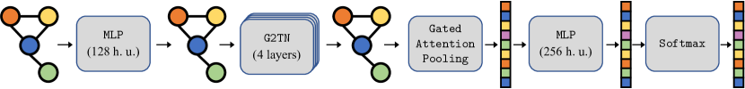
Figure 1: Visualization of the architecture used for NCI1 and NCI109 described in Section 5.

The architecture described in Section 5 is visualized conceptually on Figure 1, where for G2T(A)N the G2TN stack is replaced by the attentional variation without changing any hyperparameters. Further to the discussion given in the main text, here we provide more details on the model implementation.

Initialization.

In our G2TN and G2T(A)N layers, we linearly project tensor-valued features using linear functionals that use the same low-rank parametrization as the recursive variation in [toth_seq2tens_2020, App. D.2]. There, the authors also propose in Appendix D.5 an initialization heuristic for setting the variances of these component vectors, that we have employed with a centered uniform distribution.

Regularization.

We also apply $\ell_{2}$ regularization for both experiments in Sections 5 and H.3 for which we discuss the implementation here. Given a max. tensor degree $M\geq 1$ and a max. tensor rank $R\geq 1$ representing the layer width, there are overall $RM$ rank-$1$ linear functionals of the form

$${\boldsymbol{\ell}}^{r}_{m}=u^{r}_{M-m+1}\otimes\cdots\otimes u^{r}_{M}\quad\text{for }m=1,\dots M\text{ and }r=1,\dots,R.$$

Since in practice these are represented using only the component vectors $u^{r}_{i}\in\mathbb{R}^{d}$, a naive application of $\ell_{2}$ regularization would lead to computing the $2$-norm of each component vector $u^{r}_{i}$ to penalize the loss function. However, we found this approach to underperform compared to the following idea. Although our algorithm represents the functionals using a rank-$1$ decomposition and computes the projection of each tensor-valued node feature without explicitly building high-dimensional tensors, conceptually we still have tensors (${\boldsymbol{\ell}}_{m}^{r}$) acting on tensors ($\Phi(i)$ for $i\in\mathcal{V}$), and hence the tensor norm, $\left\lVert{\boldsymbol{\ell}}_{m}^{r}\right\rVert_{2}$, should be used for regularization. Fortunately, this can also be computed efficiently:

$$\left\lVert{\boldsymbol{\ell}}_{m}^{r}\right\rVert_{2}=\left\lVert u_{M-m+1}^{r}\otimes\cdots\otimes u_{M}^{r}\right\rVert_{2}=\left\lVert u_{M-m+1}^{r}\right\rVert_{2}\cdots\left\lVert u_{M}^{r}\right\rVert_{2}.$$

Further, as is common, we replace the $\ell_{2}$ norm with its squared value, sum over all functionals in (H.1), and multiply by the regularization parameter $\lambda>0$ so that the final penalty is given by

$$\texttt{L2Penalty}=\lambda\sum_{r=1}^{R}\sum_{m=1}^{M}\left\lVert u_{M-m+1}^{r}\right\rVert_{2}^{2}\cdots\left\lVert u_{M}^{r}\right\rVert_{2}^{2}.$$

H.2 Experiment Details.

Here we provide further details on the main experiment described in Section 5.

Hyperparameter Selection.

The model architecture was primarily motivated by GraphTrans (small) from [wu2021representing]. Specifically, the number and width of GNN layers, and the dropout rate was adopted as is. The $\ell_{2}$ regularization strength was chosen equal to the weight decay rate. The other hyperparameters were tuned on a single split of NCI1. For the random walk length, we experimented with values $2,5,10$. For the given GNN depth ($4$), $2$ RW steps per layer was not enough to learn long-range interactions, while $10$ significantly slowed down the convergence rate during training. For the maximal degree of tensors, we experimented with values from $2,3,4$, and using values beyond $2$ did not provide improvements. Intuitively, the tensor degree represents the order of nonlinear interactions that are learnable by the layer, e.g. a degree of $2$ encodes pairwise interactions between node features in the neighbourhood, while a higher degree of $M$ allows to encode interactions between certain $M$-tuples of nodes. We suggest that a degree of $2$ is a good baseline setting, and that increasing the GNN depth instead allows to efficiently capture higher order interactions, while increasing the effective influence radius at the same time. For the pre- and postprocessing layers, we experimented with various depths and choosing more than $1$ layer for each was counterproductive. The number of units was simply set to the GNN width ($128$) in the preprocessing layer, while for the postprocessing layer slightly increasing it was found to provide improvements ($256$), potentially to compensate for the large amount of information that is compressed in the pooling step.

Table 4: Accuracies computed over 5 seeds of G2TN ablated by changing a single option.

Dataset NoDiff NoZeroStart NoAlgOpt NoJK NoSkip NoNorm AvgPool NCI1 $79.1\pm 1.5$ $80.7\pm 0.6$ $78.9\pm 1.3$ $79.4\pm 1.9$ $81.0\pm 1.3$ $79.5\pm 1.1$ $80.3\pm 1.7$ NCI109 $77.8\pm 1.2$ $79.5\pm 1.5$ $76.5\pm 1.7$ $78.1\pm 1.9$ $77.0\pm 1.6$ $77.4\pm 2.7$ $77.6\pm 1.8$

Further Ablation Studies.

Here we extend the investigation of our model architectures that was partially given in Section 5 in Table 2. We give the analogous ablation study for the G2TN model in Table 4, and compare the derived conclusions between the attentional and attention-free versions. First, we discuss the layer variations. Similarly to G2T(A)N , NoDiff slightly decreases the accuracy. However the conclusions regarding NoZeroStart and NoAlgOpt are different. In this case, removing ZeroStart actually improves the performance, while on G2T(A)N the opposite was true. An interpretation of this phenomenon is that only the attention mapping that is used to learn the random walks required information about translations of the layer’s features, and not the tensor-features themselves. Another difference is that NoAlgOpt degrades the accuracy more significantly for G2TN . A possible explanation is that since G2T(A)N layers are more flexible thanks to their use of attention, they rely less on being able to learn the algebraic lift, while as G2TN layers are more rigid in their random walk definition, and benefit more from the added flexibility of AlgOpt. Additionally, it seems that G2TN is more sensitive to the various architectural options, and removing any of them, i.e. NoJK, NoSkip, NoNorm or AvgPool, degrades the accuracy by $1\%$ or more on at least one dataset. Intuitively, it seems that overall the G2T(A)N model is more robust to the various architectural “tricks”, and more adaptable due to its ability to learn the the random walk.

H.3 Further Experiments

Citation datasets.

Additionally to transductive learning on the biological datasets, we have carried out inductive learning tasks on some of the common citation datasets, i.e. Cora, Citeseer [sen2008collective] and Pubmed [namata2012query]. We follow [shchur2018pitfalls] in carrying out the experiment, and use the largest connected component for each dataset with $20$ training examples per class, $30$ validation examples per class, and the rest of the data used for testing. The hyperparameters of our models and optimization procedure were based on the settings of the GAT model in [shchur2018pitfalls, Table 4], which we have slightly fine-tuned on Cora and used for the other datasets. In particular, a single layer of G2TN or G2T(A)N is used with $64$ functionals, max. tensor degree $2$ and random walk length $5$. The dropout rate was tuned to $0.9$, while the attentional dropout was set to $0.3$ in G2T(A)N . Optimization is carried out with Adam [kingma2015adam], a fixed learning rate of $0.01$ and $\ell_{2}$ regularization strength $0.01$. Training is stopped once the validation loss does not improve for $50$ epochs, and restored to the best checkpoint. For both of our models, NoDiff is used that we found to improve on the results as opposed to using increments of node features. The dropout rate had to be tuned as high as $0.9$, which suggests very strong overfitting, hence the additional complexity of AlgOpt was also contrabeneficial, and NoAlgOpt was used. As such, each model employs a single hidden layer, which is followed by layer normalization that was found to perform slightly better than other normalizations, e.g. graph-level normalization.

Table 5: Accuracies of our models on the citation datasets computed over 100 seeds compared with the 4 consistently best performing baselines from [shchur2018pitfalls].

Dataset GCN GAT MoNet GraphSage (mean) G2TN (ours) G2T(A)N (ours) Cora $81.5\pm 1.3$ $81.8\pm 1.3$ $81.3\pm 1.3$ $79.2\pm 7.7$ $\mathbf{82.6\pm 1.0}$ $82.0\pm 1.1$ Citeseer $\mathbf{71.9\pm 1.9}$ $71.1\pm 1.9$ $71.2\pm 2.0$ $71.6\pm 1.9$ $69.4\pm 1.0$ $68.2\pm 1.3$ Pubmed $77.8\pm 2.9$ $78.7\pm 2.3$ $78.6\pm 2.3$ $77.4\pm 2.2$ $\mathbf{78.8\pm 1.9}$ $78.0\pm 1.9$

Table 6: Accuracies of our models on $k$-hop sanitized citation datasets computed over 100 seeds compared with the 5 consistently best performing models from [rampavsek2021hierarchical].

References

- [1] Pubchem. https://pubchem.ncbi.nlm.nih.gov/.
- [2] Uri Alon and Eran Yahav. On the bottleneck of graph neural networks and its practical implications. In International Conference on Learning Representations, 2021.
- [3] Jimmy Lei Ba, Jamie Ryan Kiros, and Geoffrey E Hinton. Layer normalization. arXiv preprint arXiv:1607.06450, 2016.
- [4] Dzmitry Bahdanau, Kyung Hyun Cho, and Yoshua Bengio. Neural machine translation by jointly learning to align and translate. In 3rd International Conference on Learning Representations, ICLR 2015, 2015.
- [5] Peter Battaglia, Razvan Pascanu, Matthew Lai, Danilo Jimenez Rezende, et al. Interaction networks for learning about objects, relations and physics. Advances in neural information processing systems, 29, 2016.
- [6] Patric Bonnier, Chong Liu, and Harald Oberhauser. Adapted topologies and higher rank signatures. arXiv preprint arXiv:2005.08897, 2020.
- [7] Karsten Borgwardt, Elisabetta Ghisu, Felipe Llinares-López, Leslie O’Bray, and Bastian Rieck. Graph kernels: State-of-the-art and future challenges. arXiv preprint arXiv:2011.03854, 2020.
- [8] Michael M. Bronstein, Joan Bruna, Taco Cohen, and Petar Veličković. Geometric Deep Learning: Grids, Groups, Graphs, Geodesics, and Gauges. arXiv:2104.13478 [cs, stat], May 2021.
- [9] Joan Bruna, Wojciech Zaremba, Arthur Szlam, and Yann LeCun. Spectral networks and locally connected networks on graphs. arXiv preprint arXiv:1312.6203, 2013.
- [10] J. Douglas Carroll and Jih-Jie Chang. Analysis of individual differences in multidimensional scaling via an n-way generalization of “Eckart-Young” decomposition. Psychometrika, 35(3):283–319, September 1970.
- [11] Benjamin Paul Chamberlain, James Rowbottom, Davide Eynard, Francesco Di Giovanni, Xiaowen Dong, and Michael M. Bronstein. Beltrami flow and neural diffusion on graphs. CoRR, abs/2110.09443, 2021.
- [12] Benjamin Paul Chamberlain, James Rowbottom, Maria I. Gorinova, Stefan D. Webb, Emanuele Rossi, and Michael M. Bronstein. GRAND: Graph Neural Diffusion. In The Symbiosis of Deep Learning and Differential Equations, September 2021.
- [13] Benjamin Paul Chamberlain, James R. Rowbottom, Maria I. Gorinova, Stefan Webb, Emanuele Rossi, and Michael M. Bronstein. Grand: Graph neural diffusion. In ICML, 2021.
- [14] Dexiong Chen, Laurent Jacob, and Julien Mairal. Convolutional kernel networks for graph-structured data. In International Conference on Machine Learning, pages 1576–1586. PMLR, 2020.
- [15] Zhengdao Chen, Soledad Villar, Lei Chen, and Joan Bruna. On the equivalence between graph isomorphism testing and function approximation with gnns. Advances in neural information processing systems, 32, 2019.
- [16] Ilya Chevyrev and Harald Oberhauser. Signature moments to characterize laws of stochastic processes. arXiv:1810.10971 [math, stat], 2018.
- [17] Thomas Cochrane, Peter Foster, Varun Chhabra, Maud Lemercier, Terry Lyons, and Cristopher Salvi. Sk-tree: a systematic malware detection algorithm on streaming trees via the signature kernel. In 2021 IEEE International Conference on Cyber Security and Resilience (CSR), pages 35–40. IEEE, 2021.
- [18] Michaël Defferrard, Xavier Bresson, and Pierre Vandergheynst. Convolutional neural networks on graphs with fast localized spectral filtering. Advances in neural information processing systems, 29, 2016.
- [19] Persi Diaconis. Group representations in probability and statistics. Lecture notes-monograph series, 11:i–192, 1988.
- [20] Ahmed A. A. Elhag, Gabriele Corso, Hannes Stärk, and Michael M. Bronstein. Graph anisotropic diffusion, 2022.
- [21] Federico Errica, Marco Podda, Davide Bacciu, and Alessio Micheli. A fair comparison of graph neural networks for graph classification. In International Conference on Learning Representations, 2019.
- [22] Michel Fliess. Fonctionnelles causales non linéaires et indéterminées non commutatives. Bulletin de la société mathématique de France, 109:3–40, 1981.
- [23] Bernard Gaveau. Principe de moindre action, propagation de la chaleur et estimees sous elliptiques sur certains groupes nilpotents. Acta Mathematica, 139(none):95–153, January 1977.
- [24] Justin Gilmer, Samuel S Schoenholz, Patrick F Riley, Oriol Vinyals, and George E Dahl. Neural message passing for quantum chemistry. In International conference on machine learning, pages 1263–1272. PMLR, 2017.
- [25] Daniele Grattarola and Cesare Alippi. Graph neural networks in tensorflow and keras with spektral [application notes]. IEEE Computational Intelligence Magazine, 16(1):99–106, 2021.
- [26] Alexander Grigoryan. Heat kernel and analysis on manifolds, volume 47. American Mathematical Soc., 2009.
- [27] Aditya Grover and Jure Leskovec. node2vec: Scalable feature learning for networks. In Proceedings of the 22nd ACM SIGKDD international conference on Knowledge discovery and data mining, pages 855–864, 2016.
- [28] Ben Hambly and Terry Lyons. Uniqueness for the signature of a path of bounded variation and the reduced path group. Ann. of Math., 171(1):109–167, 2010.
- [29] Will Hamilton, Zhitao Ying, and Jure Leskovec. Inductive representation learning on large graphs. Advances in neural information processing systems, 30, 2017.
- [30] Kaiming He, Xiangyu Zhang, Shaoqing Ren, and Jian Sun. Deep residual learning for image recognition. In Proceedings of the IEEE conference on computer vision and pattern recognition, pages 770–778, 2016.
- [31] Lars Hörmander. Hypoelliptic second order differential equations. Acta Mathematica, 119:147–171, 1967.
- [32] Diederik P Kingma and Jimmy Ba. Adam: A method for stochastic optimization. In ICLR, 2015.
- [33] Thomas Kipf and Max Welling. Semi-Supervised Classification with Graph Convolutional Networks. In International Conference on Learning Representations, 2017.
- [34] Franz J. Kiraly and Harald Oberhauser. Kernels for sequentially ordered data. J. Mach. Learn. Res., 20(31):1–45, 2019.
- [35] Johannes Klicpera, Stefan Weissenberger, and Stephan Günnemann. Diffusion improves graph learning. ArXiv, abs/1911.05485, 2019.
- [36] Risi Kondor. Diffusion kernels on graphs and other discrete structures. In ICML 2002, 2002.
- [37] Yann LeCun, Yoshua Bengio, et al. Convolutional networks for images, speech, and time series. The handbook of brain theory and neural networks, 3361(10):1995, 1995.
- [38] Yann LeCun, Léon Bottou, Yoshua Bengio, and Patrick Haffner. Gradient-based learning applied to document recognition. Proceedings of the IEEE, 86(11):2278–2324, 1998.
- [39] Darrick Lee and Robert Ghrist. Path Signatures on Lie Groups. arXiv:2007.06633 [cs, math, stat], 2020.
- [40] Junhyun Lee, Inyeop Lee, and Jaewoo Kang. Self-attention graph pooling. In International conference on machine learning, pages 3734–3743. PMLR, 2019.
- [41] Yujia Li, Richard Zemel, Marc Brockschmidt, and Daniel Tarlow. Gated graph sequence neural networks. In Proceedings of ICLR’16, 2016.
- [42] Ilya Loshchilov and Frank Hutter. Sgdr: Stochastic gradient descent with warm restarts. In ICLR, 2017.
- [43] Haggai Maron, Heli Ben-Hamu, Hadar Serviansky, and Yaron Lipman. Provably powerful graph networks. Advances in neural information processing systems, 32, 2019.
- [44] Ron Milo, Shai S. Shen-Orr, Shalev Itzkovitz, Nadav Kashtan, Dmitri B. Chklovskii, and Uri Alon. Network motifs: simple building blocks of complex networks. Science, 298 5594:824–7, 2002.
- [45] Federico Monti, Davide Boscaini, Jonathan Masci, Emanuele Rodola, Jan Svoboda, and Michael M Bronstein. Geometric deep learning on graphs and manifolds using mixture model cnns. In Proceedings of the IEEE conference on computer vision and pattern recognition, pages 5115–5124, 2017.
- [46] Christopher Morris, Martin Ritzert, Matthias Fey, William L. Hamilton, Jan Eric Lenssen, Gaurav Rattan, and Martin Grohe. Weisfeiler and Leman Go Neural: Higher-Order Graph Neural Networks. Proceedings of the AAAI Conference on Artificial Intelligence, 33(01):4602–4609, July 2019.
- [47] Galileo Namata, Ben London, Lise Getoor, Bert Huang, and U Edu. Query-driven active surveying for collective classification. In 10th International Workshop on Mining and Learning with Graphs, volume 8, page 1, 2012.
- [48] Giannis Nikolentzos and Michalis Vazirgiannis. Random walk graph neural networks. Advances in Neural Information Processing Systems, 33:16211–16222, 2020.
- [49] Bryan Perozzi, Rami Al-Rfou, and Steven Skiena. Deepwalk: Online learning of social representations. In Proceedings of the 20th ACM SIGKDD international conference on Knowledge discovery and data mining, pages 701–710, 2014.
- [50] Ladislav Rampášek and Guy Wolf. Hierarchical graph neural nets can capture long-range interactions. In 2021 IEEE 31st International Workshop on Machine Learning for Signal Processing (MLSP), pages 1–6. IEEE, 2021.
- [51] Linda Preiss Rothschild and Elias M. Stein. Hypoelliptic differential operators and nilpotent groups. Acta Mathematica, 137:247–320, 1976.
- [52] Franco Scarselli, Marco Gori, Ah Chung Tsoi, Markus Hagenbuchner, and Gabriele Monfardini. The graph neural network model. IEEE transactions on neural networks, 20(1):61–80, 2008.
- [53] Michael Schlichtkrull, Thomas N Kipf, Peter Bloem, Rianne van den Berg, Ivan Titov, and Max Welling. Modeling relational data with graph convolutional networks. In European semantic web conference, pages 593–607. Springer, 2018.
- [54] Alice C Schwarze and Mason A Porter. Motifs for processes on networks. SIAM Journal on Applied Dynamical Systems, 20(4):2516–2557, 2021.
- [55] Prithviraj Sen, Galileo Namata, Mustafa Bilgic, Lise Getoor, Brian Galligher, and Tina Eliassi-Rad. Collective classification in network data. AI magazine, 29(3):93–93, 2008.
- [56] Oleksandr Shchur, Maximilian Mumme, Aleksandar Bojchevski, and Stephan Günnemann. Pitfalls of graph neural network evaluation. arXiv preprint arXiv:1811.05868, 2018.
- [57] Nitish Srivastava, Geoffrey Hinton, Alex Krizhevsky, Ilya Sutskever, and Ruslan Salakhutdinov. Dropout: a simple way to prevent neural networks from overfitting. The journal of machine learning research, 15(1):1929–1958, 2014.
- [58] Robert S Strichartz. Sub-riemannian geometry. Journal of Differential Geometry, 24(2):221–263, 1986.
- [59] Matthew Thorpe, Tan Minh Nguyen, Hedi Xia, Thomas Strohmer, Andrea Bertozzi, Stanley Osher, and Bao Wang. GRAND++: Graph neural diffusion with a source term. In International Conference on Learning Representations, 2022.
- [60] Jake Topping, Francesco Di Giovanni, Benjamin Paul Chamberlain, Xiaowen Dong, and Michael M. Bronstein. Understanding over-squashing and bottlenecks on graphs via curvature, 2021.
- [61] Csaba Toth, Patric Bonnier, and Harald Oberhauser. Seq2Tens: An Efficient Representation of Sequences by Low-Rank Tensor Projections. In International Conference on Learning Representations, 2021.
- [62] N Th Varopoulos. Analysis and geometry on groups. Cambridge Tracts in Math., 100, 1992.
- [63] Ashish Vaswani, Noam Shazeer, Niki Parmar, Jakob Uszkoreit, Llion Jones, Aidan N Gomez, Łukasz Kaiser, and Illia Polosukhin. Attention is all you need. Advances in neural information processing systems, 30, 2017.
- [64] Petar Veličković, Guillem Cucurull, Arantxa Casanova, Adriana Romero, Pietro Liò, and Yoshua Bengio. Graph attention networks. In International Conference on Learning Representations, 2018.
- [65] Oriol Vinyals, Samy Bengio, and Manjunath Kudlur. Order matters: Sequence to sequence for sets. In ICLR, 2016.
- [66] Nikil Wale, Ian A. Watson, and George Karypis. Comparison of descriptor spaces for chemical compound retrieval and classification. Knowledge and Information Systems, 14(3):347–375, March 2008.
- [67] Wolfgang Woess. Random Walks on Infinite Graphs and Groups. Cambridge Tracts in Mathematics. Cambridge University Press, Cambridge, 2000.
- [68] Yuxin Wu and Kaiming He. Group normalization. In Proceedings of the European conference on computer vision (ECCV), pages 3–19, 2018.
- [69] Zhanghao Wu, Paras Jain, Matthew Wright, Azalia Mirhoseini, Joseph E Gonzalez, and Ion Stoica. Representing long-range context for graph neural networks with global attention. Advances in Neural Information Processing Systems, 34:13266–13279, 2021.
- [70] Louis-Pascal A. C. Xhonneux, Meng Qu, and Jian Tang. Continuous graph neural networks. In Proceedings of the 37th International Conference on Machine Learning, ICML’20, pages 10432–10441. JMLR.org, July 2020.
- [71] Keyulu Xu, Weihua Hu, Jure Leskovec, and Stefanie Jegelka. How powerful are graph neural networks? In International Conference on Learning Representations, 2019.
- [72] Keyulu Xu, Chengtao Li, Yonglong Tian, Tomohiro Sonobe, Ken-ichi Kawarabayashi, and Stefanie Jegelka. Representation learning on graphs with jumping knowledge networks. In International Conference on Machine Learning, pages 5453–5462. PMLR, 2018.
- [73] Rex Ying, Jiaxuan You, Christopher Morris, Xiang Ren, William L. Hamilton, and Jure Leskovec. Hierarchical graph representation learning with differentiable pooling. In Proceedings of the 32nd International Conference on Neural Information Processing Systems, NIPS’18, pages 4805–4815, Red Hook, NY, USA, December 2018. Curran Associates Inc.
- [74] Muhan Zhang, Zhicheng Cui, Marion Neumann, and Yixin Chen. An end-to-end deep learning architecture for graph classification. In Thirty-second AAAI conference on artificial intelligence, 2018.