Non-rigid Point Cloud Registration with
Neural Deformation Pyramid

Abstract

Non-rigid point cloud registration is a key component in many computer vision and computer graphics applications. The high complexity of the unknown non-rigid motion make this task a challenging problem. In this paper, we break down this problem via hierarchical motion decomposition. Our method called Neural Deformation Pyramid (NDP) represents non-rigid motion using a pyramid architecture. Each pyramid level, denoted by a Multi-Layer Perception (MLP), takes as input a sinusoidally encoded 3D point and outputs its motion increments from the previous level. The sinusoidal function starts with a low input frequency and gradually increases when the pyramid level goes down. This allows a multi-level rigid to non-rigid motion decomposition and also speeds up the solving by $50$ times compared to the existing MLP-based approach. Our method achieves advanced partial-to-partial non-rigid point cloud registration results on the 4DMatch/4DLoMatch benchmark under both no-learned and supervised settings. Code is available at https://github.com/rabbityl/DeformationPyramid.

Non-rigid point cloud registration is a key component in many computer vision and computer graphics applications. The goal of non-rigid registration is to find the transformation that maps one point cloud to another. With the availability of consumer range sensors that can measure time-varying surface points, non-rigid registration has been applied to dynamic shape reconstruction problems such as human performance capture, enabling a wide range of applications in XR and robotics.

Non-rigid registration is a challenging problem. First, 3D sensor measurements often contain noise, outliers, and occlusions. Occlusions often lead to disconnection of point cloud geometry. Point clouds may also have very low overlap ratios with each other due to the scene deformation and sensor’s viewpoint change. The most challenging thing is, unlike rigid registration that only needs to determine the rotation and translation parameters, non-rigid registration needs to estimate the unknown movement of all points, making this problem especially complex to solve.

In this paper, we alleviate this complexity through motion decomposition. We observe that natural non-rigid motion usually forms a hierarchical structure: with higher hierarchies representing the global movements and lower hierarchies representing the local deformation. For instance, a walking person can be roughly approximated by three levels: 1) global location and orientation change, 2) local articulated movements from arms, legs, etc, and 3) fine-grained cloth deformation caused by exterior forces. Each level represents motion at a different scale and they have top-down dependencies.

Based on this observation, we propose a hierarchical motion representation called Neural Deformation Pyramid (NDP) for non-rigid registration. NDP has a pyramid architecture. Each pyramid level contains a Multi-Layer Perception (MLP) that takes as input a sinusoidally encoded 3D point and outputs its motion increments from the previous level. We found that the frequency of the sinusoidal function controls MLP’s capacity of representing non-rigidity: low frequencies yield smooth signals that are suitable for fitting relatively rigid motion; high frequencies produce more fluctuations that are capable of representing highly non-rigid motion. We start the sinusoidal function at the first pyramid level with a low frequency and gradually increase it when the pyramid level goes down. This allows a multi-level rigid to non-rigid motion decomposition and also achieves over $50$ times faster solving than the existing MLP-based approach.

The paper is about developing an MLP-based hierarchical deformation model for non-rigid point cloud registration. The proposed method achieves state-of-the-art partial-to-partial non-rigid registration results on the challenging 4DMatch/4DLoMatch lepard2021 benchmark under both no-learned and supervised settings. We also demonstrate the application for shape transfer.

1 Related Work

Non-rigid point cloud registration.

Non-rigid point cloud registration is about estimating the deformation field or assigning point-to-point mapping from one point cloud to another. The simplest way is to estimate the point-wise parameters, such as affine transform, under motion smoothness regularization liao2009modeling . Optimal transport-based registration method geomloss finds displacement for each point using a global bijective-matching constraint. Coherent Point Drift (CPD) Coherent_point_drift ; bayesian_coherent_point_drift constructs a 3D displacement field using Gaussian Mixture Model (GMM) and encourages coherent motion of nearby points. Deformation graph embededdeformation represents the scene using a sparsely sub-sampled graph from the surface and propagates deformation from node to surface via “skinning”. The Non-rigid Iterative Closest Point (NICP) li2008regist achieve efficient registration by optimizing the alignment energy and deformation graph regularization cost arap , and has been adopted in many real-time 4D reconstruction systems dynamicfusion . Li et al. Learning2Optimize and Bozic et al. bovzivc2020neural learn dense feature alignment or correspondence re-weighting by differentiating through deformation graph-based non-rigid optimization. Learning-based scene flow estimation methods, e.g. FlowNet3D flownet , use 3D siamese networks to regress the 3D displacement field between two point clouds and reach real-time inference but are not robust under large deformations and ambiguities. Lepard lepard2021 use Transformer attention_is_all_u_need to learn global point-to-point mapping and use it as landmark to guide global non-rigid registration. Functional map approaches ovsjanikov2012functionalmaps estimate the correspondence in the spectral domain between computed Laplacian-Beltrami basis functions, but usually assume connected surfaces thus not suitable for real-world partial point cloud data. To alleviate this problem, Synorim huang2021SyNoRiM uses 3D CNN networks to estimate the basis functions and derive scene flow from the functional mapping. While existing methods mainly represent non-rigid motion or mapping at a single level, this paper propose a multi-level deformation model for non-rigid point cloud registration.

Pyramid for motion estimation.

Bouguet et al. lucas_kanade_pyramidal show that the pyramid implementation of the Lucas-Kanade cascade_lucas_kanade method improves feature tracking. PWCNet pwcnet estimates optical flow on a pyramid of CNN feature maps. PointPWC-net wu2019pointpwc adopts similar idea for scene flow estimation from point cloud inputs. Pyramid-based camera 6-Dof pose estimation can be found in SLAM systems lsdslam . ZoomOut melzi2019zoomout adopts upsampling in the spectral domain for shape correspondence estimation. DynamicFusion dynamicfusion constructs a tree of deformation graph for non-rigid tracking, and shows that it stabilizes tracking and reduces computation cost. DeepCap deepcap combines an inner body pose with an outer cloth deformation for human performance capture. This paper is about using MLP to create a hierarchical deformation pyramid for non-rigid point cloud registration of general scenes.

Motion field with coordinate-MLP.

Coordinate-MLP uses an MLP to map input coordinates to signal values. Coordinate-MLP is continuous and memory-efficient. It has shown promising results for representing 1D sound wave sitzmann2020siren , 2D images sitzmann2020siren , 3D shape occupancy_network , and radiance field mildenhall2020nerf , etc. Tancik et al. tancik2020fourier show that tuning the sinusoidal positional encoding of the input coordinate bias the network to fitting low- or high-frequency signals. Coordinate-MLP is also suitable for representing the deformation field. Close to our work, Li et al. li2021NSFF and Li et al. Neural_Scene_Flow_Prior use MLP to estimate scene flow, Nerfies park2021nerfies and SAPE hertz2021sape propose a coarse-to-fine motion field MLP optimization technique by progressively expanding the frequency bandwidth of the input positional encoding. However, the aforementioned motion field MLPs are black box models that are designed to represent signals at a single scale, and usually need a large network to fit complex motion, as a result their optimizations are usually time-consuming. This paper decomposes the motion field using a sequence of smaller MLPs, achieving more interpretable and controllable motion representation and faster optimization.

2 Non-rigid Point Cloud Registration Notation

Given a source point cloud $\mathbf{S}=\{{\mathbf{x}_{i}|\mathbf{x}_{i}\in\mathbb{R}^{3},{i=1,...,n_{1}}\}}$ and a target point cloud $\mathbf{T}=\{{\mathbf{y}_{j}|\mathbf{y}_{j}\in\mathbb{R}^{3},{j=1,...,n_{2}}\}}$, where $n_{1},n_{2}$ are the number of points, our goal is to recover the non-rigid warp function $\mathcal{W}:\mathbb{R}^{3}\mapsto\mathbb{R}^{3}$ that transforms points from $\mathbf{S}$ to $\mathbf{T}$. The simplest form of the warp function is a dense $\mathbb{R}^{3}$ vector field, which is also known as scene flow. Scene flow is in theory sufficient to represent any continuous deformation, but in practice, it can not fit non-linear motions very well, such as 3D rotations. We therefore formulate the non-rigid warp function using the $\operatorname{SE}(3)$ field.

Dense $\operatorname{SE}(3)$ warp field. Given a globally non-rigidly deforming point cloud, we consider each individual point locally undergoes 3D rigid body movement. A 3D rigid body transform $\scalebox{0.75}{\mbox{$\displaystyle\begin{pmatrix}\mathbf{R}&\mathbf{t}\\ 0&1\end{pmatrix}$}}\in\operatorname{SE}(3)$ denotes rotation and translation in 3D, with $\mathbf{R}\in\operatorname{SO}(3)$ and $\mathbf{t}\in\mathbb{R}^{3}$. We parameterize rotations with a 3-dimensional axis-angle vector $\boldsymbol{\omega}\in\mathbb{R}^{3}$. We use the exponential map $\exp:\mathfrak{so}(3)\rightarrow\operatorname{SO}(3),\quad\widehat{\boldsymbol{\omega}}\mapsto\mathrm{e}^{\widehat{\boldsymbol{\omega}}}=\mathbf{R}$ to convert from axis-angle to matrix rotation form, where the $\,\widehat{\cdot}$-operator creates a $3\times 3$ skew-symmetric matrix from a 3-dimensional vector. The resulting 3D motion parameterization for a point $\mathbf{x}_{i}\in\mathbb{R}^{3}$ is therefore denoted by $\boldsymbol{\xi}_{i}=\begin{pmatrix}\boldsymbol{\omega}_{i},\mathbf{t}_{i}\end{pmatrix}\in\mathbb{R}^{6}$, i.e. each point has 6 degrees of freedom (Dof). The warp function reads

$$\mathcal{W}(\mathbf{x}_{i},\boldsymbol{\xi}_{i})=\mathrm{e}^{\widehat{\boldsymbol{\omega}}_{i}}\mathbf{x}_{i}+\mathbf{t}_{i}$$ (1)

Dense $\operatorname{Sim}(3)$ warp field. This paper mainly focuses on registering point clouds captured from the same scene with the same scale. For scale variant tasks such as inter-shape registration (c.f. Sec. 4.3), we extend the above warp function by incorporating a scaling factor $s\in\mathbb{R}^{+}$, resulting in a 3D similarity transform $\scalebox{0.75}{\mbox{$\displaystyle\begin{pmatrix}s\mathbf{R}&\mathbf{t}\\ 0&1\end{pmatrix}$}}\in\operatorname{Sim}(3)$. With the parameterization $\boldsymbol{\xi}_{i}=\begin{pmatrix}s_{i},\boldsymbol{\omega}_{i},\mathbf{t}_{i}\end{pmatrix}\in\mathbb{R}^{7}$, the warp function reads $\mathcal{W}(\mathbf{x}_{i},\boldsymbol{\xi}_{i})=s_{i}\mathrm{e}^{\widehat{\boldsymbol{\omega}}_{i}}\mathbf{x}_{i}+\mathbf{t}_{i}$.

We shows ablation study of the dense warp field types including $\mathbb{R}^{3}$, $\operatorname{SE}(3)$, and $\operatorname{Sim}(3)$, and rotations representations including Axis-angle, Euler-angle, Quanterion, and 6D rotation_6D in Sec. 4.2.

3 Neural Deformation Pyramid

Figure 1: Neural Deformation Pyramid.

As denoted Sec. 2, we aim to find the motion parameter $\boldsymbol{\xi}_{i}$ for each 3D point $\mathbf{x}_{i}$ in the source point cloud. However, due to the high complexity and non-convexity of the non-rigid registration, directly estimating $\boldsymbol{\xi}_{i}$ is usually difficult and time-consuming. Therefore, we want to decompose $\boldsymbol{\xi}_{i}$ into a sequence of sub-transformations $\{\boldsymbol{\xi}_{i}^{1},\boldsymbol{\xi}_{i}^{2},...,\boldsymbol{\xi}_{i}^{m}\}$, such that each sub-transformation is easier to estimate, and when combining them we can get the same registration effect as $\boldsymbol{\xi}_{i}$.

To this end, we introduce Neural Deformation Pyramid (NDP) which allows hierarchical motion decomposition using a pyramid architecture.

3.1 Hierarchical motion decomposition.

As shown in Fig. 1, NDP is a pyramid of functions $\Delta=\{(\Gamma_{k},\Theta_{k})|{k=1,..,m}\}$, where each pyramid level contains a pair of continuous functions $(\Gamma_{k},\Theta_{k})$, and $m$ is the total number of levels.

At level $k$ of the pyramid, $\Gamma_{k}$ is the positional encoding function that maps the input point from previous level $\mathbf{x}_{i}^{k-1}\in\mathbb{R}^{3}$ using the sinusoidal encoding

$$\Gamma_{k}:\mathbb{R}^{3}\mapsto\mathbb{R}^{6},\quad\mathbf{x}_{i}^{k-1}\mapsto\Gamma_{k}(\mathbf{x}_{i}^{k-1})=(\text{sin}(2^{k+k_{0}}\mathbf{x}_{i}^{k-1}),\text{cos}(2^{k+k_{0}}\mathbf{x}_{i}^{k-1}))$$ (2)

where $k_{0}$ is a constant that controls the initial frequency at the first level of the pyramid. The frequency of the sinusoidal function is enssential for motion decomposition: low frequencies yield smooth signals that are suitable for fitting relatively rigid motion; high frequencies produce more fluctuations that are capable of representing highly non-rigid motion. By gradually increasing frequency with pyramid level $k$, we can achieve a hierarchical rigid-to-nonrigid motion decomposition. Fig. 2 shows an example of hierarchical registration of of multiple scans of a Dinosaur.

$\Theta_{k}$ is an optimizable MLP network. It takes as input the encoded coordinate $\Gamma_{k}(\mathbf{x}_{i}^{k-1})$ and estimates the transformation increments at the current pyramid level. Formally, we have

$$\Theta_{k}:\mathbb{R}^{6}\mapsto\mathbb{R}^{7},\quad\Gamma_{k}(\mathbf{x}_{i}^{k-1})\mapsto\Theta_{k}(\Gamma_{k}(\mathbf{x}_{i}^{k-1}))=(\boldsymbol{\xi}_{i}^{k},\alpha_{i}^{k})$$ (3)

where $\boldsymbol{\xi}_{i}^{k}\in\mathbb{R}^{6}$ is the 6-Dof transformation parameter that is obtained from a liner output head of the MLP. $\alpha_{i}^{k}\in[0,1]$ is a scalar that represents the network’s confidence in if the motion estimates are successful at the current level, it is obtained via a Sigmoid output head of the MLP.

Given the 6-Dof estimates $\boldsymbol{\xi}_{i}^{k}$ and confidence $\alpha_{i}^{k}$, we compose the transformed coordinate at the $k$-th level by

$$\mathbf{x}_{i}^{k}\leftarrow\mathbf{x}_{i}^{k-1}+\alpha_{i}^{k}\cdot\mathcal{W}(\mathbf{x}_{i}^{k-1},\boldsymbol{\xi}_{i}^{k})$$ (4)

where $\mathcal{W}$ is the warp function as defined in Eqn. 1. Note that $\alpha_{i}^{k}$ control the degree of deviation w.r.t to the previous more rigid pyramid level, thus we regard it as the level-wise deformability. To encourage as-rigid-as-possible movement, we apply regularization terms on $\alpha_{i}^{k}$ which is shown in the next.

Merits of hierarchical motion decomposition. 1) it provides a more controllable and interpretable coordinate MLP-based deformation representation. 2) it simplifies the task and speedup the optimization: we can use a small MLP for each level, because each level only needs to estimate the motion increments at a single frequency band, we also found that the overall convergence of the pyramid is faster than using a single coordinate-MLP with the full frequency band, this significantly cut off the total optimization time compared to the existing MLP-based approaches, c.f. discussion in Sec. 4.2.

Figure 2: Hierarchical non-rigid registration of multiple scans of a Dinosaur using LNDP. We show the outputs from the 1st, 4th, and 8th level of the deformation pyramid. The pink color denotes the target point cloud, the rests are the sources (the figures in this paper are best viewed on screen).

3.2 Cost function.

At level $k$, we denote the transformed source point cloud as $\mathbf{S}^{k}=\{\mathbf{x}_{i}^{k}|{i=1,...,n_{1}}\}$. The target point cloud is $\mathbf{T}=\{{\mathbf{y}_{j}|{j=1,...,n_{2}}\}}$. The cost functions at level $k$ are:

Chamfer distance term. Chamfer distance finds the nearest point in the other point cloud, and sums the square of distance. Formally it is defined as

$$E^{k}_{cd}=\frac{1}{|\mathbf{S}^{k}|}\sum_{\mathbf{x}_{i}^{k}\in\mathbf{S}^{k}}\min_{\mathbf{y}_{j}\in\mathbf{T}}\rho(\mathbf{x}_{i}^{k}-\mathbf{y}_{j})+\frac{1}{|\mathbf{T}|}\sum_{\mathbf{y}_{j}\in\mathbf{T}}\min_{\mathbf{x}_{i}^{k}\in\mathbf{S}^{k}}\rho(\mathbf{x}_{i}^{k}-\mathbf{y}_{j})$$ (5)

where $\rho(.,.)$ is the distance function, for which we use $L_{1}$ or $L_{2}$ norm. We found that the robust $L_{1}$ norm is more suitable for handling partial-to-partial registration, see ablation study in Section. 4.

Correspondence term. Given a putative correspondence set $\mathcal{M}$, we minimize

$$E^{k}_{cor}=\frac{1}{|\mathcal{M}|}\sum_{(u,v)\in\mathcal{M}}\rho(\mathbf{x}_{u}^{k}-\mathbf{y}_{v})$$ (6)

where $(u,v)\in\mathcal{M}$ are the indices of the matched points in $\mathbf{S}^{k}$ and $\mathbf{T}$. To obtain correspondence, we leverage the learning-based point cloud matching method Lepard lepard2021 , which predicts sparse point-to-point matches. Lepard’s prediction contains a certain amount of outlier correspondences, which may lead to erroneous registration. To alleviate this, we design a Transformer-based outlier rejection method, which takes as input matched coordinates pairs $(u,v)\in\mathbb{R}^{6}$ and estimates their outlier probabilities. The details can be seen in the supplemental material.

Deformability regularization term. Given the deformability score $\alpha_{i}^{k}$ in Eqn. 4, we encourages zero predictions by minimizing the negative log-likelihood

$$E^{k}_{reg}=\frac{1}{|\mathbf{S}^{k}|}\sum_{\mathbf{x}_{i}\in\mathbf{S}^{k}}-\log(1-\alpha_{i}^{k})$$ (7)

This is to encourage as-rigid-as-possible movement. We found this regularization help preserve the geometry of the point cloud given high frequency input signals.

Total cost function. The total cost function $E^{k}_{total}$ combines the above terms with the weighting factors $\lambda_{cd}$, $\lambda_{cor}$, and $\lambda_{reg}$ to balance them :

$$E^{k}_{total}=\lambda_{cd}E^{k}_{cd}+\lambda_{cor}E^{k}_{cor}+\lambda_{reg}E^{k}_{reg}$$ (8)

In the case that we use the correspondence term $E_{cor}$, we denote our method as LNDP where ‘L’ indicates the Learned correspondences.

3.3 Non-rigid registration algorithm

Non-rigid registration using NDP is performed in a top-down way: the top-level MLP is firstly optimized, once it converges, proceeds to a lower level, we repeat this till all MLPs are optimized. We use gradient descent as the optimizer. Optimization of an MLP stops if 1) the $max\_iter=500$ is reached, 2) a given registration cost threshold $\gamma=0.0001$ is reached, or 3) the registration cost does not change for more than $\sigma=15$ iterations. Alg. 1 shows the pseudocode of the algorithm.

Algorithm 1 Non-rigid registration using NDP

1:function  Registration($\mathbf{S}^{0},\mathbf{T}$) $\triangleright$ $\mathbf{S}^{0}$ denotes the raw source point cloud

2:     for $k\leftarrow 1$ to $m$ do

3:         $\Theta_{k}\leftarrow\mathrm{XavierUniform()}$ $\triangleright$ MLP initialization

4:         for $iter\leftarrow 1$ to $max\_iter$ do

5:              $\mathbf{S}^{k}\leftarrow\mathrm{TransformSourcePointCloud}(\mathbf{S}^{k-1},\Gamma_{k},\Theta_{k})$

6:              $E^{k}_{total}\leftarrow\mathrm{ComputeRegistrationCost}(\mathbf{S}^{k},\mathbf{T})$

7:              if  $\mathrm{ConvergenceConditionSatisfied}(E^{k}_{total},iter)$  then $\triangleright$ Early stop

8:                  break               

9:              $\Theta_{k}\leftarrow\mathrm{GradientDecentSolver}(\Theta_{k},E^{k}_{total})$ $\triangleright$ Update MLP weights               

10:     return $\mathbf{S}^{m}$

Figure 3: Quantitative non-rigid registration results for the Dragon. For each method, we show the point cloud alignment and error map. Sinkhorn does not preserve the point cloud topology. CPD and NICP can easily fall into local minima. The scene flow produced by PointPWC and Synonym-pw distorts the geometry. Synonym-pw does not generalize well to uncommon shapes in the dataset such as this dragon.

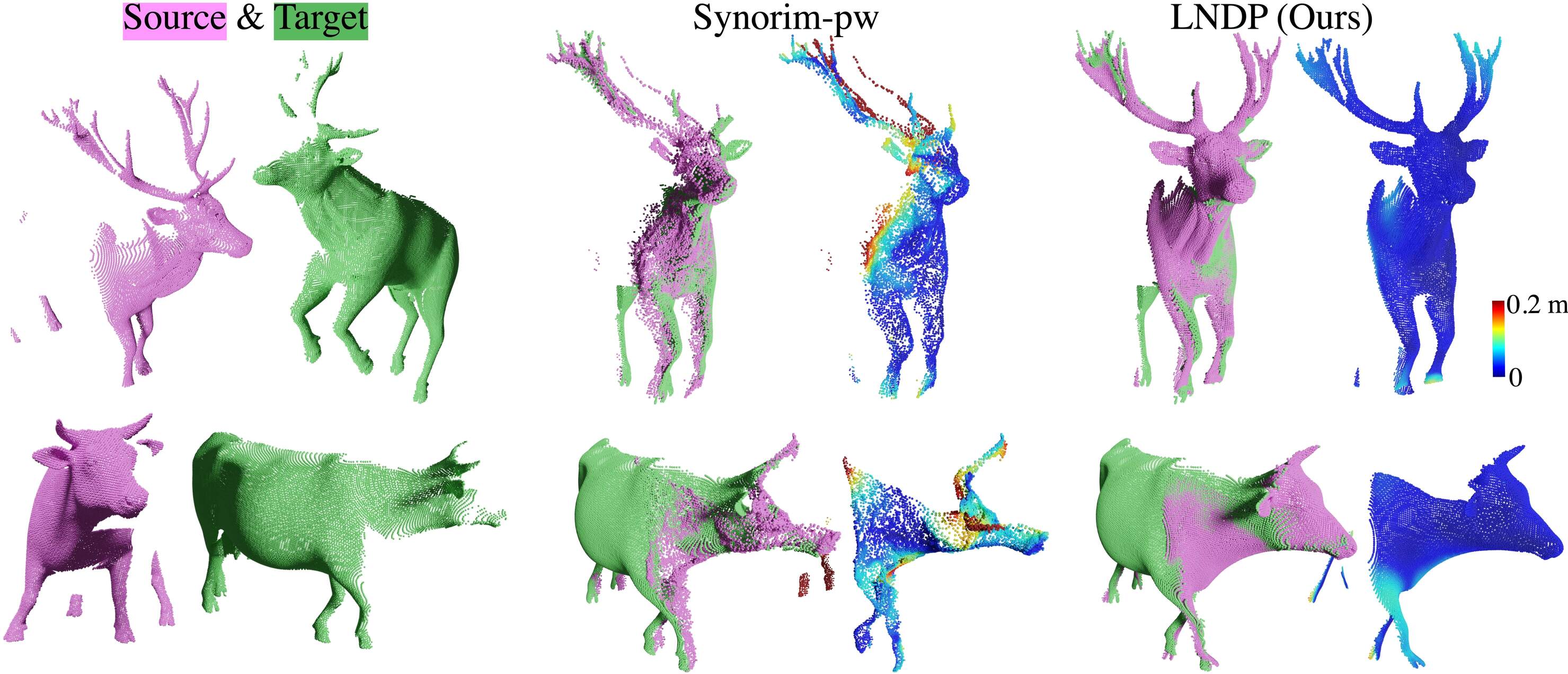
Figure 4: Quantitative non-rigid registration results for the Deer and Cow. Synorim-pw runs on subsampled 8192 points. LNDP can directly warp all input points because it is a continuous function. LNDP better preserves the geometry, especially for the non-overlapping regions.

4 Experiments

4.1 Benchmarking partial-to-partial non-rigid point cloud registration

4DMatch/4DLoMatch benchamrk. 4DMatch/4DLoMatch lepard2021 is a benchmark for non-rigid point cloud registration. It is constructed using animation sequences from DeformingThings4D li20214dcomplete . This benchmark is extremely challenging due to the partial overlap, occlusions, and large motion present in the data. Point cloud pairs in this benchmark have a wide range of overlap ratios: $45\%-92\%$ in 4DMatch and $15\%-45\%$ in 4DLoMatch. We found that the original benchmark contains a certain amount of examples that are dominated by rigid movement. For fair evaluation, we remove data with near-rigid movements, please check the supplementary for details.

Table 1: Quantitative non-rigid registration results on 4DMatch and 4DLoMatch.

		4DMatch				4DLoMatch
	Method	EPE$\downarrow$	AccS $\uparrow$	AccR $\uparrow$	Outlier$\downarrow$	EPE$\downarrow$	AccS$\uparrow$	AccR$\uparrow$	Outlier$\downarrow$	Time $\downarrow$
No-Learned	ICP ICP-besl1992 †	0.296	2.96	12.06	71.50	0.565	0.14	0.74	90.87	0.10
	ZoomOut melzi2019zoomout	0.598	1.82	4.23	89.27	0.663	0.22	0.81	90.39	151.10
	CPD Coherent_point_drift	0.274	1.57	7.30	74.52	0.463	0.07	0.48	84.49	4.52
	BCPD bayesian_coherent_point_drift	0.291	5.13	12.35	73.74	0.492	0.20	0.86	86.88	5.81
	Sinkhorn geomloss	0.308	2.76	8.13	79.86	0.505	0.20	0.81	89.47	3.76
	NICP dynamicfusion	0.325	6.44	12.10	80.04	0.517	0.18	0.73	92.37	4.80 ‡
	NSFP Neural_Scene_Flow_Prior	0.265	8.66	18.65	64.96	0.495	0.38	1.56	84.77	39.54 ‡
	Nerfies park2021nerfies	0.280	12.65	25.41	58.91	0.498	1.05	3.01	82.21	115.94 ‡
	NDP (Ours)	0.195	18.69	35.64	45.04	0.467	0.79	3.05	80.47	2.31 ‡
Supervised	Lepard lepard2021 +SVD†	0.137	6.91	24.50	43.43	0.160	5.27	19.77	44.16	0.06 ‡
	PointPWC wu2019pointpwc	0.182	6.25	21.49	52.07	0.279	1.69	8.15	55.70	0.06 ‡
	FLOT puy2020flot	0.133	7.66	27.15	40.49	0.210	2.73	13.08	42.51	0.07 ‡
	GeomFmaps deepgeofm2020	0.152	12.34	32.56	37.90	0.148	1.85	6.51	64.63	135.18
	Synorim-pw huang2021SyNoRiM	0.099	22.91	49.86	26.01	0.170	10.55	30.17	31.12	0.41‡
	Lepard+NICP lepard2021	0.097	51.93	65.32	23.02	0.283	16.80	26.39	52.99	3.93 ‡
	LNDP (Ours)	0.075	62.85	75.26	16.78	0.169	28.65	43.37	32.14	2.39 ‡

• ${\dagger}$ rigid registration methods.   ${\ddagger}$ with GPU accerleration (NVIDIA A100).

Metrics. The metrics for evaluating non-rigid registration quality are 1) End-Point Error (EPE), i.e., the average norm of the 3D warp error vectors over all points, 2) 3D Accuracy Strict (AccS), the percentage of points whose relative error < 2.5% or < 2.5 cm, 3) 3D Accuracy Relaxed (AccR), the percentage of points whose relative error < 5% or < 5 cm, and 4) Outlier Ratio, the percentage of points whose relative error > 30%. We consider AccS and AccR as the most important metrics as they exactly measure the ratio of accurately registered points.

Baselines.

We benchmark non-rigid registration using a number of baselines under both the no-learned and supervised settings. We use the underlined names for brevity:

• No-Learned. Point-to-point Iterative Closest Point (ICP) ICP-besl1992 implemented in Open3D Open3D , Coherent Point Drift (CPD)Coherent_point_drift and its Bayesian formulation BCPD bayesian_coherent_point_drift , ZoomOut melzi2019zoomout , Sinkhorn optimal transport method implemented in Geomloss geomloss and Keops feydy2020keops , point-to-point Non-rigid ICP (NICP) dynamicfusion , coordinate-MLP based approaches including Neural Scene Flow Prior (NSFP) Neural_Scene_Flow_Prior and Nerfies park2021nerfies .

• Supervised. Procrustes approach using Lepard lepard2021 ’s feature matching followed by SVD solver arun1987procrustes (Lepard+SVD), Deep Geometric Maps (GeomFmaps) donati2020deepGeoMaps , Synorim huang2021SyNoRiM in the pair-wise setting (Synorim-pw), scene flow estimation methods including FLOT puy2020flot and PointPWC wu2019pointpwc , feature matching enhanced NICP as in lepard2021 (Lepard+NICP). All supervised models are re-trained on 4DMatch’s training split before evaluation.

Benchmarking results. Tab. 1 shows the quantitative non-rigid registration results. The coordinate-MLP-based methods, including NSFP, Nerfies, and our NDP get clearly better results than other no-learned baselines. This indicates the advantages of using the continuous coordinate-MLP to represent motion. A major drawback of Nerfies and NSFP is that their optimization is usually time-consuming. With hierarchical motion decomposition, our NDP runs around $50$ times faster than Nerfies and still be equally or more accurate. Note that on 4DMatch, NDP even outperforms the supervised methods FLOT and PointPWC on the AccS/AccR metrics by a significant margin. On 4DLoMatch, due to the small point cloud overlap ($15\%-45\%$), none of the no-learned methods can produce a reasonable result. LNDP obtains significantly better non-rigid registration results than other supervised baselines. Fig. 2,  3, and  4 shows the qualitative non-rigid registration results.

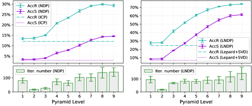
Figure 5: Point cloud registration accuracies (top) and gradient descent iterations (bottom) at each pyramid level on the 4DMatch benchmark. Left: NDP, right: LNDP.

Table 2: Ablation study of loss functions.

	4DMatch				4DLoMatch
Method	EPE$\downarrow$	AccS $\uparrow$	AccR $\uparrow$	Outlier$\downarrow$	EPE$\downarrow$	AccS$\uparrow$	AccR$\uparrow$	Outlier$\downarrow$
NDP ($L_{2}$ Chamfer distance term )	0.205	14.34	29.79	48.4	0.473	0.82	3.03	80.92
NDP ($L_{1}$ Chamfer distance term )	0.195	18.69	35.64	45.04	0.467	0.79	3.05	80.47
LNDP ($L_{2}$ Correspondence term )	0.078	61.27	74.10	17.50	0.177	26.59	41.50	33.81
LNDP ($L_{1}$ Correspondence term )	0.075	62.85	75.26	16.78	0.169	28.65	43.37	32.14

Table 3: Ablation study of warp field type and rotation representation in LNDP.

		4DMatch				4DLoMatch
Warp field	Rotation format	EPE$\downarrow$	AccS$\uparrow$	AccR$\uparrow$	Outliers$\downarrow$	EPE$\downarrow$	AccS$\uparrow$	AccR$\uparrow$	Outliers$\downarrow$	Iter.$\downarrow$
$\mathbb{R}^{3}$	–	0.084	58.03	70.91	19.15	0.197	21.46	34.30	40.00	882
$\operatorname{SE}(3)$	6D rotation_6D	0.080	56.15	72.04	18.71	0.172	26.95	43.09	32.14	1077
	Quaternion	0.080	55.47	71.87	18.73	0.168	26.79	43.29	31.33	1010
	Euler angle	0.075	62.72	75.21	16.80	0.169	28.89	43.68	32.17	799
	Axis-angle (Default)	0.075	62.85	75.26	16.78	0.169	28.65	43.37	32.14	785
$\operatorname{Sim}(3)$	Axis-angle	0.079	59.33	72.35	19.86	0.173	24.74	42.56	33.01	1388

4.2 Ablation study

Pyramid level. We test 9 pyramid levels with the initial frequency parameters in Eqn. 2 set to $k_{0}=-8$. Fig. 5 shows that, 1) the first level only slightly surpasses the rigid registration baseline, 2) the registration accuracies gradually increase with the pyramid level, i.e., the capacity of representing non-rigid motion gradually grows, and 3) lower levels tend to need more iterations to converge.

Why is NDP faster than Nerfies? Summing up the iterations from all levels (c.f. Fig. 5), NDP needs a total of 738 gradient decent iterations to converge. The coarse-to-fine optimization in Nerfies uses a single MLP with the full frequency band as input. As a comparison, Nerfies needs 3792 iterations for convergence. This indicates that our motion decomposition method speeds up the overall convergence. In addition, to represent complex motions, Nerfies needs a large MLP of $(\text{witdth, depth})=(128,7)$. As a comparison, for each pyramid level we use a small MLP of $(\text{witdth, depth})=(128,3)$, because each level only needs to estimate the motion increments at a single frequency band. Note that NDP only queries a single level MLP at an iteration (c.f. Algorihtm. 1). As a result, the overall computation overhead of NDP is much smaller than Nerfies.

L${}_{\text{1}}$ norm vs L${}_{\text{2}}$ norm for partial registration. We show in Table. 2 that the $L_{1}$ norm is more suitable for partial-to-partial registration, because it is more robust to large errors. For example, the chamber distance term is based on the sum of the squared distance from each point to the other model. Minimizing this loss would attempt to reduce the distance for every point, including those that do not correspond to any point on the other point cloud due to the partial overlap. Compared to the $L_{2}$ norm, the $L_{1}$ norm allow for large distances on some points. Similarly, the $L_{1}$ norm is also more tolerant to outliers in the correspondence term.

Motion field type. Tab. 3 shows that, 1) $\operatorname{SE}(3)$ warp field gets better results than $\operatorname{Sim}(3)$ field and $\mathbb{R}^{3}$ vector field, and 2) $\operatorname{Sim}(3)$ field requires the most iterations to converge, possibly because it needs to estimate the extra scale factor.

Rotation representation. Tab. 3 shows that Axis-angle and Euler angle get similar results and are better and converge faster than Quanterion and 6D.

4.3 Scale variant registration with Sim(3) warp field

In Fig. 6, we provide examples of the “shape transfer” as an application of our non-rigid registration method. To handle scale change between different shapes, we employ the dense $\operatorname{Sim}(3)$ warp field (c.f. Sec. 2). The dense formulation allows NDP to reflect different scale changes at different regions of the body, e.g. character $\mathbf{A}$’s stomach is expanding while the legs are shrinking. The original mesh vertices of the shapes are unevenly distributed, which is not suitable for computing the chamfer distance cost as in Eqn. 5, therefore we use uniformly sub-sampled point clouds from the mesh’s surface as input points. Since NDP is a continuous function, the deformed mesh can be obtained by querying NDP using the original mesh’s vertices. We use the registration parameters $(m,k_{0})=(9,-8)$, this allows the transformed shapes roughly match the target shapes while retaining the geometrical details of the source shapes.

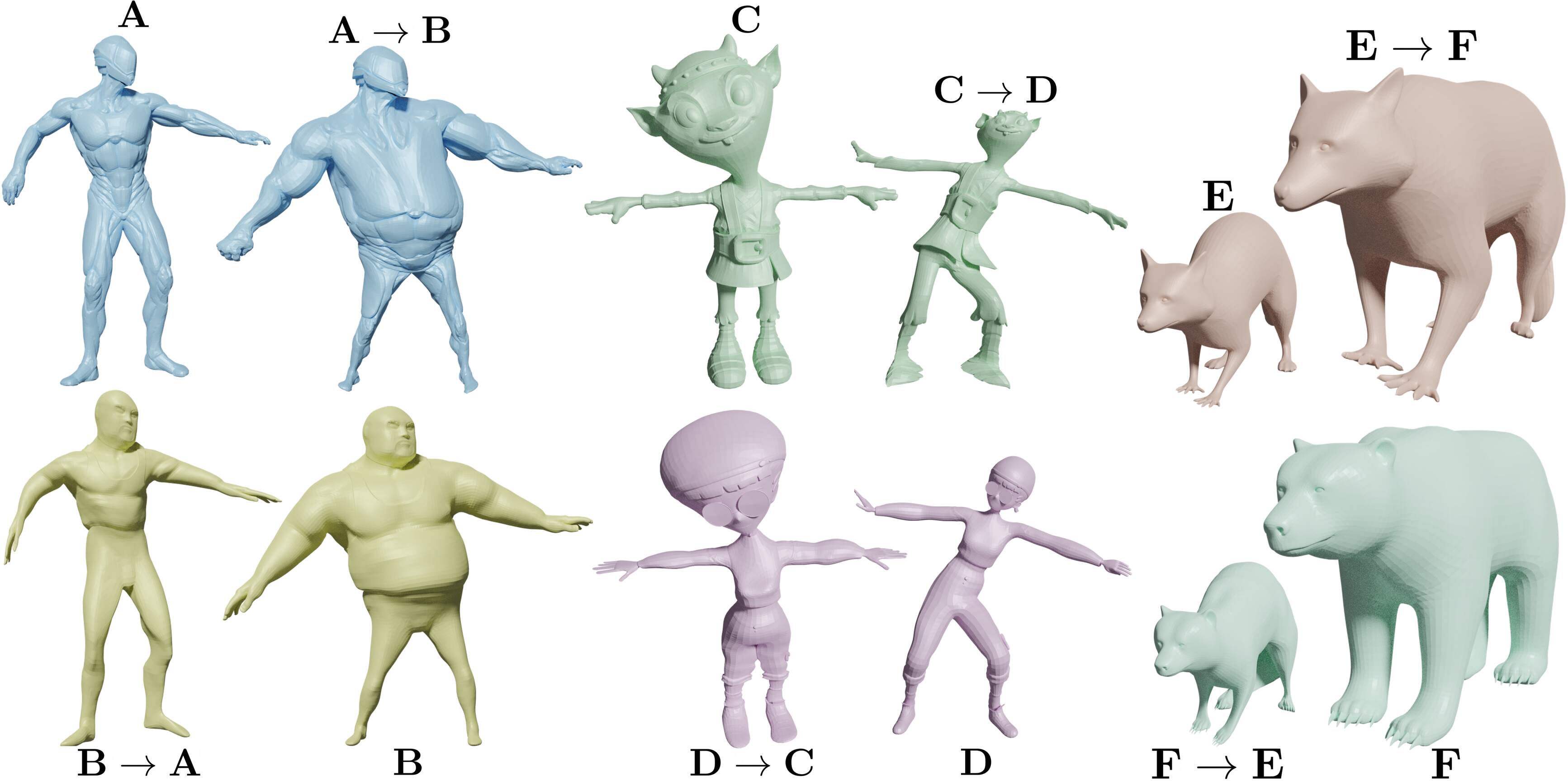
Figure 6: Shape transfer using NDP. The input shapes $\mathbf{A}$, $\mathbf{B}$, $\mathbf{C}$, and $\mathbf{D}$ are “Alien Soldier”, “Ortiz”, “Doozy”, and “Jackie” from Mixamo (https://www.mixamo.com/); $\mathbf{E}$ and $\mathbf{F}$ are “Racoon” and “Bear” from DeformingThings4D li20214dcomplete . The arrows indicate the directions of transfer.

5 Conclusion

We show that non-rigid point cloud registration can be decomposed into a hierarchical motion estimation schema by stacking coordinate networks with growing input frequency. Our method demonstrates superior non-rigid registration results on the 4DMatch partial-to-partial non-rigid registration benchmark under both no-learned and supervised settings. Our method runs over $50$ times faster than the existing coordinate-networks-based approach.

Limitations.

1) NDP uses input coordinates that are defined over the 3D Euclidean space, therefore it can not handle topological changes very well, extending NDP to the manifold surface space would be interesting. 2) Common to the unsupervised approach, NDP does not handle non-isometric cases. A failure case could be seen in Figure. 6: i.e. A’s chest is mapped to B’s belly. 3) Though NDP runs about $50$ times faster than Nerfies, the current implementation still does not run at a real-time rate, further speedup could leverage the tiny CUDA neural network framework tiny-cuda-nn . 4) Finally, non-rigid registration in the low-overlap cases, such as examples in 4DLoMatch, is still challenging, our method cannot solve all the cases.

Broader Impact.

Our paper presents non-rigid registration, which is needed for a variety of applications ranging from XR to robotics. In the former, a precise modeling of dynamic and deformable objects is of major importance to provide an immersive experience to the user. In the later, localizing and understanding dynamic objects such as humans and animals in the envoriment using 3D sensor is essential for safe and intellegent robot operation. On the other hand, as a low-level building block, our work has no direct negative outcome, other than what could arise from the aforementioned applications.

Supplementary Material:
Non-rigid Point Cloud Registration with Neural Deformation Pyramid

I. Introduction

Supplemental document includes

• Additional ablation studies, see. II..

• Results on real-world benchmarks: DeepDeform and KITTI, see III.

• Details of our outlier rejection approach, see. IV..

• Details of data filter in 4DMatch benchmark, see V..

II. Ablation Study

Ablation study of the network weights initialization.

Changing the initialization strategy could greatly affects the results of registration. Table. I shows an ablation study for network initialization via Pytorch built-in functions. With .ones_ initialization, the model does not converge at all. .kaiming_uniform_ and .xavier_uniform_ initialization produce similar results.

Table I: Ablation study of Pytorch init functions for NDP on 4DMatch.

torch.nn.init	EPE(cm)	AccS(%)	AccR(%)	Outlier(%)
.ones_	47706.20	0.00	0.00	100.00
.zeros_	21.83	3.48	13.89	60.00
.kaiming_uniform_	20.89	14.93	29.81	50.34
.xavier_uniform_ (Default)	20.05	14.34	29.79	48.4

In addition, we employ a trick to constraint the output of MLP: we apply a small scaling factor of $0.0001$ on the output of MLP, this encourages the MLP to produce a near-identity $SE(3)$ matrix at the beginning of optimization. We found this trick is crucial for NDP (no-learned) but not necessary for LNDP (supervised).

Computation time at a different number of input points.

The time complexity of our registration algorithm is sub-linear or $\mathcal{O}(1)$ with the number of points. The dominant computation overhead is from the network optimization, the time complexity is $\mathcal{O}(n\times m)$, where $n$ is the number of points and $m$ is the number of iterations required for convergence. If $m$ is fixed, the time grows in of the number of points. However, we found that when increasing training point $n$, the total number of iteration $m$ decreases. Therefore, if we use all points for optimization, the registration time grows sub-linearly. For faster registration, we can optimize only sub-sampled points. This keeps a constant registration time regardless of the input size. Table. II proves this argument.

Table II: Registration time (s) of NDP at different number of input points.

Complexity		2k	4k	6k	8k	10k	12k	14k	16k	18k	20k
$\mathcal{O}(n)$		2.72	5.42	8.13	10.84	13.55	16.25	18.97	21.68	24.39	27.1
sub-linear	(w/ all points)	2.72	3.56	3.79	3.78	4.84	5.06	5.07	5.7	6.38	5.91
$\mathcal{O}(1)$	(w/ sampled 2k points)	2.72	2.58	2.6	2.57	2.47	2.82	2.63	2.76	2.58	2.87

Registration result at different level of noise.

Table. III shows the registration accuracy of NDP under different ratios of point cloud noise. A noisy point is created via uniform perturbation of a clean point inside a ball with a radius=0.5m (the size of objects in 4DMatch range from 0.6m to 2.1m). We do not observe a significant performance drop until the introduction of $25\%$ noise, while real-world range sensors such as the Kinect1 camera only produces $4\%$-$6\%$ noise, see [27]. This experiment, combined with the results on DeepDeform and KITTI, proves that our method is robust to noisy data in real-world scenarios.

Table III: Registration Accuracy Relaxed (AccR) of NDP on 4DMatch under different level of noise.

Noise ratio	0%	5%	10%	15%	20%	25%	30%	35%	40%	45%	50%
AccR (%)	29.81	28.76	27.74	27.08	27	24.43	24.25	24.22	23.89	22.64	21.83

Experiment with different level of Overlap/Partiality/Occlusion.

We want to clarify that, in the pair wise setting, the three terms: overlap, partiality, and occlusion are connected. Given $\text{Overlap ratio}=\theta$, we can obtain the others by $\text{Partiality}=\theta$ , and $\text{Occlusion Ratio}=(1-\theta)$. Because overlap ratio is defined by the the percentage of co-visible point between a pair of point clouds, by this definition, overlap ratio exactly represents the relative partiality between two point clouds. Occlusion ratio denotes the ratio of points that are invisible from another point cloud, therefore it is can be computed by $(1-\theta)$. Table. II. shows the stats of in 4DMatch/4DLoMatch. Note that our method is state-of-the-art on this benchmark, c.f. Table. 1.

	Overlap ratio / Partiality ( $\theta$ )	Occlusion ratio ($1-\theta$)
4DMatch	45%$\sim$92%	8%$\sim$55%
4DLoMatch	15%$\sim$45%	55%$\sim$85%

As shown in Table. IV, we further re-group the results on 4DMatch/4DLoMatch based on different ranges of with 20% interval.

Table IV: Registration Accuracy (AccR) at different level of overlap ratio.

Overlap ratio ($\theta$)	<20%	20% $\sim$40%	40% $\sim$60%	60% $\sim$80%	>80%
AccR (%) with NDP	0.97	2.8	8.16	25.57	63.65
AccR (%) with LNDP	19.01	39.32	63.37	71.91	89.77

III. Results on DeepDeform [6] and KITTI [15] benchmark

We report results on two real-world benchmarks: DeepDeform [6], and KITTI Scene Flow [15]. DeepDeform contains real-world partial RGB-D scans of dynamic objects, including humans, animals, cloth, etc. KITTI Scene Flow dataset contains Lidar scans in dynamic autonomous driving scenes.

Table. VI and V shows the quantitative registration results and Figure. I and II show the qualitative results. Our NDP produces advanced results on both benchmarks. In particular, the Lidar scans in KITTI capture running vehicles, walking pedestrians, and static trees/buildings on the road, i.e., the data is cluttered, and breaks the isometric deformation assumption. The point density of Lidar scans also changes drastically from near to far. NDP is robust to the above factors and produces competitive results.

Table V: Registration results on KITTI Scene Flow benchmark.

	Supervised	EPE(m)	AccS(%)	AccR(%)
FlowNet3D [8]	Yes	0.199	10.44	38.89
PointPWC [38]	Yes	0.142	29.91	59.83
NDP (Ours)	No	0.141	47.00	71.2

Table VI: Registration results of no-learned methods on DeepDeform benchmark.

	EPE(cm)	AccS(%)	AccR(%)	Outlier(%)
ZoomOut [23]	2.88	62.31	85.74	19.55
Sinkhorn [11]	4.08	42.49	77.41	23.85
NICP [28]	3.66	48.16	80.16	21.34
Nerfies [30]	2.97	61.58	86.82	16.11
NDP (Ours)	2.13	79.01	94.09	11.55

Figure I: Qualitative non-rigid registration results of NDP on DeepDeform benchmark. From the left to right are the initial point cloud alignment and the registered point cloud.

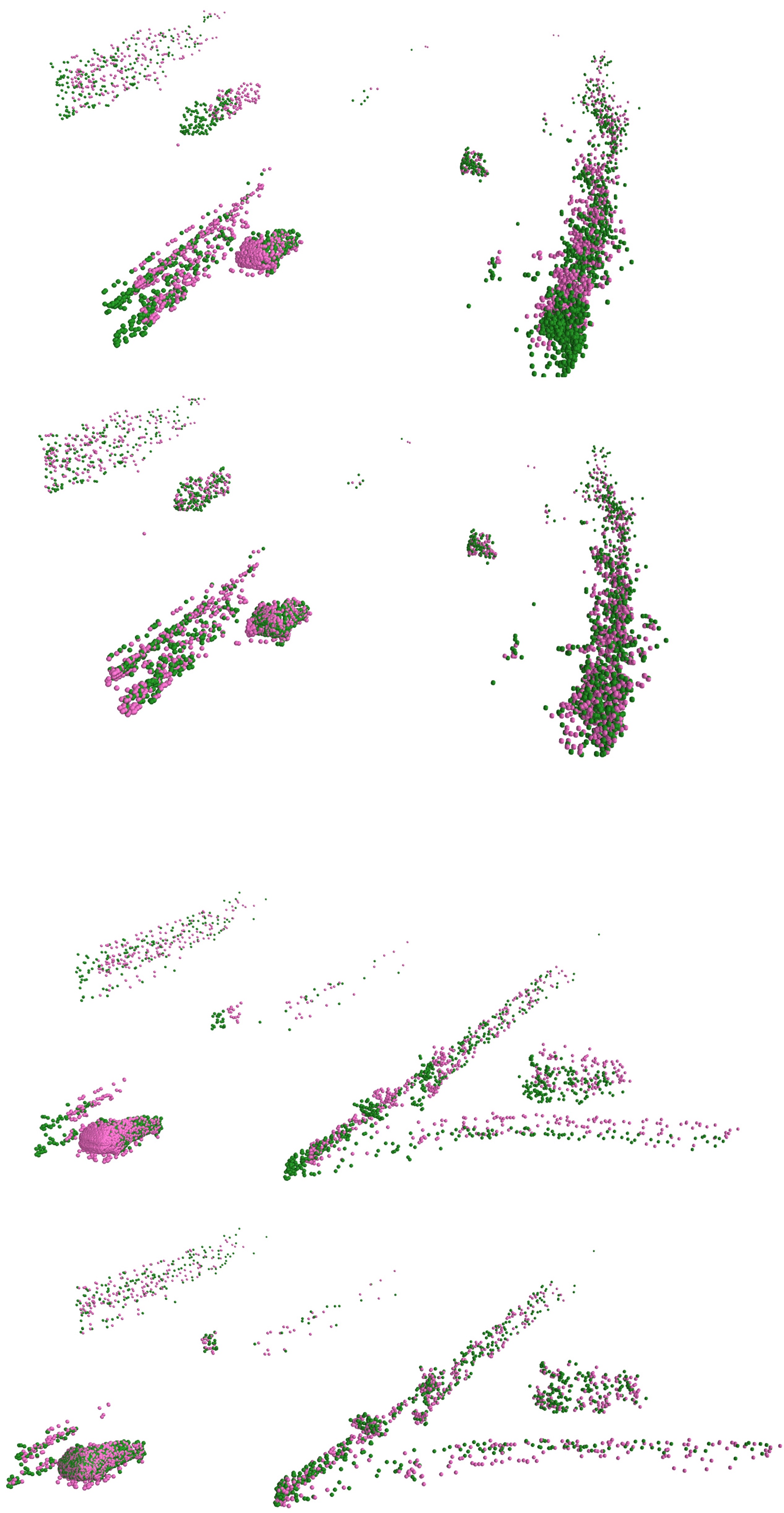
Figure II: Qualitative non-rigid registration results of NDP on KITTI scene flow benchmark. Upper rows are the initial point cloud alignment and low rows are the registered point cloud.

IV. Outlier rejection using Transformer

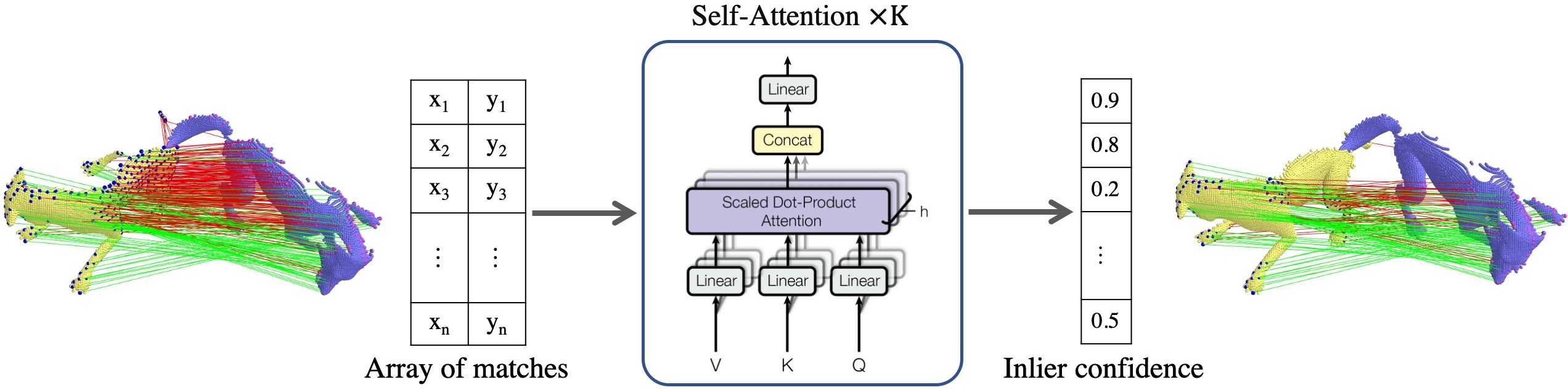
Figure III: Outlier rejection network using Transformer. The red/green lines indicate inliers/outliers.

It is necessary to reject poor correspondences for robust non-rigid registration. Existing learning-based approaches, such as DGR [8] and PointDSC [2], formulate outlier rejection as a binary classification problem, i.e. they use a network to predict the outlier probability of each corresponding point pair. Inspired by these works, we use Transformer to reject outliers. As discussed in DGR [8], inlier correspondences between two rigid scans should form a manifold geometry in 6D space. Similarly, inlier correspondences in non-rigid scenes should also form a submanifold in 6D, because natural deformations are usually locally rigid. Therefore, the motivation is to learn the geometry of inliers in 6D space using transformers.

Fig. III shows the overview of our outlier rejection method. It takes as input an array of 6D coordinates, denoting the corresponding point pairs, and predicts the inlier probability of each correspondence.

We obtain the input correspondence using Lepard [23]. The network consists of a sequence of multi-head self-attention (SA) layers [42], with the head number set to 8. To leverage the spatial consistency of the correspondence, we modify the self-attention layer using the spatial-consistency-guided attention as proposed in PointDSC [2]. The output of the last SA layer is activated through the Sigmoid function that maps the output to range $[0,1]$ as the per-correspondence confidence score. We use weighted binary cross-entropy (BCE) as the loss function for training. The network is trained, validated, and tested on the 4DMatch [23] split. When testing, we treat correspondence with a confidence score below the threshold $\theta=0.3$ as outliers. Fig. IV shows the influence of the threshold $\theta$ for non-rigid registration.

Number of SA layer.

Tab. VII shows the ablation study of number of self-attention (SA) layer. Precision grows with the number of the SA layer. The recall rate becomes stable after using 3 or more layers. By default, our method uses 9 SA layers.

Table VII: Outlier rejection resutls on 4DLoMatch. Following [23], inlier threshold is set to 4cm.

		Number of SA layer
	Input from Lepard[23]	1	2	3	4	5	6	7	8
Precision	55.7 (inlier rate)	63.2	64.7	64.3	74.6	74.3	74.9	76.3	77.1
Recall		58.9	77.0	86.0	80.2	80.2	83.4	80.3	80.1

Outlier rejection confidence.

The precision and recall rate in Tab. VII can not reflect the end-to-end performance for non-rigid registration. We want to find a proper outlier rejection threshold for non-rigid registration. Fig. IV shows the ablation study of the confidence threshold for non-rigid registration accuracy. The optimal confidence threshold lies around 20%-30%. A threshold higher than 60% leads to worse results than not rejecting outliers.

Outlier rejection for registration. Rejecting correspondence outliers gains $+6.83\%$ AccS on 4DMatch/4DLoMatch. See the supplementary for details of outlier rejection.

Table VIII: Ablation study of outlier rejection using LNDP . The confidence threshold is set to 0.3. (In this experiment, we use $L_{2}$ norm for correspondence term).

	4DMatch
Method	EPE$\downarrow$	AccS $\uparrow$	AccR $\uparrow$	Outlier$\downarrow$	Time $\downarrow$
LNDP (w/o outlier rejection )	0.091	54.89	68.39	20.96	2.24
LNDP (Default)	0.078	61.27	74.10	17.50	2.39

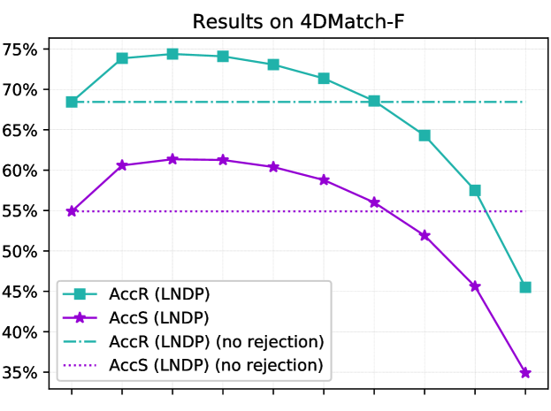
Figure IV: Ablation study of outlier rejection threshold for non-rigid registration.

V. 4DMatch benchmark filtering.

We observe that the original 4DMatch/4DLoMatch benchmarks contain a certain amount of entries that are dominated by rigid motion, i.e. the best rigid fitting already registers most of the points. For fair benchmarking of non-rigid registration, we probabilistically remove point cloud pairs that have near-rigid movements. In the end, we removed around 50% of the entries. Fig. V shows the histogram of the benchmark before and after filtering.

Figure V: Histogram of point cloud registration Accuracy (at 5cm) via the oracle rigid fitting. The left shows the pre-filtered 4DMatch & 4DLoMatch benchmarks, the right shows the filtered benchmarks.

References

- [1] K Somani Arun, Thomas S Huang, and Steven D Blostein. Least-squares fitting of two 3-d point sets. IEEE Transactions on pattern analysis and machine intelligence, pages 698–700, 1987.
- [2] Xuyang Bai, Zixin Luo, Lei Zhou, Hongkai Chen, Lei Li, Zeyu Hu, Hongbo Fu, and Chiew-Lan Tai. Pointdsc: Robust point cloud registration using deep spatial consistency. In Proceedings of the IEEE/CVF Conference on Computer Vision and Pattern Recognition, pages 15859–15869, 2021.
- [3] Paul J Besl and Neil D McKay. Method for registration of 3-d shapes. In Sensor fusion IV: control paradigms and data structures, volume 1611, pages 586–606. International Society for Optics and Photonics, 1992.
- [4] Jean-Yves Bouguet et al. Pyramidal implementation of the affine lucas kanade feature tracker description of the algorithm. Advances in Neural Information Processing Systems, 2001.
- [5] Aljaž Božič, Pablo Palafox, Michael Zollhöfer, Angela Dai, Justus Thies, and Matthias Nießner. Neural non-rigid tracking. arXiv preprint arXiv:2006.13240, 2020.
- [6] Aljaž Božič, Michael Zollhöfer, Christian Theobalt, and Matthias Nießner. Deepdeform: Learning non-rigid rgb-d reconstruction with semi-supervised data. In Proceedings of the IEEE Conference on Computer Vision and Pattern Recognition (CVPR), pages 7002–7012, 2020.
- [7] Che-Han Chang, Chun-Nan Chou, and Edward Y Chang. Clkn: Cascaded lucas-kanade networks for image alignment. In Proceedings of the IEEE Conference on Computer Vision and Pattern Recognition (CVPR), pages 2213–2221, 2017.
- [8] Christopher Choy, Wei Dong, and Vladlen Koltun. Deep global registration. In Proceedings of the IEEE/CVF conference on computer vision and pattern recognition, pages 2514–2523, 2020.
- [9] Nicolas Donati, Abhishek Sharma, and Maks Ovsjanikov. Deep geometric functional maps: Robust feature learning for shape correspondence. In Proceedings of the IEEE/CVF Conference on Computer Vision and Pattern Recognition, pages 8592–8601, 2020.
- [10] Nicolas Donati, Abhishek Sharma, and Maks Ovsjanikov. Deep geometric maps: Robust feature learning for shape correspondence. CVPR, 2020.
- [11] Alexey Dosovitskiy, Philipp Fischer, Eddy Ilg, Philip Hausser, Caner Hazirbas, Vladimir Golkov, Patrick Van Der Smagt, Daniel Cremers, and Thomas Brox. Flownet: Learning optical flow with convolutional networks. In Proceedings of the IEEE International Conference on Computer Vision (ICCV), pages 2758–2766, 2015.
- [12] Jakob Engel, Thomas Schöps, and Daniel Cremers. Lsd-slam: Large-scale direct monocular slam. In Proceedings of the European Conference on Computer Vision (ECCV), pages 834–849, 2014.
- [13] Jean Feydy, Joan Glaunès, Benjamin Charlier, and Michael Bronstein. Fast geometric learning with symbolic matrices. Advances in Neural Information Processing Systems, 33, 2020.
- [14] Jean Feydy, Thibault Séjourné, François-Xavier Vialard, Shun-ichi Amari, Alain Trouve, and Gabriel Peyré. Interpolating between optimal transport and mmd using sinkhorn divergences. In The 22nd International Conference on Artificial Intelligence and Statistics, pages 2681–2690, 2019.
- [15] Andreas Geiger, Philip Lenz, and Raquel Urtasun. Are we ready for autonomous driving? the kitti vision benchmark suite. In Proceedings of the IEEE Conference on Computer Vision and Pattern Recognition (CVPR), pages 3354–3361, 2012.
- [16] Marc Habermann, Weipeng Xu, Michael Zollhoefer, Gerard Pons-Moll, and Christian Theobalt. A deeper look into deepcap. In IEEE Transactions on Pattern Analysis and Machine Intelligence (TPAMI), pages 1–1. IEEE, 2021.
- [17] Amir Hertz, Or Perel, Raja Giryes, Olga Sorkine-Hornung, and Daniel Cohen-Or. Sape: Spatially-adaptive progressive encoding for neural optimization. Advances in Neural Information Processing Systems, 34, 2021.
- [18] Osamu Hirose. A bayesian formulation of coherent point drift. IEEE transactions on pattern analysis and machine intelligence, 43(7):2269–2286, 2020.
- [19] Jiahui Huang, Tolga Birdal, Zan Gojcic, Leonidas J Guibas, and Shi-Min Hu. Multiway non-rigid point cloud registration via learned functional map synchronization. arXiv preprint arXiv:2111.12878, 2021.
- [20] Hao Li, Robert W Sumner, and Mark Pauly. Global correspondence optimization for non-rigid registration of depth scans. In Computer graphics forum, volume 27, pages 1421–1430. Wiley Online Library, 2008.
- [21] Xueqian Li, Jhony Kaesemodel Pontes, and Simon Lucey. Neural scene flow prior. Advances in Neural Information Processing Systems, 34, 2021.
- [22] Yang Li, Aljaz Bozic, Tianwei Zhang, Yanli Ji, Tatsuya Harada, and Matthias Nießner. Learning to optimize non-rigid tracking. In Proceedings of the IEEE Conference on Computer Vision and Pattern Recognition (CVPR), pages 4910–4918, 2020.
- [23] Yang Li and Tatsuya Harada. Lepard: Learning partial point cloud matching in rigid and deformable scenes. IEEE/CVF Conference on Computer Vision and Pattern Recognition (CVPR), 2022.
- [24] Yang Li, Hikari Takehara, Takafumi Taketomi, Bo Zheng, and Matthias Nießner. 4dcomplete: Non-rigid motion estimation beyond the observable surface. arXiv preprint arXiv:2105.01905, 2021.
- [25] Zhengqi Li, Simon Niklaus, Noah Snavely, and Oliver Wang. Neural scene flow fields for space-time view synthesis of dynamic scenes. In Proceedings of the IEEE/CVF Conference on Computer Vision and Pattern Recognition, pages 6498–6508, 2021.
- [26] Miao Liao, Qing Zhang, Huamin Wang, Ruigang Yang, and Minglun Gong. Modeling deformable objects from a single depth camera. In 2009 IEEE 12th International Conference on Computer Vision, pages 167–174. IEEE, 2009.
- [27] Tanwi Mallick, Partha Pratim Das, and Arun Kumar Majumdar. Characterizations of noise in kinect depth images: A review. IEEE Sensors journal, 14(6):1731–1740, 2014.
- [28] Simone Melzi, Jing Ren, Emanuele Rodola, Abhishek Sharma, Peter Wonka, and Maks Ovsjanikov. Zoomout: Spectral upsampling for efficient shape correspondence. arXiv preprint arXiv:1904.07865, 2019.
- [29] Lars Mescheder, Michael Oechsle, Michael Niemeyer, Sebastian Nowozin, and Andreas Geiger. Occupancy networks: Learning 3d reconstruction in function space. In Proceedings of the IEEE Conference on Computer Vision and Pattern Recognition (CVPR), pages 4460–4470, 2019.
- [30] Ben Mildenhall, Pratul P. Srinivasan, Matthew Tancik, Jonathan T. Barron, Ravi Ramamoorthi, and Ren Ng. Nerf: Representing scenes as neural radiance fields for view synthesis. In ECCV, 2020.
- [31] Thomas Müller. Tiny CUDA neural network framework, 2021. https://github.com/nvlabs/tiny-cuda-nn.
- [32] Andriy Myronenko and Xubo Song. Point set registration: Coherent point drift. IEEE transactions on pattern analysis and machine intelligence, 32(12):2262–2275, 2010.
- [33] Richard A Newcombe, Dieter Fox, and Steven M Seitz. Dynamicfusion: Reconstruction and tracking of non-rigid scenes in real-time. In Proceedings of the IEEE Conference on Computer Vision and Pattern Recognition (CVPR), pages 343–352, 2015.
- [34] Maks Ovsjanikov, Mirela Ben-Chen, Justin Solomon, Adrian Butscher, and Leonidas Guibas. Functional maps: a flexible representation of maps between shapes. ACM Transactions on Graphics (TOG), 31(4):1–11, 2012.
- [35] Keunhong Park, Utkarsh Sinha, Jonathan T Barron, Sofien Bouaziz, Dan B Goldman, Steven M Seitz, and Ricardo Martin-Brualla. Nerfies: Deformable neural radiance fields. In Proceedings of the IEEE/CVF International Conference on Computer Vision, pages 5865–5874, 2021.
- [36] Gilles Puy, Alexandre Boulch, and Renaud Marlet. Flot: Scene flow on point clouds guided by optimal transport. In Computer Vision–ECCV 2020: 16th European Conference, Glasgow, UK, August 23–28, 2020, Proceedings, Part XXVIII 16, pages 527–544. Springer, 2020.
- [37] Vincent Sitzmann, Julien Martel, Alexander Bergman, David Lindell, and Gordon Wetzstein. Implicit neural representations with periodic activation functions. Advances in Neural Information Processing Systems, 33:7462–7473, 2020.
- [38] Olga Sorkine and Marc Alexa. As-rigid-as-possible surface modeling. In Symposium on Geometry Processing, volume 4, pages 109–116, 2007.
- [39] Robert W Sumner, Johannes Schmid, and Mark Pauly. Embedded deformation for shape manipulation. ACM Transactions on Graphics (TOG), 26(3):80, 2007.
- [40] Deqing Sun, Xiaodong Yang, Ming-Yu Liu, and Jan Kautz. Pwc-net: Cnns for optical flow using pyramid, warping, and cost volume. In Proceedings of the IEEE Conference on Computer Vision and Pattern Recognition (CVPR), pages 8934–8943, 2018.
- [41] Matthew Tancik, Pratul Srinivasan, Ben Mildenhall, Sara Fridovich-Keil, Nithin Raghavan, Utkarsh Singhal, Ravi Ramamoorthi, Jonathan Barron, and Ren Ng. Fourier features let networks learn high frequency functions in low dimensional domains. Advances in Neural Information Processing Systems, 33:7537–7547, 2020.
- [42] Ashish Vaswani, Noam Shazeer, Niki Parmar, Jakob Uszkoreit, Llion Jones, Aidan N Gomez, Łukasz Kaiser, and Illia Polosukhin. Attention is all you need. In Advances in neural information processing systems, pages 5998–6008, 2017.
- [43] Wenxuan Wu, Zhiyuan Wang, Zhuwen Li, Wei Liu, and Li Fuxin. Pointpwc-net: A coarse-to-fine network for supervised and self-supervised scene flow estimation on 3d point clouds. arXiv preprint arXiv:1911.12408, 2019.
- [44] Qian-Yi Zhou, Jaesik Park, and Vladlen Koltun. Open3D: A modern library for 3D data processing. arXiv:1801.09847, 2018.
- [45] Yi Zhou, Connelly Barnes, Jingwan Lu, Jimei Yang, and Hao Li. On the continuity of rotation representations in neural networks. In Proceedings of the IEEE/CVF Conference on Computer Vision and Pattern Recognition, pages 5745–5753, 2019.