Machine learning the deuteron: new architectures and uncertainty quantification

Abstract

We solve the ground state of the deuteron using a variational neural network ansatz for the wave function in momentum space. This ansatz provides a flexible representation of both the $S$ and the $D$ states, with relative errors in the energy which are within fractions of a percent of a full diagonalisation benchmark. We extend the previous work on this area in two directions. First, we study new architectures by adding more layers to the network and by exploring different connections between the states. Second, we provide a better estimate of the numerical uncertainty by taking into account the final oscillations at the end of the minimisation process. Overall, we find that the best performing architecture is the simple one-layer, state-independent network. Two-layer networks show indications of overfitting, in regions that are not probed by the fixed momentum basis where calculations are performed. In all cases, the error associated to the model oscillations around the real minimum is larger than the stochastic initialisation uncertainties. The conclusions that we draw can be generalised to other quantum mechanics settings.

1 Introduction

Artificial Neural Networks (ANNs) have become routine computational tools in a wide range of scientific domains [1, 2]. Nuclear physics is no exception, and the number of machine learning (ML) tools is increasing steadily [3, 4, 5, 6, 7, 8, 9]. An interesting and relatively recent use of ANNs is the solution of quantum mechanical problems, including in the many-body domain [10, 11]. These methods use ANNs as an ansatz for the many-body wave function, and employ ready-made ML tools to minimise the energy of the system [12, 13]. The first attempts in condensed matter [14, 15] were quickly followed by advances both within [16] and outside the field [5], including quantum chemistry  [17, 18]. A good example in this direction is FermiNet [19], which uses an inherently antisymmetric wave function as an ansatz in a variational approach to solve the many-electron problem.

The methodology that we use to solve the deuteron here is based on the same variational philosophy and stems from Ref. [20]. In that case, we used a minimal, one-layer variational ANN ansatz to describe the wave function of the deuteron (the only $2-$body nuclear bound state) in momentum space. This yields excellent results in comparison with benchmark solutions for the energies and the wave functions, quantified through fidelity measures. Moreover, we estimated the out-of-sample uncertainty of the model by using several random initialisations in the minimisation problem.

The assessment of uncertainties in variational ANN (vANN) is particularly relevant to pinpoint the fundamental limitations of this methodology. There are several systematic errors that are important for many-body vANNs. For instance, network architectures play a key role in determining the convergence properties of the network. Similarly, for a fixed architecture, vANN widths and depths change the expressivity of the network, and are thus fundamental ingredients in providing faithful representations of continuous wave functions. One should explore this systematic uncertainties extensively before reaching conclusions about any intrinsic shortcomings of the vANN method itself.

The deuteron is an excellent test bed for such studies. It is a relatively simple, one-body-like problem, which already includes the complexity of the strong force. Moreover, dealing with a wave function with two different angular momentum states adds an additional level of sophistication. In this manuscript, we extend the elementary approach of Ref. [20] in two different directions. First, we look at somewhat more complex ANN architectures to describe the wave function. This yields insight on the importance of the network architecture and should ultimately provide information on the limitations of the method beyond a specific architecture. Second, we introduce a novel way to compute the out-of-sample error. In particular, we look at oscillations in the energy, which is our cost function, around the real minimum. These oscillations are an additional source of uncertainty, associated to the minimisation process. The analysis of such errors provides a new insight into uncertainty quantification for variational ANN solvers.

This paper is structured in the following manner. In Section 2 we briefly go over the methods used to approach the deuteron problem with ANNs. Section 3 is devoted to the analysis of the numerical results, including their uncertainties. Finally, in Section 4, we draw a series of conclusions and comment on ways in which our work could be expanded and improved.

2 Methodology

The approach that we use to solve the problem is variational. The ANN plays the role of a wave function ansatz, which we denote $\ket{\psi_{\mathrm{ANN}}^{\mathcal{W}}}$. $\mathcal{W}=\{\mathbf{W^{(1)}}$,$\mathbf{W^{(2)}}$,$\mathbf{W^{(3)}}$,$\mathbf{b}\}$ is a set formed by network weights, $\mathbf{W^{(i)}}$, and biases $\mathbf{b}$. In a variational setting, the total energy of the system is the loss function which reads

$$E^{\mathcal{W}}=\frac{\braket{\psi_{\mathrm{ANN}}^{\mathcal{W}}}{\hat{H}}{\psi_{\mathrm{ANN}}^{\mathcal{W}}}}{\braket{\psi_{\mathrm{ANN}}^{\mathcal{W}}}{\psi_{\mathrm{ANN}}^{\mathcal{W}}}}.$$ (1)

The deuteron is the simplest nuclear two-body problem. We solve its structure in momentum space, where we can trivially separate the center of mass from the relative coordinates [21]. Consequently, the wave function of the system depends only on the relative momentum coordinate, $\vec{q}$. Working in momentum space allows us to skip numerically costly derivatives on the wave functions when computing the kinetic energy.

We can further reduce the dimensionality of the deuteron problem via a partial wave expansion, thus separating the dependence on the absolute value of the momentum $q$ from its dependence on angles. For the deuteron, the tensor component of the strong interaction admixes the $S$ ($L=0$) and the $D$ ($L=2$) components of the ground-state wave function. The network will consequently have two different outputs, one for each state. The potential energy term used to compute Eq. (1) mixes these two states in a non-trivial way, so they are not completely independent from each other in the variational setting.

To implement the problem computationally, we use a one-dimensional grid in $q$ with $N_{q}=64$ points. This grid is used to compute the energy integrals in Eq. (1) via quadrature. The loss function is obtained from a global integral, the energy, and is always computed with the same set of momentum grid points. As we shall see later, this can create some issues in deep models. To efficiently capture the low-momentum structure and the high-momentum tails of the wave function, we use a mesh that densely covers the region of low momenta but is sparse in regions of high momenta. We first distribute $N$ Gauss-Legendre points $x_{i}$ between $0$ and $1$, and then extend them tangentially using the transform $q_{i}=\dfrac{q_{\mathrm{max}}}{\tan\dfrac{\pi}{2}x_{N}}\tan\dfrac{\pi}{2}x_{i}\,,$ with $i=1,\cdots,N_{q}$ and $q_{\mathrm{max}}=500$ fm^-1. In this set-up, the overlap $\braket{\psi_{\text{targ}}^{L}}{\psi_{\text{ANN}}^{L}}$ , as well as all analogous integrated quantities, are discretised as follows:

$$\braket{\psi_{\text{targ}}^{L}}{\psi_{\text{ANN}}^{L}}=4\pi\int_{0}^{\infty}\!\!\!dq\,q^{2}\,\psi_{\text{targ}}^{L*}(q)\psi_{\text{ANN}}^{L}(q)\approx 4\pi\sum_{i=1}^{N_{q}}w_{i}q_{i}^{2}\psi_{\text{targ}}^{L*}(q_{i})\psi_{\text{ANN}}^{L}(q_{i})\,,$$ (2)

where $w_{i}$ are the integration weights associated to the tangentially-transformed Gauss-Legendre mesh. Note that because the angular dependence has been removed via a partial wave expansion, all the integrals involve a radial $q^{2}$ term. Note also that all the wave functions are real-valued.

In the following, we present results corresponding to different ANN architectures for the two wave functions, $\psi_{\text{ANN}}^{L}(q)$, with $L=0$ and $2$. Following Ref. [20], we take three identical steps to train all the networks. These three steps are common to most variational Artificial Neural Network (vANN) problems in quantum mechanics [15]. First, we initialise network parameters to uniform random values in the ranges $\mathbf{W^{(1)}}\in[-1,0)$, $\mathbf{W^{(2)}}\in[0,1)$ and $\mathbf{b}\in[-1,1)$. We choose a sigmoid activation function, $\sigma(x)$, which provided marginally better results than the softplus function in Ref. [20].

Second, we train the ANN to mimic a target function that bears a certain degree of physical meaning. We choose a functional form $\psi^{L}_{\mathrm{targ}}(q)=q^{L}e^{-\frac{\xi^{2}q^{2}}{2}}$, which has the correct low-momentum asymptotic values and a reasonable real-space width, $\xi=1.5\,\mathrm{fm}$. In this pre-training step, we use the overlap

$$K^{L}=\dfrac{\braket{\psi_{\text{targ}}^{L}}{\psi_{\text{ANN}}^{L}}^{2}}{\braket{\psi_{\text{targ}}^{L}}{\psi_{\text{targ}}^{L}}\braket{\psi_{\text{ANN}}^{L}}{\psi_{\text{ANN}}^{L}}}$$ (3)

to compute a total cost function, $C$, defined as

$${}C=(K^{S}-1)^{2}+(K^{D}-1)^{2}\,.$$ (4)

Equation (4) is zero if, and only if, the two overlaps $K^{S}=K^{D}=1$. We choose the optimiser RMSProp [1], which dynamically adapts a global learning locally for all the network parameters. Training a medium-sized ANN with $N_{\mathrm{hid}}\approx 20$ hidden nodes usually takes about $10^{4}$ iterations. We point out that this pretraining step is not strictly necessary to achieve a correct energy minimisation, but it helps in guaranteeing a successful energy minimisation with fewer epochs.

In the third and final step, we define a new cost function: the energy, as given in Eq. (1), and we computed it with the momentum quadrature described above. The network is then trained to minimise $E^{\mathcal{W}}$ for $2.5\times 10^{5}$ epochs. We note that the kinetic energy has diagonal contributions in the $L=0$ and $2$ states, but the potential term mixes both states. We choose the N3LO Entem-Machleidt nucleon-nucleon force [22] which is easily implemented in our code as a momentum-dependent potential. We use the PyTorch library [23, 24], which is particularly useful due to its automatic differentiation capabilities [25]. A full version of the code is available on GitHub [26].

2.1 Architectures

The vANN procedure is relatively general, and can be applied to any feed-forward ANN. In the initial exploration of deuteron wave functions of Ref. [20], a minimal approach was chosen deliberately to explore the potential and the limitations of the method in the simplest possible model. We used a single-layer ANN with an increasing number of hidden nodes in order to assess systematics for a fixed architecture. Here, we take a step further and assess the impact of increasing the depth of the ANN which leads to different architectures.

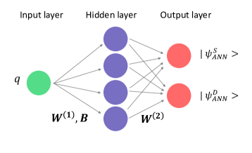
(a) State-connected network with a single hidden layer. For this network, the number of parameters is $N=4N_{\mathrm{hid}}$, with $N_{\mathrm{hid}}$ denoting the number of hidden nodes. Note that the first layer includes a bias.

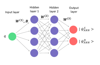
(b) State-connected network with two hidden layers, with $N=\frac{1}{8}N_{\text{hid}}(N_{\text{hid}}+12)$ parameters.

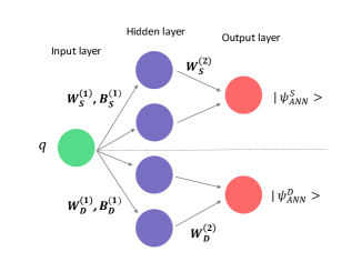
(c) State-disconnected network with a single hidden layer, with $N=3N_{\mathrm{hid}}$ parameters.

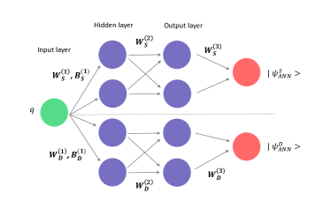
(d) State-disconnected network with two hidden layers, with $N=\frac{1}{4}N_{\mathrm{hid}}\left(N_{\mathrm{hid}}+8\right)$ parameters.

Figure 1: Neural network architectures used in this work.

To this end, we introduce four different ANN architectures, which we show in the four panels of Fig. 1. All our networks have a single input, $q$, and two outputs, $\ket{\Psi^{S}_{\text{ANN}}}$ and $\ket{\Psi^{D}_{\text{ANN}}}$. We distinguish between different configurations depending on how they connect to the two final states. On the one hand, in fully-connected networks, which we dub “state-connected” (sc) networks, all the parameters contribute to both outputs (see the top panels, Figs. 1(a) and 1(b)). On the other hand, “state-disconnected” (sd) networks (bottom panels, Figs. 1(c) and 1(d)) provide independent parameters for each state. One may naively expect sd networks to provide more flexibility (and hence better variational properties) for the two wave functions.

In addition to the state dependence of the network, we also explore architecture systematics in terms of depth. We implement both sc and sd networks with one (left panels) and two (right panels) layers. In the following, we use the acronyms $n$sc and $n$sd ($n=1,2$), with $n$ the number of layers, to refer to the 4 architectures explored in this work. We stress that in Ref. [20] we only looked at the $1$sc architecture. The motivation to explore other architectures and, in particular further depths, is the widely held belief that deep ANNs outperform their shallow single-layered counterparts [27].

In the initial layer of all four architectures, we introduce both weights $\mathbf{W^{(1)}}$ and biases $\mathbf{b}$. In contrast, all the second (and/or third) layers only have weights, $\mathbf{W^{(2)}}$ ($\mathbf{W^{(3)}}$). For clarity and completeness, we provide the functional form of the four networks. For the one-layer $1$sd configurations, the wave function ansatz reads as

$${}\psi^{L}_{\mathrm{ANN}}(q)=\sum^{N_{\mathrm{hid}}/2}_{i=1}W^{(2)}_{i,L}\sigma\left(W^{(1)}_{i,L}q+B_{i,L}\right).$$ (5)

The corresponding $1$sc contribution is obtained by setting $N_{\mathrm{hid}}/2\rightarrow N_{\mathrm{hid}}$ and using $L-$independent $\mathbf{W^{(1)}}$ and $\mathbf{B}$ parameters. When $2$ layers are included, in contrast, the sd ansatz is more complex, and becomes the sum of sums of two nested activation functions,

$${}\psi_{\mathrm{ANN}}^{L}(q)=\sum_{i=N_{\mathrm{hid}}/2+1}^{N_{\mathrm{hid}}}W^{(3)}_{i,L}\sigma\left(\sum_{j=1}^{N_{\mathrm{hid}}/2}W^{(2)}_{j,L}\sigma\left(W_{j,L}^{(1)}q+B_{j,L}\right)\right).$$ (6)

One can again easily manipulate the previous expression to obtain a $2$sd wave function.

The relation between the total number of hidden neurons, $N_{\mathrm{hid}}$, and the total number of variational parameters, $N$, is different for each architecture. The relations $N(N_{\mathrm{hid}})$ are shown in the captions of Fig. 1 for each network configuration. One-layer networks have a linear $N(N_{\mathrm{hid}})$ relation, whereas the relation for two-layer networks is quadratic. In other words, for the same $N_{\text{hid}}$, two-layer networks will usually involve a much larger number of parameters than one-layer models, and one may expect overfitting to become an issue. Whereas for the $1$sc architecture the number of hidden nodes is unrestricted so long as $N_{\text{hid}}>2$, the $2$sc architecture must have $N_{\text{hid}}>4$ with $N_{\text{hid}}$ even. Likewise, the $1$sd network must have an even $N_{\text{hid}}$. In contrast, for the $2$sd network, $N_{\text{hid}}$ must increase $4$ units at a time.

2.2 Learning process

The results we present are obtained with the four network configurations and a sigmoid activation function. We minimise the energy cost function using RMSProp with hyperparameters $\epsilon=10^{-8}$ and a momentum $\beta=0.9$. We set the learning rate to $10^{-2}$ and explore the $N_{\mathrm{hid}}$ dependence using the values $N_{\mathrm{hid}}\in\{20,30,40,60,80,100\}$ (in the 2sc architecture we change $N_{\mathrm{hid}}=30\rightarrow N_{\mathrm{hid}}=32$). To explore the full flexibility of the wave function ansätze, we optimise the networks by minimising the overlap loss function for $2\times 10^{3}$ epochs of pre-training, followed by $2.5\times 10^{5}$ epochs of energy minimisation. Rather than doing this a single time, we use $20$ different random initialisations and display mean values and standard deviations obtained with all these runs. With this, we explore the out-of-sample bias of the network and we attempt to draw generic conclusions for the architecture network, rather than for a single, specific network model.

We typically perform more than $20$ initialisation runs, with the exact number depending on the architecture and $N_{\text{hid}}$. Not all of these runs converge or, if they do, they may not have converged to meaningful values, close enough to the minimum. Figure 2 shows the rate of convergence of different architectures as a function of $N_{\text{hid}}$. This is obtained as the ratio of the number of converged models, $N_{\text{con}}$, to the total set of model initialisations, $N_{\text{tot}}$, $r=N_{\text{con}}/N_{\text{tot}}$. As a selection criterion to compute $N_{\text{con}}$, we define converged models as those that provide a final energy within the range $E\in(-2.220,-2.227)$ MeV. Whenever more than $20$ initialisations lead to converged results, we randomly pick $20$ states to have representative, but also homogeneous, statistics across the $N_{\mathrm{hid}}$ domain. We stress the fact that these rates are obtained from initialisations with a pretraining step. With no pretraining, all models show slower convergence rates. We take this difference as an indication of the fact that pretraining is effective in providing a physical representation of the ANN wave function. Initally non-pretrained networks may occasionally lead to accurate results, but are likely to require many more energy minimisation epochs.

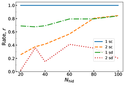
Figure 2: Convergence rate of the four network architectures as a function of the number of hidden neurons. The rate (vertical axis) is defined as the ratio between the number of models that converge and the total number of trained models, $N_{\text{con}}/N_{\text{tot}}$.

Going back to Fig. 2, we find that the one-layer configurations provide better convergence rates than their two-layer counterparts in almost all the range of $N_{\mathrm{hid}}$. The $1$sc network (solid line) has a perfect convergence rate. The $1$sd architecture (dash-dotted line) provides a relatively good convergence rate, with $r>70\%$ relatively independent of the value of $N_{\text{hid}}$. We attribute these similarities to the idea that both pretraining and training are more easily done with a single layer ANN.

In contrast, two-layer networks start with a relatively low convergence rate. In architecture $2$sc we have $r\approx 20\%$ for $N_{\text{hid}}=20$, and the rate increases in a relatively steady and linear fashion up to $r\approx 80-95\%$ for $N_{\text{hid}}=100$. In architecture $2$sd we find even lower convergence rates, $r\approx 2\%$ for $N_{\text{hid}}=20$, and an erratic behaviour in terms of $N_{\text{hid}}$. The stark differences in convergence rates between one and two-layer ANNs may be due to a variety of factors. On the one hand, network parameter initialisation may be an issue. Network parameters in different domains than the ones we prescribe at the moment may provide better starting points. On the other hand, we fix the total number of energy minimisation epochs and the current rate may just be an indication that smaller two-layer networks simply take, with RMSprop, a larger number of epochs to converge. Finally, two-layer networks may be problematic in terms of the sigmoid activation function, which is prone to a vanishing gradients issue [28, 29]. This should be accentuated in deeper (as opposed to shallow one-layer) networks. Along these lines, having few neurons increases the probability that all of them become frozen, which may explain why low $N_{\text{hid}}$ models have a harder time converging. An activation function like softplus or ReLU may work better with $2$-layer architectures. Initial tests with the softplus function do in fact indicate an improvement in convergence rates for $2-$layer networks.

2.3 Error analysis

In addition to different network architectures, we examine two types of uncertainties. First, as we have just explained, we run $20$ minimisations for different $N_{\text{hid}}$ values and network architectures. We take the standard deviation of these $20$ results as a measurement of the uncertainty related to the stochastic minimisation process. This out-of-sample error, which was also explored in Ref. [20], is represented in terms of dark bands in the figures of the following section. It tends to be a relatively small error, of the order of a fraction of a keV in energy.

Second, even after a full minimisation, our results still show some residual oscillations. These oscillations are typically within $1\%$ of the total energy. If we assume that the oscillations happen around the minimum value of $E^{\mathcal{W}}$, we can estimate the true energy minimum by averaging over these oscillations. The oscillation amplitude can then be used to quantify an additional source of uncertainty, associated to the minimiser. To determine this error, we take a trained model and let it evolve for $300$ additional epochs - a process which we call post-evolution. The number of post-evolution epochs is small enough so that the mean value does not change during the process, but also large enough to observe periodicity in the oscillations.

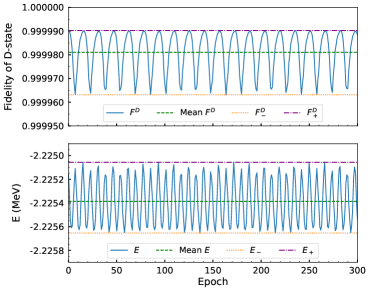
Figure 3: Top panel: D-state fidelity post-evolution of a trained model with architecture $1$sd and $N_{\mathrm{hid}}=40$ hidden neurons. Bottom panel: total energy evolution of the same model as in the top panel.

We illustrate this behaviour in Fig. 3. The top panel shows the evolution of the $D-$state fidelity $F^{D}$ over the $300$ post-evolution epochs for a $1$sd network with $N_{\text{hid}}=40$. Here, we define $F^{L}$ as the overlap between the ANN and benchmark (obtained via exact diagonalisation) wave functions in analogy to Eq. (3). The solid blue line, corresponding to the fidelity at every epoch, displays clear oscillations that are asymmetric with respect to a mean value of $F^{D}\approx 0.99998$. To account for the asymmetry in the oscillating behaviour, we assign an upper and lower error estimate. The upper value corresponds to the maximum value across the post-evolution phase - $\delta F^{D}_{+}=0.00001$ (dash-dotted line), in the case shown in the figure. In contrast, the lower value is significantly lower for this specific example, leading to $\delta F^{D}_{-}=0.00002$ (dotted line). The bottom panel of Fig. 3 shows the energy (solid line) as a function of the post-evolution epoch. The energy oscillates around the mean value (dashed line), and the top and bottom bounds of this oscillations are shown in dash-dotted and dotted lines respectively. In this particular example, the mean value of the energy is $E^{\mathcal{W}}\approx-2.225\,\mathrm{MeV}$, with oscillation errors $\delta E^{\mathcal{W}}_{+}=0.4\,\mathrm{keV}$ and $\delta E^{\mathcal{W}}_{-}=0.4\,\mathrm{keV}$. We note that these values are typical for almost any number of neurons, and are extremely small, less than $0.1\%$ of the total energy value.

In order to take into account the stochastic out-of-sample uncertainty in these oscillations, we repeat the process above $20$ times for each network configuration ($N_{\mathrm{hid}}$). As explained earlier, we extract central values for the different physical quantities by taking the average over the $20$ mean values. We quote post-evolution oscillation errors that also include this stochastic element. In other words, both upper and lower bounds are calculated by averaging over 20 individual post-evolution runs. In a cost function with no near multiple minimums of similar heights, all oscillations should happen around the same minimum, and the mean values of $E^{\mathcal{W}}$ should all be similar. This, in tandem with the fact that we estimate the stochastic $\delta E^{\mathcal{W}}$ as the standard deviation, leads us to expect small stochastic errors and comparatively bigger oscillation errors. We confirm this expectation in the following section.

3 Results

3.1 Energy

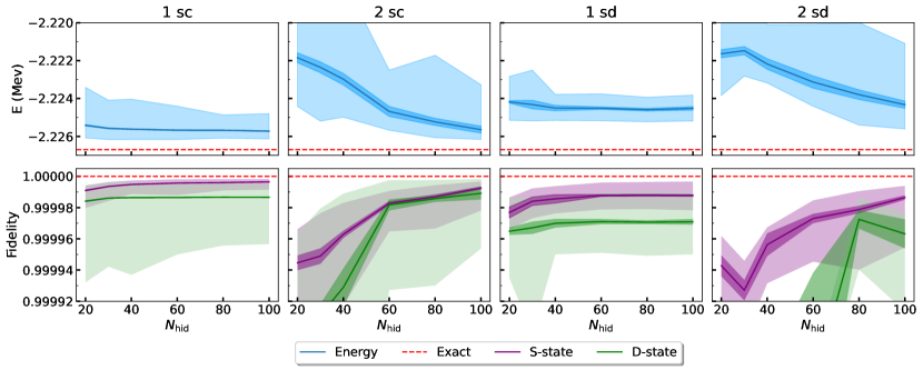
Figure 4: Top panels: energy as a function of the number of hidden nodes. Different panels correspond to the network architectures of Fig. 1. Lines represent central values obtained with $20$ stochastic initialisations. Dark bands show the associated standard deviations (stochastic uncertainty), whereas light bands show the post-evolution oscillation uncertainty. The dashed red lines is the benchmark value. Bottom panels: the same for the fidelity of the ANN wave function with respect to the benchmark for the $S$ (purple) and $D$ (green) states.

The two quantities that we use as indicators of the quality of our final trained models are the energy and the fidelity, represented in the top and bottom panels of Fig. 4, respectively. The four columns correspond to the the different network architectures of Fig. 1. As explained earlier, the solid dark lines in Fig. 4 indicate the central values. We show two different types of uncertainties for each quantity. Firstly, stochastic uncertainties associated to $20$ different initialisations are shown using dark colour bands. Secondly, post-evolution oscillation uncertainties are displayed with pale colours. A key finding of our work is that post-evolution uncertainties are always larger than stochastic uncertainties.

Before discussing uncertainties, we want to stress the quality of the results. As discussed in the context of Fig. 2, the ANNs used to generate these results have been preselected to lie in the range $E\in(-2.220,-2.227)$ MeV. Therefore, all these models already lie within $0.3\%$ of the final energy result. For some architectures, the rate of convergence to this energy window is not $100\%$. Yet, converged results provide energy values which, according to the stochastic uncertainty, are well within $1$ keV (or $0.04\%$) of each other. Post-evolution uncertainties are much larger than stochastic uncertainties, but are typically smaller than $4$ keV (or $0.2\%$). We take this as an indication that all these ANNs provide faithful, high-quality representations of deuteron wave function. While none of the models shown here are able to reach the real minimum even when the post-evolution lower bounds are considered, the distance between the lower bound and the real minimum is always less than $2$ keV. Our analysis indicates that this limitation is due to the fact that the network cannot always distinguish between the $S-$ and $D-$state contributions in high-momentum regions, where the two wave functions are equally small. Ultimately, this limitation only has minor consequences, of a fraction of a percent, in the total energy. As an important conclusion of this analysis, we find that the simplest architecture, $1$sc, provides the more stable and overall best performing results.

An interesting conclusion of Fig. 4 is that state-disconnected architectures perform seemingly worse than state-connected networks. One could have expected the opposite, on the basis that disconnected architectures may provide more independent flexibility for the $\psi^{S}$ and $\psi^{D}$ wave functions. One possible explanation for this behaviour is as follows. Within a single minimisation epoch, the optimiser proposes steps based on the backpropagation of gradients. Changes in parameters associated to the $S-$state are thus immediately propagated to the $D$ state in a fully connected configuration. In contrast, in the disconnected case, these changes do not necessarily affect the $D$ state. In spite of having less parameters than connected architectures, the training may take longer due to this effect.

We now proceed to discuss the $N_{\text{hid}}$ dependence of the results. We find two very different trends depending on the depth of the network. One-layer network results are relatively independent on the network width. In other words, in terms of energy (but also in terms of fidelity), models with $N_{\text{hid}}\approx 30$ are as good as models with $N_{\text{hid}}=100$. In contrast, the two-layer models display a clear improvement in energy for small values of $N_{\mathrm{hid}}$. This suggests that two-layer networks with small values of $N_{\mathrm{hid}}$ have not managed to reach the full minimum after $2.5\times 10^{5}$ epochs. Single-layer models have notably less parameters and can thereby be trained faster than their two-layer counterparts. In fact, snapshots of the minimisation process indicate that two-layer models with few neurons are still learning at the end of the $2.5\times 10^{5}$ epochs. The decrease in energy as $N_{\mathrm{hid}}$ increases extends to the whole range of $N_{\mathrm{hid}}$ in architecture $2$sc and $2$sd. The post-evolution uncertainties for these two-layer models are relatively big and almost compatible with a constant value of energy.

In addition to central values, the dependence of uncertainties in $N_{\text{hid}}$ is informative. The stochastic uncertainties are relatively constant across all values, but are marginally larger for two-layer models. Post-evolution errors for one-layer networks are on the order of $\approx 2$ keV, with a mild decreasing dependence on network width. In contrast, two-layer network post-evolution uncertainties are as large as $6$ ($4$) keV for low (high) $N_{\text{hid}}$ values. Following the same argument about the energies of such models, this can be understood by realising that the updates in $\mathcal{W}$ from RMSProp affect both $\psi^{S}$ and $\psi^{D}$ in the state-connected case (as opposed to the state-disconnected case). One expects this may lead to larger energy variations and, hence, bigger oscillations.

The difference in oscillation errors can also be understood in terms of frozen neurons. Two-layer models that converge will not have many frozen neurons, and given that such models have comparatively many more parameters than their one-layer counterparts, the changes in $\mathcal{W}$ are expected to be comparatively bigger. This, when the minimum of the oscillation is not deep enough, can cast the model away from the minimum which is reflected in large, irregular oscillations. The argument above also explains why the stochastic errors are comparatively bigger in two-layer models: big, non-regular oscillations are prone to yield different central values, which directly translates to bigger stochastic errors.

3.2 Fidelity

The bottom panels of Fig. 4 also provide an insight on the model quality after minimisation. Again, we highlight that overall the fidelities are extremely close to benchmark values, within a fraction of a percent in all cases. We find general conclusions in terms of network width that are in line with those we found for the energy. Across all architectures and network depths, the fidelity of the $S-$state is better than that associated to the $D$-state. Not only are the central values of $F^{S}$ closer to one, but post-evolution uncertainties are significantly smaller for this state. This is in contrast to the much smaller stochastic uncertainty, which is of the same size for both states.

When it comes to the $N_{\text{hid}}$ dependence of the results, we find again that one-layer networks are relatively independent of the network width. Overall, networks perform better with $1$sc than with $2$sc architectures as measured by overlaps that are closer to one, although they have relatively similar uncertainties. The fidelities of the $1$sd architecture improve as the width increases. Again, we interpret this result in terms of incomplete learning for networks with fewer parameters. The behaviour of the $2$sd networks (rightmost panels) is more erratic. The $S-$state fidelity is relatively close to the benchmark and seemingly improves with $N_{\text{hid}}$. In contrast, the $D-$state fidelity is closer to one for $N_{\text{hid}}=80$, and subsequently its quality decreases. We take this as a sign that such architectures with $N_{\text{hid}}$ values larger than $80$ may be problematic and, in fact, we show in the following subsection that overfitting is an issue in this region. Finally, we stress again that there is no observable bias-variance trade-off in the fidelities.

3.3 Wave functions

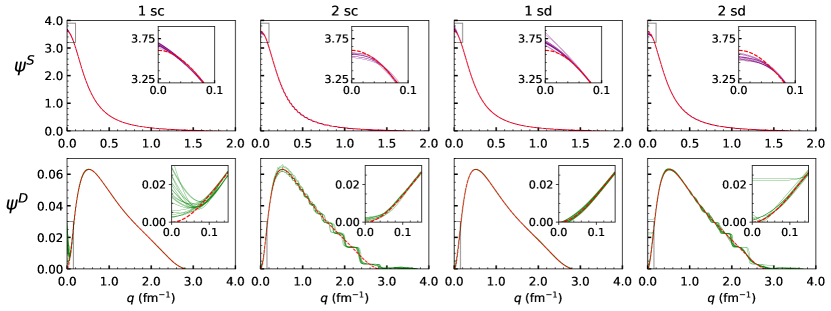
Figure 5: Top panels: $20$ instances of the $S-$state wave function as a function of momentum, for each of the 4 architectures considered here for $N_{\text{hid}}=100$. The dashed line represents the benchmark wave function. The insets focus on the region around the origin, $q\approx 0$. Bottom panels: the same for the $D-$state wave function. Note the difference in scales of the momentum in both rows.

We now turn our attention to analysing directly the ANN outputs: the wave functions. This is an instructive exercise that allows us to have clearer and more local indicators of model quality, in addition to the information provided by integrated quantities such as the energy or the fidelity. We show $20$ different instances of the wave functions of the $S-$ (top panels) and $D-$states (bottom panels) in Fig. 5. To show the “best” possible wave functions, we focus on the number of hidden nodes $N_{\text{hid}}$ that provide the lowest (central value of the) energies. For all four architectures considered, this corresponds to $N_{\text{hid}}=100$. By looking at these instances directly, one gets an idea of the possible spread of variationally evolved models. Overall, we find that all networks provide very similar, high-quality representations of the benchmark wave function which is shown in dashed lines.

In most cases, the largest discrepancies occur towards the origin. As explained in Ref. [20], the presence of a $q^{2}$ factor in the energy integrals allows the networks to push a large amount of variance towards the origin. In other words, changing the wave function near the origin has no reflection on the global cost function. The large variance can be seen in the insets of all panels which show the behaviour of the wave functions close to the origin. For the $S-$state, one-layer models have relatively linear behaviours as $q\to 0$, whereas $2-layer$ networks saturate close to the origin. None of these behaviours matches the benchmark, showed in dashed lines, in this limit. We note that the $20$ realisations provide a relatively similar amount of deviations around a central value. This is in contrast to the $D-$state wave function of the $1$sc architecture, which has a large variation around the origin, in spite of providing the best overall energies.

Unlike in Ref. [20], we display the wave functions of Fig. 5 in a linear and denser grid of points than the one used to compute energy quadratures. This allows us to investigate whether the network is able to learn efficiently not only the properties at the mesh points or the origin, but also the continuity of the wave function across a set of points at finite momentum. Indeed, we observe a step-like behaviour in the two-layer $D-$state wave functions (bottom panels). These steps occur precisely in the vicinity of each quadrature mesh point and they are more easily seen at high momenta where mesh points are relatively spaced apart. Clearly, two-layer networks have enough flexibility to generate horizontal steps around these points. In other words, the networks learn the properties of the wave function only locally around the meshpoints and interpolate in a stepwise fashion between them. We take this as another, different sign of out-of-sample uncertainty. We stress that the step do not occur in simpler, less flexible one-layer models. We speculate that the lack of flexibility of such models forces them to behave in a more continuous fashion. Further, these effects are not detected in integrated quantities, since the quadrature meshpoint values are well reproduced by all the networks. In other words, in our set-up, the regions between mesh points do not contribute to the loss functions. Therefore, the network can push the variance to these regions with virtually no observable effect.

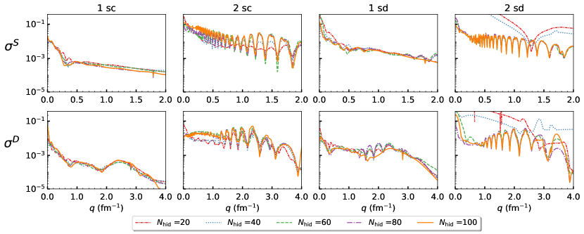
Figure 6: Top panels: standard deviation associated to $20$ instances of the $S-$state wave function as a function of momentum, for each of the 4 architectures considered here. Different line styles correspond to different $N_{\mathrm{hid}}$ values. Bottom panels: the same for the $D-$state wave function. Note the difference in scales of the momentum in both rows.

Figure 6 provides further insight into the structure of the wave function variance in our models. The variance here is estimated as the standard deviation associated to the $20$ model initialisations of our networks. The different line styles in the figure correspond to different values of $N_{\text{hid}}$. Top (bottom) panels show $S$ ($D$) state variances. It is quite clear from these figures that the overall variance at finite momentum is relatively independent of the network width. Moreover, most network models have maximum variances towards the origin which is in line with Fig. 5. $1-$layer networks have relatively flat declines with momentum, and saturate at values of the order of $\sigma\approx 10^{-3}$.

In contrast, $2-$layer networks have pronounced oscillatory values. The oscillation positions have a one-to-one correspondence with the plateaus in Fig. 5. Variance minima occur at the quadrature mesh points, and maxima happen in between. The oscillation minima (eg the smallest uncertainties) have variances which are similar to the $1-$layer case. This is a clear indication that the network has learned locally the wave functions of the system at the quadrature mesh grids, but is overfitting the values in between which are not penalised by the cost function. Note also that the variance for the $2$sd models with low $N_{\text{hid}}$ differs from the general trend. This is due to the poor adaptiveness of such architectures. In fact, some of these converged wave functions bear little resemblance to the exact ones, despite the fact that their energy is still within the range of Fig. 4. We discuss potential mitigation strategies to these problems in the following sections.

Before discussing solutions to this problem, we want to quantify its relevance. To this end, we generate wave function models in a new uniform $10^{3}$-point mesh in the interval $[0,5]$ fm^-1. We use this new linear mesh to compute, in quadrature, the overlaps of the network models to the benchmark wave function as well as the total energy. To summarise our findings, we show in Table 1 the results of this exercise for 2 different models. On the one hand, the $1$sd model with $N_{\mathrm{hid}}=100$ (top row) shows almost no signs of overfitting. In contrast, the middle row shows results for the $2$sd architecture with $N_{\mathrm{hid}}=100$, which has significant overfitting. The bottom row quotes the values obtained with a benchmark wave function, obtained in the very same uniform mesh.

	$F^{S}$	$F^{D}$	$E$ (MeV)
$1$sd	$0.99997\pm 0.00001$	$0.99994\pm 0.00003$	$-2.2172\pm 0.0008$
$2$sd	$0.9992\pm 0.0004$	$0.993^{+0.007}_{-0.012}$	$-2.0\pm 0.3$
Benchmark	1	1	-2.22486

Table 1: Fidelity and energies of the $1$sd and $2$sd architectures in a uniform mesh, where the overfitting is captured. Each value is the mean over the set of $20$ initialisations, and the errors are the associated standard deviations.

First, we discuss the fidelities reported in the first and second columns of Table 1. These are computed in the uniform mesh, as opposed to the results presented in Fig. 4 for the original quadrature. For the $1$sd model, the fidelities are practically the same, close to $1$ up to the fourth or fifth significant digit. This is due to the fact that the model has barely any overfitting. The fidelities of the $2$sd model are, however, one and two orders of magnitude further away from one than those reported in Fig. 4. We take this as an early indication of potential overfitting.

A second, stronger indication comes from the energies in the final column. These values should be compared to the benchmarks in the same uniform mesh, reported in the bottom row. Two conclusions can be drawn here. First, the energy values obtained in this mesh are significantly worse than the exact ones. Whereas for the $1$sd value the energy lies within a fraction of a percent of the benchmark, for the $2$sd model the model is only accurate up to $10\%$ of the total energy. Second, the stochastic uncertainties are significantly larger than those reported in Fig. 4. For the $1$sd network, the values are relatively competitive, of the order of $1$ keV. The $2$sd model has stochastic uncertainties of $300$ keV, several orders of magnitude higher.

This substantial increase in stochastic uncertainty, as well as the important change in energy central values, indicate that overfitting is particularly problematic for $2-$layer networks. Among other things, this indicates that the results shown in Fig. 4 are not fully representative of the true values of $2-$layer networks. The general behaviour of these quantities as a function of $N_{\mathrm{hid}}$ is, however, expected to remain the same.

Having quantified the importance of overfitting, we now discuss its causes. The differences between the exact and predicted wave functions appear almost exclusively in two-layer models. These models have comparatively more parameters, which are presumably redundant. Two-layer networks can “hide” this redundancy in regions with little or no contributions to the cost functions, either towards the origin or in regions in-between fixed quadrature mesh points. We stress that having too many parameters does not restrict the ANN outputs, but it may increase the difficulty of the task assigned to the optimiser. The easy path out in this case is to overfit the data.

Moreover, as one increases the number of parameters, the network may find multiple ways of fitting the data set evaluated on the same fixed $N_{q}$ mesh points. In other words, larger networks can represent the same wave functions in many different ways, and as the number of parameters grow, so do the number of ways in which a network can represent the wave functions. This is usually identified as a bias-variance trade-off.

We now speculate how to mitigate the overfitting effects on the wave functions. An obvious alternative is to try and increase the mesh density. One expects that in regions which are densely covered by the mesh, the networks may not have enough freedom to develop the artificial plateaus observed in Fig. 5. Just as in traditional variational models, improving the quality of the (momentum-space) basis by, say, increasing $N_{q}$, may also be beneficial in terms of the optimisation. Alternatively, one can envisage a set-up in which meshes change from epoch to epoch. If such changes are entirely stochastic, one could rephrase them as traditional variational quantum Monte Carlo implementations, although these are not usually formulated with non-local interactions like the Entem-Machleidt potential. Alternatively, one could work with deterministic meshes but change the total number of meshpoints or the positions at each epoch. In the most favourable scenario, one would expect to find a network that does not memorise specific data mesh points, but rather learns the wave function structure. In the end, any such strategy would try to enforce a network learning process that is independent of the specific quadrature that is used to compute the global cost energy function. In other applications of supervised learning, the quality of the local cost function is quantified via comparison to a validation dataset from which the network doesn’t learn but merely compares.

4 Conclusions and future outlook

In this work, we use vANNs to compute the ground state properties of the deuteron with a realistic hamiltonian. To this end, we discretise the problem in a fixed mesh on the relative momentum coordinate. We use standard ML tools, based on Pytorch, to pre-train our models and subsequently minimise the energy for a fixed number of epochs.

High-quality solutions for the variational wave function were already obtained in Ref. [20] with a similar set-up. We extend this work here in two directions, aimed at identifying fundamental limitations of the vANN approach. First, we look at different ANN architectures, increasing the number of layers and treating the connection to the output states in a connected or disconnected fashion. Second, we identify a new source of uncertainty associated to the oscillations around the final energy minimum. Third, by carefully analysing the wave function outputs, we identify conditions in which finite-momentum overfitting arises.

All vANNs models provide excellent results for the energies and fidelities, when compared to benchmark wave functions. We find that ANNs do not have to be specially tailored to perform well at a problem.

By looking at the rate of model convergence for different architectures, we find a first qualitative sign that two-layer networks have a harder time minimising the energy than their one-layer counterparts. In terms of model uncertainties, the post-evolution oscillation errors dominate over the stochastic initialisation errors, but they remain relatively small (of the order of $6$ to $8$ keV) across a wide range of network widths. When it comes to the structure of the network, state-connected networks, with output nodes that are connected to the internal hidden layer, provide marginally better results than state-disconnected architectures.

Overall, we find that two-layer networks provide worse results than one-layer models. This may have been expected since the input layer is based on a single, positive-defined degree of freedom (the magnitude of the relative momentum, $q$). Central values of the energy are less attractive, and the stochastic and post-evolution uncertainties are larger. We also identify a dependence on the number of hidden nodes which is absent in the one-layer case. Representing the wave functions of these models at grid points that are not used in the minimisation process, we find anomalous horizontal steps between mesh points for the two-layer models. These are clear signs of network overfitting. It seems that, during the minimisation process, the network is able to push some of the redundant dependence of parameters into these regions, which do not contribute to the energy cost function. This is analogous to the observation of a large variance (in terms of wave function values) around the origin, where the spherical $q^{2}$ factor allows the network to change values arbitrarily around $q\approx 0$ without affecting the total energy. Unlike the situation at the origin, however, a change of integration mesh for the energy can easily detect the degradation of the model associated to overfitting at finite momentum. We find that, in the new mesh, the fidelities with respect to benchmark wave functions become worse. The energy values in a different mesh are also substantially less attractive. The associated stochastic uncertainty increases, reaching up to $300$ keV in some cases.

While unveiling the internal behaviour of the ANN is hard, the comparison between different architectures certainly sheds some light on the fundamental limitations of these variational methods. When it comes to presenting wave functions that depend on a single continuous variable, our results indicate that one-layer networks provide a better starting point than the more complex two-layer approaches. This effect may be due to the fixed (if long) total number of epochs, but other observations indicate that overfitting arises much more easily in deeper networks. Similarly, our results suggest that the network can tackle states with different quantum numbers in a fully connected configuration. In training ANNs to represent continuous quantum systems, non-fixed grid methods may provide superior learning capabilities. Overall, this experience provides useful ideas to build more sophisticated nuclear models and tackle more difficult problems, including those of a many-body nature.

References

References

- [1] Mehta P, Bukov M, Wang C et al. 2019 Phys. Rep. 810 1–124 (Preprint arxiv:1803.08823) URL https://doi.org/10.1016/j.physrep.2019.03.001
- [2] Carleo G, Cirac I, Cranmer K, Daudet L, Schuld M, Tishby N, Vogt-Maranto L and Zdeborová L 2019 Rev. Mod. Phys. 91(4) 045002 (Preprint arXiv:1903.10563) URL https://link.aps.org/doi/10.1103/RevModPhys.91.045002
- [3] Boehnlein A, Diefenthaler M, Fanelli C, Hjorth-Jensen M, Horn T, Kuchera M P, Lee D, Nazarewicz W, Orginos K, Ostroumov P, Pang L G, Poon A, Sato N, Schram M, Scheinker A, Smith M S, Wang X N and Ziegler V 2021 Artificial intelligence and machine learning in nuclear physics URL https://arxiv.org/abs/2112.02309
- [4] Utama R, Piekarewicz J and Prosper H B 2016 Phys. Rev. C 93 014311 (Preprint 1508.06263) URL https://link.aps.org/doi/10.1103/PhysRevC.93.014311
- [5] Gao X and Duan L M 2017 Nat. Commun. 8 1 (Preprint arxiv:1701.05039) URL https://doi.org/10.1038/s41467-017-00705-2
- [6] Lasseri R D, Regnier D, Ebran J P and Penon A 2020 Phys. Rev. Lett. 124(16) 162502 (Preprint arXiv:1910.04132) URL https://link.aps.org/doi/10.1103/PhysRevLett.124.162502
- [7] Niu Z M, Liang H Z, Sun B H, Long W H and Niu Y F 2019 Phys. Rev. C 99(6) 064307 URL https://link.aps.org/doi/10.1103/PhysRevC.99.064307
- [8] Wang Z A, Pei J, Liu Y and Qiang Y 2019 Phys. Rev. Lett. 123 122501 (Preprint arxiv:1906.04485) URL https://link.aps.org/doi/10.1103/PhysRevLett.123.122501
- [9] Raghavan K, Balaprakash P, Lovato A, Rocco N and Wild S M 2021 Phys. Rev. C 103(3) 035502 (Preprint arXiv:2010.12703) URL https://link.aps.org/doi/10.1103/PhysRevC.103.035502
- [10] Adams C, Carleo G, Lovato A and Rocco N 2021 Phys. Rev. Lett. 127(2) 022502 (Preprint arxiv:2007.14282) URL https://link.aps.org/doi/10.1103/PhysRevLett.127.022502
- [11] Gnech A, Adams C, Brawand N, Carleo G, Lovato A and Rocco N 2021 Few-Body Syst. 63 7 URL https://doi.org/10.1007/s00601-021-01706-0
- [12] Carleo G, Choo K, Hofmann D, Smith J E T, Westerhout T, Alet F, Davis E J, Efthymiou S, Glasser I, Lin S H, Mauri M, Mazzola G, Mendl C B, van Nieuwenburg E, O’Reilly O, Théveniaut H, Torlai G, Vicentini F and Wietek A 2019 SoftwareX 100311 URL http://www.sciencedirect.com/science/article/pii/S2352711019300974
- [13] Vicentini F, Hofmann D, Szabó A, Wu D, Roth C, Giuliani C, Pescia G, Nys J, Vargas-Calderon V, Astrakhantsev N and Carleo G 2021 Netket 3: Machine learning toolbox for many-body quantum systems (Preprint arXiv:2112.10526) URL https://arxiv.org/abs/2112.10526
- [14] Carleo G and Troyer M 2017 Science 355 (Preprint arXiv:1606.02318) URL https://science.sciencemag.org/content/355/6325/602
- [15] Saito H 2018 Journal of the Phys. Society of Japan 87 (Preprint arxiv:1804.06521) URL https://doi.org/10.7566/JPSJ.87.074002
- [16] Vieijra T, Casert C, Nys J, De Neve W, Haegeman J, Ryckebusch J and Verstraete F 2020 Phys. Rev. Lett. 124(9) 097201 (Preprint arXiv:1905.06034) URL https://link.aps.org/doi/10.1103/PhysRevLett.124.097201
- [17] Choo K, Mezzacapo A and Carleo G 2020 Nat. Commun. 11 2368 (Preprint arXiv:1909.12852) URL https://doi.org/10.1038/s41467-020-15724-9
- [18] Hermann J, Schätzle Z and Noé F 2020 Nat. Chem. 12 891–897 URL https://doi.org/10.1038/s41557-020-0544-y
- [19] Pfau D, Spencer J, de G Matthews A et al. 2020 Phys. Rev. Research 2(3) (Preprint arXiv:1909.02487) URL https://link.aps.org/doi/10.1103/PhysRevResearch.2.033429
- [20] Keeble J and Rios A 2020 Phys. Lett. B 809 (Preprint arXiv:1911.13092) URL https://doi.org/10.1016/j.physletb.2020.135743
- [21] Eisenberg J M and Greiner W 1975 Nuclear theory. Microscopic theory of the nucleus. (Nuclear Theory vol 3) (North-Holland Publishing Company) ISBN 9780720404845
- [22] Entem D R and Machleidt R 2003 Phys. Rev. C 68(4) (Preprint arXiv:nucl-th/0304018) URL https://link.aps.org/doi/10.1103/PhysRevC.68.041001
- [23] Paszke A, Gross S, Massa F et al. 2019 Pytorch: An imperative style, high-performance deep learning library Advances in Neural Information Processing Systems 32 (Curran Associates, Inc.) URL http://papers.neurips.cc/paper/9015-pytorch-an-imperative-style-high-performance-deep-learning-library.pdf
- [24] Pytorch tutorials https://pytorch.org/tutorials/beginner/basics/intro.html accessed: 2022-04-27
- [25] Paszke A, Gross S, Chintala S, Chanan G, Yang E, DeVito Z, Lin Z, Desmaison A, Antiga L and Lerer A 2017 Automatic differentiation in PyTorch NIPS Autodiff Workshop URL https://pytorch.org/
- [26] Project github repository https://github.com/javier-rozalen/deuteron.git accessed: 2022-04-15
- [27] MacKay D J C 2003 Information Theory, Inference, and Learning Algorithms 1st ed (Cambridge University Press) ISBN 9780521642989
- [28] Hochreiter S 1998 Int. J. Uncertain. Fuzz. 6 107–116 URL https://doi.org/10.1142/S0218488598000094
- [29] Bengio Y, Simard P and Frasconi P 1994 IEEE Trans. Neural Networ. 5 157–166 URL https://doi.org/10.1109/72.279181