Nuclear Mass Predictions for the Crustal Composition of Neutron Stars:
A Bayesian Neural Network Approach

Abstract

Background

Besides their intrinsic nuclear-structure value, nuclear mass models are essential for astrophysical applications, such as r-process nucleosynthesis and neutron-star structure.

Purpose

To overcome the intrinsic limitations of existing “state-of-the-art” mass models through a refinement based on a Bayesian Neural Network (BNN) formalism.

Methods

A novel BNN approach is implemented with the goal of optimizing mass residuals between theory and experiment.

Results

A significant improvement (of about 40%) in the mass predictions of existing models is obtained after BNN refinement. Moreover, these improved results are now accompanied by proper statistical errors. Finally, by constructing a “world average” of these predictions, a mass model is obtained that is used to predict the composition of the outer crust of a neutron star.

Conclusions

The power of the Bayesian neural network method has been successfully demonstrated by a systematic improvement in the accuracy of the predictions of nuclear masses. Extension to other nuclear observables is a natural next step that is currently under investigation.

I Introduction

Shortly after the discovery of the neutron by Chadwick, the remarkable semi-empirical nuclear mass formula of Bethe and Weizsäcker was conceived. Originally proposed by Gamow and later extended by Weizsäcker, Bethe, Bacher, and others von Weizsäcker (1935); Bethe and Bacher (1936), the “liquid-drop” model (LDM) regards the nucleus as an incompressible drop consisting of two quantum fluids, one electrically charged consisting of $Z$ protons and one neutral containing $N$ neutrons. Given that the nuclear binding energy $B(Z,N)$ accounts for only a small fraction ($\lesssim$ 1%) of the total mass of the nucleus, it is customary to remove the large, but well known, contribution from the mass of its constituents. That is,

$$B(Z,N)\!\equiv\!Zm_{p}\!+\!Nm_{n}\!-\!M(Z,N),$$ (1)

where $A\!=\!Z\!+\!N$ is the mass (or baryon) number of the nucleus. In this manner $B(Z,N)$ encapsulates all the complicated nuclear dynamics. In the context of the liquid-drop formula, the binding energy is written in terms of a handful of empirical parameters that represent volume, surface, Coulomb, asymmetry, and pairing contributions:

$$B(Z,A)=a_{\rm v}A-a_{\rm s}A^{2/3}-a_{\rm c}\frac{Z^{2}}{A^{1/3}}-\Big{(}a_{\rm a}+\frac{a_{\rm as}}{{A^{1/3}}}\Big{)}\frac{(A-2Z)^{2}}{A}-a_{\rm p}\frac{\eta{(Z,N)}}{A^{1/2}}+\ldots$$ (2)

where the pairing coefficient takes values of $\eta\!=$+1,0,-1 depending on whether an even-even, even-odd, or odd-odd nucleus is involved. Note that besides the conventional volume asymmetry term, a surface asymmetry term has also been included Nikolov et al. (2011). The handful of empirical coefficients are determined through a least-squares fit to the thousands of nuclei whose masses have been determined accurately Wang et al. (2012). It is indeed a remarkable fact that in spite of its enormous simplicity the 80 year old LDM has stood the test of time.

To a large extent, the reason that the LDM continues to be enormously valuable even today is because the dominant contribution to the nuclear binding energy varies smoothly with both $Z$ and $N$. Indeed, according to Strutinsky’s energy theorem Strutinsky (1967), the nuclear binding energy may be separated into two main components: one large and smooth and another one small and fluctuating. Whereas successful in reproducing the smooth general trends, the LDM fails to account for the rapid fluctuations with $Z$ and $N$ around shell gaps. The explanation for the extra stability observed around certain “magic numbers” had to await the insights of Haxel, Jensen, Suess, and Goeppert-Mayer Haxel et al. (1949); Mayer (1950), who elucidated the vital role of the spin-orbit interaction in nuclear physics. Since the seminal work by Goeppert-Mayer and Jensen, who shared with Wigner the 1963 Nobel Prize, theoretical calculations have evolved primarily along two separate lines of investigation. One of them—the so-called microscopic-macroscopic (“mic-mac”) model—incorporates microscopic corrections to account for the physics that is missing from the most sophisticated macroscopic models. Mic-mac approaches have enjoyed their greatest success in the work of Möller et al. Möller and Nix (1981, 1988); Möller et al. (1995) and Duflo and Zuker Duflo and Zuker (1995). The second theoretical approach, falling under the general classification of microscopic mean-field models, relies on an energy density functional that is motivated by well known features of the nuclear dynamics. Such density functionals are expressed in terms of a handful of empirical constants that are directly fitted to experimental data Goriely et al. (2010); Kortelainen et al. ; Erler et al. (2013); Chen and Piekarewicz (2014).

Theoretical models of nuclear masses such as the ones discussed above are of critical importance in our quest to understand the nature of the strong nuclear force. Fundamental questions at the core of nuclear structure include: How do magic numbers evolve as one moves away from stability? What are the limits of nuclear existence? How does one access the purported island of stability of superheavy nuclei? Besides their prominent place in nuclear structure, nuclear masses also play a vital role in understanding a variety of astrophysical phenomena, such as r-process nucleosynthesis and the composition of the neutron-star crust. Unfortunately, answers to all of these critical questions are hindered by the need to extrapolate to uncharted regions of the nuclear landscape. Indeed, whereas model predictions tend to agree near stability, they are often in stark disagreement far away from their region of applicability; see, for example, Fig. 42 in Ref. Blaum (2006).

Given the critical importance of nuclear masses in elucidating certain astrophysical phenomena, the search for an alternative approach to compute nuclear masses is justified, perhaps even at the expense of sacrificing some physical insights. Falling within this category are the Garvey-Kelson relations (GKRs), which are based on two local mass relations each involving six neighboring nuclei Garvey and Kelson (1966); Garvey et al. (1969). As such, the GKRs may be used to predict the mass of an unknown nuclide in terms of its known neighbors. The half-century old GKRs have been recently revitalized because of an interest in understanding any inherent limitation in nuclear-mass models Barea et al. (2005, 2008); Morales et al. (2009). Shortly thereafter, and guided by Strutinsky’s energy theorem, valuable insights into the underlying success of the GKRs were developed Piekarewicz et al. (2010). In particular, it was shown that the validity of the GKRs requires that derivatives of the underlying mass function $M(Z,N)$ of third order and higher vanish Preston and Bhaduri (1993); Piekarewicz et al. (2010). Given that successive derivatives of any smooth function are progressively smaller, the GKRs are well satisfied by the large and smooth contribution of the underlying mass function. Moreover, the GKRs were constructed in such a way that all residual two-body interactions that enter into mass relations are exactly cancelled to first order Garvey and Kelson (1966); Garvey et al. (1969); Preston and Bhaduri (1993). Although not rooted in firm fundamental physical principles, the GKRs predictions rival some of the most successful mass formulae available in the literature Barea et al. (2008); Morales et al. (2009). Finally, given that the success of the GKRs hinges on an underlying smooth mass function, it was concluded that the formalism could be suitably extended to other physical observables that display similar behavior, such as nuclear charge radii Piekarewicz et al. (2010).

In this contribution we continue to rely on Strutinsky’s energy theorem for the implementation of a novel Bayesian Neural Network (BNN) approach to the calculation of nuclear masses; see Ref. Athanassopoulos et al. (2004) for the use of neural networks in the study of nuclear mass systematics and Ref. Neal (1996) for a general exposition. However, unlike the Garvey-Kelson relations, the present approach offers a global description of nuclear masses. To introduce the method we adopt a simple liquid-drop formula to describe the large and smooth contribution of the underlying mass function $M_{\rm LDM}(Z,N)$. To account for the small and fluctuating contribution, we “train” a suitable neural network on the mass residuals between the LDM predictions and experiment, as given in the latest Atomic Mass Evaluation (AME2012) Wang et al. (2012). Once trained, we used the resulting “universal approximator” $\delta_{\rm LDM}(Z,N)$ to validate the approach and later to make predictions in regions where experimental data are unavailable. That is, the resulting mass formula becomes

$$M(Z,N)\equiv M_{\rm LDM}(Z,N)+\delta_{\rm LDM}(Z,N).$$ (3)

The underlying philosophy behind our implementation of the BNN approach is to incorporate as much physics as possible in the choice of the large and smooth component and then relinquish control to a sophisticated numerical algorithm to model the small and fluctuating part. However, note that although inspired by such a concept, the proposed approach goes beyond Strutinsky’s energy theorem. For example, the main component of the mass formula may already include—at least in part—the small and fluctuating component (for example, by using the mass formula of Duflo and Zuker). Thus, the BNN approach is left with the task of performing the fine tuning. Finally, given that the predictions of the residuals involve the calibration of a universal approximator constructed using a Bayesian method, all mass predictions are accompanied by properly estimated theoretical errors.

As a concrete application of the BNN method, we explore the role of nuclear masses on the composition of the outer crust of a neutron star. At the densities of relevance to the outer crust, the average inter-nucleon separation is considerably larger than the range of the nuclear interaction. Thus, it is energetically favorable for nucleons to cluster into individual nuclei that, in turn, arrange themselves in a crystalline lattice. This crystalline lattice is itself immersed in a uniform free Fermi gas of electrons that are critical to maintain the overall charge neutrality of the crust Baym et al. (1971). Although the dynamics of the outer crust is relatively simple, its composition is highly sensitive to the nuclear mass model Roca-Maza and Piekarewicz (2008). For example, at the top layers of the crust where the density is extremely low ($\sim\!10^{4}\,{\rm g/cm^{3}}$) the crystal lattice is composed of ⁵⁶Fe nuclei—the nucleus with the lowest mass per nucleon in the nuclear chart. However, as the density increases, ⁵⁶Fe ceases to be the preferred nucleus. This is because the electronic contribution to the total energy increases rapidly with density. Thus, in an effort to minimize the overall energy of the system, it becomes advantageous for the electrons to capture on protons, thereby making the preferred nucleus more neutron rich. As the density continues to increase, the crustal composition evolves into a Coulomb lattice of progressively more exotic neutron-rich nuclei. Finally, at a density of about $4\!\times\!10^{11}\,{\rm g/cm^{3}}$ (still about three orders of magnitude below nuclear matter saturation density) the neutron drip line is reached. Although most mass models predict that this sequence of progressively more exotic nuclei terminates with ¹¹⁸Kr ($Z\!=\!36$ and $N\!=\!82$), it is worth noting that the last isotope with a well measured mass is ⁹⁷Kr—21 neutrons away from ¹¹⁸Kr. Hence, the reliance on mass models that are often hindered by uncontrolled extrapolations is, unfortunately, unavoidable. However, we are at the dawn of a new era where rare isotope facilities will probe the limits of nuclear existence and in so doing will provide critical guidance to theoretical models. Indeed, a recent landmark experiment at ISOLTRAP/CERN measured for the first time the mass of the ⁸²Zn isotope Wolf et al. (2013). Owing to the sensitivity of the crustal composition to the mass model, it was found that the addition of this one mass value alone resulted in an interesting modification to the composition of the outer crust Wolf et al. (2013); Pearson et al. (2011).

It is the aim of this contribution to use a BNN approach to create a global mass model that may be used to examine the composition of the outer crust. This challenging task involves knowledge of nuclear masses along three separate regions of the nuclear chart. The first region impacts the top layers of the outer crust where the density is at its lowest. In this region the electronic contribution to the energy is moderate, so the isotopes of relevance are located around the stable iron-nickel region where the nuclear masses are very accurately known. The second region of interest involves nuclei around the $N\!=\!50$ magic number; typically from Zr ($Z\!=\!40$) to Ni ($Z\!=\!28$). This region lies at the border between accurately known masses (such as in the case of ⁹⁰Zr, ⁸⁸Sr, and ⁸⁶Kr) and poorly constrained masses of very neutron-rich nuclei (such as ⁷⁸Ni and until very recently ⁸²Zn). Given that there is some experimental information available in this region, local methods such as the Garvey-Kelson relations may provide reliable estimates for the masses that have yet to be measured. The third and last region involves nuclei around neutron magic number $N\!=\!82$ where little or no experimental information is available. Depending on the mass model, the nuclei of relevance span the region from ¹³²Sn ($Z\!=\!50$) all the way down to ¹¹⁸Kr Roca-Maza et al. (2011). Clearly, local methods such as the Garvey-Kelson relations are of very limited use. Thus, in this contribution we attempt to construct a global mass model by relying on a BNN approach.

The manuscript has been organized as follows. In Sec. II we review briefly the sensitivity of the structure of the outer crust of a neutron star to nuclear masses and discuss in detail the Bayesian neural network approach to the calculation of masses. In Sec. III we discuss the significant improvement to the mass models after BNN refinement. Moreover, we used the newly developed mass model to extract the composition of the stellar crust as a function of depth. Finally, we conclude in Sec. IV with a summary of the important findings and on future prospects to extend the BNN formalism to other nuclear observables.

II Formalism

II.1 The Physics of the Outer Crust

Although the most common perception of a neutron star is that of a uniform assembly of neutrons packed to enormous densities, the reality is far different and much more interesting. First, chemical equilibrium and charge neutrality favor a small but non-negligible fraction of protons and neutralizing electrons in the neutron star. Perhaps surprisingly, some of the fascinating phases that emerge in a neutron star are inextricably linked to the electrons. This is because the electronic Fermi energy increases rapidly with density which drives the matter in the star to become neutron rich. Second, in hydrostatic equilibrium, the pull by gravity on any mass element is exactly compensated by the gradient in the pressure. This implies, at least for “conventional” neutron stars, that the enormous pressure and density at the center of the star must both decrease to zero at the edge of the star. The enormous range of densities and extreme neutron-proton asymmetries are responsible for the many fascinating phases of a neutron star.

In particular, at the very low densities of the outer crust a uniform system of neutrons, protons and electrons is unstable against cluster formation. That is, at such low densities the average inter-nucleon separation is significantly larger than the range of the nucleon-nucleon interaction. Thus, it becomes energetically favorable for nucleons to cluster into nuclei that arrange themselves in a crystalline structure as a result of the long range Coulomb interaction. Although low for nuclear standards, at these densities the neutralizing electrons have been pressure ionized and may be treated as a uniform relativistic free Fermi gas Baym et al. (1971). The dynamics of the outer crust is thus encapsulated in the following simple expression for the total energy per nucleon Haensel et al. (1989); Haensel and Pichon (1994); Ruester et al. (2006); Roca-Maza and Piekarewicz (2008); Roca-Maza et al. (2011):

$$\mathcal{E}(Z,A;n)=\frac{M(Z,A)}{A}+\frac{m_{e}^{4}}{8\pi^{2}n}\left[x_{{}_{\rm F}}y_{{}_{\rm F}}\Big{(}x_{{}_{\rm F}}^{2}+y_{{}_{\rm F}}^{2}\Big{)}-\ln(x_{{}_{\rm F}}+y_{{}_{\rm F}})\right]-C_{l}\frac{Z^{2}}{A^{4/3}}\,p_{\rm F}.$$ (4)

The first term is independent of the baryon density of the system ($n\!=\!A/V$) and represents the entire nuclear contribution to the energy. It depends exclusively on the mass per nucleon of the nucleus populating the crystal lattice. The second term contains the contribution from a relativistic free Fermi gas of electrons of mass $m_{e}$, scaled Fermi momentum $x_{{}_{\rm F}}\!=\!p_{{}_{\rm F}}^{e}/m_{e}$, and scaled Fermi energy $y_{{}_{\rm F}}\!=\!\sqrt{1+x_{{}_{\rm F}}^{2}}$. The electronic Fermi momentum depends exclusively on the baryon density $n$ and the electron-to-baryon fraction $Z/A$:

$$p_{{}_{\rm F}}^{e}=(3\pi^{2}n_{e})^{1/3}=\left(3\pi^{2}n\frac{Z}{A}\right)^{1/3}=\left(\frac{Z}{A}\right)^{1/3}\!\!p_{{}_{\rm F}}.$$ (5)

Finally, the last term provides the relatively modest—although by no means negligible—electrostatic lattice contribution ($C_{l}\!=\!3.40665\!\times\!10^{-3}$). It has a structure similar to the Coulomb term in the liquid drop formula [see Eq. (2)] but contributes with the opposite sign Roca-Maza and Piekarewicz (2008). In turn, the pressure of the system—which is dominated by the electronic contribution—is given at zero temperature by the following expression:

$$P(Z,A;n)=n^{2}\!\left(\frac{\partial\mathcal{E}}{\partial n}\right)_{T\!=\!0}=\frac{m_{e}^{4}}{3\pi^{2}}\left(x_{{}_{\rm F}}^{3}y_{{}_{\rm F}}-\frac{3}{8}\left[x_{{}_{\rm F}}y_{{}_{\rm F}}\Big{(}x_{{}_{\rm F}}^{2}+y_{{}_{\rm F}}^{2}\Big{)}-\ln(x_{{}_{\rm F}}+y_{{}_{\rm F}})\right]\right)-\frac{n}{3}C_{l}\frac{Z^{2}}{A^{4/3}}\,p_{\rm F}.$$ (6)

Given that hydrostatic equilibrium demands that the “optimal nucleus” populating the lattice be obtained at fixed pressure rather than at fixed density, the composition of the outer stellar crust is obtained by minimizing the chemical potential of the system. That is,

$$\mu(Z,A;P)=\frac{M(Z,A)}{A}+\frac{Z}{A}\mu_{e}-\frac{4}{3}C_{l}\frac{Z^{2}}{A^{4/3}}\,p_{\rm F}$$ (7)

where $\mu_{e}$ is the electronic chemical potential. Note that the connection between the pressure and the baryon density is provided by the underlying crustal equation of state; see Eq. (6).

The search for the composition of the stellar crust is performed as follows. For a given pressure $P$ and nuclear species ($Z,A$), the equation of state is used to determine the corresponding baryon density of the system which, in turn, determines the Fermi momentum $p_{\rm F}$ and the electronic chemical potential $\mu_{e}$. Then, for each nuclear species one proceeds to compute the chemical potential $\mu(A,Z;P)$; this requires scanning over an entire mass table—which in some cases consists of nearly 10,000 nuclei. Finally, the $(Z,A)$ combination that minimizes $\mu(A,Z;P)$ determines the nuclear composition of the crust at the given pressure. Naturally, if the density is very small so that the electronic contribution to the energy may be neglected, then ⁵⁶Fe—with the lowest mass per nucleon—becomes the nucleus of choice. (Note that whereas ⁵⁶Fe has the lowest mass per nucleon it is ⁶²Ni that has the largest binding energy per nucleon.) As the pressure and density increase so that the electronic contribution may no longer be neglected, then it becomes advantageous to reduce the electron fraction $Z/A$. However, this can only be done at the expense of increasing the neutron-proton asymmetry which, in turn, results in an increase in the mass per nucleon. The question of which nucleus becomes the preferred choice then emerges from a competition between the electronic contribution (that favors $Z/A\!=\!0$) and the nuclear symmetry energy (which favors nearly symmetric nuclei).

In summary, the structure of the outer stellar crust consists of a nuclear lattice embedded in an electron gas that is responsible for driving the system towards progressively more neutron rich nuclei. In this way, the outer crust represents a unique laboratory for the study of neutron-rich nuclei in the $Z\!\simeq\!20$-$50$ region that nicely complements our quest for a detailed map of the nuclear landscape at terrestrial laboratories. In the following section we introduce the BNN approach that will be used to predict the masses of the nuclei (some of them highly exotic) that populate the outer crust.

II.2 Bayesian Neural Network Approach to Nuclear Masses

Our basic idea is to view the modeling of $\delta_{\textrm{LDM}}(Z,N)$ in Eq. (3) as a problem of statistical inference of which there are two main approaches: “frequentist” and “Bayesian”, which differ in their interpretations of probability. Frequentists consider probability to be a property of the physical world, whereas Bayesians consider probability to be a measure of uncertainty regarding our knowledge of the physical world Stone (2013). Consequently, in the frequentist approach a probability can be assigned neither to an hypothesis nor to a parameter whereas such assignments are natural in the Bayesian context. The cornerstone of our computational approach is a Bayesian neural network (BNN), a “universal approximator” that is capable, in principle, of approximating any real function of one or more real variables Titterington (2004); Neal (1996). The utility of the Bayesian approach to neural networks is that it furnishes an estimate of the uncertainty in the approximated function in a computationally convenient manner and it is less prone to overfitting that function Titterington (2004); Neal (1996).

The Bayesian approach to statistical inference is deeply rooted in Bayes’ theorem, which provides a connection between a given set of data $D$ and a given hypothesis (or model) $H$ Stone (2013),

$$p(H|D)=\frac{p(D|H)p(H)}{p(D)}.$$ (8)

The posterior probability $p(H|D)$ is the probability that the assumed hypothesis is true given data $D$ and the prior probability of the hypothesis $p(H)$. For example, given that a patient has tested positive for the ebola virus (empirical data $D$), what is the probability that the patient has in fact contracted the disease (assumed hypothesis $H$)? This question cannot be answered satisfactorily without specifying two probabilities: the likelihood $p(D|H)$, which represents the probability that a patient that is actually known to be sick ($H$) tests positive to ebola screening ($D$), and the prior probability of being sick $p(H)$. Note that whereas $p(H|D)$ makes a statement about the well-being of the patient, $p(D|H)$ embodies the accuracy of the diagnostic test. The two are connected by Bayes’ theorem as stated in Eq. (9), with the connection provided by $p(H)$ (the probability of having ebola, say 1 in 10,000 among the population of Freetown in Sierra Leone during the 2014 epidemic) and $p(D)$ (the probability of testing positive).

The aim of the present work is to use Bayes’ theorem to infer the probability that a given neural network model, defined by a set of neural network model parameters, describes a given set of experimental nuclear masses (empirical data). Using $(x,t)\equiv D$ to denote the relevant input and output data (see below) and $\omega\equiv H$ to denote the full set of model parameters, we write the posterior probability of interest as,

$$p(\omega|x,t)=\frac{p(x,t|\omega)p(\omega)}{p(x,t)},$$ (9)

where $p(x,t|\omega)$ is the likelihood and $p(\omega)$ is the prior density of the parameters $\omega$. Following standard practice, we assume a Gaussian distribution for the likelihood based on an objective (or “loss”) function obtained from a least-squares fit to the empirical data. That is,

$$p(x,t|\omega)=\exp\big{(}\!-\chi^{2}/2\big{)},$$ (10)

where the objective function $\chi^{2}(\omega)$ is given by

$$\chi^{2}(\omega)=\sum_{i=1}^{N}\left(\frac{t_{i}-f(x_{i},\omega)}{\Delta t_{i}}\right)^{2}.$$ (11)

Here $N$ is the number of empirical data, $t_{i}\!\equiv\!t(x_{i})$ is the ith observable with $\Delta t_{i}$ its associated error, and the function $f(x,\omega)$ (given below) depends on both the input data $x$ and the model parameters $\omega$. In our particular case, $x$ denotes the two input variables $x\!\equiv\!(Z,A)$ and $t(x)\!\equiv\delta_{\textrm{LDM}}(Z,A)$ is the mass residual.

In the non-Bayesian approaches to neural networks, the function $\chi^{2}(\omega)$ is minimized to find a single best-fit value $\omega^{*}$ for the neural network parameters, and hence a single best-fit neural network, $f(x,\omega^{*})$. However, rather than minimizing the objective function as it is conventionally done, we make predictions by averaging the neural network over the posterior probability density of the network parameters $\omega$,

$$\langle f_{n}\rangle=\int f(x_{n},\omega)p(\omega|x,t)\,d\omega=\frac{1}{K}\sum_{k=1}^{K}f(x_{n},\omega_{k}),$$ (12)

where $x_{n}=(Z_{n},A_{n})$ are the parameters of the nucleus for which we wish to predict the mass residual. The high-dimensional integral in Eq. (12) is approximated by Monte Carlo integration in which the posterior probability $p(\omega|x,t)$ is sampled using the hybrid Markov Chain Monte Carlo (HMCMC) method Neal (1996). As noted above, an enormous advantage of this approach is that it provides an estimate

$$\Delta f_{n}=\sqrt{\langle f_{n}^{2}\rangle-\langle f_{n}\rangle^{2}},$$ (13)

of the uncertainty in the theoretical prediction.

We now specify the form of the functions $f(x,\omega)$ and $p(\omega)$. Note that, in principle, Bayes’ theorem requires specification of the function $p(x,t)$. However, since the MCMC method only requires knowledge of the relative posterior probabilities, the function $p(x,t)$ may be ignored.

In this work, we use a feed-forward neural network model defined by

$$f(x,\omega)=a+\sum_{j=1}^{H}b_{j}{\rm tanh}\left(c_{j}+\sum_{i=1}^{I}d_{ji}x_{i}\right),$$ (14)

where the model parameters are given by $\omega\!=\!\big{\{}a,b_{j},c_{j},d_{ji}\big{\}}$, $H$ is the number of hidden nodes, and $I$ is the number of inputs. For two input variables ($Z$ and $A$), the function in Eq. (14) contains a total of $1\!+\!4H$ parameters. Since there are no a priori criteria to decide the optimal number of hidden nodes $H$, some study is required to find the best choice. The architecture of the neural network is shown in Fig. 1.

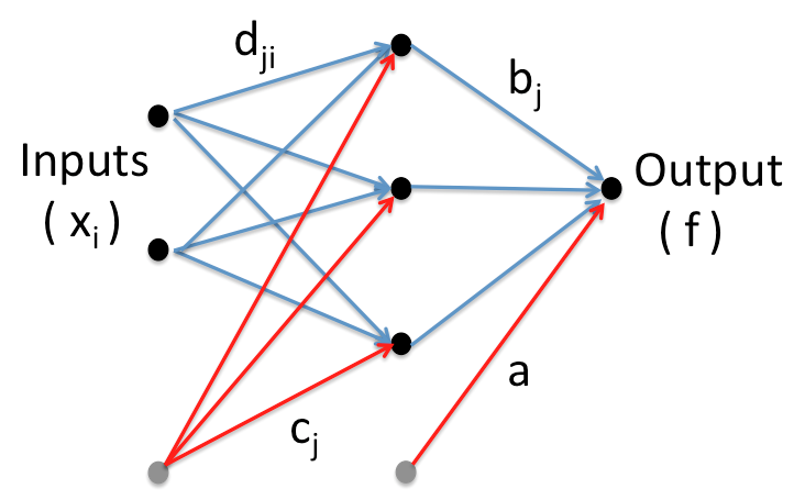
Figure 1: A feed-forward neural network with a single hidden layer, two inputs $Z$ and $A$, and a single output $f=\delta_{\textrm{LDM}}(Z,A)$.

The specification of a prior is an essential part of any Bayesian analysis. For this problem, the prior density $p(\omega)$ should encode what is known about the neural network parameters. A priori, these parameters can be positive or negative and, with the exception of parameter $a$ in Eq. (14), should be constrained to lie close to zero in order to obtain an approximation for $\delta_{\textrm{LDM}}(Z,A)$ that is as smooth as possible. We therefore follow Ref. Neal (1996) and assign a zero mean Gaussian prior for each neural network parameter, while similar parameters in Eq. (14) are assigned the same standard deviation: $\sigma_{a}$ for parameter $a$, $\sigma_{b}$ for the parameters $b_{j}$, $\sigma_{c}$ for the parameters $c_{j}$, and $\sigma_{d}$ for the parameters $d_{ji}$. However, since a priori, we do not know what values should be assigned to these standard deviations, we allow them to vary over a range by constraining the precisions ($1/\sigma^{2}$) using a prior (which is often referred to as a hyperprior, that is, a “prior that constrains a prior”) for each of the four standard deviations, each modeled as a gamma density defined by two fixed parameters Neal (1996). The fixed parameters of the gamma densities are chosen so as to maximize the accuracy of the predictions. The prior $p(\omega)$ is therefore the integral with respect to the four precisions of a product of Gaussians, one for each neural network parameter, times the four gamma densities, one for each of the precisions, $1/\sigma_{a}^{2}$, $1/\sigma_{b}^{2}$, $1/\sigma_{c}^{2}$, and $1/\sigma_{d}^{2}$.

Having laid out the foundation of the BNN method, we now proceed to construct a model of nuclear masses by training BNNs on mass residuals,

$$t(x)=M_{\rm exp}(x)-M_{\rm th}(x),$$ (15)

that is, the difference between the experimental values and the theoretical predictions from a given mass model. This strategy is consistent with the approach articulated in the Introduction: we include as much physics as possible by using the physics-motivated models in the literature and use the BNN to fine tune these models by modeling the residuals.

III Results

To illustrate the BNN approach we begin with the simplest mass model available in the literature: the liquid drop model of Bethe and Weizsäcker introduced in Eq. (2). As it is customarily done, optimal values for the six empirical parameters are determined from a least-squares fit to the experimental binding energies of the more than 3,200 nuclei listed in the latest AME2012 compilation Wang et al. (2012). Note that by implementing a MCMC-Metropolis algorithm for a likelihood function defined as in Eq.(10) Piekarewicz et al. (2015), one can obtain optimal values with associated theoretical uncertainties; see Table 1.

$a_{\rm v}$(MeV)	$a_{\rm s}$(MeV)	$a_{\rm c}$(MeV)	$a_{\rm a}$(MeV)	$a_{\rm as}$(MeV)	$a_{\rm p}$(MeV)
$15.422(17)$	$16.831(53)$	$0.686(1)$	$26.002(111)$	$-18.711(482)$	$11.199(388)$

Table 1: Liquid-drop-model parameters and uncertainties obtained from the latest AME2012 compilation of nuclear masses Wang et al. (2012).

Having defined a theoretical model one can now start with the implementation of the BNN algorithm. The training of the neural network requires a separation of the data into three different sets: (a) learning, (b) validation, and (c) prediction. The learning set consists of a randomly selected group of nuclei within the AME2012 database that will be used to sample the parameters of the neural network function given in Eq.(14). The validation set comprises nuclei that are still within the AME2012 database but that were not used in the modeling of the residual function $\delta_{\textrm{LDM}}(Z,A)$. Finally as the name suggests, the prediction set consists of a group of nuclei not contained in the AME2012 compilation but that are vital for elucidating phenomena sensitive to such (unknown) masses, as in the case of the composition of the neutron star crust.

In the spirit of Strutinsky’s energy theorem Strutinsky (1967), we assume that the liquid drop model provides—as indeed it does—an accurate description of the large and smooth behavior of the underlying mass function. Then, the BNN algorithm is used to refine the LDM predictions by modeling $\delta_{\textrm{LDM}}(Z,A)$. In the case of the LDM, the residuals represent the small deviations that are not captured by the LDM model. To avoid regions of the nuclear landscape where the masses fluctuate too rapidly (as in the case of light nuclei) or where the experimental uncertainties are large (such as for very massive nuclei), we limit our data set to the 2591 nuclei between ⁴⁰Ca and ²⁴⁰U. From this limited (yet still very large) set, the learning set is built from 1800 randomly selected nuclei (about 70% of the original set). The remaining 791 nuclei constitute the validation set. With two input variables ($Z$ and $A$) and $H\!=\!40$ hidden nodes, a total of $1\!+\!4H\!=\!161$ parameters must be sampled. To do so, we use the Flexible Bayesian Modeling package by Neal described in Ref. Neal (1996). After an initial thermalization phase consisting of 500 iterations, sampling data are accumulated for a total of 100 iterations that are used to determine statistical averages, via Eq. (12), and their associated uncertainties.

To assess the quality of the resulting neural network function $f(x,\omega)$, we compute the mean-square deviation

$$\sigma^{2}=\frac{1}{K}\sum_{k=1}^{K}\Big{[}M_{\rm exp}(k)-M_{\rm th}(k)\Big{]}^{2},$$ (16)

of the mass of the $K\!=\!290$ nuclei (out of the 791 nuclei in the validation set) that are of relevance to the composition of the outer stellar crust, namely, those spanning the $Z\!=\!20$-$50$ region. Note that in the above expression “exp” stands for the experimentally quoted value in the AME2012 compilation and “th” for the corresponding theoretical prediction. The root-mean-square deviation as per Eq. (16) for a representative set of sophisticated mass models are displayed in Table 2. These include the microscopic-macroscopic mass models of Duflo and Zuker (DZ) Duflo and Zuker (1995), Möller and Nix (MN) Möller and Nix (1981, 1988), and the finite range droplet model (FRDM) Möller et al. (1995), alongside the two accurately calibrated microscopic models HFB19 and HFB21 Goriely et al. (2010).

As shown in Table 2, for all these five mass models the root mean square deviation—denoted as $\sigma_{\rm pre}$—falls in the range of $0.5$-$1$ MeV. In contrast and consistent with expectations, the simple liquid drop model yields a deviation that is considerably larger ($\sim\!3.6\,{\rm MeV}$). However, once properly trained, the BNN-improved liquid-drop model (listed on the second line as $\sigma_{\rm post}$) rivals the predictions of the most accurate of these models. This important finding validates the basic tenet of this work, namely, that the small and fluctuating contribution to the nuclear mass may be accounted for by properly training on the residuals.

Model	LDM	DZ	MN	FRDM	HFB19	HFB21
$\sigma_{\rm pre}$ (MeV)	3.359	0.526	0.963	0.861	0.880	0.816
$\sigma_{\rm post}$ (MeV)	0.556	0.303	0.507	0.460	0.524	0.555
$\Delta\sigma/\sigma_{\rm pre}$	0.835	0.424	0.474	0.466	0.405	0.320

Table 2: Root-mean-square deviation as predicted by a representative set of models for the mass of 290 nuclei of possible relevance to the outer crust of a neutron star; see text for details.

For a graphical depiction of our findings–and with an eye on further refinements—we display in Fig. 2 predictions for the masses of the Krypton isotopes ($Z\!=\!36$) in the ^96-112Kr range. For ease of viewing, we plot the theoretical predictions relative to a reference mass. For the ^96-101Kr region where experimental masses are available, we use the AME2012 tabulated values Wang et al. (2012), whereas for the $N\!\geq\!66$ region we use the Duflo-Zuker predictions as the reference mass; this “transition” region is delineated by the dashed vertical line. Besides predictions from the five models (DZ, MN, FRDM, HFB19, and HFB21) we include BNN-improved results from the liquid drop model with associated theoretical uncertainties. Having previously validated the BNN algorithm, these predictions were made with a refined neural network function that used as the learning set all 2591 nuclei between ⁴⁰Ca and ²⁴⁰U.

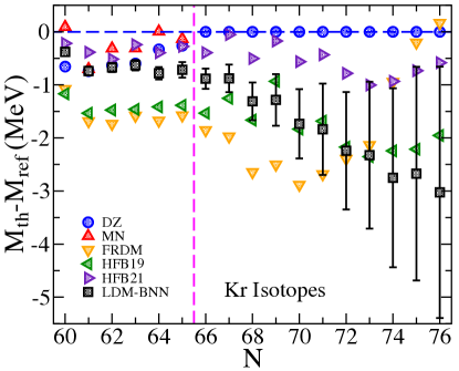
Figure 2: Mass predictions for the Krypton isotopes relative to a reference mass from all the five mass models considered in the text. Also shown are the predictions from the BNN-improved liquid drop model with its associated theoretical errors. The reference mass is taken from AME2012 for $60\!\leq\!N\!\leq\!65$ and from the Duflo-Zuker model for $N\!>\!65$.

In the $60\!\leq\!N\!\leq\!65$ region, the predictions of all the models—including the BNN improved LDM—are within 2 MeV of the experiment. Perhaps more relevant is the fact that the statistical errors associated with the LDM-BNN predictions suggest that in this region the systematic errors associated with the various models (although relatively small) dominate over the statistical uncertainties. This indicates a need for a better understanding of the sources that dominate the $\sim\!2$ MeV systematic uncertainties. In sharp contrast, the uncertainties in the $N\!>\!65$ region where no data is available are dominated by the statistical error—especially for the most neutron-rich isotopes. Without errors, one could be under the false impression that the models are inconsistent with each other. This fact underscores the critical importance of uncertainty quantification. Indeed, theoretical predictions without accompanying statistical errors—especially when large extrapolations are involved—are of very little value. Finally, our results highlight the vital role of future rare isotope facilities. Although the outer crust requires extrapolations into regions of the nuclear chart that are unlikely to be explored even with the most sophisticated rare isotope beam facilities—after all, ¹¹⁸Kr is 21 neutrons away from the last isotope with a well measured mass—mass measurements of even a few of these exotic short-lived isotopes could prove crucial in informing nuclear-structure models.

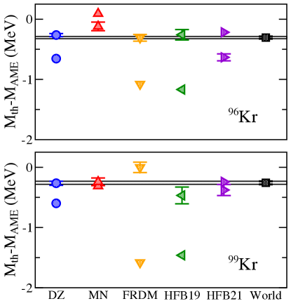
Figure 3: Pre- and post-BNN improved mass predictions relative to the AME2012 tabulated values for ⁹⁶Kr and ⁹⁹Kr. The BNN predictions include statistical errors and “World” represents the world average of the five models obtained as per Eq. (17).

Given the promise of the approach, it seems natural to extend the BNN formalism to the five high-quality mass models considered in this work. Thus, exactly as it was done in the case of the liquid-drop model, we use approximately 70% of the nuclear masses tabulated in the AME2012 compilation to train (using mass residuals) each of the five individual mass models. What emerges are five different neural network functions each with its own set of parameters. Once calibrated, we then use the same 290 nuclei (out of 791) that were used earlier to validate the LDM-BNN model to assess the quality of the BNN refinement. The resulting root-mean-square deviation $\sigma_{\rm post}$ are listed in Table 2 alongside the previously shown result for the liquid drop model. In all cases we observe a considerable improvement. This is particularly significant given that these represent some of the most sophisticated mass models available to date. This observation validates our approach of incorporating as much physics as possible into the underlying mass model but ultimately relying on an empirical BNN model to refine the mass model.

To illustrate this refinement in graphical form we display in Fig. 3 theoretical predictions for the masses of ⁹⁶Kr and ⁹⁹Kr relative to the experimental value Wang et al. (2012). As in the case of Fig. 2—and because extrapolations are unavoidable—these predictions have been done using the entire AME2012 mass compilation as the learning set. Although the pre-BNN predictions of all five models are fairly accurate, they display a significant amount of systematic variations. However, once the BNN refinement is implemented, most of these systematic differences disappear. Moreover, an estimate of uncertainty is now associated with each mass model. Ultimately, this enables us to compute a “world average” value by combining the BNN-improved predictions in the following way:

$$M_{\rm world}=\sum_{n}\omega_{n}\,M_{n}\,,\hskip 8.0ptV_{\rm world}=\sum_{n}\omega_{n}^{2}\,V_{n}\,,\hskip 4.0pt{\rm and}\hskip 6.0pt\omega_{n}=\frac{V_{n}^{-1}}{\sum_{n}V_{n}^{-1}}\,,$$ (17)

where the sum runs over all the models and $V_{n}$ represents the variance of each model. As was done in Fig. 3, we display in Fig. 4 the same trends but now for the case of the more exotic ¹⁰²Kr, ¹⁰⁵Kr, ¹⁰⁸Kr, and ¹¹¹Kr isotopes where experimental information is not yet available (also unavailable are predictions from the model by Möller-Nix). Given the lack of experimental data, the increase with $N$ of both the systematic and statistical uncertainties is hardly surprising. Again, this underscores the pressing need for measuring masses of exotic nuclei at rare isotope facilities.

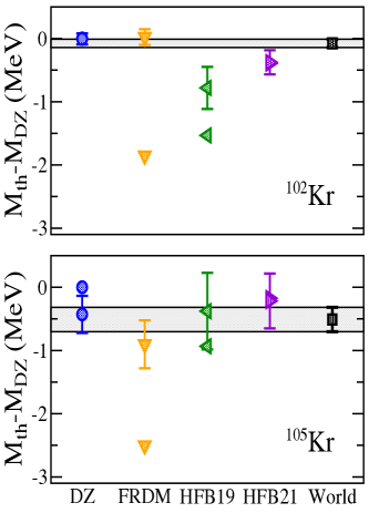
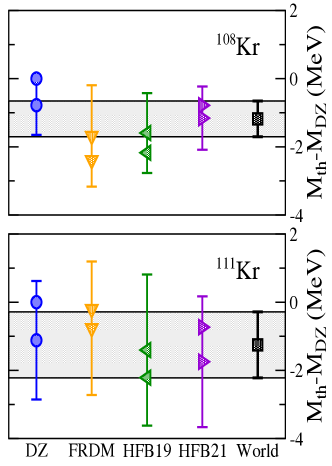
Figure 4: Pre- and post-BNN improved mass predictions relative to the “bare” Duflo-Zuker values for ¹⁰²Kr, ¹⁰⁵Kr, ¹⁰⁸Kr, and ¹¹¹Kr. The BNN predictions include statistical errors and “World” represents the world average of the four models obtained as per Eq. (17).

Having obtained a mass model—generated from the world averages as defined in Eq. (17)—we are now in a position to predict the composition of the outer stellar crust. To do so, the pressure $P(r)$ and mass $M(r)$ profiles of the star are generated via the Tolman-Oppenheimer-Volkoff (TOV) equations:

$$\frac{dP}{dr}=-G\frac{M(r)\mathcal{E}(r)}{r^{2}}\left[1+\frac{P(r)}{\mathcal{E}(r)}\right]\left[1+\frac{4\pi r^{3}P(r)}{M(r)}\right]\left[1-\frac{2GM(r)}{r}\right]^{-1},$$ (18)

$$\frac{dM}{dr}=4\pi r^{2}\mathcal{E}(r).$$ (19)

Here $\mathcal{E}(r)$ is the energy density that is connected to the pressure $P(r)$ via an equation of state. To illustrate the procedure we consider a “canonical” $M_{0}\!=\!1.4\,M_{\odot}$ neutron star with a radius of $R_{0}\!=\!12.78$ km as predicted by a realistic equation of state Todd-Rutel and Piekarewicz (2005). These two quantities are sufficient to define the boundary conditions at the edge of the outer crust, namely, $M(R_{0})\!=\!M_{0}$ and $P(R_{0})\!=\!P_{0}\!\approx\!0$. Given $P_{0}$, the corresponding baryon density, energy density, and composition may be determined from the minimization of the chemical potential; see Eqs. (4), (6), and (7). At such an infinitesimal pressure (and baryon density), the crystalline lattice is composed of ⁵⁶Fe nuclei.

Knowledge of $M_{0}$, $P_{0}$ and $\mathcal{E}_{0}\!=\!\mathcal{E}(R_{0})$ is all that is needed to integrate inward the TOV equations to determine both the pressure and enclosed mass at the next (interior) point. With such pressure at hand, one proceeds once more to determine the associated baryon density, energy density, and composition at the given depth. This allows one to integrate inward the TOV equations to the next point, and so on. This iterative procedure continues until the total chemical potential of the system becomes equal to the free neutron mass. At this density it is no longer possible to bind all the neutrons into nuclei; the “neutron drip line” is reached. This stellar depth demarcates the transition from the outer to the inner crust.

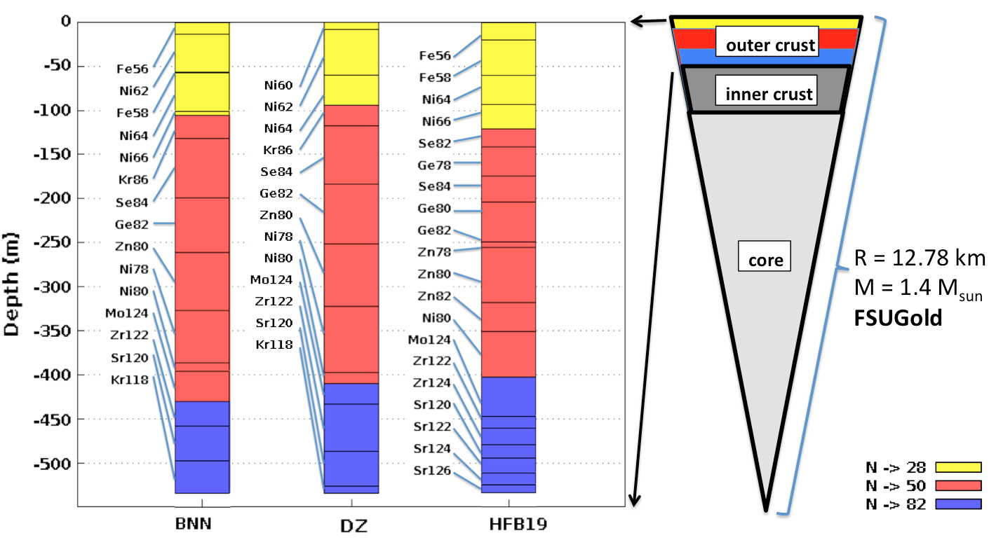
Figure 5: Composition of a canonical $1.4\,M_{\odot}$ neutron star with a 12.78 km radius as predicted by three mass models: “BNN-world”, DZ, and HFB19.

In Fig. 5 we display the composition of the outer crust as a function of depth for a neutron star with a mass of $1.4\,M_{\odot}$ and a radius of 12.78 km. Predictions are shown using our newly created mass model “BNN-world”, Duflo Zuker, and HFB19; these last two without any BNN refinement. The composition of the upper layers of the crust (spanning about 100 m and depicted in yellow) consists of Fe-Ni nuclei with masses that are well known experimentally. As the Ni-isotopes become progressively more neutron rich, it becomes energetically favorable to transition into the magic $N\!=\!50$ isotone region. In the particular case of BNN-world, this intermediate region is predicted to start with stable ⁸⁶Kr and then progressively evolve into the more exotic isotones ⁸⁴Se ($Z\!=\!34$), ⁸²Ge ($Z\!=\!32$), ⁸⁰Zn ($Z\!=\!30$), and ⁷⁸Ni ($Z\!=\!28$); all this in an effort to reduce the electron fraction. In this region, most of the masses are experimentally known, although for some of them the quoted value is not derived from purely experimental data Wang et al. (2012). Ultimately, it becomes energetically favorable for the system to transition into the magic $N\!=\!82$ isotone region. In this region none of the relevant nuclei have experimentally determined masses. Although not shown, it is interesting to note that the composition of the HFB19 model changes considerably after the BNN refinement, bringing it into closer agreement with the predictions of both BNN-world and Duflo-Zuker. Although beyond the scope of this work, we should mention that the crustal composition is vital in the study of certain elastic properties of the crust, such as its shear modulus and breaking strain—quantities that are of great relevance to magnetar starquakes Piro (2005); Steiner and Watts (2009) and gravitational wave emission Horowitz and Kadau (2009).

IV Conclusions

The determination of nuclear masses lies at the core of Nuclear Physics. Starting almost eight decades ago with the pioneering work of Bethe and Weizsäcker and continuing to this day with the development of ever more sophisticated theoretical models, the prediction of nuclear masses is not only of great intrinsic interest but, in addition, plays a fundamental role in elucidating a variety of astrophysical phenomena. However, despite the sophistication and success of modern mass models, systematic uncertainties associated with the constraints and limitations of each model remain. Moreover, these systematic uncertainties continue to grow as the models are extrapolated to uncharted regions of the nuclear landscape. Given that mass-sensitive astrophysical phenomena, such as r-process nucleosynthesis and the composition of the neutron star crust, demand knowledge of nuclear masses far away from stability, it becomes imperative to reconcile some of these differences. In this work we have introduced a novel approach firmly rooted in Strutinsky’s energy theorem that suggests that the nuclear binding energy may be separated into a large and smooth component and another one that is small and fluctuating. Using the liquid drop model as an example to generate the large and smooth component, we then invoked a Bayesian neural network approach to account for the small and fluctuating component of the binding energy. The BNN formalism is an approximation method that relies on the application of Bayes’ theorem and a highly non-linear neural network function. By doing so, we obtained a refined LDM that rivals the predictions of the most sophisticated mass models available to date.

Motivated by the success of the BNN approach, we have extended the formalism to five of the most successful mass models available in the literature. The aim was to overcome the unavoidable limitations of any model by building an artificial neural network function that could account for the small deviations from experiment. Moreover, due to the probabilistic nature of the Bayesian approach, the improved predictions were now accompanied by proper theoretical errors. Despite the undeniable quality of the original mass models, significant improvements were observed in all cases after the implementation of the BNN protocol. As important, the spread among the various models was considerable reduced. Ultimately, a new mass model was obtained by combining the various model predictions (after BNN refinement) into a “world average”.

As a first test of the new mass model we have computed the composition of the outer crust of a neutron star, as it is only sensitive to nuclear masses in the $20\!\lesssim\!Z\!\lesssim\!50$ range. Whereas the composition in the upper layers of the crust is model independent, the situation is drastically different in the high density layers where the models predict a composition that is unlikely to ever be recreated in the laboratory. Indeed, the exotic nucleus of ¹¹⁸Kr—21 neutrons removed from the last isotope with a well measured mass—is predicted to lie at the very bottom layer of the outer crust. Although mass measurements of some of these exotic $N\!=\!82$ isotones (such as ¹¹⁸Kr, ¹²⁰Sr, ¹²²Zr, and ¹²⁴Mo) may not be feasible even at future state-of-the-art facilities, it is critical to continue this quest as far as possible from stability to properly inform theoretical models.

The study of the composition of the stellar crust represents a proof-of-principle implementation of the BNN protocol to the important case of nuclear masses. However, this relatively simple example represents the “tip of the iceberg”. For example, the newly created mass model may also be used to compute neutron separation energies for the neutron-rich isotopes of relevance to r-process nucleosynthesis. Moreover, the BNN framework is flexible and powerful enough to be extended to other physical observables. The basic requirement is the existence of a robust theoretical model with a strong physics underpinning, so that the residuals between theory and experiment become a smooth function of the input parameters (e.g., $Z$ and $A$). In that case, such a smooth function could be accurately represented by an artificial neural network function. Natural extensions of the BNN approach to other nuclear observables with already large experimental databases are charge radii and beta-decay lifetimes, among others. Work along these lines is currently in progress.