Recovery of Sparse Positive Signals on the Sphere from Low Resolution Measurements

Abstract

This letter considers the problem of recovering a positive stream of Diracs on a sphere from its projection onto the space of low-degree spherical harmonics, namely, from its low-resolution version. We suggest recovering the Diracs via a tractable convex optimization problem. The resulting recovery error is proportional to the noise level and depends on the density of the Diracs. We validate the theory by numerical experiments.

I Introduction

Many applications in engineering and physics consider signals that lie on spheres (see for instance, [3, 23, 27, 22]). In this letter we consider the problem of recovering a positive stream of Diracs on the sphere from its low-resolution measurement. The natural way to model a low-resolution version of a signal on a sphere is by its projection onto the space of low-degree spherical harmonics, as will be explained in Section II.

This work is motivated by the problem of estimating the orientations of the white matter fibers in the brain using diffusion weighted magnetic resonance imaging (MRI) [24]. It is common to model the measured signal as a spherical convolution of the underlying distribution of fiber bundles, called the orientation density function, with the point spread function of the diffusion tensor imaging sequence which smears out the fine details of the fibers’ distribution. The orientation density function is modeled as a stream of Diracs on the sphere. The locations and the positive weights of the Diracs represent the orientations of the fibers and the partial volume of the fiber within a voxel, respectively [32, 17]. Therefore, the mathematical model elaborated in Section II suits this application.

From the theoretical side, as far as we know, this is the first work to suggest a stable recovery of positive signals on the sphere from their low-resolution measurements. This result is part of an ongoing effort to derive recovery guarantees for super-resolution of signals in various geometries and settings (see, e.g. [10, 11, 12, 20, 28, 16, 7, 8, 5, 6]).

Several papers considered the recovery of Diracs on a sphere with general coefficients (not necessarily positive) from their low-resolution measurements. In [6, 9] it was shown that recovery via convex optimization methods is robust under the assumption that the Diracs are sufficiently separated (see Theorem II.2). The papers [18, 19] employ a finite rate of innovation framework to super-resolve Diracs on the sphere. This approach does not need any assumption on the Diracs’ distribution. However, these works have no robustness guarantees. Additionally, in [9] it was proven that separation is necessary for robust recovery in the presence of noise by any method.

Following [29], we show that if the Diracs are known to be positive then the separation condition can be replaced by a weaker condition called Rayleigh regularity, which quantifies the density of the Diracs. We suggest recovering the Diracs via a tractable convex optimization problem. The resulting recovery error is proportional to the noise level and depends on the Rayleigh regularity of the signal.

The letter is organized as follows. In Section II we formulate the problem and present necessary mathematical background. Section III presents our main result, which is proved in Section IV. Section V shows some numerical experiments, which corroborate the theoretical results, and Section VI concludes the letter.

II Problem Formulation and Background

Spherical harmonics play a key role in the analysis of signals in a vast variety of tasks, analysis methods and sampling theorems, see for instance; [1, 31, 14, 26, 25, 21]. Let $\mathcal{Y}_{n}\left(\mathbb{S}^{2}\right)$ denote the space of homogeneous spherical harmonics of degree $n$, which is the restriction to the bivariate unit sphere of the homogeneous harmonic polynomials of degree $n$ in $\mathbb{R}^{3}$.

Any point on the bivariate unit sphere $\mathbb{S}^{2}$ is parametrized by $x:=\left(\phi,\theta\right)\in[0,2\pi)\times\left[0,\pi\right]$. The distance between two points $x_{i},x_{j}\in\mathbb{S}^{2}$ is measured as

$$\rho\left(x_{i},x_{j}\right):=\arccos\left(x_{i}\cdot x_{j}\right).$$ (II.1)

Let

$$Y_{n,k}=A_{n,k}e^{jk\phi}P_{n,k}\left(\cos\theta\right),\quad k=-n,\dots,n,$$

be an orthonormal basis of $\mathcal{Y}_{n}\left(\mathbb{S}^{2}\right)$, where $P_{n,k}\left(x\right)$ is an associated Legendre polynomial of degree $n$ and order $k$, and

$$A_{n,k}:=\sqrt{\frac{2n+1}{4\pi}\frac{\left(n-\left|k\right|\right)!}{\left(n+\left|k\right|\right)!}}.$$

The functions $\left\{Y_{n,k}\right\}$ are the eigenfunctions of the Laplacian on $\mathbb{S}^{2}$, and thus can be understood as the extension of Fourier analysis on the sphere. Any function $g\in L_{2}\left(\mathbb{S}^{2}\right)$ can be expanded as [2]

$$g(x)=\sum_{n=0}^{\infty}\sum_{k=-n}^{n}\left\langle g,Y_{n,k}\right\rangle Y_{n,k}(x).$$

In this work, we consider a discrete positive signal of the form

$$f[x]=\sum_{m=1}^{M}c_{m}\delta\left[x-x_{m}\right],\quad c_{m}>0,$$ (II.2)

where $\delta\left[x\right]$ is the Kronecker delta function and $X:=\left\{x_{m}\right\}$ is the signal’s support. We assume that the signal lies on some predefined grid $\mathbb{S}_{L}^{2}\subset\mathbb{S}^{2}$ and that any pair of points on the grid $x_{i},x_{j}\in\mathbb{S}_{L}^{2}$ satisfy $\rho\left(x_{i},x_{j}\right)\geq 1/L$ for some $L\geq 1/\pi$. The higher $L$ is, the larger the target resolution we want to achieve.

The information we have on the signal is its projection onto the space of the low $N$ spherical harmonics

$$\begin{split}&y_{n,k}=\left\langle f,Y_{n,k}\right\rangle+\eta_{n,k},\\ &n=0,\dots,N,\quad k=-n,\dots,n,\end{split}$$ (II.3)

where $\eta:=\left\{\eta_{n,k}\right\}$ is some noise or model mismatch which is assumed to be bounded. In matrix notation we may write

$$y=F_{N}f+\eta\iff s:=F_{N}^{*}y=P_{N}f+F_{N}^{*}\eta,$$ (II.4)

where $y:=\left\{y_{n,k}\right\}$, $F_{N}$ is a linear operator mapping a signal to its low $N$ spherical harmonic coefficients, and the adjoint operator is given by $F_{N}^{*}z(x)=\sum_{n\leq N,\left|k\right|\leq n}z_{n,k}Y_{n,k}(x).$ The operator $P_{N}=F_{N}^{*}F_{N}$ is the orthogonal projection onto the space of spherical harmonics of degree $N$, denoted by $V_{N}$. We aim to recover the sets $\left\{c_{m}\right\},\thinspace\left\{x_{m}\right\}$ from the noisy low-resolution measurements (II.3).

In recent papers [6, 9], it was shown that signals of the form (II.2) with general coefficients (namely, not necessarily positive values) can be recovered robustly from $V_{N}$ by solving a tractable convex program. This holds provided that the signal’s support $X$ satisfies the following separation condition:

Definition II.1.

A set of points $X\subset\mathbb{S}^{2}$ is said to satisfy the minimal separation condition if

$$\min_{x_{i},x_{j}\in X,\thinspace i\neq j}\rho\left(x_{i},x_{j}\right)\geq\frac{\nu}{N},$$

for a fixed separation constant $\nu$ that does not depend on $N$, where $\rho$ is defined in (II.1).

We will also make use of the notion of the super-resolution factor (SRF). The SRF quantifies the ratio between the resolution we want to achieve, specified by the grid spacing $1/L$, and the resolution we measure, namely,

$$SRF:=\frac{L}{N}.$$ (II.5)

The main result of [9] then states the following:

Theorem II.2.

Let $X=\left\{x_{m}\right\}\subset\mathbb{S}_{L}^{2}$ be the support of a signal of the form (II.2) with general coefficients $c_{m}\in\mathbb{R}$. Let $\left\{y_{n,k}\right\}$ be as in (II.3) with $\left\|\eta\right\|_{\ell_{2}}\leq\delta$. For sufficiently large $L$, if $X$ satisfies the separation condition of Definition II.1, then the solution $\hat{f}$ of

$$\min_{g\in\mathbb{S}_{L}^{2}}\left\|g\right\|_{\ell_{1}}\mbox{ subject to }\left\|y-F_{N}g\right\|_{\ell_{2}}\leq\delta,$$ (II.6)

satisfies

$$\left\|\hat{f}-f\right\|_{\ell_{1}}\leq C_{0}SRF^{2}\delta,$$

for some fixed constant $C_{0}$.

Remark II.3.

The minimal separation constant $\nu$ was evaluated numerically to be $2\pi$. The separation of $\frac{2\pi}{N}$ coincides with the spatial resolution of signals on spheres [30].

The aim of this letter is to derive a stability result for the recovery of positive signals on the sphere from their low-resolution measurements. In this case, as presented in the next section, the separation condition can be replaced by a weaker condition called Rayleigh regularity.

III Main result

In [6], it was proven that a positive signal on the sphere with $M\leq N/2$ (i.e. maximal cardinality of $N/2$) can be perfectly recovered from its noiseless projection onto $V_{N}$ by solving a convex optimization problem. A general signal of cardinality $M$ can be recovered from $V_{M+1+\sqrt{M+1}}$ by an algebraic approach [19]. However, both recovery results are not stable in the presence of noise.

To derive a stability result for the positive case, we use the notion of Rayleigh regularity. A univariate signal with Rayleigh regularity $r$ has at most $r$ spikes within a resolution cell of size $\frac{\mu}{N}$ for a separation constant $\mu$. In the multidimensional case, the definition of Rayleigh regularity is less intuitive (see discussion in [4]) and can be interpreted as a density measure of the signal. For $r=1$, the definition coincides with Definition II.1.

Definition III.1.

We say that the set $\mathcal{P}\subset\mathbb{S}_{L}^{2}$ is Rayleigh-regular with parameters $(\mu,r\thinspace;\thinspace N,L)$ and write $\mathcal{P}\in\mathcal{R}^{idx}(\mu,r\thinspace;\thinspace N,L)$ if

• $\mathcal{P}\mathcal{=}\mathcal{P}_{1}\cup\dots\cup\mathcal{P}_{r}$ and $\mathcal{P}_{i}\cap\mathcal{P}_{j}=\emptyset$ for all $i\neq j$,

• for all $i=1,\dots,r,$ $\mathcal{P}_{i}$ satisfies the separation condition of Definition II.1 with constant $\mu$.

We denote the set of positive signals of the form (II.2) with support $X\in\mathcal{R}^{idx}(\mu,r\thinspace;\thinspace N,L)$ as $\mathcal{R}_{+}(\mu,r\thinspace;\thinspace N,L)$.

The notion of Rayleigh regularity was used in [29] to derive stability results for the recovery of positive signals from their low-degree Fourier coefficients. Our results can be seen as an extension to signals on spheres.

In the sequel, we assume that the noise satisfies $\left\|F_{N}^{*}\eta\right\|_{\ell_{1}}\leq\delta$ and suggest to recover the signal by solving the feasibility (convex) problem

$$\mbox{find }g\in\mathbb{S}_{L}^{2}\quad\mbox{subject to}\quad\left\|s-P_{N}g\right\|_{\ell_{1}}\leq\delta,\thinspace g\geq 0.$$ (III.1)

Now, we are ready to present our main theorem. The theorem states that by solving the convex program (III.1), one can stably recover a positive signal on the sphere from its low-resolution measurements. The recovery error is proportional to the noise level and depends on the Rayleigh regularity of the signal.

Theorem III.2.

Let $f\in\mathcal{R}_{+}(\nu r,r\thinspace;\thinspace N,L)$ be of the form (II.2) and consider the measurement model (II.3). Then, for sufficiently large SRF, any solution $\hat{f}$ of (III.1) satisfies

$$\left\|\hat{f}-f\right\|_{\ell_{1}}\leq 4C_{1}^{-r}r^{2r}SRF^{2r}\delta,$$

for some fixed constant $C_{1}>0$.

Corollary III.3.

In the noiseless case, $\delta=0$, the recovery is exact.

As we show in the simulations, minimizing the $\ell_{1}$ norm in (III.1) among all feasible solutions results in a low recovery error.

IV Proof of Theorem III.2

The proof exploits the technique presented in [29] (see also [4]). We commence by presenting the following Lemma which is a direct consequence of the construction in [6]:

Lemma IV.1.

Suppose that the set $\Xi=\left\{\xi_{m}\right\}\subset\mathbb{S}^{2}$ satisfies the separation condition of Definition II.1. Then, for sufficiently large $N$ there exists a polynomial $q\in V_{N}$ obeying $q(\xi)\leq 1$ and

$$q\left(\xi_{m}\right) = 0,\quad\forall\xi_{m}\in\Xi,$$

$$q\left(\xi\right) \geq C_{1}N^{2}\rho\left(\xi,\xi_{m}\right)^{2},\quad\rho\left(\xi,\xi_{m}\right)\leq\sigma/N,\thinspace\xi_{m}\in\Xi,$$

$$q\left(\xi\right) \geq C_{2},\quad\mbox{if }\rho\left(\xi,\xi_{m}\right)>\sigma/N\mbox{,\thinspace$\forall$$\xi_{m}\in\Xi$},$$

for constants $\sigma,C_{1}>0$ and $0<C_{2}<1$.

Set $h:=\hat{f}-f\subset\mathbb{S}_{L}^{2}$ where $\hat{f}$ is the solution of the convex program (III.1). Let $\mathcal{H}:=\left\{x\in\mathbb{S}_{L}^{2}\thinspace:\thinspace h\left[x\right]<0\right\}$ and thus $\mathcal{H}\subseteq X$. By assumption $f\in\mathcal{R}_{+}(\nu r,r\thinspace;\thinspace N,L)$ and consequently $\mathcal{H}\in\mathcal{R}^{idx}(\nu r,r\thinspace;\thinspace N,L)$. Therefore, by Definition III.1, the set $\mathcal{H}$ can be presented as a disjoint union of $r$ sets $\mathcal{H}=\cup_{i=1}^{r}\mathcal{H}_{i},$ where $\mathcal{H}_{i}\in\mathcal{R}^{idx}(\nu r,1\thinspace;\thinspace N,L)$ for all $i=1,\dots,r$. Observe that by simple rescaling $\tilde{N}=N/r$ we have

$$\mathcal{R}^{idx}(\nu r,1\thinspace;\thinspace N,L)=\mathcal{R}^{idx}(\nu,1\thinspace;\thinspace N/r,L).$$

Then, for each set $\mathcal{H}_{i}$ there exists an associated interpolating polynomial $q_{i}(x)\in V_{N/r}$ as given in Lemma IV.1.

The key ingredient of the proof is the following construction:

$$\grave{q}\left(x\right)=\prod_{i=1}^{r}q_{i}\left(x\right)-\alpha,$$

where $\alpha>0$ is a constant to be determined later. A product of spherical harmonics of degrees $N_{1},N_{2}$ is a spherical harmonic of degree $N_{1}+N_{2}$ and the computation of the corresponding representation is known as Clebsch-Gordan. Therefore, $\grave{q}\in V_{N}.$ We denote by $\grave{q}_{L}[x]$ the restriction of $\grave{q}(x)$ to the grid $\mathbb{S}_{L}^{2}$.

By construction, for all $x\in\mathcal{H}$ we have $q_{i}\left(x\right)=0$ for some $i=1,\dots,r$. Therefore,

$$\grave{q}_{L}\left[x\right]=\prod_{i=1}^{r}q_{i}\left(x\right)-\alpha=-\alpha.$$

Additionally, for sufficiently large SRF (see (II.5)) we get that for all $x\in\mathbb{S}_{L}^{2}\backslash\mathcal{H}$,

$$\grave{q}_{L}\left[x\right] \geq C_{1}^{r}L^{-2r}\left(\frac{N}{r}\right)^{2r}-\alpha$$

$$= C_{1}^{r}r^{-2r}SRF^{-2r}-\alpha.$$

By setting

$$\alpha:=\frac{1}{2}C_{1}^{r}r^{-2r}SRF^{-2r}<1/2,$$ (IV.1)

we conclude that

$$\grave{q}_{L}\left[x\right] = -\alpha\quad\forall x\in\mathcal{H},$$ (IV.2)

$$\grave{q}_{L}\left[x\right] \geq \alpha,\quad\forall x\in\mathbb{S}_{L}^{2}\backslash\mathcal{H}.$$

Once we have constructed the appropriate polynomial $\grave{q}_{L}$, the rest of the proof follows directly. On the one hand, by (II.4) and (III.1) we get

$$\left|\left\langle\grave{q}_{L},h\right\rangle\right| = \left|\left\langle P_{N}\grave{q}_{L},h\right\rangle\right|$$

$$= \left|\left\langle\grave{q}_{L},P_{N}h\right\rangle\right|$$

$$\leq \left\|\grave{q}_{L}\right\|_{\ell_{\infty}}\left\|P_{N}\left(\hat{f}-f\right)\right\|_{\ell_{1}}$$

$$\leq \left\|\grave{q}_{L}\right\|_{\ell_{\infty}}\left(\left\|P_{N}\hat{f}-s\right\|_{\ell_{1}}+\left\|s-P_{N}f\right\|_{\ell_{1}}\right)$$

$$\leq 2\delta.$$

On the other hand, combining (IV.2) with the fact that $\grave{q}_{L}$ and $h$ have the same sign pattern on $\mathbb{S}_{L}^{2}$ we have

$$\left|\left\langle\grave{q}_{L},h\right\rangle\right| = \left|\sum_{x\in\mathbb{S}_{L}^{2}}\grave{q}_{L}[x]h[x]\right|$$

$$= \sum_{x\in\mathbb{S}_{L}^{2}}\left|\grave{q}_{L}[x]\right|\left|h[x]\right|$$

$$\geq \alpha\left\|h\right\|_{\ell_{1}}.$$

Combining (IV),(IV) and (IV.1) we conclude that

$$\left\|h\right\|_{\ell_{1}} \leq \frac{2\delta}{\alpha}$$

$$= 4C_{1}^{-r}r^{2r}SRF^{2r}\delta.$$

V Numerical experiments

We now verify the theoretical results of this paper via numerical experiments. The convex optimization problems were solved using CVX [15]. In all experiments, we set the separation constant $\nu$ to be $\frac{5\pi}{2}$ and chose a uniform grid

$$\mathbb{S}_{L}^{2}:=\left\{\left(\frac{2\pi q}{L},\frac{\pi p}{L}\right)\thinspace:\thinspace\left(q,p\right)\subset\left[0,\dots,L-1\right]^{2}\right\}.$$

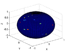
(a) The underlying signal.

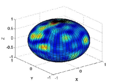
(b) Noisy measurements.

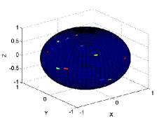
(c) The recovered signal.

Figure V.1: An example for the recovery of a signal on the sphere from its projection onto $V_{N}$ with parameters $L=60,\thinspace N=15,$ SRF=4, $r=3,M=41$ and SNR=30 db.

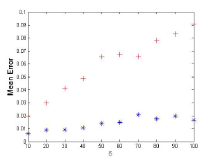
Figure V.2: The mean $\ell_{1}$ recovery error (over 10 experiments) as a function of the noise level with parameters $N=12,\thinspace L=50$ and $r=2$. The blue asterisks and the red crosses represent the recovery error with and without minimizing the $\ell_{1}$ norm among all solutions of (III.1), respectively.

Rayleigh regularity	$r=1$	$r=2$	$r=3$	$r=4$
Mean recovery error	0.0026	0.0148	0.0285	0.0584
Max recovery error	0.0059	0.0365	0.0452	0.0699

Table V.1: Mean $\ell_{1}$ recovery error (over 10 experiments for each value) of the solutions of (III.1) with minimal $\ell_{1}$ norm as a function of the signal’s Rayleigh regularity with the parameters $L=50,\thinspace N=12,\thinspace SRF\thickapprox 4$ and SNR=30 db.

The signal support was generated as a union of $r$ disjoint sets that were drawn randomly on the sphere, while keeping the separation requirements of Definition III.1. For each support location, an associated amplitude was drawn randomly from a uniform distribution on the interval $(0,10]$. Then, we computed the projection of the signal onto $V_{N}$ and added an iid normal additive noise.

We solved the feasibility convex program (III.1) and chose the solution with minimal $\ell_{1}$ norm over all feasible solutions. Figure V.1 presents a recovery example of a signal with Rayleigh regularity of $r=3$ and $M=41$ in a noisy environment of $SNR=30$ db. In Figure V.2 we compare the output of the CVX program as a function of the noise level, with and without minimizing the $\ell_{1}$ norm among all feasible solutions. The recovery error was computed as the normalized $\ell_{1}$ error, i.e.

$$\mbox{error}=\frac{1}{L^{2}}\sum_{p,q=1}^{L}\left|\hat{f}[q,p]-f[q,p]\right|.$$

Table V.1 shows the mean recovery error as a function of the Rayleigh regularity parameter $r$ with $SNR=30$ and $SRF\cong 4$.

VI Conclusion

In this letter, we proved that a discrete positive stream of Diracs on a sphere can be recovered robustly from its low-resolution measurements by solving a tractable convex optimization problem. The recovery error is proportional to the noise level and depends on the distribution of the Diracs on the sphere.

In practice, signals that have sparse representation in a continuous dictionary might not have sparse representation after discretization [13]. An obvious technique to alleviate this basis mismatch is by fine discretization, which will increase the recovery error significantly according to Theorem III.2. Proving a version of Theorem III.2 for continuous signals is therefore an important extension for future work.

References

- [1] S. Arridge. Optical tomography in medical imaging. Inverse problems, 15(2):R41, 1999.
- [2] K. Atkinsonl and W. Han. Spherical harmonics and approximations on the unit sphere: an introduction, volume 2044. Springer Science & Business Media, 2012.
- [3] P. Audet. Directional wavelet analysis on the sphere: Application to gravity and topography of the terrestrial planets. Journal of Geophysical Research: Planets (1991–2012), 116(E1), 2011.
- [4] T. Bendory. Robust recovery of positive stream of pulses. arXiv preprint arXiv:1503.08782, 2015.
- [5] T. Bendory, A. Bar-Zion, D. Adam, S. Dekel, and A. Feuer. Stable support recovery of stream of pulses with application to ultrasound imaging. arXiv preprint arXiv:1507.07256, 2015.
- [6] T. Bendory, S. Dekel, and A. Feuer. Exact recovery of dirac ensembles from the projection onto spaces of spherical harmonics. Constructive Approximation, to appear.
- [7] T. Bendory, S. Dekel, and A. Feuer. Exact recovery of non-uniform splines from the projection onto spaces of algebraic polynomials. Journal of Approximation Theory, 182:7–17, 2014.
- [8] T. Bendory, S. Dekel, and A. Feuer. Robust recovery of stream of pulses using convex optimization. arXiv preprint arXiv:1412.3262, 2014.
- [9] T. Bendory, S. Dekel, and A. Feuer. Super-resolution on the sphere using convex optimization. Signal Processing, IEEE Transactions on, 63(9):2253–2262, May 2015.
- [10] E. Candès and C. Fernandez-Granda. Towards a mathematical theory of super-resolution. Communications on Pure and Applied Mathematics, 67(6):906–956, 2014.
- [11] E.J Candès and C. Fernandez-Granda. Super-resolution from noisy data. Journal of Fourier Analysis and Applications, 19(6):1229–1254, 2013.
- [12] Y. De Castro and F. Gamboa. Exact reconstruction using beurling minimal extrapolation. Journal of Mathematical Analysis and applications, 395(1):336–354, 2012.
- [13] Y Chi, L.L Scharf, A Pezeshki, and A.R Calderbank. Sensitivity to basis mismatch in compressed sensing. Signal Processing, IEEE Transactions on, 59(5):2182–2195, 2011.
- [14] C. Cohen-Tannoudji, B. Diu, F. Laloe, and B. Dui. Quantum Mechanics (2 vol. set). Wiley-Interscience, 2006.
- [15] Inc. CVX Research. CVX: Matlab software for disciplined convex programming, version 2.0, August 2012.
- [16] L. Demanet and N. Nguyen. The recoverability limit for superresolution via sparsity. arXiv preprint arXiv:1502.01385, 2015.
- [17] S. Deslauriers-Gauthier and P. Marziliano. Spherical finite rate of innovation theory for the recovery of fiber orientations. In Engineering in Medicine and Biology Society (EMBC), 2012 Annual International Conference of the IEEE, pages 2294–2297. IEEE, 2012.
- [18] S. Deslauriers-Gauthier and P. Marziliano. Sampling signals with a finite rate of innovation on the sphere. Signal Processing, IEEE Transactions on, 61(18):4552–4561, 2013.
- [19] I. Dokmanic and Y.M. Lu. Sampling sparse signals on the sphere: Algorithms and applications. arXiv preprint arXiv:1502.07577, 2015.
- [20] V. Duval and G. Peyré. Exact support recovery for sparse spikes deconvolution. Foundations of Computational Mathematics, pages 1–41, 2013.
- [21] I Iglewska-Nowak. Continuous wavelet transforms on n-dimensional spheres. Applied and Computational Harmonic Analysis, 2014.
- [22] D. Jarrett, E. Habets, and P. Naylor. 3d source localization in the spherical harmonic domain using a pseudointensity vector. In Proc. European Signal Processing Conf.(EUSIPCO), Aalborg, Denmark, pages 442–446, 2010.
- [23] E. Komatsu, KM Smith, J Dunkley, CL Bennett, B Gold, G Hinshaw, N Jarosik, D Larson, MR Nolta, L Page, et al. Seven-year wilkinson microwave anisotropy probe (wmap) observations: cosmological interpretation. The Astrophysical Journal Supplement Series, 192(2):18, 2011.
- [24] M. Lazar, T. Bendory, Y.C Eldar, and A. Tal. Improvements in magnetic resonance tractography using spherical deconvolution of positive signals. in preparation.
- [25] B. Leistedt and J. McEwen. Exact wavelets on the ball. Signal Processing, IEEE Transactions on, 60(12):6257–6269, 2012.
- [26] J. McEwen and Y. Wiaux. A novel sampling theorem on the sphere. Signal Processing, IEEE Transactions on, 59(12):5876–5887, 2011.
- [27] J. Meyer. Beamforming for a circular microphone array mounted on spherically shaped objects. The Journal of the Acoustical Society of America, 109(1):185–193, 2001.
- [28] A. Moitra. The threshold for super-resolution via extremal functions. arXiv preprint arXiv:1408.1681, 2014.
- [29] Veniamin I Morgenshtern and Emmanuel J Candes. Super-resolution of positive sources: the discrete setup. arXiv preprint arXiv:1504.00717, 2015.
- [30] B. Rafaely. Plane-wave decomposition of the sound field on a sphere by spherical convolution. The Journal of the Acoustical Society of America, 116(4):2149–2157, 2004.
- [31] B. Rafaely. Analysis and design of spherical microphone arrays. Speech and Audio Processing, IEEE Transactions on, 13(1):135–143, 2005.
- [32] J.D. Tournier, F. Calamante, D. Gadian, and A. Connelly. Direct estimation of the fiber orientation density function from diffusion-weighted mri data using spherical deconvolution. NeuroImage, 23(3):1176–1185, 2004.