Gradient-based explanations for Gaussian Process regression and classification models

Abstract

Gaussian Processes (GPs) have proven themselves as a reliable and effective method in probabilistic Machine Learning. Thanks to recent and current advances, modeling complex data with GPs is becoming more and more feasible. Thus, these types of models are, nowadays, an interesting alternative to Neural and Deep Learning methods, which are arguably the current state-of-the-art in Machine Learning. For the latter, we see an increasing interest in so-called explainable approaches - in essence methods that aim to make a Machine Learning model’s decision process transparent to humans. Such methods are particularly needed when illogical or biased reasoning can lead to actual disadvantageous consequences for humans. Ideally, explainable Machine Learning should help detect such flaws in a model and aid a subsequent debugging process. One active line of research in Machine Learning explainability are gradient-based methods, which have been successfully applied to complex neural networks. Given that GPs are closed under differentiation, gradient-based explainability for GPs appears as a promising field of research. This paper is primarily focused on explaining GP classifiers via gradients where, contrary to GP regression, derivative GPs are not straightforward to obtain.

Keywords Gaussian Processes  $\cdot$ Explainable Machine Learning  $\cdot$ Integrated Gradients

1 Introduction

With nowadays’ widespread adoption of Machine Learning in a multitude of practical use-cases, the necessity for transparent models and algorithms is receiving more and more attention. Although complex black-box models have proven themselves to be highly performant, concerns about the consistency of their implicit, internal reasoning process is still posing a challenge. Issues in regards to fairness, representativeness or safety are commonly voiced problems that ought to be tackled by transparency improvements for complex models. Hence, the field of explainable Machine Learning has become an important and popular field of research.

Over the course of the last years, a large body of methodology has been developed to tackle the transparency issue from different angles. One promising and already successful direction can be summarized as gradient-based explainability approaches. These methods typically use the partial derivatives of a model’s output with respect to its inputs as a way to describe the relevance of each individual input feature. Although this restricts the range of Machine Learning models that benefit from this approach to end-to-end differentiable ones, many if not most of today’s popular algorithms fulfill this requirement.

Gaussian Process models (GP) on the other hand are historically seen as providing at least some sense of transparency. Most of the commonly used kernel functions for GPs induce well-known functional properties for the resulting GP. Hence, by crafting a suitable covariance kernel function, it is possible provide a sense of transparency that is often sufficient for many problems.

Problem. For more complex data like images, the sense of transparency provided by the kernel function alone might not suffice. Transparency often implies the ability to tell which features contributed to a decision for a given input. However, this is difficult to achieve with GP models that are able to actually handle such data. Thus, it is necessary to develop transparency approaches for GPs that are capable of doing so in order to mitigate potential bias and fairness issues as mentioned above.

Contribution. Gradient-based explainability is an active and considerably successful line of research that has produced remarkable results in regards to model transparency. Given the well known relation between GPs and their derivative processes, gradient-based explainability appears to be a promising candidate for transparency in complex GP models. As it turns out, gradient-based explainability is straightforward to derive for GP regression models. Classification GPs, on the other hand, do not permit a similarly simple application. Hence, this paper puts emphasis on the latter case and derives means to apply gradient explanations to the classification case as well.

Related work. In general, GPs already provide a sense of transparency that goes beyond other popular algorithms like Neural Network models. As for existing means for transparency in GPs, we can broadly distinguish two perspectives, namely a prototypical one and a functional one. The former is primarily relevant for variational GPs where so-called inducing points are sometimes termed ’pseudo inputs’ (Snelson and Ghahramani, 2006) compressing the information contained in the training data into a few observations. After training the model, the learned inducing points often show prototypical patterns that are relevant for prediction. This is demonstrated in a particularly vivid manner in of Van der Wilk et al. (2017) where a convolutional GP model learns the relevant patches of image classes as inducing features.

Beyond such prototypical transparency, the automatic relevance determination (ARD) mechanism Tipping (2001, p. 106 ff.); Williams and Rasmussen (2006, p. 106 ff.) for kernel functions provides another way to achieve transparency in GP models. ARD kernels treat the detection of relevant input features as an optimization problem where a weight vector determines the importance of each variable. The non-linearity of kernel functions then allows to model complex problems in that manner while, at the same time, being able to quantify the importance of a given input variable through a single scalar value. In the past, the idea of ARD for feature importance has been relatively successful Guyon et al. (2004). However, the feature importances in ARD kernels are fixed regardless of the input data which is a clear limitation when working, for example, with high dimensional image data.

Another important aspect of GP transparency are the kernel functions themselves. It is a well-known fact (Schölkopf et al. (2002), Williams and Rasmussen (2006)) that the choice of kernel functions determines a GP prior distribution over functions, where different kernels express different types of functions. As such, a given kernel function has direct influence on the resulting posterior GP - e.g. a periodic kernel function implies a prior distribution over periodic functions and ultimately a posterior distribution over periodic functions as well. While this property can help to incorporate prior knowledge and infer general properties of GP posteriors, it does not help, from a transparency perspective, when working with complex data like images or text. Duvenaud et al. (2011) demonstrate how to use additive kernel functions in a GAM-like manner. In fact, their approach allows to infer the local influence of each input feature, which potentially allows to explain models with arbitrary input dimensionality. However, in order for this solution to yield interpretable results, we need to presume an additive structure among the transformed, individual input features. This is clearly a highly limiting assumption which typically won’t yield competitive predictive performance for complex data.

Derivative centered inference in GPs itself is nothing new and has been advanced for example in Solak et al. (2002), Williams and Rasmussen (2006), Eriksson et al. (2018), De Roos et al. (2021). Existing work that focuses primarily on derivative GPs in the context of gradient-based explanations, however, is not known to the author as per writing this paper.

Outline. The remainder of this work is structured as follows: We begin with a brief overview over the most important aspects of GP models, namely standard ones and the sparse variational GP approach. Thereafter, we will discuss the main aspects of explainability for Machine Learning in general and gradient-based explainability in particular. Next, we merge both fields by introducing gradient-based explanations for GP models. As we will see, the nature of partial derivatives for GPs allows us to perform the necessary calculations in a plug-and-play manner for standard GP regression. For GP classification, we need to resort to approximations as the involved integrals are intractable. Finally, we provide experimental evidence to demonstrate the applicability of the proposed method.

2 Gaussian Processes and sparse variational approximations

In this section, we briefly review the main types of GP models that are relevant to us. These methods are standard Gaussian Process regression models and Sparse Variational Gaussian Processes (SVGPs).

2.1 Gaussian Process Regression

The building blocks of GPs, see Rasmussen (2003), are a prior distribution over functions, $p(f)$, and a likelihood $p(y|f)$. Using Bayes’ law, we are interested in a posterior distribution $p(f|y)$ obtained as

$$p(f|y)=\frac{p(y|f)p(f)}{p(y)}.$$ (1)

The prior distribution is a Gaussian Process, fully specified by a mean function $m(\cdot):\mathcal{X}\mapsto\mathbb{R}$, typically $m(x)=0$, and covariance kernel function $k(\cdot,\cdot):\mathcal{X}\times\mathcal{X}\mapsto\mathbb{R}_{0}^{+}$:

$$f\sim\mathcal{GP}(m(\cdot),k(\cdot,\cdot))$$ (2)

We assume the input domain for $f$ to be a bounded subset of the real numbers, $\mathcal{X}\subset\mathbb{R}^{K}$. A common choice for $k(\cdot,\cdot)$ is the Squared exponential (SE) kernel

$$k_{SE}(x,x^{\prime})=\theta\cdot exp\left(-0.5\frac{||x-x^{\prime}||^{2}}{l^{2}}\right)$$ (3)

where $l\in\mathbb{R}$ and $\theta>0$. Since our GP is an infinite dimensional object, a probability density does not exist. However, given that we only have a finite amount of data in practice, we also just need to deal with finite, Gaussian distributed marginals of $f$, evaluated at an $N\times K$ input matrix $X_{N}$:

$$f(X_{N}):=f_{N}\sim\mathcal{N}(m_{N},K_{NN})$$ (4)

where $m_{N}$ denotes the evaluation of $m(\cdot)$ at all $X_{N}$ and $K_{NN}$ denotes the positive semi-definite Gram-Matrix, obtained as $K_{(ij)}=k(x_{i},x_{j})$, $x_{i}$ the $i$-th row of $X_{N}$. From now on, we will match the finite dimensional evaluations of GPs, mean functions and kernel functions to their respective inputs via matching subscript indices - i.e. a GP $f$ evaluated at input matrix $X_{R}$ will be denoted as $f_{R}$. Kernel gram-matrices between two differing input sets, say $X_{N}$ and $X_{R}$, will be denoted as $K_{NR}$. If no subscripts are shown, the respective functions are meant as being evaluated at a single, arbitrary input point. Subscripts in round brackets are used for indexing, e.g. $X_{(i)}$ denotes the $i$-th row of matrix $X$, $X_{(ij)}$ denotes the $i$-th element of the $j$-th column vector of $X$.

If $m(x)=0$ for any $x$ and provided that $p(y|f_{N})=\prod_{i=1}^{N}\mathcal{N}(y_{(i)}|f_{(i)},\sigma^{2})$, i.e. observations are i.i.d. univariate Gaussian conditioned on $f_{N}$, it is possible to directly calculate a corresponding posterior distribution for a matrix of unseen inputs, $X_{*}$, as

$$p(f_{*}|y)=\mathcal{N}(f_{*}|\Lambda_{*N}y,K_{**}-\Lambda_{*N}(K_{NN}+I\sigma^{2})^{-1}\Lambda_{*N}^{T})$$ (5)

where $\Lambda_{*N}=K_{*N}(K_{NN}+I\sigma^{2})^{-1}$. $I$ is the identity matrix with according dimension. To optimize model hyperparameters, one typically applies maximum likelihood optimization. Sometimes, Markov-Chain Monte Carlo (MCMC) methods are used as an alternative. Both approaches, however, don’t scale well for larger datasets and a ’naive’ implementation of GP regression will quickly become computationally infeasbile. As a result, a broad range of scalable GP methods has been developed over the years.

2.2 Sparse Variational Gaussian Processes

A popular, scalable approach to GP modeling are Sparse Variational Gaussian Processes (SVGPs) (Titsias (2009); Hensman et al. (2013, 2015a)). SVGPs introduce a set of $M$ so called inducing locations $Z_{M}\subset\mathcal{X}$ and corresponding inducing variable $f_{M}$. A corresponding posterior distribution, $p(f,f_{M}|y_{N})$, is then approximated through a variational distribution $q(f,f_{M})=p(f|f_{M})q(f_{M})$ - usually $q(f_{M})=\mathcal{N}(f_{M}|a,S),S=LL^{T}$ - by maximizing the evidence lower bound (ELBO) with respect to model parameters, inducing locations and inducing variable:

$$ELBO=\sum_{i=1}^{N}\mathbb{E}_{p(f|f_{M})q(f_{M})}\left[\log p(y_{(i)}|f_{N(i)})\right]-KL(q(f_{M})||p(f_{M}))$$ (6)

where we obtain $p(f_{M})$ by evaluating the GP prior distribution at inducing locations $Z_{M}$. Following standard results for Gaussian random variables, it can also be shown that, for marginal $f_{*}$, evaluated at an arbitrary input matrix $X_{*}$ and with $\Lambda_{*M}=K_{*M}(K_{MM}-S)^{-1}$, we have

$$q(f_{*})=\mathcal{N}(f_{*}|K_{*M}K_{MM}^{-1}a,K_{**}-\Lambda_{*M}(K_{MM}-S)\Lambda_{*M}^{T})$$ (7)

3 Post-hoc explainability via gradients

In this section, we will briefly discuss some relevant ideas from explainable Machine Learning. While the latter has become a considerably popular research topic, standard, widely accepted definitions are still lacking. Hence, we will rely the following definitions from Montavon et al. (2018) for the remainder of this paper:

Definition 1.

An interpretation is the mapping of an abstract concept into a domain that the human can make sense of. An explanation is the collection of features of the interpretable domain, that have contributed for a given example to produce a decision.

Notice that the above definition of an explanation results in a binary rule of whether a given feature contributed to a model’s decision or not. To accommodate the continuous nature of modern machine learning models, we extend the definition of an explanation as follows:

Definition 2.

An explanation is the collection of features of the interpretable domain and a quantification of their influence for a given example to produce a decision.

Under this extended definition, a linear model is a suitable explanatory model:

$$y=\beta_{0}+\sum_{k=1}^{K}\beta_{k}x_{k}$$ (8)

Here, the $x_{k}$ denote the ’features’ as per our definition. Features could be, for example, pixels in an image, words in a sentence or a single row of feature columns in a tabular problem. The product $\beta_{k}x_{k}$ then expresses the quantification of their influence. Notice that using $\beta_{k}x_{k}$ instead of $\beta_{k}$ alone as a quantifier of feature influence makes the definition robust to differently scaled $x_{k}$.

As the linear model is mostly not capable to deal with complex data like images in a satisfying manner, we typically resort to highly flexible models whose functional form we denote as $f(\cdot)$. For a given input vector $x$, with $x=[x_{1},...x_{K}]$ the stacked features as in (8), a prediction then is simply calculated as

$$y=f(x).$$ (9)

The resulting flexibility comes at the obvious loss of explainability in comparison to a linear model. Presuming that $f(\cdot)$ is differentiable everywhere in $\mathcal{X}$, one possible solution to regain explainability is achieved by a Taylor series expansion of $f(\cdot)$ at a fixed input vector $x_{0}$, see for example Simonyan et al. (2013):

$$f(x)\approx f(x_{0})+\left[\nabla f(x_{0})\right]^{T}\cdot(x-x_{0})=C+\left[\nabla f(x_{0})\right]^{T}\cdot x=C+\sum_{k=1}^{K}\frac{\partial f}{\partial x_{0;k}}\cdot x_{k}=\tilde{\beta}_{0}+\sum_{k=1}^{K}\tilde{\beta}_{k}x_{k}$$ (10)

where $x_{0;k}$ denotes the $k$-th feature of $x_{0}$. The element-wise derivatives at $x_{0}$ then take the role of the $\beta_{k}$ in (8). Locally, the product $\tilde{\beta}_{k}\cdot x_{k}$ now takes the role of the total attribution of the m-th feature. As long as these features are within an interpretable domain as per Definition 1, (10) provides an explanation of the underlying model for $f(\cdot)$. Since we are only interested in the influence of each feature and not an actual approximation of $f(X)$ via (10), we can ignore the $\tilde{\beta}_{0}$ term when interpreting (10). Also, $f(\cdot)$ obviously has to be differentiable everywhere with respect to each input feature. This is necessarily fulfilled by all gradient-optimized models like modern deep neural networks, but also by GP models with differentiable mean and kernel functions. While gradient-based explanations are only one possible option, the popularity of differentiable models and, mostly, cheap evaluations of gradients via automatic differentiation make them a highly suitable approach.

An important contribution to gradient-based explanations has been made by Sundararajan et al. (2017). The authors argue that the plain application of (10) for explaining complex, differentiable models can lead to logical inconsistencies, when considering a baseline input:

• First, for an input that differs from the baseline in exactly one input feature, yet has the model predict a significantly different output, the respective feature should be given significant attribution as well. However, one can show that this does not necessarily happen with gradient-based explanations

• Second, two models that are architecturally different but predict the exact same output for the same input, should also have the exact same explanations. Again, this might not be the case when using gradient-based explanations

As such behavior is rather illogical, the authors propose integrated gradients as an alternative that fulfills both of the above requirements. An integrated gradient is defined as

$$IG_{k}(x)=(x_{k}-\tilde{x}_{k})\int_{0}^{1}\frac{\partial f(\tilde{x}+\alpha(x-\tilde{x}))}{\partial x_{k}}d\alpha.$$ (11)

Since (11) might be hard or impossible to calculate in closed form for a given target model, the integral is typically approximated by a Riemann sum:

$$\hat{IG}_{k}(x)=(x_{k}-\tilde{x}_{k})\frac{1}{G}\sum_{g=1}^{G}\frac{\partial f(\tilde{x}+\frac{g}{G}(x-\tilde{x}))}{\partial x_{k}}$$ (12)

A common choice is $\tilde{x}=0$, which simplifies (12) to

$$\hat{IG}_{k}(x)=x_{k}\cdot\frac{1}{G}\sum_{g=1}^{G}\frac{\partial f(\frac{g}{G}x)}{\partial x_{k}}.$$ (13)

We will adopt this choice for the remainder of this paper.

Interestingly, both (11) and (12) are linear in the model function we want to explain. This is particularly convenient for GP models, since Gaussian random variables are closed under linear operations.

4 Gradient-based explainability for Gaussian Processes

With the ideas presented in the last subsection, the transfer of gradient based explanations to GP models is straightforward. Given a GP prior $p(f)$, we need to derive the posterior predictive distribution of the partial derivatives with respect to the function input:

$$p\left(f^{\partial_{k}}|X,y\right)$$ (14)

where $f^{\partial_{k}}=\frac{\partial}{\partial x_{k}}f(x)$ and $x$ denotes is an arbitrary input vector for which a gradient based explanation is to be generated. The respective posterior partial derivatives can then be plugged into either (10) or (12) to obtain a respective posterior distribution of a gradient-based explanations of $f$. We then obtain not only a ’point’-explanation as in gradient-based explanations of neural networks but a full distribution. This allows to also measure model uncertainty for the generated explanations in the same manner as Bayesian methods typically allow to quantify prediction uncertainty.

It is a well-known fact that GPs are closed under linear operations, i.e. applying any linear operator $D$ on $f\sim\mathcal{GP}$ yields another GP: $D\circ f\sim\mathcal{GP}$. This obviously includes the partial derivative operator, $\frac{\partial}{\partial x_{k}}$, i.e. the $k$-th partial derivative of $f$ with respect to the $k$-th input. It is then straightforward to show, that, for the mean of $f^{\partial_{k}}:=\frac{\partial}{\partial x_{k}}f$ where $f\sim\mathcal{GP}(m(\cdot),k(\cdot,\cdot))$, the following holds:

$$\mathbb{E}\left[f^{\partial_{k}}\right]=\mathbb{E}\left[\frac{\partial}{\partial x_{k}}f\right]=\frac{\partial}{\partial x_{k}}\mathbb{E}\left[f\right]=\frac{\partial}{\partial x_{k}}m(\cdot)$$ (15)

by the linearity of the mean and the derivative operators. Similarly, we derive the covariance kernel $k^{\partial_{k}\partial_{k}^{\prime}}(\cdot,\cdot)$ corresponding to $f^{\partial_{k}}$ as

$$\begin{gathered}k^{\partial_{k}\partial_{k}^{\prime}}(x,x^{\prime})\\ =Cov\left[\frac{\partial}{\partial x_{k}}f(x),\frac{\partial}{\partial x^{\prime}_{k}}f(x^{\prime})\right]\\ =\mathbb{E}\left\{\left[\frac{\partial}{\partial x_{k}}f(x)-\mathbb{E}\left[\frac{\partial}{\partial x_{k}}f(x)\right]\right]\left[\frac{\partial}{\partial x_{k}}f(x^{\prime})-\mathbb{E}\left[\frac{\partial}{\partial x^{\prime}_{k}}f(x^{\prime})\right]\right]\right\}\\ =\mathbb{E}\left\{\frac{\partial}{\partial x_{k}}\frac{\partial}{\partial x^{\prime}_{k}}\left[f(x)-\mathbb{E}\left[f(x)\right]\right]\left[f(x^{\prime})-\mathbb{E}\left[f(x^{\prime})\right]\right]\right\}\\ =\frac{\partial}{\partial x_{k}}\frac{\partial}{\partial x^{\prime}_{k}}\mathbb{E}\left[f(x)-\mathbb{E}\left[f(x)\right]\right]\left[f(x^{\prime})-\mathbb{E}\left[f(x^{\prime})\right]\right]\\ =\frac{\partial}{\partial x_{k}}\frac{\partial}{\partial x^{\prime}_{k}}Cov[f(x),f(x^{\prime})]\\ =\frac{\partial}{\partial x_{k}}\frac{\partial}{\partial x^{\prime}_{k}}k(x,x^{\prime})\end{gathered}$$ (16)

Hence, the mean and kernel function of a partial derivative GP are exactly the partial derivatives of the mean and kernel function of the corresponding GP. Finally, we can also derive the covariance between the underlying GP $f$ and its partial derivative process as follows:

$$\begin{gathered}Cov\left[\frac{\partial}{\partial x_{k}}f(x),f(x^{\prime})\right]=Cov\left[f(x),\frac{\partial}{\partial x^{\prime}_{k}}f(x^{\prime})\right]=\frac{\partial}{\partial x_{k}}k(x,x^{\prime})\\ =\frac{\partial}{\partial x^{\prime}_{k}}k(x,x^{\prime})\text{ (via symmetry of kernel functions)}\end{gathered}$$ (19)

Notice that the dependency of two Gaussians is fully described by their covariance. Hence, evaluated at $X_{N}$, a GP and its partial derivative process follow a Multivariate Gaussian:

$$p\left(\begin{bmatrix}f_{N}\\ f_{N}^{\partial_{k}}\end{bmatrix}\right)=\mathcal{N}\left(\left.\begin{bmatrix}f_{N}\\ f_{N}^{\partial_{k}}\end{bmatrix}\right|\begin{bmatrix}m_{N}\\ m^{\partial_{k}}_{N}~\end{bmatrix},\begin{bmatrix}K_{NN}&K^{\partial_{k}}_{NN}\\ K^{\partial_{k}^{\prime}}_{NN}&K^{\partial_{k}\partial^{\prime}_{k}}_{NN}\end{bmatrix}\right)$$ (20)

where $K^{\partial_{k}\partial^{\prime}_{k}}_{NN}$ denotes the kernel gram matrix corresponding to $f_{N}^{\partial_{k}}$ at $X_{N}$ and $K^{\partial_{k}}_{NN},\,K^{\partial_{k}^{\prime}}_{NN}$ denote the kernel gram matrices corresponding to the cross-covariance kernels as defined in (19). Using (20), it is also straightforward to derive the relation between a GP model with Gaussian likelihood and corresponding functional derivatives:

$$p\left(\begin{bmatrix}y_{N}\\ f_{N}^{\partial_{k}}\end{bmatrix}\right)=\mathcal{N}\left(\left.\begin{bmatrix}y_{N}\\ f_{N}^{\partial_{k}}\end{bmatrix}\right|\begin{bmatrix}m_{N}\\ m^{\partial_{k}}_{N}~\end{bmatrix},\begin{bmatrix}K_{NN}+I\sigma^{2}&K^{\partial_{k}}_{NN}\\ K^{\partial_{k}^{\prime}}_{NN}&K^{\partial_{k}\partial^{\prime}_{k}}_{NN}\end{bmatrix}\right)$$ (21)

Under (21), we obtain for the posterior derivative process:

$$p(f_{*}^{\partial_{k}}|X_{N},y_{N})=\mathcal{N}\left(f_{*}^{\partial_{k}}|m^{\partial_{k}}_{*}+\Lambda_{*N}^{\partial_{k}}(y-m_{N}),K^{\partial_{k}\partial^{\prime}_{k}}_{**}-\Lambda_{*N}^{\partial_{k}}(K_{NN}+I\sigma^{2})\Lambda_{N*}^{\partial^{\prime}_{k}}\right).$$ (22)

where $\Lambda_{*N}^{\partial_{k}}=K^{\partial_{k}}_{*N}\left(K_{NN}+I\sigma^{2}\right)^{-1}$, $\Lambda_{N*}^{\partial^{\prime}_{k}}=\left(K_{NN}+I\sigma^{2}\right)^{-1}K^{\partial_{k}^{\prime}}_{N*}$. At closer inspection, it becomes clear that the posterior derivative process is derived similarly to the target process. In fact, after optimizing the respective hyperparameters, a mere exchange of kernel matrices suffices to derive the posterior derivative processes and, consequently, posterior explanations. We can now easily apply the same principle to SVGPs and derive the following:

Proposition 1.

Let $f\sim\mathcal{GP}(m(\cdot),k(\cdot,\cdot))$ and $f^{\partial_{k}}$ its corresponding $k$-th partial-derivative process. Let, additionally, $q(f_{*},f_{*}^{\partial_{k}})=\int p(f_{*},f_{*}^{\partial_{k}}|u_{M})q(u_{M})du$ be the joint variational process of both processes and $q(u_{M})=\mathcal{N}(u_{M}|a,S)$ the variational inducing variable corresponding to $f$ at inducing locations $Z_{M}$. It then follows that

$$\begin{gathered}q(f_{*}^{\partial_{k}})=\int\int p(f_{*},f_{*}^{\partial_{k}}|u_{M})q(u_{M})du_{M}\,df_{*}\\ =\mathcal{N}(f_{N}^{\partial_{k}}|m_{*}^{\partial_{k}}+K_{*M}^{\partial_{k}}K_{MM}^{-1}(a-m_{M}),K_{**}-\tilde{\Lambda}_{*M}^{\partial_{k}}(K_{MM}-S)\tilde{\Lambda}_{M*}^{\partial^{\prime}_{k}})\end{gathered}$$ (23)

where $\Lambda_{*M}^{\partial_{k}}=K^{\partial_{k}}_{*M}\left(K_{MM}-S\right)^{-1}$, $\Lambda_{M*}^{\partial^{\prime}_{k}}=\left(K_{MM}-S\right)^{-1}K^{\partial_{k}^{\prime}}_{M*}$.

This result follows from a trivial adjustment of the standard SVGP derivation by plugging in the respective derivative kernel matrices. The exact proof can be found in the appendix. Denote, from now on, by $\tilde{m}^{\partial}(x)$ the evaluation of the posterior mean function in (23) at $x$ and by $\tilde{k}^{\partial_{k}}(x,x^{\prime})$ the evaluation of the respective covariance function at $x,x^{\prime}$, i.e. $\tilde{k}^{\partial_{k}}(x,x^{\prime})=K_{xx^{\prime}}-\tilde{\Lambda}_{xM}^{\partial_{k}}(K_{MM}-S)\tilde{\Lambda}_{Mx^{\prime}}^{\partial^{\prime}_{k}}$

Conveniently, nothing changes for the training procedures of neither the SVGP nor the plain GP. Both models can still be trained by maximizing the log-likelihood function or the ELBO. Afterwards, we only need to plug-in the corresponding matrices and evaluate the results at some target input. In order to calculate the posterior derivative processes for all $K$ features, we simply need to repeat the process $K$ times. Presuming that one is usually not interested in the interaction between explanations for different features or explanations between different inputs, we can treat each derivative process separately.

Finally, by exploiting the linearity in (12), we can derive an approximation for the integrated gradient of an SVGP model as

$$\hat{IG}_{k}(x)\sim\mathcal{N}\left(x^{(k)}\frac{1}{G}\sum_{g=1}^{G}\tilde{m}_{G}^{\partial_{k}}\left(x\right),x^{(k)}[1/G]^{T}\tilde{K}^{\partial_{k}}_{G}(x)[1/G]x^{(k)}\right)$$ (24)

Here, $\tilde{m}_{G}^{\partial_{k}}(\cdot)$ and $\tilde{K}^{\partial_{k}}_{G}(x)$ denote the evaluation of the posterior mean and covariance functions in (23) at $\frac{g}{G}\cdot x,\quad g=1,...,G$. $[1/G]$ is a vector of size $G$ filled with $\frac{1}{G}$. The exact steps for deriving (24) are shown in the appendix.

Clearly, the approximation for standard GPs follows the same logic. Given that the theoretical integrated gradient in (11) would be linear in the GP as well, one might consider solving for the resulting integral GP. However, this would require us to solve a double integral of the respective kernel function which is tedious at best and impossible at worst. In the end, interesting kernel functions like the Squared Exponential Kernel would require approximated integration anyway Hendriks et al. (2018), so there is not much difference in starting directly with an approximation for the integrated gradient.

The results derived so far allow us to construct explanations for GPs and SVGPs as long as the corresponding kernel function is differentiable with respect to the input and as long as the model uses a Gaussian likelihood function. While the former is not of much concern - most popular kernel functions fulfill the differentiability requirement - the latter is a major limitation.

5 Explanations for Gaussian Process classifiers

Many machine learning problems are concerned with classification of complex input data and thus won’t fall under the premise of a Gaussian likelihood. Hence, this section considers the case of GP classification and provides results that allow for comparable post-hoc explanations as in the Gaussian case. We consider both binary and multivariate classification. Regarding the former, one typically considers a Bernoulli likelihood for observations and, in addition, a so-called inverse-link function $g:\mathbb{R}\mapsto(0,1)$. The inverse-link function maps the GP to the domain of the Bernoulli target parameter. Hence, for a single data-point, we have

$$p(y|f)=\mathcal{B}(y|g(f))=g(f)^{y}\cdot(1-g(f))^{(1-y)}$$ (25)

While there exist several reasonable choices for $g(\cdot)$, we will use the sigmoid function, $\sigma(\cdot)$, as an inverse-link with

$$\sigma(f)=\frac{1}{1+\exp(-f)}$$ (26)

Clearly, binary classification with GPs results in non-trivial inference. Training of and predicting with the respective model requires some form of approximation, as elaborated, for example, in Williams and Rasmussen (2006, p. 40 ff.), Hensman et al. (2015b).

For $C$-variate classification we proceed as follows: Presume $C$ independent GPs, $f_{1},...,f_{C}$ and a softmax activation function whose $c$-th output variable is defined as

$$S\left(f_{1},...,f_{C}\right)_{(c)}=\frac{exp(f_{c})}{\sum_{j=1}^{C}exp(f_{j})}.$$ (27)

The corresponding model likelihood is then defined as a categorical distribution with softmax inverse-link, i.e.

$$p(y|f_{1},...,f_{C})=\mathcal{C}at(y|S(f_{1},...,f_{C}))=\prod_{c=1}^{C}S(f_{1},...,f_{C})_{(c)}^{y_{(c)}}$$ (28)

Here, $y_{(c)}$ denotes the dummy-encoded realization of $y$, i.e. if $y=j$, we have $y_{(c=j)}=1$ and $y_{(c\neq j)}=0$. As in the binary case, inference under (28) is analytically intractable. In both cases, using SVGPs reduces the problem to an expectation with respect to the corresponding variational GP(s). This can easily be seen by replacing the likelihood term in (6) with either (25) or (28). To optimize the resulting ELBO, Monte-Carlo (MC) integration and the reparameterization trick as explained in Kingma and Welling (2013) can be used to estimate the analytically intractable mean. The most attractive property of the latter is its straightforward implementation and application. While the MC mean-estimator can suffer from large variance, it is usually sufficient to achieve acceptable performance for the corresponding GP model.

Concerning the question of explainability of a binary GP classifier with Bernoulli likelihood, the most natural question to ask is how does input $x_{k}$ affect the predicted probability of a given class?. Given an SVGP, this is with respect to the GP variational posterior process, $\tilde{f}$. From the perspective of gradient-based explainability, we can now answer the question of explainability as follows, using the chain-rule for derivatives:

$$\frac{\partial}{\partial x_{k}}\sigma(\tilde{f}(x))=\sigma^{\prime}(\tilde{f}(x))\cdot\tilde{f}^{\partial_{k}}(x).$$ (29)

For multivariate classification, one can ask how does the $k$-th input feature affect the class probability for the $c$-th class in the model?. Formally, we need the derivative of the $c$-th posterior GP with respect to the $k$-th input feature. Again, via the chain rule:

$$\begin{gathered}\frac{\partial}{\partial x_{k}}S(\tilde{f}_{1}(x),...,\tilde{f}_{C}(x))_{(c)}\\ =S(\tilde{f}_{1}(x),...,\tilde{f}_{C}(x))_{(c)}\cdot\tilde{f}_{c}^{\partial_{k}}(x)-S(\tilde{f}_{1}(x),...,\tilde{f}_{C}(x))_{(c)}\cdot\frac{\sum_{j=1}^{C}exp(\tilde{f}_{j}(x))\cdot\tilde{f}_{j}^{\partial_{k}}(x)}{\sum_{j=1}^{C}exp(\tilde{f}_{j}(x))}\end{gathered}$$ (30)

For both, binary and multivariate classifcation, we would ideally want to obtain the full distributions implied by (29) and (30) just as we were able to do in the Gaussian likelihood case. Unfortunately, this is analytically intractable and we need to work around this issue. While the reparameterization trick could be applied to sample from the respective distriubtion, high dimensional input data make this approach a tedious and slow one.

As an alternative, we shift attention from the full explanatory distribution to the mean explanation:

$$\mathbb{E}\left[\sigma^{\prime}(\tilde{f})\cdot\tilde{f}^{\partial_{k}}\right]$$ (31)

and

$$\mathbb{E}\left[S(f_{1}(x),...,f_{C}(x))_{(c)}\cdot f_{c}^{\partial_{k}}(x)-S(f_{1}(x),...,f_{C}(x))_{(c)}\cdot\frac{\sum_{j=1}^{C}exp(f_{j}(x))\cdot f_{j}^{\partial_{k}}(x)}{\sum_{j=1}^{C}exp(f_{j}(x))}\right].$$ (32)

These quantities can be estimated by a Taylor approximation around the mean. A crucial result for this approximation in our setting is the following:

Proposition 2.

Let $\bar{X}$ denote a $C+1$-dimensional Gaussian random vector. Fix $X$ and $Y$, where $Y$ is an arbitrary element of $\bar{X}$ and $X$ denotes the remaining elements of $\bar{X}$ without $Y$. Denote by $\mu_{X},\mu_{Y}$ the mean vector and mean scalar of $X$ and $Y$, by $\Sigma_{X}$ the covariance matrix of $X$ and by $\Sigma_{YX}$ the transposed vector of covariances between $Y$ and each element of $X$.

Then, for a function $g:\mathbb{R}^{C}\mapsto A\subseteq\mathbb{R}$, with $g$ continuous and $A$ bounded, it follows that

$$\mathbb{E}\left[g(X)\cdot Y\right]=\mathbb{E}\left[g(X)\cdot\left(\mu_{Y}+\Sigma_{YX}\Sigma_{X}^{-1}(X-\mu_{X})\right)\right]$$

This result is a direct consequence of the law of total expectation

$$\mathbb{E}\left[g(X)\cdot Y\right]=\mathbb{E}\left[\mathbb{E}[\left(g(X)\cdot Y)\right|X]\right]=\mathbb{E}\left[g(X)\cdot\mathbb{E}[Y|X]\right].$$ (33)

Applying the standard formula for conditionalizing correlated Gaussian random variables together with (33), we get the above proposition. As $\tilde{f}$ and $\tilde{f}^{\partial_{k}}$ are correlated Gaussians as well, we can reduce the binary classification case in (31) to depend only on a single random variable:

$$\mathbb{E}\left[\sigma^{\prime}(\tilde{f}(x))\cdot\tilde{f}(x)^{\partial_{k}}\right]=\mathbb{E}\left[\sigma^{\prime}(\tilde{f}(x))\cdot\left(\tilde{m}^{\partial_{k}}(x)+\frac{\tilde{k}^{\partial_{k}}(x,x)}{\tilde{k}(x,x)}(\tilde{f}(x)-\tilde{m}(x))\right)\right]$$ (34)

It should be clear that the mean and kernel functions in (34) refer to the respective elements of the posterior process. Now, treating the non-random functions of $x$ as constants, we can treat the whole right-hand side of (34) as a function $h(f)$. This again allows us to perform a second-order Taylor approximation around the mean. To simplify notation, we leave out $x$ in all functions that depend on it and write $\tilde{s}^{2}=\mathbb{V}ar\left[\tilde{f}(x)\right]$. This yields the following result:

$$\mathbb{E}\left[\sigma^{\prime}(\tilde{f})\cdot\tilde{f}^{\partial_{k}}\right]\approx\sigma^{\prime}(\tilde{f})\tilde{m}^{\partial_{k}}+\frac{\tilde{s}^{2}}{2}\left\{\sigma^{\prime\prime\prime}(\tilde{f})\left[\tilde{m}^{\partial_{k}}+\frac{\tilde{k}^{\partial_{k}}}{\tilde{k}}\right]+2\frac{\tilde{k}^{\partial_{k}}}{\tilde{k}}\sigma^{\prime\prime}(\tilde{f})\right\}$$ (35)

The derivation of (35) can be found in the appendix. Notice that the $n$-th derivative of the sigmoid function evaluated at $x$, $\sigma^{(n)}(x)$, can be calculated recursively via

$$\sigma^{(n)}(x)=\sum_{k=1}^{n+1}(-1)^{k+1}(k-1)!\cdot Stir(n+1,k)\sigma^{(k)}(x)$$ (36)

where $Stir(\cdot,\cdot)$ denotes the Stirling Number of the Second Kind (Minai and Williams (1993)).

For $C$-ary classification, the corresponding Taylor-series approximation is more complex but follows the same principles as the binary case. Applying Proposition 2 to (32), we obtain:

$$\begin{gathered}\mathbb{E}\left[S(\tilde{f}_{1},...,\tilde{f}_{C})_{(c)}\cdot\tilde{f}_{c}^{\partial_{k}}-S(\tilde{f}_{1},...,\tilde{f}_{C})_{(c)}\cdot\frac{\sum_{j=1}^{C}exp(\tilde{f}_{j})\cdot\tilde{f}_{j}^{\partial_{k}}}{\sum_{j=1}^{C}exp(\tilde{f}_{j})}\right]\\ =\mathbb{E}\left[\tilde{S}_{(c)}\cdot\left\{m_{c}^{\partial_{k}}+\Sigma_{\tilde{f}\tilde{f}_{c}^{\partial_{k}}}\Sigma^{-1}_{\tilde{f}}\left(\tilde{f}-m_{\tilde{f}}\right)\right\}\right]-\sum_{j=1}^{C}\mathbb{E}\left[\tilde{S}_{(jc)}\cdot\left\{m_{j}^{\partial_{k}}+\Sigma_{\tilde{f}\tilde{f}_{j}^{\partial_{k}}}\Sigma^{-1}_{\tilde{f}}\left(\tilde{f}-m_{\tilde{f}}\right)\right\}\right]\\ =:\mathbb{E}\left[\kappa(\tilde{f}_{1},...,\tilde{f}_{C})\right]\end{gathered}$$ (37)

where $\tilde{f}=\left[\tilde{f}_{1},...,\tilde{f}_{C}\right]^{T}$, $m_{\tilde{f}}=\left[\mathbb{E}[\tilde{f}_{1}],...,\mathbb{E}[\tilde{f}_{C}]\right]^{T}$, $\tilde{S}_{(c)}=S(\tilde{f}_{1},...,\tilde{f}_{C})_{(c)}$, $\tilde{S}_{(jc)}=\tilde{S}_{(c)}\cdot\frac{exp(\tilde{f}_{j})}{\sum_{j=1}^{C}exp(\tilde{f}_{j})}$, $\Sigma_{\tilde{f}\tilde{f}_{j}^{\partial_{k}}}$ denotes the transposed vector of covariances betweeen $\tilde{f}_{j}^{\partial_{k}}$ and the elements of $\tilde{f}$ and $\Sigma_{\tilde{f}}$ denotes the covariance matrix amongst the elements of $\tilde{f}$. We can simplify (37) further due to the facts that

1. $\Sigma_{\tilde{f}}$ is diagonal by the independence construction of the processes

2. $\Sigma_{\tilde{f}\tilde{f}_{j}^{\partial_{k}}}$ is zero everywhere except for the $j$-th element, which denotes the covariance between $\tilde{f}_{j}$ and $\tilde{f}_{j}^{\partial_{k}}$. This is, again, due to the fact that the $\tilde{f}_{j}$ are independent of each other and therefore $\tilde{f}_{j}^{\partial_{k}}$ is also independent of all processes, except $\tilde{f}_{j}$.

This results in the simplification

$$\begin{gathered}\mathbb{E}\left[\kappa(\tilde{f}_{1},...,\tilde{f}_{C})\right]\\ =\mathbb{E}\left[\tilde{S}_{(c)}\cdot\left\{\tilde{m}_{c}^{\partial_{k}}+\frac{\tilde{k}^{\partial_{k}}_{c}(x,x)}{\tilde{k}_{c}(x,x)}\left(\tilde{f}_{c}-\tilde{m}_{c}\right)\right\}\right]-\sum_{j=1}^{C}\mathbb{E}\left[\tilde{S}_{(jc)}\cdot\left\{\tilde{m}_{j}^{\partial_{k}}+\frac{\tilde{k}^{\partial_{k}}_{j}(x,x)}{\tilde{k}_{j}(x,x)}\left(\tilde{f}_{j}-\tilde{m}_{j}\right)\right\}\right]\\ \end{gathered}$$ (38)

Treating (38) as the mean of a function of the posterior processes evaluated at some given $x$, we can approximate the mean via multivariate Taylor-series expansion:

$$\mathbb{E}\left[\kappa(\tilde{f}_{1},...,\tilde{f}_{C})\right]\approx\kappa(\tilde{m}_{1},...,\tilde{m}_{C})+\frac{1}{2}\sum_{i=1}^{C}H_{\kappa}(\tilde{m}_{1},...,\tilde{m}_{C})_{(ii)}\Sigma_{\tilde{f}(ii)}$$ (39)

where $H_{\kappa}(\cdot,...,\cdot)$ denotes the Hessian of $\kappa(\cdot,...,\cdot)$. As the Hessian of the target function is, presumably, hard to derive and handle in closed form, we will rely on Automatic Differentiation to evaluate it at the respective posterior means. Using the above approximation for the mean, we can also approximate the mean of the integrated gradient by evaluating the respective formulas at the Riemann sum elements.

6 Experiments

To validate the soundness of the proposed approach, the methods discussed above were applied on both a regression and a classification problem. As we are primarily concerned with the explanations generated by the model, the focus of this section is not predictive performance but rather quality and soundness of the generated explanations. The exact implementation details for this section can be found in Appendix B. Also, the code for the experiments can be found at https://github.com/SaremS/ExplainableGPs.

For regression, the Boston Housing dataset was used. The data consists of 13 variables concerning characteristics of neighborhoods in Boston, Massachusetts (see Appendix B for a full description). The target variable is median household value in the respective neighborhood. A SVGP model as described in section 2.2 was fitted on the standardized data. Afterwards, the IG posterior explanations (24) were generated for each input. Figure 1 and Figure 2 show mean and variance of the posterior explanations averaged over all observations.

Figure 1: Average mean of integrated gradients for the Boston Housing regression dataset

Figure 2: Average variance (’uncertainty’) of integrated gradients for the Boston Housing regression dataset

Regarding the mean posterior explanations, the outcome appears reasonable from the perspective of a layman in real estate valuation: The main positive driver of median house value is, according to the model explanations, average number of rooms per dwelling (rm). On the other hand, the main negative driver is the amount of lower social status population (lstat).

Variance of the posterior explanations is fairly low on average. This does likely not indicate low absolute uncertainty about the explanations in general but rather a consequence of the general underestimation of model uncertainty by SVGP models in general (Jankowiak et al. (2020)). However, if one presumes that the underestimation of uncertainty is constant across all variables, the variances could still be used to examine relative uncertainty among explanations for different variables.

For classification, the MNIST dataset was used and reduced to a two-class classification problem by using only digits 0 and 1. This allowed to directly compare the explanations produced by the actual binary classification GP with sigmoid activation and a two-class multiclass GP with softmax activation. Both models were fitted by estimating the Bernoulli and Multiclass likelihoods via MC-integration.

In order to evaluate the explanations, four digits (Figure 3) were chosen. From the explanation images (Figure 4 for binary and Figure 5 for two-class classification), one can hypothesize that the models classify the inputs based on whether the center of the image is colored white or not. The two-class model allows to also explain which elements of the input would indicate a classification for the incorrect class. The outcome for this view can be seen in the bottom row of Figure 5. In fact, the results make the presumption of color in image center versus no color in center even more plausible.

Figure 3: MNIST 0-1 example images taken for explanation.

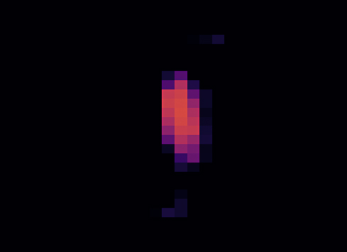
Figure 4: Mean integrated gradient explanation for a binary GP classifier (= single GP + sigmoid activation + Bernoulli likelihood) - brighter sections indicate that the respective sections steer the classifier towards predicting the correct digit.

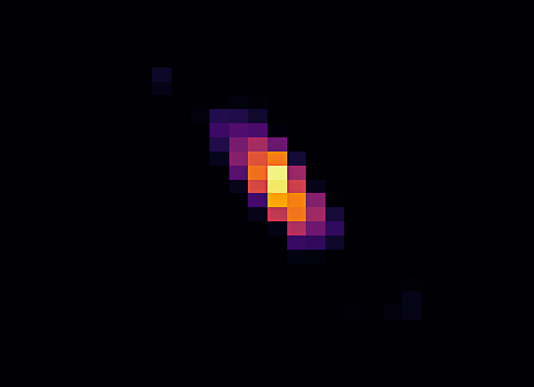
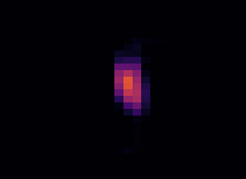
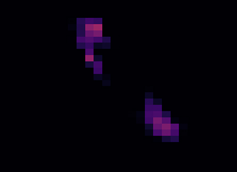
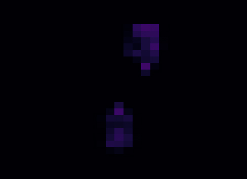
Figure 5: Mean integrated gradient explanation for a 2-class multiclass GP classifier (= 2 GPs + softmax activation + Categorical likelihood) - Top: Brighter sections indicate that the respective sections steer the classifier towards predicting the correct digit as per the example images. Bottom: Brighter sections indicate that the respective sections steer the classifier towards predicting the wrong digit.

7 Discussion

As we have seen, gradient-based explanations for GP models with Gaussian likelihood are easily derived from their standard formulation by merely exchanging the corresponding kernel matrices. In the classification case, it is necessary to resort to approximation or MC-estimation. Using the proposed method, it is possible to reasonably approximate the mean of the posterior explanation. With a restriction on independent GPs, it is also possible to derive a feasible approximation in the multiclass case.

Limitations. As we limited ourselves to independent GPs, corresponding multi-class models might not be able to accurately fit the problem and hence generate sub-optimal predictive performance. Allowing for correlation between the GPs in a multi-class classification problem would make (37) and (39) considerably more complex as the cross-GP components (covariances and off-diagonal elements of the Hessian matrix) in the summations would not cancel out as zeros anymore. Theoretically however, interdependent GPs should be possible to handle as well, albeit with a lot more computational effort involved.

Also, contrary to gradient-based explanations in Neural Networks that can be calculated directly via standard autograd tools, the proposed method requires a more sophisticated and less efficient statistical treatment. In fact, the present method only produces approximate explanations in case the likelihood is not Gaussian. For complex posterior distributions, the Taylor approximation might be insufficient as the negligence of higher order moments could yield more inaccurate results.

Outlook and broader context. In regards to the quality of explanations, solving or mitigating the limitations mentioned above might further improve usability for real-world problems. Beyond better explanations, combining explainable machine learning and the concept of prior knowledge from Bayesian Machine Learning could open new possibilities of regularizing a model’s reasoning process by placing human guided prior distributions over model explanations. This could help to formalize and improve the debugging process of erroneous models or provide a meaningful approach towards tackling the problem of biased Machine Learning.

Appendix A Proofs and derivations

Derivation of the integrated gradient for a GP regression posterior function:

$$\hat{IG}_{k}(x)\sim\mathcal{N}\left(x^{(k)}\frac{1}{G}\sum_{g=1}^{G}\tilde{m}_{G}^{\partial_{k}}\left(x\right),x^{(k)}[1/G]^{T}\tilde{K}_{G}(x)[1/G]x^{(k)}\right)$$

Proof This follows directly from applying standard laws on Gaussian random variables - consider the mean vector and covariance matrix for the posterior process evaluated at $g=1,...,g=G$ and presume for the baseline $\tilde{x}=\mathbf{0}$:

$$\tilde{m}_{G}^{\partial_{k}}(x)=\begin{bmatrix}\tilde{m}^{\partial_{k}}(\frac{1}{G}x)\\ \tilde{m}^{\partial_{k}}(\frac{2}{G}x)\\ \vdots\\ \tilde{m}^{\partial_{k}}(\frac{G}{G}x)\end{bmatrix},\quad\tilde{K}_{G}^{\partial_{k}}(x)=\begin{bmatrix}\tilde{k}^{\partial_{k}}(\frac{1}{G}x,\frac{1}{G}x)&\tilde{k}^{\partial_{k}}(\frac{1}{G}x,\frac{2}{G}x)&\cdots&\tilde{k}^{\partial_{k}}(\frac{1}{G}x,\frac{G}{G}x)\\ \tilde{k}^{\partial_{k}}(\frac{2}{G}x,\frac{1}{G}x)&\ddots&&\tilde{k}^{\partial_{k}}(\frac{2}{G}x,\frac{G}{G}x)\\ \vdots&&\ddots&\vdots\\ \tilde{k}^{\partial_{k}}(\frac{G}{G}x,\frac{1}{G}x)&\tilde{k}^{\partial_{k}}(\frac{G}{G}x,\frac{2}{G}x)&\cdots&\tilde{k}^{\partial_{k}}(\frac{G}{G}x,\frac{G}{G}x)\\ \end{bmatrix}$$

applying (12) to the implied random variable $\tilde{f}_{G}^{\partial_{k}}(x)\sim\mathcal{N}(\tilde{m}_{G}^{\partial_{k}}(x),\tilde{K}_{G}^{\partial_{k}}(x))$ amounts to the operation

$${x^{(k)}}\cdot\begin{bmatrix}\frac{1}{G}&\cdots&\frac{1}{G}\end{bmatrix}^{T}\tilde{f}_{G}^{\partial_{k}}(x)$$

from which we obtain

$${x^{(k)}}\cdot\begin{bmatrix}\frac{1}{G}&\cdots&\frac{1}{G}\end{bmatrix}^{T}\tilde{m}_{G}^{\partial_{k}}(x)=x^{(k)}\frac{1}{G}\sum_{g=1}^{G}\tilde{m}_{G}^{\partial_{k}}\left(x\right)$$

and

$${x^{(k)}}\cdot\begin{bmatrix}\frac{1}{G}&\cdots&\frac{1}{G}\end{bmatrix}^{T}\tilde{K}_{G}^{\partial_{k}}(x)\begin{bmatrix}\frac{1}{G}&\cdots&\frac{1}{G}\end{bmatrix}\cdot{x^{(k)}}=x^{(k)}[1/G]^{T}\tilde{K}_{G}(x)[1/G]x^{(k)}$$

which proves (24).

It can be seen that $\hat{IG}_{k}$ follows a Gaussian Process over all $x\in\mathcal{X}$ and all partial derivatives $k$.

Proof of Proposition 1

We have for the joint distribution of $f_{*}$, $f_{*}^{\partial_{k}}$ and $u_{M}$:

$$p(f_{*},f_{*}^{\partial_{k}},u_{M})=\mathcal{N}\left(\begin{bmatrix}f_{*}\\ f_{*}^{\partial_{k}}\\ u_{M}\end{bmatrix}\Bigg{|}\begin{bmatrix}m_{*}\\ m_{*}^{\partial_{k}}\\ u_{M}\end{bmatrix},\begin{bmatrix}K_{**}&K_{**}^{\partial_{k}^{\prime}}&K_{*M}\\ K_{**}^{\partial_{k}}&K_{**}^{\partial_{k}\partial^{\prime}_{k}}&K_{*M}^{\partial_{k}}\\ K_{M*}&K_{M*}^{\partial_{k}^{\prime}}&K_{MM}\par\end{bmatrix}\right)$$ (40)

Thus, we get

$$\begin{gathered}q(f_{*}^{\partial_{k}})=\int\int p(f_{*},f_{*}^{\partial_{k}}|u_{M})q(u_{M})\,df_{*}du_{M}\\ =\int\int p(f_{*},f_{*}^{\partial_{k}}|u_{M})df_{*}q(u_{M})\,du_{M}\\ =\int p(f_{*}^{\partial_{k}}|u_{M})q(u_{M})\,du_{M}\\ =\int\mathcal{N}(f_{*}^{\partial_{k}}|m_{*}^{\partial_{k}}+K_{*M}^{\partial_{k}}K_{MM}^{-1}(u_{M}-m_{M}),K_{**}-K_{*M}^{\partial_{k}}K_{MM}^{-1}K_{M*}^{\partial_{k}})\mathcal{N}(u_{M}|a,S)\,du_{M}\\ =\mathcal{N}(f_{N}^{\partial_{k}}|m_{*}^{\partial_{k}}+K_{*M}^{\partial_{k}}K_{MM}^{-1}(a-m_{M}),K_{**}-\tilde{\Lambda}_{*M}^{\partial_{k}}(K_{MM}-S)\tilde{\Lambda}_{M*}^{\partial^{\prime}_{k}}){\qed}\end{gathered}$$ (41)

Derivation of the Taylor approximation for $\mathbb{E}\left[\sigma^{\prime}(\tilde{f})\cdot\tilde{f}^{\partial_{k}}\right]$ in (35):

$$\mathbb{E}\left[\sigma^{\prime}(\tilde{f})\cdot\tilde{f}^{\partial_{k}}\right]\approx\sigma^{\prime}(\tilde{m})\cdot\tilde{m}^{\partial_{k}}+\frac{\tilde{s}^{2}}{2}\left\{\sigma^{\prime\prime\prime}(\tilde{m})\left[\tilde{m}^{\partial_{k}}+\frac{\tilde{k}^{\partial_{k}}}{\tilde{k}}\right]+2\frac{\tilde{k}^{\partial_{k}}}{\tilde{k}}\sigma^{\prime\prime}(\tilde{m})\right\}$$

Proof Let $g(\tilde{f})=\left[\sigma^{\prime}(\tilde{f})\cdot\left(\tilde{m}^{\partial}+\frac{\tilde{k}^{\partial}}{\tilde{k}}(\tilde{f}-\tilde{m})\right)\right]$ and write $\mathbb{E}\left[\sigma^{\prime}(\tilde{f})\cdot\tilde{f}^{\partial_{k}}\right]=\mathbb{E}[g(\tilde{f})]$ as a direct consequence of Proposition 2. Clearly, $g(\cdot)\in C^{\infty}$ and $\tilde{f}$, being a Gaussian random variable, has existing moments up to infinite order - hence a standard Taylor approximation is possible:

$$\mathbb{E}[g(\tilde{f})]=\mathbb{E}[g(\tilde{f})]=\mathbb{E}[g(\tilde{m}+(\tilde{f}-\tilde{m}))]$$

$$\approx\mathbb{E}[g(\tilde{m})]+\mathbb{E}[g^{\prime}(\tilde{m})(\tilde{f}-\tilde{m})]+\frac{1}{2}\mathbb{E}[g^{\prime\prime}(\tilde{m})(\tilde{f}-\tilde{m})^{2}]$$

$$=\mathbb{E}[g(\tilde{m})]+g^{\prime}(\tilde{m})\mathbb{E}[\tilde{f}-\tilde{m}]+\frac{1}{2}g^{\prime\prime}(\tilde{m})\mathbb{E}[(\tilde{f}-\tilde{m})^{2}]$$

$$=\mathbb{E}[g(\tilde{m})]+\frac{s^{2}}{2}g^{\prime\prime}(\tilde{m})$$ (42)

Plugging back in the full expression for $g(\cdot)$ and calculating the derivatives:

$$g(\tilde{m})=\sigma^{\prime}(\tilde{m})\cdot\left(\tilde{m}^{\partial}+\frac{\tilde{k}^{\partial}}{\tilde{k}}(\tilde{m}-\tilde{m})\right)=\sigma^{\prime}(\tilde{m})\cdot\tilde{m}^{\partial}$$

$$g^{\prime}(\tilde{m})=\sigma^{\prime\prime}(\tilde{m})\cdot\tilde{m}^{\partial}+\sigma^{\prime\prime}(\tilde{m})\frac{\tilde{k}^{\partial}}{\tilde{k}}\tilde{m}+\sigma^{\prime}(\tilde{m})\frac{\tilde{k}^{\partial}}{\tilde{k}}-\sigma^{\prime\prime}(\tilde{m})\frac{\tilde{k}^{\partial}}{k}\tilde{m}$$

$$=\sigma^{\prime\prime}(\tilde{m})\cdot\tilde{m}^{\partial}+\sigma^{\prime}(\tilde{m})\frac{\tilde{k}^{\partial}}{\tilde{k}}$$

$$\begin{gathered}g^{\prime\prime}(\tilde{m})=\sigma^{\prime\prime\prime}(\tilde{m})\cdot\tilde{m}^{\partial}+\sigma^{\prime\prime\prime}(\tilde{m})\frac{\tilde{k}^{\partial}}{\tilde{k}}\tilde{m}+\sigma^{\prime\prime}(\tilde{m})\frac{\tilde{k}^{\partial}}{\tilde{k}}+\sigma^{\prime\prime}(\tilde{m})\frac{\tilde{k}^{\partial}}{\tilde{k}}-\sigma^{\prime\prime\prime}(\tilde{m})\frac{\tilde{k}^{\partial}}{\tilde{k}}\\ \end{gathered}$$ (43)

Appendix B Experiment details

Implementation

All experiments were performed in Julia (Bezanson et al. [2017]) using Zygote (Innes et al. [2019]) and Flux (Innes et al. [2018]) for autograd.

All SVGPs used 10 inducing points and a SE kernel. For the classification models, the SVGPs were initialized by randomly drawing 10 input examples from the training dataset on initialization.

The models were trained using the Flux.ADAM optimizer with a learning rate of $0.01$ and uniform random batch sampling with $50$ samples per batch.

Boston housing - dataset description

crim - per capita crime rate by town
zn - proportion of residential land zoned for lots over 25,000 sq.ft.
indus - proportion of non-retail business acres per town.
chas - Charles River dummy variable (1 if tract bounds river; 0 otherwise)
nox - nitric oxides concentration (parts per 10 million)
rm - average number of rooms per dwelling
age - proportion of owner-occupied units built prior to 1940
dis - weighted distances to five Boston employment centres
rad - index of accessibility to radial highways
tax - full-value property-tax rate per $10,000
ptratio - pupil-teacher ratio by town
b - $1000(Bk-0.63)^{2}$ where $Bk$ is the proportion of blacks by town
lstat - % lower status of the population
medv - Median value of owner-occupied homes in $1000’s (target variable)

References

- Snelson and Ghahramani [2006] Edward Snelson and Zoubin Ghahramani. Sparse gaussian processes using pseudo-inputs. Advances in neural information processing systems, 18:1257, 2006.
- Van der Wilk et al. [2017] Mark Van der Wilk, Carl Edward Rasmussen, and James Hensman. Convolutional gaussian processes. arXiv preprint arXiv:1709.01894, 2017.
- Tipping [2001] Michael E Tipping. Sparse bayesian learning and the relevance vector machine. Journal of machine learning research, 1(Jun):211–244, 2001.
- Williams and Rasmussen [2006] Christopher K Williams and Carl Edward Rasmussen. Gaussian processes for machine learning, volume 2. MIT press Cambridge, MA, 2006.
- Guyon et al. [2004] Isabelle Guyon, Steve Gunn, Asa Ben-Hur, and Gideon Dror. Result analysis of the nips 2003 feature selection challenge. In L. Saul, Y. Weiss, and L. Bottou, editors, Advances in Neural Information Processing Systems, volume 17. MIT Press, 2004. URL https://proceedings.neurips.cc/paper/2004/file/5e751896e527c862bf67251a474b3819-Paper.pdf.
- Schölkopf et al. [2002] Bernhard Schölkopf, Alexander J Smola, Francis Bach, et al. Learning with kernels: support vector machines, regularization, optimization, and beyond. MIT press, 2002.
- Duvenaud et al. [2011] David K Duvenaud, Hannes Nickisch, and Carl Rasmussen. Additive gaussian processes. Advances in neural information processing systems, 24, 2011.
- Solak et al. [2002] Ercan Solak, Roderick Murray-Smith, WE Leithead, D Leith, and Carl Rasmussen. Derivative observations in gaussian process models of dynamic systems. Advances in neural information processing systems, 15, 2002.
- Eriksson et al. [2018] David Eriksson, Kun Dong, Eric Lee, David Bindel, and Andrew G Wilson. Scaling gaussian process regression with derivatives. Advances in neural information processing systems, 31, 2018.
- De Roos et al. [2021] Filip De Roos, Alexandra Gessner, and Philipp Hennig. High-dimensional gaussian process inference with derivatives. In International Conference on Machine Learning, pages 2535–2545. PMLR, 2021.
- Rasmussen [2003] Carl Edward Rasmussen. Gaussian processes in machine learning. In Summer school on machine learning, pages 63–71. Springer, 2003.
- Titsias [2009] Michalis K. Titsias. Variational learning of inducing variables in sparse gaussian processes. In David A. Van Dyk and Max Welling, editors, Proceedings of the Twelfth International Conference on Artificial Intelligence and Statistics, AISTATS 2009, Clearwater Beach, Florida, USA, April 16-18, 2009, volume 5 of JMLR Proceedings, pages 567–574. JMLR.org, 2009. URL http://proceedings.mlr.press/v5/titsias09a.html.
- Hensman et al. [2013] James Hensman, Nicoló Fusi, and Neil D. Lawrence. Gaussian processes for big data. In Ann Nicholson and Padhraic Smyth, editors, Proceedings of the Twenty-Ninth Conference on Uncertainty in Artificial Intelligence, UAI 2013, Bellevue, WA, USA, August 11-15, 2013. AUAI Press, 2013. URL https://dslpitt.org/uai/displayArticleDetails.jsp?mmnu=1&smnu=2&article_id=2389&proceeding_id=29.
- Hensman et al. [2015a] James Hensman, Alexander G. de G. Matthews, and Zoubin Ghahramani. Scalable variational gaussian process classification. In Guy Lebanon and S. V. N. Vishwanathan, editors, Proceedings of the Eighteenth International Conference on Artificial Intelligence and Statistics, AISTATS 2015, San Diego, California, USA, May 9-12, 2015, volume 38 of JMLR Workshop and Conference Proceedings. JMLR.org, 2015a. URL http://proceedings.mlr.press/v38/hensman15.html.
- Montavon et al. [2018] Grégoire Montavon, Wojciech Samek, and Klaus-Robert Müller. Methods for interpreting and understanding deep neural networks. Digit. Signal Process., 73:1–15, 2018. doi:10.1016/j.dsp.2017.10.011. URL https://doi.org/10.1016/j.dsp.2017.10.011.
- Simonyan et al. [2013] Karen Simonyan, Andrea Vedaldi, and Andrew Zisserman. Deep inside convolutional networks: Visualising image classification models and saliency maps. arXiv preprint arXiv:1312.6034, 2013.
- Sundararajan et al. [2017] Mukund Sundararajan, Ankur Taly, and Qiqi Yan. Axiomatic attribution for deep networks. In International Conference on Machine Learning, pages 3319–3328. PMLR, 2017.
- Hendriks et al. [2018] Johannes N Hendriks, Carl Jidling, Adrian Wills, and Thomas B Schön. Evaluating the squared-exponential covariance function in gaussian processes with integral observations. arXiv preprint arXiv:1812.07319, 2018.
- Hensman et al. [2015b] James Hensman, Alexander Matthews, and Zoubin Ghahramani. Scalable variational gaussian process classification. In Artificial Intelligence and Statistics, pages 351–360. PMLR, 2015b.
- Kingma and Welling [2013] Diederik P Kingma and Max Welling. Auto-encoding variational bayes. arXiv preprint arXiv:1312.6114, 2013.
- Minai and Williams [1993] Ali A Minai and Ronald D Williams. On the derivatives of the sigmoid. Neural Networks, 6(6):845–853, 1993.
- Jankowiak et al. [2020] Martin Jankowiak, Geoff Pleiss, and Jacob Gardner. Parametric gaussian process regressors. In International Conference on Machine Learning, pages 4702–4712. PMLR, 2020.
- Bezanson et al. [2017] Jeff Bezanson, Alan Edelman, Stefan Karpinski, and Viral B Shah. Julia: A fresh approach to numerical computing. SIAM review, 59(1):65–98, 2017. URL https://doi.org/10.1137/141000671.
- Innes et al. [2019] Mike Innes, Alan Edelman, Keno Fischer, Christopher Rackauckas, Elliot Saba, Viral B. Shah, and Will Tebbutt. A differentiable programming system to bridge machine learning and scientific computing. CoRR, abs/1907.07587, 2019. URL http://arxiv.org/abs/1907.07587.
- Innes et al. [2018] Michael Innes, Elliot Saba, Keno Fischer, Dhairya Gandhi, Marco Concetto Rudilosso, Neethu Mariya Joy, Tejan Karmali, Avik Pal, and Viral Shah. Fashionable modelling with flux. CoRR, abs/1811.01457, 2018. URL https://arxiv.org/abs/1811.01457.